H3DTDinv – MUMPS

A Program Library for Forward Modelling of Multi-Transmitter, Time-Domain Electromagnetic Data over 3D structures.

Version 1.0

Developed under the MITEM consortium Research Project Multi-Source Inversion of Time Domain Electromagnetic Data

UBC Geophysical Inversion Facility

Department of Earth and Ocean Sciences University of British Columbia Vancouver, British Columbia

http://www.eos.ubc.ca/research/ubcgif/

© UBC Geophysical Inversion Facility, September 2010

Introduction

H3DTDinv is a flexible program library for inversion of geophysical time domain electromagnetic

survey data resulting from a wide range of sources and source waveforms. The objective of

H3DTDinv is to recover a 3D model of the earth’s electrical conductivity structure, discretized

using a mesh of rectangular cells. This recovery of geo-electrical parameters is achieved

through an iterative process, which includes 3D forward simulation at each step and

minimization of the objective function (, which, in turn is controlled by data misfit (d) and the

model norm (m). The forward simulation is solving Maxwell’s equations in the time domain. The

equations are discretized in time using backward Euler method and discretized in space by

using a finite volume technique on a staggered grid. The sources can be grounded dipoles or

loop currents that reside in the air, on the surface, or inside the earth. The responses can be

any combination of components of E, H, or dB/dt. The transmitter waveform is user-defined and

there are no restrictions on the length or shape of the waveform. The Earth model is an arbitrary

3D conductivity distribution, defined on a structured rectangular mesh.

From the user's viewpoint, the software operates much like EH3DTDinv, a previous GIF code

developed to carry out time domain inversion. The principal difference is that H3DTDinv

inherently works with many transmitters. To facilitate this multi-transmitter capability, the forward

modelling matrix is first decomposed using Cholesky decomposition, such that the solution for

different transmitters is easily carried out. The solutions are achieved by factorizing the forward

modelling matrix. H3DTDinv, although it requires significant computing resources, under certain

conditions can be run on single modern laptop or desktop computer. Factorization of the forward

modelling matrix is facilitated via the MUMPS software for which documentation and downloads

can be found at the following website: http://graal.ens-lyon.fr/MUMPS/ . Unlike the

forward modelling code, H3DTD, where only one factorization is stored at one time, in

H3DTDinv, all factorizations must be stored at the same time, which requires a lot more RAM.

The MUMPS routines are built-in to H3DTDinv and do not need to be installed separately.

However, since the forward modelling matrix is large and its decomposition is computationally

intensive, H3DTDinv is most efficiently run on an array of computers, or on a single multi-core

computer with lots of RAM (~ 16GB). The parallel implementation is carried out using the

Message Passing Interface standard (MPI), discussed further in this document.

List of the input files and Graphical User Interface utilities (GUI’s)

Programs and GUI’s Input files File names

H3DTDinv.exe Input control file h3dtdinv.inp (fixed name)

Conductivity model files (initial, reference)

model_ini.txt (user defined)

model_ref.txt ( user defined)

Data file data.dat (user-defined)

Topography file topo.dat (user-defined)

Weighting file weight.txt (user-defined)

Mesh_builder.exe GUI Mesh file mesh.txt ( user defined )

Wave_builder.exe GUI Wave file wave.txt ( user defined )

Table 1. List of H3DTDinv components and control files (green color indicates that these files are not mandatory to run the inversion).

Setting up the control files

“H3DTDinv.exe” is the executable for the 3D time domain inversion. It has to be run in a

separate folder (further “workdir”), which also contains the input file “h3dtdinv.inp”. The

remainder of the input files do not have any strict naming convention and can be located in any

hard drive or network location under any name, as long as they are properly referenced in the

“h3dtdinv.inp” file. However for convenience we recommend keeping all files relevant to a single

inversion in your “workdir”.

H3DTDinv requires a number of input files and parameters. The control file “h3dtdinv.inp”

contains references to all necessary files in the 15-line format (see an example below):

mesh.txt ! mesh file

VALUE 0.01 | FILE model_ini.con ! initial conductivity file

VALUE 0.01 | FILE model_ref.con ! reference conductivity file

data_H.txt ! data file

wave.txt ! wave file

TOPO_CONST 0. | TOPO_FILE topo.dat

ignore

BOUNDS_NONE ! BOUNDS_NONE | BOUNDS_CONST bl bu | BOUNDS_FILE file

NONE ! weight file

1.e+2 1.e-9 0.2 ! beta_max beta_min beta_factor

1.e-4 1. 1. 1. ! alpha

CHANGE_MREF ! CHANGE_MREF | NOT_CHANGE_MREF

SMOOTH_MOD_DIF ! SMOOTH_MOD | SMOOTH_MOD_DIF

1. ! chifact

3 10 1.e-3 ! max_iter_beta max_iter_ipcg tol_ipcg

In this example there are several other supplementary input files listed, which are described

below:

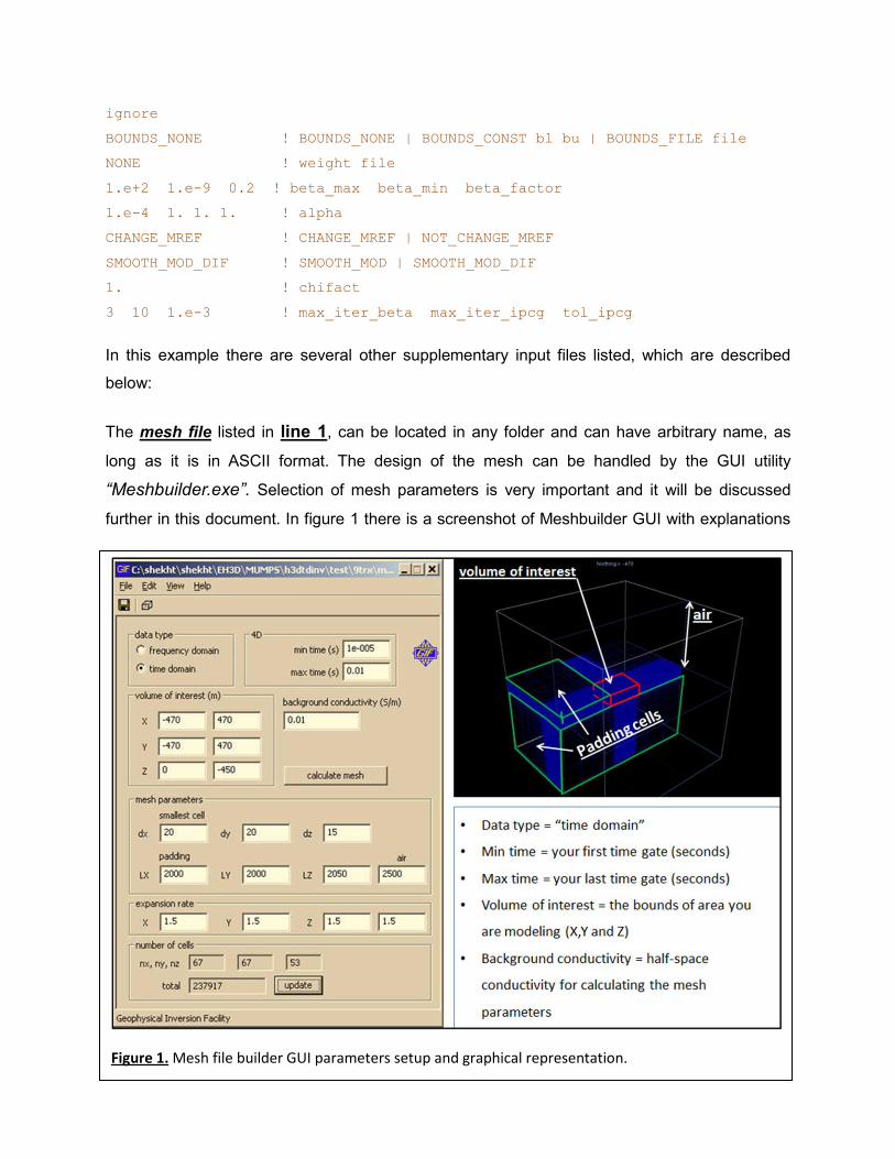
The mesh file listed in line 1, can be located in any folder and can have arbitrary name, as

long as it is in ASCII format. The design of the mesh can be handled by the GUI utility

“Meshbuilder.exe”. Selection of mesh parameters is very important and it will be discussed

further in this document. In figure 1 there is a screenshot of Meshbuilder GUI with explanations

Figure 1. Mesh file builder GUI parameters setup and graphical representation.

of described parameters”. In setting the mesh parameters, the cell size of “volume of interest”

(“smallest cell” in the menu) should depend on the actual geometry of the survey (primarily on

density of stations defined by line spacing and sampling rate). The user has to maintain a

balance between saving computing time (by coarsening the mesh) and getting more accurate

solution of the forward simulation by making the mesh finer. The padding distance, depends on

the latest data acquisition time gate and is calculated automatically to diffusion distance defined

by equation (1):

(1) D(t) = 1250*√𝒕𝝈⁄ (meters)

In this equation t is the latest time gate and is the conductivity of the background half-space

in Siemens per meter (S/m).

The background conductivity in meshbuilder is only used to calculate the diffusion radius and is

not being further assigned for the forward starting model. The expansion rate is the geometric

progression coefficient used for building the padding cells. Generally values between 1.3 and

1.6 are reasonable choices for the expansion rate.

The format of the mesh file is:

nx ny nz (number of cells in the X, Y, and Z directions)

x0 y0 z0 (coordinates of the top south west corner of the mesh)

dx_1 dx_2 ... dx_nx (cell widths in X)

dy_1 dy_2 ... dy_ny (cell widths in Y)

dz_1 dz_2 ... dz_nz (cell widths in Z)

The initial model file is the starting model for the initial forward simulation. It is referenced in

line 2 of the input control file, and is defined in the standard UBC format, as a single column of

values, one value for each cell. The first value corresponds to the top south-western cell. The

values are ordered such that Z (depth) changes the fastest, followed by X (easting), followed by

Y (northing). For constant half-space model parameters, a single value entered in the input

control file can be used as a substitute to the model files. When a file is entered, the line in the

input file should start with “FILE”, and when a constant value is entered, the line should start

with VALUE. The model is updated after every iterative step and used to calculate data misfit.

Each updated model is written in the workdir with a new name “inv_*.con”, containing the

iteration number.

The reference model file is specified in line 3 of the input control file. It may or may not be

updated throughout the inversion process, depending on a user-defined optional parameter.

The file has identical format to that of the initial model and can be also produced using the

“Modelbuilder v1.0” package. This file is used to calculate the model norm (m). The reference

model may as well be the same as the starting model if no specific geological constraints are

known.

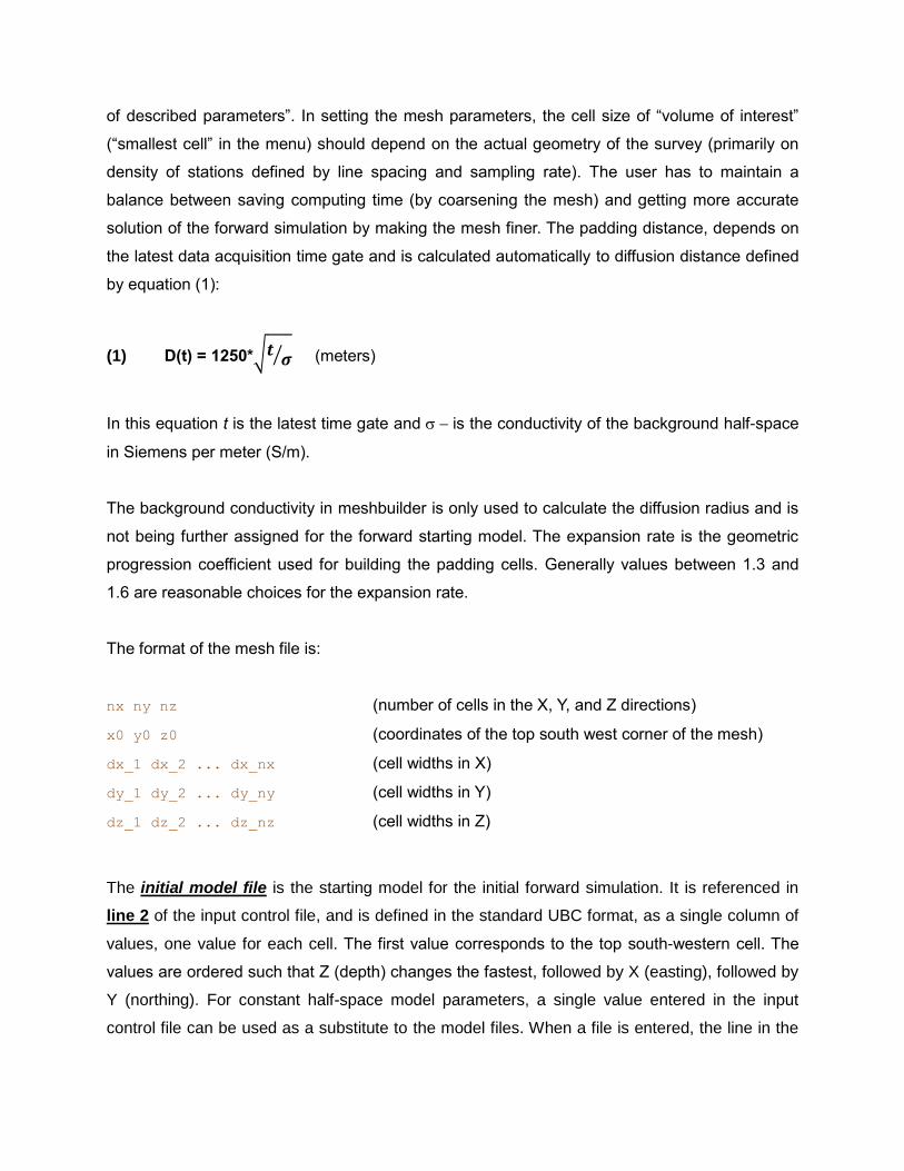
The data file is specified in line 4 of the input control file. This file contains information about

transmitter and receiver locations, acquisition time windows, the measured data and the

standard deviations. In figure 2 the format of the data file is shown.

The format of this file allows complete freedom of using any combination of electric and/or

magnetic field components or magnetic induction derivative components (dB/dt) defined in

Cartesian metric coordinate system (XYZ) and specified in SI units. Each data value must be

followed by its standard deviation. Unfortunately there is no actual time domain system, which

is able to acquire all of these data and most common time domain data comes in units of

magnetic induction time derivative (dB/dt). Therefore a character string is included (Figure 2),

Figure 2. Format of data.dat file for H3DTDinv program.

which would specify the dummy values to be ignored in the data file. For example if only dBz/dt

measurements are provided in a particular data set then all other E, H and dBx/dt or dBy/dt

components in the file should be set to this “dummy” value.

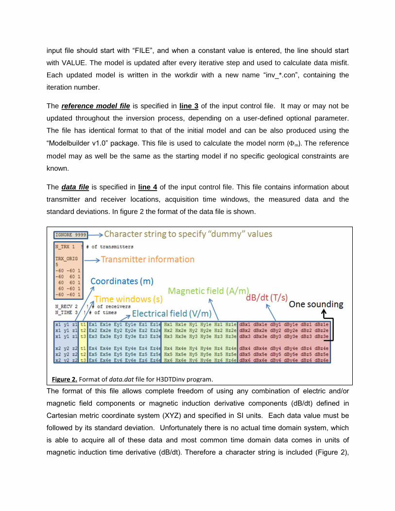
One of the most important features of the H3DTDinv is the ability to invert data from multiple

transmitters. This feature makes it possible to invert airborne time domain data in 3D, as well as

multiple source ground EM soundings. The number of transmitters is specified in the second

line of data file (N_TRX). The transmitter label (i.e., “TRX_ORIG”) is specified in the third line of

the file and indicates the type of transmitter. There are four options for describing the transmitter

source (Figure 3):

TRX_ORIG (Figure 3A,B): connecting individual wire segments to form a grounded or

inductive source

TRX_LINES (Figure 3A): primary field is generated from analytic expressions for wires in

free space

TRX_LOOP (Figure 3C): circular loop with arbitrary orientation

TRX_MAGNETIC_DIPOLE (Figure 3D): magnetic dipole

TRX_ORIG : the “original” distributed current source (closed loops or grounded wires). This type

is a good approximation of any conventional large square loop system (ground and airborne),

including, Crone, Geonics (EM47, 57, 67), Zonge, GeoTEM, MegaTEM, MegaTEM II, SkyTEM,

Figure 3. (A) Original or TRX_LINES transmitter type configuration using closed loop source geometry;

(B) Original transmitter configuration based on grounded wire source geometry (C) Loop transmitter

type (D) Magnetic dipole transmitter type.

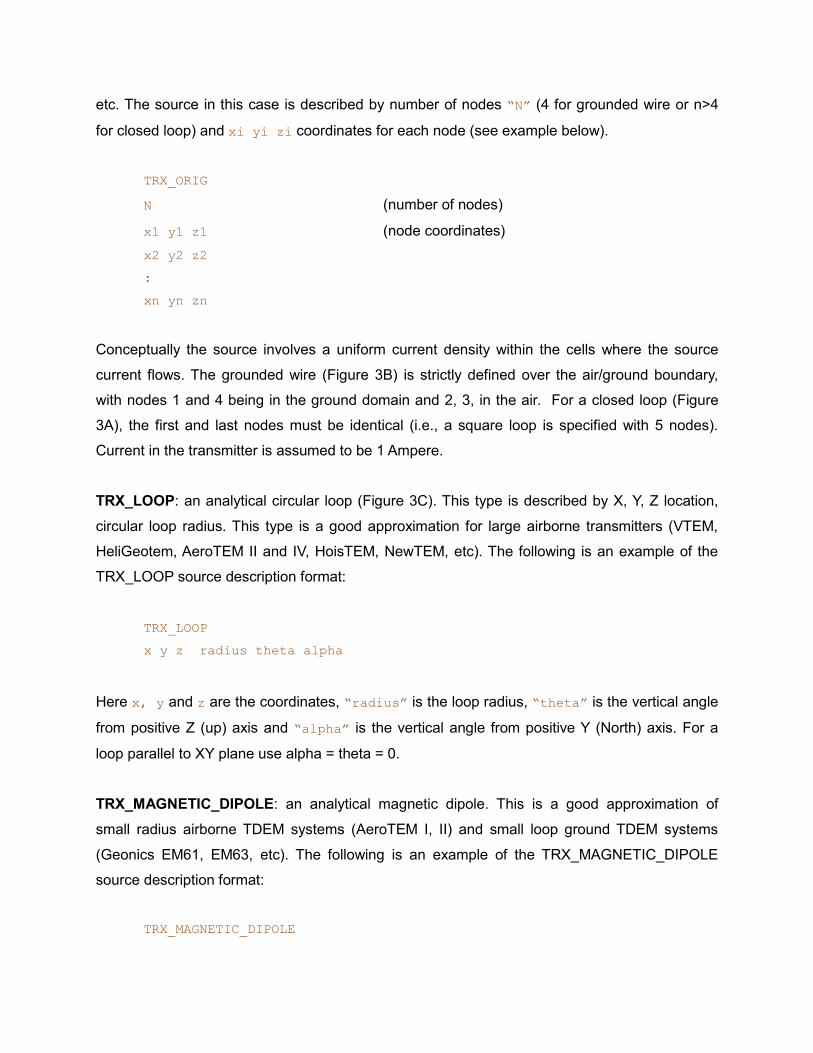
etc. The source in this case is described by number of nodes “N” (4 for grounded wire or n>4

for closed loop) and xi yi zi coordinates for each node (see example below).

TRX_ORIG

N (number of nodes)

x1 y1 z1 (node coordinates)

x2 y2 z2

:

xn yn zn

Conceptually the source involves a uniform current density within the cells where the source

current flows. The grounded wire (Figure 3B) is strictly defined over the air/ground boundary,

with nodes 1 and 4 being in the ground domain and 2, 3, in the air. For a closed loop (Figure

3A), the first and last nodes must be identical (i.e., a square loop is specified with 5 nodes).

Current in the transmitter is assumed to be 1 Ampere.

TRX_LOOP: an analytical circular loop (Figure 3C). This type is described by X, Y, Z location,

circular loop radius. This type is a good approximation for large airborne transmitters (VTEM,

HeliGeotem, AeroTEM II and IV, HoisTEM, NewTEM, etc). The following is an example of the

TRX_LOOP source description format:

TRX_LOOP

x y z radius theta alpha

Here x, y and z are the coordinates, “radius” is the loop radius, “theta” is the vertical angle

from positive Z (up) axis and “alpha” is the vertical angle from positive Y (North) axis. For a

loop parallel to XY plane use alpha = theta = 0.

TRX_MAGNETIC_DIPOLE: an analytical magnetic dipole. This is a good approximation of

small radius airborne TDEM systems (AeroTEM I, II) and small loop ground TDEM systems

(Geonics EM61, EM63, etc). The following is an example of the TRX_MAGNETIC_DIPOLE

source description format:

TRX_MAGNETIC_DIPOLE

x y z theta alpha m

In this file format, x, y and z are the coordinates, “theta” is the vertical angle from positive Z

(up) axis, “alpha” is the vertical angle from positive Y (North) axis and “m” is the dipole

moment of the transmitter, which should be listed in SI units. Similar to previous example, for a

loop parallel to XY plane use alpha = theta = 0.

TRX_LINES: an analytical general closed loop of line currents. It is designed to handle arbitrary

complex transmitters with user defined number of nodes. The format for this source type is

same as for the TRX_ORIG. The number of nodes has to be greater than 4. The main

difference is in numerical algorithms, simulating transmitter currents.

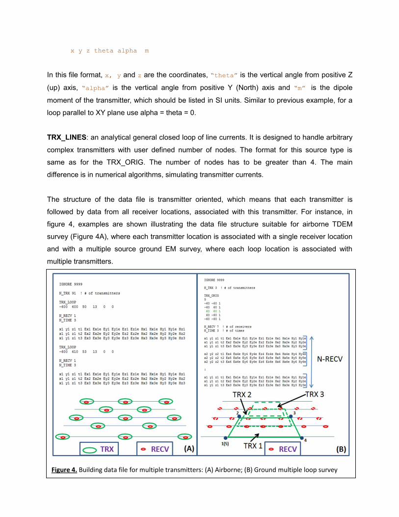
The structure of the data file is transmitter oriented, which means that each transmitter is

followed by data from all receiver locations, associated with this transmitter. For instance, in

figure 4, examples are shown illustrating the data file structure suitable for airborne TDEM

survey (Figure 4A), where each transmitter location is associated with a single receiver location

and with a multiple source ground EM survey, where each loop location is associated with

multiple transmitters.

Figure 4. Building data file for multiple transmitters: (A) Airborne; (B) Ground multiple loop survey

The wave file is specified in line 5 of the input control file. Its format is similar to previous UBC-

GIF codes (EH3DTD). The same wave file is used for all transmitters. Users will likely have their

own wave file for their transmitter. The wave file has control over the discretization of the actual

waveform in both on-time and off-time. This discretization is carried out by defining time

stepping “t”, used to solve Maxwell’s equations in time domain. This time stepping is used for

factorization of the modeling matrix. A new factorization of the modelling matrix is required

whenever the stepping time “t” is changed. Maxwell's equations are most efficiently solved for

a constant time step or a few time intervals each with a constant time step. Since the inversion

needs to store all factorizations in memory, having many different “t” would require a lot of

RAM.

The most computationally efficient discretization is when a single value of t can be used for the

full time range of interest. Most systems consist of an “on-time” portion (exponential, half-sign,

ramp, etc) followed by an “off-time”. The on-time portion of the waveform may be modelled

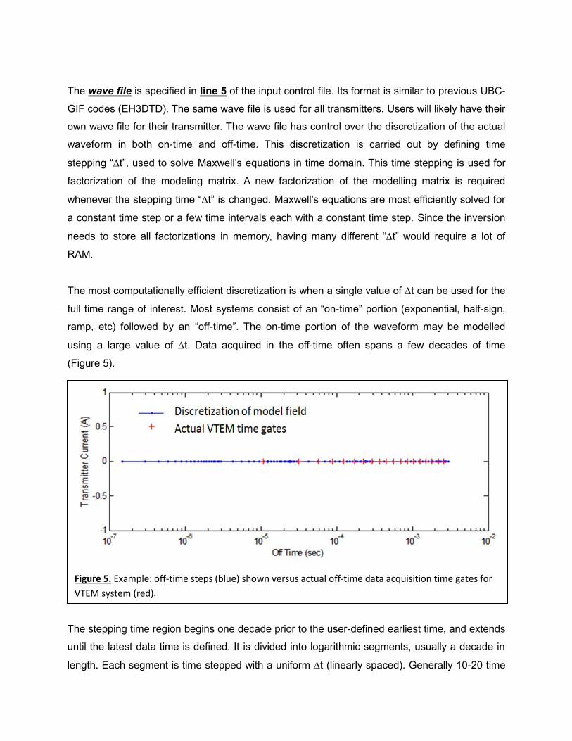
using a large value of t. Data acquired in the off-time often spans a few decades of time

(Figure 5).

The stepping time region begins one decade prior to the user-defined earliest time, and extends

until the latest data time is defined. It is divided into logarithmic segments, usually a decade in

length. Each segment is time stepped with a uniform t (linearly spaced). Generally 10-20 time

Figure 5. Example: off-time steps (blue) shown versus actual off-time data acquisition time gates for

VTEM system (red).

steps are adequate for each decade in time. The total computation time depends upon the

number of factorizations, the number of time steps, and the number of transmitters. Please note,

that if time stepping does not match the actual data acquisition time windows, interpolated

values of the fields are assigned to the predicted data at times specified in the data file.

A “Wavebuilde.exe” GUI has been provided with the inversion code to assist the user in

generating the wave files. Figures 6, 7 and 8 show the user interface for generating different

types of waveforms. Among the GUI settings there are some general parameters, which are

applicable to any waveform and other parameters specific to each waveform type in particular.

Among the general parameters are the following:

Max/min: “min” and “max” values denote the beginning and end values of the time

window through which equations are time-stepped. “min” should be smaller (typically about a

decade) smaller than the first datum time. “max” can correspond to the last datum time.

# of segments and # of samples per segment are the number of logarithmically spaced

segments and linearly spaced samples per each segment

There are three wave type options included in the present GUI.

Step off (Figure 6)

UTEM (Figure 7)

Exponential plus a ramp (Figure 8)

Each of these are described in further detail below, accompanied by explanations of the

parameters of the interface that are of relevance, and also plots of the times at which the

equations are solved. For each waveform type all time values are referenced to the “time zero”,

which is the beginning of both: factorization time steps and data acquisition time gates.

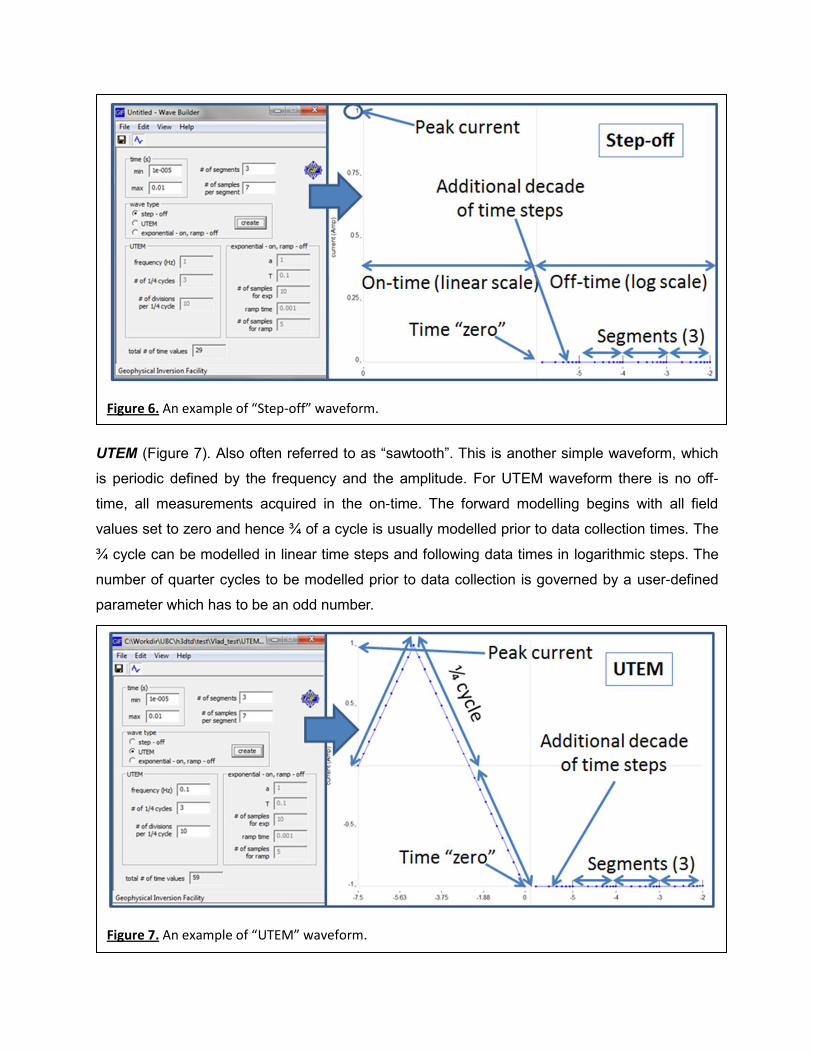
Step-off (Figure 6). The current prior to t=0 is assumed to be uniform and solution of the steady

state fields are generated by the program. This reverse Heaviside function is the simplest

waveform to model. No actual geophysical system uses this exact waveform; however recorded

signals can often be deconvolved to conform to this waveform type. Peak current (maximum

current) data are generally sampled only in the log domain.

UTEM (Figure 7). Also often referred to as “sawtooth”. This is another simple waveform, which

is periodic defined by the frequency and the amplitude. For UTEM waveform there is no off-

time, all measurements acquired in the on-time. The forward modelling begins with all field

values set to zero and hence ¾ of a cycle is usually modelled prior to data collection times. The

¾ cycle can be modelled in linear time steps and following data times in logarithmic steps. The

number of quarter cycles to be modelled prior to data collection is governed by a user-defined

parameter which has to be an odd number.

Figure 6. An example of “Step-off” waveform.

Figure 7. An example of “UTEM” waveform.

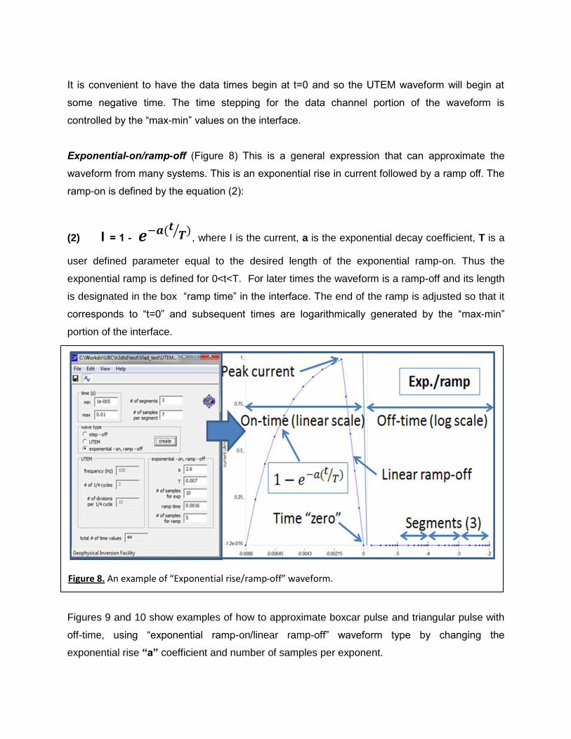
It is convenient to have the data times begin at t=0 and so the UTEM waveform will begin at

some negative time. The time stepping for the data channel portion of the waveform is

controlled by the “max-min” values on the interface.

Exponential-on/ramp-off (Figure 8) This is a general expression that can approximate the

waveform from many systems. This is an exponential rise in current followed by a ramp off. The

ramp-on is defined by the equation (2):

(2) I = 1 - 𝒆−𝒂(𝒕𝑻⁄ )

, where I is the current, a is the exponential decay coefficient, T is a

user defined parameter equal to the desired length of the exponential ramp-on. Thus the

exponential ramp is defined for 0<t<T. For later times the waveform is a ramp-off and its length

is designated in the box “ramp time” in the interface. The end of the ramp is adjusted so that it

corresponds to “t=0” and subsequent times are logarithmically generated by the “max-min”

portion of the interface.

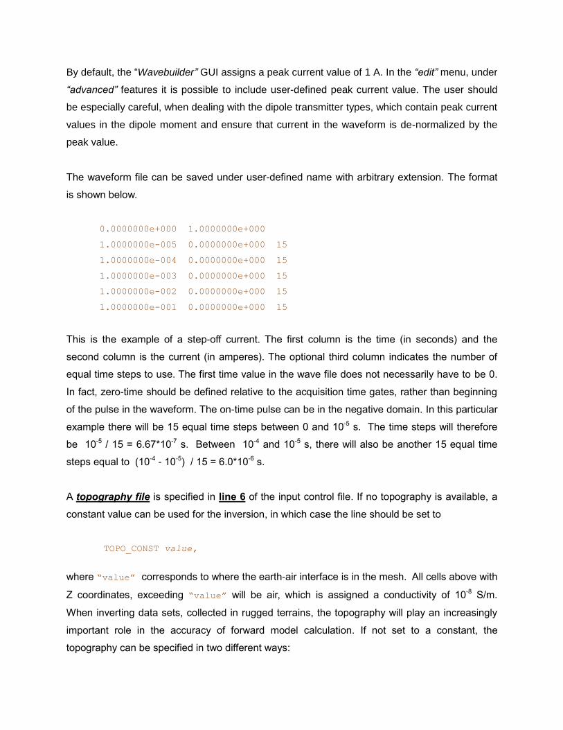
Figures 9 and 10 show examples of how to approximate boxcar pulse and triangular pulse with

off-time, using “exponential ramp-on/linear ramp-off” waveform type by changing the

exponential rise “a” coefficient and number of samples per exponent.

Figure 8. An example of “Exponential rise/ramp-off” waveform.

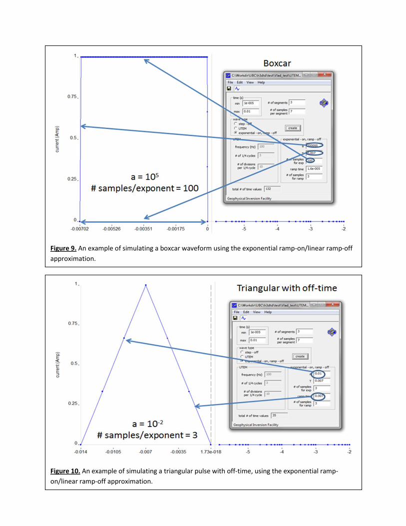
Figure 9. An example of simulating a boxcar waveform using the exponential ramp-on/linear ramp-off

approximation.

Figure 10. An example of simulating a triangular pulse with off-time, using the exponential ramp-

on/linear ramp-off approximation.

By default, the “Wavebuilder” GUI assigns a peak current value of 1 A. In the “edit” menu, under

“advanced” features it is possible to include user-defined peak current value. The user should

be especially careful, when dealing with the dipole transmitter types, which contain peak current

values in the dipole moment and ensure that current in the waveform is de-normalized by the

peak value.

The waveform file can be saved under user-defined name with arbitrary extension. The format

is shown below.

0.0000000e+000 1.0000000e+000

1.0000000e-005 0.0000000e+000 15

1.0000000e-004 0.0000000e+000 15

1.0000000e-003 0.0000000e+000 15

1.0000000e-002 0.0000000e+000 15

1.0000000e-001 0.0000000e+000 15

This is the example of a step-off current. The first column is the time (in seconds) and the

second column is the current (in amperes). The optional third column indicates the number of

equal time steps to use. The first time value in the wave file does not necessarily have to be 0.

In fact, zero-time should be defined relative to the acquisition time gates, rather than beginning

of the pulse in the waveform. The on-time pulse can be in the negative domain. In this particular

example there will be 15 equal time steps between 0 and 10-5 s. The time steps will therefore

be 10-5 / 15 = 6.67*10-7 s. Between 10-4 and 10-5 s, there will also be another 15 equal time

steps equal to (10-4 - 10-5) / 15 = 6.0*10-6 s.

A topography file is specified in line 6 of the input control file. If no topography is available, a

constant value can be used for the inversion, in which case the line should be set to

TOPO_CONST value,

where “value” corresponds to where the earth-air interface is in the mesh. All cells above with

Z coordinates, exceeding “value” will be air, which is assigned a conductivity of 10-8 S/m.

When inverting data sets, collected in rugged terrains, the topography will play an increasingly

important role in the accuracy of forward model calculation. If not set to a constant, the

topography can be specified in two different ways:

1. UBC-GIF standard 3 column topographic file format, specified in line 6 of the

H3DTDinv.inp as: TOPO_FILE topo.dat

n

x1 y1 elev1

x2 y2 elev2

:

xn yn elevn

If topo file is used, all model conductivity values with Z>Ztopo are fixed at 10-8 S/m

2. Using cell masking on a model file. In order to activate this capability, a parameter

MNZ mask_file.dat should be specified in line 6 of the H3DTDinv.inp. of the

“mask_file.dat” file is stored in identical format as the model file and it should contain

values of either 1 or 0, with “1” meaning that this cell will be used for the inversion

(actrive) and “0” meaning that this value is fixed to the corresponding value of the

reference model (inactive).

This masking capability can be potentially used for assigning topography by setting the

reference model cells, corresponding to zeroes in the mask_file.dat to 10-8 S/m.

Line 7 is currently obsolete and is not used by the inversion.

A bounds file may be specified in line 8 of H3DTDinv.inp, with a particular conductivity model.

The bounds are used to put constraints on the inversion. There are three options to set up the

conductivity bounds

BOUNDS_NONE (No bounds are imposed on the conductivity values)

BOUNDS_CONST bl bu (Same bounds for all cells: bl – lower bound, bu – upper bound)

BOUNDS_FILE (A bounds file to be used)

The bounds file has the same number of lines as the model file. It consists of 2 columns,

containing the lower bounds in the first column and the upper bounds in the second column.

Weighting coefficients file is specified in line 9 of the “H3DTDinv.inp” file. User-defined

weights, which are applied to the model norm, are in the same format the model file. A single

column is composed of values greater or equal to one. Each cell’s weight is equal to “1” by

default. It is not recommended to use numbers smaller than “1” as the latter may destabilize the

inversion. By increasing the weighting coefficient of a particular cell, the user is suppressing the

recovery of electrical conductivity for this cell. Weights of inactive cells are ignored.

file.txt is entered for referencing a weighting coefficient file

If NONE is entered, no weighting will be used.

The trade-off parameter is the coefficient used to scale the model norm. The inversion

convergence and stability are in many ways dependant on the correct selection of this

parameter. In line 10 of the control file, the range of trade-off parameter is specified along with

the step used at each iteration. In the inversion we use a cooling algorithm, in accordance with

equation (3), in order to achieve the target misfit.

(3) k+1 = factor*k , where factor is the cooling parameter and i are the

values of trade-off parameter at consequent iteration steps. The range of trade-off parameters

may be entered into H3DTDinv.inp as following:

beta_max beta_min beta_factor, or else set to DEFAULT

During the inversion the trafe-off parameter will start at beta_max and at each iteration it will be

reduced by the factor beta_factor until it reaches beta_min. In case DEFAULT is entered the

trade-off parameter range will be calculated as follows:

Here, r is a random vector, J is the sensitivity matrix and W is the model weighting matrix.

The smoothing parameters may be entered into line 11 of the input control file. These are

𝛽𝑚𝑎𝑥 = 1000∥ 𝐽𝑟 ∥2

∥ 𝑊𝑟 ∥2; 𝛽𝑚𝑖𝑛 = 10−7𝛽𝑚𝑎𝑥; 𝛽𝑓𝑎𝑐𝑡𝑜𝑟 = 0.16681

model objective function parameters used in an identical manner to other UBC-GIF codes. They

should be entered as follows:

alpha_s alpha_x alpha_y alpha_z

Here alpha_s is the coefficient for the smallest model component.

alpha_x is the coefficient for the derivative in the easting direction.

alpha_y is the coefficient for the derivative in the northing direction.

alpha_z is the coefficient for the derivative in the vertical direction.

None of the alpha’s can be negative and they cannot be all equal to 0 at the same time. There

are no default values, the smoothing parameters must be user-defined. They are chosen in an

identical manner to other UBC-GIF codes. Here are some tips:

Consider the ratios: 𝛼𝑥

𝛼𝑠 and

𝛼𝑧

𝛼𝑠. Larger ratios result in smoother models. As a rule of thumb,

keep the following relationships in mind:

𝜶𝒙

𝜶𝒔,

𝜶𝒛

𝜶𝒔≫ 𝟏 The "smoothness" terms dominate in the equation being minimized and the

structure is penalized. Models tend to be as “smooth” as possible. The reference model is less

important.

𝜶𝒙

𝜶𝒔,

𝜶𝒛

𝜶𝒔⇒ 𝟎 The "close to the reference" term dominates in the equation being minimized, so

models may be "rough". The process tries to make a model that looks like the reference, with

smoothness being less important.

To estimate values for the α's for a specific case, start by defining two length scale terms as

follows:

𝑳𝒛 = √𝜶𝒛

𝜶𝒔 and 𝑳𝒙 = √

𝜶𝒙

𝜶𝒔

Then consider these rules of thumb to help choose the α's:

- In general, keep Lx approximately the same as the smallest diffusion radius for the latest time

window and Keep Lx approximately equal to Lz. Also, the following relations are useful:

Lx > mesh cell width

Lz > mesh cell thickness

Lx < total width of the mesh

Lz < total depth of the mesh

Line 12

CHANGE_MREF the reference model will be changed to the recovered model after each beta

iteration.

NOT_CHANGE_MREF the reference model will never be changed.

Line 13

SMOOTH_MOD model norm does not contain the reference model.

SMOOTH_MOD_DIF model norm contains the reference model.

Chifact is specified in Line 14

Target misfit is reached when: data misfit <= chifact * N, where “N” is the total number of data.

This value should usually be equal to 1.

Line 15

max_iter_beta is the user-defined number of iterations to perform for each trade-off

parameter. A good value is about 3 (see “Inversion flowchart” for details).

max_iter_ipcg is the maximum number of IPCG iterations to perform. A good value is

between 10 and 15 (See “inversion flowchart” for details).

tol_ipcg is the stopping tolerance for IPCG iterations. This value should be about 10-3 (see

“inversion flowchart” for details).

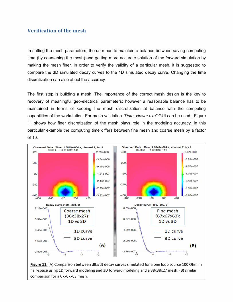
Verification of the mesh

In setting the mesh parameters, the user has to maintain a balance between saving computing

time (by coarsening the mesh) and getting more accurate solution of the forward simulation by

making the mesh finer. In order to verify the validity of a particular mesh, it is suggested to

compare the 3D simulated decay curves to the 1D simulated decay curve. Changing the time

discretization can also affect the accuracy.

The first step is building a mesh. The importance of the correct mesh design is the key to

recovery of meaningful geo-electrical parameters; however a reasonable balance has to be

maintained in terms of keeping the mesh discretization at balance with the computing

capabilities of the workstation. For mesh validation “Data_viewer.exe” GUI can be used. Figure

11 shows how finer discretization of the mesh plays role in the modeling accuracy. In this

particular example the computing time differs between fine mesh and coarse mesh by a factor

of 10.

Figure 11. (A) Comparison between dBz/dt decay curves simulated for a one loop source 100 Ohm m

half-space using 1D forward modeling and 3D forward modeling and a 38x38x27 mesh; (B) similar

comparison for a 67x67x63 mesh.

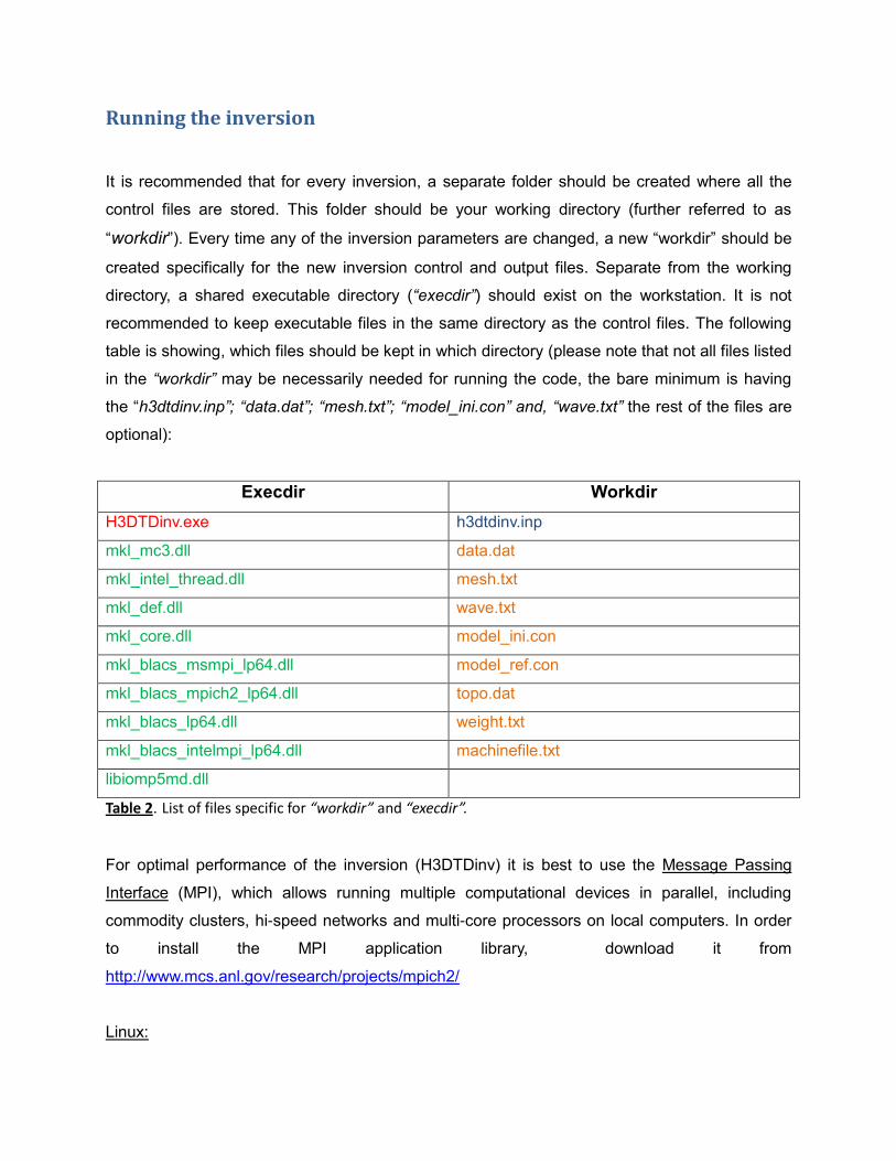
Running the inversion It is recommended that for every inversion, a separate folder should be created where all the

control files are stored. This folder should be your working directory (further referred to as

“workdir”). Every time any of the inversion parameters are changed, a new “workdir” should be

created specifically for the new inversion control and output files. Separate from the working

directory, a shared executable directory (“execdir”) should exist on the workstation. It is not

recommended to keep executable files in the same directory as the control files. The following

table is showing, which files should be kept in which directory (please note that not all files listed

in the “workdir” may be necessarily needed for running the code, the bare minimum is having

the “h3dtdinv.inp”; “data.dat”; “mesh.txt”; “model_ini.con” and, “wave.txt” the rest of the files are

optional):

Execdir Workdir

H3DTDinv.exe h3dtdinv.inp

mkl_mc3.dll data.dat

mkl_intel_thread.dll mesh.txt

mkl_def.dll wave.txt

mkl_core.dll model_ini.con

mkl_blacs_msmpi_lp64.dll model_ref.con

mkl_blacs_mpich2_lp64.dll topo.dat

mkl_blacs_lp64.dll weight.txt

mkl_blacs_intelmpi_lp64.dll machinefile.txt

libiomp5md.dll

Table 2. List of files specific for “workdir” and “execdir”.

For optimal performance of the inversion (H3DTDinv) it is best to use the Message Passing

Interface (MPI), which allows running multiple computational devices in parallel, including

commodity clusters, hi-speed networks and multi-core processors on local computers. In order

to install the MPI application library, download it from

http://www.mcs.anl.gov/research/projects/mpich2/

Linux:

For commodity clusters operated under Linux system, the code can be run on any number of

processors listed in a description ASCII file. The following is an example of such description file:

Compname01:nProc

Compname02:nProc

Compname03:nProc

The description file name is completely arbitrary. “Compname” is the network name of the

computer to be used and “nProc” is the number of processors to be employed for the

procedure. If the computer is on the local network and can be directly accessed, then no path is

needed to be specified. The following is an example of a command line to be used under Linux

operating system in order to start the forward simulation:

mpiexec -machinefile machines.txt -n 20 ./h3dtdinv_mumps

In this command line “-machinefile” calls for a description file “machines.txt” and “–n 20”

indicates a total amount of processors to be used on all the machines listed in the description

file.

Windows:

For single multi-core computer usage, under Windows operating system, the command line will

look like this:

"C:\Program Files\MPICH2\bin\mpiexec.exe" -localonly 4 h3dtdinv

In this line “–localonly” limits the computation to only one machine, from which the command

line is launched and “4” specifies the number of processors to be used..

For running the code on several computers or a network:

Make sure each computer has the same version of MPI installed.

The user running the program should have the same “UserID” and “password” on each

computer (the user does not have to be logged on to every computer, but has to have a

network account set up on each computer with same identification).

Make your “workdir” and “execdir” folders shareable, and make sure that “workdir”

provides full sharing (read and write).

Make sure your shared folders are visible on each computer then place the input files

and executables in sharable folders, as per Table 2.

The firewall in each computer (except for the host) should be turned off, or else the

h3dtd program should be added to the exceptions list.

The command line to start the MPI job is:

mpiexec.exe -machinefile machines.txt -n 8 -priority 1 -dir

\\MYCOMP\share \\MYCOMP\share\exe\h3dtdinv.exe

In the above example:

machines.txt - file containing the names of the computers to use. Each computer name can

be followed be :p which indicates the number of processes to start on that machine.

-n 8 - total number of processes to start.

-priority 1 - (optional) indicates that all jobs should be started at low priority.

-dir \\MYCOMP\share - sharable folder that should be visible on all computers.

\\MYCOMP\share\exe\h3dtdinv.exe - full path of the executable. Other computers must be

able to see it.

For convenience, it is recommended to set up batch files (*.bat) for running H3DTD.exe on a

local network. Two examples of such batch files are provided with the documentation. The file

“run_h3dtdinv_local_mpi.bat” is to be used for running H3DTD on local workstation alone and

the file “run_h3dtdinv_mpi.bat” is to be used for running the code on the local network.

In editing the file: “run_h3dtdinv_local_mpi.bat” the editable text includes the path to the

h3dtdinv.exe file, which should be set to your “execdir” location. The editable parts of the

“run_h3dtdinv_mpi.bat” are listed in Figure 12 and include the following:

machinefile.txt

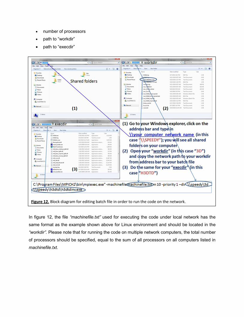
number of processors

path to “workdir”

path to “execdir”

In figure 12, the file “machinefile.txt” used for executing the code under local network has the

same format as the example shown above for Linux environment and should be located in the

“workdir”. Please note that for running the code on multiple network computers, the total number

of processors should be specified, equal to the sum of all processors on all computers listed in

machinefile.txt.

Figure 12. Block diagram for editing batch file in order to run the code on the network.

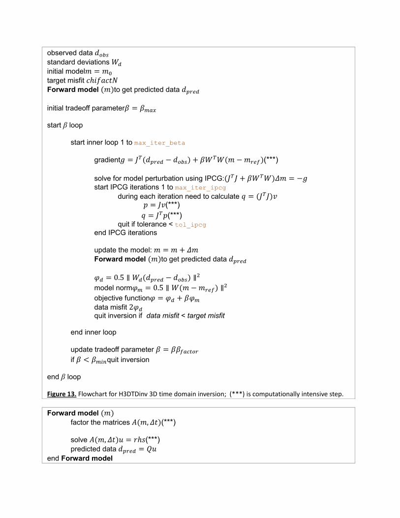
Inversion flowchart

The inversion flowchart is very similar to the inversion flowcharts for other UBC-GIF inversion

codes. The objective of the inversion is to minimize the objective function = d+m,

which is a combination of data misfit d and model norm m . d = Wd||dpred - dobs||2 and

should be in the range of the target misfit, equal to N*chifact, where N is the total number of

data from the data.dat file (excluding the dummy values) and chifact is 1 by default and can be

weighted to increase or decrease the desired target misfit. In the equation for d, Wd is the

standard deviation matrix (Wd = diag(1/SDi)), which is taken from the data.dat file and dpred is

the forward model field matrix, updated at every iteration step.

m is the model norm, which is used to regularize the objective function and is scaled to d

using the trade-off parameter . The model norm is a combination of model perturbation

functions m = (mi – mref), scaled using model weighting matrices Ws,x,y,z, which in turn, are

dependent on the user-defined smoothing parameters (’s). The inversion is driven by 3 levels

of iterative processes: the outer loop (minimizing the objective function), the beta-loop

(minimizing the trade-off parameter) and the IPCG loop, solving for the model perturbation m.

This model perturbation is used to calculate the forward model to get updated predicted data

(dpred). Other parameters and abbreviations listed in Figure 13 include:

J and JT – are the sensitivity matrix and the transposed sensitivity matrix respectively (J is a

measure of how sensitive is the model field to changes in electrical conductivities of the mesh

cells)

IPCG – Inexact Preconditioned Conjugate Gradient (a numerical method used to solve

minimization problems

g – gradient, calculated from the sensitivity matrix and used to solve for m

p, q, v – arbitrary vectors

The inversion is terminated if either the trade-off parameter becomes smaller that bmin, or the

objective function is minimized below the target misfit, or else if the maximum number of

iterations has been reached

observed data 𝑑𝑜𝑏𝑠

standard deviations 𝑊𝑑

initial model𝑚 = 𝑚0

target misfit 𝑐𝑕𝑖𝑓𝑎𝑐𝑡𝑁

Forward model (𝑚)to get predicted data 𝑑𝑝𝑟𝑒𝑑

initial tradeoff parameter𝛽 = 𝛽𝑚𝑎𝑥

start β loop

start inner loop 1 to max_iter_beta

gradient𝑔 = 𝐽𝑇(𝑑𝑝𝑟𝑒𝑑 − 𝑑𝑜𝑏𝑠) + 𝛽𝑊𝑇𝑊(𝑚 − 𝑚𝑟𝑒𝑓)(***)

solve for model perturbation using IPCG:(𝐽𝑇𝐽 + 𝛽𝑊𝑇𝑊)𝛥𝑚 = −𝑔

start IPCG iterations 1 to max_iter_ipcg

during each iteration need to calculate 𝑞 = (𝐽𝑇𝐽)𝑣

𝑝 = 𝐽𝑣(***)

𝑞 = 𝐽𝑇𝑝(***)

quit if tolerance < tol_ipcg

end IPCG iterations

update the model: 𝑚 = 𝑚 + 𝛥𝑚

Forward model (𝑚)to get predicted data 𝑑𝑝𝑟𝑒𝑑

𝜑𝑑 = 0.5 ∥ 𝑊𝑑(𝑑𝑝𝑟𝑒𝑑 − 𝑑𝑜𝑏𝑠) ∥2

model norm𝜑𝑚 = 0.5 ∥ 𝑊(𝑚 − 𝑚𝑟𝑒𝑓) ∥2

objective function𝜑 = 𝜑𝑑 + 𝛽𝜑𝑚

data misfit 2𝜑𝑑 quit inversion if data misfit < target misfit end inner loop

update tradeoff parameter 𝛽 = 𝛽𝛽𝑓𝑎𝑐𝑡𝑜𝑟

if 𝛽 < 𝛽𝑚𝑖𝑛quit inversion

end β loop

Figure 13. Flowchart for H3DTDinv 3D time domain inversion; (***) is computationally intensive step.

Forward model (𝑚)

factor the matrices 𝐴(𝑚, 𝛥𝑡)(***)

solve 𝐴(𝑚, 𝛥𝑡)𝑢 = 𝑟𝑕𝑠(***) predicted data 𝑑𝑝𝑟𝑒𝑑 = 𝑄𝑢

end Forward model

Output files

h3dtdinv.log - a log file showing the progress of the inversion. h3dtdinv.out - a file containing similar information as the log file, but arranged in a table. h3dtdinv_stat.txt - a file showing the factorizations and cpu time. inv_*.con - recovered model for each beta iteration. dpred_*.txt - predicted data for each beta iteration.