GVPCEW Page 1

GVP COLLEGE OF ENGINEERING FOR WOMEN

MADHURAWADA::VISAKHAPATNAM

Mathematical Optimization

Unit-I

Introduction to Operations Research

Objectives

Understand the meaning, purpose, and tools of Operations Research

Describe the history of Operations Research

Describe the Stages of O.R

Explain the Applications of Operations Research

Describe the Limitations of Operation Research

Formulate Linear Programming Problem

Solve the problem using graphical method

Definition: Operations Research

Operations Research has defined so far in various ways

Operations Research is a scientific method of providing executive departments with a quantitative basic for

decision regarding the operations under their control - Morse & Kimbal (1946)

Operations Research is a scientific method of providing executive with an analytical and objective basis for

decisions - PMS Blackett (1948)

Operations Research is the art of giving bad awareness to problems to which otherwise worse answers are

given - T.L.Saaty (1958)

Operations Research is concerned with scientifically deciding how best to design and operate man-machine

system usually under conditions requiring the allocation of scarce resources

-Operations Research Society of America

Operations Research is a method of mathematical based analysis for providing a quantitative basis for

management decisions.

Features of OR

1. Decision-Making: OR is addressed to managerial decision making or problem solving. A major

premise of OR is that decision making irrespective of the situation involved, can be considered as a

general systematic process.

2. Scientific Approach: OR employs scientific method for the purpose of solving problems. It is a

formalized process of reasoning.

GVPCEW Page 2

3. Objective: OR attempts to locate the best or optimal solution to the problem under consideration. For

this purpose, it is necessary that a measure of effectiveness is defined which is based on the goals of

the organization, this measure is then used as the basis to compare the alternative courses of action.

4. Inter-disciplinary team approach: OR is inter-disciplinary in nature and requires a team approach to a

solution of the problem. Managerial problems have economic, physical, psychological, biological,

sociological and engineering aspects. This requires a blend of people with expertise in the areas of

mathematics, statistics, engineering, economics, management, computer science, and so on.

5. Digital Computer: Use of a digital computer has become an integral part of the OR approach to

decision making. The computer may require due to the complexity of the model, volume of data

required and the computations to be made.

Modelling in Operations Research

A model is defined as a representation of an actual object or situation. It shows the relationships (direct or

indirect) and inter-relationships of action and reaction in terms of cause and effect. The main objective of a

model is to provide means for analysing the behaviour of the system for the purpose of improving its

performance or if a system is not in existence, then a model defines the ideal structure of this future system

indicating the functional relationships among its elements. The reliability of the solution obtained from a

model depends on the validity of the model in representing the real systems.

Models can be classified according the following characteristics

1. Classification by structure

a. Iconic models: Iconic models represent the system as it is by scaling it up or down.

Example: city maps, house blue prints, globe etc.

These models are easy to observe, build and describe but are difficult to manipulate and not very

useful for the purpose of prediction.

b. Analogue models: The models, in which one set of properties is used to represent another set of

properties, are called analogue models. These models are more abstract than the iconic ones for

there is no ‘look-like’ correspondence between these models and real life items.

Example: Graphs and maps in various colours are analogue models, in which different colours

correspond to different characteristics.

c. Symbolic (Mathematical) Models: The symbolic or Mathematical model is one which employs a

set of mathematical symbols to represent the decision variables of the system. These variables are

related together by means mathematical equation or a set of equations to describe the behaviour

of the system. These models are the easiest to manipulate experimentally and it is mst general

and abstract.

2. Classification by purpose

GVPCEW Page 3

Models can also be classified by purpose of its utility. The purpose of a model may be descriptive,

predictive or prescriptive.

a. Descriptive Models: A descriptive model simply describes some aspects of a situation based on

observations, survey, questionnaire result or other available data.

Example: The result of opinion poll represents a descriptive model.

b. Predictive Model: These models can answer ‘What if’ type of questions, i.e., they can make

predictions regarding certain events.

Example: Based on survey results, television networks attempt to explain and predict the election

results before all the votes are actually counted.

c. Prescriptive Models: When a predictive models has been repeatedly successful, it can be used to

prescribe a source of action.

Example: Linear programming is a prescriptive model because it prescribes what the managers

ought to do.

3. Classification by Nature of the Environment

a. Deterministic models: In these models, all the parameters and functional relationships are

assumed to be known with certainty when the decision is to be made.

Example: Linear Programming Problems, transportation and assignment models.

b. Probabilistic or Stochastic models: Models with atleast one parameter or decision variable is a

random variable is called probabilistic models. These models usually handle such situation in

which the consequences cannot be predicted with certainty. However it is possible to forecast a

pattern of events, based on which managerial decisions can be made.

Example: Insurance companies are willing to insure against risk fire, accidents etc., because the

pattern of events have been complied in the form of probability distributions.

4. Classification by behaviour

a. Static models: These models do not consider the impact of changes that takes place during the

planning horizon i.e. they are independent of time.

b. Dynamic models: In these models, time is considered as one of the important variables and

admits the impact of changes generated by time. In dynamic models, not only one but a series of

interdependent decisions is required during the planning horizon.

5. Classification by the method of solution

a. Analytical models: These models have a specific mathematical structure and thus can be solved

by known analytical or mathematical techniques.

b. Simulation models: These models also have a mathematical structure but they cannot be solved

by purely using the tools and techniques of mathematics. A simulation model is essentially

computer assisted experimentation to study the system under variety of assumptions.

GVPCEW Page 4

6. Classification by use of Digital computers

The development of the digital computers has led to the introduction of the following types of

modelling in OR

a. Analogue and Mathematical models combined: Sometimes analogue models are also expressed

in terms of mathematical symbols such models may belong to both analogue and mathematical

models.

b. Function models: These kinds of models are grouped based on the function being performed.

c. Quantitative models: These models are used to measure the observations.

d. Heuristic models: These models are mainly used to explore alternative strategies that were

overlooked previously. Heuristics models do not claim to find the best solution to the problem.

Methodology of Operations Research

The methodology to be adopted involves the following phases

1. Formulation of the problem:

The following information will be required to formulate the problem

(i) Who has to take the decision?

(ii) What are the objectives?

(iii) What are the ranges of controlled variable?

(iv) What are the uncontrolled variables that may affect the possible solutions?

(v) What are the restrictions or constraints on the variables

Since wrong formulation can’t yield a right decision, one must be considerably careful while executing

this phase.

2. Constructing a mathematical model:

After formulation of the problem, the next step is to express all the relevant variables of the problem into

mathematical model. A mathematical model should include three important basic factors

(i) Decision variables and parameters

(ii) Constraints

(iii) Objective function

3. Deriving the solution from the model

This phase is devoted to the computation of those values of decision variables that optimize the objective

function; such solution is called an optimal solution which is always in the best interest of the problem

under consideration.

4. Testing the model and its solution

After the construction of the model, it is once again tested as a whole for the errors if any. A model may

be said to be valid, if it can provide a reliable prediction of the system’s performance. A good model

GVPCEW Page 5

may be applicable for a longer time and thus updates the model time to time by taking into account the

past, present and future specifications of the problem.

5. Controlling the solution

This phase establishes control over the solution. The model requires immediate modification as soon as

the controlled variables changes significantly otherwise the model goes out of control.

6. Implementing the solution

Finally, the tested results of the model are implemented to work. This phase is primarily executed with

the cooperation of OR experts and those who are responsible for managing and operating the systems.

O.R. Tools and Techniques

Operations Research has many suitable tools/techniques which can be used for problem solving. The

common used tools/techniques are:

1. Linear Programming: This is a constrained optimization technique, which optimize some criterion within

some constraints. In Linear programming the objective function (profit, loss or return on investment) and

constraints are linear. There are different methods available to solve linear programming.

2. Game Theory: This is used for making decisions under conflicting situations where there are one or

more players/opponents. In this the motive of the players are dichotomized. The success of one player

tends to be at the cost of other players and hence they are in conflict.

3. Decision Theory: Decision theory is concerned with making decisions under conditions of complete

certainty about the future outcomes and under conditions such that we can make some probability about

what will happen in future.

4. Queuing Theory: This is used in situations where the queue is formed (for example customers waiting

for service, aircrafts waiting for landing, jobs waiting for processing in the computer system, etc). The

objective here is minimizing the cost of waiting without increasing the cost of servicing.

5. Inventory Models: Inventory model make a decisions that minimize total inventory cost. This model

successfully reduces the total cost of purchasing, carrying, and out of stock inventory.

6. Simulation: Simulation is a procedure that studies a problem by creating a model of the process involved

in the problem and then through a series of organized trials and error solutions attempt to determine the

best solution. Sometimes this is a difficult/time consuming procedure. Simulation is used when actual

experimentation is not feasible or solution of model is not possible.

7. Non-linear Programming: This is used when the objective function and the constraints are not linear in

nature. Linear relationships may be applied to approximate non-linear constraints but limited to some

range, because approximation becomes poorer as the range is extended. Thus, the non-linear

programming is used to determine the approximation in which a solution lies and then the solution is

obtained using linear methods.

GVPCEW Page 6

8. Dynamic Programming: Dynamic programming is a method of analyzing multistage decision processes.

In this each elementary decision depends on those preceding decisions and as well as external factors.

9. Integer Programming: If one or more variables of the problem take integral values only then dynamic

programming method is used. For example number or motor in an organization, number of passenger in

an aircraft, number of generators in a power generating plant, etc.

10. Markov Process: Markov process permits to predict changes over time information about the behaviour

of a system is known. This is used in decision making in situations where the various states are defined.

The probability from one state to another state is known and depends on the current state and is

independent of how we have arrived at that particular state.

11. Network Scheduling: This technique is used extensively to plan, schedule, and monitor large projects

(for example computer system installation, R & D design, construction, maintenance, etc.). The aim of

this technique is minimize trouble spots (such as delays, interruption, production bottlenecks, etc.) by

identifying the critical factors. The different activities and their relationships of the entire project are

represented diagrammatically with the help of networks and arrows, which is used for identifying critical

activities and path. There are two main types of technique in network scheduling, they are: Program

Evaluation and Review Technique (PERT) – is used when activities time is not known accurately/ only

probabilistic estimate of time is available. Critical Path Method (CPM) – is used when activities time is

known accurately.

12. Information Theory: This analytical process is transferred from the electrical communication field to

O.R. field. The objective of this theory is to evaluate the effectiveness of flow of information with a

given system. This is used mainly in communication networks but also has indirect influence in

simulating the examination of business organizational structure with a view of enhancing flow of

information.

Applications of Operations Research

OR is mainly concerned with the techniques of applying scientific knowledge, besides the development of

science. It provides an understanding which gives the expert/manager new insights and capabilities to

determine better solutions in decision making problems with great speed, competence and confidence. In

recent years, OR has entered successfully in many different areas of research for defence, government and

industry. There are voluminous of applications of Operations Research. The following are the set of typical

operations research applications to show how widely these techniques are used today:

Accounting:

Assigning audit teams effectively

Credit policy analysis

Cash flow planning

Developing standard costs

GVPCEW Page 7

Establishing costs for byproducts

Planning of delinquent account strategy

Agriculture:

Allocation lands to various crops according to climatic conditions.

Optimum distribution of water

Construction:

Project scheduling, monitoring and control

Determination of proper work force

Deployment of work force

Allocation of resources to projects

Facilities Planning:

Factory location and size decision

Estimation of number of facilities required

Hospital planning

International logistic system design

Transportation loading and unloading

Warehouse location decision

Finance:

Building cash management models

Allocating capital among various alternatives

Building financial planning models

Investment analysis

Portfolio analysis

Dividend policy making

Manufacturing:

Inventory control

Marketing balance projection

Production scheduling

Production smoothing

Marketing:

Advertising budget allocation

Product introduction timing

Selection of Product mix

Deciding most effective packaging alternative

Organizational Behavior / Human Resources:

GVPCEW Page 8

Personnel planning

Recruitment of employees

Skill balancing

Training program scheduling

Designing organizational structure more effectively

Purchasing:

Optimal buying

Optimal reordering

Materials transfer

Research and Development:

R & D Projects control

R & D Budget allocation

Planning of Product introduction

Limitations of Operations Research

Operations Research has number of applications; similarly it also has certain limitations. These limitations

are mostly related to the model building and money and time factors problems involved in its application.

Some of them are as given below:

1. There are certain problems which a decision maker may have to solve only once. Constructing a

complex OR model for solving such problems is often too expensive when compared with the cost of

other less sophisticated approaches available to solve them.

2. Sometimes OR specialists become too much enamoured with the model they have built and forget

the fact that their model does not represent the ‘real world problem’ in which decisions have to be

made.

3. Sometimes the basic data are subject to frequent changes. In such cases, modification of OR model is

a costly affair.

4. Many OR models are so complex that they can’t be solved without the use of computer. Also, the

solutions obtained from these models are difficult to explain to managers and hence fail to gain their

support and confidence.

5. Magnitude of the computations involved, lack of consideration for non-quantifiable factors and

psychological issues involved in implementation are some of the other short comings of OR.

Linear Programming -I

The Linear Programming Problem (LPP) calls for optimizing a linear function of variables called the

objective function subject to a set of linear equations and/or inequalities called constraints.

Mathematical formulation of LP model:

GVPCEW Page 9

1. Study the given situation; find the key decisions to be made. Hence identify the decision variables of

the problem.

2. Formulate the objective function to be optimized.

3. Identify constraints of the problem and express them as linear equation or inequality.

4. State the feasible alternatives (generally𝑥𝑗 ≥ 0 ∀𝑗).

The objective function, the set of constraints and non-negativity restrictions together form an LP model.

Example 1: Suppose an industry is manufacturing two types of products P1 and P2. The profits per Kg of

the two products are Rs.30 and Rs.40 respectively. These two products require processing in three types of

machines. The following table shows the available machine hours per day and the time required on each

machine to produce one Kg of P1 and P2. Formulate the problem in the form of linear programming model.

Profit/Kg P1

Rs.30

P2

Rs.40

Total available Machine

hours/day

Machine 1 3 2 600

Machine 2 3 5 800

Machine 3 5 6 1100

Solution:

The procedure for linear programming problem formulation is as follows:

Introduce the decision variable as follows:

Let x1 = amount of P1

x2 = amount of P2

In order to maximize profits, we establish the objective function as

30x1 + 40x2

Since one Kg of P1 requires 3 hours of processing time in machine 1 while the corresponding

requirement of P2 is 2 hours. So, the first constraint can be expressed as

3x1 + 2x2 ≤ 600

Similarly, corresponding to machine 2 and 3 the constraints are

3x1 + 5x2 ≤ 800

5x1 + 6x2 ≤ 1100

In addition to the above there is no negative production, which may be represented algebraically as

x1 ≥ 0 ; x2 ≥ 0

Thus, the product mix problem in the linear programming model is as follows:

Maximize 30x1 + 40x2

GVPCEW Page 10

Subject to:

3x1 + 2x2 ≤ 600

3x1 + 5x2 ≤ 800

5x1 + 6x2 ≤ 1100

x1≥ 0, x2 ≥ 0

Example 2: A company owns two flour mills viz. A and B, which have different production capacities for

high, medium and low quality flour. The company has entered a contract to supply flour to a firm every

month with at least 8, 12 and 24 quintals of high, medium and low quality respectively. It costs the company

Rs.2000 and Rs.1500 per day to run mill A and B respectively. On a day, Mill A produces 6, 2 and 4quintals

of high, medium and low quality flour, Mill B produces 2, 4 and 12 quintals of high, medium and low

quality flour respectively. How many days per month should each mill be operated in order to meet the

contract order most economically.

Solution:

Let us define x1 and x2 are the mills A and B. Here the objective is to minimize the cost of the machine

runs and to satisfy the contract order. The linear programming problem is given by

Minimize 2000x1 + 1500x2

Subject to:

6x1 + 2x2 ≥ 8

2x1 + 4x2 ≥ 12

4x1 + 12x2 ≥ 24

x1 ≥ 0, x2 ≥ 0

Graphical Method of Solving LPP

A two variable linear programming problem can be easily solved graphically. The method is simple but the

principle of solution is depends on certain analytical concepts, they are:

The major steps in the solution of LPP by graphical method are:

Step 1: Identify the problem – the decision variables, the objective and the constraints.

Step 2: Set up the mathematical formulation of the problem.

Step3: Plot a graph representing all the constraints of the problem and identify the feasible region (solution

space). The feasible region is the intersection of all the regions represented by the constraints of the problem

and is restricted to the first quadrant only.

Step 4: The feasible region obtained in step 3 may be bounded or unbounded. Compute the coordinates of all

the corner points of the feasible region.

Step 5: Find out the value of the objective function at each corner point determined in step 4.

Step 6: Select the corner point that optimizes the value of the objective function, it gives the optimum

feasible solution.

GVPCEW Page 11

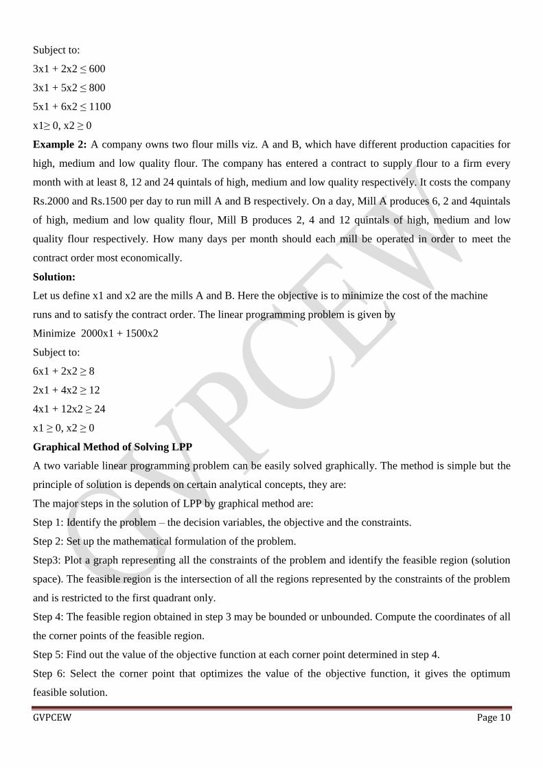
Example 1: Solve the LPP using Graphical Method

Maximize 30𝑥1 + 40𝑥2

Subject to: 3𝑥1 + 2𝑥2 ≤ 600; 3𝑥1 + 5𝑥2 ≤ 800; 5𝑥1 + 6𝑥2 ≤ 1100; 𝑥1 ≥ 0, 𝑥2 ≥ 0

The extreme point of this convex region are O, A, B, C and D.

The optimal value of the objective function occurs at one of the corner points of the feasible region

Extreme Point Coordinates Objective function

O (0, 0) 0

A (0, 160) 6400

B (110, 70) 6100

C (170, 40) 6700

D (200, 0) 6000

The optimum value variables are 𝑥1 = 170 and 𝑥2 = 40.

Example 2: Solve the LPP using Graphical Method

Minimize 2000𝑥1 + 1500𝑥2

Subject to:

6𝑥1 + 2𝑥2 ≥ 8 ; 2𝑥1 + 4𝑥2 ≥ 12; 4𝑥1 + 12𝑥2 ≥ 24

𝑥1 ≥ 0, 𝑥2 ≥ 0

Extreme Point Coordinates Objective function

GVPCEW Page 12

A (0, 4) 6000

B (0.5 2.75) 5125

C (6, 0) 12000

The objective is minimum at B(0.5, 2.75)

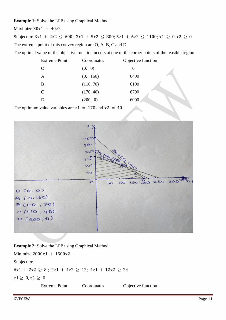
Example 3: Solve the LPP using graphical method

Maximize 3𝑥1 + 𝑥2

Subject to: 𝑥1 + 𝑥2 ≥ 6; −𝑥1 + 𝑥2 ≤ 6; −𝑥1 + 2𝑥2 ≥ −6

and 𝑥1, 𝑥2 ≥ 0

GVPCEW Page 13

No fesible solution exists.