Guy Barles, Olivier Ley, Thi-Tuyen Nguyen, Thanh Phan

HAL Id: hal-01592608https://hal.archives-ouvertes.fr/hal-01592608v2

Submitted on 22 May 2018

HAL is a multi-disciplinary open accessarchive for the deposit and dissemination of sci-entific research documents, whether they are pub-lished or not. The documents may come fromteaching and research institutions in France orabroad, or from public or private research centers.

L’archive ouverte pluridisciplinaire HAL, estdestinée au dépôt et à la diffusion de documentsscientifiques de niveau recherche, publiés ou non,émanant des établissements d’enseignement et derecherche français ou étrangers, des laboratoirespublics ou privés.

Large time behavior of unbounded solutions offirst-order Hamilton-Jacobi equations in RN

Guy Barles, Olivier Ley, Thi-Tuyen Nguyen, Thanh Phan

To cite this version:Guy Barles, Olivier Ley, Thi-Tuyen Nguyen, Thanh Phan. Large time behavior of unbounded solutionsof first-order Hamilton-Jacobi equations in RN . Asymptotic Analysis, IOS Press, 2019, 112 (1-2),pp.1-22. 10.3233/ASY-181488. hal-01592608v2

https://hal.archives-ouvertes.fr/hal-01592608v2

https://hal.archives-ouvertes.fr

LARGE TIME BEHAVIOR OF UNBOUNDED SOLUTIONS OFFIRST-ORDER HAMILTON-JACOBI EQUATIONS IN THE

WHOLE SPACE

GUY BARLES, OLIVIER LEY, THI-TUYEN NGUYEN, AND THANH VIET PHAN

Abstract. We study the large time behavior of solutions of first-order con-vex Hamilton-Jacobi Equations of Eikonal type set in the whole space. Weassume that the solutions may have arbitrary growth. A complete study of thestructure of solutions of the ergodic problem is provided : contrarily to the pe-riodic setting, the ergodic constant is not anymore unique, leading to differentlarge time behavior for the solutions. We establish the ergodic behavior of thesolutions of the Cauchy problem (i) when starting with a bounded from be-low initial condition and (ii) for some particular unbounded from below initialcondition, two cases for which we have different ergodic constants which play arole. When the solution is not bounded from below, an example showing thatthe convergence may fail in general is provided.

1. Introduction

This work is concerned with the large time behavior for unbounded solutionsof the first-order Hamilton-Jacobi equation

ut(x, t) +H(x,Du(x, t)) = l(x), in RN × (0,+∞),

u(·, 0) = u0(·) in RN ,(1.1)

where H ∈ W 1,∞loc (RN × RN) satisfies

There exists ν ∈ C(RN), ν > 0 such that H(x, p) ≥ ν(x)|p|,(1.2)

0 = H(x, 0) < H(x, p) for p 6= 0,(1.3)

H(x, ·) is convex,(1.4)

There exist a constant CH > 0 and, for all R > 0, a constant kR such that

|H(x, p)−H(y, q)| ≤ kR(1 + |p|)|x− y|+ CH |p− q|,(1.5)

for all |x|, |y| ≤ R, p, q ∈ RN .

We always assume u0, l ∈ C(RN) and

l ≥ 0 in RN .(1.6)

2010 Mathematics Subject Classification. Primary 35F21; Secondary 35B40, 35Q93, 49L25.Key words and phrases. Hamilton-Jacobi equations; asymptotic behavior; ergodic problem;

unbounded solutions; viscosity solutions.1

2 G. BARLES, O. LEY, T.-T. NGUYEN, T. V. PHAN

These assumptions are those used in the so-called Namah-Roquejoffre case intro-duced in [25] in the periodic case, and in Barles-Roquejoffre [4] in the unboundedcase. They are not the most general but, for simplicity, we choose to state asabove since they are well-designed to encompass the classical Eikonal equation

(1.7) ut(x, t) + a(x)|Du(x, t)| = l(x), in RN × (0,+∞),

where a(·) is a locally Lipschitz, bounded function such that a(x) > 0 in RN . Theassumption (1.2) is a coercivity assumption, which may be replaced by (2.2). Wealso may replace (1.6) by l is bounded from below up to assume that H(x, 0) −infRN l = 0 in (1.3).

Our goal is to prove that, under suitable additional assumptions, there existsa unique viscosity solution u of (1.1) and that this solution satisfies

u(x, t) + ct→ v(x) in C(RN) as t→ +∞,

where (c, v) ∈ R+ × C(RN) is a solution to the ergodic problem

H(x,Dv(x)) = l(x) + c in RN .(1.8)

This problem has not been widely studied comparing to the periodic case [13,25, 5, 14, 12, 6, 1] and references therein. The main works in the unboundedsetting are Barles-Roquejoffre [4] which extends the well-known periodic resultof Namah-Roquejoffre [25], the works of Ishii [21] and Ichihara-Ishii [18]. A veryinteresting reference is the review of Ishii [22]. We will compare more preciselyour results with the existing ones below but let us mention that our main goalis to make more precise the large time behavior for the Eikonal Equation (1.7)in a setting where the equation is well-posed for solutions with arbitrary growth,which brings delicate issues. Most of our results were already obtained or areclose to results of [4, 18] but we use pure PDE arguments to prove them withoutusing Weak KAM methods and making a priori assumptions on the structure ofsolutions or subsolutions of (1.8).

Changing u(x, t) in u(x, t) − infRNlt allows to reduce to the case wheninfRN l = 0 and we are going to actually reduce to that case to simplify theexposure. Taking this into account, we use below the assumption

lim inf|x|→+∞

l(x) > infRN

(l) = 0.(1.9)

which is a compactness assumption in the sense that it implies

A := argmin l = x ∈ RN : l(x) = 0 is a nonempty compact subset of RN .

This subset corresponds to the Aubry set in the framework of Weak KAM theory.Our first main result collects all the properties we obtain for the solutions

of (1.8).

LARGE TIME BEHAVIOR OF UNBOUNDED SOLUTIONS 3

Theorem 1.1. (Ergodic problem)Assume that 0 ≤ l ∈ C(RN) and H ∈ C(RN × RN).

(i) If H satisfies (1.2) and H(x, 0) = 0 for all x ∈ RN then, for all c ≥ 0, thereexists a solution (c, v) ∈ R+ ×W 1,∞

loc (RN) of (1.8).

(ii) Assume that (1.1) satisfies a comparison principle in C(RN × [0,+∞)). If(c, v) and (d, w) are solutions of (1.8) with supRN |v − w| <∞, then c = d.

(iii) If A 6= ∅ and H satisfies (1.2) and (1.3), then there exists a solution (c, v) ∈R+ ×W 1,∞

loc (RN) of (1.8) with c = 0 and v ≥ 0. If, in addition,

H(x, p) ≤ m(|p|) for some increasing function m ∈ C(R+,R+),(1.10)

and A satisfies (1.9), then v(x)→ +∞ as |x| → ∞.(iv) Let c > 0. If H satisfies (1.10) then any solution (c, v) of (1.8) is unboundedfrom below. If H satisfies H(x, 0) = 0 and (1.4) and (c, v), (c, w) are two solutionsof (1.8) with v(x)− w(x)→ 0 as |x| → ∞, then v = w.

The situation is completely different with respect to the periodic setting wherethere is a unique ergodic constant (or critical value) for which (1.8) has a solution(e.g., Lions-Papanicolaou-Varadhan [24] or Fathi-Siconolfi [15]). We recover someresults of Barles-Roquejoffre [4] and Fathi-Maderna [16], see Remark 2.3 for adiscussion. As far as the case of unbounded solutions of elliptic equations isconcerned, let us mention the recent work of Barles-Meireles [7] and the referencestherein.

Coming back to (1.1), when H satisfies (1.5), we have a comparison principle bya “finite speed of propagation” type argument, which allows to compare sub- andsupersolutions without growth condition ([19, 23] and Theorem A.1). It followsthat there exists a unique continuous solution defined for all time as soon as thereexist a sub- and supersolution.

Proposition 1.2. Assume that l ≥ 0 and H satisfies (1.2) and (1.5). Let u0 ∈C(RN) and c ≥ 0.

(i) There exists a smooth supersolution (c, v+) of (1.8) satisfying u0 ≤ v+ in RN .

(ii) If there exists a subsolution (c, v−) of (1.8) satisfying v− ≤ u0 in RN , thenthere exists a unique viscosity solution u ∈ C(RN × [0,+∞)) of (1.1) such that

v−(x) ≤ u(x, t) + ct ≤ v+(x) for all (x, t) ∈ RN × [0,+∞).(1.11)

Notice that the existence of a subsolution is given by (1.3) for instance.

We give two convergence results depending on the critical value c = 0 or c > 0.

Theorem 1.3. (Large time behavior starting with bounded from below initialdata) Assume (1.2)-(1.3)-(1.4)-(1.5), l ≥ 0, and (1.9). Then, for every boundedfrom below initial data u0, the unique viscosity solution u of (1.1) satisfies

u(x, t) →t→+∞

v(x) locally uniformly in RN ,(1.12)


where (0, v) is a solution to (1.8).

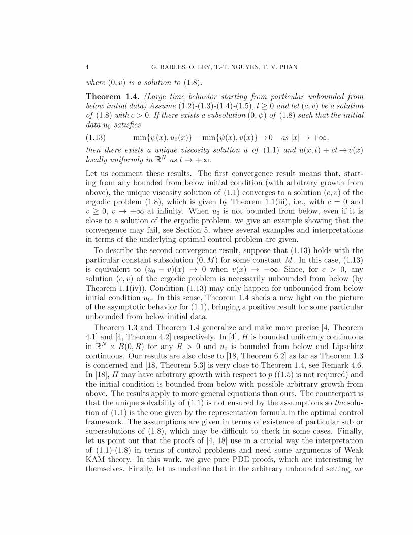
Theorem 1.4. (Large time behavior starting from particular unbounded frombelow initial data) Assume (1.2)-(1.3)-(1.4)-(1.5), l ≥ 0 and let (c, v) be a solutionof (1.8) with c > 0. If there exists a subsolution (0, ψ) of (1.8) such that the initialdata u0 satisfies

minψ(x), u0(x) −minψ(x), v(x)→ 0 as |x| → +∞,(1.13)

then there exists a unique viscosity solution u of (1.1) and u(x, t) + ct→ v(x)locally uniformly in RN as t→ +∞.

Let us comment these results. The first convergence result means that, start-ing from any bounded from below initial condition (with arbitrary growth fromabove), the unique viscosity solution of (1.1) converges to a solution (c, v) of theergodic problem (1.8), which is given by Theorem 1.1(iii), i.e., with c = 0 andv ≥ 0, v → +∞ at infinity. When u0 is not bounded from below, even if it isclose to a solution of the ergodic problem, we give an example showing that theconvergence may fail, see Section 5, where several examples and interpretationsin terms of the underlying optimal control problem are given.

To describe the second convergence result, suppose that (1.13) holds with theparticular constant subsolution (0,M) for some constant M . In this case, (1.13)is equivalent to (u0 − v)(x) → 0 when v(x) → −∞. Since, for c > 0, anysolution (c, v) of the ergodic problem is necessarily unbounded from below (byTheorem 1.1(iv)), Condition (1.13) may only happen for unbounded from belowinitial condition u0. In this sense, Theorem 1.4 sheds a new light on the pictureof the asymptotic behavior for (1.1), bringing a positive result for some particularunbounded from below initial data.

Theorem 1.3 and Theorem 1.4 generalize and make more precise [4, Theorem4.1] and [4, Theorem 4.2] respectively. In [4], H is bounded uniformly continuousin RN × B(0, R) for any R > 0 and u0 is bounded from below and Lipschitzcontinuous. Our results are also close to [18, Theorem 6.2] as far as Theorem 1.3is concerned and [18, Theorem 5.3] is very close to Theorem 1.4, see Remark 4.6.In [18], H may have arbitrary growth with respect to p ((1.5) is not required) andthe initial condition is bounded from below with possible arbitrary growth fromabove. The results apply to more general equations than ours. The counterpart isthat the unique solvability of (1.1) is not ensured by the assumptions so the solu-tion of (1.1) is the one given by the representation formula in the optimal controlframework. The assumptions are given in terms of existence of particular sub orsupersolutions of (1.8), which may be difficult to check in some cases. Finally,let us point out that the proofs of [4, 18] use in a crucial way the interpretationof (1.1)-(1.8) in terms of control problems and need some arguments of WeakKAM theory. In this work, we give pure PDE proofs, which are interesting bythemselves. Finally, let us underline that in the arbitrary unbounded setting, we


do not have in hands local Lipschitz bounds, i.e. bounds on |ut|, |Du| ≤ C, withC independent of t. These bounds are easy consequences of the coercivity of H inthe periodic setting and in the Lipschitz setting of [4]. In the general unboundedcase, such bounds require additional restrictive assumptions. Instead, we providea more involved proof without further assumptions, see the proof of Theorem 1.3.

Let us also mention that several other convergence results are established in [21]and [18] in the case of strictly convex Hamiltonian H and [17] is devoted to aprecise study in the one dimensional case. We refer again the reader to thereview [22] for details and many examples.

The paper is organized as follows. We start by solving the ergodic prob-lem (1.8), see Section 2. Then, we consider the evolution problem (1.1) inSection 3. Section 4 is devoted to the proofs of the theorems of convergence.Finally, Section 5 provides several examples based both on the Hamilton-Jacobiequations (1.1)-(1.8) and on the associated optimal control problem.

Acknowledgements: Part of this work was made during the stay of T.-T.Nguyen as a Ph.D. student at IRMAR and she would like to thank University ofRennes 1 & INSA for the hospitality. The work of O. Ley and T.-T. Nguyen waspartially supported by the Centre Henri Lebesgue ANR-11-LABX-0020-01. Theauthors would like to thank the referees for the careful reading of the manuscriptand their useful comments.

2. The Ergodic problem

Before giving the proof of Theorem 1.1, we start with a lemma based on thecoercivity of H.

Lemma 2.1. Let Ω ⊂ RN be an open bounded subset and H satisfies (1.2). Forevery subsolution (c, v) ∈ R+ × USC(Ω) of (1.8), we have v ∈ W 1,∞(Ω) and

|Dv(x)| ≤ maxy∈Ω

l(y) + c

ν(y)

for a.e. x ∈ Ω.(2.1)

Remark 2.2. Assumption (1.2) was stated in that way having in mind the EikonalEquation (1.7) but it can be replaced by the classical assumption of coercivity

lim|p|→+∞

infx∈B(0,R)

H(x, p) = +∞ for all R > 0.(2.2)

Proof of Lemma 2.1. Let B(x0, R) be any ball contained in Ω. Since v is a vis-cosity subsolution of


l(y) + c

ν(y)

in Ω,


we see from [1, Proposition 1.14, p.140] that v is Lipschitz continuous in B(x0, R)with the Lipschitz constant maxΩ

l+cν

, which implies together with Rademacher

theorem


l(y) + c

ν(y)

for a.e. x ∈ B(x0, R).

We are now able to give the proof of Theorem 1.1.

Proof of Theorem 1.1.

(i) We follow some arguments of the proof of [4, Theorem 2.1]. Fix c ≥ 0, noticingthat l(x) + c ≥ 0 for every x ∈ RN and recalling that H(x, 0) = 0, we infer that0 is a subsolution of (1.8). For R > 0, we consider the Dirichlet problem

H(x,Dv) = l(x) + c in B(0, R), v = 0 on ∂B(0, R).(2.3)

If pR ∈ RN and CR > 0, |pR| are big enough, then, using (1.2), CR + 〈pR, x〉 isa supersolution of (2.3). By Perron’s method up to the boundary ([11, Theorem6.1]), the function

VR(x) := supv ∈ USC(B(0, R)) subsolution of (2.3) :

0 ≤ v(x) ≤ CR + 〈pR, x〉 for x ∈ B(0, R),

is a discontinuous viscosity solution of (2.3). Recall that the boundary conditionsare satisfied in the viscosity sense meaning that either the viscosity inequality orthe boundary condition for the semicontinuous envelopes holds at the boundary.We claim that VR ∈ W 1,∞(B(0, R)) and VR(x) = 0 for every x ∈ ∂B(0, R),i.e., the boundary conditions are satisfied in the classical sense. At first, fromLemma 2.1, VR ∈ W 1,∞(B(0, R)). By definition, VR ≥ 0 in B(0, R), so (VR)∗ ≥0 on ∂B(0, R) and the boundary condition holds in the classical sense for thesupersolution. It remains to check that (VR)∗ ≤ 0 on ∂B(0, R). We argue bycontradiction assuming there exists x ∈ ∂B(0, R) such that (VR)∗(x) > 0. Itfollows that the viscosity inequality for subsolutions holds at x, i.e., for everyϕ ∈ C1(B(0, R)) such that ϕ ≥ (VR)∗ over B(0, R) with (VR)∗(x) = ϕ(x), wehave H(x, Dϕ(x)) ≤ l(x) + c and there exists at least one such ϕ. Consider, forK > 0, ϕ(x) := ϕ(x) −K〈 x|x| , x − x〉. We still have ϕ ≥ (VR)∗ over B(0, R) and

(VR)∗(x) = ϕ(x). Therefore H(x, Dϕ(x)−K x|x|) ≤ l(x)+c for every K > 0, which

is absurd for large K by (1.2). It ends the proof of the claim.We set vR(x) = VR(x)− VR(0). By Lemma 2.1, for every R > R′, we have

|DvR(x)| = |DVR(x)| ≤ CR′ := maxB(0,R′)

l + c

ν

a.e. x ∈ B(0, R′),(2.4)

|vR(x)| = |VR(x)− VR(0)| ≤ CR′R′ for x ∈ B(0, R′).(2.5)


Up to an extraction, by Ascoli’s Theorem and a diagonal process, vR converges inC(RN) to a function v as R → +∞, which still satisfies (2.4)-(2.5). By stabilityof viscosity solutions, (c, v) is a solution of (1.8).

(ii) Let (c, v) and (d, w) be two solutions of (1.8) and set

V (x, t) = v(x)− ctW (x, t) = w(x)− dt.

To show that c = d, we argue by contradiction, assuming that c < d. Obviously,V is a viscosity solution of (1.1) with u0 = v and W is a viscosity solution of (1.1)with u0 = w. Using the comparison principle for (1.1), we get that

V (x, t)−W (x, t) ≤ supRN

v − w for all (x, t) ∈ RN × [0,∞).

This means that

(d− c)t+ v(x)− w(x) ≤ supRN

v − w for all (x, t) ∈ RN × [0,∞).

Recalling that supRN |v − w| <∞, we get a contradiction for t large enough. Byexchanging the roles of v, w, we conclude that c = d.

(iii) Let c = 0. We apply the Perron’s method using in a crucial way A 6= ∅. LetS = w ∈ USC(RN) subsolution of (1.8) : 0 ≤ w and w = 0 on A and set

v(x) := supw∈S

w(x).

Noticing that l + c ≥ 0 and since H(x, 0) = 0, we have 0 ∈ S. Let x ∈ RN andR > 0 large enough such that x ∈ B(0, R) and there exists xA ∈ B(0, R) ∩ A.For all w ∈ S, by Lemma 2.1, we have

0 ≤ w(x) ≤ w(xA) + maxB(0,R)

l + c

ν

|x− xA| ≤ 2R max

B(0,R)

l + c

ν

,

since w(xA) = 0. The above upper-bound does not depend on w ∈ S, so wededuce that 0 ≤ v(x) < +∞ for every x ∈ RN .

We claim that v is a solution of (1.8). At first, by classical arguments ([3]),v is still a subsolution of (1.8) satisfying v ≥ 0 in RN and v = 0 on A. ByLemma 2.1, v ∈ W 1,∞

loc (RN). To prove that v is a supersolution, we argue asusual by contradiction assuming that there exists x and ϕ ∈ C1(RN) such thatϕ ≤ v, v(x) = ϕ(x) and the viscosity supersolution inequality does not hold, i.e.,H(x, Dϕ(x)) < l(x) + c. To reach a contradiction, one slightly modify v near xin order to build a new subsolution v in S, which is strictly bigger than v near x.To be able to proceed as in the classical proof, it is enough to check that x 6∈ A;otherwise v will not be 0 on A leading to v 6∈ S. If x ∈ A, then l(x) + c = 0.By (1.3), we obtain 0 ≤ H(x, Dϕ(x)) < l(x) + c = 0, which is not possible. Itends the proof of the claim.


From (1.9), there exists εA, RA > 0 such that l(x) > minRN l + εA for allx ∈ RN \B(0, RA). By (1.10), v satisfies, in the viscosity sense

m(|Dv|) ≥ H(x,Dv) ≥ l(x) + c ≥ εA in RN \B(0, RA).

Therefore, for all x ∈ RN and every p in the viscosity subdifferential D−v(x) of vat x, we have |p| ≥ m−1(εA) > 0. By the viscosity decrease principle [23, Lemma4.1], for all B(x,R) ⊂ RN \B(0, RA), we obtain

infB(x,R)

v ≤ v(x)−m−1(εA)R.

Since v ≥ 0, for any R > 0 and x such that |x| > RA + R, we conclude v(x) ≥m−1(εA)R, which proves that v(x)→ +∞ as |x| → +∞.(iv) Since c > 0, there exists α > 0 such that l(x) + c ≥ α for all x ∈ RN .

To prove that v is unbounded from below, we use again the viscosity decreaseprinciple [23, Lemma 4.1]. By (1.10), v satisfies, in the viscosity sense

m(|Dv|) ≥ H(x,Dv) ≥ α in RN ,

which implies, for all R > 0,

infB(0,R)

v ≤ v(0)−m−1(α)R

and so v cannot be bounded from below.For the second part of the result, we argue by contradiction assuming that

v 6= w. Without loss of generality, there exists η > 0 and x ∈ RN such that(v−w)(x) > 3η. Since (v−w)(x)→ 0 as |x| → +∞, there exists R > 0 such that|(v − w)(x)| < η when |x| ≥ R. Up to choose 0 < µ < 1 sufficiently close to 1,we have |(µv−w)(x)| > 2η and, by compactness of ∂B(0, R), |(µv−w)(x)| < 2ηfor all x ∈ ∂B(0, R). It follows that M := maxB(0,R) µv − w cannot be achieved

at the boundary of B(0, R). Consider

Mε := maxx,y∈B(0,R)

µv(x)− w(y)− |x− y|

2

ε2

,

which is achieved at some (x, y). By classical properties ([2, 3]), up to extractsome subsequences ε→ 0,

|x− y|2

ε2→ 0,

x, y → x0 for some x0 ∈ B(0, R),

Mε →M.

It follows that M = (µv − w)(x0) and therefore, for ε small enough, neither xnor y is on the boundary of B(0, R). We can write the viscosity inequalities for v


subsolution at x and w supersolution at y for small ε leading to

H(x,p

µ) ≤ l(x) + c,

H(y, p) ≥ l(y) + c,

where we set p = 2(x− y)

ε2. Noticing that

µv(x)− w(x) ≤ µv(x)− w(y)− |x− y|2

ε2

and using that w is Lipschitz continuous with some constant CR in B(0, R) byLemma 2.1, we obtain |p| ≤ CR. Therefore, up to extract a subsequence ε → 0,we have p→ p0. By the convexity of H,

H(x, p) = H(x, µp

µ+ (1− µ)0) ≤ µH(x,

p

µ) + (1− µ)H(x, 0).

Using H(x, 0) = 0, we get

0 ≤ µH(x,p

µ)−H(x, p).

Subtracting the viscosity inequalities and using the above estimates, we obtain

0 ≤ µH(x,p

µ)−H(x, p) ≤ H(y, p)−H(x, p) + µ(l(x) + c)− (l(y) + c).

Sending ε → 0, we reach 0 ≤ (µ − 1)(l(x0) + c) ≤ (µ − 1)α < 0, which is acontradiction. It ends the proof of the theorem.

Remark 2.3.(i) In the periodic setting, there is a unique c = 0 such that (1.8) has a solution. Itis not anymore the case in the unbounded setting where there exist solutions forall c ≥ 0. The proof is adapted from [4, Theorem 2.1]. Similar issues are studiedin [16]. Notice that, when c < 0, there is no subsolution (thus no solution)because of (1.3).(ii) In the periodic setting, the classical proof of existence of a solution to (1.8)([24]) uses the auxiliary approximate equation

λvλ +H(x,Dvλ) = l(x) in RN .(2.6)

In our case, it gives only the existence of a solution (c, v) with c = 0 but not forall c ≥ 0.(iii) Neither the proof using (2.6), nor the proof of Theorem 1.1(i) using theDirichlet problem (2.3) yields a nonnegative (or bounded from below) solutionv of (1.8) for c = 0. See Section 5.1 for an explicit computation of the solutionof (2.3). It is why we need another proof to construct such a solution. See [7] forthe same result in the viscous case.(iv) For c = 0, bounded solutions to the ergodic problem may exist, e.g., when l


is periodic ([24] and the example in Remark 4.5). If A is bounded, we can provewith similar arguments as in the proof of the theorem that all solutions of theergodic problem are unbounded.(v) When c > 0, there is no bounded solution to (1.8) even if l is periodic orbounded.(vi) Theorem 1.1 does not require H to satisfy (1.5) so it applies to more generalequations than (1.7), for instance with quadratic Hamiltonians.(vii) The assumption that a comparison principle in C(RN × [0,+∞)) holdsfor (1.1) in Theorem 1.1(ii) may seem to be a strong assumption but it is true forthe Eikonal equation, i.e., when H satisfies (1.5), see Theorem A.1. In this case,H automatically satisfies (1.10) with m(r) = CHr.

3. The Cauchy problem

In this section we study the Cauchy problem (1.1). We start with some com-ments about Proposition 1.2 and then we prove it.

Existence and uniqueness are based on the comparison Theorem A.1 withoutgrowth condition, which holds when (1.5) is satisfied thanks to the finite speedof propagation. When u0 is bounded from below and (1.3) holds, infRN u0 is asubsolution of (1.1) and (1.11) takes the simpler form

infRN

u0 ≤ u(x, t) + ct ≤ v+(x).

Proof of Proposition 1.2.(i) Let

v+(x) := f0(|x|) +

∫ |x|0

f1(s)ds,

where f0 : R+ → R+ C1 nondecreasing, f ′0(0) = 0 and f0(|x|) ≥ u0(x)

f1 : R+ → R+ continuous, f1(0) = 0 and f1(|x|) ≥ l(x) + c

ν(x),

where ν appears in (1.2).The existence of such functions f0, f1 is classical (see [3, Proof of Theorem 2.2]

for instance). It is straightforward to see that v+ ∈ C1(RN), v+ ≥ u0 and (c, v+)is a supersolution of (1.8) thanks to (1.2).(ii) It is obvious that (c, v) is a solution (respectively a subsolution, supersolution)of (1.8) if and only if V (x, t) = v(x)− ct is a solution (respectively a subsolution,supersolution) of (1.1) with initial data V (x, 0) = v(x). We have v− ≤ u0 ≤ v+,where v− is the subsolution given by assumption and v+ is the supersolution builtin (i). Using Perron’s method and Theorem A.1, which holds thanks to (1.5),


we conclude that there exists a unique viscosity solution u ∈ C(RN × [0,+∞))of (1.1) such that

v−(x)− ct ≤ u(x, t) ≤ v+(x)− ct.

4. Large time behavior of solutions

4.1. Proof of Theorem 1.3. We first consider the case when u0 is bounded.Recalling that c = 0 and u is solution of (1.1), we see by Proposition 1.2 that

infRN

u0 ≤ u(x, t) ≤ v+(x),(4.1)

where (0, v+) is a supersolution of (1.8) satisfying v+ ≥ u0.The first step is to obtain better estimates for the large time behavior of u.

To do so, we consider (0, v1) and (0, v2) two solutions of (1.8). Such solutionsexist from Theorem 1.1(iii) with c = 0 and A 6= ∅. Moreover, v1(x), v2(x)→ +∞as |x| → +∞ since A is supposed to be compact and (1.10) holds because ofAssumptions (1.3) and (1.5).

We have

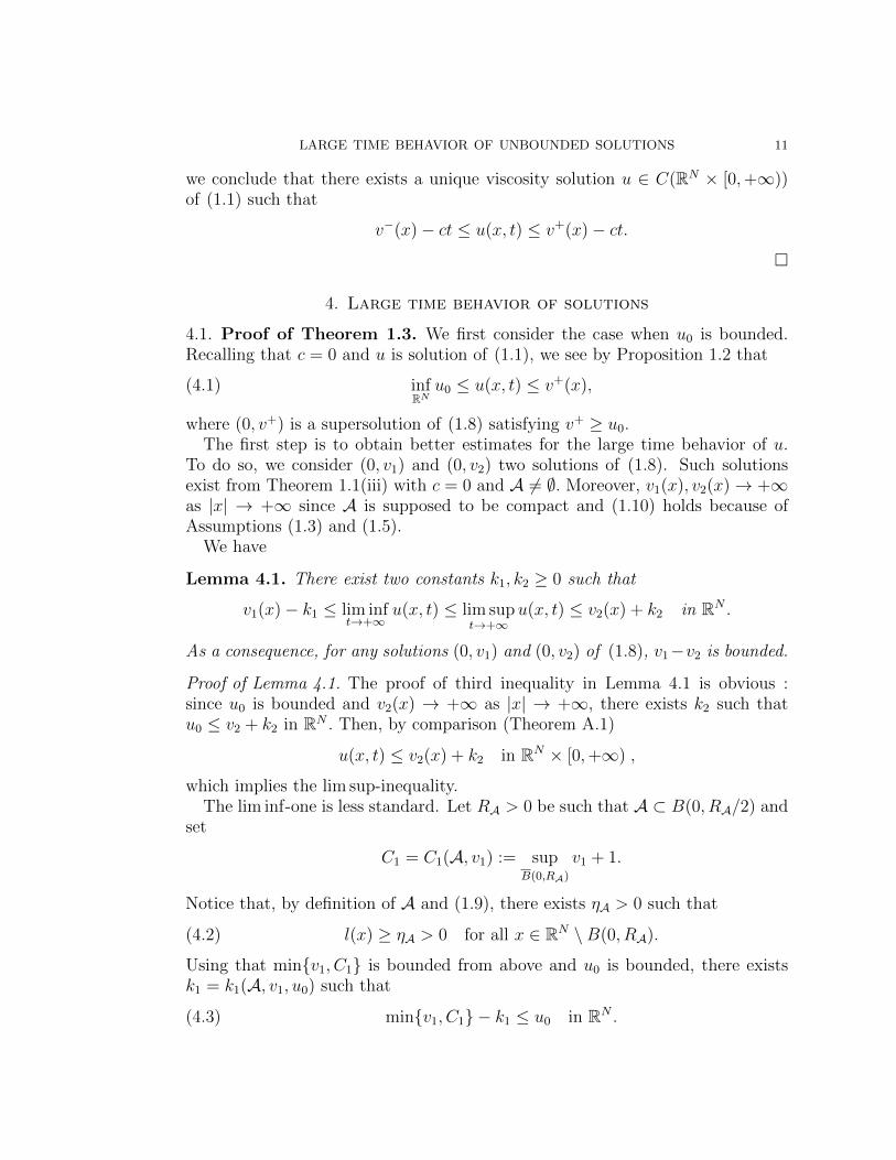
Lemma 4.1. There exist two constants k1, k2 ≥ 0 such that

v1(x)− k1 ≤ lim inft→+∞

u(x, t) ≤ lim supt→+∞

u(x, t) ≤ v2(x) + k2 in RN .

As a consequence, for any solutions (0, v1) and (0, v2) of (1.8), v1−v2 is bounded.

Proof of Lemma 4.1. The proof of third inequality in Lemma 4.1 is obvious :since u0 is bounded and v2(x) → +∞ as |x| → +∞, there exists k2 such thatu0 ≤ v2 + k2 in RN . Then, by comparison (Theorem A.1)

u(x, t) ≤ v2(x) + k2 in RN × [0,+∞) ,

which implies the lim sup-inequality.The lim inf-one is less standard. Let RA > 0 be such that A ⊂ B(0, RA/2) and

set

C1 = C1(A, v1) := supB(0,RA)

v1 + 1.

Notice that, by definition of A and (1.9), there exists ηA > 0 such that

l(x) ≥ ηA > 0 for all x ∈ RN \B(0, RA).(4.2)

Using that minv1, C1 is bounded from above and u0 is bounded, there existsk1 = k1(A, v1, u0) such that

minv1, C1 − k1 ≤ u0 in RN .(4.3)


Next we have to examine the large time behavior of the solution associated tothe initial condition minv1, C1− k1 and to do so, we use the following result ofBarron and Jensen (see Appendix).

Lemma 4.2. [8] Assume (1.4) and let u, u be locally Lipschitz subsolutions (resp.solutions) of (1.1). Then minu, u is still a subsolution (resp. a solution)of (1.1).

To use it, we remark that the function w−(x, t) := C1 + ηAt is a smoothsubsolution of (1.1) in (RN \B(0, RA))× (0,+∞). Indeed, for all |x| > RA, t > 0,

w−t +H(x,Dw−) = ηA +H(x, 0) = ηA ≤ l(x)

using (1.3) and (4.2). Since v1 is a locally Lipschitz continuous subsolution of (1.1)in RN×(0,+∞), we can use Lemma 4.2 in (RN \B(0, RA))×(0,+∞) to concludethat minv1, w

− − k1 is a subsolution, while in a neighborhood of B(0, RA) ×(0,+∞), we have minv1, w

− − k1 = v1 − k1 by definition of C1.Then, by comparison (Theorem A.1)

minv1(x), C1 + ηAt − k1 ≤ u(x, t) in RN × [0,+∞) ,

and one concludes easily.The last assertion of Lemma 4.1 is obvious since v1, v2 are arbitrary solutions

of (1.8) and we can exchange their roles.

The next step of the proof of Theorem 1.3 consists in introducing the half-relaxed limits [9, 3]

u(x) = lim inf∗t→+∞

u(x, t), u(x) = lim sup∗t→+∞

u(x, t).

They are well-defined for all x ∈ RN thanks to (4.1) or Lemma 4.1. We recall thatu ≤ u by definition and u = u if and only if u(x, t) converges locally uniformly inRN as t→ +∞. Therefore, to prove (1.12), it is enough to prove u ≤ u in RN .

A formal direct proof of this inequality is easy: u is a subsolution of (1.8), whileu is a supersolution of (1.8); by Lemma 4.2, for any constant C > 0, minu,Cis still a subsolution of (1.8) and Lemma 4.1 shows that minu,C − u → −∞as |x| → +∞. Moreover 0 is a strict subsolution of (1.8) outside A, therefore bycomparison arguments of Ishii [20]

maxRNminu,C − u ≤ max

Aminu,C − u ,

and letting C tend to +∞ gives u− u ≤ maxAu− u. But the right-hand sideis 0 since u(x, t) is decreasing in t on A using H(x, p) ≥ 0 and l(x) = 0 if x ∈ A.This gives the result.

This formal proof, although almost correct, is not correct since we do not havea local uniform convergence of u in a neighborhood of A, in particular because


we do not have equicontinuity of the family u(·, t), t ≥ 0. To overcome thisdifficulty, we use some approximations by inf- and sup-convolutions.

For all ε > 0, we introduce

uε(x, t) = infs∈(0,+∞)

u(x, s) +|t− s|2

ε2,

uε(x, t) = sups∈(0,+∞)

u(x, s)− |t− s|2

ε2.

By (4.1), they are well-defined for all (x, t) ∈ RN × [0,+∞) and we have

infRN

u0 ≤ uε(x, t) ≤ u(x, t) ≤ uε(x, t) ≤ v+(x).(4.4)

Notice that the infimum and the supremum are achieved in uε(x, t) and uε(x, t)respectively. Moreover Lemma 4.1 still holds for uε and uε. Taking in the sameway the half-relaxed limits for uε and uε, we obtain (with obvious notations)

infRN

u0 ≤ uε ≤ u ≤ u ≤ uε ≤ v+ in RN .

To prove the convergence result (1.12), it is therefore sufficient to establish

uε ≤ uε in RN ,(4.5)

which is our purpose from now on.

The following lemma, the proof of which is standard and left to the reader,collects some useful properties of uε and uε.

Lemma 4.3.(i) The functions uε and uε converge locally uniformly to u in RN × [0,+∞) asε→ 0.

(ii) The functions uε and uε are Lipschitz continuous with respect to t locallyuniformly in space, i.e., for all R > 0, there exists Cε,R > 0 such that, for allx ∈ B(0, R), t, t′ ≥ 0,

|uε(x, t)− uε(x, t′)|, |uε(x, t)− uε(x, t′)| ≤ Cε,R|t− t′|.(4.6)

(iii) For all open bounded subset Ω ⊂ RN , here exists tε,Ω > 0 with tε,Ω → 0as ε → 0, such that uε is solution of (1.1) and uε is subsolution of (1.1) inΩ× (tε,Ω,+∞).

(iv) For all R > 0, there exists Cε,R, tε,R > 0 such that, for all t > tε,R, uε(·, t)and uε(·, t) are subsolutions of

H(x,Dw(x)) ≤ l(x) + c+ 2Cε,R, in B(0, R).(4.7)

Therefore, uε(·, t) and uε(·, t) are locally Lipschitz continuous in space with aLipschitz constant independent of t.


We are now ready to prove that uε(·, t) and uε(·, t) converge uniformly on Aas t → +∞. We follow the arguments of [25] (or alternatively, one may use [10,Theorem I.14]). We fix R > 0 such that A ⊂ B(0, R) and consider tε,R > 0given by Lemma 4.3. Since w = uε or w = uε is a locally Lipschitz continuoussubsolution of (1.1) in B(0, R)× (tε,R,+∞), we have

wt(x, t) ≤ wt(x, t) +H(x,Dw(x, t)) ≤ l(x), a.e. (x, t),(4.8)

since H ≥ 0 by (1.3). Let x ∈ A, t > tε,R, and h, r > 0. We have

1

|B(x, r)|

∫B(x,r)

(w(y, t+ h)− w(y, t))dy

=1

|B(x, r)|

∫B(x,r)

∫ t+h

t

wt(y, s)dsdy

≤ 1

|B(x, r)|

∫B(x,r)

∫ t+h

t

l(y)dsdy

Using the continuity of w, l and l(x) = 0, and letting r → 0, we obtain

w(x, t+ h) ≤ w(x, t) for all x ∈ A, t > tε,R, h ≥ 0.(4.9)

Therefore t 7→ w(x, t) is a nonincreasing function on [tε,R,∞), Lipschitz contin-uous in space on the compact subset A (uniformly in time) and bounded frombelow according to (4.4). By Dini Theorem, w(·, t) converges uniformly on Aas t → +∞ to a Lipschitz continuous function. Therefore, there exist Lipschitzcontinuous functions φε, φ

ε : A → R with φε ≤ φε and

uε(x, t)→ φε(x), uε(x, t)→ φε(x), uniformly on A as t→ +∞.

We now use the previous results to prove the convergence of u on A. ByLemma 4.3(i), we first obtain that (4.9) holds for u. Therefore t 7→ u(x, t) isnonincreasing for x ∈ A, so u(·, t) converges pointwise as t→ +∞ to some func-tion φ : A → R. Notice that we cannot conclude to the uniform convergence atthis step since we do not know that φ is continuous.

We claim that uε(x, t), uε(x, t)→ φ(x) as t→ +∞, for all x ∈ A. The proof is

similar in both cases so we only provide it for uε(x, t). Let x ∈ A and s > 0 besuch that

u(x, s) +|t− s|2

ε2= uε(x, t) ≤ u(x, t).(4.10)

By (4.4), we have

|t− s|2

ε2≤ v+(x)− inf u0.


It follows that s → +∞ as t → +∞. Thanks to the pointwise convergenceu(x, s)→ φ(x) as s→ +∞, sending t to +∞ in (4.10), we obtain

φ(x) + lim supt→+∞

|t− s|2

ε2≤ φ(x),

from which we infer limt→+∞|t−s|2ε2

= 0. Therefore, by (4.10), uε(x, t) → φ(x).The claim is proved, which implies φε = φε = φ on A.

At this stage, we can apply here the above formal argument to the locallyLipschitz continuous functions uε and uε, noticing that uε and uε are also locallyLipschitz continuous functions. We deduce that

maxRNminuε, C − uε ≤ max

Aminuε, C − uε = max

Aminφ,C − φ,

and therefore letting C tend to +∞ we have uε = uε in RN .

Recalling that uε ≤ u ≤ u ≤ uε in RN , we have also u = u in RN , and theconclusion follows, completing the proof of the case when u0 is bounded.

We consider now the case when u0 is only bounded from below (but not neces-sarely from above). We set uC0 = minu0, C. If w denotes the solution of (1.1)associated to the initial data 0, then, because of the Barron-Jensen results, thesolution associated to uC0 is minu,w + C.

But, from the first step, we know that (i) w converges locally uniformly to somesolution v1 of (1.8), (ii) minu,w + C converges to some solution vC2 of (1.8)(depending perhaps on C) and (iii) we have (4.1) for u.

Let K be any compact subset of RN . If C is large enough in order to havev1 + C > v+ on K (the size of such C depends only on K), then for large t,minu,w + C = u on K by the uniform convergence of w to v1 on K. It followsthat u converges locally uniformly to vC2 on K, which is independent on C. Theproof of Theorem 1.3 is complete.

To conclude this section, we point out the following result which is a conse-quence of the comparison argument we used in the proof.

Corollary 4.4. Assume (1.2)-(1.3)-(1.4)-(1.5), l ≥ 0 and (1.9). Then, for allbounded from below solutions (0, v1) and (0, v2) of (1.8), v1, v2 → +∞ as |x| →+∞ and

supRN

v1 − v2 ≤ maxAv1 − v2 < +∞.

Remark 4.5. It is quite surprising that, though a lot of different solutions to (1.8)may exist (see Section 5.1), all the bounded from below solutions associated toc = −min l have the same growth at infinity. This is not true when A is notcompact, e.g., in the periodic case. Consider for instance

|Dv| = |sin(x)| in R.


For c = −minR |sin(x)| = 0, it is possible to build infinitely many solutions withvery different behaviors by gluing some branches of cosine functions, see Figure 1.

Figure 1. Some solutions of |Dv| = |sin(x)| in R, A = πZ

4.2. Proof of Theorem 1.4. By (1.13), there exists a subsolution (0, ψ) of (1.8)such that, for every ε > 0, there exists Rε > 0 such that, for all |x| ≥ Rε,

minψ(x), v(x) − ε ≤ minψ(x), u0(x) ≤ minψ(x), v(x)+ ε.(4.11)

Let Mε > 0 be such that

−Mε ≤ u0(x), v(x) for all |x| ≤ Rε.

Setting ψε(x) = minψ(x),−Mε, we claim that, for all x ∈ RN ,

minψε(x), v(x) − ε ≤ minψε(x), u0(x) ≤ minψε(x), v(x)+ ε.(4.12)

Indeed, this inequality comes from the M -property (4.11) if |x| ≥ Rε, while it isobvious by the choice of Mε, if |x| ≤ Rε.

From Lemma 4.2, (0, ψε) is a subsolution of (1.8) as a minimum of subsolu-tions. Since c ≥ 0, (c, ψε) is also subsolution of (1.8). Applying again Lemma 4.2to (c, ψε) and (c, v), we obtain that (c,minψε, v) is a subsolution of (1.8).From (4.12), we have minψε, v − ε ≤ u0. It follows from Proposition 1.2,that there exists a unique viscosity solution u of (1.1) with initial data u0 and itsatisfies

minψε, v − ε ≤ u(x, t) + ct ≤ v+(x),(4.13)

where (c, v+) is a supersolution of (1.8) such that u0 ≤ v+.In the same way, there exists unique viscosity solutions wε and w of (1.1) asso-

ciated with initial datas ψε and 0 respectively. Since ψε ≤ −Mε, by comparisonand Proposition 1.2, we have

ψε(x) ≤ wε(x, t) ≤ −Mε + w(x, t) ≤ v+(x) for (x, t) ∈ RN × [0,+∞),(4.14)

where (0, v+) is a supersolution of (1.8) such that −Mε ≤ v+.


Arguing as at the end of the proof of Theorem 1.3, the solutions of (1.1)associated to the initial datas

minψε(x), v(x) − ε, minψε(x), u0(x) and minψε(x), v(x)+ ε

are respectively

minwε(x, t), v(x)−ct−ε, minwε(x, t), u(x, t) and minwε(x, t), v(x)−ct+ε.

By comparison, we have, in RN × (0,+∞)

minwε(x, t), v(x)− ct − ε ≤ minwε(x, t), u(x, t) ,

and

minwε(x, t), u(x, t) ≤ minwε(x, t), v(x)− ct+ ε.

Recalling that c is positive and using (4.14), if K is a compact subset of RN , thenfor t large enough and x ∈ K

minwε(x, t), v(x)− ct = v(x)− ct ,

leading to the inequality

v(x)− ct− ε ≤ minwε(x, t), u(x, t) ≤ v(x)− ct+ ε.

From (4.13) and (4.14), t can be chosen large enough to have wε(x, t) + ct >u(x, t) + ct so we end up with

v(x)− ct− ε ≤ u(x, t) ≤ v(x)− ct+ ε,

for t large enough and x in K. Since ε is arbitrary, the conclusion follows.

Remark 4.6. Theorem 1.4 is very close to [18, Theorem 5.3]. In the latter paper,the authors obtain the convergence assuming that infRNu0−minψ, v > −∞and

limr→+∞

|(u0 − v)(x)| : ψ(x) > v(x) + r = 0.(4.15)

We do not know if this assumption is equivalent to ours. But in both assumptions,the point is that u0(x) must be close to v(x) when v(x) is “far below” ψ(x), whichmeans ψ(x) > v(x) + r for large r in (4.15) and minψ(x),−r > v(x) for large rin our case. This situation occurs for instance if v, u0 are unbounded from belowand close when v(x)→ −∞.

5. Optimal control problem and examples

Consider the one-dimensional Hamilton-Jacobi Equationut(x, t) + |Du(x, t)| = 1 + |x| in R× (0,∞)

u(x, 0) = u0(x),(5.1)


where l(x) = |x|+1 ≥ 0, minRN l = 1, and A = argmin l = 0 satisfies (1.9). Wecan come back to our framework by looking at u(x, t) = u(x, t)− t which solves

ut(x, t) + |Du(x, t)| = |x| in R× (0,∞) ,

where l(x) := |x| satisfies the assumptions of our results.There exists a unique continuous solution u of (5.1) for every continuous u0

satisfying |u0(x)| ≤ C(1 + |x|2) (use Theorem A.1 and the fact that ±KeKt(1 +|x|2) are super- and subsolution for large K).

We can represent u as the value function of the following associated deter-ministic optimal control problem. Consider the controlled ordinary differentialequation

X(s) = α(s),

X(0) = x ∈ R,(5.2)

where the control α(·) ∈ L∞([0,+∞); [−1, 1]) (i.e., |α(t)| ≤ 1 a.e. t ≥ 0). For

any given control α, (5.2) has a unique solution X(t) = Xx,α(·) = x +∫ t

0α(s)ds.

We define the cost functional

J(x, t, α) =

∫ t

0

(|X(s)|+ 1)ds+ u0(X(t)),

and the value function

V (x, t) = infα∈L∞([0,+∞);[−1,1])

J(x, t, α).

It is classical to check that V (x, t) = u(x, t) is the unique viscosity solutionof (5.1), see [3, 2].

5.1. Solutions to the ergodic problem. There are infinitely many essentiallydifferent solutions with different constants to the associated ergodic problem

|Dv(x)| = 1 + |x|+ c in R.(5.3)

Define S(x) =∫ x

0|y|dy. The following pairs (c, v) are solutions.

• (−1, 12x2) and (−1,−1

2x2). They are bounded from below (respectively

from above) with c = −min l;• (−1, S(x)) and (−1,−S(x)). They are neither bounded from below nor

from above and c = −min l;• (λ − 1, λx + S(x)) and (λ − 1,−λx − S(x)) for every λ > 0. They are

neither bounded from below nor from above and c > −min l;• (λ − 1,−1

2x2 − λ|x|) for every λ > 0. These solutions are nonsmooth

(notice that −v is not anymore a viscosity solution), they are not boundedfrom below. Actually, they are the solutions obtained by the constructiveproof of Theorem 1.1(i). Indeed, the unique solution VR of the Dirichlet


problem (2.3) is VR(x) = R2−x22

+ λ(R − |x|) for x ∈ [−R,R], leading to

v(x) = limR→∞VR(x)− VR(0) = −12x2 − λ|x|.

• (c, v) where (c, v1) and (c, v2) are solutions, v = minv1 +C1, v2 +C2 andC1, C2 ∈ R. This is a consequence of Lemma 4.2.

5.2. Equation (5.1) with u0(x) = S(x). For any solution (c, v) to (5.3), it isobvious that u(x, t) = −ct+v(x) is the unique solution to (5.1) with u0(x) = v(x)and the convergence holds, i.e., u(x, t) + ct → v(x) as t → +∞. In particular, ifu0(x) = S(x), the solution of (5.1) is u(x, t) = t+ S(x).

Let us find in another way the solution by computing the value function of thecontrol problem stated above. Let t > 0. We compute V (x, t) for any x ∈ R bydetermining the optimal controls and trajectories.

1st case: x ≥ 0.There are infinitely many optimal strategies: they consist in going as quickly aspossible to 0 (= argmin l), to wait at 0 for a while and to go as quickly as possibletowards −∞. For any 0 ≤ τ ≤ t− x, it corresponds to the optimal controls andtrajectories

α(s) =

−1, 0 ≤ s ≤ x,0, x ≤ s ≤ x+ τ,−1, x+ τ ≤ s ≤ t,

X(s) =

x− s, 0 ≤ s ≤ x,0, x ≤ s ≤ x+ τ,

−(s− x− τ), x+ τ ≤ s ≤ t.(5.4)

They lead to V (x, t) = J(x, t, α) = t + S(x). Among these optimal strategies,there are two of particular interest:

• The first one is to go as quickly as possible to 0 and to remain there(τ = t−x). This strategy is typical of what happens in the periodic case:the optimal trajectories are attracted by A = argmin l.• The second one is to go as quickly as possible towards −∞ during all the

available time t (τ = 0). This situation is very different to the periodiccase. Due to the unbounded (from below) final cost u0, some optimaltrajectories are not anymore atttracted by argmin l and are unbounded.

2nd case: x < 0.In this case there is not anymore bounded optimal trajectories. The only optimalstrategy is to go as quickly as possible towards −∞. The optimal control areα(s) = −1, X(s) = x−s for 0 ≤ s ≤ t leading to V (x, t) = J(x, t,−1) = t+S(x).

The analysis of this case in terms of control will help us for the followingexamples.

5.3. Equation (5.1) with u0(x) = 12x2 + b(x) with b bounded from below.

To illustrate Theorem 1.3, we choose an initial condition which is a bounded per-turbation of a bounded from below solution of the ergodic problem. To simplifythe computations, we choose a periodic perturbation b.


For any x, an optimal strategy can be chosen among those described in Exam-ple 5.2. More precisely: go as quickly as possible to 0, wait nearly until time tand move a little to reach the minimum of the periodic perturbation. For t largeenough (at least t > x), we compute the cost with α,X given by (5.4),

J(x, t, α) = t+1

2x2 + b(−t+ x+ τ).

For every t large enough, there exists 0 ≤ τ = τt < t−x such that b(−t+x+τt) =min b. It leads to

V (x, t) = J(x, t, α) = t+1

2x2 + min b.

Therefore, we have the convergence as announced in Theorem 1.3.

5.4. Equation (5.1) with u0(x) = S(x) + b(x) with b bounded Lipschitzcontinuous. We compute the value function as above. Due to the unbounded-ness from below of u0 we need to distinguish the cases x ≥ 0 and x < 0 as inExample 5.2.

1st case: x ≥ 0.We use the same strategy as in Example 5.3 leading to V (x, t) = J(x, t, α) =t+ 1

2x2 + min b.

2nd case: x < 0.In this case, the optimal strategy suggested by Examples 5.2 and 5.3 is to startby waiting a small time τ before going as quickly as possible towards −∞. Thewaiting time correspond to an attempt to reach a minimum of b at the left endof the trajectory. It corresponds to the control and trajectory

α(s) =

0, 0 ≤ s ≤ τ,−1, τ ≤ s ≤ t,

X(s) =

x, 0 ≤ s ≤ τ,x− (s− τ), τ ≤ s ≤ t,

leading to

J(x, t, α) = t+ S(x) + τ |x|+ b(x− t+ τ).

Due to the boundedness of b, in order to be optimal, we see that necessarilyτ = O(1/|x|) to keep bounded the positive term τ |x| in J(x, t, α). So, for large|x|, x < 0, we have b(x− t+ τ) ≈ b(x− t). When b is not constant, b(x− t) hasno limit as t→ +∞, the convergence for V (x, t) cannot hold.

In this case, u0 is a bounded perturbation of a solution (c, v) = (−1, S(x)) ofthe ergodic problem with c = −min l but v is not bounded from below and theconvergence of the value function may not hold. It follows that the assumptionsof Theorem 1.3 cannot be weakened easily. In particular, the boundedness frombelow of the solution of the ergodic problem seems to be crucial.


5.5. Equation (5.1) with u0(x) = S(x) + x + sin(x). The solution of (5.1) isu(x, t) = S(x)+x+sin(x−t). Clearly, we do not have the convergence. In this case,u0 is a bounded perturbation of the solution (0, S(x) + x) of the ergodic problemwith c > −min l and S(x)+x−u0(x) 6→ 0 as x→ −∞ (where S(x)+x→ −∞).This example shows that the convergence in Theorem 1.4 may fail when (1.13)does not hold.

Appendix A. Comparison principle for the solutions of (1.1)

The comparison result for the unbounded solutions of (1.1) is a consequenceof a general comparison result for first-order Hamilton-Jacobi equations whichholds without growth conditions at infinity.

Theorem A.1. [19, 23] Assume that H satisfies (1.5) and that u ∈ USC(RN ×[0, T ]) and v ∈ LSC(RN×[0, T ]) are respectively a subsolution of (1.1) with initialdata u0 ∈ C(RN) and a supersolution of (1.1) with initial data v0 ∈ C(RN). Then,for every x0 ∈ RN and r > 0,

u(x, t)− v(x, t) ≤ supB(x0,r)

u0(y)− v0(y) for every (x, t) ∈ D(x0, r),

where

D(x0, r) = (x, t) ∈ B(x0, r)× (0, T ) : eCHT (1 + |x− x0|)− 1 ≤ r.

When supRNu0 − v0 < +∞, a straightforward consequence is

u(x, t)− v(x, t) ≤ supRN

u0 − v0 for every (x, t) ∈ RN × [0,+∞).

Appendix B. Barron-Jensen solutions of convex HJ equations

Theorem B.1. Assume that H satisfies (1.4) and (1.5). Then u ∈ W 1,∞loc (RN ×

(0,+∞)) is a viscosity solution (respectively subsolution) of (1.1) if and ony ifit is a Barron-Jensen solution (respectively subsolution) of (1.1), i.e., for every(x, t) ∈ RN × (0,+∞) and ϕ ∈ C1(RN × (0,+∞)) such that u − ϕ has a localminimum at (x, t), one has

ϕt(x, t) +H(x,Dϕ(x, t)) = l(x) (respectively ≤ l(x)).

This result is due to Barron and Jensen [8] and we refer to Barles [1, p. 89].Lemmas 4.3(iii) and 4.2 are consequences of this theorem.

As far as Lemma 4.3(iii) is concerned, the fact that the inf-convolution (respec-tively the sup-convolution) preserves the supersolution (respectively the subsolu-tion) property is classical ([3, 2]). What is more suprising is the preservation ofthe subsolution property of the inf-convolution which comes from the convexityof H and the Theorem of Barron-Jensen B.1. For a proof, notice first that U ,being a solution of (1.1), is a Barron-Jensen solution of (1.1). We then apply [23,Lemma 3.2] using that H, l are independent of t.


For Lemma 4.2, we refer the reader to [1, Theorem 9.2, p.90].

References

[1] Yves Achdou, Guy Barles, Hitoshi Ishii, and Grigory L. Litvinov. Hamilton-Jacobi equa-tions: approximations, numerical analysis and applications, volume 2074 of Lecture Notesin Mathematics. Springer, Heidelberg; Fondazione C.I.M.E., Florence, 2013. Lecture Notesfrom the CIME Summer School held in Cetraro, August 29–September 3, 2011, Edited byPaola Loreti and Nicoletta Anna Tchou, Fondazione CIME/CIME Foundation Subseries.

[2] M. Bardi and I. Capuzzo Dolcetta. Optimal control and viscosity solutions of Hamilton-Jacobi-Bellman equations. Birkhauser Boston Inc., Boston, MA, 1997.

[3] G. Barles. Solutions de viscosite des equations de Hamilton-Jacobi. Springer-Verlag, Paris,1994.

[4] G. Barles and J.-M. Roquejoffre. Ergodic type problems and large time behaviour of un-bounded solutions of Hamilton-Jacobi equations. Comm. Partial Differential Equations,31(7-9):1209–1225, 2006.

[5] G. Barles and P. E. Souganidis. On the large time behavior of solutions of Hamilton-Jacobiequations. SIAM J. Math. Anal., 31(4):925–939 (electronic), 2000.

[6] Guy Barles, Hitoshi Ishii, and Hiroyoshi Mitake. A new PDE approach to the large timeasymptotics of solutions of Hamilton-Jacobi equations. Bull. Math. Sci., 3(3):363–388,2013.

[7] Guy Barles and Joao Meireles. On unbounded solutions of ergodic problems in Rm forviscous Hamilton-Jacobi equations. Comm. Partial Differential Equations, 41(12):1985–2003, 2016.

[8] E. N. Barron and R. Jensen. Semicontinuous viscosity solutions of Hamilton-Jacobi equa-tions with convex hamiltonians. Comm. Partial Differential Equations, 15(12):1713–1740,1990.

[9] M. G. Crandall, H. Ishii, and P.-L. Lions. User’s guide to viscosity solutions of second orderpartial differential equations. Bull. Amer. Math. Soc. (N.S.), 27(1):1–67, 1992.

[10] M. G. Crandall and P.-L. Lions. Viscosity solutions of Hamilton-Jacobi equations. Trans.Amer. Math. Soc., 277(1):1–42, 1983.

[11] F. Da Lio. Comparison results for quasilinear equations in annular domains and applica-tions. Comm. Partial Differential Equations, 27(1-2):283–323, 2002.

[12] A. Davini and A. Siconolfi. A generalized dynamical approach to the large time behavior ofsolutions of Hamilton-Jacobi equations. SIAM J. Math. Anal., 38(2):478–502 (electronic),2006.

[13] A. Fathi. Sur la convergence du semi-groupe de Lax-Oleinik. C. R. Acad. Sci. Paris Ser.I Math., 327(3):267–270, 1998.

[14] A. Fathi and A. Siconolfi. Existence of C1 critical subsolutions of the Hamilton-Jacobiequation. Invent. Math., 155(2):363–388, 2004.

[15] A. Fathi and A. Siconolfi. PDE aspects of Aubry-Mather theory for quasiconvex Hamilto-nians. Calc. Var. Partial Differential Equations, 22(2):185–228, 2005.

[16] Albert Fathi and Ezequiel Maderna. Weak KAM theorem on non compact manifolds.NoDEA Nonlinear Differential Equations Appl., 14(1-2):1–27, 2007.

[17] Naoyuki Ichihara and Hitoshi Ishii. The large-time behavior of solutions of Hamilton-Jacobiequations on the real line. Methods Appl. Anal., 15(2):223–242, 2008.

[18] Naoyuki Ichihara and Hitoshi Ishii. Long-time behavior of solutions of Hamilton-Jacobiequations with convex and coercive Hamiltonians. Arch. Ration. Mech. Anal., 194(2):383–419, 2009.


[19] H. Ishii. Uniqueness of unbounded viscosity solution of Hamilton-Jacobi equations. IndianaUniv. Math. J., 33(5):721–748, 1984.

[20] H. Ishii. A simple, direct proof of uniqueness for solutions of the Hamilton-Jacobi equationsof eikonal type. Proc. Amer. Math. Soc., 100(2):247–251, 1987.

[21] H. Ishii. Asymptotic solutions for large time of Hamilton-Jacobi equations in Euclidean nspace. Ann. Inst. H. Poincare Anal. Non Lineaire, 25(2):231–266, 2008.

[22] H. Ishii. Asymptotic solutions of Hamilton-Jacobi equations for large time and relatedtopics. In ICIAM 07—6th International Congress on Industrial and Applied Mathematics,pages 193–217. Eur. Math. Soc., Zurich, 2009.

[23] O. Ley. Lower-bound gradient estimates for first-order Hamilton-Jacobi equations andapplications to the regularity of propagating fronts. Adv. Differential Equations, 6(5):547–576, 2001.

[24] P.-L. Lions, B. Papanicolaou, and S. R. S. Varadhan. Homogenization of Hamilton-Jacobiequations. Unpublished, 1986.

[25] G. Namah and J.-M. Roquejoffre. Remarks on the long time behaviour of the solutions ofHamilton-Jacobi equations. Comm. Partial Differential Equations, 24(5-6):883–893, 1999.

LMPT, Federation Denis Poisson, Universite Francois-Rabelais Tours, FranceE-mail address: [email protected]

IRMAR, INSA Rennes, FranceE-mail address: [email protected]

Dipartimento di Matematica, Universita di Padova, ItalyE-mail address: [email protected]

Faculty of Mathematics and Statistics, Ton Duc Thang University, Ho ChiMinh City, Vietnam

E-mail address: [email protected]

Documents

Guy Barles, Olivier Ley, Thi-Tuyen Nguyen, Thanh Phan