Embed Size (px)
Citation preview
Bureau International des Poids et Mesures
Guide to
the Realization of the ITS-90
Platinum Resistance Thermometry
Consultative Committee for Thermometry
under the auspices of the
International Committee for Weights and Measures
Guide to the Realization of the ITS-90
Platinum Resistance Thermometry
2 / 56
Platinum Resistance Thermometry
CONTENTS
1 Introduction
2 The SPRT definitions in ITS-90
2.1 Overview of the scale definition
2.2 Reference functions
2.3 Interpolating equations
2.3.1 Interpolating equations prescribed in the ITS-90 text
2.3.2 Alternative interpolating equations for special applications
2.4 Continuity of ITS-90
3 Design and operation of SPRTs
3.1 Operating principles and overview
3.2 Typical designs of SPRTs
3.2.1 Capsule-type standard platinum resistance thermometer
3.2.2 Long-stem standard platinum resistance thermometer
3.2.3 High-temperature standard platinum resistance thermometer
4 Standard platinum resistance thermometer use and care
4.1 Mechanical treatment and shipping precautions
4.2 Thermal treatment and annealing
4.3 Devitrification
4.4 Calibration
4.4.1 Calibration procedures
4.4.2 Consistency checks
4.4.3 Reporting
5 Experimental sources of uncertainty
5.1 Factors affecting SPRT resistance
5.1.1 Oxidation
5.1.2 Impurities
5.1.3 Strain and hysteresis
5.1.4 Vacancies and defects
5.1.5 Moisture
Guide to the Realization of the ITS-90 Platinum Resistance Thermometry
3 / 56
5.1.6 High-temperature insulation breakdown and contamination
5.2 Thermal effects arising in use
5.2.1 Conduction and immersion effects
5.2.2 Radiation effects
5.3 Resistance measurement
5.3.1 Resistance bridges
5.3.2 Reference resistor
5.3.3 Self heating
5.3.4 Connecting cables and lead resistances
6 Uncertainty in SPRT calibrations
6.1 Uncertainty of SPRT calibration at the fixed points
6.1.1 Uncertainty in SPRT resistance at the triple point of water
6.1.2 Uncertainty in SPRT resistance ratios at fixed points
6.2 Propagation of calibration uncertainty
6.2.1 Fixed-point sensitivity coefficients and propagation equation without
correlations
6.2.2 Propagated uncertainty
6.3 Non-uniqueness due to interpolation errors
6.3.1 Type 1 non-uniqueness (sub-range inconsistency)
6.3.2 Type 3 non-uniqueness
6.4 Total uncertainty in realised temperature
References
Appendix 1: Alternative interpolating functions for special applications
Appendix 2: Typical resistance ratios and sensitivity factors for SPRTs in the ITS-90, as well
as the propagation of uncertainty from the triple point of water
Appendix 3: Summary of typical ranges of Type B standard uncertainties of the calibration of
SPRTs at the fixed points
Last updated 1 January 2018
Guide to the Realization of the ITS-90
Platinum Resistance Thermometry
4 / 56
Guide to the Realization of the ITS-90
Platinum Resistance Thermometry
A I Pokhodun, D I Mendeleyev Institute for Metrology, Russia
B Fellmuth, Physikalisch-Technische Bundesanstalt, Berlin, Germany
J V Pearce, National Physical Laboratory, Teddington, United Kingdom
R L Rusby, National Physical Laboratory, Teddington, United Kingdom
P P M Steur, Istituto Nazionale di Ricerca Metrologica, Torino, Italy
O Tamura, National Metrology Institute of Japan, AIST, Tsukuba, Japan
W L Tew, National Institute of Standards and Technology, Gaithersburg, USA
D R White, Measurement Standards Laboratory of New Zealand, Lower Hutt, New Zealand
Abstract
This paper is a part of guidelines, prepared on behalf of the Consultative Committee for Thermometry,
on the methods how to realize the International Temperature Scale of 1990.
It discusses the major issues linked to platinum resistance thermometry for the realization of the
International Temperature Scale of 1990 in the temperature range from 24.5561 K to 1234.93 K.
Guide to the Realization of the ITS-90 Platinum Resistance Thermometry
5 / 56
1 INTRODUCTION
In the temperature range from the triple point of equilibrium hydrogen (13.8033 K) to the freezing
point of silver (1234.93 K), the ITS-90 is defined in terms of the temperature dependence of the
electrical resistance of standard platinum resistance thermometers (SPRTs). This chapter provides
mainly an overview of the practical realisation of the scale in the restricted range from the triple point
of neon (24.5561 K) to the freezing point of silver, which does not require to realise the vapour-pressure
points of equilibrium hydrogen in the vicinity of 17 K and 20.3 K or to apply an interpolating helium
constant-volume gas thermometer. Furthermore, it includes an explanation of the scale definition,
describes the different types of SPRTs used, gives advice on the use and calibration of SPRTs, and
concludes with a brief summary of the sources of uncertainty. The chapter omits discussion of the fixed
points used to calibrate SPRTs, as this is covered in Chapter 2 Fixed Points
(http://www.bipm.org/en/committees/cc/cct/guide-its90.html) as well as in [Mangum et al. 1999 and
2000]. For more detail, the reader is referred to the references given at the end of the chapter and the
Technical Annex of the mise en pratique of the definition of the kelvin (MeP-K) [Ripple et al. 2010,
Fellmuth et al. 2016, http://www.bipm.org/en/publications/mep_kelvin/], which includes supplement-
ary definitions and clarifications.
2 THE SPRT DEFINITIONS IN ITS-90
2.1 Overview of the scale definition
The ITS-90 specifies a set of fixed points (melting, freezing, triple, or boiling points of various pure
substances, see Guide Chapter 2 Fixed points), which are used for the calibration of SPRTs in eleven
temperature sub-ranges within the overall range from 13.8033 K to 1234.93 K. All the sub-ranges
include the triple point of water (TPW) and extend to progressively higher or lower temperatures. The
existence of overlapping sub-ranges implies the existence of a variety of temperature values T90
according to the ITS-90 for a given resistance value for a given SPRT (Type 1 non-uniqueness (sub-
range inconsistency) [Mangum et al. 1997]), see Subsection 6.3.1. Mathematical procedures are
specified for relating the measured resistances of the SPRTs to the corresponding ITS-90 temperatures.
SPRT resistances are not used directly but are first normalised by taking ratios to the resistance at
the TPW (273.16 K). Thus, the ITS-90 resistance ratio, W(T90), is defined as
W(T90) = R(T90) / R(273.16 K) , (1)
where R(T90) and R(273.16 K) are the resistances of the SPRT at the temperature T90 and at the TPW,
respectively. Taking resistance ratios removes the need for traceability to absolute resistance standards
in the calibration and use of an SPRT. The W values embody that SPRT characteristics are
fundamentally similar, which allows the application of reference functions. Furthermore, the
normalisation provides some compensation for instability, though this is not something the ITS-90
considers. The compensation is perfect for temperature-independent relative resistance changes caused
for instance by dimensional changes in the platinum wire or by oxidation discussed in Subsection 5.1.1.
SPRTs must be made with strain-free wires of high purity platinum, so that the ratio W(T90), which
is essentially the ratio of the corresponding resistivities of the platinum wire, is very similar for all
SPRTs. This is needed so that different SPRTs have similar interpolation properties; that is, they
Guide to the Realization of the ITS-90
Platinum Resistance Thermometry
6 / 56
generate very similar realisations of the ITS-90. The purer and more strain-free the wire is, the higher
is the temperature coefficient of resistance. Therefore, to ensure the suitability of an SPRT, the ITS-90
specifies criteria for the temperature coefficient, based on the resistance ratios at the melting point of
gallium and at the triple point of mercury. The criteria are:
W(29.7646 °С) ≥ 1.118 07 (2)
and
W(−38.8344 °С) ≤ 0.844 235 . (3)
These criteria are approximately equivalent and are used in sub-ranges above or below 273.16 K. They
place lower limits on the temperature coefficient of the resistance of the platinum, and implicitly define
the minimum purity requirements for the wire used in SPRTs.
In order to limit the effect of a possible breakdown of electrical insulation within High-
Temperature SPRTs (HTSPRTs), the ITS-90 specifies an additional requirement for the resistance ratio
at the freezing point of silver:
W(961.78 °С) ≥ 4.2844 . (4)
Qualification criteria are discussed further in Subsection 4.4.2.
To interpolate between the values of W(T90) measured at a limited number of fixed points, the ITS-
90 defines two reference functions (one above and one below the TPW), which relate the resistance
ratio Wr(T90) of two chosen high-quality reference SPRTs, having high temperature coefficients of
resistance, to T90, see Subsection 2.2. The reference functions are continuous in their first and second
derivatives throughout the whole range 13.8033 K to 1234.93 K.
The interpolation is done by comparing the values of W(T90) at fixed points with the corresponding
values of Wr(T90) specified in the scale (Table 1 in the ITS-90 text). The differences (deviations) ΔW =
W(T90) - Wr(T90) are mapped by low-order functions (mostly simple polynomials in (W – 1) and/or
ln(W), see Subsection 2.3.1), which then allow differences to be interpolated at any point in the sub-
range. In each sub-range, different fixed points and interpolating equations are applied. For SPRTs
using high-purity strain-free platinum, it follows that the W(T90) functions are very similar, and
therefore that the deviations from the reference functions, Wr(T90), are small. The deviation functions
include the coefficients which are specific to the particular SPRT and whose values are determined
from the calibration data ΔW at the required fixed points.
Thus, the calibration of a particular SPRT has two components: the (relatively complicated)
reference function, Wr(T90), which is the same for all SPRTs, and the (relatively simple) deviation
function, ΔW, which contains the limited number of SPRT calibration coefficients derived from the
fixed-point measurements.
As an example of a deviation equation, in the sub-range from the TPW to the freezing point of
aluminium the specified equation is (omitting the qualifier T90)
∆W ≡ (W – Wr) = a (W – 1) + b (W – 1)2 + c (W – 1)3 . (5)
The values of the coefficients a, b, and c in Equation (5) are determined by requiring the equation to
be satisfied at each of the defining fixed points for the sub-range, in this case the freezing points of tin,
zinc, and aluminium. Hence:
Guide to the Realization of the ITS-90 Platinum Resistance Thermometry
7 / 56
2 3Sn r,Sn Sn Sn Sn
2 3Zn r,Zn Zn Zn Zn
2 3Al r,Al Al Al Al
( 1) ( 1) ( 1) ,
( 1) ( 1) ( 1) ,
( 1) ( 1) ( 1) ,
W W a W b W c W
W W a W b W c W
W W a W b W c W
− = − + − + −
− = − + − + −
− = − + − + −
(6a, 6b, 6c)
where WSn, WZn, and WAl are the measured values of resistance ratio at the indicated fixed points, and
Wr,Sn, Wr,Zn and Wr,Al are the values of reference resistance ratio assigned to the fixed points in the ITS-
90. Since there are three equations, the three unknowns, a, b, and c, are calculated exactly. The
Equation (5) can now be used to calculate the deviation (W - Wr), and hence Wr, for any input value of
W within the sub-range.
The same procedure is followed in other sub-ranges, but an additional term is specified for an
interpolation up to the silver point, and more complicated equations, involving terms in ln(W), are
required for the sub-ranges below the TPW, see Subsection 2.3.1. Additionally, the sub-range from the
triple point of mercury to the melting point of gallium extends above and below the TPW. Note that all
of the ITS-90 interpolating equations are formulated so that at the TPW Wr = 1, W = 1 and ΔW = 0.
Given the calibration coefficients for a particular SPRT in a particular sub-range, the calculation
of T90 from a measured resistance can be seen as a three-step mapping,
R(T90) → W(T90) → Wr(T90) → T90:
Step 1: Calculate the resistance ratio W(T90) = R(T90) / R(273.16 K),
Step 2: Use ∆W(W) and the coefficients to calculate ΔW, and hence Wr(T90) = W(T90) – ΔW,
Step 3: Use the reference function to calculate T90 from Wr(T90).
The first two steps are manipulations of the calibration data and interpolation involving W-values
only; it is not until the Step 3 that temperature appears as a variable. In Step 3, calculating T90 from the
reference function defining Wr(T90) requires iteration as it cannot be solved for T90 by direct substitution
of values of Wr. However, as an alternative the ITS-90 specifies inverse functions T90(Wr) which can
be used with good accuracy, see Subsection 2.2.
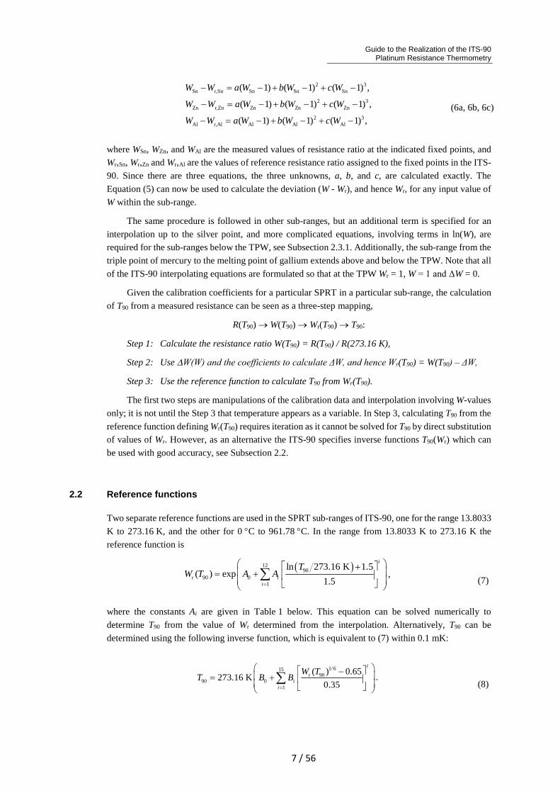
2.2 Reference functions
Two separate reference functions are used in the SPRT sub-ranges of ITS-90, one for the range 13.8033
K to 273.16 K, and the other for 0 °C to 961.78 °C. In the range from 13.8033 K to 273.16 K the
reference function is
( )1290
r 90 01
ln 273.16 K 1.5( ) exp
1.5
i
ii
TW T A A
=
+ = +
∑ , (7)
where the constants Ai are given in Table 1 below. This equation can be solved numerically to
determine T90 from the value of Wr determined from the interpolation. Alternatively, T90 can be
determined using the following inverse function, which is equivalent to (7) within 0.1 mK:
1/615r 90
90 01
( ) 0.65273.16 K
0.35
i
ii
W TT B B
=
− = +
∑ . (8)
Guide to the Realization of the ITS-90
Platinum Resistance Thermometry
8 / 56
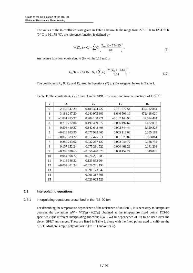
The values of the Bi coefficients are given in Table 1 below. In the range from 273.16 K to 1234.93 K
(0 °C to 961.78 °C), the reference function is defined by
990
r 90 01
K 754.15( )
481
i
ii
TW T C C
=
− = +
∑ .
(9)
An inverse function, equivalent to (9) within 0.13 mK is
9r 90
90 01
( ) 2.64K 273.15
1.64
i
ii
W TT D D
=
− = + +
∑ .
(10)
The coefficients Ai, Bi, Ci, and Di, used in Equations (7) to (10) are given below in Table 1.
Table 1: The constants Ai, Bi, Ci and Di in the SPRT reference and inverse functions of ITS-90.
i Ai Bi Ci Di
0 −2.135 347 29 0.183 324 722 2.781 572 54 439.932 854
1 3.183 247 20 0.240 975 303 1.646 509 16 472.418 020
2 −1.801 435 97 0.209 108 771 −0.137 143 90 37.684 494
3 0.717 272 04 0.190 439 972 −0.006 497 67 7.472 018
4 0.503 440 27 0.142 648 498 −0.002 344 44 2.920 828
5 −0.618 993 95 0.077 993 465 0.005 118 68 0.005 184
6 −0.053 323 22 0.012 475 611 0.001 879 82 −0.963 864
7 0.280 213 62 −0.032 267 127 −0.002 044 72 −0.188 732
8 0.107 152 24 −0.075 291 522 −0.000 461 22 0.191 203
9 −0.293 028 65 −0.056 470 670 0.000 457 24 0.049 025
10 0.044 598 72 0.076 201 285
11 0.118 686 32 0.123 893 204
12 −0.052 481 34 −0.029 201 193
13 −0.091 173 542
14 0.001 317 696
15 0.026 025 526
2.3 Interpolating equations
2.3.1 Interpolating equations prescribed in the ITS-90 text
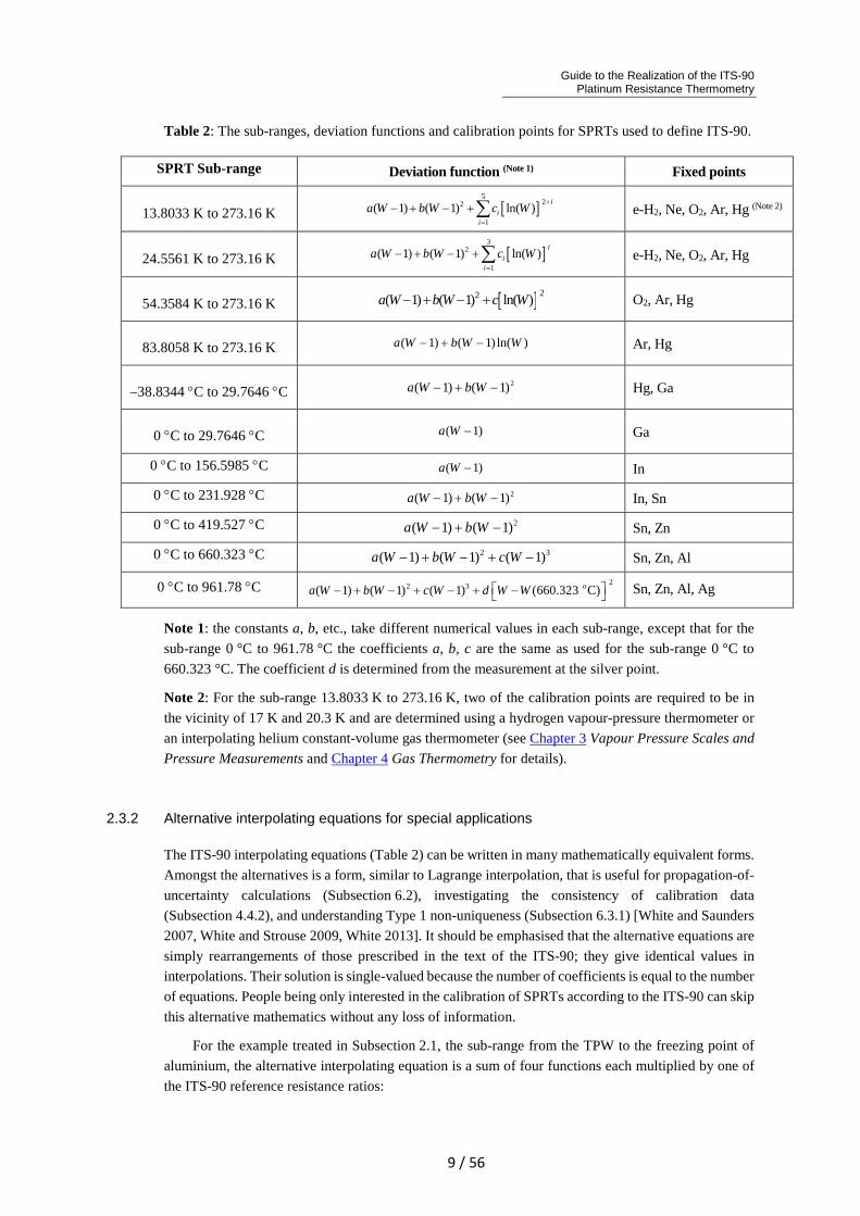
For describing the temperature dependence of the resistance of an SPRT, it is necessary to interpolate
between the deviations ΔW = W(T90) - Wr(T90) obtained at the temperature fixed points. ITS-90
specifies eight different interpolating functions ((W – Wr) in dependence of W) to be used over the
eleven SPRT sub-ranges. These are listed in Table 2, along with the fixed points used to calibrate the
SPRT. Most are simple polynomials in (W – 1) and/or ln(W).
Guide to the Realization of the ITS-90 Platinum Resistance Thermometry
9 / 56
Table 2: The sub-ranges, deviation functions and calibration points for SPRTs used to define ITS-90.
SPRT Sub-range Deviation function (Note 1) Fixed points
13.8033 K to 273.16 K [ ]5
22
1
( 1) ( 1) ln( )i
ii
a W b W c W+
=
− + − + ∑ e-H2, Ne, O2, Ar, Hg (Note 2)
24.5561 K to 273.16 K [ ]3
2
1
( 1) ( 1) ln( )i
ii
a W b W c W=
− + − + ∑ e-H2, Ne, O2, Ar, Hg
54.3584 K to 273.16 K [ ] 22( 1) ( 1) ln( )a W b W c W− + − + O2, Ar, Hg
83.8058 K to 273.16 K )ln()1()1( WWbWa −+− Ar, Hg
–38.8344 °C to 29.7646 °C 2)1()1( −+− WbWa Hg, Ga
0 °C to 29.7646 °C )1( −Wa Ga
0 °C to 156.5985 °C )1( −Wa In
0 °C to 231.928 °C 2)1()1( −+− WbWa In, Sn
0 °C to 419.527 °C 2( 1) ( 1)a W b W− + − Sn, Zn
0 °C to 660.323 °C 2 3( 1) ( 1) ( 1)a W b W c W− + − + − Sn, Zn, Al
0 °C to 961.78 °C 22 3 o( 1) ( 1) ( 1) (660.323 C)a W b W c W d W W − + − + − + −
Sn, Zn, Al, Ag
Note 1: the constants a, b, etc., take different numerical values in each sub-range, except that for the
sub-range 0 °C to 961.78 °C the coefficients a, b, c are the same as used for the sub-range 0 °C to
660.323 °C. The coefficient d is determined from the measurement at the silver point.
Note 2: For the sub-range 13.8033 K to 273.16 K, two of the calibration points are required to be in
the vicinity of 17 K and 20.3 K and are determined using a hydrogen vapour-pressure thermometer or
an interpolating helium constant-volume gas thermometer (see Chapter 3 Vapour Pressure Scales and
Pressure Measurements and Chapter 4 Gas Thermometry for details).
2.3.2 Alternative interpolating equations for special applications
The ITS-90 interpolating equations (Table 2) can be written in many mathematically equivalent forms.
Amongst the alternatives is a form, similar to Lagrange interpolation, that is useful for propagation-of-
uncertainty calculations (Subsection 6.2), investigating the consistency of calibration data
(Subsection 4.4.2), and understanding Type 1 non-uniqueness (Subsection 6.3.1) [White and Saunders
2007, White and Strouse 2009, White 2013]. It should be emphasised that the alternative equations are
simply rearrangements of those prescribed in the text of the ITS-90; they give identical values in
interpolations. Their solution is single-valued because the number of coefficients is equal to the number
of equations. People being only interested in the calibration of SPRTs according to the ITS-90 can skip
this alternative mathematics without any loss of information.
For the example treated in Subsection 2.1, the sub-range from the TPW to the freezing point of
aluminium, the alternative interpolating equation is a sum of four functions each multiplied by one of
the ITS-90 reference resistance ratios:
Guide to the Realization of the ITS-90
Platinum Resistance Thermometry
10 / 56
r r,H2O H2O r,Sn Sn r,Zn Zn r,Al Al( ) ( ) ( ) ( ) ( )W W W f W W f W W f W W f W= + + + , (11)
where the four interpolating functions containing ratio differences both in the numerator and
denominator are:
Sn Zn Al H2O Zn AlH2O Sn
H2O Sn H2O Zn H2O Al Sn H2O Sn Zn Sn Al
H2O Sn Al H2O SnZn Al
Zn H2O Zn Sn Zn Al
( )( )( ) ( )( )( )( ) , ( ) ,
( )( )( ) ( )( )( )
( )( )( ) ( )( )(( ) , ( )
( )( )( )
W W W W W W W W W W W Wf W f W
W W W W W W W W W W W W
W W W W W W W W W W Wf W f W
W W W W W W
− − − − − −= =
− − − − − −
− − − − −= =
− − −Zn
Al H2O Al Sn Al Zn
).
( )( )( )
W
W W W W W W
−
− − −
(12a-d)
Although these equations are not as compact as Equation (5), the interpolation is now expressed in
terms of the interpolating functions (12), which are actually the sensitivity coefficients for uncertainties
in the fixed points (see Subsection 6.2). The functions have properties similar to a set of orthonormal
basis functions, which simplify the manipulation of mathematical expressions for uncertainty. Note too
that the interpolation (11) now maps directly to Wr rather than the deviations W - Wr, and (12) are
rational functions of the various W values only (i.e., there are no Wr values). All of the ITS-90 equations
can be expressed in a similar form, see Appendix 1 and for the most commonly used sub-ranges of the
ITS-90, Table 4 in Subsection 6.2.
The fact that the alternative interpolation equations are in reality equal to those prescribed in the
text of the ITS-90, i.e. that they contain the same terms, which are only arranged differently, can be
illustrated by the following equations for the sub-range from the TPW to the melting point of gallium:
An alternative interpolation equation is
Wr(W) = fH2O(W) + Wr,Ga fGa(W), (13)
with
Ga H2OH2O Ga
H2O Ga Ga H2O
( ) ( )( ) , ( )
( ) ( )
W W W Wf W f W
W W W W
− −= =
− − . (14a,b)
Insertion of Equation (14) in Equation (13) yields with WH2O = 1:
r,Ga Ga r,Ga
r
Ga Ga
( ) (1 )
(1 ) (1 )
W W WW W
W W
− −= +
− −. (15)
By comparing Equation (15) with the rearranged interpolation equation of the ITS-90,
Wr = a + W(1 - a), cf. Table 2, one obtains for the coefficient a the known expression
a = (Wr,Ga - WGa) / (1 - WGa) . (16)
The general form for all of the alternative interpolation equations is similar to Equation (11)
[White and Saunders 2007, White and Strouse 2009, White 2013]:
r r, 2 31( ) ( , , , ... , )
N
i i NiW W W f W W W W
== ∑ , (17)
where N is the number of fixed points, Wi are the resistance ratios determined at the fixed points, Wr,i
the corresponding reference resistance ratios, and W1 = Wr,1 = 1 are the resistance-ratio values at the
Guide to the Realization of the ITS-90 Platinum Resistance Thermometry
11 / 56
TPW. Alternative interpolating functions for each of the ITS-90 sub-ranges are listed in Appendix 1,
and for the most commonly used sub-ranges of the ITS-90 in Subsection 6.2, Table 4.
All of the interpolating functions satisfy the orthonormality property
( )1,
0,i j
j if
ijW =
≠
=
. (18)
That is, they take the value one for the fixed point after which they are named and the value zero at all
of the other fixed points in the interpolation. (This property is easily verified for the functions in
Equations (12).)
If any function g(W) can be interpolated exactly by the interpolating equations, then the function
can be generated from samples g(Wi) at the fixed points using
1( ) ( ) ( )
N
i iig W g W f W
== ∑ , (19)
and for all of the ITS-90 interpolations, this relation leads to the two identities
11 ( )
N
iif W
== ∑ , (20)
and
1( )
N
i iiW W f W
== ∑ , (21)
which are also useful for simplifying some expressions. The differences between the general ITS-90
interpolation (17) and the two identities (20) and (21) generate two other useful forms for the ITS-90
interpolating equations:
( )r r ,1( ) 1 1 ( )
N
i iiW W W f W
=− = −∑ , (22)
which leads to simpler expressions for Type 1 non-uniqueness [White and Strouse 2009], and
( )r r ,1( ) ( )
N
i i iiW W W W W f W
=− = −∑ , (23)
which is an alternative way of writing the ITS-90 interpolations in terms of the deviations.
2.4 Continuity of ITS-90
The ITS-90 was designed to be as close an approximation to thermodynamic temperature as was
possible at the time it was formulated, so that experiments conducted into the thermal properties of
systems and materials with the highest precision should not be affected by errors or inconsistencies in
the scale. Discontinuities in value or derivatives between or within sub-ranges would, in particular,
lead to spurious features in such data.
The reference and deviation functions specified for the various SPRT interpolation sub-ranges are
all continuous as far as the second derivative, with the exception that there is in principle a small
discontinuity, equal to 2d (d is the coefficient in the deviation function, Table 2) in the second
derivative of the sub-range to the silver point, at 660.323 °C (the aluminium point). However, the sub-
ranges below and above the TPW are not forced to be continuous in first or second derivative at that
Guide to the Realization of the ITS-90
Platinum Resistance Thermometry
12 / 56
point, and the (small) discontinuities in SPRT calibrations have been seen in the most precise
determinations of thermodynamic temperature [Fischer et al 2011].
Insight into the continuity of ITS-90 can be gained by considering the first derivative of T90 with
respect to the thermodynamic temperature, T,
90 90 r
r
T T W W
T W W T
∂ ∂ ∂ ∂ = ∂ ∂ ∂ ∂
. (24)
Note that ideally this should be 1, and a recent analysis [Fischer et al 2011] suggests that it is, in
practice, always within about 10-4 of 1.
The three terms identified in parentheses in Equation (24) relate to the derivatives of the three
mathematical transformations used in the definition of ITS-90. The first term of Equation (24) is the
derivative of the ITS-90 reference function, which, by design, has continuous first and second
derivatives [Kemp 1991]. The third term is proportional to the derivative of the SPRT resistance with
thermodynamic temperature, which is believed to have continuous first and second derivatives, there
being no structural or other transformations in platinum.
Any discontinuities therefore arise in the second term, which is the derivative of the interpolating
equations, and specifically in the first derivatives of the various sub-ranges which terminate at the
TPW. These are indicated by the differences between the a-coefficients in the interpolation functions
below and above the TPW (but exceptionally, a + c1 for the sub-range to the triple point of neon). The
differences have been reported to be in the range from 0 to −6×10⁻⁵ [Rusby 2010]. The bias to negative
values is the result of the well-documented inconsistency between the ITS-90 reference resistance ratios
at the mercury and gallium points [Rusby 1993, Singh et al. 1994, Hill 1995]. The range of magnitudes
results partly from the experimental uncertainties in the a-values, but mainly from inconsistencies
between the various sub-ranges and the different behaviour of individual SPRTs (Types 1 and 3 non-
uniqueness).
Types 1 and 3 non-uniqueness (Subsection 6.3) will also lead to small differences between the
first and second derivatives of T90 in the various sub-ranges, which could affect precise measurements
of thermal properties, such as heat capacities. The magnitude of these effects can be estimated from the
slopes of non-uniqueness plots as functions of temperature, and for the most part is << 0.01 %
(0.1 mK/K), except perhaps at low temperatures, approaching 14 K.
3 DESIGN AND OPERATION OF SPRTS
3.1 Operating principles and overview
All pure metals exhibit an almost linear temperature dependence of electrical resistance at sufficiently
high temperatures. Amongst the metals that can be used for resistance thermometers, platinum is
preferred because of the very wide temperature range over which it exhibits good immunity against
chemical and physical effects that influence the resistance-temperature characteristic of the
thermometers.
Under the influence of an electric field, the conduction electrons in a metal (i.e., those that are not
bound to a particular atom) are free to move through the crystal lattice and so to conduct electricity. In
an ideally pure metal at the absolute zero of temperature, there is no resistance to the current because
no lower-energy states are available for the electrons to scatter into. At non-zero temperatures the
electrons are scattered by thermal vibrations in the lattice and by other electrons, and this gives rise to
Guide to the Realization of the ITS-90 Platinum Resistance Thermometry
13 / 56
the temperature-dependent ‘ideal’ resistivity of the metal. In a real metal the electrons are also scattered
by impurities and by imperfections in the lattice, such as interstitial atoms, dislocations, vacancies and
grain boundaries. According to Matthiessen’s rule, this additional resistivity is, to a first approximation,
temperature-independent. The loss of energy due to scattering of the electrons is the origin of the Joule
heating in the metal.
In the manufacture of a thermometer, the aim is to ensure that scattering due impurities, etc., is
minimised, leaving only the nearly ideal resistance of the pure platinum. Other influence effects
originating outside the platinum metal contribute measurement errors, such as electrical leakage in the
insulating components, which shunts the platinum resistor, and thermal resistance between the platinum
resistor and the surroundings, which restricts the dissipation of the Joule heating. These should also be
minimised, as far as possible, in the design of the thermometer.
3.2 Typical designs of SPRTs
The platinum wire for the sensing elements in all SPRTs is obtained “hard drawn”, as it is easier to
handle in this condition, but it is thoroughly annealed during the manufacture of the thermometer. The
sensing-element winding is usually bifilar, but occasionally other low inductance configurations are
used. A low inductance is important if the thermometer is to be used in ac measurement circuits, and
reduces the SPRT sensitivity to electromagnetic interference. In all SPRTs, the sensing element must
be supported in a strain-free manner on a structure, usually made of clean high-purity polished silica,
with no rough or sharp edges. As a result, a well designed and manufactured SPRT does not show
hysteresis during thermal cycling. The sensing element is sealed in a suitable atmosphere and connected
within the sheath to four platinum leads, two for the passage of the current and two for sensing the
voltage. This is to enable a truly four-wire resistance measurement, in which lead resistance effects are
eliminated.
Mechanical, electrical and thermal constraints dictate that no SPRT can be used over the whole
temperature range from 13.8033 K to 1234.93 K, and in practice three distinct types are used. ‘Capsule-
type’ SPRTs are designed for operation in the temperature range from 13.8 K to about 430 K. ‘Long-
stem’ SPRTs are used in the temperature range from -189.3 °C to 660 °С. Both of these types typically
have a resistance of about 25 Ω at the TPW, giving a nominal sensitivity of 0.1 Ω/K. At a measuring
current of 1 mA, the self-heating effect is usually in the range from 0.2 mK to 4 mK. ‘High-
temperature’ long-stem SPRTs (HTSPRTs) are used at temperatures up to 962 °C. Their resistance at
the TPW is typically between 0.2 Ω and 2.5 Ω and higher measuring currents are used (see below).
3.2.1 Capsule-type standard platinum resistance thermometer
Capsule-type standard platinum resistance thermometers (CSPRTs) are typically used between 13.8 K
and 30 °C, but sometimes as high as 156 °C, and very occasionally to 232 °C. A schematic diagram of
a typical design of a 25 Ω CSPRT is shown in Figure 1. The platinum sensor is mounted on an
insulating former and inserted into the sheath, which is a platinum or glass tube about 5 mm in diameter
with a closed end. The four short (30 mm to 50 mm) platinum lead wires emerge through a glass seal
at the open end of the sheath. Electrical connections can be made to the leads with ordinary soldering
techniques; however, care must be taken to avoid straining the leads where they emerge from the glass
seal as they are prone to breaking there. A common solution is to tie the (insulated) leads together
above the top of the capsule and, if need be, ply them back from there. The capsule is filled with helium
Guide to the Realization of the ITS-90
Platinum Resistance Thermometry
14 / 56
gas, usually at a pressure of about 30 kPa at room temperature, to ensure good thermal coupling
between the wire and the sheath.
For calibration at the fixed points of mercury, water and gallium, the capsule may be housed in an
adaptor made of a small copper sleeve to fill the gap between the capsule and the inner wall of the cell.
The sleeve is attached to a stainless-steel capillary which leads up to room temperature. Two thermal
shunts between the capillary and the cell, one close to the capsule and one near the top of the cell,
reduce heat flow along the leads. Such an adaptor eliminates the problems associated with simply
suspending the capsule from its wires.
The low temperature limit for the use of CSPRTs has been set at 13.8 K because at lower
temperatures their resistance and sensitivity become inconveniently small. Also, the low-temperature
characteristics become increasingly dependent on non-thermal resistance effects due to strain, lattice
defects, and impurities. To compensate for the loss of sensitivity, measuring currents below 24.5 K are
generally increased from the 1 mA usually used above that temperature, to about 5 mA. At this level,
because of the low values of resistance in this range (down to about 30 mΩ), the self-heating should
not exceed 0.2 mK, and the minimum sensitivity is ~30 μV/K.
The use of CSPRTs above 30 °C is limited by electrical leakage in the glass seal, particularly if
the surface is contaminated, e.g. by solder flux, and the diffusion of helium through the glass.
Calibrations up to 505 K (the freezing point of tin) are possible, though the results at this temperature
are not likely to be of the best quality and the calibration at low temperatures may be adversely affected.
Because of these limitations, CSPRTs cannot be annealed, so that any change in resistance due to
mechanical shock or other influences effectively causes a permanent shift in the CSPRT resistance.
Regular checks should be carried out to look for such shifts, either by measuring the ‘residual
resistance’ in liquid helium, where the temperature coefficient of the CSPRT is very small, or the
resistance at the triple point of water, which can be measured easily and accurately. The residual
resistance measurement is often more effective for detecting small changes, however, as part of a
cryogenic run, but care must be taken because the temperature dependence of the resistivity near 4 K
is not zero [Tew et al. 2013]. If a significant change is found in the residual resistance it cannot be
reversed. It may, as a first approximation, be satisfactory to correct for it by subtracting this resistance
change from all measured values, but more usually a new calibration is indicated.
CSPRTs are usually used "totally immersed", meaning that the entire capsule is immersed in the
medium of interest; preferably inserted in a well in a copper block in the cryostat. Because thermal
conductivity and electrical conductivity are closely related phenomena, the thermal conductivity of
thermometer leads is relatively high at low temperatures. To avoid heat leaks through the leads,
connections are usually made via long fine copper wires thermally anchored to the block, or another
object at a similar temperature, to reduce or eliminate heat flow into or out of the thermometer. This is
particularly important where the wires are in the cryostat vacuum space, with little heat exchange along
their lengths. When the anchoring is done correctly, the effect of heat leaks can be reduced to well
below 0.1 mK [Hust 1970, Kemp et al. 1976, Gaiser and Fellmuth 2013a]. Heat leaks also influence
measurements in higher-temperature applications where CSPRTs are used at the fixed points of
mercury, water and gallium. Immersion in air within fixed-point cells provides insufficient thermal
coupling so close-fitting sleeves, a suitable oil, or an adaptor as discussed earlier, are needed.
Guide to the Realization of the ITS-90 Platinum Resistance Thermometry
15 / 56
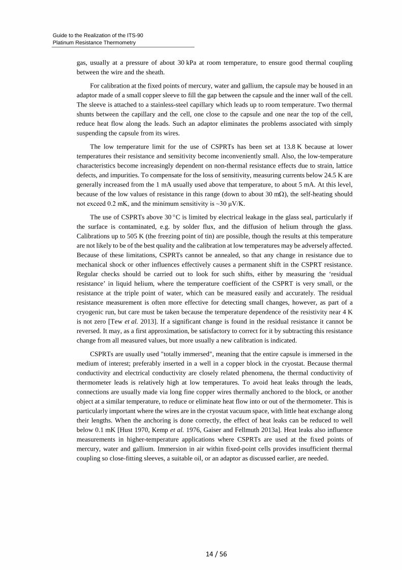
Figure 1. Schematic diagram of a typical 25 Ω capsule-type SPRT. The sensing element is
formed from fine, ~0.07 mm diameter, coiled platinum wire supported on a notched high-purity
silica cross. The four lead wires are welded to the sensing element, two at each end, and pass
through the glass seal. The platinum sheath is about 5 mm in diameter and 50 mm long.
(Illustration published on courtesy from FLUKE®)
3.2.2 Long-stem standard platinum resistance thermometer
Long-stem standard platinum resistance thermometers (LSPRTs) are applied in the temperature range
between the triple point of argon (-189.3442 °C) and the freezing point of aluminium (660.323 °C). A
typical design is shown in Figure 2. The sensor element is platinum wire of 0.05 mm to 0.1 mm
diameter, which may be wound onto the former in a variety of ways. The wound element is placed into
a fused-silica tube with a length of 480 mm to 650 mm and outside diameter up to about 8 mm. The
tube is sandblasted or blackened along part of the lower length to reduce radiative heat transfer (light-
piping) between the element and the head at room temperature. Some metal-sheathed SPRTs are also
made (see comments in Sec 5.1.1). The former for the sensing element is usually made of fused silica,
occasionally Vycor or ceramic, and in older thermometers, mica. The length of the element is typically
35 mm to 50 mm, and it has a nominal resistance at the temperature of the TPW of 25 Ω, giving the
SPRT a sensitivity of 0.1 Ω / °C.
The upper temperature limit for LSPRTs having mica formers or mica insulation is 500 °С due to
the release of water of crystallisation from the mica at higher temperatures. Once driven from the mica,
the water condenses at temperatures near 0 °C causing electrical leakage and measurement errors.
Above 660 °C, LSPRTs with silica insulators exhibit an exponentially increasing electrical breakdown
of the insulation that can lead to errors of a few tens of millikelvin at 960 °C (see Subsection 3.2.3).
Mechanical problems can also arise due to the large difference between the thermal-expansion
coefficients of platinum and fused silica, leading to mechanical deformation and short circuits either in
the sensor element or between lead wires.
Figure 3 shows two of the most frequently used designs of the resistance element of LSPRTs.
Because the plasticity of platinum increases sharply at temperatures above 200 °С, the sensor element
should have a design that prevents the coil from sliding along the former and causing short-circuiting
of the wire turns. Four platinum leads with a diameter of 0.2 mm to 0.4 mm connect the resistance
element to the external copper cable and connections. The lead wires are usually kept apart by silica
(or mica) discs. In some designs, the leads may be placed into separate fused silica capillaries to prevent
short-circuiting. The silica or mica discs also reduce convection within the thermometer.
Guide to the Realization of the ITS-90
Platinum Resistance Thermometry
16 / 56
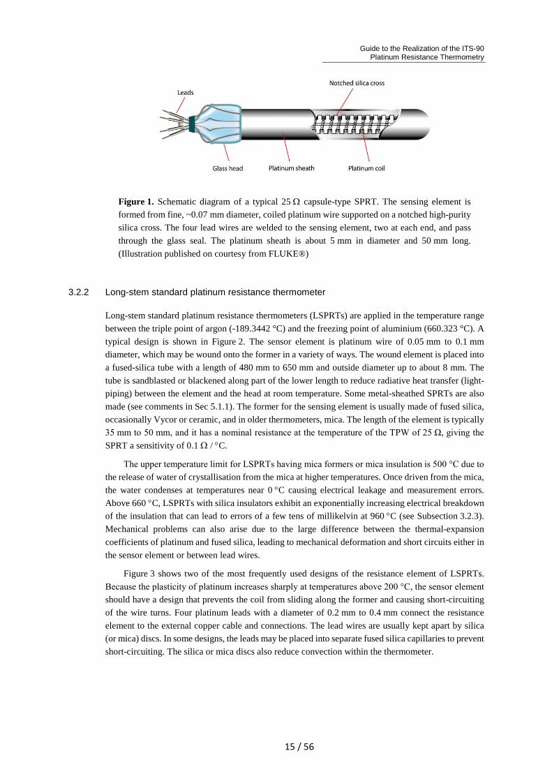
Figure 2. Schematic diagram of a typical 25 Ω LSPRT. The sensing element is a platinum coil
with a typical length of 35 mm to 50 mm. (Illustration published on courtesy from FLUKE®)
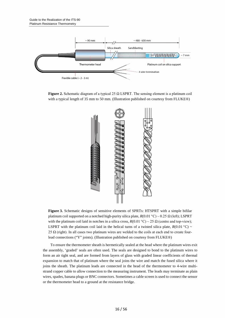
Figure 3. Schematic designs of sensitive elements of SPRTs: HTSPRT with a simple bifilar
platinum coil supported on a notched high-purity silica plate, R(0.01 °C) ~ 0.25 Ω (left); LSPRT
with the platinum coil laid in notches in a silica cross, R(0.01 °C) ~ 25 Ω (centre and top-view);
LSPRT with the platinum coil laid in the helical turns of a twisted silica plate, R(0.01 °C) ~
25 Ω (right). In all cases two platinum wires are welded to the coils at each end to create four-
lead connections (“Y” joints). (Illustration published on courtesy from FLUKE®)
To ensure the thermometer sheath is hermetically sealed at the head where the platinum wires exit
the assembly, ‘graded’ seals are often used. The seals are designed to bond to the platinum wires to
form an air tight seal, and are formed from layers of glass with graded linear coefficients of thermal
expansion to match that of platinum where the seal joins the wire and match the fused silica where it
joins the sheath. The platinum leads are connected in the head of the thermometer to 4-wire multi-
strand copper cable to allow connection to the measuring instrument. The leads may terminate as plain
wires, spades, banana plugs or BNC connectors. Sometimes a cable screen is used to connect the sensor
or the thermometer head to a ground at the resistance bridge.
Guide to the Realization of the ITS-90 Platinum Resistance Thermometry
17 / 56
The thermometer sheath in an LSPRT is usually filled with a mixture of inert gas plus oxygen at
a partial pressure of about 2 kPa. The total pressure is equivalent to one atmosphere at the maximum
temperature of the thermometer's application range. The low level of oxygen is sufficient to oxidise
metallic contaminants and hold them at grain boundaries: they might otherwise migrate into the
platinum lattice and affect the temperature dependence of the resistivity. At the same time, it limits the
formation of an oxide film on the surface of the platinum wire (see Subsection 5.1.1).
3.2.3 High-temperature standard platinum resistance thermometer
High-temperature standard platinum resistance thermometers (HTSPRTs) are designed for use in the
temperature range up to the freezing point of silver (961.78 °С). Their design is very similar to that of
LSPRTs, except that they use lower resistance sensors (with larger gauge platinum wire) in order to
reduce the effects of electrical leakage at temperatures above the freezing point of aluminium. Figure 3
shows also one design of HTSPRT sensing elements.
At temperatures approaching the silver point, the electrical conductivity of the fused silica formers
and discs, which make up the insulating components of thermometer, becomes appreciable. The effects
shunt the sensing element leading to errors of several tens of millikelvin. By reducing the resistance
R(0.01 °C) from the 25 Ω value used in LSPRTs to 0.25 Ω the influence of the unwanted shunting
resistance is reduced by a factor of 100. In practice R(0.01 °C) values ranging from 0.2 Ω to 2.5 Ω are
used. A measuring current in the range 5 mA to 10 mA is typical for HTSPRTs, which partially
compensates for the low resistance and loss of voltage sensitivity.
The shorter length of larger diameter wire (0.3 mm to 0.5 mm) used in the low-resistance sensors
simplifies the construction and has other beneficial effects. Firstly, it improves structural stability of
the element against the large difference between the thermal expansion of silica and platinum. The
differential thermal expansion also means that about 1 cm of space must be left at the bottom of the
sheath, when the thermometer is cold, to allow the platinum lead wires to expand. A second advantage
of the thicker wire is that it reduces the surface/volume ratio of the wire, which slows the impact of
contaminants, making the thermometer more stable, and reduces the effects of oxidation at the surface
of the wire.
At the higher temperatures, metals and other potential contaminants of platinum become
increasingly mobile and volatile, with some contaminants able to diffuse through the silica sheath.
Cleanliness of the sheath and preventing metallic contamination of the sensor element is critical for
long-term reliability of HTSPRTs.
Guide to the Realization of the ITS-90
Platinum Resistance Thermometry
18 / 56
4 STANDARD PLATINUM RESISTANCE THERMOMETER USE AND CARE
4.1 Mechanical Treatment and Shipping Precautions
SPRTs are delicate instruments. Shock, vibration, or any other form of acceleration may cause the wire
to bend between and around its supports, producing strains and mechanical damage. In the worst case,
careless day-to-day handling of a thermometer over a year has been observed to increase its resistance
at the TPW by an amount equivalent to as much as 0.1 K, and on rare occasions single incidents have
caused similar changes or complete failure. Changes may be caused over long periods by an apparatus
that transmits vibrations to the thermometer, or by shipping the thermometer in an unsuitable container.
It is strongly advisable to hand-carry SPRTs to maintain the integrity of calibration. If a
thermometer must be shipped, it should first be placed in a rigid and moderately massive container that
has been lined with soft material which conforms to the thermometer shape and protects it from
mechanical shocks or vibrations. This container should then be packed in an appreciably larger box
with room on all sides for soft packing material that will substantially attenuate any shocks that might
occur during shipment.
4.2 Thermal Treatment and Annealing
Generally, the greatest mechanical damage to thermometers occurs during manufacture and shipping.
While thermometers are annealed in the process of their production, this annealing is not always
sufficient. Therefore, with new SPRTs and SPRTs recently shipped, it is advisable to measure first the
resistance at the TPW and then beginning annealing.
LSPRTs (used up to 660 °C) should be placed in an auxiliary furnace at 480 °C to 500 °C before
the temperature is increased to about 675 °C over a period of about 45 minutes to 60 minutes. The
LSPRT is then annealed at this temperature for four hours. Afterwards, the temperature is reduced
again to about 480 °C over a 4 hour period, after which the PRT is removed directly from the furnace
to the room-temperature environment and, as soon as practical, measured at the TPW. If, after
annealing, the resistance of the sensitive element has not changed by more than 0.5 mK temperature
equivalent, it is ready for use. If the change of resistance is significant, annealing should be repeated.
If the resistance increases after each annealing cycle, the thermometer is probably contaminated or
affected by three-dimensional oxidation and should not be used.
HTSPRTs (used up to 962 °C) are annealed in the same way, but the annealing temperature
is 975 °C and they are annealed for four to six hours. After annealing they should be cooled slowly to
480 °C at no more than 50 °C per hour. At high temperatures, the SPRTs become particularly sensitive
to thermal and mechanical shock and should be handled very carefully.
To remove the defects and strain caused by normal handling, annealing should be performed
before LSPRTs are employed at the aluminium freezing point or HTSPRTs at the silver freezing point.
After an annealing period of about 30 minutes the SPRT should be transferred quickly, but gently, into
the fixed-point cell. After completion of the measurements at these fixed points, the SPRTs should be
again transferred to an annealing furnace at a temperature of about 675 °C (LSPRTs) or 975 °C
(HTSPRTs), maintained at that temperature for at least 30 minutes, and then cooled slowly to near
480 °C to restore the low-temperature vacancy concentration. From this temperature, the SPRT must
be removed relatively quickly (< 10 minutes) from the furnace into the room-temperature environment
to prevent oxidation and measured at the TPW as soon as possible to ensure that the two measurements
Guide to the Realization of the ITS-90 Platinum Resistance Thermometry
19 / 56
performed for the determination of the resistance ratio W are obtained in the same oxidation state of
the platinum sensor.
With measurements above the aluminium freezing point, great care must be taken to avoid
contamination of SPRTs by metallic impurities, and some means of protecting the thermometer may
be required. Sometimes a platinum foil layer is inserted or sapphire tubes are used.
No preliminary treatment of CSPRTs is necessary. The stability of the thermometer is checked by
monitoring its resistance at the triple point of water, and also its resistance at a low temperature, such
as 4.2 K or at the triple point of hydrogen (see Subsection 3.2.1).
4.3 Devitrification
The sheaths of LSPRTs and HTSPRTs are usually made from fused silica; silica in a glassy state that
is largely impervious to most contaminants. However, there are some contaminants, notably sodium
chloride from perspiration, that cause the silica to return to its crystalline state (much like quartz, the
natural crystalline form of silica), which is an irreversible phase transition. In its devitrified state, silica
is milky white, very brittle, and permeable to gases. Devitrification tends to occur at high temperatures
and is catalytically enhanced by alkali compounds.
Before using silica-sheathed platinum resistance thermometers above 100 ºC, they should be
carefully cleaned with pure ethanol and dried with clean paper or cloth. The cleaning with diluted nitric
acid followed by washing with clear water is also suitable. This is especially important for using
HTSPRTs above 660 ºC. It serves to remove all traces of fingerprints that would otherwise trigger
devitrification at high temperatures, and may cause patterns of devitrification to become visible. The
first traces of devitrification of the outer surface of the sheath should be removed by sandblasting with
alumina powder in order to stop the process. Protection from contamination of the element and from
devitrification of the sheath becomes increasingly difficult at higher temperatures.
4.4 Calibration
4.4.1 Calibration Procedures
For the lowest uncertainties, SPRTs should always be calibrated in their most reproducible state; that
is, the resistance should correspond to the zero-current resistance when the SPRT is in an unoxidised
state, and with an equilibrium concentration of vacancies. While this state is generally not entirely
accessible to CSPRTs, it is the ideal operating state of LSPRTs and HTSPRTs.
Before the calibration begins, LSPRTs and HTSPRTs should be annealed until the R(0.01 °C)
value is stable; typically within 0.2 mK for a LSPRT, and 0.8 mK for a HTSPRT. Once the SPRT is
stable, fixed-point measurements should be made progressing from the highest temperatures to the
lowest temperatures. For LSPRTs and HTSPRTs and fixed points temperatures below and including
the zinc point, the W values for the fixed points should be calculated using TPW measurements made
in the same oxidation state as during the fixed-point measurement. This means doing a TPW
measurement within a few hours after the fixed-point measurement. If the slow cool-down from a high
temperature is run overnight and continues much below 480 °C, the SPRT should be re-heated to
480 °C for 1 hour, and then removed to room temperature before the TPW measurement is made.
Guide to the Realization of the ITS-90
Platinum Resistance Thermometry
20 / 56
Where corrections to fixed point resistance measurements are required, such as for self-heating,
hydrostatic pressure, gas pressure, impurity, or isotope effects, they should be made to the measured
resistance values, before the ITS-90 interpolating equations are applied.
4.4.2 Consistency checks
SPRT calibrations involve a large number of measurements and corrections with considerable
opportunity for operator mistakes, either in the signs of corrections, or operating conditions of the fixed
points, or in the values of standard resistors. Therefore, it is helpful to include a number of checks in a
procedure to build confidence and reduce the chances of making mistakes.
As much as is possible, validated software should be used for making the corrections and
calculating the various W values from the bridge ratio measurements and standard resistor values. The
software should be validated using either synthetic data (including pressure corrections, etc.), or older
data from a real SPRT that has been checked using independent software or a calculator.
Where possible, a sequence of fixed-point measurements should include repeat measurements or
additional fixed points as a redundancy check. Some laboratories use the indium point as the redundant
point for LSPRT and HTSPRTs, to check that the value of Wr,In deduced from the measured WIn is
close to the ITS-90 reference value. Plots of the calculated deviation function ∆W versus W should also
be done. For temperatures above 50 K, the curve should have weak quadratic shape and be smooth.
When calibrating a group of SPRTs, at least one SPRT should be included for which the
calibration data are already known. Many laboratories employ check thermometers for specific fixed
points. This helps to ensure that there are no major changes in the furnace operating conditions, and
ensure the fixed-point cells have not developed leaks to atmosphere and have not become contaminated.
It is also helpful to calculate the parameter
r,
1
1i
i
i
WS
W
−=
−(25)
for each fixed point. These Si values should be very similar for all fixed points above 50 K, although
there is a step down in crossing to temperatures above 273.16 K due to a small inconsistency in the
ITS-90 definitions. (The use of the Si values for checking purposes has been proposed in [White and
Strouse 2009] applying the alternative interpolation equation (22). The near constancy of the Si values
for each SPRT is a consequence of the resistance closely following Matthiessen’s rule. This rule states
that the additional resistivity caused by lattice imperfections is nearly independent of temperature.)
The measurements of W should be checked to ensure that the SPRTs meet the ITS-90 quality
criteria (2) and (3); most SPRTs meet these criteria comfortably. Note that the two relations defined by
ITS-90 are not quite consistent: an alternative but very similar requirement is that Si values from
Equation (25), calculated for all fixed points, should be greater than 0.9994 [White and Strouse 2009].
This requirement has the advantage of being applicable to fixed points other than mercury and gallium.
Additionally, a large drop in the Si value for the silver-point measurements is a more sensitive indicator
of insulation breakdown than the ITS-90 quality criterion (4).
Guide to the Realization of the ITS-90 Platinum Resistance Thermometry
21 / 56
4.4.3 Reporting
The simplest and minimal option for the presentation of SPRT calibration data is to report the measured
W values for all of the fixed points, and their uncertainties. The uncertainties should be presented in
terms of resistance ratio, though it is helpful to give the equivalent temperature uncertainty. It is also
essential to include the coefficients for the interpolating equations realisable using those fixed points
as additional information.
It is also necessary to report the resistance value at the TPW for the SPRT. This value is required
to track the stability of the SPRT with shipping to and from the calibration laboratory. This value of
R(0.01 °C) should not be used to calculate W values: instead the user should measure the R(0.01 °C)
on their own equipment, as this minimises the propagation of uncertainties associated with the bridges
and standard resistors, and real changes in the SPRT resistance.
Appendix 2 provides a table of typical resistance ratios and sensitivity coefficients at the fixed
points, which are useful for calculating the temperature equivalents of measurement uncertainties.
5 EXPERIMENTAL SOURCES OF UNCERTAINTY
This subsection provides a brief summary of the known sources of uncertainty affecting platinum
resistance thermometry, see also the overview of factors influencing the resistance given in [Pokhodun
2002, Meyer and Ripple 2006]. The subsection explicitly excludes effects relating to fixed-point
realisations (impurities, isotope effects, hydrostatic corrections, pressure effects, etc), since sources of
uncertainty associated with fixed points are covered in Chapter 2 Fixed Points
(http://www.bipm.org/en/committees/cc/cct/guide-its90.html), and effects associated with the triple
point of water are covered in Section 2.2 Triple Point of Water of this chapter. The budget for
estimating the uncertainty of the ITS-90 realisation with SPRTs calibrated at the fixed points is
presented in Subsection 6.
5.1 Factors affecting SPRT resistance
5.1.1 Oxidation
SPRT sheaths are filled with a gas for improving the thermal coupling between the sensing element
and the sheath. In the past, dry air was widely used, but nowadays the gas consists mainly of a mixture
of an inert gas, often argon or helium, with a partial pressure of oxygen between about 2 kPa to 10 kPa.
An oxygen content of at least 1 kPa is necessary to prevent contamination of the sensing element by
metallic impurities reduced from their oxides. On the other hand, effects associated with the oxidation
of the platinum cause hysteretic changes in the SPRTs resistance. This effect is complicated further by
its dependence on the partial pressure of oxygen, the operating temperature, the presence of impurities,
and crystal size and orientation [Wang and Yeh 1998]. To reduce oxidation effects, the oxygen content
should be as small as practical. A partial pressure of oxygen of about 2 kPa is a good compromise
between the need for oxygen and its deleterious effects.
The chemical interactions between platinum and oxygen are complex, with as many as a dozen
possible oxides and allotropes. The oxides most relevant to platinum thermometry are PtO, PtO2 and
Pt3O4 [Berry 1978, 1980, 1982a, 1982b, Seriani et al. 2006, Sakurai and Tamura 2011, Jursic and
Rudtsch 2014]. Platinum oxidation has been investigated by variously applying calorimetry,
Guide to the Realization of the ITS-90
Platinum Resistance Thermometry
22 / 56
thermogravimetry, mass spectrometry, electron diffraction, acid solubility, and thermodynamic
modelling [Seriani et al. 2006, Sakurai et al. 2008, Sakurai and Tamura 2011].
For partial pressures of oxygen of a few kPa, the formation and dissociation of platinum oxides
takes place with temperature-dependent rates as follows. Up to about 350 °C, which is dependent on
the partial pressure of oxygen, less than one monolayer of oxide is formed, so the oxide is described as
two-dimensional. The rate of formation is slow, being just detectable after one hour at 200 °C, and is
still progressing after many tens of hours at 300 °C. In saturation, its temperature equivalent of the
effect amounts to about 1 mK to 2 mK in 25 Ω thermometers.
At higher temperatures, the two-dimensional oxides dissociate. But at temperature up to about
550 °C, a three-dimensional surface layer may slowly propagate deeper into the wire, apparently
limited only by diffusion and without signs of saturation. The temperature equivalent of the resistance
change may reach 10 mK or more in 25 Ω thermometers, and it depends on the heat-treating period.
This effect also depends on the partial pressure of oxygen in the exchange gas; both the rate of oxidation
and the dissociation temperature decrease as the partial pressure is decreased [Ancsin 2003]. Studies
performed by Berry (1980, 1982a, 1982b) and Sakurai and Tamura (2011) show that the formation of
the three-dimensional oxide can usually be suppressed by applying partial oxygen pressures of only a
few kPa. Heat treating the SPRTs at 600 ºC or higher will cause the three-dimensional oxide to
dissociate and should largely restore the SPRT. However, extended heat treatment for very long periods
(>> 10 hours) may be required, and in some SPRTs, the effect can be difficult to suppress. Sakurai and
Tamura (2011) have also observed anomalous phenomena that indicate a kind of irreversibility
associated with oxidation.
When oxidation effects occur in SPRTs, the relative change of the resistance ratio W(T90) is much
smaller than that of R(T90). This is caused by the fact that oxidation and dissociation change the cross-
sectional area of the platinum core, while the resistivity of the core remains unchanged. Berry (1980,
1982a) has developed a two-zone model with a relatively poorly conducting oxide film at the surface
for describing the two-dimensional effect. The moderately good stability of W with respect to oxidation
reduces the problem to a manageable level in most cases. The main difficulty for high-accuracy
measurements is that the measurements of R(T90) and R(273.16 K) used for the W(T90) calculation must
correspond to the same oxidation state, and hence R(273.16 K) must be measured frequently if the
oxidation is causing substantial drifts. Particular care may be necessary when the SPRT passes from an
oxidising to a dissociating temperature range. If a frequent measurement of R(273.16 K) is not feasible,
dedicated experiments are required to investigate the magnitude of the effects and make a reliable
estimate of the uncertainty.
5.1.2 Impurities
In an ideal metal conductor, electrical resistance is caused mainly by the scattering of electrons due to
the thermal motion of the metal atoms. Additional scattering of electrons caused by impurities gives
rise to an additional contribution to the electrical resistance, which is approximately independent of
temperature [Berry 1963]. Impurities cause irreversible changes in the resistance-temperature
dependence of SPRTs, and are a main cause of long-term drift. The impurities may originate from the
production of the wire, including insufficient purification of platinum, contamination during
preparation of the sensing element or production of the thermometer. Impurities may also originate in
the sheaths after the thermometer is assembled, by diffusion especially from metal sheaths, at
temperatures above 450 ºC. Some impurities can diffuse through fused-silica sheaths at temperatures
above about 900 °C [Marcarino et al. 1989]. For thermometers used at temperatures below 450 ºC, the
Guide to the Realization of the ITS-90 Platinum Resistance Thermometry
23 / 56
long-term drift is usually very small, no more than 1 mK with many hundreds of hours of use [Berry
1962]. Above 450 ºC the drift increases with increasing temperature and length of exposure and may
reach 5 mK/100 h at the silver point [Berry 1966, Fellmuth et al. 2005]. The form and speed of drift
depend on quantitative and qualitative composition of impurities in the platinum wire [Pokhodun et al.
2005].
5.1.3 Strain and hysteresis
Elastic strain on the platinum wire, which causes a temporary distortion of the atomic lattice, modifies
the resistance. From research on platinum strain gauges it is known that electrical resistance of platinum
increases when the wire is under tension and decreases when under compression. Strain typically arises
from differential thermal expansion between the platinum wires and its insulating supports, or from
mechanical movement of the wire, or a mixture of both. Because it is a purely elastic effect, the
deformation disappears on cessation of the mechanical forces. However, where mechanical and thermal
causes combine, the effect gives rise to hysteresis, which becomes apparent with cyclic excursions in
temperature of more than several tens of degrees.
The magnitude of the hysteresis is strongly influenced by the design of the SPRT, the materials
used in its construction, and the degree to which the platinum is allowed to expand and contract relative
to support structures. The effects are typically no more than 0.3 mK peak-to-peak, but can be as low as
0.1 mK peak-to-peak and range up to 1.8 mK peak-to-peak [Berry 1983].
5.1.4 Vacancies and defects
In a manner, very much like the effects of impurities, defects in the crystal structure of the platinum
lattice also increase the resistance of the wire. The defects may be induced thermally or mechanically.
Thermally induced defects
At temperatures above about 450 °C, the thermal motion of the atoms occasionally causes some atoms
to jump out of position in the lattice, creating vacancies (absence of an atom), interstitials (extra atom
where one shouldn’t be) or other crystal dislocations. The effect increases exponentially with rising
temperature, and at higher temperatures, is responsible for the formation of more complex, multi-atom
(higher energy) defects, corresponding to many tens of millikelvin temperature equivalent of the
resistance change at 962 °C.
Given sufficient time at any temperature, the concentration of thermally induced vacancies reaches
an equilibrium concentration, causing an increased resistance of approximately [Berry 1966]
a1200 (273.16 K) exp( / )R R E kTδ ≈ − , (26)
where Ea is the activation energy for the formation of the vacancy or defect in the lattice (≈ 1.5 eV for
simple vacancies in platinum). The additional electrical resistance caused by the vacancies is
considered to be an integral part of the R(T90) characteristic of the thermometer, but it becomes
detectable after quenching. Because the equilibrium concentration is determined by the rate at which
vacancies are created or destroyed, the rate at which the equilibrium is reached is also temperature
dependent. This means that defects anneal out according to an exponential law with a half-life, τ,
dependent on the activation energy for the defect:
Guide to the Realization of the ITS-90
Platinum Resistance Thermometry
24 / 56
0 aexp( / )E kT=τ τ , (27)
where τ0 is a time constant characteristic of the diffusion and equilibration process. For simple low-
energy vacancies, the half-life ranges from milliseconds at 960 °C to hours at temperatures below
400 °C. Thus, equilibration occurs very quickly when moving to higher temperatures but very slowly
when moving to low temperatures. If an SPRT is cooled too quickly, the vacancies can become
quenched-in and cause errors in the R(T90) characteristic at lower temperatures. Recommended cooling
rates vary but should be no more than 50 °C per hour when cooling from temperatures above 500 °C
[Mangum et al. 1990]. The annealing of defects with higher activation energies requires higher
temperatures and longer annealing times. Once the SPRT has cooled to 500 °C from higher
temperatures, the residual effects of vacancies are negligible, and the thermometers should be cooled
quickly (a few minutes) to room temperature to avoid oxidation.
Mechanically induced defects
The most troublesome defects are those arising from mechanical damage to the wire. Typically, a large
number of defects, including high-energy defects, are introduced during the cold drawing of the
platinum wire prior to the manufacture of the SPRT. Although the SPRT is thoroughly annealed at the
time of manufacture, many of the higher-energy defects will persist and be a permanent part of the
thermometer behaviour. Mechanical shock or vibration during use is a major cause of defects and,
hence, drift in SPRTs. Mechanical damage, to some degree, occurs during all use of the thermometers
with effects of the order of microkelvin accumulating each time an SPRT is knocked [Berry 1962].
Berry (1983) suggested that the mechanical damage could be classified as inelastic or plastic according
to the degree of damage it caused.
Inelastic deformation occurs when forces below the yield point of the wire are applied, but the
deformation does not disappear with cessation of the mechanical force. The SPRT can be restored by
annealing, so the effect also gives rise to hysteresis. Berry (1983) describes this effect as similar to
internal friction, and is probably due to the creation of low-energy defects.
Plastic deformation arises when the mechanical forces exceed the yield point of the platinum wire,
and is usually caused by mechanical shock (i.e., it is rarely due to thermal effects). It leads to strong
deformations of the crystal lattice accompanied by the generation of many defects, only some of which
will be removed by annealing.
In principle, all crystal defects can be removed with sufficient annealing [Berry 1966, 1972, Berry
and Lamarche 1970]. However, for the highest-energy defects, the annealing temperatures may be
beyond the material limits for the SPRT sheaths and support structures. In these cases, the effects of
such defects are practically irreversible. Long-term drifts in SPRTs, whether caused by impurities,
highest-energy defects or dimensional changes, are evident from changes in the R(273.16 K) values
that cannot be removed by annealing. Note that long-term downward drifts in resistance are unusual,
but may be due to insufficient annealing during manufacture.
Some of the causes of long-term drift effects can be distinguished. In particular, dimensional
changes arising from plastic deformation, volatilisation of platinum, and changes incurred during an
episode of three-dimensional oxidation, lead to a change in the resistance R(273.16 K) but not the
W(T90) value [Berry 1966] (“δR/R ≈ const. instability”). On the other hand, defects and impurities tend
to cause an increase in resistance that is more or less independent of temperature (“δR ≈ const.
instability”), so that both R(273.16 K) and W(T90) change. The resulting change of the resistance ratio
is given by the relation δW = (1-W) δR(273.16 K)/R(273.16 K).
Guide to the Realization of the ITS-90 Platinum Resistance Thermometry
25 / 56
For capsule-type thermometers, the upper temperature limit (typically 156 ºC) means defects
cannot be removed by annealing and are, therefore, practically indistinguishable from impurity effects.
A valuable (high resolution) indicator of resistance shifts in capsule-type SPRTs is the residual
resistance at liquid-helium temperature. It is therefore good practice to check it at regular time intervals.
But a careful check requires consideration of the small temperature dependence of the resistivity at
these temperatures [Tew et al. 2013].
5.1.5 Moisture
Berry (1966) and Zhang and Berry (1985), established that the electrical insulation resistance of mica-
insulated SPRTs deteriorates once the thermometer has been used much above 500 °C for an extended
period. Marcarino et al. (1999) subsequently demonstrated an effect as large as 1 mK or more. The
problem is caused by the release of water of crystallisation from the mica when the SPRT is exposed
to high temperatures. Quartz insulated SPRTs may also exhibit a moisture effect due to the small
quantities of water trapped within the sheath during manufacture, although the effect is usually much
smaller than for mica. The effect of the water is greatest near 0 °C, where it condenses or freezes on
the internal surfaces of the SPRT. The effect decreases exponentially as the temperature moves away
from 0 °C [Berry 1966]. As the temperature decreases below 0 °C, the conductivity of the ice falls,
while above 0 °C an increasing fraction of the water is vapour. At -39 °C, the effect is very much
reduced and by 200 °C the effect is negligible.
SPRTs affected by moisture typically exhibit long (> 10 minutes) settling times, and sometimes
instability at the TPW. They will also exhibit hysteresis due to the migration of moisture within the
sheath, which may be confused with oxidation effects. The effect may be sensitive to the operating
frequency of the resistance bridge, so it is sometimes detectable by changing the frequency (current-
reversal times for dc bridges) [Marcarino et al. 1999].
The presence of moisture can be assessed by using dry ice to cool the upper end of the SPRT
sheath with the SPRT in a water triple point cell. The dry ice condenses the moisture away from the
electrically conducting elements of the SPRT. The observed change in the triple-point resistance
typically ranges from undetectable for good quartz SPRTs to 100 µK or more for older mica-insulated
SPRTs.
5.1.6 High-temperature insulation breakdown and contamination
At sufficiently high temperatures, all of the insulating materials used in SPRTs show the thermistor-
like decrease in electrical resistivity characteristic of large-band-gap semiconductors. The resistance
decreases exponentially with temperature, causing significant effects in 25 Ω SPRTs at temperatures
above 700 °C and inducing errors as large as 400 mK at 960 °C. Berry (1995) and earlier Zhang and
Berry (1985) investigated the effect and demonstrated a complex dependence on a variety of influence
variables, including:
• The electrical operating conditions, including any ground and screen configuration of the
measurement circuit, grounding or screening of components in the fixed-point furnace, any dc
polarising voltage, and the time that the SPRT is subjected to the polarising voltage.
• The structure of the thermometer, including the insulator material, the geometry of the insulator
material and the platinum winding, and contact between the platinum winding and the insulator.
Guide to the Realization of the ITS-90
Platinum Resistance Thermometry
26 / 56
• Thermal operating conditions including the temperature distribution along the thermometer sheath
and the thermal history.
There are also peculiar effects, similar to the electrical charge and discharge of batteries, associated
with the insulation [Berry 1995, Moiseeva 2005]. White et al. (2007) and Yamazawa et al. (2007)
showed that most of the observed complexity is explained by the influence of metal-semiconductor
diodes (also known as Schottky-barrier or point-contact diodes) formed at the points of contact between
the platinum and the silica insulators in the SPRT. It also seems likely that the conduction in fused
silica is ionic rather than electronic, being due to impurities, which explains the battery-like effects. In
practice, the leakage effect is far more complicated than a single conductance in parallel with the SPRT
resistance. There are conductances distributed between each of the leads along the full length of the
thermometer, each subject to different voltages and temperature profiles. Additionally, there are shunt
resistances and voltage differences between the SPRT and the furnace.
Evans (1984) estimated the magnitude of both internal and external (through the sheath) leakage,
and showed that guarding helps suppress some leakage resistance effects for several major models of
thermometer. Berry (1995) showed that a dc offset of the correct polarity (approximately +6.4 V
between thermometer wires and ground), applied to the measurement circuit or to conducting screens,
allows to reduce significantly the conductance of the shunt (the resistance is increased). Some
resistance bridges have the facility for introducing the offset. Recent experiments [Widiatmo et al.
2013] suggest this may be a way of switching the platinum-silica diodes off so that the leakage
resistance effect can be measured.
Measurements of the shunt resistance by many workers, e.g. [Pokhodun et al. 1990, Berry 1995,
Yamazawa and Arai 2003, 2005, Moiseeva 2005], suggest that typical values for a lumped shunt
resistance, in the absence of a dc bias, for thermometers with quartz insulation are in the range 0.5 MΩ
to 20 MΩ at 960 °C, which produce leakage effects of 3 mK to 0.08 mK for a sensor with
R(273.16 K) = 0.25 Ω. Note that this effect may increase or decrease following calibration, when the
thermometer is in use, depending on the temperature profiles along the thermometer sheath. These
observations suggest a standard uncertainty of the order of 1 mK at 960 °C for 0.25 Ω thermometers.
For thermometers employing glass and/or mica insulation, the leakage conductance is much greater
and becomes apparent at lower temperatures with errors of about 1 mK at 600 ºC.
During the calibration of HTSPRTs at the silver freezing point, the diffusion of silver through
quartz may lead to contamination of the platinum sensing element. Different attempts to utilize passive
barriers (glassy carbon crucible, sapphire thermowell, platinum sheath) and dc electric fields to protect
the HTSPRTs from silver have been described [Hill 2015].
5.2 Thermal effects arising in use
5.2.1 Conduction and immersion effects
Static temperature-measurement errors are caused by the sensing element of the SPRT not being in
direct thermal contact with the object of interest. The temperature indication of the thermometer is in
practice affected by the many thermal conductances between the sensor and neighbouring objects.
These include the axial thermal conductances of the measuring leads and the sheath, which extend to
room temperature for LSPRTs and HTSPRTs, and the radial thermal conductance, which is influenced
by the thermal conductivity of the exchange gas and the sheath and the heat-transfer coefficient between
Guide to the Realization of the ITS-90 Platinum Resistance Thermometry
27 / 56
the sheath and its environment. A low radial thermal conductance also means a high self-heating effect,
see Subsection 5.3.3.
The thermometer immersion problem has been investigated theoretically in [White and
Jongenelen 2010, Gaiser and Fellmuth 2013a and 2013b] and experimentally, for instance, in [White
and Jongenelen 2010, Riddle et al. 1973]. It has been shown that after the whole sensing element is
immersed in the temperature environment to be measured, the static temperature-measurement error
decreases exponentially with further immersion. The immersion characteristic can be used
experimentally to estimate the residual errors. A thermometer is sufficiently immersed when there is
no detectable change in the indicated temperature with additional immersion in a constant-temperature
environment.
For fixed-point measurements, the hydrostatic pressure effect must be considered (see Chapter 2
Fixed Points), the magnitude of which is given for the different fixed-point substances in Table 2 of
the text of the ITS-90. Usually the results of measurements of a fixed-point temperature are considered
as acceptable, if the SPRT immersion curve corresponds to the linear relation, describing the effect of
the hydrostatic pressure on the temperature of the solid-liquid interface, over a distance of at least
(3-5) cm from the cell bottom. The uncertainty due to the immersion effect can be evaluated with the
following equation [Strouse 2005]:
2
2 90SPRT 90 90 0 0
1
d1( ) ( ) ( ) ( )
1 d
N
i ii
Tu T T h T h h h
N h=
δ = − − − −
∑ , (28)
where N is the number of measurements of the immersion characteristic, h is the distance along the
axis of the cell, and dT90/dh is the hydrostatic-pressure coefficient given in the text of the ITS-90. The
determination of an immersion curve requires high-accuracy measurements of very small temperature
differences. It is preferable to make measurements at two measuring currents with subsequent
extrapolation of the results to the zero power in order to eliminate the influence of changes in the heat-
exchange conditions when moving the SPRT in the re-entrant well of the cell. It may be preferable to
make measurements on insertion of the SPRT, rather than on its withdrawal, because on withdrawing
the SPRT the heat transfer fluid (air, water, oil) flows down into the measurement zone, with potentially
harmful thermal effect, whereas expelling the fluid on insertion does less harm (though any vertical
movement will create some disturbance to the temperature profile along the stem, which must be
allowed to subside).
The influence of poor thermometer immersion on fixed point measurements can also be assessed
by applying to the furnace a small, ~1 K, temperature oscillation with a period of at least 30 min while
observing the plateau [Fahr and Rudtsch 2008]. The amplitude of the observed fluctuations in the
plateau temperature provides a direct measure of the coupling between the SPRT and the furnace. Note
that the value of the thermal coupling constant varies throughout the melt or freeze of the cell [Fahr
and Rudtsch 2008]. The difference between the furnace temperature and the fixed-point temperature
can be determined from the monitoring SPRT once the cell has stabilised after the freeze.
The difference between the mean temperature of the sensing element and that of the solid-liquid
interface depends on several factors: the depth of the thermometer immersion into the fixed-point cell,
the presence of a continuous interface along the height of the fixed-point substance in the cell, the
SPRT design, as well as heat exchange in the thermometer well and outside the cell. The influence of
each of these factors can be evaluated by analysing the change of the thermometer immersion curve
after a change in particular conditions during the fixed-point realisation. The depth of thermometer
immersion into the cell is generally considered to be the main factor influencing the static temperature-
Guide to the Realization of the ITS-90
Platinum Resistance Thermometry
28 / 56
measurement error. Above room temperature, the necessary depth increases with increasing fixed-point
temperature up to about 450 °C. Then it decreases slightly as heat exchange by radiation improves. At
higher temperature especially, longitudinal radiation baffles and measures to inhibit radiation piping
through the sheath are essential, see Subsection 5.2.2. For different SPRT designs, the necessary
immersion depth may differ by as much as 10 cm. Typically, about 20 cm to 25 cm of immersion (in
addition to the length of the sensing element) in an isothermal zone is required to reduce the uncertainty
component to 0.1 mK at 400 °C.
Collections of experimentally determined immersion curves are available within reports on Key
Comparisons performed with LSPRTs at the TPW (CCT-K7 [Stock and Solve 2005, Stock et al. 2006])
and at the other fixed points in the range 84 K to 933 K (CCT-K3 [Mangum et al. 2002]). In several
cases, the curves do not follow the linear behaviour corresponding to the hydrostatic-pressure
coefficient, even near to the maximum possible immersion. These departures increase the uncertainty
estimate from Equation (28). The analysis of possible causes for such deviations is somewhat easier
for the TPW because cells can be checked visually to confirm the thermometer well is completely
surrounded by a solid-liquid interface and the temperature field around the cell is homogeneous along
its height. The immersion curves of an SPRT were obtained for 23 different TPW cells with the
immersion depth varying from 205 mm to 289 mm [Stock and Solve 2005], where the completeness of
the interface was visually noticed. The analysis of immersion curves is more complicated for the other
fixed points because the position of the interface is invisible and it is difficult to control the
homogeneity of the temperature field along the cell and around the thermometer sheath. The following
tests could be helpful:
• Improvement of the thermal contact between the thermometer sheath and the re-entrant well by
introducing sleeves or contact liquids in the gap.
• Check of the influence of the temperature around the cell, e.g. by adjusting the temperature
periodically, which may allow corrections for disturbing influences [Fahr and Rudtsch 2008].
Large influences may be caused by thermal links between the thermometer well and the outer wall
of the cell. In the beginning of a freeze such links may consist of connecting spaces filled with
liquid fixed-point substance and at the end of the freeze through spaces filled with solid substance
[White and Mason 2011].
• Application of different methods for initiating an inner solid-liquid interface around the
thermometer well, on which the completeness of the interface depends [Ivanova et al. 2013, White
and Mason 2011]. In particular, it depends on the starting point of the initiation after observation
of supercooling, on the duration of the cooling with a rod inserted in the thermometer well, and on
the thermal conductivity and heat capacity of the rod that is used. A complete outer interface at the
wall of the cell forms gradually. The time necessary for this process is dependent on the
temperature around the cell.
• Check if thermometers that have transparent (glass, quartz or sapphire) sheaths are protected from
intrusive, or escaping, radiation. (Metal sheathed thermometers need no further radiation shielding,
but the heat conduction down the sheath is usually such as to require deeper immersion.)
The experimental immersion curve is in general not a reliable estimate of the temperature profile
along the axis of the thermometer well because a displacement of the thermometer leads to a change of
the profile due to its influence [Ilin 2003]. However, the slope of the immersion curve is an indicator
of the closeness of the measurement conditions to the thermal equilibrium between the solid-liquid
interface and the thermometer. During the measurements, not only the thermometer immersion depth
must be taken into account, but also the design of the furnace or bath and the chosen modes of its
operation.
Guide to the Realization of the ITS-90 Platinum Resistance Thermometry
29 / 56
A computer simulation of the heat exchange in a zinc cell during the phase transition has shown
that lifting the LSPRT by 10 cm may lead to a change in the temperature in the lower end of the
thermometer well by 0.7 mK [Batagelj 2004, Batagelj et al. 2005]. Another simulation yielded a
relationship between the change in the temperature of the upper heater of the furnace and the
temperature profile along the axis of the thermometer well at the freezing points of tin and zinc [Ivanova
and Ilin 2005]. Furthermore, the influence of the position and the dimensions of the sheath area, over
which the surface is roughened to decrease radiation effects, see Subsection 5.2.2, on the heat removal
along the thermometer was estimated. This allowed assessment of the difference between the interface
temperature and the temperature detected by the sensing element of an LSPRT [Batagelj 2004, Batagelj
et al. 2005].
In capsule-type SPRTs, there is often an additional effect due to background heat fluxes, and static
temperature-measurement errors are caused by the heat flowΦ via the sensing electrical leads and the
thermometer [Gaiser and Fellmuth 2013a]. To evaluate the errors, two thermometer parameters are
needed: the thermal resistance RT of the CSPRT between the glass seal at the thermometer head and
the sheath, and the so-called reduction factor V = (TT-TS)/(TH-TS) (TT mean temperature of the sensor
element, TS sheath and TH head temperature). These parameters have to be determined in dedicated
experiments. The error caused by the heat flow is given by TT-TM ≈ V Φ RT since the difference between
the temperature of the measuring object TM and TS can usually be made vanishingly small.
5.2.2 Radiation effects
A significant source of error, especially at high temperatures, is heat flux to and from the platinum coil,
via thermal radiation. If the sensor is in line of sight of a surface that is appreciably hotter or colder
than that being measured, the power gained or lost by thermal radiation will result in a change of its
temperature. In TPW measurements, thermal radiation from incandescent lights in the room, which
may be incident upon the emerging thermometer sheath or the inner wall of the triple point cell, can
produce an error of up to 0.2 mK [McLaren and Murdock 1966, Riddle et al. 1973]. The TPW cell
should, therefore, be immersed in a bath in which no extraneous radiation from sources above room
temperature can reach the sensor of the thermometer. If this precaution is omitted, even with radiation
entry restricted to the top of the cell, a thermometer may require an immersion below the vapour-liquid
level of 35 cm (which is seldom available), much more than the immersion of 15 cm for a thermometer
with excellent immersion characteristics, in order for it to achieve an accuracy approaching 0.05 mK.
For high-resolution measurements, such as TPW cell comparisons, opaque radiation shields can be
used to cover the SPRTs and the top of the cells to confirm the absence of any effect.
At higher temperatures, radiation escaping via the SPRT sheath will cool the sensor element and
can lead to errors as large as a few tenths of a millikelvin at 420 °C (zinc point) rising to several tens
of millikelvin at 962 °C (silver point). This heat loss is due to “light piping” through the sheath due to
total internal reflections within the wall of the thermometer sheath. This error can be substantially
reduced by roughening the lower part of thermometer sheath from just above the sensor for some 15 cm
to 20 cm by sand blasting, or by coating this part of the sheath with graphite paint [Widiatmo et al.
2006, Žužek et al. 2014]. The same heat-loss mechanism can affect the apparent temperatures of fixed
point cells that have fused silica thermometer wells. These are less easily dealt with by sand blasting
or painting but it is a fairly simple matter to arrange that they ‘see’ only opaque surfaces substantially
at their own temperature, and not suffering net loss or gain of heat.
Guide to the Realization of the ITS-90
Platinum Resistance Thermometry
30 / 56
5.3 Resistance measurement
Resistance measurements in platinum thermometry are usually made using automatic low-frequency
resistance bridges. The reading of the bridges is typically a dimensionless ratio X = R(T90)/RS, where
R(T90) is the resistance of the SPRT under the current conditions of measurement, and RS is the
resistance of a calibrated reference or standard resistor also connected to the bridge. The bridges all
employ a 4-terminal-coaxial or guarded 4-terminal definition of resistance [Awan et al. 2011] to reduce
the effect of lead resistances and stray impedances. The major sources of uncertainty associated with
the resistance measurements include the reference resistor value and its stability, and self heating of
the SPRT due to the sensing power. There are additional minor effects associated with the connecting
cables and the resistance bridge itself.
5.3.1 Resistance bridges
There are two basic types of thermometry resistance bridges in common use: ac bridges using a
sinusoidal sensing current in the frequency range 10 Hz to 90 Hz, and so-called dc bridges, which use
a low-frequency square-wave (ac) sensing current, in the range 0.01 Hz to 10 Hz. The bridges typically
have a resolution of six to nine digits and a specified uncertainty in resistance ratio between 2×10⁻⁸ and
4×10⁻⁶, corresponding to equivalent uncertainties in temperature measurements near the TPW ranging
from about 5 µK to 1 mK. Some of the sources of error within thermometry bridges and bridge
calibration methods are summarized in [White 2003]. Rudtsch et al. (2005), Strouse and Hill (2003),
and White (1997) give additional information on typical performance of some resistance bridges. The
errors in bridges can be classified as noise, large scale or ‘integral’ non-linearities (INL), and short-
range or ‘differential’ non-linearities (DNL).
The resolution of a bridge is determined by a combination of the thermal noise generated in all
resistances and amplifiers, and quantisation error due to the conversion of the signal to a digital reading
[White and Edgar 2013]. The resolution is readily measured as the standard deviation when measuring
a single stable resistance. Uncertainty due to resolution can be reduced by decreasing the operating
bandwidth of the bridge or, equivalently, increasing the measurement time or averaging many results.
Noise in the resistance measurement may also arise from electromagnetic interference (EMI),
particularly electrical noise coupled from ac furnace controllers, electric motors, and other ac resistance
bridges operating nearby on the same carrier frequency. In a bridge with resolution limited by thermal
noise, the standard deviation of measurements will change as the square root of the bandwidth or
measurement time. If EMI due to ac machinery is present then often the standard deviation may change
more rapidly or not at all. Digital interface connections between the bridge and a computer for data
acquisition can also cause interference which arises from current flow caused by differing ground
potentials between the two devices; this can be overcome by using optical interface connections.
INL are those non-linearities that change slowly and smoothly over a wide range of bridge
readings. These effects are caused by finite input and output impedances, power coefficients of
resistors, finite gains of amplifiers, and stray capacitance and resistance of sub-circuits of the bridge.
They tend to be well modelled by quadratic or cubic functions of bridge reading. With many bridges,
the INL effects are below the manufacturers’ accuracy specification and, therefore, less significant than
many other sources of uncertainty in the temperature measurement. INL errors larger than the bridge
manufacturer’s specification are usually indicative of a faulty sub-circuit within the bridge or poor
adjustment. Additionally, because the ITS-90 is defined in terms of resistance ratio, only the non-linear
bridge errors (offsets, quadratic, and cubic terms) propagate and affect the temperature measurement.
Guide to the Realization of the ITS-90 Platinum Resistance Thermometry
31 / 56
Further, if the same bridge is used for the calibration and use of an SPRT, then the SPRT interpolating
equations largely correct the INL errors of the bridge. In such cases the INL correction and uncertainty
can be omitted from the uncertainty analysis.
DNL are commonly caused by errors in the transformer windings or analogue-to-digital
converters. They may occur at every change in reading and are generally too complex to measure,
model and correct. The effects tend to be below the manufacturers’ specifications, but can increase
with time and mechanical vibration as transformer cores lose magnetic permeability, and ADC circuits
drift out of adjustment. DNL are the dominant source of uncertainty in resistance measurements for
high resolution or differential measurements (e.g., fixed-point comparisons and self-heating
measurements). The magnitude of the resulting uncertainty can be inferred from the standard deviation
of residual error in the calibration curves for bridges.
5.3.2 Reference resistor
The two main contributions to the uncertainty in the value of the standard resistance, RS, are caused by
the calibration uncertainty (the value of the resistance) and the temperature dependence of RS. The
effects can be evaluated using a model of the temperature dependence of the resistance:
[ ]S bath S cal bath cal( ) ( ) 1 ( )R T R T T T= + −β , (29)
where Tbath is the temperature of the oil or air bath used to maintain the resistor during use, Tcal is the
temperature of the bath used to maintain the resistor when it was calibrated, and β is the temperature
coefficient of the resistor at Tcal. β is normally expressed as the fractional change per degree; i.e.,
s
s 90
d1
d
R
R T=β , (30)
with typical values for good-quality resistors within the range ±5×10⁻⁶/ºC. If the resistor is not
maintained at its calibration temperature, then a correction can be applied using (29). The cumulative
uncertainty in the resistance value due to these terms is
2 2 2 2 2 2 2S S,cal S bath cal bath( ) ( ) ( ) ( ) ( )u R u R R T T u u T = + − + β β , (31)
where u(RS,cal) is the calibration uncertainty as supplied by the electrical calibration laboratory, u(Tbath)
is the uncertainty arising from fluctuations in the resistor-bath temperature, and u(β) is the uncertainty
in the temperature coefficient of the resistor. Where Tbath and Tcal are nominally equal, the uncertainty
in the temperature coefficient can usually be ignored, as can any quadratic temperature dependence of
RS in Equation (29). Also, where the same resistance bridge is used for the two resistance measurements
used to calculate the W(T90) value (Equation (1)), uncertainty in the value of RS can be ignored and
only the stability of RS needs be considered. The uncertainty in the RS does need to be considered where
the R(0.01 °C) value of a thermometer is reported.
The calibration value for the standard resistor, RS,cal, is nearly always the dc value. If the resistor
is to be used with an ac bridge, standard resistors with a low ac-dc difference should be used [Wilkins
and Swan 1970]. For frequencies below 100 Hz, ac-dc differences arise from stray inductance and
capacitance, dielectric absorption, and eddy current effects. Errors in dc and low frequency
Guide to the Realization of the ITS-90
Platinum Resistance Thermometry
32 / 56
measurements can arise from thermoelectric EMFs produced as a result of Peltier heating at the
connections [Kirby and Laubitz1973], but these are usually small. Some standard resistors exhibit
relative ac-dc differences as large as 10-5. With resistors of the Wilkins’ design, the relative uncertainty
due to ac-dc difference, u(δRS,ac-dc/RS), see Table 3 in Subsection 6.1.1, is below 10-7.
In bridges based on dc current comparators (see for example [McMartin and Kusters 1966]), the
current i0 through the standard resistor changes with bridge reading. This causes variable power
dissipation in the standard resistor and an error with a cubic dependence on the measured resistance
ratio, X = R(T90)/RS:
3
2 2 390 S Spower 0 S 0 S
S S S
( ) 1 1R T R RX i R i R X
R R P R P
∂ ∂δ = − = −
∂ ∂ , (32)
where P is the power dissipated in the standard resistor, and the term involving the derivative is the
power coefficient. Electrical calibrations of standard resistors are normally carried out at a specified
power. The power coefficient is the product of the temperature coefficient and the thermal resistance
between the resistor windings and the environment, so good quality standard resistors are generally
quite bulky devices. The Wilkins’ type resistors [Wilkins and Swan 1970] have a power coefficient of
less than 4×10⁻⁶/W. The error is then much less than 1 µK. But this error can be considerably larger if
a purpose-built standard resistor is not used. If sufficient time is allowed for the resistor to stabilise
after current changes (tens of minutes), the effect is compensated by the self-heating correction for the
SPRT.
Considering also the uncertainty components due to ac-dc differences and the power dissipation,
from Equation (31) it follows:
2 2 2 2 2 2 2 2 2S S,cal S bath cal bath S,ac-dc S,power( ) ( ) ( ) ( ) ( ) (δ ) (δ )u R u R R T T u u T u R u R = + − + + + β β (33)
5.3.3 Self heating
Measurements with resistance thermometers necessarily involve passing a current through the
thermometer sensing element, which gives rise to Joule heating. As a result, the sensing element warms
to a slightly higher temperature than that of the object or environment whose temperature is to be
measured. The warming continues until the temperature difference is sufficient to dissipate the heat
and the steady state is reached. Considering SPRTs, most of the heat flows by conduction through the
filling gas to the sheath, though there is some convection and also conduction through solid
components. This internal so-called “self-heating” is fixed by the design of the thermometer, but there
is also an external effect between the sheath and the heat sink (for example, the liquid-solid interface
in a fixed-point cell) [Riddle et al. 1973], which in a well-designed experiment can be made relatively
small.
The self-heating effect depends on the thermal conductance between the sensor and the
measurement environment, and is therefore a useful indicator of whether good thermal contact has been
achieved, and subsequently for routine checks. Influencing factors are the design of the sensor element,
the thermal conductivity of the exchange gas, and the heat transfer to the heat sink, i.e. the solid-liquid
interface of the fixed-point material. Thus, the magnitude of the effect has to be checked individually
for each experimental setup. It is not alone determined by the parameters of the SPRT. The
measurement current must be chosen so as to achieve good resolution without excessive self heating.
For 25 Ω SPRTs the current is often 1 mA (dissipation of 25 μW at 0 °C) and the self heating effect in
Guide to the Realization of the ITS-90 Platinum Resistance Thermometry
33 / 56
a TPW cell is typically between 0.2 mK and 4 mK. With modern resistance bridges, a temperature
resolution of < 0.1 mK is easily achieved. Self heating has usually a typical variation with temperature,
showing a maximum slightly above 200 °C.
The self-heating effect is determined by making measurements at two currents and calculating the
temperature rise from the change in measured resistance. The user then has a choice of whether or not
to apply a correction for the effect. If a thermometer is measured using the same current as was used in
its calibration, and if the external conditions for the SPRT are also similar, then the effect will be similar
and the thermometer can be used without making corrections. This is convenient and is common
practice in secondary-level calibrations and measurements.
For precise work, self-heating corrections must be applied [Batagelj et al. 2003a, 2003b]. Since
the power dissipated increases as the square of the current, the resistance at zero current, R0, can be
calculated from resistance measurements R1, and R2 made using measuring currents i1 and i2 using the
following relation:
2 22 1 1 2
0 2 21 2
R i R iR
i i
−=
−. (34)
Commonly, the current ratio i2/i1 is chosen to be √2. In that case a simple measurement sequence
i1 : i2 : i1 allows the zero-current resistance to be determined from the corresponding measurements
R1 : R2 : R3 as R0 = R1 + R3 – R2. Pearce et al. (2012, 2013) have shown that the uncertainty in the
extrapolation to zero current is minimised if the current ratio is 2 and the measurement time is
apportioned in the ratio 4:1:4.
The zero-current bridge ratio 0measX is calculated corresponding to Equation (34). Its uncertainty
can be estimated using the equation:
4 42 0 2 2 22 1
meas DNL noise S2 2 22 1
4 4 2 22 1 21 2 1 1 2 2meas meas2 2 4 2 2
1 22 1 1 2
( ) [ (δ ) 2 (δ ) ( )]( )
2 ( ) ( , ) ( )[ ] 2
( )
i iu X u X u X u R
i i
i i u i u i i u iX X
i ii i i i
+= + +
−
+ − + +
−
. (35)
In Equation (35), u(δXDNL) is the uncertainty component due to the DNL error between the
measurements of 1measX and 2
measX with the two currents i1 and i2, u(δXnoise) is the component due to
electrical noise, which is assumed to have the same order of magnitude for both currents, and u(i1,i2) is
the estimated covariance associated with i1 and i2. If the relative errors of the two currents are equal,
i.e. if they are fully correlated, the second term vanishes.
5.3.4 Connecting cables and lead resistances
Figure 4 shows a simplified equivalent circuit for the measurement of a 4-terminal resistance, which
includes the finite shunt resistance of the connecting cables. The model can also be used to characterise
the input and output impedances of the bridge, hence the following nomenclature: Rout is the resistance
shunting the current source i0, and Rin is the resistance shunting the voltage measurement Vm. The
equivalent circuit also includes the lead resistances RL in each of the four leads to the measured
resistance. Analysis of Figure 4 shows that the error in the measured resistance ratio (the bridge
reading), X, is well approximated by
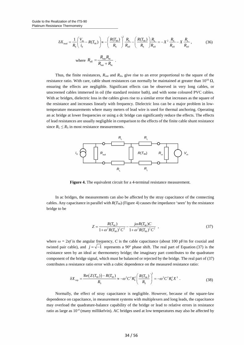
Guide to the Realization of the ITS-90
Platinum Resistance Thermometry
34 / 56
2
290 S 90 Sm L Llead 90
S 0 S eff S eff eff eff
( ) ( )1( )
R T R R T RV R RX R T X X
R i R R R R R R
δ = − ≈ − − = − −
, (36)
where out in
eff
out in
R RR
R R=
+ .
Thus, the finite resistances, Rout and Rin, give rise to an error proportional to the square of the
resistance ratio. With care, cable shunt resistances can normally be maintained at greater than 1010 Ω,
ensuring the effects are negligible. Significant effects can be observed in very long cables, or
unscreened cables immersed in oil (the standard resistor bath), and with some coloured PVC cables.
With ac bridges, dielectric loss in the cables gives rise to a similar error that increases as the square of
the resistance and increases linearly with frequency. Dielectric loss can be a major problem in low-
temperature measurements where many meters of lead wire is used for thermal anchoring. Operating
an ac bridge at lower frequencies or using a dc bridge can significantly reduce the effects. The effects
of lead resistances are usually negligible in comparison to the effects of the finite cable shunt resistance
since RL ≤ RS in most resistance measurements.
Figure 4. The equivalent circuit for a 4-terminal resistance measurement.
In ac bridges, the measurements can also be affected by the stray capacitance of the connecting
cables. Any capacitance in parallel with R(T90) (Figure 4) causes the impedance ‘seen’ by the resistance
bridge to be
90 90
2 2 2 2 2 290 90
( ) ( )
1 ( ) 1 ( )
R T j R T CZ
R T C R T C= −
+ +
ω
ω ω , (37)
where ω = 2πf is the angular frequency, C is the cable capacitance (about 100 pF/m for coaxial and
twisted pair cable), and 1j = − represents a 90º phase shift. The real part of Equation (37) is the
resistance seen by an ideal ac thermometry bridge; the imaginary part contributes to the quadrature
component of the bridge signal, which must be balanced or rejected by the bridge. The real part of (37)
contributes a resistance ratio error with a cubic dependence on the measured resistance ratio:
( )3
90 90 2 2 2 2 2 2 390cap S S
S S
Re ( ) ( ) ( )Z T R T R TX C R C R X
R R
− δ = ≈ − = −
ω ω . (38)
Normally, the effect of stray capacitance is negligible. However, because of the square-law
dependence on capacitance, in measurement systems with multiplexers and long leads, the capacitance
may overload the quadrature-balance capability of the bridge or lead to relative errors in resistance
ratio as large as 10-4 (many millikelvin). AC bridges used at low temperatures may also be affected by
i0 Rout
R(T90)
RL
Rin
Vm
RL
RLR
L
Guide to the Realization of the ITS-90 Platinum Resistance Thermometry
35 / 56
the self-inductance of any long high-resistance lead wires used for thermal anchoring. In principle, the
measured resistance is independent of the inductance (unlike the case for capacitance). However, the
large quadrature signal can overload the bridge leading to excessive noise.
For dc resistance bridges the effect of stray capacitance is complicated by the many harmonics in
the ‘square-wave’ sensing current, but normally below the limit of detection. Where detectable, it is
apparent with changes in the current-reversal times and settling times [Zhang and Berry 1985].
In systems with short leads, most cable effects can be reduced to negligible levels with care. If
the effects are significant they are often indicative of fault conditions.
6 UNCERTAINTY IN SPRT CALIBRATIONS
The estimation of the total uncertainty of a temperature value T90 realised with an SPRT
(Subsection 6.4) starts with the estimation of the uncertainty of the calibration at the fixed points
(Subsection 6.1). But for a realisation at any temperature, it is necessary to propagate the calibration
uncertainty (Subsection 6.2) and consider the non-uniqueness of the scale realisation due to
interpolation errors (Subsection 6.3). The estimation for practical measurements starts with the
calibration uncertainty as basic component. It is complex due to the variety of sub-ranges with different
interpolation equations, the option to use either single or multiple TPW measurements, possibly with
different TPW cells, and the options for the use of different resistance bridges or standard resistors for
different resistance measurements. It requires, furthermore, to consider the SPRT effects discussed in
Subsection 5 because usually a separate TPW measurement cannot be performed for each single
temperature determination. Since the practical application of SPRTs is outside the scope of this guide,
here only the most important cases routinely met during calibration of SPRTs are covered. For cases
not covered here, and for detailed explanations and derivations, see [White et al. 2018]. In all cases,
the necessary corrections and measuring errors are sufficiently small for estimating the uncertainty
using a linear mathematical model.
Some subsections below provide graphs giving numerical values for some of the uncertainty
contributions and the total uncertainty. The values in these graphs are purely indicative, and are given
only to illustrate the approximate magnitude and temperature dependence of the various contributions.
Users are expected to determine uncertainties appropriate to their measurements and use these in the
equations.
Appendix 3 gives values for the range of some of the contributions to the uncertainty in fixed-
point measurements. These values are also indicative. Most of the ranges encompass the uncertainties
reported from recent measurement comparisons, as well as the expected extremes determined from the
application of the models given in previous subsections. (For comparisons involving the TPW, see
Stock and Solve (2005), Renaot et al. (2005). For comparisons involving low temperature fixed points
(< 0 °C) and SPRTs, see Steele et al. (2002), Fellmuth et al. (2012), Head et al. (1997), Pavese et al.
(1984). For comparisons involving high-temperature fixed points (> 0 °C) and SPRTs, see Mangum
et al. (2002), Nubbemeyer and Fischer (2002).)
Guide to the Realization of the ITS-90
Platinum Resistance Thermometry
36 / 56
6.1 Uncertainty of SPRT calibration at the fixed points
6.1.1 Uncertainty in SPRT resistance at the triple point of water
The main purpose of the TPW resistance value RTPW reported on a calibration certificate is to enable
users of the SPRT to assess the stability of the SPRT and detect major changes that may have occurred
through shipping, or to detect damage that may have occurred during use. For this purpose, it is best if
the SPRT is in its most reproducible state, i.e. the SPRT is well annealed and heat-treated so that it is
strain-, vacancy-, and oxide-free. The RTPW value in this state may be different from that used for the
calculation of resistance ratios or temperature. The mathematical model for estimating the uncertainty
of RTPW is given by:
rTPW meas FP
90
d1 δ
d
WR R T
T
= +
(39)
with the measured resistance value
0meas S cal bath cal meas INL( )[1 ( )][ δ ]R R T T T X X= + − +β
(40)
and the necessary correction of the realised fixed-point temperature
8
FP FP1δ δ k
kT T
== ∑ . (41)
The individual corrections FPδ kT are explained in Table 3. Most of them were already discussed in
[Fellmuth et al. 2001, 2005, Bonnier et al. 2005].
The total Type B uncertainty in the zero-current TPW resistance, using sensing currents i1 and i2,
is
( )2
2 82 2 2 0 2 2 0 2 2rTPW S meas S INL meas S meas FP1
90
d( ) ( ) (δ ) ( ) (δ )
dk
k
Wu R R u X R u X X u R R u T
T =
= + + +
∑ , (42)
where the uncertainty of the zero-current bridge ratio 0measX is given by Equation (35) in
Subsection 5.3.3 and that of the standard resistor RS by Equation (33) in Subsection 5.3.2.
Guide to the Realization of the ITS-90 Platinum Resistance Thermometry
37 / 56
Table 3: Summary of Type B uncertainty components (Note: “No. k” indexes the terms of
Equation (41) and Appendix 3).
No. k Symbol Description of the correction Reference
1 δThyd Hydrostatic head correction Subsection 5.2.1
2 δTp Gas pressure correction ITS-90 text, Table 2
3 δTimp Influence of impurities Chapter 2, Section 2.1
4 δTiso Influence of the isotopic composition MeP-K, Technical Annex
5 δTcry Influence of crystal defects and strain Chapter 2
6 δTstat Static thermal effects Subsection 5.2
7 δTdyn Dynamic thermal effects Subsection 5.2
8 δTliq Extrapolation to the liquidus point Chapter 2, Section 2.1
δXINL Integral resistance bridge non-linearities Subsection 5.3.1
δXDNL Differential resistance bridge non-linearities Subsection 5.3.1
δRS,ac-dc ac-dc difference of the reference-resistor value Subsection 5.3.2
δRS,power Power dependence of the reference-resistor value Subsection 5.3.2
6.1.2 Uncertainty in SPRT resistance ratios at fixed points
In general, when measuring the resistance at the gallium, indium, tin, or zinc points, it is not possible
to keep the SPRT in an oxide-free state, see Subsection 5.1.1. If the SPRT is in the same oxidation state
for the measurements at fixed point i and the TPW (i = 1), the uncertainty of the resistance ratio Wi is
given by
2 2 2 2 2r, TPW,2
TPW
1( ) ( ) ( )i i i iu W u R W u R
R = + , (43)
where RTPW,i is the corresponding TPW value. If furthermore both measurements are performed with
the same reference resistor under stable conditions (negligible short-term instability), the Type B
uncertainty in the SPRT resistance for each fixed point can be estimated applying the following
equation, which considers correlations:
2
8r,2 2 2 0 2 2 2S meas, S INL TPW FP,1
90
d( ) ( ) (δ ) (δ )
d
i ki i ik
Wu R R u X R u X R u T
T =
= + +
∑ (44)
Under these conditions, the uncertainty of RTPW,i is also given by Equation (44) (i = 1).
6.2 Propagation of calibration uncertainty
The many interpolating equations of the ITS-90 greatly complicate the propagation of uncertainty for
temperatures measured using SPRTs. Complications also arise from the option to use either single or
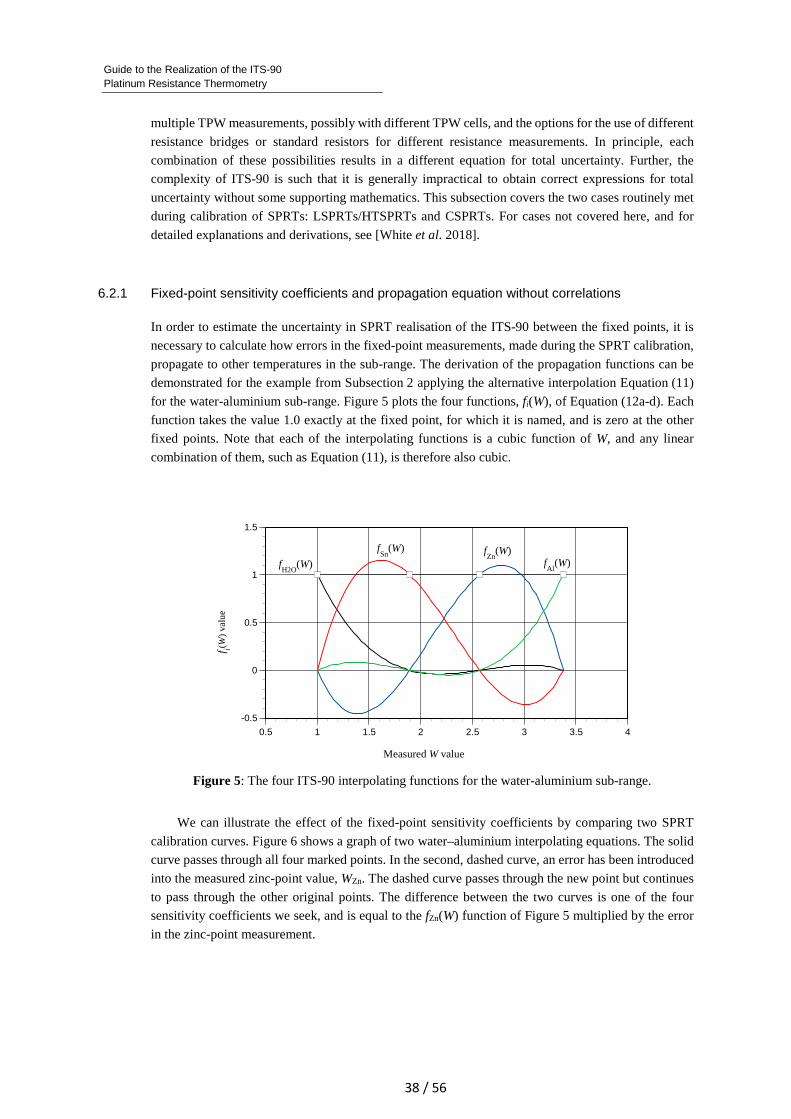
Guide to the Realization of the ITS-90
Platinum Resistance Thermometry
38 / 56
multiple TPW measurements, possibly with different TPW cells, and the options for the use of different
resistance bridges or standard resistors for different resistance measurements. In principle, each
combination of these possibilities results in a different equation for total uncertainty. Further, the
complexity of ITS-90 is such that it is generally impractical to obtain correct expressions for total
uncertainty without some supporting mathematics. This subsection covers the two cases routinely met
during calibration of SPRTs: LSPRTs/HTSPRTs and CSPRTs. For cases not covered here, and for
detailed explanations and derivations, see [White et al. 2018].
6.2.1 Fixed-point sensitivity coefficients and propagation equation without correlations
In order to estimate the uncertainty in SPRT realisation of the ITS-90 between the fixed points, it is
necessary to calculate how errors in the fixed-point measurements, made during the SPRT calibration,
propagate to other temperatures in the sub-range. The derivation of the propagation functions can be
demonstrated for the example from Subsection 2 applying the alternative interpolation Equation (11)
for the water-aluminium sub-range. Figure 5 plots the four functions, fi(W), of Equation (12a-d). Each
function takes the value 1.0 exactly at the fixed point, for which it is named, and is zero at the other
fixed points. Note that each of the interpolating functions is a cubic function of W, and any linear
combination of them, such as Equation (11), is therefore also cubic.
Figure 5: The four ITS-90 interpolating functions for the water-aluminium sub-range.
We can illustrate the effect of the fixed-point sensitivity coefficients by comparing two SPRT
calibration curves. Figure 6 shows a graph of two water–aluminium interpolating equations. The solid
curve passes through all four marked points. In the second, dashed curve, an error has been introduced
into the measured zinc-point value, WZn. The dashed curve passes through the new point but continues
to pass through the other original points. The difference between the two curves is one of the four
sensitivity coefficients we seek, and is equal to the fZn(W) function of Figure 5 multiplied by the error
in the zinc-point measurement.
-0.5
0
0.5
1
1.5
0.5 1 1.5 2 2.5 3 3.5 4
fH2O
(W)
fSn
(W) fZn
(W)fAl
(W)
Measured W value
f i(W)
val
ue
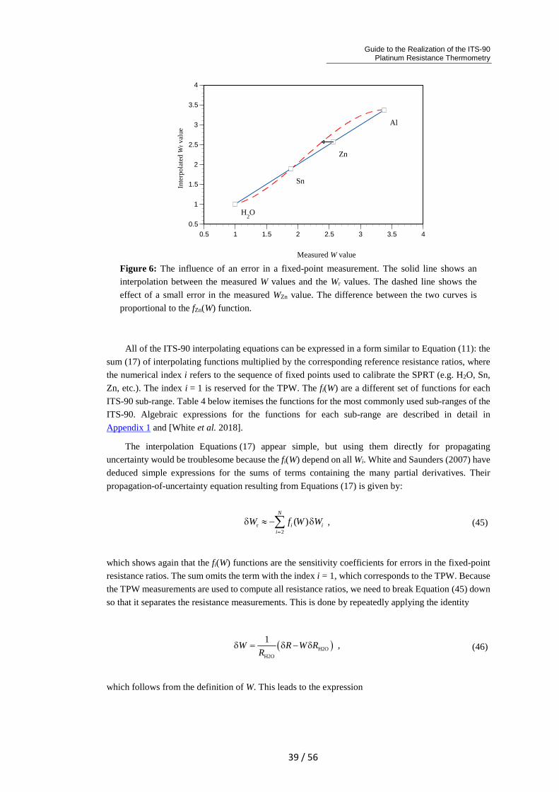
Guide to the Realization of the ITS-90 Platinum Resistance Thermometry
39 / 56
Figure 6: The influence of an error in a fixed-point measurement. The solid line shows an
interpolation between the measured W values and the Wr values. The dashed line shows the
effect of a small error in the measured WZn value. The difference between the two curves is
proportional to the fZn(W) function.
All of the ITS-90 interpolating equations can be expressed in a form similar to Equation (11): the
sum (17) of interpolating functions multiplied by the corresponding reference resistance ratios, where
the numerical index i refers to the sequence of fixed points used to calibrate the SPRT (e.g. H2O, Sn,
Zn, etc.). The index i = 1 is reserved for the TPW. The fi(W) are a different set of functions for each
ITS-90 sub-range. Table 4 below itemises the functions for the most commonly used sub-ranges of the
ITS-90. Algebraic expressions for the functions for each sub-range are described in detail in
Appendix 1 and [White et al. 2018].
The interpolation Equations (17) appear simple, but using them directly for propagating
uncertainty would be troublesome because the fi(W) depend on all Wi. White and Saunders (2007) have
deduced simple expressions for the sums of terms containing the many partial derivatives. Their
propagation-of-uncertainty equation resulting from Equations (17) is given by:
r2
( )N
i ii
W f W W=
δ ≈ − δ∑ , (45)
which shows again that the fi(W) functions are the sensitivity coefficients for errors in the fixed-point
resistance ratios. The sum omits the term with the index i = 1, which corresponds to the TPW. Because
the TPW measurements are used to compute all resistance ratios, we need to break Equation (45) down
so that it separates the resistance measurements. This is done by repeatedly applying the identity
( )H2O
H2O
1W R W R
Rδ = δ − δ , (46)
which follows from the definition of W. This leads to the expression
Measured W value
Inte
rpo
late
d W
rv
alu
e
0.5
1
1.5
2
2.5
3
3.5
4
0.5 1 1.5 2 2.5 3 3.5 4
H2O
Sn
Zn
Al
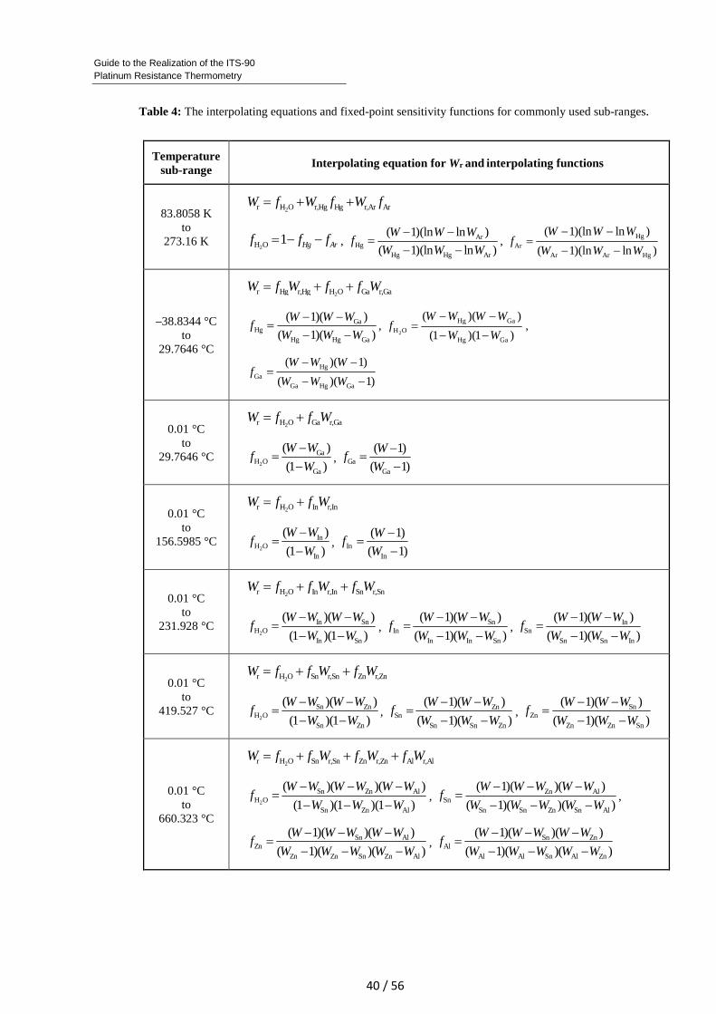
Guide to the Realization of the ITS-90
Platinum Resistance Thermometry
40 / 56
Table 4: The interpolating equations and fixed-point sensitivity functions for commonly used sub-ranges.
Temperaturesub-range
Interpolating equation for Wr and interpolating functions
83.8058 K to
273.16 K
2r H O r,Hg Hg r,Ar ArW f W f W f= + +
2H O 1 Hg Arf f f= − − , ArHg
Hg Hg Ar
( 1)(ln ln )
( 1)(ln ln )
W W Wf
W W W
− −=
− −,
Hg
Ar
Ar Ar Hg
( 1)(ln ln )
( 1)(ln ln )
W W Wf
W W W
− −=
− −
–38.8344 °C to
29.7646 °C
2r Hg r,Hg H O Ga r,GaW f W f f W= + +
GaHg
Hg Hg Ga
( 1)( )
( 1)( )
W W Wf
W W W
− −=
− −,
2
Hg Ga
H O
Hg Ga
( )( )
(1 )(1 )
W W W Wf
W W
− −=
− −,
Hg
Ga
Ga Hg Ga
( )( 1)
( )( 1)
W W Wf
W W W
− −=
− −
0.01 °C to
29.7646 °C
2r H O Ga r,GaW f f W= +
2
GaH O
Ga
( )
(1 )
W Wf
W
−=
−, Ga
Ga
( 1)
( 1)
Wf
W
−=
−
0.01 °C to
156.5985 °C
2r H O In r,InW f f W= +
2
InH O
In
( )
(1 )
W Wf
W
−=
−, In
In
( 1)
( 1)
Wf
W
−=
−
0.01 °C to
231.928 °C
2r H O In r,In Sn r,SnW f f W f W= + +
2
In SnH O
In Sn
( )( )
(1 )(1 )
W W W Wf
W W
− −=
− −,
SnIn
In In Sn
( 1)( )
( 1)( )
W W Wf
W W W
− −=
− −,
InSn
Sn Sn In
( 1)( )
( 1)( )
W W Wf
W W W
− −=
− −
0.01 °C to
419.527 °C
2r H O Sn r,Sn Zn r,ZnW f f W f W= + +
2
Sn ZnH O
Sn Zn
( )( )
(1 )(1 )
W W W Wf
W W
− −=
− −,
ZnSn
Sn Sn Zn
( 1)( )
( 1)( )
W W Wf
W W W
− −=
− −,
SnZn
Zn Zn Sn
( 1)( )
( 1)( )
W W Wf
W W W
− −=
− −
0.01 °C to
660.323 °C
2r H O Sn r,Sn Zn r,Zn Al r,AlW f f W f W f W= + + +
2
Sn Zn AlH O
Sn Zn Al
( )( )( )
(1 )(1 )(1 )
W W W W W Wf
W W W
− − −=
− − −,
Zn AlSn
Sn Sn Zn Sn Al
( 1)( )( )
( 1)( )( )
W W W W Wf
W W W W W
− − −=
− − −,
Sn AlZn
Zn Zn Sn Zn Al
( 1)( )( )
( 1)( )( )
W W W W Wf
W W W W W
− − −=
− − −,
Sn ZnAl
Al Al Sn Al Zn
( 1)( )( )
( 1)( )( )
W W W W Wf
W W W W W
− − −=
− − −
Guide to the Realization of the ITS-90 Platinum Resistance Thermometry
41 / 56
( )r H2O,2H2O
1( )
N
i i i ii
W f W R W RR =
δ = − δ − δ∑ , (47)
where RH2O,i are the TPW resistance values used to calculate each Wi . The RH2O,i value may be different
for each Wi value. From here the calculations diverge depending on how an SPRT is calibrated, in
particular, it depends on how the RH2O,i values are used, and this depends largely on the type of SPRT.
The propagation of uncertainty based on the approximate Equation (45) neglects the correlation
of the different Wi values. But the possibly resulting overestimation of the uncertainty seems to be
acceptable because primarily non-dominant uncertainty components are correlated. In most cases, the
uncertainty estimates u(Wi) are dominated by components caused by the influence of impurities on the
fixed-point temperatures, see Guide Section 2.1 Influence of impurities in Chapter 2 Fixed Points
(http://www.bipm.org/en/committees/cc/cct/guide-its90.html). This influence is not correlated
between the different fixed-point materials. A complicated program for considering correlations
completely applying the interpolation equations of the ITS-90 has been developed by Gaiţă et al. [Gaiţă
and Iliescu 2001]. But it is questionable if such a huge effort is necessary for decreasing the overall
uncertainty estimate only slightly. For most applications, Equation (47) will yield reliable uncertainty
estimates. Uncertainty propagation using the ITS-90 mathematics is also discussed in [Meyer and
Ripple 2006].
6.2.2 Propagated uncertainty
For LSPRTs and HTSPRTs, a separate TPW measurement is used to calculate each Wi value. This is
done to minimise the effects of the oxidation state of the SPRT. If we assume the uncertainties
associated with each resistance measurement in Equation (47) are not correlated, we can immediately
write down the corresponding expression for the uncertainty in the interpolated Wr value:
( )2 2 22H2O,2 2 2mean H2O
r H2O 2 22H2O H2O
( ) ( )( )( ) ( ) ( )
Ni i i
ii
u R W u Ru Ru W f W f W
R R=
+= + ∑ . (48)
The set of terms under the summation propagates the uncertainties resulting from the calibration at the
fixed points. The first term considers the mean uncertainty of the measurements at the TPW.
Equation (48) is well suited to use for the ITS-90 sub-ranges using LSPRTs and HTSPRTs, where
separate TPW measurements are used to eliminate oxidation effects. A useful feature of the equation
is that we can identify a single term that can be associated with the uncertainty in the Wi value for each
fixed point:
2 2 2H2O,2
2H2O
( ) ( )( ) i i i
i
u R W u Ru W
R
+= . (49)
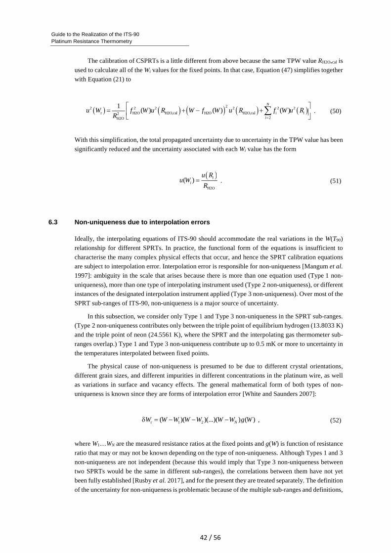
Guide to the Realization of the ITS-90
Platinum Resistance Thermometry
42 / 56
The calibration of CSPRTs is a little different from above because the same TPW value RH2O,cal is
used to calculate all of the Wi values for the fixed points. In that case, Equation (47) simplifies together
with Equation (21) to
( ) ( ) ( ) ( ) ( )22 2 2 2 2 2
r H2O H2O,cal H2O H2O,cal22H2O
1( ) ( ) ( )
N
i ii
u W f W u R W f W u R f W u RR =
= + − +
∑ . (50)
With this simplification, the total propagated uncertainty due to uncertainty in the TPW value has been
significantly reduced and the uncertainty associated with each Wi value has the form
( )
H2O
( ) i
i
u Ru W
R= . (51)
6.3 Non-uniqueness due to interpolation errors
Ideally, the interpolating equations of ITS-90 should accommodate the real variations in the W(T90)
relationship for different SPRTs. In practice, the functional form of the equations is insufficient to
characterise the many complex physical effects that occur, and hence the SPRT calibration equations
are subject to interpolation error. Interpolation error is responsible for non-uniqueness [Mangum et al.
1997]: ambiguity in the scale that arises because there is more than one equation used (Type 1 non-
uniqueness), more than one type of interpolating instrument used (Type 2 non-uniqueness), or different
instances of the designated interpolation instrument applied (Type 3 non-uniqueness). Over most of the
SPRT sub-ranges of ITS-90, non-uniqueness is a major source of uncertainty.
In this subsection, we consider only Type 1 and Type 3 non-uniqueness in the SPRT sub-ranges.
(Type 2 non-uniqueness contributes only between the triple point of equilibrium hydrogen (13.8033 K)
and the triple point of neon (24.5561 K), where the SPRT and the interpolating gas thermometer sub-
ranges overlap.) Type 1 and Type 3 non-uniqueness contribute up to 0.5 mK or more to uncertainty in
the temperatures interpolated between fixed points.
The physical cause of non-uniqueness is presumed to be due to different crystal orientations,
different grain sizes, and different impurities in different concentrations in the platinum wire, as well
as variations in surface and vacancy effects. The general mathematical form of both types of non-
uniqueness is known since they are forms of interpolation error [White and Saunders 2007]:
r 1 2( )( )(...)( ) ( )NW W W W W W W g Wδ = − − − , (52)
where W1…WN are the measured resistance ratios at the fixed points and g(W) is function of resistance
ratio that may or may not be known depending on the type of non-uniqueness. Although Types 1 and 3
non-uniqueness are not independent (because this would imply that Type 3 non-uniqueness between
two SPRTs would be the same in different sub-ranges), the correlations between them have not yet
been fully established [Rusby et al. 2017], and for the present they are treated separately. The definition
of the uncertainty for non-uniqueness is problematic because of the multiple sub-ranges and definitions,
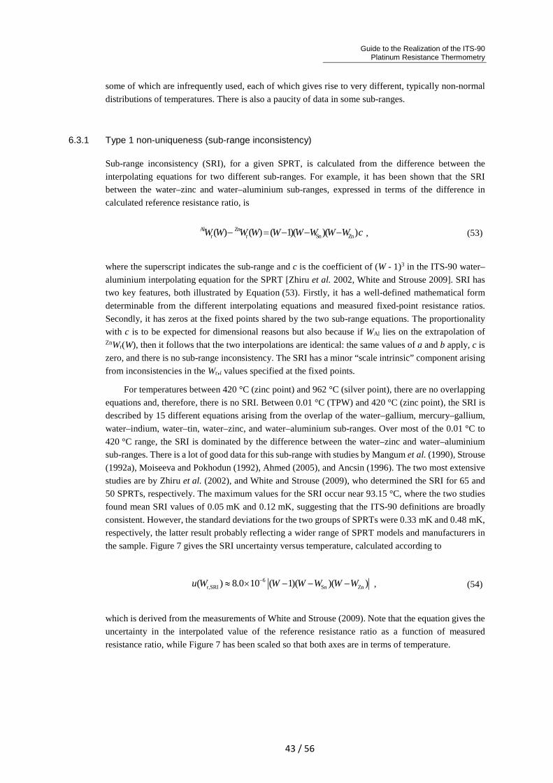
Guide to the Realization of the ITS-90 Platinum Resistance Thermometry
43 / 56
some of which are infrequently used, each of which gives rise to very different, typically non-normal
distributions of temperatures. There is also a paucity of data in some sub-ranges.
6.3.1 Type 1 non-uniqueness (sub-range inconsistency)
Sub-range inconsistency (SRI), for a given SPRT, is calculated from the difference between the
interpolating equations for two different sub-ranges. For example, it has been shown that the SRI
between the water–zinc and water–aluminium sub-ranges, expressed in terms of the difference in
calculated reference resistance ratio, is
Al Znr r Sn Zn( ) ( ) ( 1)( )( )W W W W W W W W W c− = − − − , (53)
where the superscript indicates the sub-range and c is the coefficient of (W - 1)3 in the ITS-90 water–
aluminium interpolating equation for the SPRT [Zhiru et al. 2002, White and Strouse 2009]. SRI has
two key features, both illustrated by Equation (53). Firstly, it has a well-defined mathematical form
determinable from the different interpolating equations and measured fixed-point resistance ratios.
Secondly, it has zeros at the fixed points shared by the two sub-range equations. The proportionality
with c is to be expected for dimensional reasons but also because if WAl lies on the extrapolation of ZnWr(W), then it follows that the two interpolations are identical: the same values of a and b apply, c is
zero, and there is no sub-range inconsistency. The SRI has a minor “scale intrinsic” component arising
from inconsistencies in the Wr,i values specified at the fixed points.
For temperatures between 420 °C (zinc point) and 962 °C (silver point), there are no overlapping
equations and, therefore, there is no SRI. Between 0.01 °C (TPW) and 420 °C (zinc point), the SRI is
described by 15 different equations arising from the overlap of the water–gallium, mercury–gallium,
water–indium, water–tin, water–zinc, and water–aluminium sub-ranges. Over most of the 0.01 °C to
420 °C range, the SRI is dominated by the difference between the water–zinc and water–aluminium
sub-ranges. There is a lot of good data for this sub-range with studies by Mangum et al. (1990), Strouse
(1992a), Moiseeva and Pokhodun (1992), Ahmed (2005), and Ancsin (1996). The two most extensive
studies are by Zhiru et al. (2002), and White and Strouse (2009), who determined the SRI for 65 and
50 SPRTs, respectively. The maximum values for the SRI occur near 93.15 °C, where the two studies
found mean SRI values of 0.05 mK and 0.12 mK, suggesting that the ITS-90 definitions are broadly
consistent. However, the standard deviations for the two groups of SPRTs were 0.33 mK and 0.48 mK,
respectively, the latter result probably reflecting a wider range of SPRT models and manufacturers in
the sample. Figure 7 gives the SRI uncertainty versus temperature, calculated according to
6r,SRI Sn Zn( ) 8.0 10 ( 1)( )( )u W W W W W W−≈ × − − − , (54)
which is derived from the measurements of White and Strouse (2009). Note that the equation gives the
uncertainty in the interpolated value of the reference resistance ratio as a function of measured
resistance ratio, while Figure 7 has been scaled so that both axes are in terms of temperature.
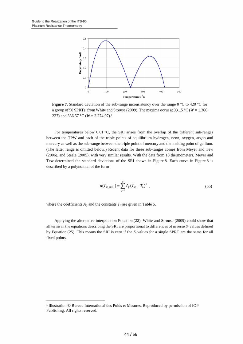
Guide to the Realization of the ITS-90
Platinum Resistance Thermometry
44 / 56
Figure 7. Standard deviation of the sub-range inconsistency over the range 0 °C to 420 °C for
a group of 50 SPRTs, from White and Strouse (2009). The maxima occur at 93.15 °C (W = 1.366
227) and 336.57 °C (W = 2.274 97).1
For temperatures below 0.01 °C, the SRI arises from the overlap of the different sub-ranges
between the TPW and each of the triple points of equilibrium hydrogen, neon, oxygen, argon and
mercury as well as the sub-range between the triple point of mercury and the melting point of gallium.
(The latter range is omitted below.) Recent data for these sub-ranges comes from Meyer and Tew
(2006), and Steele (2005), with very similar results. With the data from 18 thermometers, Meyer and
Tew determined the standard deviations of the SRI shown in Figure 8. Each curve in Figure 8 is
described by a polynomial of the form
5
90,SRI, 90 01
( ) ( ) ji ij
j
u T A T T=
= −∑ , (55)
where the coefficients Aij and the constants T0 are given in Table 5.
Applying the alternative interpolation Equation (22), White and Strouse (2009) could show that
all terms in the equations describing the SRI are proportional to differences of inverse Si values defined
by Equation (25). This means the SRI is zero if the Si values for a single SPRT are the same for all
fixed points.
1 Illustration © Bureau International des Poids et Mesures. Reproduced by permission of IOP Publishing. All rights reserved.
0
0.1
0.2
0.3
0.4
0.5
0 100 200 300 400 500
Temperature / oC
Un
cert
ain
ty /
mK
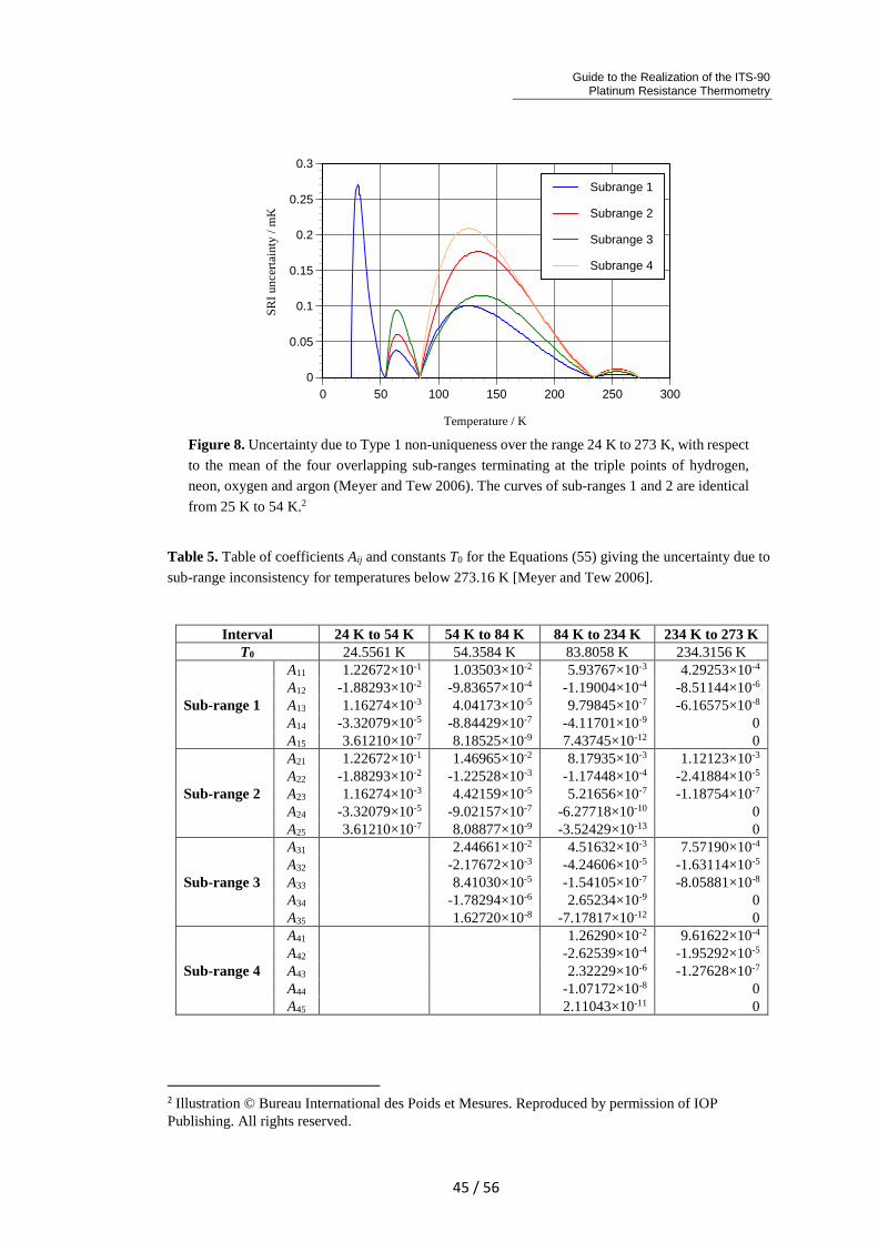
Guide to the Realization of the ITS-90 Platinum Resistance Thermometry
45 / 56
Figure 8. Uncertainty due to Type 1 non-uniqueness over the range 24 K to 273 K, with respect
to the mean of the four overlapping sub-ranges terminating at the triple points of hydrogen,
neon, oxygen and argon (Meyer and Tew 2006). The curves of sub-ranges 1 and 2 are identical
from 25 K to 54 K.2
Table 5. Table of coefficients Aij and constants T0 for the Equations (55) giving the uncertainty due to
sub-range inconsistency for temperatures below 273.16 K [Meyer and Tew 2006].
Interval 24 K to 54 K 54 K to 84 K 84 K to 234 K 234 K to 273 K T0 24.5561 K 54.3584 K 83.8058 K 234.3156 K
Sub-range 1
A11 1.22672×10⁻¹ 1.03503×10⁻² 5.93767×10⁻³ 4.29253×10⁻⁴
A12 -1.88293×10⁻² -9.83657×10⁻⁴ -1.19004×10⁻⁴ -8.51144×10⁻⁶
A13 1.16274×10⁻³ 4.04173×10⁻⁵ 9.79845×10⁻⁷ -6.16575×10⁻⁸
A14 -3.32079×10⁻⁵ -8.84429×10⁻⁷ -4.11701×10⁻⁹ 0A15 3.61210×10⁻⁷ 8.18525×10⁻⁹ 7.43745×10⁻¹² 0
Sub-range 2
A21 1.22672×10⁻¹ 1.46965×10⁻² 8.17935×10⁻³ 1.12123×10⁻³
A22 -1.88293×10⁻² -1.22528×10⁻³ -1.17448×10⁻⁴ -2.41884×10⁻⁵
A23 1.16274×10⁻³ 4.42159×10⁻⁵ 5.21656×10⁻⁷ -1.18754×10⁻⁷
A24 -3.32079×10⁻⁵ -9.02157×10⁻⁷ -6.27718×10⁻¹⁰ 0A25 3.61210×10⁻⁷ 8.08877×10⁻⁹ -3.52429×10⁻¹³ 0
Sub-range 3
A31 2.44661×10⁻² 4.51632×10⁻³ 7.57190×10⁻⁴
A32 -2.17672×10⁻³ -4.24606×10⁻⁵ -1.63114×10⁻⁵
A33 8.41030×10⁻⁵ -1.54105×10⁻⁷ -8.05881×10⁻⁸
A34 -1.78294×10⁻⁶ 2.65234×10⁻⁹ 0A35 1.62720×10⁻⁸ -7.17817×10⁻¹² 0
Sub-range 4
A41 1.26290×10⁻² 9.61622×10⁻⁴
A42 -2.62539×10⁻⁴ -1.95292×10⁻⁵
A43 2.32229×10⁻⁶ -1.27628×10⁻⁷
A44 -1.07172×10⁻⁸ 0A45 2.11043×10⁻¹¹ 0
2 Illustration © Bureau International des Poids et Mesures. Reproduced by permission of IOP Publishing. All rights reserved.
0
0.05
0.1
0.15
0.2
0.25
0.3
0 50 100 150 200 250 300
Subrange 1
Subrange 2
Subrange 3
Subrange 4
Temperature / K
SR
I un
cert
aint
y /
mK
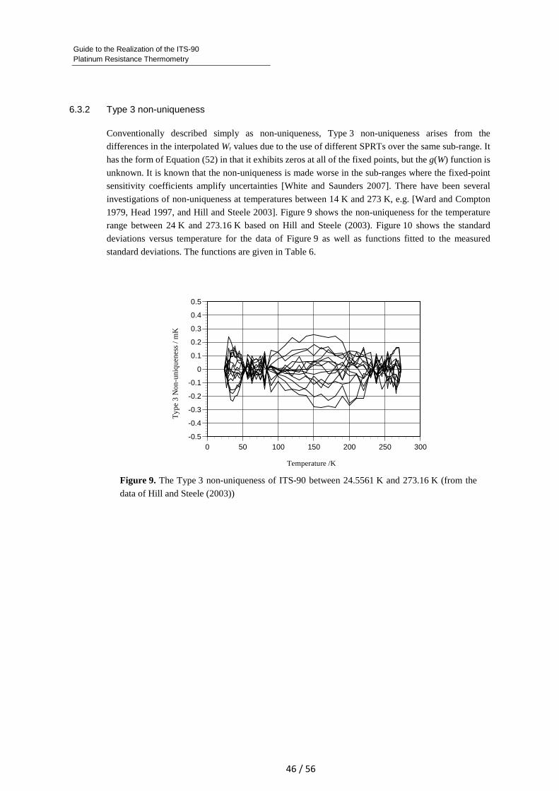
Guide to the Realization of the ITS-90
Platinum Resistance Thermometry
46 / 56
6.3.2 Type 3 non-uniqueness
Conventionally described simply as non-uniqueness, Type 3 non-uniqueness arises from the
differences in the interpolated Wr values due to the use of different SPRTs over the same sub-range. It
has the form of Equation (52) in that it exhibits zeros at all of the fixed points, but the g(W) function is
unknown. It is known that the non-uniqueness is made worse in the sub-ranges where the fixed-point
sensitivity coefficients amplify uncertainties [White and Saunders 2007]. There have been several
investigations of non-uniqueness at temperatures between 14 K and 273 K, e.g. [Ward and Compton
1979, Head 1997, and Hill and Steele 2003]. Figure 9 shows the non-uniqueness for the temperature
range between 24 K and 273.16 K based on Hill and Steele (2003). Figure 10 shows the standard
deviations versus temperature for the data of Figure 9 as well as functions fitted to the measured
standard deviations. The functions are given in Table 6.
Figure 9. The Type 3 non-uniqueness of ITS-90 between 24.5561 K and 273.16 K (from the
data of Hill and Steele (2003))
-0.5
-0.4
-0.3
-0.2
-0.1
0
0.1
0.2
0.3
0.4
0.5
0 50 100 150 200 250 300
Temperature /K
Ty
pe
3 N
on
-un
iqu
enes
s /
mK
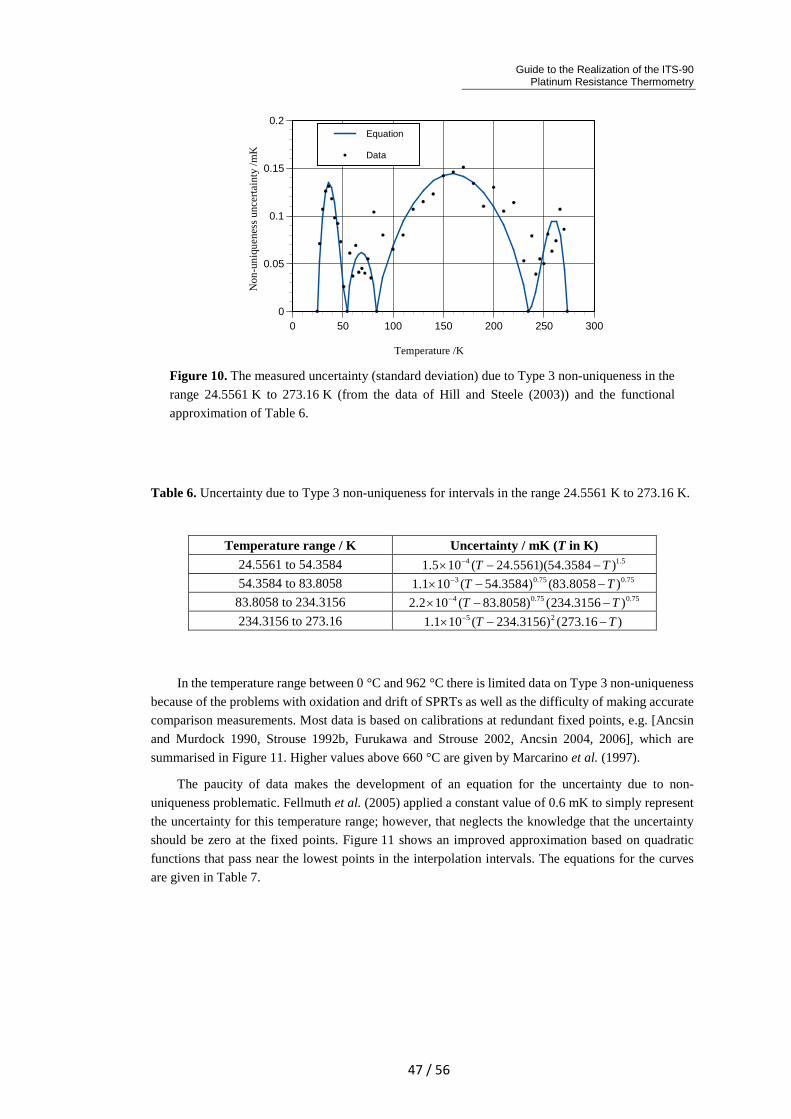
Guide to the Realization of the ITS-90 Platinum Resistance Thermometry
47 / 56
Figure 10. The measured uncertainty (standard deviation) due to Type 3 non-uniqueness in the
range 24.5561 K to 273.16 K (from the data of Hill and Steele (2003)) and the functional
approximation of Table 6.
Table 6. Uncertainty due to Type 3 non-uniqueness for intervals in the range 24.5561 K to 273.16 K.
Temperature range / K Uncertainty / mK (T in K)
24.5561 to 54.3584 4 1.51.5 10 ( 24.5561)(54.3584 )T T−× − −
54.3584 to 83.8058 3 0.75 0.751.1 10 ( 54.3584) (83.8058 )T T−× − −
83.8058 to 234.3156 4 0.75 0.752.2 10 ( 83.8058) (234.3156 )T T−× − −
234.3156 to 273.16 5 21.1 10 ( 234.3156) (273.16 )T T−× − −
In the temperature range between 0 °C and 962 °C there is limited data on Type 3 non-uniqueness
because of the problems with oxidation and drift of SPRTs as well as the difficulty of making accurate
comparison measurements. Most data is based on calibrations at redundant fixed points, e.g. [Ancsin
and Murdock 1990, Strouse 1992b, Furukawa and Strouse 2002, Ancsin 2004, 2006], which are
summarised in Figure 11. Higher values above 660 °C are given by Marcarino et al. (1997).
The paucity of data makes the development of an equation for the uncertainty due to non-
uniqueness problematic. Fellmuth et al. (2005) applied a constant value of 0.6 mK to simply represent
the uncertainty for this temperature range; however, that neglects the knowledge that the uncertainty
should be zero at the fixed points. Figure 11 shows an improved approximation based on quadratic
functions that pass near the lowest points in the interpolation intervals. The equations for the curves
are given in Table 7.
0
0.05
0.1
0.15
0.2
0 50 100 150 200 250 300
Equation
Data
Temperature /K
No
n-u
niq
uen
ess
un
cert
ain
ty /
mK
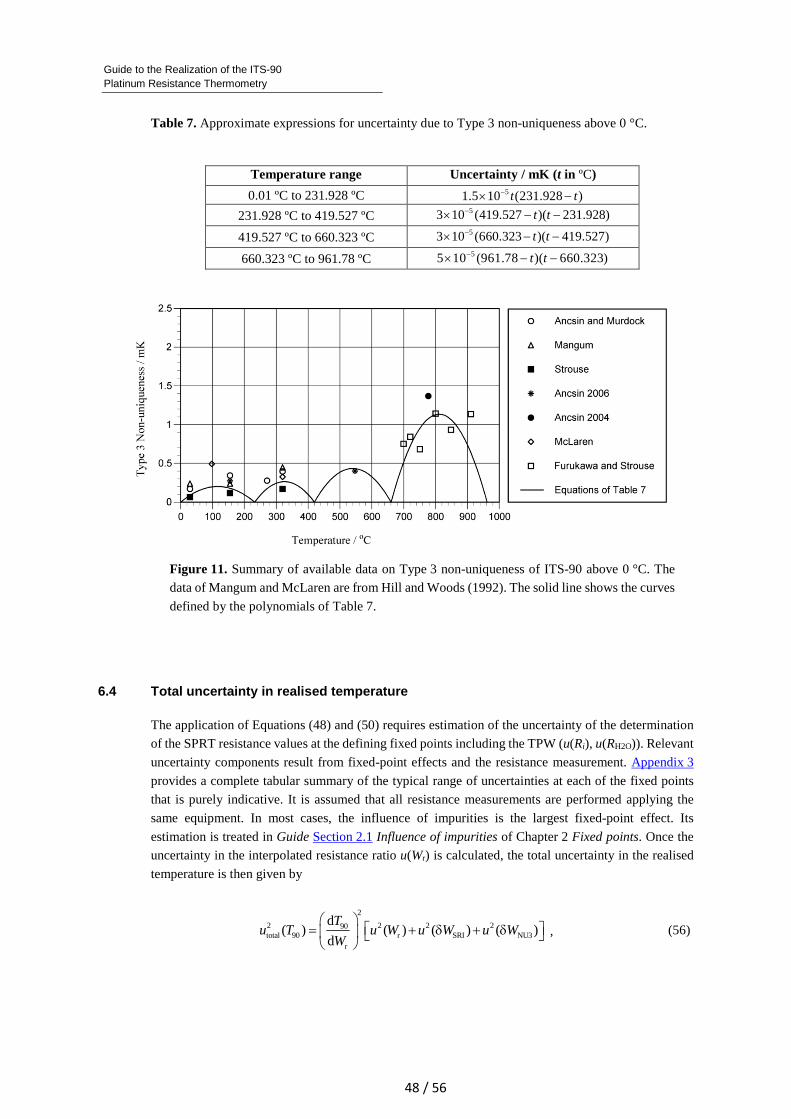
Guide to the Realization of the ITS-90
Platinum Resistance Thermometry
48 / 56
Table 7. Approximate expressions for uncertainty due to Type 3 non-uniqueness above 0 °C.
Temperature range Uncertainty / mK (t in ºC)
0.01 ºC to 231.928 ºC 51.5 10 (231.928 )t t−× −
231.928 ºC to 419.527 ºC 53 10 (419.527 )( 231.928)t t−× − −
419.527 ºC to 660.323 ºC 53 10 (660.323 )( 419.527)t t−× − −
660.323 ºC to 961.78 ºC 55 10 (961.78 )( 660.323)t t−× − −
Figure 11. Summary of available data on Type 3 non-uniqueness of ITS-90 above 0 °C. The
data of Mangum and McLaren are from Hill and Woods (1992). The solid line shows the curves
defined by the polynomials of Table 7.
6.4 Total uncertainty in realised temperature
The application of Equations (48) and (50) requires estimation of the uncertainty of the determination
of the SPRT resistance values at the defining fixed points including the TPW (u(Ri), u(RH2O)). Relevant
uncertainty components result from fixed-point effects and the resistance measurement. Appendix 3
provides a complete tabular summary of the typical range of uncertainties at each of the fixed points
that is purely indicative. It is assumed that all resistance measurements are performed applying the
same equipment. In most cases, the influence of impurities is the largest fixed-point effect. Its
estimation is treated in Guide Section 2.1 Influence of impurities of Chapter 2 Fixed points. Once the
uncertainty in the interpolated resistance ratio u(Wr) is calculated, the total uncertainty in the realised
temperature is then given by
2
2 2 2 290total 90 r SRI NU3
r
d( ) ( ) ( ) ( )
d
Tu T u W u W u W
W
= + δ + δ
, (56)
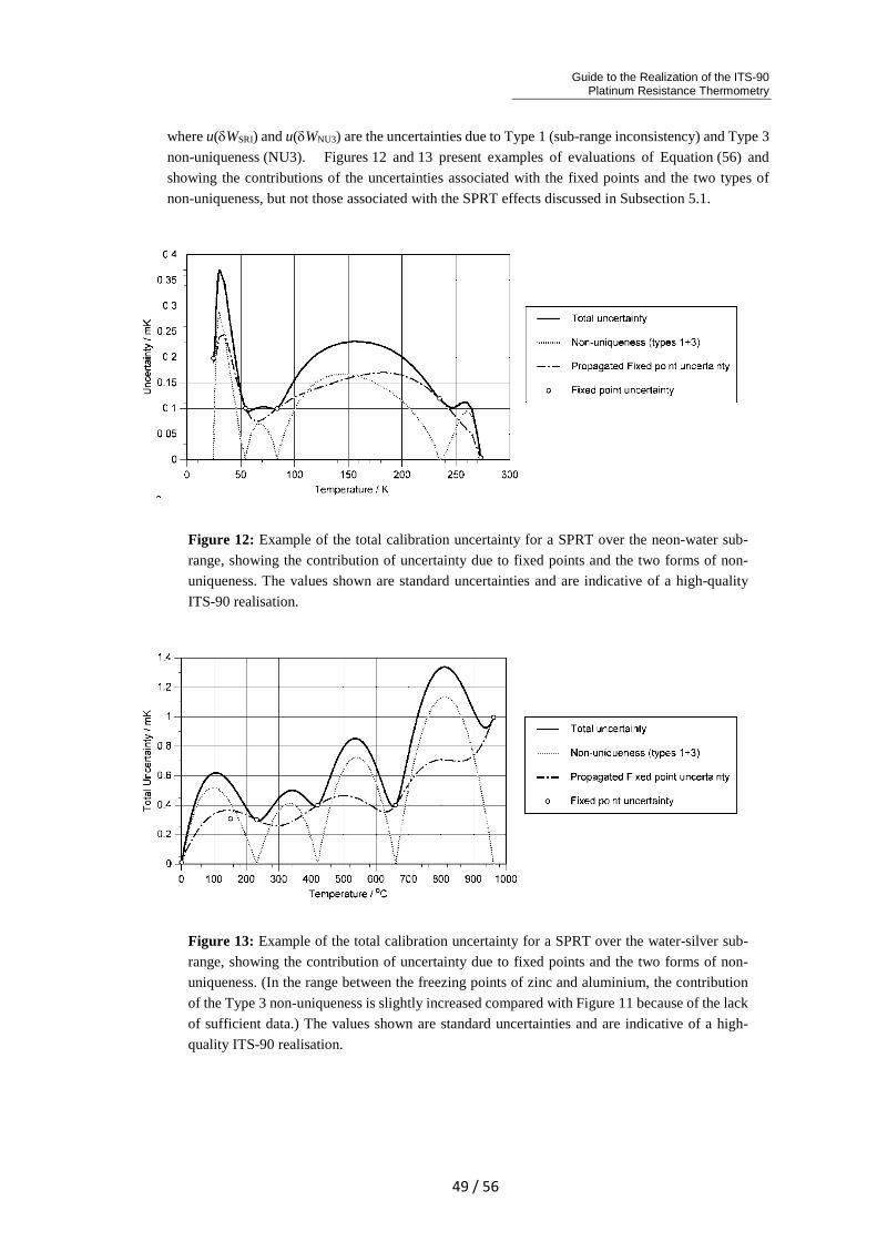
Guide to the Realization of the ITS-90 Platinum Resistance Thermometry
49 / 56
where u(δWSRI) and u(δWNU3) are the uncertainties due to Type 1 (sub-range inconsistency) and Type 3
non-uniqueness (NU3). Figures 12 and 13 present examples of evaluations of Equation (56) and
showing the contributions of the uncertainties associated with the fixed points and the two types of
non-uniqueness, but not those associated with the SPRT effects discussed in Subsection 5.1.
Figure 12: Example of the total calibration uncertainty for a SPRT over the neon-water sub-
range, showing the contribution of uncertainty due to fixed points and the two forms of non-
uniqueness. The values shown are standard uncertainties and are indicative of a high-quality
ITS-90 realisation.
Figure 13: Example of the total calibration uncertainty for a SPRT over the water-silver sub-
range, showing the contribution of uncertainty due to fixed points and the two forms of non-
uniqueness. (In the range between the freezing points of zinc and aluminium, the contribution
of the Type 3 non-uniqueness is slightly increased compared with Figure 11 because of the lack
of sufficient data.) The values shown are standard uncertainties and are indicative of a high-
quality ITS-90 realisation.
Guide to the Realization of the ITS-90
Platinum Resistance Thermometry
50 / 56
References
Ahmed M.G. 2005 Investigation of the ITS-90 sub-range inconsistencies for 25.5 Ω SPRT’s in the range 0 °C – 660 °C, Proc. 9th International Symposium on Temperature and Thermal Measurements in Industry and Science (TEMPMEKO 2004), Ed. D. Zvizdić, L.G. Bermanec, T. Veliki and T. Stašić (IMEKO / University of Zagreb, Faculty of Mechanical Engineering and Naval Architecture, Zagreb) ISBN 953-6313-71-5, pp. 271-274
Ancsin J., Murdock E.G. 1990 An intercomparison of platinum resistance thermometers between 0 °C and 630 °C, Metrologia 27, 201-209
Ancsin J. 1996 Non-uniqueness of the ITS-90, Metrologia 33, 5-17
Ancsin J. 2003 Oxidation of platinum resistance thermometers, Proc. Temperature: Its Measurement and Control in Science and Industry, Vol. 7, Ed. D. C. Ripple (AIP, New York) pp. 345-349
Ancsin J. 2004 A comparison of PRTs at the Cu-Ag eutectic point (760 °C), Metrologia 41, 198-203
Ancsin J. 2006 Non-uniqueness of ITS-90 at 548.2°C and at 156.6°C, Metrologia 43, 461-469
Awan S., Kibble B., Schurr J 2011 Coaxial electrical circuits for interference-free measurements (The Institution of Engineering and Technology, London)
Batagelj V. 2004 Thermal drain along the thermometer. Is the hydrostatic effect a relevant criteria for assuming the absence of thermal drain? CCT Workshop on Uncertainty in Temperature Fixed Points, TEMPMEKO 2004, Cavtat, Croatia, 26 June 2004, see http://www.bipm.org/cc/CCT/Allowed/23/CCT_05_01.pdf
Batagelj V., Bojkovski J., Drnovsek J. 2003a Methods of reducing the uncertainty of the self-heating correction of a standard platinum resistance thermometer in temperature measurements of the highest accuracy, Meas. Sci. Tech. 14, 2151
Batagelj V., Bojkovski J., Drnovsek J., Pusnik I. 2003b Influence of SPRT self-heating on measurement uncertainty in fixed point calibration and calibration by comparison, Proc. Temperature: Its Measurement and Control in Science and Industry, Vol. 7, Ed. D. C. Ripple (AIP, New York) pp. 315-320
Batagelj V., Bojkovski J., Drnovsek J., 2005 The numerical analyses of the temperature gradients inside the fixed-point cell, Proc. 9th International Symposium on Temperature and Thermal Measurements in Industry and Science (TEMPMEKO 2004), Ed. D. Zvizdić, L.G. Bermanec, T. Veliki and T. Stašić (IMEKO / University of Zagreb, Faculty of Mechanical Engineering and Naval Architecture, Zagreb) ISBN 953-6313-71-5, pp. 209-214
Berry R.J. 1962, The stability of platinum Resistance Thermometers at Temperatures up to 630 ºC, Proc. Temperature: Its Measurement and Control in Science and Industry, Vol 3, Ed C.M. Herzfeld (Rheinhold, New York) pp. 301-311
Berry R.J. 1963 Relationship between the real and ideal resistivity of platinum, Can. J. Phys. 41, 946-311
Berry R.J. 1966 Platinum Resistance Thermometry in the range 630 – 900 °C, Metrologia 2, 80-90
Berry R.J., Lamarche J.L.G. 1970 Departures from Matthiessen’s Rule for Vacancies in Platinum, Phys. Lett. 31A, 319-320
Berry R.J. 1972 The influence of crystal defects in platinum on platinum resistance thermometry, Proc. Temperature: Its Measurement and Control in Science and Industry, Vol 4, Ed. R.P. Hudson (ISA, Pittsburg) pp. 937-949
Berry R.J. 1978 Study of multilayer surface oxidation of platinum by electrical resistance technique, Surface Science 76, 415-442
Berry R.J. 1980 Effect of Pt Oxidation on Pt Resistance Thermometry, Metrologia 16, 117-126
Berry R.J. 1982a Evaluation and control of platinum oxidation errors in standard platinum resistance thermometers, Proc. Temperature: Its measurement and Control in Science and Industry, Vol. 5, Ed. J.F. Schooley (AIP, New York) pp. 743-752
Guide to the Realization of the ITS-90 Platinum Resistance Thermometry
51 / 56
Berry R.J. 1982b Oxidation, stability and insulation characteristics of Rosemount standard platinum resistance thermometers, Proc. Temperature: Its measurement and Control in Science and Industry, Vol. 5, Ed. J.F. Schooley (AIP, New York) pp. 743-752
Berry R.J. 1983 Thermal strain effect in standard platinum resistance thermometers, Metrologia 19, 37-47
Berry R.J. 1995 Analysis and control of electrical insulation leakage in platinum resistance thermometers up to 1064 °C, Metrologia 32, 11-25
Bonnier G., Diril A., Arai M., Ballico M., Chimenti V., Duris S., Filipe E., Ivanova A.G., Kartal Dogan A., Mendez-Lango E., Meyer C., Pavese F., Peruzzi A., Renaot E., Seidel J., Stock M., Ugur S., White D.R. 2005 Uncertainty budgets for SPRT Calibrations at the Fixed Points, Proc. 9th
International Symposium on Temperature and Thermal Measurements in Industry and Science(TEMPMEKO 2004), Ed. D. Zvizdić, L.G. Bermanec, T. Veliki and T. Stašić (IMEKO / University of Zagreb, Faculty of Mechanical Engineering and Naval Architecture, Zagreb) ISBN 953-6313-71-5, pp. 1119-1140
Evans J. P. 1984 Evaluation of some high-temperature platinum resistance thermometers, Journal of Research of the National Bureau of Standards 89, 384-373
Fahr M., Rudtsch S. 2008 A new method for the quantification and correction of thermal effects on the realization of fixed points, Int. J. Thermophys. 29, 126-138 (Proc. TEMPMEKO 2007)
Fellmuth B., Fischer J., Tegeler E. 2001 Uncertainty budgets for characteristics of SPRTs calibrated according to the ITS-90, Working Document of BIPM Consultative Committee for Thermometry, 21st Meeting, CCT/2001-02, http://www.bipm.org/cc/CCT/Allowed/21/CCT01-02.pdf.
Fellmuth B., Tegeler E., Fischer J. 2005 Uncertainty of the characteristics of SPRTs calibrated according to the ITS-90, Proc. 9th International Symposium on Temperature and Thermal Measurements in Industry and Science (TEMPMEKO 2004), Ed. D. Zvizdić, L.G. Bermanec, T. Veliki and T. Stašić (IMEKO / University of Zagreb, Faculty of Mechanical Engineering and Naval Architecture, Zagreb) ISBN 953-6313-71-5, pp. 1135-1140
Fellmuth B., Wolber L., Head D.I., Hermier Y., Hill K.D, Nakano T., Pavese F., Peruzzi A., Rusby R.L., Shkraba V., Steele A.G., Steur P.P.M., Szmyrka-Grzebyk A., Tew W.L., Wang L., White D.R. 2012 Investigation of low-temperature fixed points by an international star intercomparison of sealed triple-point cells, Metrologia 49 (3), 257-265
Fellmuth B., Fischer J., Machin G., Picard S., Steur P.P.M., Tamura O., White D.R., Yoon H. 2016 The kelvin redefinition and its mise en pratique, Phil. Trans. R. Soc. A 374, 20150037, DOI: 10.1098/rsta.2015.0037
Fischer J., Wolber L., de Podesta M., Rusby R., Hill K.D. Moldover M., Pitre L., Steur P., Tamura O., White R. 2011 Present estimates of the differences between thermodynamic temperatures and the ITS-90, Int. J. Thermophys. 32, 12-25 (Proc. of TEMPMEKO 2010).
Furukawa G.T., Strouse G.F. 2002 Investigation of the non-uniqueness of the ITS-90 in the range 660 °C to 962 °C, Proc. 8th International Symposium on Temperature and Thermal Measurements in Industry and Science (TEMPMEKO 2001), Ed. Fellmuth B., Seidel J., Scholz G. (VDE Verlag, Berlin) ISBN 3-8007-2676-9, pp. 553-558
Gaiţă S., Iliescu C. 2001 Propagation of combined standard uncertainties evaluated in SPRT calibration according to ITS-90, Proc. of the International Conference of Metrology, Bucharest, Romania (ISBN 973-99385-5-8), http://www.temperature.ro/Arhiva/Propagation of combined standard uncertainties evaluated in SPRT calibration according to ITS-90.pdf
Gaiser C., Fellmuth B. 2013a Temperature-measurement errors with capsule-type resistance thermometers, Proc. Temperature: Its Measurement and Control in Science and Industry, Vol. 8, Ed. C.W. Meyer (American Institute of Physics, Melville, New York) AIP Conference Proceedings Vol. 1552, ISBN 978-0-7354-1178-4, pp. 427-432
Guide to the Realization of the ITS-90
Platinum Resistance Thermometry
52 / 56
Gaiser C., Fellmuth B. 2013b Static thermal measurement errors using resistance thermometers, Proc. Temperatur 2013, Fachtagung Berlin, 5./6.6.2013 (Physikalisch-Technische Bundesanstalt, Berlin) ISBN 3-9810021-8-0, pp. 85-90
Head D. I. 1997 A EUROMET intercomparison of capsule platinum resistance thermometers between 13 K and 273 K, Proc. of the International Seminar on Low Temperature Thermometry and Dynamic Temperature Measurement, Ed. A. Szmyrka-Grzebyk (IMEKO, DRUK, Wrocław) pp. L36 – L41
Hill K.D., Steele A.G. 2003 The non-uniqueness of the ITS-90: 13.8033 K to 273.16 K, Proc. Temperature: Its Measurement and Control in Science and Industry, Vol. 7, Ed. D. C. Ripple (AIP, New York) pp. 53-58
Hill K.D., Woods D.J. 1992 A preliminary assessment of the non-uniqueness of the ITS-90 in the range 500 ºC to 660 ºC as measured with a caesium-filled pressure-controlled, heat-pipe furnace, Proc. Temperature, Its Measurement and Control in Science and Industry, Vol. 6, Ed. J.F Schooley (AIP, New York) pp. 215-219
Hill K.D. 2015 High-temperature platinum resistance thermometry: the problem with silver and the case for gold, Metrologia 52, 478-485
Hill K.D. 1995 Inconsistency in the ITS-90 and the triple point of mercury, Metrologia 32, 87-94
Hust J. 1970 Rev. Sci. Instr. 41, 622-624
Ilin A.U. 2003 A Criterion for Uniformity of a Temperature Field in Realization of the ITS-90 Fixed Points, Proc. Temperature: Its Measurement and Control in Science and Industry, Vol. 7, Ed. D. C. Ripple (AIP, New York) pp. 297-301
Ivanova A.G., Ilin A.U. 2005 Influence of the realising method on the freezing temperature of zinc, Izmeritelnaja Technika 11, 43-46 (Presented to TEMPMEKO 2004, Translation: Measurement Techniques 47, 1096-1099)
Ivanova A.G., Abasov M.Y., Gerasimov S.F., Pokhodun A.I. 2013 Measurement of the In Freezing-Point Temperature: Effect of the Liquid-Solid Interface Structure, Proc. Temperature: Its Measurement and Control in Science and Industry, Vol. 8, Ed. C.W. Meyer (American Institute of Physics, Melville, New York) AIP Conference Proceedings Vol. 1552, ISBN 978-0-7354-1178-4, pp. 243-248
Jursic I., Rudtsch S. 2014 Thermal Stability of β-PtO2 Investigated by Simultaneous Thermal Analysis and Its Influence on Platinum Resistance Thermometry, Int. J. Thermophys. 35, 1055–1066
Kemp R.C., Kemp W.R.G., Cowan J.A. 1976 The Boiling Points and Triple Points of Oxygen and Argon, Metrologia 12, 93-100
Kemp R.C. 1991 The Reference Function for Platinum Resistance Thermometer Interpolation between 13,8033 K and 273,16 K in the International Temperature Scale of 1990, Metrologia 28, 327-332
Kirby C.G.M., Laubitz M.J. 1973 The Error Due to the Peltier Effect in Direct-Current Measurements of Resistance, Metrologia 9, 103-106
Mangum B.W., Pfeiffer E.R., Strouse G.F. 1990 Non-uniqueness of some standard platinum resistance thermometers over the temperature range from 13 K to 1235 K, Proc. 4th Symposium on Temperature and Thermal Measurements in Industry and Science (TEMPMEKO 1990) (Finnish Society of Automatic Control, Helsinki) ISBN 9789519604220, pp 17-36
Mangum B.W., Bloembergen P., Chattle M.V., Fellmuth B., Marcarino P., Pokhodun A.I. 1997 On the International Temperature Scale of 1990 (ITS-90), Metrologia 34, 427-429
Mangum B.W., Bloembergen P., Chattle M.V., Fellmuth B., Marcarino P., Pokhodun A.I. 1999 On the International Temperature Scale of 1990 (ITS-90). Part II: Recommended techniques for comparisons, at the highest level of accuracy, of fixed-point cells used for contact thermometry, Metrologia 36, 79-88
Mangum B.W., Bloembergen P., Chattle M.V., Fellmuth B., Marcarino P., Pokhodun A.I. 2000 Optimal realization of the defining points of the ITS-90 that are used in contact thermometry,
Guide to the Realization of the ITS-90 Platinum Resistance Thermometry
53 / 56
Working Document of BIPM Consultative Committee for Thermometry, 20th Meeting, Document CCT/2000-13 (This document is available on request from the BIPM.)
Mangum B.W., Strouse G.F. Guthrie W.F., Pello R., Stock M., Renaot E., Hermier Y., Bonnier G., Marcarino P, Gam K.S., Kang K.H., Kim Y.-G., Nicholas V., White D.R., Dransfield T.D., Duan Y., Qu Y., Connolly J., Rusby R.L., Gray J., Sutton G.J.M., Head D.I., Hill, K.D., Steele, A., Nara K., Tegeler E., Noatsch U., Heyer D., Fellmuth B., Thiele-Krivoy B., Duris S., Pokhodun A.I., Moiseeva N.P., Ivanova A.G., de Groot M.J., Dubbeldam J.F. 2002 Summary of comparison of realizations of the ITS-90 over the range 83.8058 K to 933.473 K: CCT Key Comparison CCT-K3, Metrologia 39, 179-205
Marcarino P., Dematteis R., Gallorini M., and Rizzio E. 1989 Contamination of Platinum Resistance Thermometers at High Temperature Through Their Silica Sheaths, Metrologia 26, 175-181
Marcarino P., Dematteis R., Li X., Arai M., de Groot M., Nubbemeyer H.G. 1997 Preliminary results on ITS-90 non-uniqueness between freezing points of Al and Ag, Proc. 6th International Symposium on Temperature and Thermal Measurements in Industry and Science (TEMPMEKO 1996), Ed. P. Marcarino (Levrotto & Bella, Torino) pp. 25-32
Marcarino P., Steur P.P.M., Dematteis R. 1999 Calibration of SPRTs, affected by humidity, in the sub-range between the fixed points of Hg and Ga, Proc. 7th International Symposium on Temperature and Thermal Measurements in Industry and Science (TEMPMEKO ’99), Ed. J.F. Dubbeldam, M.J. de Groot (IMEKO / NMi Van Swinden Laboratorium, Delft) pp. 80-83
McLaren E.H. and Murdock E.G. 1966 Radiation Effects in Precision Resistance Thermometry. II. Illumination Effect on Temperature Measurement in Water Triple-point Cells Packed in Crushed Ice, Canadian Journal of Physics 44, 2653-2659
McMartin M. P., Kusters N.L. 1966 A Direct-Current-Comparator Ratio Bridge for Four-Terminal Resistance Measurements, IEEE Tans. Instrum. Meas. IM-15, 212-220
Meyer C. W., Ripple D.C. 2006 Determination of the uncertainties for ITS-90 realization by SPRTs between fixed points, Metrologia 43, 327-340
Meyer C.W., Tew W.L. 2006 ITS-90 non-uniqueness from PRT sub-range inconsistencies over the range 24.56 K to 273.16 K, Metrologia 43, 341-352
Moiseeva N.P., Pokhodun A.I. 1992 Investigation of the non-uniqueness and sub-range inconsistency of ITS-90 using platinum resistance thermometers in the 0-961.78 °C range, Proc. Temperature: Its Measurement and Control in Science and Industry, Vol. 6, Ed. J. F. Schooley (Am. Inst. of Phys., New York) pp. 187-191
Moiseeva N.P. 2005 Improved design for 0.6-ohm HTSPRTS: reducing the leakage error and increasing the stability. Proc. 9th International Symposium on Temperature and Thermal Measurements in Industry and Science (TEMPMEKO 2004), Ed. D. Zvizdić, L.G. Bermanec, T. Veliki and T. Stašić (IMEKO / University of Zagreb, Faculty of Mechanical Engineering and Naval Architecture, Zagreb) ISBN 953-6313-71-5, pp. 433-438
Nubbemeyer H.G., Fischer J. 2002 Final report on key comparison CCT-K4 of local realizations of aluminium and silver freezing-point temperatures, Metrologia 39, Tech. Suppl., 03001
Pavese F., Ancsin J., Astrov D.N., Bonhoure J., Bonnier G., Furukawa G.T., Kemp R.C., Maas H., Rusby R.L., Sakurai H., Ling Shan-Kang 1984 An International Intercomparison of Fixed Points by Means of Sealed Cells in the Range 13.81 K - 90.686 K, Metrologia 20, 127-144
Pearce J.V., Harris P.M., Rusby R.L., Wright L. 2013 The optimization of self-heating corrections in resistance thermometry, Metrologia 50, 345-353
Pearce J.V., Rusby R.L., Harris P.M., Wright L. 2012 Optimising the extrapolation to zero current in SPRT self-heating corrections, Working Document of BIPM Consultative Committee for Thermometry, 26th Meeting, Document CCT/12-16 (This document is available on request from the BIPM.)
Pokhodun A.I. 2002 Investigation of some factors influencing the stability of standard platinum resistance thermometers in the interval above 273,16 K, Proc. 8th International Symposium on
Guide to the Realization of the ITS-90
Platinum Resistance Thermometry
54 / 56
Temperature and Thermal Measurements in Industry and Science (TEMPMEKO 2001), Ed. Fellmuth B., Seidel J., Scholz G. (VDE Verlag, Berlin) ISBN 3-8007-2676-9, pp. 97-102
Pokhodun A.I., Moiseyeva N.P., Kovalev A.V., Khovanskaya E.V. 1990 Investigation of the Metrological Characteristics of Soviet-made High-Temperature Platinum Resistance Thermometers, Proc. 4th Symposium on Temperature and Thermal Measurements in Industry and Science (TEMPMEKO 1990) (Finnish Society of Automatic Control, Helsinki) ISBN9789519604220, pp 37-53
Pokhodun A.I., Renaot E., Bonnier G., Studenok E. 2005 Study into the Effect of the Platinum Wire Quality upon the Instability of HTPRT, Proc. 9th International Symposium on Temperature and Thermal Measurements in Industry and Science (TEMPMEKO 2004), Ed. D. Zvizdić, L.G. Bermanec, T. Veliki and T. Stašić (IMEKO / University of Zagreb, Faculty of Mechanical Engineering and Naval Architecture, Zagreb) ISBN 953-6313-71-5, pp. 439-444
Renaot E., Valin M.H., Bonnier G., White M., Van der Linden A., Bairy G., Kovacs T., Nemeth S., Bojkovski J., Kuna R., Weckstrom T., Ivarsson J., Rauta C., Helgesen F., Uytun A., Ugur S., Kryl J., Adunka F., Ranostaj J., Duris S., Anagnostou M., Kokkini E., Pauza A., Augevicius V. 2005 Comparison of realisations of the triple point of water (EUROMET project No. 549), Proc. 9th International Symposium on Temperature and Thermal Measurements in Industry and Science (TEMPMEKO 2004), Ed. D. Zvizdić, L.G. Bermanec, T. Veliki and T. Stašić (IMEKO / University of Zagreb, Faculty of Mechanical Engineering and Naval Architecture, Zagreb) ISBN 953-6313-71-5, pp. 1009-1015
Riddle J.L., Furukawa, G.T., Plumb, H.H. 1973 Platinum Resistance Thermometry, NBS Monograph 126 (National Bureau of Standards, Washington) April 1973
Ripple D. C., Davis R., Fellmuth B., Fischer J., Machin G., Quinn T., Steur P., Tamura O., White D.R. 2010 The Roles of the Mise en Pratique for the Definition of the Kelvin, Int. J. Thermophys. 31, 1795–1808
Rudtsch S., Ramm G., Heyer D., Vollmert R. 2005 Comparison of Test and Calibration Methods for Resistance Ratio Bridges, Proc. 9th International Symposium on Temperature and Thermal Measurements in Industry and Science (TEMPMEKO 2004), Ed. D. Zvizdić, L.G. Bermanec, T. Veliki and T. Stašić (IMEKO / University of Zagreb, Faculty of Mechanical Engineering and Naval Architecture, Zagreb) ISBN 953-6313-71-5, pp. 773-780
Rusby R.L. 1993, The mercury point in the ITS-90, Working Document of BIPM Consultative Committee for Thermometry, 18th Meeting, Document CCT/93-29 (This document is available on request from the BIPM.)
Rusby R.L. 2010 The discontinuity in the first derivative of the ITS-90 at the triple point of water, Int. J. Thermophys. 31, 1567-1572 (Proc. TEMPMEKO 2010)
Rusby R.L., Pearce J.V., Elliott C.J. 2017 Considerations Relating to Type 1 and Type 3 Non-uniqueness in SPRT Interpolations of the ITS-90, Int. J. Thermophys. 38, 186 (Proc. TEMPMEKO 2016), DOI 10.1007/s10765-017-2319-2
Sakurai H., Tamura O. 2011 Oxidization Characteristics of Standard Platinum Resistance Thermometers, Jpn. J. Appl. Phys. 50, 036601-1-036601-7, DOI: 10.1143/JJAP.50.036601
Sakurai H., Yamaguchi T., Hiura N., Yoneshita K., Kimura H., Tamura O. 2008 Oxidization Characteristics of Some Standard Platinum Resistance Thermometers, Jpn. J. Appl. Phys. 47, 8071-8076
Seriani N., Pompe W. Colombi Ciacchi L. 2006 Catalytic Oxidation Activity of Pt3O4 Surfaces and Thin Films, J. Phys. Chem. B 110 (30), 14860–14869
Singh Y.P., Maas H., Edler F., Zaidi Z.H. 1994 Correlation between the resistance ratios of platinum resistance thermometers at the melting point of gallium and the triple point of mercury, Metrologia 31, 49-50
Steele A.G. 2005 ITS-90 Sub-range inconsistency below the triple point of water, Metrologia 42, 289-297
Guide to the Realization of the ITS-90 Platinum Resistance Thermometry
55 / 56
Steele A.G., Fellmuth B., Head D.I., Hermier Y., Kang K.H., Steur P.P.M., Tew W.L. 2002 Key Comparison: CCT-K2: Key comparison of capsule-type standard platinum resistance thermometers from 13.8 K to 273.16 K, Metrologia 39, 551-571
Stock M., Solve S. 2005 Report on CCT-K7, Key comparison of water triple point cells, Draft B-2, 22 August 2005, rev.1 (available at www.bipm.fr)
Stock M. et al. 2006 Final Report on CCT-K7: Key comparison of water triple point cells, Metrologia43, Tech. Suppl. 03001
Strouse G.F 1992a Investigation of the ITS-90 sub-range inconsistencies for 25.5 Ω SPRTs, Proc. Temperature: Its Measurement and Control in Science and Industry, Vol. 6, Ed. J.F Schooley (AIP, New York) pp. 165-168
Strouse G.F. 1992b NIST assessment of ITS-90 non-uniqueness for 25.5 Ω SPRTs at gallium, indium and cadmium fixed points, Proc. Temperature: Its Measurement and Control in Science and Industry, Vol. 6, Ed. J.F Schooley (AIP, New York) pp. 175-178
Strouse G.F. 2005 NIST certification of ITS-90 Fixed-point cells from 83.8058 K to 1234.93 K: Methods and Uncertainties, Proc. 9th International Symposium on Temperature and Thermal Measurements in Industry and Science (TEMPMEKO 2004), Ed. D. Zvizdić, L.G. Bermanec, T. Veliki and T. Stašić (IMEKO / University of Zagreb, Faculty of Mechanical Engineering and Naval Architecture, Zagreb) ISBN 953-6313-71-5, pp. 879-884
Strouse G.F., Hill K.D. 2003 Performance Assessment of resistance Ratio Bridges Used for the Calibration of SPRTs, Proc. Temperature: Its Measurement and Control in Science and Industry, Vol. 7, Ed. D. C. Ripple (AIP, New York) pp. 327-332
Tew W. L., Murdock W. E., Chojnacky M. J., Ripple D. C. 2013 The residual and temperature-dependent resistance of reference-grade platinum wire below 13.8 K, Proc. Temperature: Its Measurement and Control in Science and Industry, Vol. 8, Ed. C.W. Meyer (American Institute of Physics, Melville, New York) AIP Conference Proceedings Vol. 1552, ISBN 978-0-7354-1178-4, pp. 457-462
Ward S.D., Compton J.P. 1979 Intercomparison of Platinum Resistance Thermometers and T68
Calibrations, Metrologia 15, 31-46
Wang C., Yeh C. 1998 Effects of particle size on the progressive oxidation of nanometer platinum by dioxygen, J. Catal. 178, 450-456
White D.R. 1997 A Method for Calibrating Resistance Thermometry Bridges, Proc. 6th International Symposium on Temperature and Thermal Measurements in Industry and Science (TEMPMEKO 1996), Ed. P. Marcarino (Levrotto & Bella, Torino) pp. 129-134
White D.R. 2003 Contribution of Uncertainties in Resistance Measurements to Uncertainty in ITS-90, Proc. Temperature: Its Measurement and Control in Science and Industry, Vol. 7, Ed. D.C. Ripple (AIP, New York) pp. 321-326
White D.R., Saunders P. 2007 The propagation of uncertainty with calibration equations, Meas. Sci. Technol. 18, 2157-2169
White D.R., Arai M., Bittar A., Yamazawa K. 2007 A Schottky-Diode Model of Insulation Resistance Effects in SPRTS - Part 1, Int. J. Thermophys. 28, 1843-1854
White D.R., Strouse G.F. 2009 Observations on sub-range inconsistency in the SPRT interpolations of ITS-90, Metrologia 46, 101–108
White D.R., Jongenelen A. 2010 The immersion characteristics of industrial PRTs, Int. J. Thermophys. 31, 1685–95
White D.R., Mason R.S. 2011 Improved Initiation Technique for the Metal Fixed Points, Int. J. Thermophys. 32, 348-359
White D.R. 2013 Some Mathematical Properties Of The ITS-90, Proc. Temperature: Its Measurement and Control in Science and Industry, Vol. 8, Ed. C.W. Meyer (American Institute of Physics, Melville, New York) AIP Conference Proceedings Vol. 1552, ISBN 978-0-7354-1178-4, pp. 81-88
Guide to the Realization of the ITS-90
Platinum Resistance Thermometry
56 / 56
White D.R., Edgar H. 2013 Optimizing the Resolution of Resistance Bridges, Proc. Temperature: Its Measurement and Control in Science and Industry, Vol. 8, Ed. C.W. Meyer (American Institute of Physics, Melville, New York) AIP Conference Proceedings Vol. 1552, ISBN 978-0-7354-1178-4, pp. 398-403
White D.R. et al. 2018 to be published in Metrologia
Widiatmo J.V., Harada K., Yamazawa K., Arai M. 2006 Estimation of impurity effect in aluminium fixed-point cells based on thermal analysis, Metrologia 43, 561
Widiatmo J.V., Harada K., Yamazawa K., Arai M. 2013 Electrical Effects in Measurements at the Silver Point using High Temperature SPRTs, Proc. Temperature: Its Measurement and Control in Science and Industry, Vol. 8, Ed. C.W. Meyer (American Institute of Physics, Melville, New York) AIP Conference Proceedings Vol. 1552, ISBN 978-0-7354-1178-4, pp. 271-276
Wilkins F.J., Swan M.J. 1970 Precision ac/dc resistance standards, Proc. IEE 117, 841-849
Yamazawa K., Arai M. 2003 Measurement of the insulation resistance for the development of high temperature platinum resistance thermometers with a guard electrode, Proc. Temperature: Its Measurement and Control in Science and Industry, Vol. 7, Ed. D. C. Ripple (AIP, New York) pp. 363-368
Yamazawa K., Arai M. 2005 Design improvement against the lead leakage effect for high temperature SPRTs up to 1085 °C, Proc. 9th International Symposium on Temperature and Thermal Measurements in Industry and Science (TEMPMEKO 2004), Ed. D. Zvizdić, L.G. Bermanec, T. Veliki and T. Stašić (IMEKO / University of Zagreb, Faculty of Mechanical Engineering and Naval Architecture, Zagreb) ISBN 953-6313-71-5, pp. 409-414
Yamazawa K., Arai M., White D.R. 2007 A Schottky-Diode Model of Insulation Resistance Effects in SPRTS - Part 2, Int. J. Thermophys. 28, 1855-1867
Zhang J., Berry R.J. 1985 Ac and Dc Insulation Leakage in platinum Resistance Thermometers up to 750 ºC, Metrologia 21, 207-223
Zhiru K., Jingbo L., Xiaoting L. 2002 Study of the ITS-90 non-uniqueness for the standard platinum resistance thermometer in the sub-range 0 °C to 419.527 °C, Metrologia 39, 127-133
Žužek V., Batagelj V., Drnovšek J., Bojkovski J. 2014 Open Zinc Freezing-Point Cell Assembly and Evaluation, Int. J. Thermophys. 35, 1147-1155
APPENDICES
Appendix 1 Alternative interpolating functions for special applications
Appendix 2 Typical resistance ratios and sensitivity factors for SPRTs in the ITS-90, as
well as the propagation of uncertainty from the triple point of water
Appendix 3 Summary of typical ranges of Type B standard uncertainties of the calibration
of SPRTs at the fixed points