Embed Size (px)
Citation preview
i
GUI Signal Analysis and Filtering Design
Axel Daniela Campero Vega, Electrical Engineering
Project Advisor: Dr. Dick Blandford
April 26, 2018 Evansville, Indiana

ii
Acknowledgements
I want to thank Dr. Blandford for his guidance, advice, collaboration and patience that
have allowed me to successfully completed this project. I also want to thank Dr. Howe
for her support and guidance in the preparation of this document.

iii
Table of Contents
I. Introduction
II. Problem Definition
Finite Impulse Response Filter (FIR)
Minimum requirements
III. Solution (Design)
3.1 FIR FILTERS
3.1.1 GUI DESIGN
3.1.2 Functions
a) Reset function
b) Preset function
c) Parameter setting function
d) Memory function
e) Test with an audio signal
3.1.3 Program Description
a) Filter analysis program:
b) Program of change of parameters
c) Memory and loading program
3.2 IIR FILTERS
3.2.1 GUI DESIGN
3.2.2 Functions
a) Preset function
b) Setting function
c) Visualizing Poles and zeros function
d) Execute or leave function
e) Modify Pole and zeros function
f) Insert Poles or Zeros Function
g) Reset Function
3.2.3 Program Description
a) Filter analysis program:

iv
Safety Designing Filters
IV. Costs
V. Conclusions
Appendix A: Code for FIR Filters Analysis
References
List of figures
Fig. 1 Specification of the filter
Fig. 2: Design techniques
Fig. 3 Design
Fig. 4 GUI Screen for FIR Filters
Fig. 5 Functional Block Diagram of the project
Fig. 6 Results from Reset function
Fig. 7 Results from Preset function
Fig. 8 Parameter setting function
Fig. 9 Memory and recall functions
Fig 10 Test with an audio signal
Fig. 11 Software Block Diagram
Fig. 12 Flux Diagram of the Project
Fig. 13 GUI Screen example of results for FIR Filters
Fig. 14 GUI Screen for IIR Filters
Fig. 15 IIR functions
Fig. 16 Preset function for IIR Filters
Fig. 17 Software Block Diagram for IIR Filters
Fig. 18 GUI Screen example of results for IIR Filters
List of tables
Table 1. Cost of the project
1
I. Introduction
A digital filter operates by applying mathematics to an input signal and modifies
it to produce an output that we desire. Traditionally, they are used in:
• Separation of signals to be transmitted by shared means such as cellular telephony
• Recovering distorted signals
• Sound synthesis
• Audio effects: like chorus, reverb, and so on
• Instrumentation
• Image processing
• Seismic and geophysical signal processing
• Biological signal processing and electro medicine
• Synthesis and speech recognition
• Astronomy
Traditional digital filters applications generate millionaire profits by new products
and services, and there are many industries involved. In addition, digital filters are being
applied in the financial and business area to solve problems such as; trading strategies,
trading costs, industrial processes optimization, risk prediction and other type of analysis
in order to improve business and industries. Therefore, the development of an application
about digital filters is very useful and important. This project focused on designing a
graphic user interface (GUI) application in Matlab that is capable of assisting in signal
analysis and optimization of finite impulse response (FIR) filtering.
II. Problem Definition
The design of digital filters and their influence on filtered signals are time-
consuming and a complicated process. There are tools in Matlab that help to simplify the
problem. However, there is no tool that is able to graphically modify the behavior of the
filter in relation to a previously defined ideal filter, adjust it manually or automatically
and save the results in memory.
2
The current technological requirement includes sophisticated and critical
applications in design and use of filters. For example, cellular telephony, which has
limited and small bandwidth requires the reuse of frequencies to provide service. In
addition, these filters must be dynamic, since they must adapt to the conditions of the
service area and the technology offered by the operator (GPRS, EDGE, LTE, OFDM, and
so on) [4]. These filters, are of such high order that it is not feasible to attempt their
design without the support of a mathematical tool that helps to perform the required
calculations. An actual implementation of a digital filter can start with the design of the
filter in Matlab and after finding the parameters, they are programmed into a micro
controller for their physical incorporation into the devices.
Matlab has developed an extensive library of functions that help in the design of
filters. These functions include the calculation of filter parameters, and its Bode plot in
magnitude and phase. It also includes the function diagram of poles and zeros. The source
codes for these functions are not accessible or modifiable. When a design is required, the
designer should often use the default functions in Matlab (trial and error) several times,
resulting in waste of time and low efficiency. Matlab has also developed applications of
the "toolbox" type, which help in the study of the signals subjected to filters in a more
elaborate and consumption-oriented way before the design and implementation of filters.
Moreover, these applications developed by Matlab, are not incorporated in the general
license of use of Matlab and are sold separately.
The problem can be summarized, as there is no tool or application developed in
Matlab that helps in the design and study of the dynamic behavior of the filters.
Finite Impulse Response Filter (FIR)
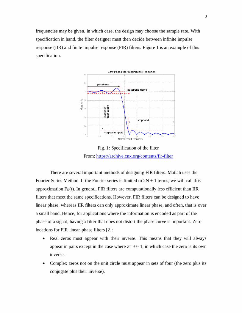
The design of a digital filter [2] typically begins with a frequency specification.
For example, a specification for a low pass filter might give a passband range as being 0
Hz to 200 Hz and a stopband as being 2254 Hz to half the sample frequency. The
specification would also indicate the amount of ripple that is permitted in the passbands
and stopband. In addition, a sample rate might be specified, or some range of sample
3
frequencies may be given, in which case, the design may choose the sample rate. With
specification in hand, the filter designer must then decide between infinite impulse
response (IIR) and finite impulse response (FIR) filters. Figure 1 is an example of this
specification.
Fig. 1: Specification of the filter
From: https://archive.cnx.org/contents/fir-filter
There are several important methods of designing FIR filters. Matlab uses the
Fourier Series Method. If the Fourier series is limited to 2N + 1 terms, we will call this
approximation FN(t). In general, FIR filters are computationally less efficient than IIR
filters that meet the same specifications. However, FIR filters can be designed to have
linear phase, whereas IIR filters can only approximate linear phase, and often, that is over
a small band. Hence, for applications where the information is encoded as part of the
phase of a signal, having a filter that does not distort the phase curve is important. Zero
locations for FIR linear-phase filters [2]:
Real zeros must appear with their inverse. This means that they will always
appear in pairs except in the case where z= +/- 1, in which case the zero is its own
inverse.
Complex zeros not on the unit circle must appear in sets of four (the zero plus its
conjugate plus their inverse).

4
Complex zeros on the unit circle must appear as conjugate pairs. In this case, the
conjugate (z) = inverse (z).
Minimum requirements:
The project will be developed in a GUI environment in Matlab language in a
flexible way, easy to handle and that will serve as a tool to support in order to
analyze FIR filters.
Selection of the filter parameters of a menu from the GUI application.
Presentation of the Bode and of the poles and zeros diagram.
Online modification of the parameters and the graphics of the filter.
Memorization of the states achieved in the filter settings.
Automatic adjustment of parameters using the minimum error principle with
reference to an ideal filter defined from the application itself.
III. Solution (Design)
The design starts with the development of the GUI (graphic user interface) screen,
defining two areas of graphics, dynamics where the results will be presented either for the
Bode and Z-Plane diagrams and their frequency spectrum. Dynamic controls are also
incorporated as a slider that serve as a dynamic control of the values that the parameters
of the transfer function can assume.
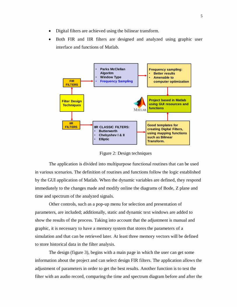
The design techniques for FIR filters are:
Parks McClellan,
Window type and
Frequency Sampling.
I choose Frequency Sampling because has better results, and it is amenable for computer
optimization. For the IIR filters the analysis use the classical Chebyshev, Butterworth and
Elliptic.
5
Digital filters are achieved using the bilinear transform.
Both FIR and IIR filters are designed and analyzed using graphic user
interface and functions of Matlab.
Filter Design
Techniques
• Parks McClellan
Algoritm
• Window Type
• Frequency Sampling
Frequency sampling:
• Better results
• Amenable to
computer optimizationFIR
FILTERS
IIR
FILTERS IIR CLASSIC FILTERS:
• Butterworth
• Chebyshev I & II
• Elliptic
Good templates for
creating Digital Filters,
using mapping functions
such as Bilinear
Transform.
Project based in Matlab
using GUI resources and
functions
Figure 2: Design techniques
The application is divided into multipurpose functional routines that can be used
in various scenarios. The definition of routines and functions follow the logic established
by the GUI application of Matlab. When the dynamic variables are defined, they respond
immediately to the changes made and modify online the diagrams of Bode, Z plane and
time and spectrum of the analyzed signals.
Other controls, such as a pop-up menu for selection and presentation of
parameters, are included; additionally, static and dynamic text windows are added to
show the results of the process. Taking into account that the adjustment is manual and
graphic, it is necessary to have a memory system that stores the parameters of a
simulation and that can be retrieved later. At least three memory vectors will be defined
to store historical data in the filter analysis.
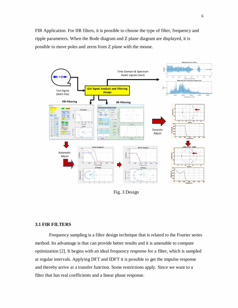
The design (figure 3), begins with a main page in which the user can get some
information about the project and can select design FIR filters. The application allows the
adjustment of parameters in order to get the best results. Another function is to test the
filter with an audio record, comparing the time and spectrum diagram before and after the
6
FIR Application. For IIR filters, it is possible to choose the type of filter, frequency and
ripple parameters. When the Bode diagram and Z plane diagram are displayed, it is
possible to move poles and zeros from Z plane with the mouse.
GUI Signal Analysis and Filtering Design
Test Signal(WAV File)
Time Domain & SpectrumAudio signals (test)
IIR Filtering
Dynamic Adjust
FIR Filtering
AutomaticAdjust
Fig. 3 Design
3.1 FIR FILTERS
Frequency sampling is a filter design technique that is related to the Fourier series
method. Its advantage is that can provide better results and it is amenable to compute
optimization [2]. It begins with an ideal frequency response for a filter, which is sampled
at regular intervals. Applying DFT and IDFT it is possible to get the impulse response
and thereby arrive at a transfer function. Some restrictions apply. Since we want to a
filter that has real coefficients and a linear phase response.
7
3.1.1 GUI DESIGN
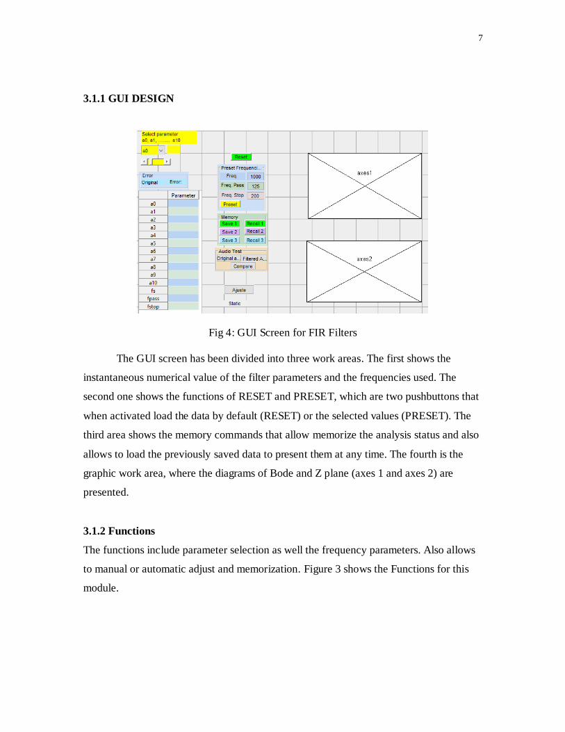
Fig 4: GUI Screen for FIR Filters
The GUI screen has been divided into three work areas. The first shows the
instantaneous numerical value of the filter parameters and the frequencies used. The
second one shows the functions of RESET and PRESET, which are two pushbuttons that
when activated load the data by default (RESET) or the selected values (PRESET). The
third area shows the memory commands that allow memorize the analysis status and also
allows to load the previously saved data to present them at any time. The fourth is the
graphic work area, where the diagrams of Bode and Z plane (axes 1 and axes 2) are
presented.
3.1.2 Functions
The functions include parameter selection as well the frequency parameters. Also allows
to manual or automatic adjust and memorization. Figure 3 shows the Functions for this
module.
8
GUI Filter Design
FIR filter
Parameter selection
a0, a1,…. anfs, fstop, fpass
Memory
Reload from
memory
Automatic
AdjustReset
Manual
Adjust
Test with an
audio signaland compare
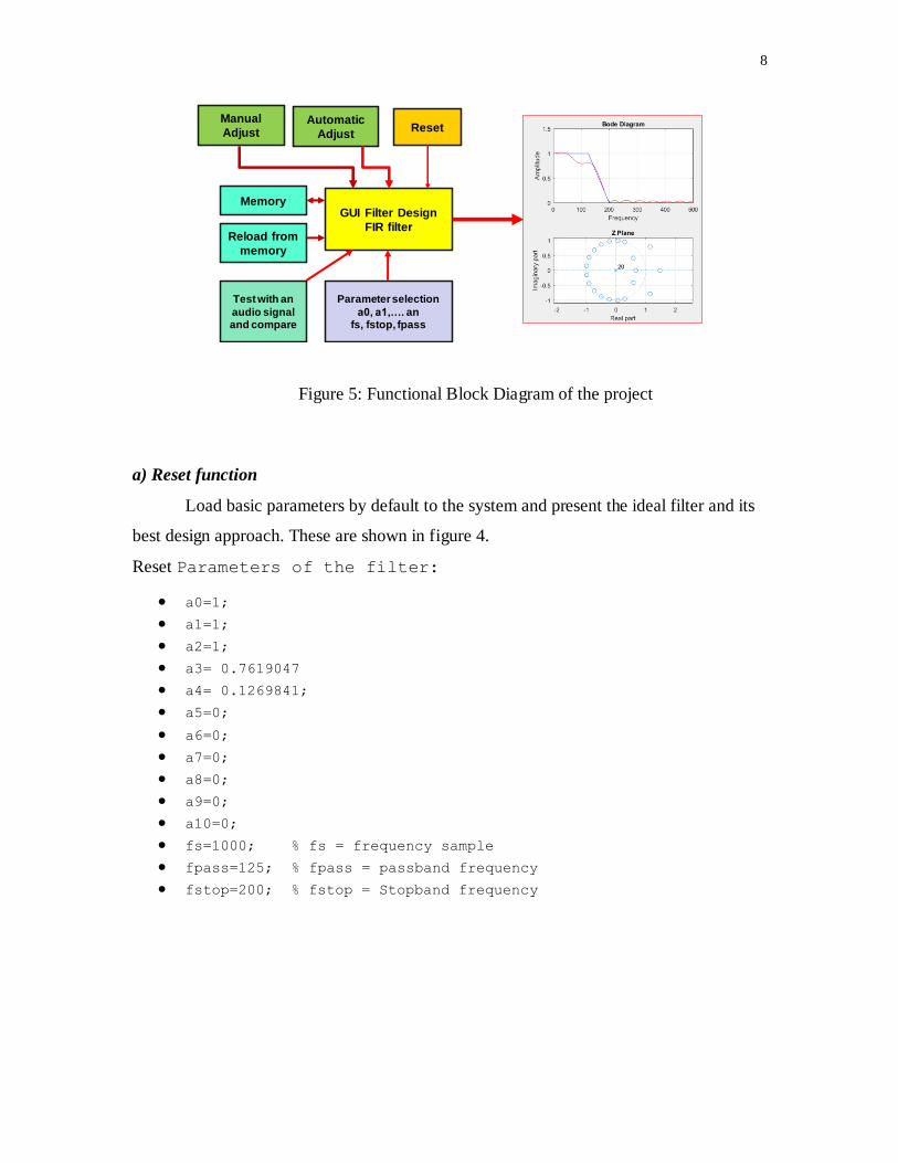
Figure 5: Functional Block Diagram of the project
a) Reset function
Load basic parameters by default to the system and present the ideal filter and its
best design approach. These are shown in figure 4.
Reset Parameters of the filter:
a0=1;
a1=1;
a2=1;
a3= 0.7619047
a4= 0.1269841;
a5=0;
a6=0;
a7=0;
a8=0;
a9=0;
a10=0;
fs=1000; % fs = frequency sample
fpass=125; % fpass = passband frequency
fstop=200; % fstop = Stopband frequency
9
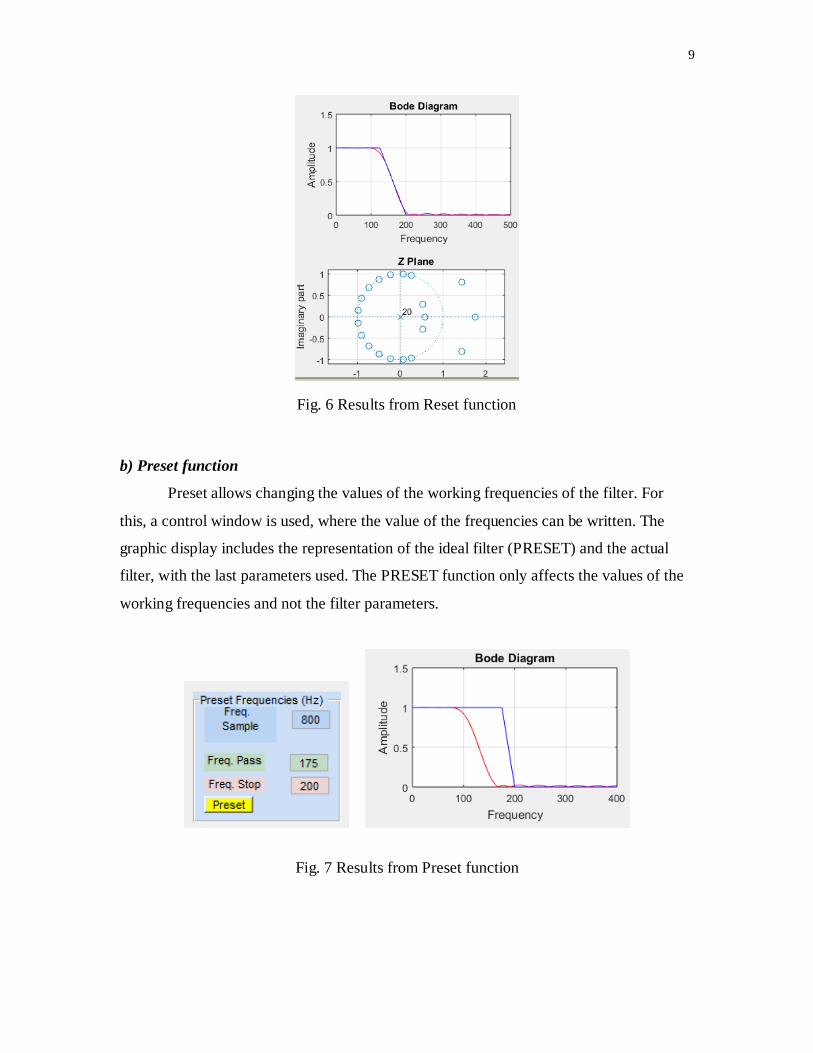
Fig. 6 Results from Reset function
b) Preset function
Preset allows changing the values of the working frequencies of the filter. For
this, a control window is used, where the value of the frequencies can be written. The
graphic display includes the representation of the ideal filter (PRESET) and the actual
filter, with the last parameters used. The PRESET function only affects the values of the
working frequencies and not the filter parameters.
Fig. 7 Results from Preset function
10
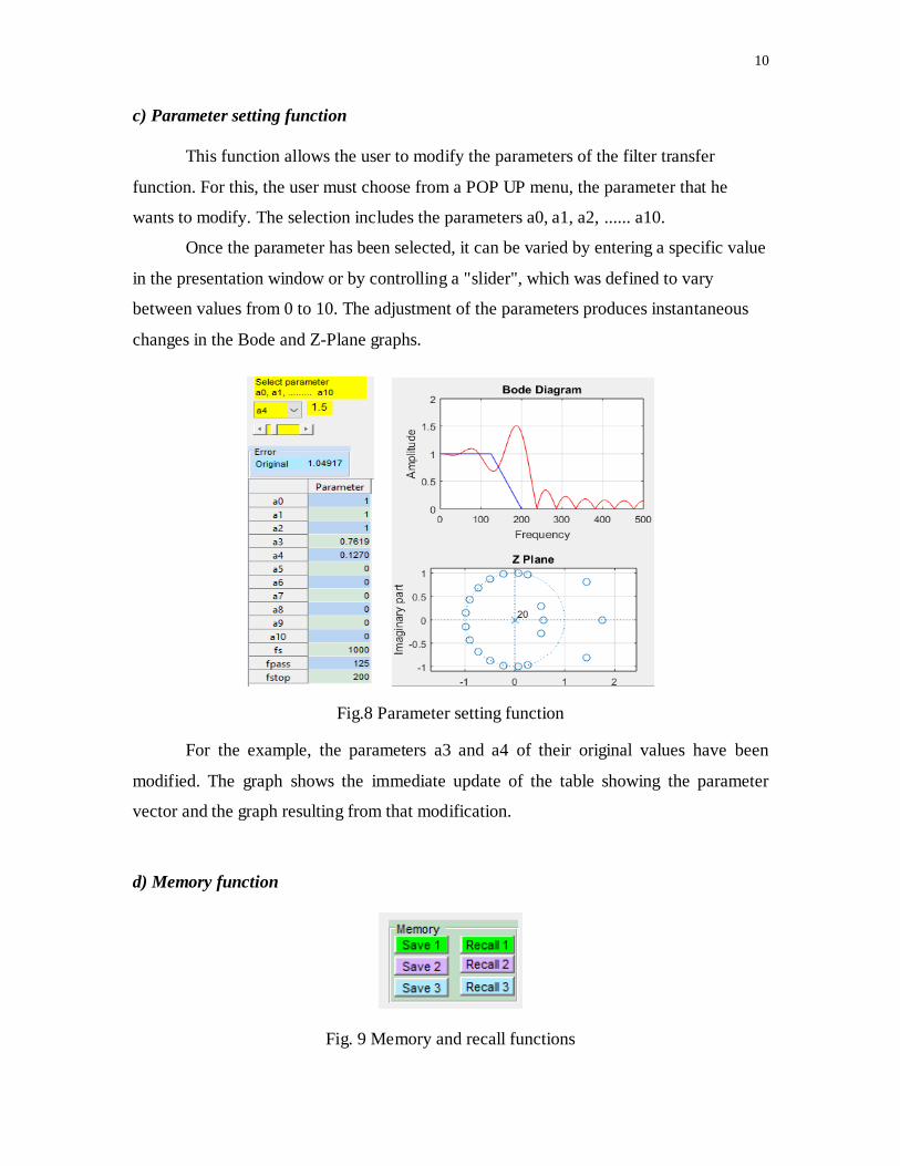
c) Parameter setting function
This function allows the user to modify the parameters of the filter transfer
function. For this, the user must choose from a POP UP menu, the parameter that he
wants to modify. The selection includes the parameters a0, a1, a2, ...... a10.
Once the parameter has been selected, it can be varied by entering a specific value
in the presentation window or by controlling a "slider", which was defined to vary
between values from 0 to 10. The adjustment of the parameters produces instantaneous
changes in the Bode and Z-Plane graphs.
Fig.8 Parameter setting function
For the example, the parameters a3 and a4 of their original values have been
modified. The graph shows the immediate update of the table showing the parameter
vector and the graph resulting from that modification.
d) Memory function
Fig. 9 Memory and recall functions
11
The memory function provides a working window where the user can record up to
three sets of data associated with the analysis of a filter. The work window has a couple
of buttons for each memory. The first has the function of recording and the second that of
loading the data stored in that memory position.
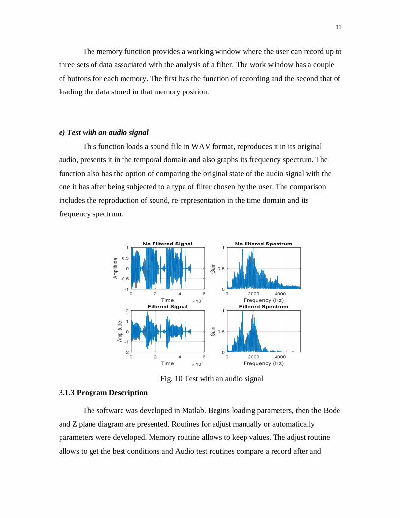
e) Test with an audio signal
This function loads a sound file in WAV format, reproduces it in its original
audio, presents it in the temporal domain and also graphs its frequency spectrum. The
function also has the option of comparing the original state of the audio signal with the
one it has after being subjected to a type of filter chosen by the user. The comparison
includes the reproduction of sound, re-representation in the time domain and its
frequency spectrum.
Fig. 10 Test with an audio signal
3.1.3 Program Description
The software was developed in Matlab. Begins loading parameters, then the Bode
and Z plane diagram are presented. Routines for adjust manually or automatically
parameters were developed. Memory routine allows to keep values. The adjust routine
allows to get the best conditions and Audio test routines compare a record after and
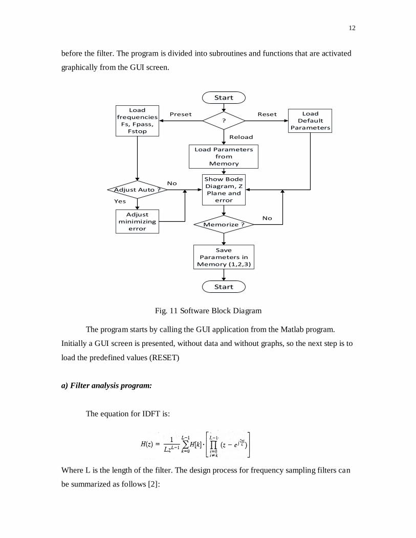
12
before the filter. The program is divided into subroutines and functions that are activated
graphically from the GUI screen.
Start
?Load
Default Parameters
Show Bode Diagram, Z Plane and
error
Load Parameters from
Memory
Reset
Reload
PresetLoad
frequencies Fs, Fpass,
Fstop
Adjust Auto ?No
Yes
Adjust minimizing
errorMemorize ?
No
Save Parameters in
Memory (1,2,3)
Start
Fig. 11 Software Block Diagram
The program starts by calling the GUI application from the Matlab program.
Initially a GUI screen is presented, without data and without graphs, so the next step is to
load the predefined values (RESET)
a) Filter analysis program:
The equation for IDFT is:
Where L is the length of the filter. The design process for frequency sampling filters can
be summarized as follows [2]:
13
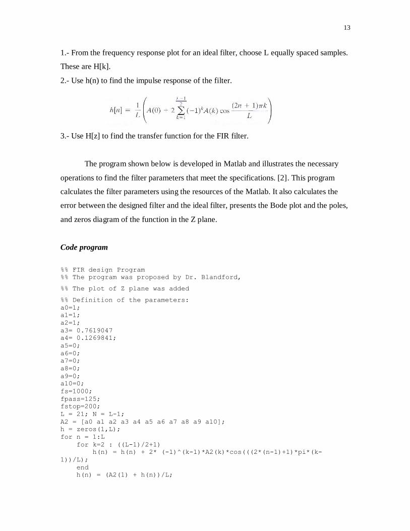
1.- From the frequency response plot for an ideal filter, choose L equally spaced samples.
These are H[k].
2.- Use h(n) to find the impulse response of the filter.
3.- Use H[z] to find the transfer function for the FIR filter.
The program shown below is developed in Matlab and illustrates the necessary
operations to find the filter parameters that meet the specifications. [2]. This program
calculates the filter parameters using the resources of the Matlab. It also calculates the
error between the designed filter and the ideal filter, presents the Bode plot and the poles,
and zeros diagram of the function in the Z plane.
Code program
%% FIR design Program
%% The program was proposed by Dr. Blandford,
%% The plot of Z plane was added
%% Definition of the parameters:
a0=1; a1=1; a2=1; a3= 0.7619047 a4= 0.1269841; a5=0; a6=0; a7=0; a8=0; a9=0; a10=0; fs=1000; fpass=125; fstop=200; L = 21; N = L-1; A2 = [a0 a1 a2 a3 a4 a5 a6 a7 a8 a9 a10]; h = zeros(1,L); for n = 1:L for k=2 : ((L-1)/2+1) h(n) = h(n) + 2* (-1)^(k-1)*A2(k)*cos(((2*(n-1)+1)*pi*(k-
1))/L); end h(n) = (A2(1) + h(n))/L;
14
end [H f] = freqz(h, 1, 4096, fs);
plot(f, abs(H), 'r'); xlabel('Frequency'); ylabel('Amplitude'); title ('Bode Diagram'); grid on;
m = -1/(fstop - fpass); b = -m*fstop; HId = m*f + b; % Ideal filter HId(HId > 1) = 1; HId(HId < 0) = 0; hold on; plot(f, HId, 'b');
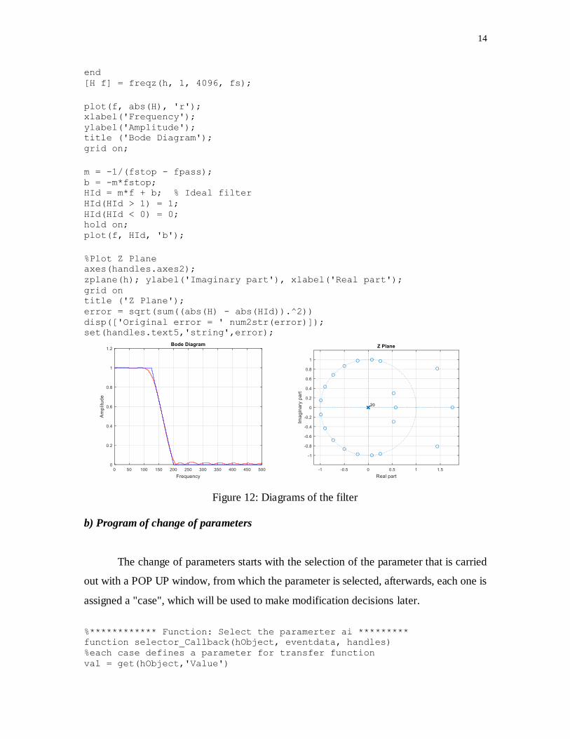
%Plot Z Plane axes(handles.axes2); zplane(h); ylabel('Imaginary part'), xlabel('Real part'); grid on title ('Z Plane'); error = sqrt(sum((abs(H) - abs(HId)).^2)) disp(['Original error = ' num2str(error)]); set(handles.text5,'string',error);
Figure 12: Diagrams of the filter
b) Program of change of parameters
The change of parameters starts with the selection of the parameter that is carried
out with a POP UP window, from which the parameter is selected, afterwards, each one is
assigned a "case", which will be used to make modification decisions later.
%************ Function: Select the paramerter ai ********* function selector_Callback(hObject, eventdata, handles) %each case defines a parameter for transfer function val = get(hObject,'Value')
15
switch val case 1 S.temp = 1 case 2 S.temp = 2 case 3 S.temp = 3 case 4 S.temp = 4 case 5 S.temp = 5 case 6 S.temp = 6 case 7 S.temp = 7 case 8 S.temp = 8 case 9 S.temp = 9 case 10 S.temp = 10 case 11 S.temp = 11 otherwise end set(handles.selector, 'UserData', S); % end of parameter slection from Pop Up menu ***********
After selecting the parameter, we proceed to vary its value with the use of the "slider":
%******************* Function: Slider ***************** %Assign slider value to a ai %temp is a output parameter from pop up table (VARIES FROM 0 TO 11) temp = get(handles.selector, 'Value'); % Selecting ai if temp == 1 a0=ax elseif temp == 2 a1=ax elseif temp == 3 a2=ax elseif temp == 4 a3=ax elseif temp == 5 a4=ax elseif temp == 6 a5=ax elseif temp == 7 a6=ax elseif temp == 8 a7=ax elseif temp == 9 a8=ax elseif temp == 10 a9=ax elseif temp == 11
16
a10=ax else a10=ax end set(handles.text2,'string',ax);
c) Memory and loading program
The memory function uses a vector in which it stores the data and loads it again
when needed. The vector includes, in addition to the parameters, the frequency values
used. The parameters to be saved are taken from the dynamic table of instantaneous
presentation of the data:
A33=get(handles.uitable2,'Data'); A44_mem1=A33([1 2 3 4 5 6 7 8 9 10 11 12 13 14]) fs_mem1=A33([12]) fpass_mem1=A33([13]); fstop_mem1=A33([14]);
The loading of the data in memory:
A_mem1=A44_mem1([1 2 3 4 5 6 7 8 9 10 11]) fs=A44_mem1([12]) fpass=A44_mem1([13]) fstop=A44_mem1([14])
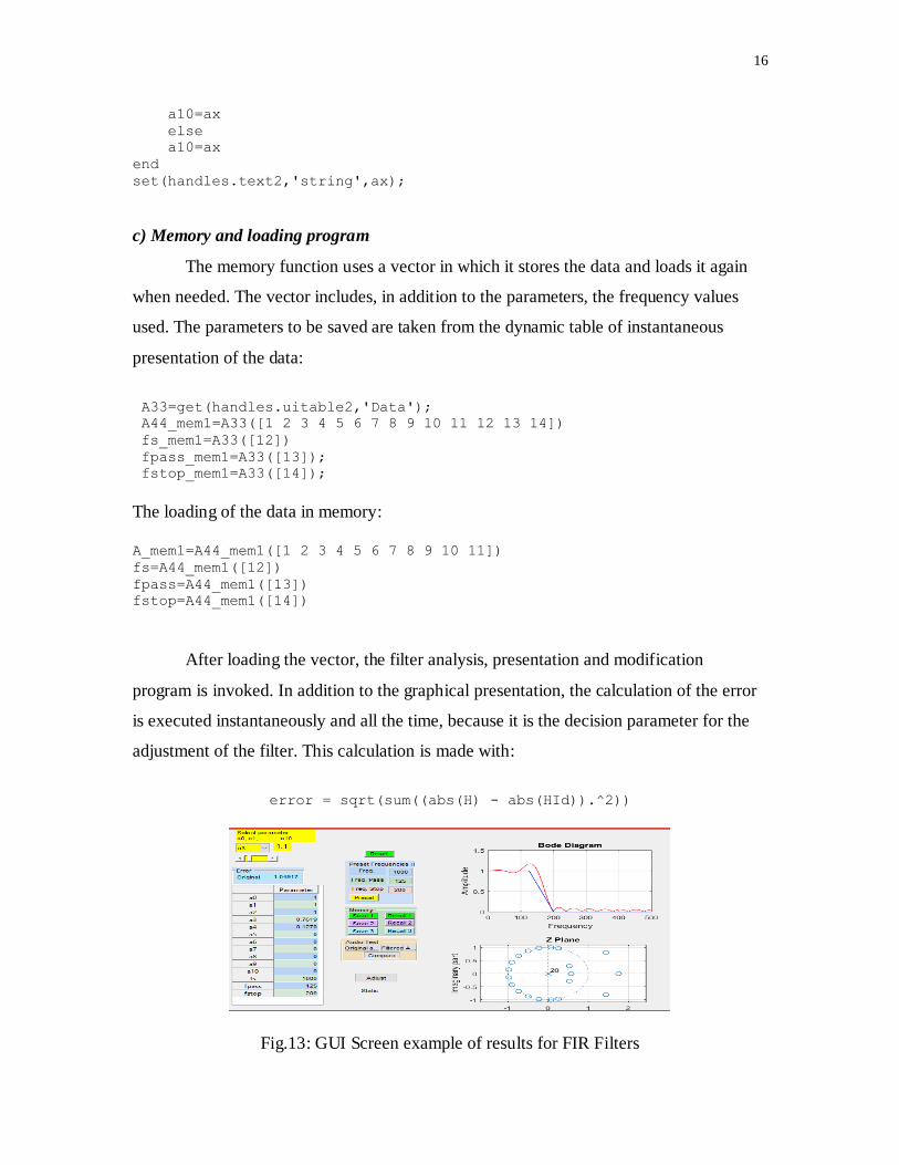
After loading the vector, the filter analysis, presentation and modification
program is invoked. In addition to the graphical presentation, the calculation of the error
is executed instantaneously and all the time, because it is the decision parameter for the
adjustment of the filter. This calculation is made with:
error = sqrt(sum((abs(H) - abs(HId)).^2))
Fig.13: GUI Screen example of results for FIR Filters
17
3.2 IIR FILTERS
IIR filters have feedback, which results in a transfer function that has poles at
locations other than the origin [2]. The poles, depending on how close they are to the unit
circle, cause the gain to increase at a particular frequency. In the design of IIR filters, we
need to figure out where to place the zeros to decrease the gain and where to place the
poles to make it increase. This is the reason for which the interaction with poles and zeros
in Z plane was choose as a technique for analysis of IIR filters. Using IIR, the design
results with narrower transition bands than comparable FIR filters.
Because IIR filters have a feedback, it is possible that they can be unstable,
whereas with FIR, the stability is a given. The feed back causes other problems indirectly
tied to stability that has to do with noise. FIR filters are always linear phase. For a IIR
filter linear phase across the 0 to fs/2 frequency band is impossible.
3.2.1 GUI DESIGN
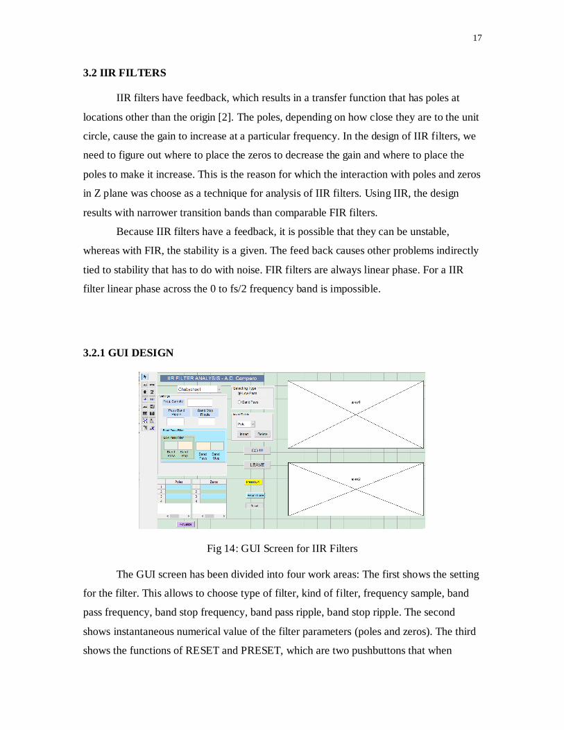
Fig 14: GUI Screen for IIR Filters
The GUI screen has been divided into four work areas: The first shows the setting
for the filter. This allows to choose type of filter, kind of filter, frequency sample, band
pass frequency, band stop frequency, band pass ripple, band stop ripple. The second
shows instantaneous numerical value of the filter parameters (poles and zeros). The third
shows the functions of RESET and PRESET, which are two pushbuttons that when
18
activated load the data by default (RESET) or the selected values (PRESET), and the
insert/delete poles and zeros commands that allow to add or erase poles or. The fourth is
the graphic work area, where the diagrams of Bode and Z plane (axes 1 and axes 2) are
presented.
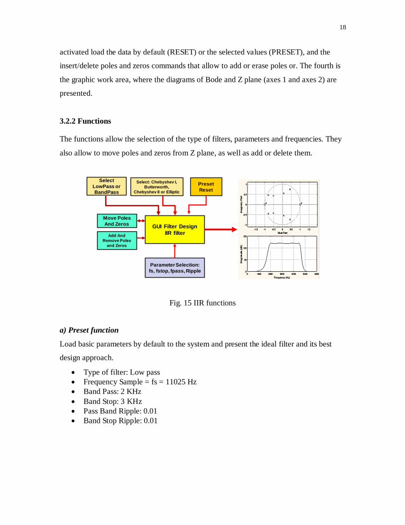
3.2.2 Functions
The functions allow the selection of the type of filters, parameters and frequencies. They
also allow to move poles and zeros from Z plane, as well as add or delete them.
GUI Filter Design
IIR filter
Parameter Selection:
fs, fstop, fpass, Ripple
Move Poles
And Zeros
Add And
Remove Poles
and Zeros
Select: Chebyshev I,
Butterworth,
Chebyshev II or Elliptic
Preset
Reset
Select
LowPass orBandPass
Fig. 15 IIR functions
a) Preset function
Load basic parameters by default to the system and present the ideal filter and its best
design approach.
Type of filter: Low pass
Frequency Sample = fs = 11025 Hz
Band Pass: 2 KHz
Band Stop: 3 KHz
Pass Band Ripple: 0.01
Band Stop Ripple: 0.01
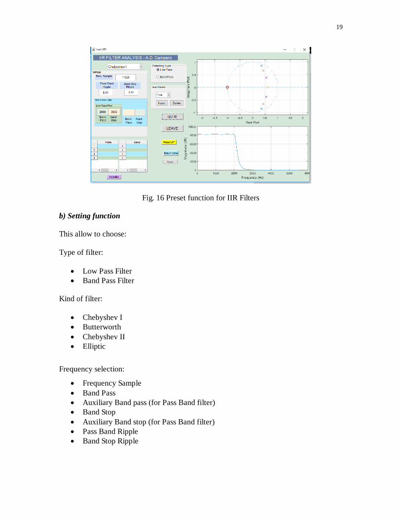
19
Fig. 16 Preset function for IIR Filters
b) Setting function
This allow to choose:
Type of filter:
Low Pass Filter
Band Pass Filter
Kind of filter:
Chebyshev I
Butterworth
Chebyshev II
Elliptic
Frequency selection:
Frequency Sample
Band Pass
Auxiliary Band pass (for Pass Band filter)
Band Stop
Auxiliary Band stop (for Pass Band filter)
Pass Band Ripple
Band Stop Ripple
20
c) Visualizing Poles and zeros function
There is a table in which poles and zeros are presented (numerical values). The table has
a push button in order to actualize values when and adjust is made.
d) Execute or leave function
Pushbuttons were implemented in order to execute the program taking in account the
parameters, leave the program or return to the home page. The execution uses Matlab
resources for the filters.
e) Modify Pole and zeros function
This function allows to modify poles and zeros from the graph in a flexible and dynamic
way. The functions allow to use the mouse/cursor in order to catch a pole or zero and
move it along the z plane. Whenever a pole or zero is moving its conjugates moves as
well. The movement of poles or zeros in the z plane immediately produce a modification
of the Bode diagram.
f) Insert Poles or Zeros Function
This function allows to insert poles or zeros in the z plane. Whenever a pole is inserted, a
single pole appears in the right plane on the axis. If the pole is moved in the z plane it
will generate its conjugate in an automatic mode. Whenever a Zero is added, it will
appear in the left-hand axis and as the poles, it can be moves along the z plane generating
its conjugate.
g) Reset Function
This function has a pushbutton in order to clear all values and graphics.
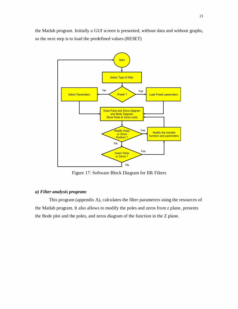
3.2.3 Program Description
The program is divided into subroutines and functions that are activated
graphically from the GUI screen. The program starts by calling the GUI application from
21
the Matlab program. Initially a GUI screen is presented, without data and without graphs,
so the next step is to load the predefined values (RESET)
Select Type of filter
Load Preset parameters
Start
Preset ?
Yes
No
Yes
Draw Poles and Zeros diagramand Bode Diagram
Show Poles & Zeros roots
Select Parameters
No
Modify Polesor ZerosPosition ?
Modify the transfer function and parameters
Insert Polesor Zeros ?
Yes
No
Figure 17: Software Block Diagram for IIR Filters
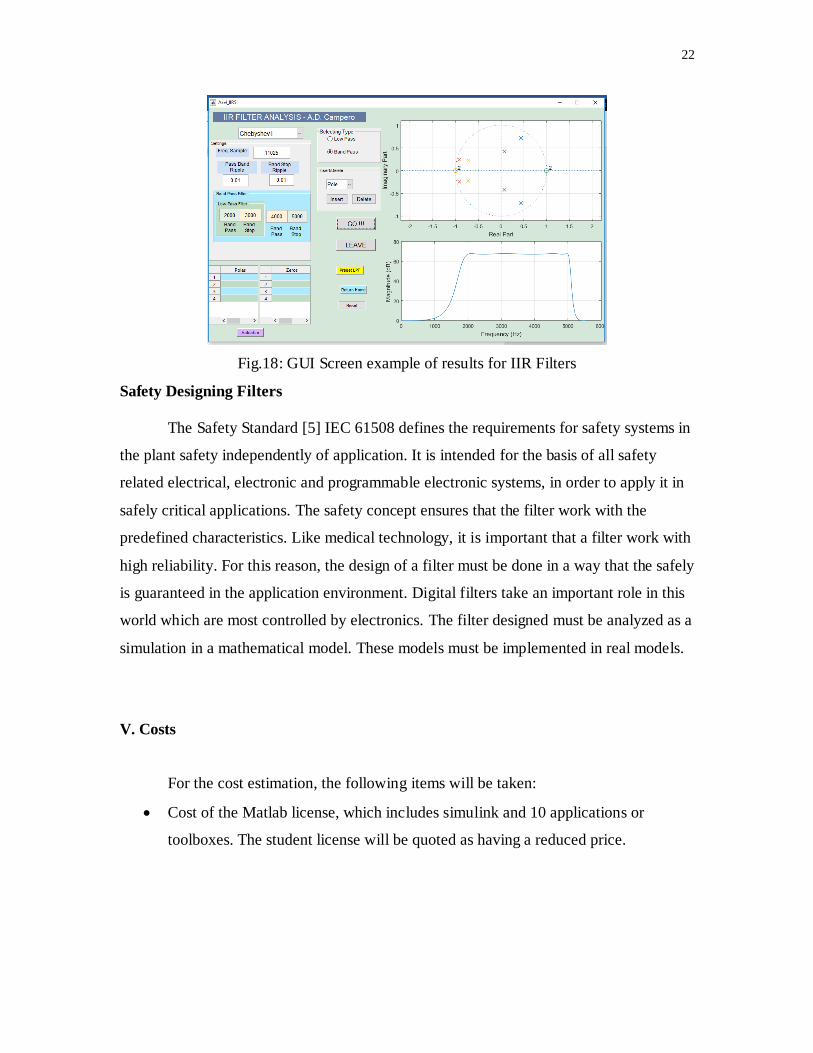
a) Filter analysis program:
This program (appendix A), calculates the filter parameters using the resources of
the Matlab program. It also allows to modify the poles and zeros from z plane, presents
the Bode plot and the poles, and zeros diagram of the function in the Z plane.
22
Fig.18: GUI Screen example of results for IIR Filters
Safety Designing Filters
The Safety Standard [5] IEC 61508 defines the requirements for safety systems in
the plant safety independently of application. It is intended for the basis of all safety
related electrical, electronic and programmable electronic systems, in order to apply it in
safely critical applications. The safety concept ensures that the filter work with the
predefined characteristics. Like medical technology, it is important that a filter work with
high reliability. For this reason, the design of a filter must be done in a way that the safely
is guaranteed in the application environment. Digital filters take an important role in this
world which are most controlled by electronics. The filter designed must be analyzed as a
simulation in a mathematical model. These models must be implemented in real models.
V. Costs
For the cost estimation, the following items will be taken:
Cost of the Matlab license, which includes simulink and 10 applications or
toolboxes. The student license will be quoted as having a reduced price.
23
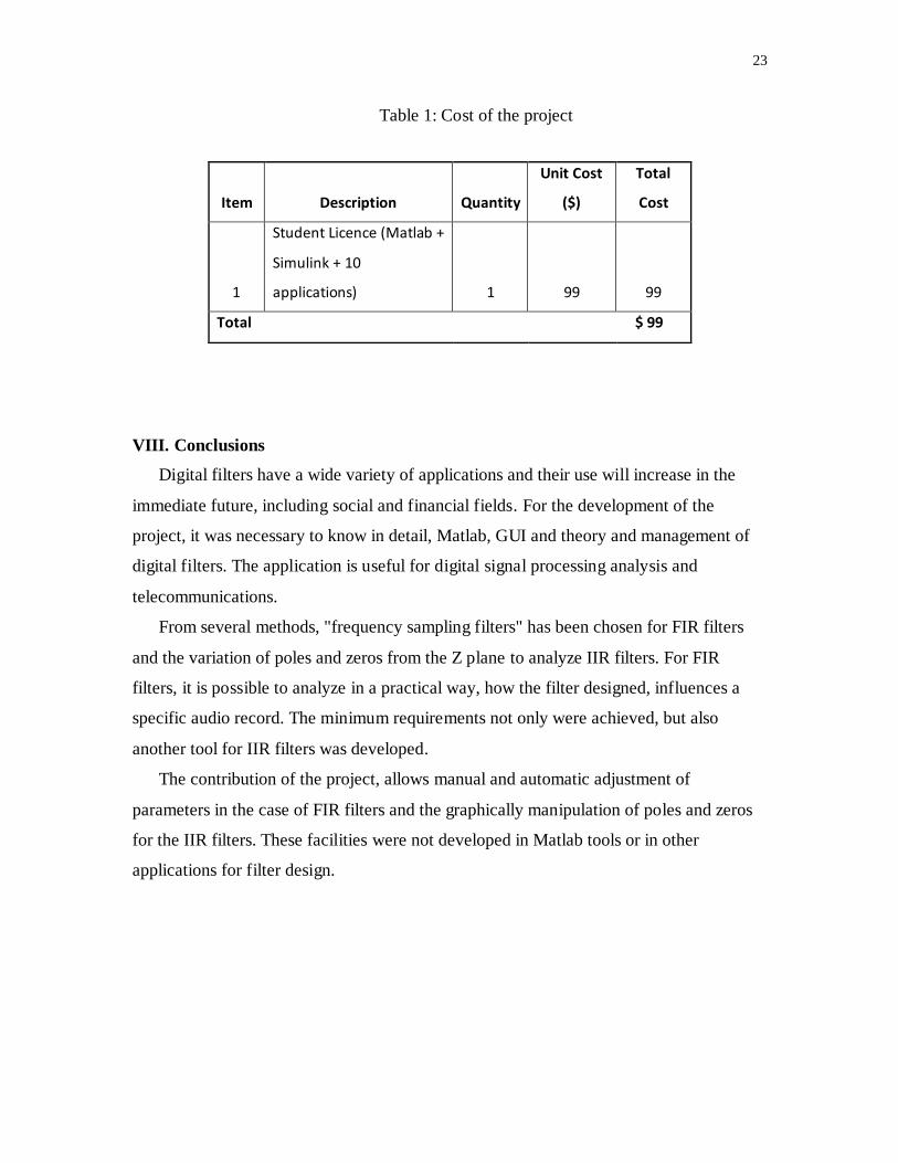
Table 1: Cost of the project
Item Description Quantity
Unit Cost
($)
Total
Cost
1
Student Licence (Matlab +
Simulink + 10
applications) 1 99 99
Total $ 99
VIII. Conclusions
Digital filters have a wide variety of applications and their use will increase in the
immediate future, including social and financial fields. For the development of the
project, it was necessary to know in detail, Matlab, GUI and theory and management of
digital filters. The application is useful for digital signal processing analysis and
telecommunications.
From several methods, "frequency sampling filters" has been chosen for FIR filters
and the variation of poles and zeros from the Z plane to analyze IIR filters. For FIR
filters, it is possible to analyze in a practical way, how the filter designed, influences a
specific audio record. The minimum requirements not only were achieved, but also
another tool for IIR filters was developed.
The contribution of the project, allows manual and automatic adjustment of
parameters in the case of FIR filters and the graphically manipulation of poles and zeros
for the IIR filters. These facilities were not developed in Matlab tools or in other
applications for filter design.
24
Appendix A: Code for FIR Filters Analysis
%Axel Daniela Campero Vega
%IIR Filter design and analysis %University of Evansville
function varargout = Axel_IIR5(varargin)
clc;
gui_Singleton = 1; gui_State = struct('gui_Name', mfilename, ...
'gui_Singleton', gui_Singleton, ... 'gui_OpeningFcn', @Axel_IIR5_OpeningFcn, ...
'gui_OutputFcn', @Axel_IIR5_OutputFcn, ...
'gui_LayoutFcn', [] , ... 'gui_Callback', []);
if nargin && ischar(varargin{1}) gui_State.gui_Callback = str2func(varargin{1});
end
if nargout
[varargout{1:nargout}] = gui_mainfcn(gui_State, varargin{:}); else
gui_mainfcn(gui_State, varargin{:});
end
function Axel_IIR5_OpeningFcn(hObject, eventdata, handles, varargin) handles.output = hObject;
guidata(hObject, handles);
function varargout = Axel_IIR5_OutputFcn(hObject, eventdata, handles)
varargout{1} = handles.output;
%*********************************************************
function sel1_Callback(hObject, eventdata, handles) global contador
fun = get(handles.sel1,'Value'); switch fun
case 1
contador=1 case 2
contador=2 case 3
contador=3; case 4
contador=4;
25
end
guidata(hObject, handles); function sel1_CreateFcn(hObject, eventdata, handles)
if ispc && isequal(get(hObject,'BackgroundColor'), get(0,'defaultUicontrolBackgroundColor'))
set(hObject,'BackgroundColor','white');
end %************************************************
function edit3_Callback(hObject, eventdata, handles) Val=get(hObject,'string');
NewVal=str2double(Val);
handles.edit3=NewVal; guidata(hObject,handles);
function edit3_CreateFcn(hObject, eventdata, handles) if ispc && isequal(get(hObject,'BackgroundColor'),
get(0,'defaultUicontrolBackgroundColor'))
set(hObject,'BackgroundColor','white'); end
%***************************************************** function edit4_Callback(hObject, eventdata, handles)
Val=get(hObject,'string');
NewVal=str2double(Val); handles.edit4=NewVal;
guidata(hObject,handles);
function edit4_CreateFcn(hObject, eventdata, handles)
if ispc && isequal(get(hObject,'BackgroundColor'), get(0,'defaultUicontrolBackgroundColor'))
set(hObject,'BackgroundColor','white'); end
%***************************************************
function edit5_Callback(hObject, eventdata, handles) Val=get(hObject,'string');
NewVal=str2double(Val); handles.edit5=NewVal;
guidata(hObject,handles);
function edit5_CreateFcn(hObject, eventdata, handles)
if ispc && isequal(get(hObject,'BackgroundColor'), get(0,'defaultUicontrolBackgroundColor'))
set(hObject,'BackgroundColor','white');
end %******************************************************
function edit6_Callback(hObject, eventdata, handles) Val=get(hObject,'string');
NewVal=str2double(Val);
26
handles.edit6=NewVal;
guidata(hObject,handles);
function edit6_CreateFcn(hObject, eventdata, handles) if ispc && isequal(get(hObject,'BackgroundColor'),
get(0,'defaultUicontrolBackgroundColor'))
set(hObject,'BackgroundColor','white'); end
%******************************************************* function edit7_Callback(hObject, eventdata, handles)
Val=get(hObject,'string');
NewVal=str2double(Val); handles.edit7=NewVal;
guidata(hObject,handles);
function edit7_CreateFcn(hObject, eventdata, handles)
if ispc && isequal(get(hObject,'BackgroundColor'), get(0,'defaultUicontrolBackgroundColor'))
set(hObject,'BackgroundColor','white'); end
%************************************************
function edit8_Callback(hObject, eventdata, handles) Val=get(hObject,'string');
NewVal=str2double(Val); handles.edit8=NewVal;
guidata(hObject,handles);
function edit8_CreateFcn(hObject, eventdata, handles)
if ispc && isequal(get(hObject,'BackgroundColor'), get(0,'defaultUicontrolBackgroundColor'))
set(hObject,'BackgroundColor','white');
end %**********************************************************
function edit9_Callback(hObject, eventdata, handles) Val=get(hObject,'string');
NewVal=str2double(Val);
handles.edit9=NewVal; guidata(hObject,handles);
function edit9_CreateFcn(hObject, eventdata, handles)
if ispc && isequal(get(hObject,'BackgroundColor'),
get(0,'defaultUicontrolBackgroundColor')) set(hObject,'BackgroundColor','white');
end %***********************************************************
function pushbutton1_Callback(hObject, eventdata, handles)
27
global zh ph b a z rety p pt zr
global ax1 ax2 global contador2 contador
fs=handles.edit3 fps1=handles.edit6
fst1=handles.edit7
Rp=handles.edit4 Rs=handles.edit5
fps2=handles.edit9 fst2=handles.edit8
[m1,n1]=size(contador2)
[m2,n2]=size(contador) %Seleccion de tipos de filtros
if (m1==0 & n1==0) contador2=1;
end
if contador2==1 RsDB=-20*log10(Rs);
RpDB=-20*log10(1-Rp); Wp=fps1/(fs/2)
Ws=fst1/(fs/2)
elseif contador2==2 fps=[fps1 fps2]
fst=[fst1 fst2] RsDB=-20*log10(Rs)
RpDB=-20*log10(1-Rp)
Wp=fps/(fs/2) Ws=fst/(fs/2)
end
if (m2==0 & n2==0)
contador=1; end
if contador==1 [Nc,Wnc] = cheb1ord(Wp,Ws,RpDB,RsDB);
[num den]=cheby1(Nc,RpDB,Wnc)
elseif contador==2 [Nc,Wnc] = buttord(Wp,Ws,RpDB,RsDB);
[num den]=butter(Nc,Wnc); elseif contador==3
[Nc,Wnc] = cheb2ord(Wp,Ws,RpDB,RsDB);
[num den]=cheby2(Nc,RpDB,Wnc); elseif contador==4
[Nc,Wnc] = ellipord(Wp,Ws,RpDB,RsDB); [num den]=ellip(Nc,RpDB,RsDB,Wnc);
end
28
[z,p,k] = tf2zp(num,den); p=p';
z=z'; A=[num den];
axes(handles.axes1);
bl=roots(num); %los zeros al=roots(den); %los polos
ax=[]; %creamos un vector de N dimensiones para los zeros bx=[]; %creamos un vector de N dimensiones para los polos
k=1;
i=1; var1=length(bl);
while (k~=var1)
if (bl(k)==conj(bl(k+1)))
ax(1,i)=bl(k); ax(2,i)=bl(k+1);
k=k+2; %Incremento para el salto de dos i=i+1;
if (k>var1)
break; end
else ax(1,i)=bl(k);
ax(2,i)=NaN;
k=k+1; %Incremento para el salto de uno i=i+1;
if (k>var1) break;
end
end end
k=1; i=1;
var2=length(al);
while (k~=var2) if (al(k)==conj(al(k+1)))
bx(1,i)=al(k); bx(2,i)=al(k+1);
k=k+2; %Incremento para el salto de dos
i=i+1; if (k>var2)
break; end
else
29
bx(1,i)=al(k);
bx(2,i)=NaN; k=k+1; %Incremento para el salto de uno
i=i+1; if (k>var2)
break;
end end
end
[zh,ph]=zplaneplot(ax,bx);
grid on ax1 = gca;
ylabel('Imaginary Part') xlabel('Real Part')
rety = handles.axes2; axes(rety);
p=p'; z=z';
[b,a]=zp2tf(z,p,k);
[H f]=freqz(b,a,1024,fs); global Hz;
global az; global bz;
Hz=H;
az=a; bz=b;
plot(f,abs(H));
grid on
ax2 = gca; xlabel('Frequency (Hz)')
ylabel('Magnitude (dB) ')
set(zh,'buttondownfcn','FILTROS(''zeroclick'')',...
'markersize',8,'linewidth',1) set(ph,'buttondownfcn','FILTROS(''poleclick'')',...
'markersize',8,'linewidth',1)
function pushbutton2_Callback(hObject, eventdata, handles)
global zh ph b a z rety p pt zr global ax1 ax2
global contador3 contador4 [m11,n11]=size(contador3)
[m22,n22]=size(contador4)
30
if (m11==0 & n11==0 & m22==0 & n22==0)
contador3=1; contador4=1;
end size(contador4)
if (contador3==1 & contador4==1) %Opcion POLO SIMPLE
if length(ph)>0 ph(end+1) = line([0.5 NaN],[0 0], 'parent', ax1, 'buttondownfcn',
'FILTROS(''poleclick'')',... 'markersize',8,'linewidth',1,'marker','x','linestyle','none');
else
ph = line(.5,0,'parent',ax1,'buttondownfcn','FILTROS(''poleclick'')',... 'markersize',8,'linewidth',1,'marker','x','linestyle','none');
set(findobj('string','BORRAR POLO'),'enable','on') end
FILTROS('recompute')
elseif (contador3==1 & contador4==2) %Opcion POLO CONJUGADO
if length(ph)>0 ph(end+1) = line([0.5 0.5],[0.5 -0.5], 'parent', ax1, 'buttondownfcn',
'FILTROS(''poleclick'')',...
'markersize',8,'linewidth',1,'marker','x','linestyle','none'); else
ph = line(.5,0,'parent',ax1,'buttondownfcn','FILTROS(''poleclick'')',... 'markersize',8,'linewidth',1,'marker','x','linestyle','none');
set(findobj('string','BORRAR POLO'),'enable','on')
end FILTROS('recompute')
elseif (contador3==2 & contador4==1) %Opcion ZERO SIMPLE
if length(zh)>0
zh(end+1) = line([-0.5 NaN],[0 0], 'parent' ,ax1, 'buttondownfcn', 'FILTROS(''zeroclick'')',...
'markersize',8,'linewidth',1,'marker','o','linestyle','none'); else
zh = line(.5,0,'parent',ax1,'buttondownfcn','FILTROS(''zeroclick'')',...
'markersize',8,'linewidth',1,'marker','o','linestyle','none'); set(findobj('string','BORRAR CERO'),'enable','on')
end FILTROS('recompute')
elseif (contador3==2 & contador4==2) %Opcion ZERO CONJUGADO
if length(zh)>0 zh(end+1) = line([-0.5 -0.5],[-0.5 0.5],
'parent',ax1,'buttondownfcn','FILTROS(''zeroclick'')',... 'markersize',8,'linewidth',1,'marker','o','linestyle','none');
else
31
zh = line(.5,0,'parent',ax1,'buttondownfcn','FILTROS(''zeroclick'')',...
'markersize',8,'linewidth',1,'marker','o','linestyle','none'); set(findobj('string','BORRAR CERO'),'enable','on')
end FILTROS('recompute')
end
%********************************************* function pushbutton3_Callback(hObject, eventdata, handles)
global zh ph b a z rety p pt zr global ax1 ax2
global contador3
if contador3==1 %Opcion para eliminar POLOS
delete(ph(end)) ph(end)=[];
if length(ph)==0
set(gco,'enable','off') end
FILTROS('recompute') elseif contador3==2 %Opcion para eliminar ZEROS
delete(zh(end))
zh(end)=[]; if length(zh)==0
set(gco,'enable','off') end
FILTROS('recompute')
end
function uipanel1_SelectionChangeFcn(hObject, eventdata, handles) global contador2
if (hObject==handles.uno)
contador2=1 elseif (hObject==handles.dos)
contador2=2 else
contador2=1
end
function sel2_Callback(hObject, eventdata, handles) global contador3
fun = get(handles.sel2,'Value');
switch fun case 1
contador3=1 case 2
contador3=2
32
end
guidata(hObject, handles);
function sel2_CreateFcn(hObject, eventdata, handles) if ispc && isequal(get(hObject,'BackgroundColor'),
get(0,'defaultUicontrolBackgroundColor'))
set(hObject,'BackgroundColor','white'); end
function uipanel2_SelectionChangeFcn(hObject, eventdata, handles)
global contador4
if (hObject==handles.tres) contador4=1
elseif (hObject==handles.cuatro) contador4=2
end
function pushbutton6_Callback(hObject, eventdata, handles)
global contador contador2 opc=questdlg('Do you want to leave the program?','LEAVE','YES','NO','NO');
if strcmp(opc,'NO')
return; end
contador=1; contador2=1;
delete(hObject);
clear,clc,close all
function pushbutton7_Callback(hObject, eventdata, handles) global datax dataxt
global datbx datbxt
set(handles.uitable1,'data',dataxt);
set(handles.uitable2,'data',datbxt); function uitable1_CellEditCallback(hObject, eventdata, handles)
function edit10_Callback(hObject, eventdata, handles)
clc
global fs fps1 fst1 Rp Rs; fs=11025;
fps1=2000;
fst1=3000; Rp=0.01;
Rs=0.01;
set(handles.edit3,'string',fs);
33
set(handles.edit4,'string',Rp);
set(handles.edit5,'string',Rs); set(handles.edit6,'string',fps1);
set(handles.edit7,'string',fst1);
handles.edit3 =fs;
handles.edit4 =Rp; handles.edit5 =Rs;
handles.edit6 =fps1; handles.edit7 =fst1;
guidata(hObject, handles)
function edit10_CreateFcn(hObject, eventdata, handles)
if ispc && isequal(get(hObject,'BackgroundColor'), get(0,'defaultUicontrolBackgroundColor'))
set(hObject,'BackgroundColor','white');
end
% --- Executes on button press in pushbutton8. function pushbutton8_Callback(hObject, eventdata, handles)
gui1;
% --- Executes on button press in pushbutton9.
function pushbutton9_Callback(hObject, eventdata, handles) clc
global fs fps1 fst1 Rp Rs; fs=11025;
fps1=2000; fst1=3000;
Rp=0.01;
Rs=0.01;
set(handles.edit3,'string',fs); set(handles.edit4,'string',Rp);
set(handles.edit5,'string',Rs);
set(handles.edit6,'string',fps1); set(handles.edit7,'string',fst1);
guidata(hObject, handles)
handles.edit3 =fs;
handles.edit4 =Rp; handles.edit5 =Rs;
handles.edit6 =fps1; handles.edit7 =fst1;
guidata(hObject, handles)

34
% --- Executes on button press in pushbutton10.
function pushbutton10_Callback(hObject, eventdata, handles) close Axel_IIR5
open Axel_IIR5 clearvars
run Axel_IIR5
% end of the program
35
References
[1] Matlab - Matworks Documentation: Digital Filters [Online]. Available:
https://www.mathworks.com/help/signal/ug/iir-filter-design.html
[2] Dick Blandford, Jhon Parr, “Introduction to Digital Signal Processing”. PEARSON,
2013
[3] Alexander D. Poularikas, “Signals and Systems Primer with MATLAB”, CRC Press,
2006 - Technology & Engineering
[4] Julius Orion Smith, “Spectral Audio Signal Processing”, Contributors Stanford University. Center for Computer Research in Music and Acoustics, Stanford University,
Publisher W3K, 2011
[5] Tomasz Nowakowski, Marek Młyńczak,, “Safety and Reliability: Methodology and
Applications”, CRC Press, Sep 18, 2014 - Technology & Engineering


![JUnit-Testing GUI Components [Autosaved]shsaad/seng426/resources/Lab Slides... · 2011-06-15 · JUnit-Testing GUI Components . Agenda Test GUI Components Simple GUI Application Test](https://img.pdfslide.us/doc/110x75/5e237780175e3d268e70f660/junit-testing-gui-components-autosaved-shsaadseng426resourceslab-slides.jpg)