Embed Size (px)
Citation preview

Guang Yang
Dynamic analyses ofa masonry buildingtested in a shaking TableDy
nam
ic a
naly
ses
of a
mas
onry
bui
ldin
g te
sted
in a
sha
king
tabl
eGu
ang
Yang
2010
Guang Yang
Dynamic analyses ofa masonry buildingtested in a shaking table
2010

Dynamic analyses of a masonry building tested in a shaking table
Erasmus Mundus Programme
ADVANCED MASTERS IN STRUCTURAL ANALYSIS OF MONUMENTS AND HISTORICAL CONSTRUCTIONS i
DECLARATION
Name: Guang Yang
Email: [email protected]
Title of the
Msc Dissertation: Dynamic analyses of a masonry building tested in a shaking table
Supervisor: Professor Doctor Paulo José Brandão Barbosa Lourenço
Year: 2010
I hereby declare that all information in this document has been obtained and presented in accordance with
academic rules and ethical conduct. I also declare that, as required by these rules and conduct, I have fully cited
and referenced all material and results that are not original to this work.
I hereby declare that the MSc Consortium responsible for the Advanced Masters in Structural Analysis of
Monuments and Historical Constructions is allowed to store and make available electronically the present MSc
Dissertation.
University: University of Minho
Date: July, 14th, 2010
Signature: ___________________________

Dynamic analyses of a masonry building tested in a shaking table
Erasmus Mundus Programme
ii ADVANCED MASTERS IN STRUCTURAL ANALYSIS OF MONUMENTS AND HISTORICAL CONSTRUCTIONS

Dynamic analyses of a masonry building tested in a shaking table
Erasmus Mundus Programme
ADVANCED MASTERS IN STRUCTURAL ANALYSIS OF MONUMENTS AND HISTORICAL CONSTRUCTIONS iii
献给我的母亲和天堂中的父亲
献给我挚爱的未婚妻周爽

Dynamic analyses of a masonry building tested in a shaking table
Erasmus Mundus Programme
iv ADVANCED MASTERS IN STRUCTURAL ANALYSIS OF MONUMENTS AND HISTORICAL CONSTRUCTIONS
Dynamic analyses of a masonry building tested in a shaking table
Erasmus Mundus Programme
ADVANCED MASTERS IN STRUCTURAL ANALYSIS OF MONUMENTS AND HISTORICAL CONSTRUCTIONS v
AAcckknnoowwlleeddggeemmeennttss
This dissertation would not be completed without the help of all that, directly or indirectly,
were involved in my work and successfully contributed to its conclusion. Among the different
support, I would like to express my gratitude to:
• Professor Paulo Lourenço, my supervisor and mentor, for his full support and
encouragement, the interesting discussions, patience and careful reading;
• PhD student Nuno Mendes, my colleague and friend, for his tremendous help and
support in the modeling and many ideas of the dissertation;
• the Erasmus Mundus Committee and European Union, for fully support me with
the scholarship to finish the master study;
• Mr. David Biggs, P.E from U.S, for his advice in the English writing;
Finally, I would like to make a special acknowledgment to my family:
• Lihong Gao, my mother, for her kindness and encourage during this four month,
and most importantly, the courage to move on after my father left;
• Zhaoxi Yang, my father in heaven, for all he did to make my dream of studying
abroad come true, and the good memories he left for me, rest in peace;
• Shuang Zhou, my fiancée and love of my entire life, for her patience and endless
love during this year.

Dynamic analyses of a masonry building tested in a shaking table
Erasmus Mundus Programme
vi ADVANCED MASTERS IN STRUCTURAL ANALYSIS OF MONUMENTS AND HISTORICAL CONSTRUCTIONS
Dynamic analyses of a masonry building tested in a shaking table
Erasmus Mundus Programme
ADVANCED MASTERS IN STRUCTURAL ANALYSIS OF MONUMENTS AND HISTORICAL CONSTRUCTIONS vii
AAbbssttrraacctt
It is widely known that earthquakes have been one of the main natural hazards that have
damaged the historical built heritage. However, the careful analysis of the historical structures
due to seismic activities is a recent endeavor.
The experimental tools adopted for assessment of the dynamic behavior of structures
include dynamic identification, pseudo-dynamic tests and shaking table tests. The Finite
Element Method (FEM) has also been widely used in the dynamic analysis of historical
structures. As computing ability improves, more sophisticated analyses like the nonlinear
time-integration analysis of models with thousands of degrees of freedom have enabled
engineers to approach the real seismic behavior of structures.
This dissertation addresses the basic experimental and numerical methods in earthquake
engineering. A brief state of the art is first presented. Then, the dissertation focuses with detail
on the seismic assessment of masonry “Gaioleiro” buildings in Lisbon. Previously, the National
Laboratory of Civil Engineering, Lisbon (LNEC), together with University of Minho, carried
out a set of shaking table tests with the purpose of evaluating the seismic performance of the
“Gaioleiro” buildings. This dissertation performs numerical modeling using nonlinear
time-integration analyses and compares the results to the data obtained from the experimental
testing. The comparison includes the displacement, velocity and acceleration on 80 typical
points on the structure, the damage indicator after each earthquake input and the crack patterns.
Furthermore, an updated full scale numerical model is also analyzed using nonlinear
time-integration with the objective of discussing the effect of scaling in dynamic analysis.

Dynamic analyses of a masonry building tested in a shaking table
Erasmus Mundus Programme
viii ADVANCED MASTERS IN STRUCTURAL ANALYSIS OF MONUMENTS AND HISTORICAL CONSTRUCTIONS
Dynamic analyses of a masonry building tested in a shaking table
Erasmus Mundus Programme
ADVANCED MASTERS IN STRUCTURAL ANALYSIS OF MONUMENTS AND HISTORICAL CONSTRUCTIONS ix
RReessuummoo Título: Análises dinâmicas de um edifício de alvenaria ensaiado em plataforma sísmica
É sabido que os sismos têm sido uma das principais catástrofes naturais que têm causado
danos no património histórico construído. No entanto, a análise cuidada de construções
históricas sob acção sísmica é um esforço recente.
As estratégias experimentais utilizadas para avaliação do comportamento dinâmico de
estruturas incluem a identificação dinâmica, ensaios pseudo-dinâmicos e ensaios em
plataforma sísmica. O Método dos Elementos Finitos (FEM) tem sido também muito utilizado
na análise dinâmica de construções históricas. Como a capacidade do cálculo automático tem
aumentado, as análises mais sofisticadas, como por exemplo a análise não-linear com
integração no tempo de modelos com milhares de graus de liberdade, têm permitido aos
engenheiros simular melhor o comportamento sísmico das estruturas.
Esta tese aborda métodos experimentais e numéricos frequentemente utilizados em
Engenharia Sísmica. No primeiro capítulo da tese apresenta-se uma breve revisão bibliográfica.
Nos capítulos seguintes, a tese aborda detalhadamente o desempenho sísmico dos edifícios
Gaioleiros de Lisboa. Na primeira fase do estudo, o Laboratório Nacional de Engenharia Civil
em Lisboa (LNEC) em colaboração com a Universidade do Minho realizaram um conjunto de
ensaios em plataforma sísmica, tendo por objectivo a avaliar o desempenho sísmico dos
edifícios Gaioleiros.
Nesta tese realizou-se a modelação numérica através de análises não-lineares com
integração no tempo e comparou-se os resultados com a resposta da estrutura obtida nos ensaios
experimentais. A comparação de resultados envolveu os deslocamentos, velocidades e
acelerações medidos em 80 pontos da estrutura, os indicadores de dano calculados após
aplicação das séries sísmicas e os padrões de fendilhação. Além disso, estudou-se também um
modelo calibrado à escala real através da análise não-linear com integração no tempo, tendo por
objectivo avaliar o efeito de escala na análise dinâmica.

Dynamic analyses of a masonry building tested in a shaking table
Erasmus Mundus Programme
x ADVANCED MASTERS IN STRUCTURAL ANALYSIS OF MONUMENTS AND HISTORICAL CONSTRUCTIONS

Dynamic analyses of a masonry building tested in a shaking table
Erasmus Mundus Programme
ADVANCED MASTERS IN STRUCTURAL ANALYSIS OF MONUMENTS AND HISTORICAL CONSTRUCTIONS xi
摘摘要要 论文题目:砌体结构的振动台动力分析
地震是对古建筑构成损害的重要自然灾害之一。但是,有关古建筑抗震的深入研究
仅仅在最近几十年才开始。
实验方法包括动力损伤识别,拟动力测试和振动台试验。另外,有限单元模拟在古
建筑动力分析中也得到广泛应用,尤其在大型计算机迅速发展的今天,几十万,甚至几
百万自由度模型的非线性时程分析使得工程师们可以更好的模拟结构在地震作用下的
反应。
本文首先介绍了地震工程中常用的实验及理论研究方法。首先,对建筑的动力分析
做了简要介绍。随后,本文重点放在了“伽莱罗”砌体结构的抗震分析当中。2004年,米
尔奥大学协同葡萄牙里斯本的土木工程国家实验室共同进行了一组振动台试验,目的是
研究“伽莱罗”砌体结构的抗震性能,本文进行了对实验模型的有限单元模拟,并进行了
非线性时程分析及并对比了实验数据。对比主要包括,模型上八十个典型位置的加速度,
速度及位移对比,以及裂缝形式及相应的应力应变分析。除此之外,在缩尺模型的基础
上,一个足尺的有限单元模型也被建立起来,用以分析尺寸效应在非线性时程分析中的
影响。

Dynamic analyses of a masonry building tested in a shaking table
Erasmus Mundus Programme
xii ADVANCED MASTERS IN STRUCTURAL ANALYSIS OF MONUMENTS AND HISTORICAL CONSTRUCTIONS
Index
Erasmus Mundus Programme
ADVANCED MASTERS IN STRUCTURAL ANALYSIS OF MONUMENTS AND HISTORICAL CONSTRUCTIONS
IInnddeexx
Acknowledgements
Abstract
Resumo
摘要
1 Introduction 1.1 Motivation for Dynamic Analysis on Masonry Structures............................................................ 2
1.2 Focus of the Dissertation............................................................................................................... 3
1.3 Outline of the Dissertation ............................................................................................................ 4
2 Basic Experimental and Numerical Methods in Earthquake Engineering
2.1 Introduction ................................................................................................................................... 8
2.2 Basic Dynamics............................................................................................................................. 8
2.2.1 Single-Degree-of-Freedom Systems .................................................................................... 10
2.2.2 Multi-Degree-of-Freedom Systems ..................................................................................... 11
2.3 Experimental Methods ................................................................................................................ 13
2.3.1 In-situ Vibration Tests ......................................................................................................... 14
2.2.3.1 Basic Dynamic Identification Method ..................................................................... 14
2.2.3.2 Description of In-situ Vibration Tests ..................................................................... 16
2.3.2 Laboratory Dynamic Tests................................................................................................... 20
2.3.2.1 Pseudo-dynamic Tests ............................................................................................. 21
2.3.2.1.1 Introduction of the Pseudo-dynamic Tests................................................ 21
2.3.2.1.2 Case of the Pseudo-dynamic Tests .......................................................... 22
Dynamic analyses of a masonry building tested in a shaking table
Erasmus Mundus Programme
ADVANCED MASTERS IN STRUCTURAL ANALYSIS OF MONUMENTS AND HISTORICAL CONSTRUCTIONS
2.3.2.2 Shaking Table Tests ................................................................................................. 23
2.3.2.2.1 Introduction of Shaking Table Tests ......................................................... 23
2.3.2.2.2 Case of Shaking Table Tests ..................................................................... 24
2.4 Numerical Methods ..................................................................................................................... 27
2.4.1 Time Integration Analysis .................................................................................................... 27
2.4.1.1 Description of the Time Integration Analysis .......................................................... 27
2.4.1.2 Numerical Approximation Procedures of the Method ............................................. 28
2.4.1.3 Incremental Formulation for Nonlinear Analysis .................................................... 30
2.4.2 Pushover Analysis ................................................................................................................ 31
2.4.2.1 Basic Introduction of Pushover Analysis ................................................................. 31
2.4.2.2 Basic Steps of Pushover Analysis ............................................................................ 31
2.5 Conclusion................................................................................................................................... 33
3 Description of the Prototype and the Scaled Model in Shaking Table Tests
3.1 Introduction of the Prototype - Gaioleiro .................................................................................... 36
3.2 Description of the Shaking Table Tests....................................................................................... 36
3.2.1 Introduction of the Mock-up ................................................................................................ 37
3.2.2 Description of the Testing Procedures ................................................................................. 39
3.2.3 Introduction of the Equipment ............................................................................................. 41
3.3 Description of the Numerical Model ........................................................................................... 42
3.4 Calibration of the Numerical Model............................................................................................ 45
3.5 Conclusion................................................................................................................................... 52
4 Dynamic Analysis of the Scaled Model 4.1 Description of the Nonlinear Time-Integration Analysis ............................................................ 54
4.2 Model Optimization..................................................................................................................... 55
4.2.1 Discussion about the Beams................................................................................................. 56
4.2.2 Discussion about the Stiffness and Damping Ratio ............................................................. 60
4.3 Results of the analysis ................................................................................................................. 62
4.3.1 Results of 25% of the PGA .................................................................................................. 62
4.3.1.1 Acceleration Comparison......................................................................................... 62
4.3.1.2 Displacement Comparison ....................................................................................... 64
4.3.1.3 Principal Strain......................................................................................................... 66
4.3.2 Results of 100% of the PGA ................................................................................................ 67
Index
Erasmus Mundus Programme
ADVANCED MASTERS IN STRUCTURAL ANALYSIS OF MONUMENTS AND HISTORICAL CONSTRUCTIONS
4.3.2.1 Acceleration and Displacement Comparison........................................................... 67
4.3.2.2 Principal Strain and Crack Patterns ......................................................................... 70
4.3.2.3 Piers on the Facade .................................................................................................. 70
4.3 Conclusion................................................................................................................................... 71
5 Dynamic Analysis of the Full Scale Model 5.1 Basic Introduction of Scaling...................................................................................................... 74
5.1.1 Size effect on Strength ......................................................................................................... 74
5.1.2 Size effect on Shaking Table Tests ...................................................................................... 76
5.1.3 Discussion in this case ......................................................................................................... 77
5.2 Results of the Full Scale Model .................................................................................................. 81
5.2.1 Displacement........................................................................................................................ 81
5.2.2 Principal Strain and Piers on the Facade.............................................................................. 82
5.3 Conclusion................................................................................................................................... 83
6 Conclusions and the Future Works 6.1 Conclusions ................................................................................................................................. 86
6.2 Future Works............................................................................................................................... 87
References
Appendixes


Chapter 1 - Introduction
Erasmus Mundus Programme
ADVANCED MASTERS IN STRUCTURAL ANALYSIS OF MONUMENTS AND HISTORICAL CONSTRUCTIONS 1
CChhaapptteerr 11 IInnttrroodduuccttiioonn
Dynamic analyses of a masonry building tested in a shaking table
Erasmus Mundus Programme
2 ADVANCED MASTERS IN STRUCTURAL ANALYSIS OF MONUMENTS AND HISTORICAL CONSTRUCTIONS
1.1 Motivation for Dynamic Analysis on Masonry Structures
Masonry can be defined as a material usually made with individual units laid in and
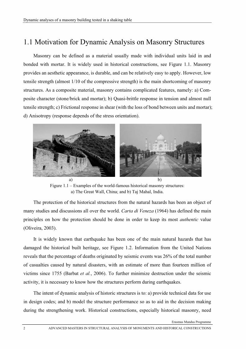
bonded with mortar. It is widely used in historical constructions, see Figure 1.1. Masonry
provides an aesthetic appearance, is durable, and can be relatively easy to apply. However, low
tensile strength (almost 1/10 of the compressive strength) is the main shortcoming of masonry
structures. As a composite material, masonry contains complicated features, namely: a) Com-
posite character (stone/brick and mortar); b) Quasi-brittle response in tension and almost null
tensile strength; c) Frictional response in shear (with the loss of bond between units and mortar);
d) Anisotropy (response depends of the stress orientation).
a) b)
Figure 1.1 – Examples of the world-famous historical masonry structures: a) The Great Wall, China; and b) Taj Mahal, India.
The protection of the historical structures from the natural hazards has been an object of
many studies and discussions all over the world. Carta di Veneza (1964) has defined the main
principles on how the protection should be done in order to keep its most authentic value
(Oliveira, 2003).
It is widely known that earthquake has been one of the main natural hazards that has
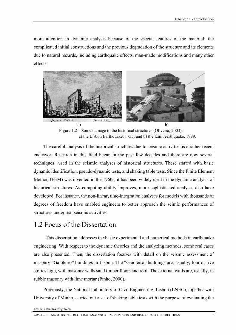
damaged the historical built heritage, see Figure 1.2. Information from the United Nations
reveals that the percentage of deaths originated by seismic events was 26% of the total number
of casualties caused by natural disasters, with an estimate of more than fourteen million of
victims since 1755 (Barbat et al., 2006). To further minimize destruction under the seismic
activity, it is necessary to know how the structures perform during earthquakes.
The intent of dynamic analysis of historic structures is to: a) provide technical data for use
in design codes; and b) model the structure performance so as to aid in the decision making
during the strengthening work. Historical constructions, especially historical masonry, need
Chapter 1 - Introduction
Erasmus Mundus Programme
ADVANCED MASTERS IN STRUCTURAL ANALYSIS OF MONUMENTS AND HISTORICAL CONSTRUCTIONS 3
more attention in dynamic analysis because of the special features of the material; the
complicated initial constructions and the previous degradation of the structure and its elements
due to natural hazards, including earthquake effects, man-made modifications and many other
effects.
a) b) Figure 1.2 – Some damage to the historical structures (Oliveira, 2003):
a) the Lisbon Earthquake, 1755; and b) the Izmit earthquake, 1999.
The careful analysis of the historical structures due to seismic activities is a rather recent
endeavor. Research in this field began in the past few decades and there are now several
techniques used in the seismic analyses of historical structures. These started with basic
dynamic identification, pseudo-dynamic tests, and shaking table tests. Since the Finite Element
Method (FEM) was invented in the 1960s, it has been widely used in the dynamic analysis of
historical structures. As computing ability improves, more sophisticated analyses also have
developed. For instance, the non-linear, time-integration analyses for models with thousands of
degrees of freedom have enabled engineers to better approach the seimic performances of
structures under real seismic activities.
1.2 Focus of the Dissertation
This dissertation addresses the basic experimental and numerical methods in earthquake
engineering. With respect to the dynamic theories and the analyzing methods, some real cases
are also presented. Then, the dissertation focuses with detail on the seismic assessment of
masonry “Gaioleiro” buildings in Lisbon. The “Gaioleiro” buildings are, usually, four or five
stories high, with masonry walls sand timber floors and roof. The external walls are, usually, in
rubble masonry with lime mortar (Pinho, 2000).
Previously, the National Laboratory of Civil Engineering, Lisbon (LNEC), together with
University of Minho, carried out a set of shaking table tests with the purpose of evaluating the
Dynamic analyses of a masonry building tested in a shaking table
Erasmus Mundus Programme
4 ADVANCED MASTERS IN STRUCTURAL ANALYSIS OF MONUMENTS AND HISTORICAL CONSTRUCTIONS
seismic performance of the so called “Gaioleiro” buildings (Candeias et al., 2004). This
dissertation performs numerical modeling using nonlinear time-integration analyses and
compares the results to the data obtained from the previous testing. Furthermore, an updated
full scale numerical model is also analyzed using nonlinear time-integration with the objective
of discussing the effect of the scaling in dynamic analysis.
1.3 Outline of the Dissertation
The dissertation is organized in six chapters by as follows:
Chapter 1 is the introduction of the work, including the motivation, the focus and the
outline of the dissertation;
Chapter 2 presents a state of the art in basic experimental and numerical methods in
earthquake engineering. First, a brief introduction on dynamics is carried out,
followed by a main review of the basic experimental and numerical methods. Issues
about experimental methods addressed include in-situ tests and laboratory tests; then,
issues about numerical methods include time-integration method and pushover
method. Some examples are also discussed in this part;
Chapter 3 presents a description of the prototype, the scaled mock-up and the
numerical model. First, a brief introduction on “Gaioleiro” prototype is provided,
followed by the description of the shaking table tests previously carried out, including
the scaled model, the equipments adopted and the testing procedures. Then the FEM
model is introduced, with the calibration of the numerical model in detail;
Chapter 4 presents an analysis of the experimental and numerical results of the scaled
model. First, for the purpose of optimization, five different numerical models are used
for time-integration analysis, and then compared with the experimental data for 25%
of the Peak Ground Acceleration (PGA). Then, the selected model is used to carry out
100% of the PGA. Aspects considered in the comparisons include: a) the accelerations
and displacements of 80 typical points in four facades; b) the parameters of all the
piers on North/South facades; c) the maximum strain on each facade and crack
patterns. d) the damage factor after the 25% and 100% of the PGA;
Chapter 1 - Introduction
Erasmus Mundus Programme
ADVANCED MASTERS IN STRUCTURAL ANALYSIS OF MONUMENTS AND HISTORICAL CONSTRUCTIONS 5
Chapter 5 addresses the issue of scaling in shaking table tests. As addressed in
Chapter 3, additional masses should have been taken into account in the 1:3 models
tested in the shaking table. Therefore, a calibrated numerical full scale model will be
put into nonlinear time-integration analysis to evaluate the effect of the self weight.
The full scale model is again computationally tested for 25% and 100% PGA, to
compare the new results with the scaled model results. In the end, some conclusions
are provided.
Chapter 6 presents the main conclusions of each chapter and a proposal for future
work.

Dynamic analyses of a masonry building tested in a shaking table
Erasmus Mundus Programme
6 ADVANCED MASTERS IN STRUCTURAL ANALYSIS OF MONUMENTS AND HISTORICAL CONSTRUCTIONS
Chapter 2 – Basic Experimental and Numerical Methods in Earthquake Engineering
Erasmus Mundus Programme
ADVANCED MASTERS IN STRUCTURAL ANALYSIS OF MONUMENTS AND HISTORICAL CONSTRUCTIONS 7
CChhaapptteerr 22
BBaassiicc EExxppeerriimmeennttaall aanndd NNuummeerriiccaall MMeetthhooddss iinn
EEaarrtthhqquuaakkee EEnnggiinneeeerriinngg Abstract In this chapter, a state of the art in basic experimental and numerical methods in earthquake engineering is presented. First, a brief introduction on dynamics is carried out, followed by a main review of the basic experimental and numerical methods. Issues about experimental methods addressed include in-situ tests and laboratory tests; then, issues about numerical methods include time integration method and pushover method. Some examples are also discussed in this part.
Dynamic analyses of a masonry building tested in a shaking table
Erasmus Mundus Programme
8 ADVANCED MASTERS IN STRUCTURAL ANALYSIS OF MONUMENTS AND HISTORICAL CONSTRUCTIONS
2.1 Introduction
The main goal of the present chapter is to review the most important methods in the field
of earthquake engineering. Before presenting the experimental and numerical methods, a brief
introduction on basic dynamics is carried out, aiming to introduce basic concepts and
definitions later mentioned.
2.2 Basic Dynamics
In opposite to static, dynamic can be simply defined as time varying, meaning that a
dynamic load is any load with magnitude, direction, and/or position varying with time.
Similarly, the structural response to a dynamic load, i.e. the resulting stresses and deflections, is
also time varying, or dynamic.
There are two basically different approaches for evaluating the structural response to
dynamic loads: deterministic and nondeterministic. If the time variation of loading is fully
known, even though it may be highly oscillatory or irregular in character, it will be referred to
herein as a prescribed dynamic loading; and the analysis of the response of any specified
structural system to a prescribed dynamic loading is defined as a deterministic analysis. On the
other hand, if the time variation is not completely known but can be defined in a statistical sense,
the loading is termed a random dynamic loading; and its corresponding analysis of response is
defined as a nondeterministic analysis. Generally, structural response to any dynamic loading is
expressed basically in terms of the displacements of the structure. Thus, a deterministic analysis
leads directly to displacement time-histories corresponding to the prescribed loading history;
other related response quantities, such as stresses, strains, internal forces, etc., are usually
obtained as a secondary phase of the analysis (Clough et al., 1995).
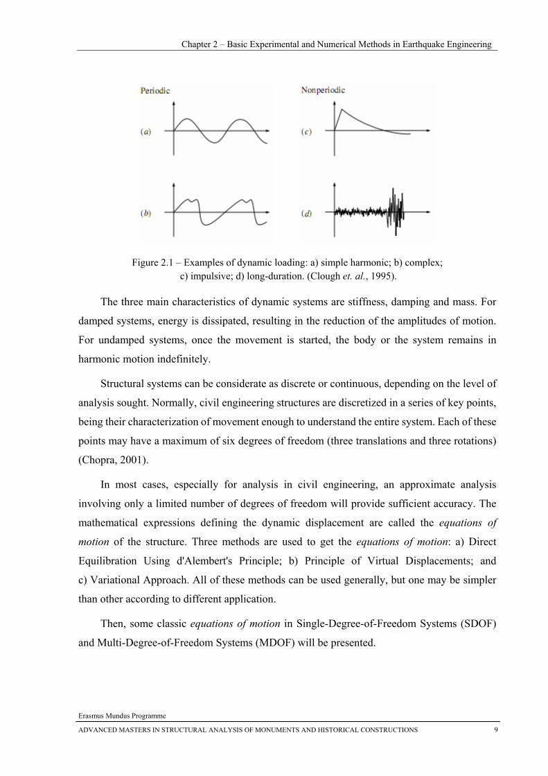
The prescribed loading may be divided into two categories, Periodic and Nonperiodic load.
The simplest periodic loading is shown in Figure 2.1 a, termed simple harmonic; other kind of
periodic loading is more complex with more frequencies, see Figure 2.1 b. Using Fourier
analysis, any periodic loading can be represented as a sum of a series of simple harmonic
components, which can be dealt using in a general procedure. Nonperiodic loadings can be
short-duration impulsive loadings like a blast or explosion, see Figure 2.1 c, or long-duration
general forms of loads like typical earthquake loading, see Figure 2.1 d. Generally,
long-duration loading can be treated only by completely general dynamic analysis procedures.
Chapter 2 – Basic Experimental and Numerical Methods in Earthquake Engineering
Erasmus Mundus Programme
ADVANCED MASTERS IN STRUCTURAL ANALYSIS OF MONUMENTS AND HISTORICAL CONSTRUCTIONS 9
Figure 2.1 – Examples of dynamic loading: a) simple harmonic; b) complex; c) impulsive; d) long-duration. (Clough et. al., 1995).
The three main characteristics of dynamic systems are stiffness, damping and mass. For
damped systems, energy is dissipated, resulting in the reduction of the amplitudes of motion.
For undamped systems, once the movement is started, the body or the system remains in
harmonic motion indefinitely.
Structural systems can be considerate as discrete or continuous, depending on the level of
analysis sought. Normally, civil engineering structures are discretized in a series of key points,
being their characterization of movement enough to understand the entire system. Each of these
points may have a maximum of six degrees of freedom (three translations and three rotations)
(Chopra, 2001).
In most cases, especially for analysis in civil engineering, an approximate analysis
involving only a limited number of degrees of freedom will provide sufficient accuracy. The
mathematical expressions defining the dynamic displacement are called the equations of
motion of the structure. Three methods are used to get the equations of motion: a) Direct
Equilibration Using d'Alembert's Principle; b) Principle of Virtual Displacements; and
c) Variational Approach. All of these methods can be used generally, but one may be simpler
than other according to different application.
Then, some classic equations of motion in Single-Degree-of-Freedom Systems (SDOF)
and Multi-Degree-of-Freedom Systems (MDOF) will be presented.
Dynamic analyses of a masonry building tested in a shaking table
Erasmus Mundus Programme
10 ADVANCED MASTERS IN STRUCTURAL ANALYSIS OF MONUMENTS AND HISTORICAL CONSTRUCTIONS
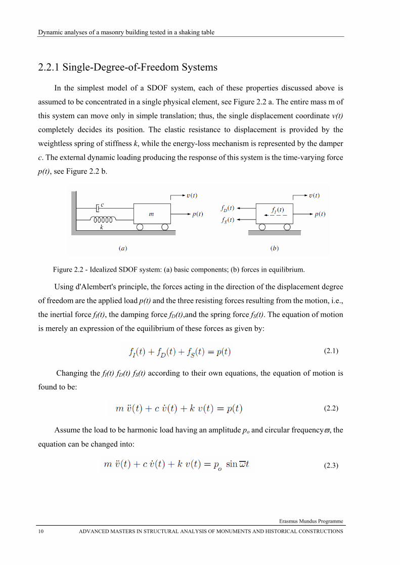
2.2.1 Single-Degree-of-Freedom Systems
In the simplest model of a SDOF system, each of these properties discussed above is
assumed to be concentrated in a single physical element, see Figure 2.2 a. The entire mass m of
this system can move only in simple translation; thus, the single displacement coordinate v(t)
completely decides its position. The elastic resistance to displacement is provided by the
weightless spring of stiffness k, while the energy-loss mechanism is represented by the damper
c. The external dynamic loading producing the response of this system is the time-varying force
p(t), see Figure 2.2 b.
Figure 2.2 - Idealized SDOF system: (a) basic components; (b) forces in equilibrium.
Using d'Alembert's principle, the forces acting in the direction of the displacement degree
of freedom are the applied load p(t) and the three resisting forces resulting from the motion, i.e.,
the inertial force fI(t), the damping force fD(t),and the spring force fS(t). The equation of motion
is merely an expression of the equilibrium of these forces as given by:
(2.1)
Changing the fI(t) fD(t) fS(t) according to their own equations, the equation of motion is
found to be:
(2.2)
Assume the load to be harmonic load having an amplitude po and circular frequencyϖ, the
equation can be changed into:
(2.3)
Chapter 2 – Basic Experimental and Numerical Methods in Earthquake Engineering
Erasmus Mundus Programme
ADVANCED MASTERS IN STRUCTURAL ANALYSIS OF MONUMENTS AND HISTORICAL CONSTRUCTIONS 11
A straightforward mathematical process provides the response of system under harmonic
load, found as:
(2.4)
Here, A, B depend on the initial conditions: initial displacement v(t) and initial velocity
v’(t) , given by:
(2.5)
(2.6)
and ξ is the damping ratio:
(2.7)
For an arbitrary force acting in the system, the solution of this second order differential
equation can be obtained by the Duhamel’s integral (Chopra, 2001), valid for linear systems
and given by the following expression, in which q(t) is equal to v(t) in equation (2.2):
(2.8)
2.2.2 Multi-Degree-of-Freedom Systems
The equation of motion of the system of a MDOF system can be formulated by expressing
the equilibrium of the effective forces associated with each of its degrees of freedom. So the
general expression can be made in matrix form:
(2.9) where k, c, m are defied as stiffness matrix, damping matrix and mass matrix:
(2.10)
(2.11)
(2.12)
Thus, Equation (2.9) can be changed into:
(2.13)
Dynamic analyses of a masonry building tested in a shaking table
Erasmus Mundus Programme
12 ADVANCED MASTERS IN STRUCTURAL ANALYSIS OF MONUMENTS AND HISTORICAL CONSTRUCTIONS
Then the concepts of eigenvalue or characteristic value problems are required. For a freely
vibrating undamped system MDOF system, the equations of motion can be obtained by
omitting the damping matrix c:
(2.14)
Let :
(2.15)
and the following equation can be obtained as:
(2.16)
The solution of Equation (2.16) will be the eigenvalue vector ω , see Equation (2.17) and
matrix in Equation (2.18) provides the mode shape vectors for the free vibration.
(2.17)
(2.18)
The displacement vector v may be also expressed by summing the modal vectors as:
(2.19)
So the equation of motion can be obtained as:
(2.20)
and the Duhamel integral will be given by:
(2.21)
Chapter 2 – Basic Experimental and Numerical Methods in Earthquake Engineering
Erasmus Mundus Programme
ADVANCED MASTERS IN STRUCTURAL ANALYSIS OF MONUMENTS AND HISTORICAL CONSTRUCTIONS 13
2.3 Experimental Methods
In the previous section, some basic reviews of the basic dynamics were presented in order
to better understand the experimental methods and numerical methods later addressed. As
referred, for the equation of motion of any system, three main characteristics are stiffness,
damping and mass. The object of the simplest dynamic testing is to measuring these dynamic
characteristics of the structures, however, the purposes of the experimental methods of the
dynamic analysis of historical structures now has been spreaded for: a) assessment of safety and
definition of reliability; b) understanding existing damage; c) the evaluation of strengthening
and/or repair efficiency; d) measuring dynamic characteristics of buildings, e.g. natural
frequencies, damping values, hysteretic response.
In short, dynamic testing can be used to obtain modal characterization, but also to check
and evaluate the statistical parameters of the recorded response signals, supplying quantitative
information. The influence factors, the properties and the response involved in structural
dynamic tests are provided in Figure 2.3 .
Figure 2.3 – Influence, properties and response involved in structural dynamic tests.
Dynamic analyses of a masonry building tested in a shaking table
Erasmus Mundus Programme
14 ADVANCED MASTERS IN STRUCTURAL ANALYSIS OF MONUMENTS AND HISTORICAL CONSTRUCTIONS
2.3.1 In-situ Vibration Tests
Vibration testing is now a mature and widely used tool in the analysis of structural systems,
as a non-destructive test that can be valuable for historic structures. Vibration tests on historic
buildings might have the following goals: a) understand how the structure behaves; b) find
when a damage failure threshold occurs; c) locate damage in the structure.
Typically two types of vibration tests may be applied: sinusoidal and random. The
sinusoidal test consists of a certain acceleration level (amplitude, energy output) combined with
a frequency sweep at a range from an initial frequency to a final frequency. The sinusoidal tests
can illustrate the resonant frequencies of the structure and allow often an easy mathematical
treatment. A structure in a random vibration test is exposed to energies at all frequencies in the
bandwidth selected and the analysis requires a statistical description (Pospíšil, 2002)
Before presenting the vibration tests, some basic introduction of the dynamic
identification are made.
2.2.3.1 Basic Dynamic Identification Method
The purpose of dynamic identification is to identify structural damage and deterioration
according to the measured modal parameters. The conventional modal identifications is based
on structural response induced by known excitation such as a simple harmonic vibration
imposed by an artificial excitation. The structural parameters are identified either from the free
vibration decay traces, after the excitation is removed, or simply as a transfer function between
input and output of the system.
Various techniques have been developed to determine the structural parameters. The basic
idea is to assume mathematical models for the system and then to minimize the prediction
errors by fitting the models against the obtained output data.
In what concerns in situ modal identification tests there are two groups of experimental
techniques: (a) the input-output vibration tests, where the excitation forces and the vibration
response are measured; (b) the output-only tests, where only the response of the system is
measured (from ambient vibration or from the free vibration tests, where an initial deformation
and then are quickly released).
Chapter 2 – Basic Experimental and Numerical Methods in Earthquake Engineering
Erasmus Mundus Programme
ADVANCED MASTERS IN STRUCTURAL ANALYSIS OF MONUMENTS AND HISTORICAL CONSTRUCTIONS 15
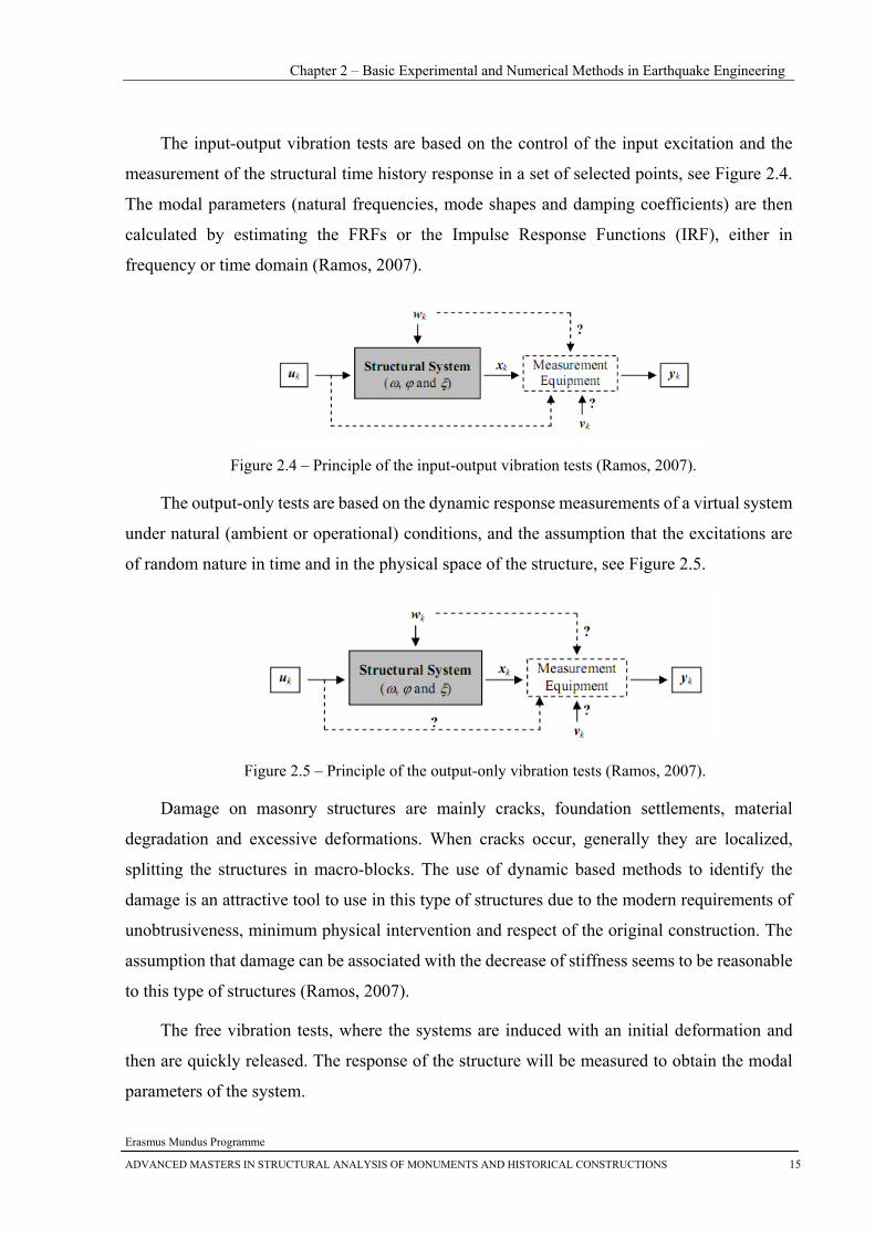
The input-output vibration tests are based on the control of the input excitation and the
measurement of the structural time history response in a set of selected points, see Figure 2.4.
The modal parameters (natural frequencies, mode shapes and damping coefficients) are then
calculated by estimating the FRFs or the Impulse Response Functions (IRF), either in
frequency or time domain (Ramos, 2007).
Figure 2.4 – Principle of the input-output vibration tests (Ramos, 2007).
The output-only tests are based on the dynamic response measurements of a virtual system
under natural (ambient or operational) conditions, and the assumption that the excitations are
of random nature in time and in the physical space of the structure, see Figure 2.5.
Figure 2.5 – Principle of the output-only vibration tests (Ramos, 2007).
Damage on masonry structures are mainly cracks, foundation settlements, material
degradation and excessive deformations. When cracks occur, generally they are localized,
splitting the structures in macro-blocks. The use of dynamic based methods to identify the
damage is an attractive tool to use in this type of structures due to the modern requirements of
unobtrusiveness, minimum physical intervention and respect of the original construction. The
assumption that damage can be associated with the decrease of stiffness seems to be reasonable
to this type of structures (Ramos, 2007).
The free vibration tests, where the systems are induced with an initial deformation and
then are quickly released. The response of the structure will be measured to obtain the modal
parameters of the system.
Dynamic analyses of a masonry building tested in a shaking table
Erasmus Mundus Programme
16 ADVANCED MASTERS IN STRUCTURAL ANALYSIS OF MONUMENTS AND HISTORICAL CONSTRUCTIONS
2.2.3.2 Description of In-situ Vibration Tests
Vibration testing requires the following successive tasks: acquisition of data with a
sensing system; communication of the information gathered; intelligent processing and
analyzing of data; storage of processed data; diagnostics (e.g. damage detection or comparison
with numerical simulation).
Generally, an irregular or unexpected property of the dynamic response can reveal a
“symptom” of structural weakness. The presence of several symptoms might make a direct and
deterministic interpretation difficult, meaning that “pattern recognition” or artificial
intelligence techniques may be effective. Alternative methods are those founded on updating
numerical models: model correction is based on the results of a previous structural
identification (model updating techniques).
2.2.3.3 Examples of In-situ Vibration Tests
Selected examples of in situ vibration tests are briefly described next, to illustrate how
these techniques are applied to cultural heritage buildings:
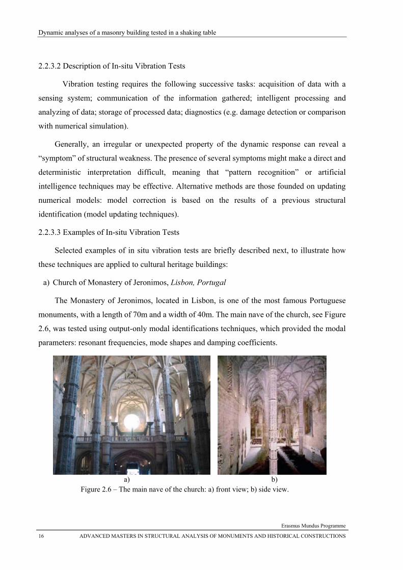
a) Church of Monastery of Jeronimos, Lisbon, Portugal
The Monastery of Jeronimos, located in Lisbon, is one of the most famous Portuguese
monuments, with a length of 70m and a width of 40m. The main nave of the church, see Figure
2.6, was tested using output-only modal identifications techniques, which provided the modal
parameters: resonant frequencies, mode shapes and damping coefficients.
a) b)
Figure 2.6 – The main nave of the church: a) front view; b) side view.
Chapter 2 – Basic Experimental and Numerical Methods in Earthquake Engineering
Erasmus Mundus Programme
ADVANCED MASTERS IN STRUCTURAL ANALYSIS OF MONUMENTS AND HISTORICAL CONSTRUCTIONS 17
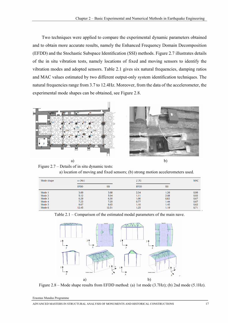
Two techniques were applied to compare the experimental dynamic parameters obtained
and to obtain more accurate results, namely the Enhanced Frequency Domain Decomposition
(EFDD) and the Stochastic Subspace Identification (SSI) methods. Figure 2.7 illustrates details
of the in situ vibration tests, namely locations of fixed and moving sensors to identify the
vibration modes and adopted sensors. Table 2.1 gives six natural frequencies, damping ratios
and MAC values estimated by two different output-only system identification techniques. The
natural frequencies range from 3.7 to 12.4Hz. Moreover, from the data of the accelerometer, the
experimental mode shapes can be obtained, see Figure 2.8.
a) b)
Figure 2.7 – Details of in situ dynamic tests: a) location of moving and fixed sensors; (b) strong motion accelerometers used.
Table 2.1 – Comparison of the estimated modal parameters of the main nave.
a) b)
Figure 2.8 – Mode shape results from EFDD method: (a) 1st mode (3.7Hz); (b) 2nd mode (5.1Hz).
Dynamic analyses of a masonry building tested in a shaking table
Erasmus Mundus Programme
18 ADVANCED MASTERS IN STRUCTURAL ANALYSIS OF MONUMENTS AND HISTORICAL CONSTRUCTIONS
As shown in Table 2.1, MAC values are calculated for the eight mode shape vectors
obtained from two experimental techniques. The MAC criterion is the most well known
procedure to study the correlation between to sets of mode shape vectors. The results vary
from 0 to 1, i.e. from bad to good correlation. Observing the table values, the two first mode
shapes are highly correlated (values closed to the unit), but for the rest of the modes the values
decreases, to a minimum of 0.36.
Nevertheless, the modal identification seems to be acceptable if the structural complexity
of the main nave is taken into consideration. Even if the mode shape and damping coefficients
estimation is not very accurate for the higher modes, the resonant frequencies were accurately
calculated by the two experimental techniques for all estimated modes. (Ramos and Lourenço,
2005)
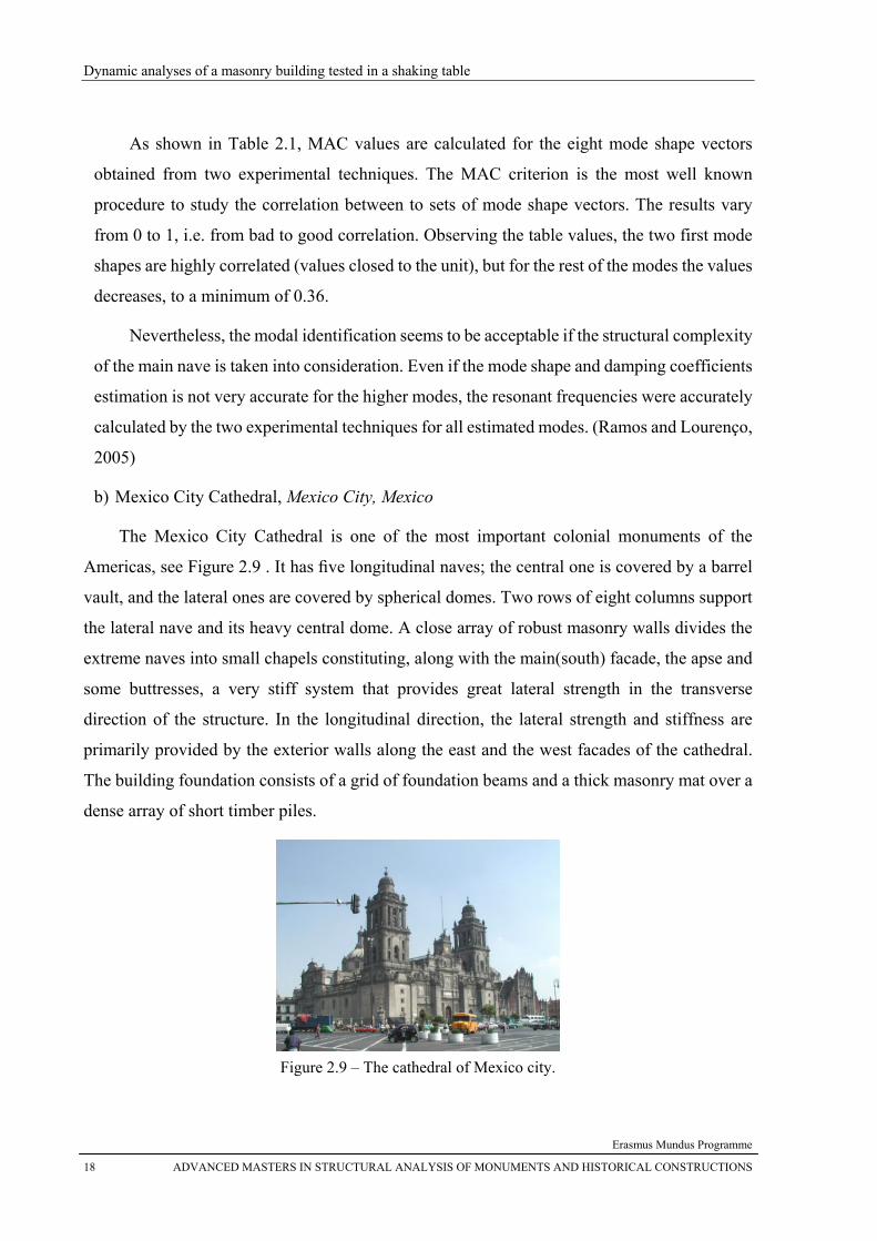
b) Mexico City Cathedral, Mexico City, Mexico
The Mexico City Cathedral is one of the most important colonial monuments of the
Americas, see Figure 2.9 . It has five longitudinal naves; the central one is covered by a barrel
vault, and the lateral ones are covered by spherical domes. Two rows of eight columns support
the lateral nave and its heavy central dome. A close array of robust masonry walls divides the
extreme naves into small chapels constituting, along with the main(south) facade, the apse and
some buttresses, a very stiff system that provides great lateral strength in the transverse
direction of the structure. In the longitudinal direction, the lateral strength and stiffness are
primarily provided by the exterior walls along the east and the west facades of the cathedral.
The building foundation consists of a grid of foundation beams and a thick masonry mat over a
dense array of short timber piles.
Figure 2.9 – The cathedral of Mexico city.
Chapter 2 – Basic Experimental and Numerical Methods in Earthquake Engineering
Erasmus Mundus Programme
ADVANCED MASTERS IN STRUCTURAL ANALYSIS OF MONUMENTS AND HISTORICAL CONSTRUCTIONS 19
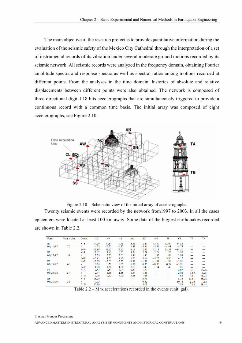
The main objective of the research project is to provide quantitative information during the
evaluation of the seismic safety of the Mexico City Cathedral through the interpretation of a set
of instrumental records of its vibration under several moderate ground motions recorded by its
seismic network. All seismic records were analyzed in the frequency domain, obtaining Fourier
amplitude spectra and response spectra as well as spectral ratios among motions recorded at
different points. From the analyses in the time domain, histories of absolute and relative
displacements between different points were also obtained. The network is composed of
three-directional digital 18 bits accelerographs that are simultaneously triggered to provide a
continuous record with a common time basis. The initial array was composed of eight
accelerographs, see Figure 2.10.
Figure 2.10 – Schematic view of the initial array of accelerographs. Twenty seismic events were recorded by the network from1997 to 2003. In all the cases
epicenters were located at least 100 km away. Some data of the biggest earthquakes recorded
are shown in Table 2.2.
Table 2.2 – Max accelerations recorded in the events (unit: gal).
Dynamic analyses of a masonry building tested in a shaking table
Erasmus Mundus Programme
20 ADVANCED MASTERS IN STRUCTURAL ANALYSIS OF MONUMENTS AND HISTORICAL CONSTRUCTIONS
For engineering purposes, characteristics of the seismic ground motion are usually studied
through acceleration response spectra for 5% damping. A set of these spectra is shown in Figure
2.11 a, for the N-S direction at the ‘free-field’ station. It can be seen that spectral shapes change
with earthquake magnitude, and the earthquakes of highest intensity show a significant
amplification of response for long periods. This is attributed to the higher content of long period
waves in large magnitude earthquakes compared with that in moderate magnitude events.
a) b)
Figure 2.11 – Results in N-S direction: a) Acceleration response spectra; (b) the ratio of Fourier spectral amplitudes.
To better identify site effects, spectral ratios of the Fourier spectral amplitudes were
obtained between the cathedral site and a station located on firm ground in Mexico City, where
the same events were recorded (CU station). These functions, shown in Figure 2.11 b, for the
five most significant events and for N-S direction, allow one to clearly identify the first mode of
vibration of the soil deposits at the site, at approximately 0.37 Hz for the N–S direction. The
seismic network installed at the cathedral has been successful in terms of the number and
quality of records gathered in a limited time span and of the knowledge derived from them
(Riveral and Meli et al., 2008).
2.3.2 Laboratory Dynamic Tests
In the previous section, the in-situ vibration tests were presented. For the in-situ tests, the
purposes are normally evaluating the safety, monitoring the health and analyzing for the
strengthening. For the purpose of achieving the further, and more accurate, information on
seismic behavior of historical structures, laboratory dynamic tests are necessary. In the
following section, two basic laboratory dynamic tests are presented.
Chapter 2 – Basic Experimental and Numerical Methods in Earthquake Engineering
Erasmus Mundus Programme
ADVANCED MASTERS IN STRUCTURAL ANALYSIS OF MONUMENTS AND HISTORICAL CONSTRUCTIONS 21
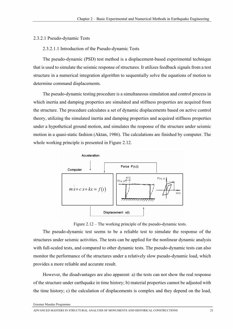
2.3.2.1 Pseudo-dynamic Tests
2.3.2.1.1 Introduction of the Pseudo-dynamic Tests
The pseudo-dynamic (PSD) test method is a displacement-based experimental technique
that is used to simulate the seismic response of structures. It utilizes feedback signals from a test
structure in a numerical integration algorithm to sequentially solve the equations of motion to
determine command displacements.
The pseudo-dynamic testing procedure is a simultaneous simulation and control process in
which inertia and damping properties are simulated and stiffness properties are acquired from
the structure. The procedure calculates a set of dynamic displacements based on active control
theory, utilizing the simulated inertia and damping properties and acquired stiffness properties
under a hypothetical ground motion, and simulates the response of the structure under seismic
motion in a quasi-static fashion (Aktan, 1986). The calculations are finished by computer. The
whole working principle is presented in Figure 2.12.
Figure 2.12 – The working principle of the pseudo-dynamic tests.
The pseudo-dynamic test seems to be a reliable test to simulate the response of the
structures under seismic activities. The tests can be applied for the nonlinear dynamic analysis
with full-scaled tests, and compared to other dynamic tests. The pseudo-dynamic tests can also
monitor the performance of the structures under a relatively slow pseudo-dynamic load, which
provides a more reliable and accurate result.
However, the disadvantages are also apparent: a) the tests can not show the real response
of the structure under earthquake in time history; b) material properties cannot be adjusted with
the time history; c) the calculation of displacements is complex and they depend on the load,
Dynamic analyses of a masonry building tested in a shaking table
Erasmus Mundus Programme
22 ADVANCED MASTERS IN STRUCTURAL ANALYSIS OF MONUMENTS AND HISTORICAL CONSTRUCTIONS
meaning that the accuracy is hard to control; d) the load is applied in certain locations, and so
the method can only be applied on the simplified mass concentration structure (MDOF); e) the
tests also has high requirements of the equipments, and it is usually rather costly.
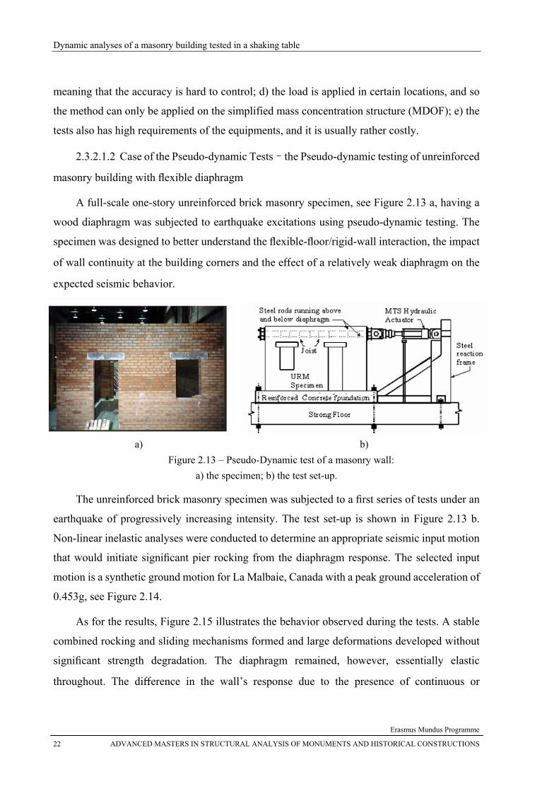
2.3.2.1.2 Case of the Pseudo-dynamic Tests–the Pseudo-dynamic testing of unreinforced
masonry building with flexible diaphragm
A full-scale one-story unreinforced brick masonry specimen, see Figure 2.13 a, having a
wood diaphragm was subjected to earthquake excitations using pseudo-dynamic testing. The
specimen was designed to better understand the flexible-floor/rigid-wall interaction, the impact
of wall continuity at the building corners and the effect of a relatively weak diaphragm on the
expected seismic behavior.
a) b)
Figure 2.13 – Pseudo-Dynamic test of a masonry wall: a) the specimen; b) the test set-up.
The unreinforced brick masonry specimen was subjected to a first series of tests under an
earthquake of progressively increasing intensity. The test set-up is shown in Figure 2.13 b.
Non-linear inelastic analyses were conducted to determine an appropriate seismic input motion
that would initiate significant pier rocking from the diaphragm response. The selected input
motion is a synthetic ground motion for La Malbaie, Canada with a peak ground acceleration of
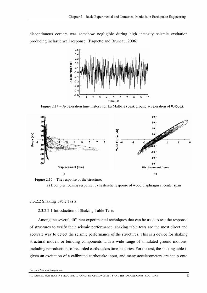
0.453g, see Figure 2.14.
As for the results, Figure 2.15 illustrates the behavior observed during the tests. A stable
combined rocking and sliding mechanisms formed and large deformations developed without
significant strength degradation. The diaphragm remained, however, essentially elastic
throughout. The difference in the wall’s response due to the presence of continuous or
Chapter 2 – Basic Experimental and Numerical Methods in Earthquake Engineering
Erasmus Mundus Programme
ADVANCED MASTERS IN STRUCTURAL ANALYSIS OF MONUMENTS AND HISTORICAL CONSTRUCTIONS 23
discontinuous corners was somehow negligible during high intensity seismic excitation
producing inelastic wall response. (Paquette and Bruneau, 2006)
Figure 2.14 –.Acceleration time history for La Malbaie (peak ground acceleration of 0.453g).
a) b) Figure 2.15 – The response of the structure: a) Door pier rocking response; b) hysteretic response of wood diaphragm at center span
2.3.2.2 Shaking Table Tests
2.3.2.2.1 Introduction of Shaking Table Tests
Among the several different experimental techniques that can be used to test the response
of structures to verify their seismic performance, shaking table tests are the most direct and
accurate way to detect the seismic performance of the structures. This is a device for shaking
structural models or building components with a wide range of simulated ground motions,
including reproductions of recorded earthquakes time-histories. For the test, the shaking table is
given an excitation of a calibrated earthquake input, and many accelerometers are setup onto
Dynamic analyses of a masonry building tested in a shaking table
Erasmus Mundus Programme
24 ADVANCED MASTERS IN STRUCTURAL ANALYSIS OF MONUMENTS AND HISTORICAL CONSTRUCTIONS
the structures to obtain the data of the response during the dynamic loading. After analyzing the
data of the accelerometer, the general parameters of response can be obtained and analyzed
furthermore. While modern tables typically consist of a rectangular platform that is driven in up
to six degrees of freedom (DOF) by servo-hydraulic or other types of actuators, the earliest
reported uses of shake tables date back more than a century (Omori, 1900).
Generally, test specimens are fixed to the platform and shaken, often adding load to the
point of failure. Using video cameras and data from transducers, accelerometers normally, it is
possible to interpret the dynamic behaviors of the specimen. Shaking table tests are used
extensively in seismic research, as they provide the ways to excite structures in such a way that
the structures are subjected to conditions representative of true earthquake ground motions. .
Shaking table tests results are also the main way used in this dissertation and will be
presented in detail in the following chapters. To better understand the tests, an example of a real
case is introduced here.
2.3.2.2.2 Case of Shaking Table Tests
In many European countries like France, Greece, Italy, Portugal, Romania, Slovakia and
Spain there is a good tradition for using natural stone masonry in buildings and structures. They
are long lasting constructions very convenient in severe conditions of climate and foundations.
Stone masonry can be used either partially for foundation and first storey walls or for the whole
structure, being the high cost of labor, the most limiting condition for their use during the last
decades. Recently, rapid rising of energy costs and increasing of losses due to natural
catastrophes draw back the attention to natural stone masonry. Originally, stone masonry was
made with lime mortar that, despite its low tensile resistance, presents a considerable ductility
that contributes to reduce the effects of stress concentration. For improving the general
characteristics of the stone masonry constructions, including their response to seismic actions,
strengthening the masonry structural members with polymer grids were studied with shaking
table tests.
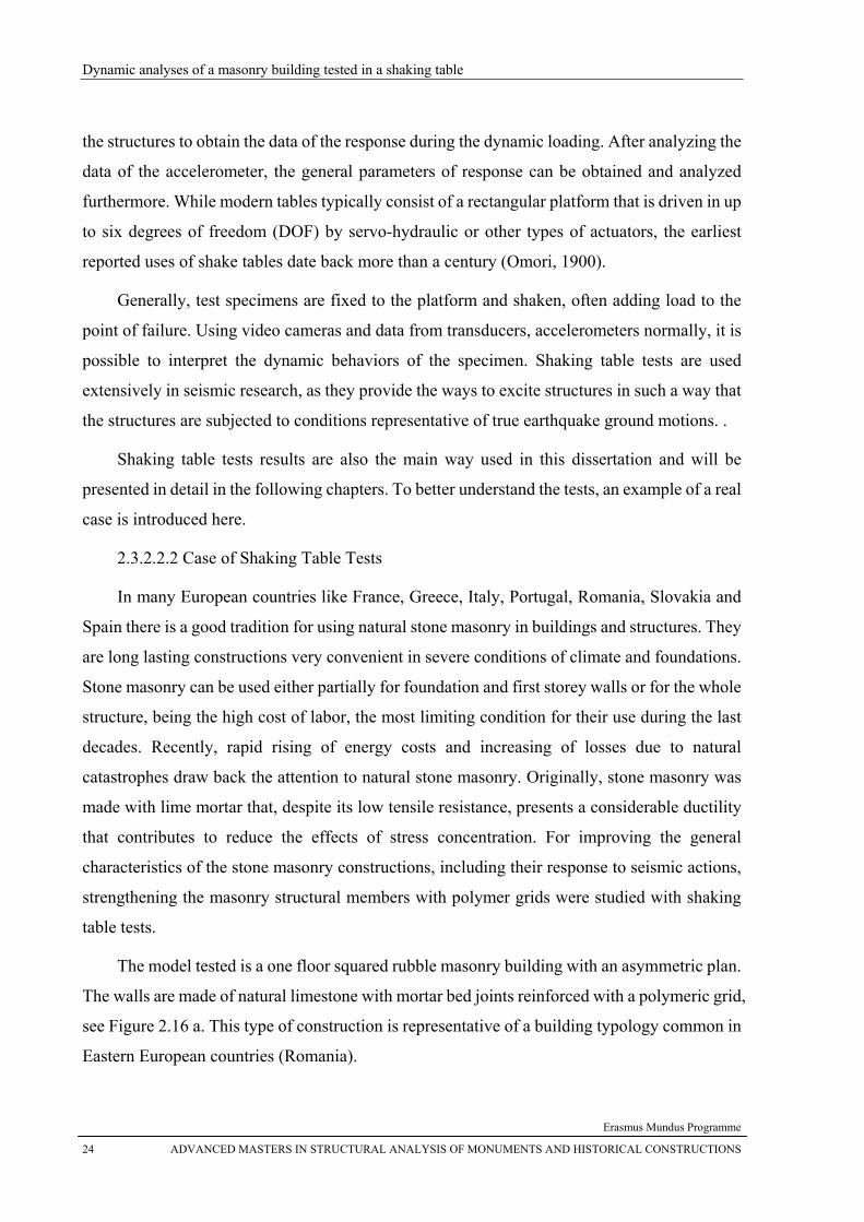
The model tested is a one floor squared rubble masonry building with an asymmetric plan.
The walls are made of natural limestone with mortar bed joints reinforced with a polymeric grid,
see Figure 2.16 a. This type of construction is representative of a building typology common in
Eastern European countries (Romania).
Chapter 2 – Basic Experimental and Numerical Methods in Earthquake Engineering
Erasmus Mundus Programme
ADVANCED MASTERS IN STRUCTURAL ANALYSIS OF MONUMENTS AND HISTORICAL CONSTRUCTIONS 25
a) b)
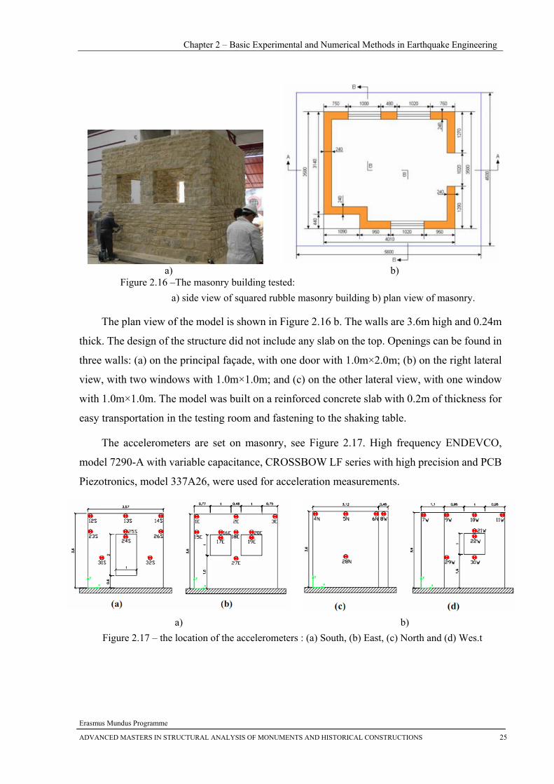
Figure 2.16 –The masonry building tested: a) side view of squared rubble masonry building b) plan view of masonry.
The plan view of the model is shown in Figure 2.16 b. The walls are 3.6m high and 0.24m
thick. The design of the structure did not include any slab on the top. Openings can be found in
three walls: (a) on the principal façade, with one door with 1.0m×2.0m; (b) on the right lateral
view, with two windows with 1.0m×1.0m; and (c) on the other lateral view, with one window
with 1.0m×1.0m. The model was built on a reinforced concrete slab with 0.2m of thickness for
easy transportation in the testing room and fastening to the shaking table.
The accelerometers are set on masonry, see Figure 2.17. High frequency ENDEVCO,
model 7290-A with variable capacitance, CROSSBOW LF series with high precision and PCB
Piezotronics, model 337A26, were used for acceleration measurements.
a) b) Figure 2.17 – the location of the accelerometers : (a) South, (b) East, (c) North and (d) Wes.t
Dynamic analyses of a masonry building tested in a shaking table
Erasmus Mundus Programme
26 ADVANCED MASTERS IN STRUCTURAL ANALYSIS OF MONUMENTS AND HISTORICAL CONSTRUCTIONS
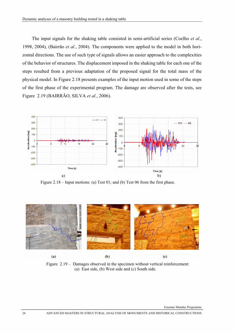
The input signals for the shaking table consisted in semi-artificial series (Coelho et al.,
1998, 2004), (Bairrão et al., 2004). The components were applied to the model in both hori-
zontal directions. The use of such type of signals allows an easier approach to the complexities
of the behavior of structures. The displacement imposed in the shaking table for each one of the
steps resulted from a previous adaptation of the proposed signal for the total mass of the
physical model. In Figure 2.18 presents examples of the input motion used in some of the steps
of the first phase of the experimental program. The damage are observed after the tests, see
Figure 2.19 (BAIRRÃO, SILVA et al., 2006).
a) b)
Figure 2.18 – Input motions: (a) Test 01; and (b) Test 06 from the first phase.
Figure 2.19 – Damages observed in the specimen without vertical reinforcement:
(a) East side, (b) West side and (c) South side.
Chapter 2 – Basic Experimental and Numerical Methods in Earthquake Engineering
Erasmus Mundus Programme
ADVANCED MASTERS IN STRUCTURAL ANALYSIS OF MONUMENTS AND HISTORICAL CONSTRUCTIONS 27
2.4 Numerical Methods
For analyzing the dynamic response of the structure in numerical methods, two means are
normally used: Step-by-step Analysis (Time Integration Analysis) and Pushover Analysis. The
Step-by-step Analysis or so called Time Integration Analysis is a classic approach of the time
domain analysis, which can accurately represent the response of the structure at any given time.
And this way can be also conveniently used in the nonlinear analysis (Material Nonlinear or
Geographic Nonlinear), because the properties can be updated anytime during the calculation.
In order to get stable results, the time steps (time intervals) must be small enough, which causes
a large processing time. Thus the analysis is accurate but quite time-consuming. A static
procedure is often adopted to overcome this. Pushover analysis has been proved to be a reliable
way to analysis the response of the structure, especially during large earthquakes, particularly
to test the locations of plastic hinges and the ultimate capacity of the structure (Chopra, 1999).
Pushover analysis is also recommended in many codes, as an adequate tool for the seismic
safety evaluation of structures.
Next, these two methods will be briefly presented.
2.4.1 Time Integration Analysis
The step-by-step procedure is a general approach to dynamic response analysis, and it is
well suited to analysis of nonlinear response because it avoids any use of superposition.
2.4.1.1 Description of the Time Integration Analysis
There are many different step-by-step methods, but in all of them the loading and the
response history are divided into a sequence of time intervals or “steps”. The response during
each step then is calculated from the initial conditions (displacement and velocity) existing at
the beginning of the step and from the history of loading during the step. Thus the response for
each step is an independent analysis problem, and there is no need to combine response
contributions within the step.
Nonlinear behavior may be considered easily by this approach merely by assuming that
the structural properties remain constant during each step and causing them to change in
accordance with any specified form of behavior from one step to the next; hence the nonlinear
analysis actually is a sequence of linear analyses of a changing system. Any desired degree of
Dynamic analyses of a masonry building tested in a shaking table
Erasmus Mundus Programme
28 ADVANCED MASTERS IN STRUCTURAL ANALYSIS OF MONUMENTS AND HISTORICAL CONSTRUCTIONS
refinement in the nonlinear behavior may be achieved in this procedure by making the time
steps short enough; also it can be applied to any type of nonlinearity, including changes of mass
and damping properties as well as the more common nonlinearities due to changes of stiffness.
Step-by-step methods provide the only completely general approach to analysis of
nonlinear response; however, the methods are equally valuable in the analysis of linear
response because the same algorithms can be applied regardless of whether the structure is
behaving linearly or not. Moreover, the procedures used in solving (SDOF) systems can easily
be extended to deal with MDOF systems merely by replacing scalar quantities by matrices. In
fact, these methods are so effective and convenient that time-domain analyses almost always
are done by some form of step-by-step analysis regardless of whether the response behavior is
linear; the Duhamel integral method seldom is used in practice. (Clough, 1995)
2.4.1.2 Numerical Approximation Procedures of the Method
The simplest step-by-step method for analysis of SDOF systems is the so-called
“piecewise exact method”, which is based on the exact solution of the equation of motion for
response of a linear structure to a loading that varies linearly during a discrete time interval. But
here attention will be focused on the MDOF system and the Numerical Approximation
Procedures relatively. (Chopra, 2001)
The step-by-step methods employ numerical procedures to approximately satisfy the
equations of motion during each time step - using either numerical differentiation or numerical
integration. Taking the most common approach, Newmark-β Method, as an example, some
aspects will be reviewed next.
A general step-by-step formulation was proposed by Newmark, which includes the
preceding method as a special case, but also may be applied in several other versions.
Equations of motion for a linear MDOF system excited by force vector p(t) or
earthquake-induced ground motion are given by:
(2.22)
Here, the time scale is divided into a series of time steps, usually of constant duration.
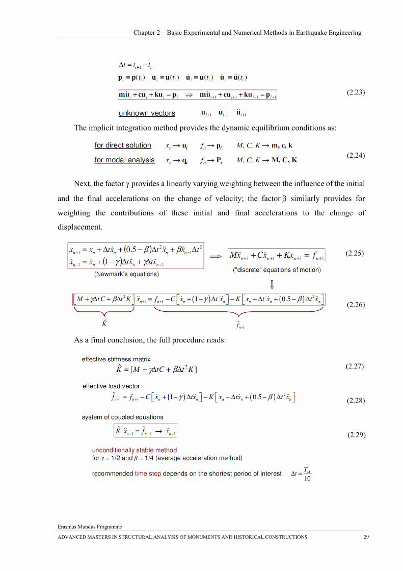
Chapter 2 – Basic Experimental and Numerical Methods in Earthquake Engineering
Erasmus Mundus Programme
ADVANCED MASTERS IN STRUCTURAL ANALYSIS OF MONUMENTS AND HISTORICAL CONSTRUCTIONS 29
(2.23)
The implicit integration method provides the dynamic equilibrium conditions as:
(2.24)
Next, the factor γ provides a linearly varying weighting between the influence of the initial
and the final accelerations on the change of velocity; the factor β similarly provides for
weighting the contributions of these initial and final accelerations to the change of
displacement.
(2.25)
(2.26)
As a final conclusion, the full procedure reads:
(2.27)
(2.28)
(2.29)
Dynamic analyses of a masonry building tested in a shaking table
Erasmus Mundus Programme
30 ADVANCED MASTERS IN STRUCTURAL ANALYSIS OF MONUMENTS AND HISTORICAL CONSTRUCTIONS
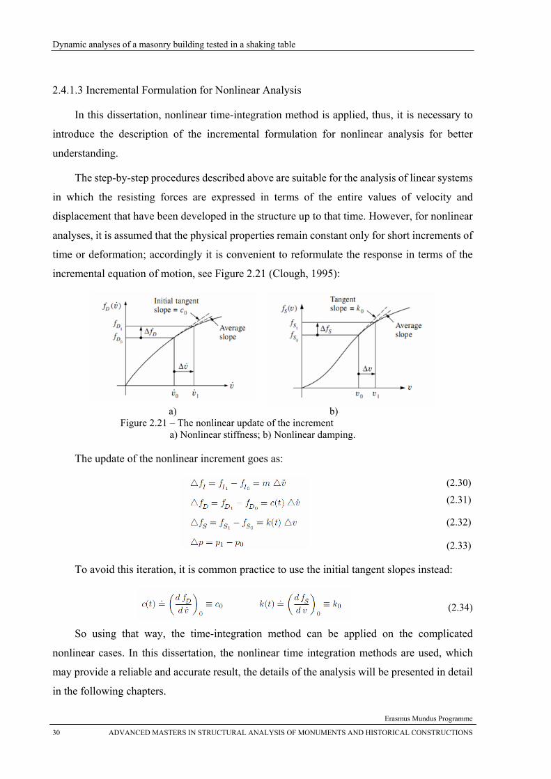
2.4.1.3 Incremental Formulation for Nonlinear Analysis
In this dissertation, nonlinear time-integration method is applied, thus, it is necessary to
introduce the description of the incremental formulation for nonlinear analysis for better
understanding.
The step-by-step procedures described above are suitable for the analysis of linear systems
in which the resisting forces are expressed in terms of the entire values of velocity and
displacement that have been developed in the structure up to that time. However, for nonlinear
analyses, it is assumed that the physical properties remain constant only for short increments of
time or deformation; accordingly it is convenient to reformulate the response in terms of the
incremental equation of motion, see Figure 2.21 (Clough, 1995):
a) b)
Figure 2.21 – The nonlinear update of the increment a) Nonlinear stiffness; b) Nonlinear damping.
The update of the nonlinear increment goes as:
(2.30)
(2.31)
(2.32)
(2.33)
To avoid this iteration, it is common practice to use the initial tangent slopes instead:
(2.34)
So using that way, the time-integration method can be applied on the complicated
nonlinear cases. In this dissertation, the nonlinear time integration methods are used, which
may provide a reliable and accurate result, the details of the analysis will be presented in detail
in the following chapters.
Chapter 2 – Basic Experimental and Numerical Methods in Earthquake Engineering
Erasmus Mundus Programme
ADVANCED MASTERS IN STRUCTURAL ANALYSIS OF MONUMENTS AND HISTORICAL CONSTRUCTIONS 31
2.4.2 Pushover Analysis
The recent advent of performance based design has brought the nonlinear static pushover
analysis procedure to the forefront. Pushover analysis is a static, nonlinear procedure in which
the magnitude of the structural loading is incrementally increased in accordance with a certain
predefined pattern. With the increase in the magnitude of the loading, weak links and failure
modes of the structure are found. The loading is monotonic with the effects of the cyclic
behavior and load reversals being estimated by using a modified monotonic force-deformation
criteria and with damping approximations. Static pushover analysis is an attempt by the
structural engineering profession to evaluate the real strength of the structure and it promises to
be a useful and effective tool for performance based design.
2.4.2.1 Basic Introduction of Pushover Analysis
The pushover analysis can be applied in the following steps: a) appropriate lateral load
patterns are applied to a numerical model of the structure and their amplitude is increased in a
stepwise fashion; b) a non-linear static analysis is performed at each step, until the structure
becomes unstable (and fails) or a specified limit consideration is attained; c) a pushover curve
(or capacity curve) – usually base shear against top displacement – is plotted; d) this is then
used together with the design response spectrum to determine the top displacement under the
design earthquake – the target displacement; e) the method has no rigorous theoretical basis –
may be inaccurate if assumed load distribution is incorrect, i.e., the use of load pattern based on
the fundamental mode shape may be inaccurate if higher modes are significant; the use of a
fixed load pattern may be unrealistic if yielding is not uniformly distributed, so that the stiffness
profile changes as the structure yields
The main differences between the various proposed pushover methods are:
• The choice of load patterns to be applied.
• The method of simplifying the pushover curve for design use.
2.4.2.2 Basic Steps of Pushover Analysis
To better understand the application of the pushover analysis, the recommended pushover
analysis in EC8 will be introduced bellow.
Dynamic analyses of a masonry building tested in a shaking table
Erasmus Mundus Programme
32 ADVANCED MASTERS IN STRUCTURAL ANALYSIS OF MONUMENTS AND HISTORICAL CONSTRUCTIONS
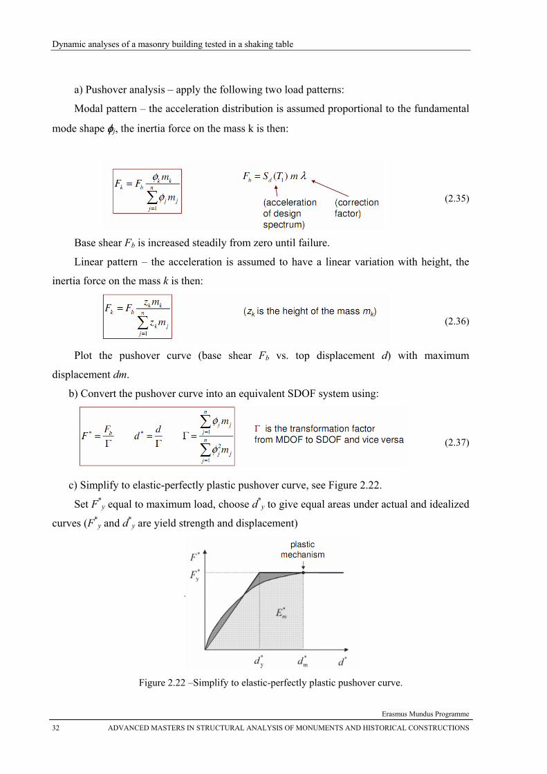
a) Pushover analysis – apply the following two load patterns:
Modal pattern – the acceleration distribution is assumed proportional to the fundamental
mode shape φj, the inertia force on the mass k is then:
(2.35)
Base shear Fb is increased steadily from zero until failure.
Linear pattern – the acceleration is assumed to have a linear variation with height, the
inertia force on the mass k is then:
(2.36)
Plot the pushover curve (base shear Fb vs. top displacement d) with maximum
displacement dm.
b) Convert the pushover curve into an equivalent SDOF system using:
(2.37)
c) Simplify to elastic-perfectly plastic pushover curve, see Figure 2.22.
Set F*y equal to maximum load, choose d*
y to give equal areas under actual and idealized
curves (F*y and d*
y are yield strength and displacement)
Figure 2.22 –Simplify to elastic-perfectly plastic pushover curve.
Chapter 2 – Basic Experimental and Numerical Methods in Earthquake Engineering
Erasmus Mundus Programme
ADVANCED MASTERS IN STRUCTURAL ANALYSIS OF MONUMENTS AND HISTORICAL CONSTRUCTIONS 33
d) Determine the period of idealized equivalent SDOF system
(2.38)
e) Calculate target displacement of SDOF system under design earthquake
(2.39)
(2.40)
(2.41)
f) Transform the target displacement back to that of the original MDOF system
(2.42)
Check that dt ≤ dm/1.5. Check member strengths and storey drifts are acceptable at the
value of dt.
2.5 Conclusion
In this chapter a state of the art of basic experimental and numerical methods in earthquake
engineering is presented. First, a brief introduction about the classic dynamic theory is carried
out. Then a review of the basic experimental and numerical methods is presented. Issues about
experimental methods addressed include in-situ vibration tests and laboratory tests. In the
vibration tests section, the basic techniques of the dynamic identification are also introduced,
followed by two typical cases of the in-situ vibration tests in historical structures; in the
laboratory tests section, the pseudo-dynamic tests and the shaking table tests are presented, with
the real cases addressed. After the experimental part, aspects related to numerical methods are
discussed, including time integration method and pushover method, which are the main means
to analyze the seismic behavior of the structures.
In this dissertation, the shaking table test results are used and time-integration methods are
adopted for the numerical analysis. In the following chapters, the detailed experimental
descriptions and analysis results will be presented.

Dynamic analyses of a masonry building tested in a shaking table
Erasmus Mundus Programme
34 ADVANCED MASTERS IN STRUCTURAL ANALYSIS OF MONUMENTS AND HISTORICAL CONSTRUCTIONS
Chapter 3 – Description of the Prototype and the Scaled Model in Shaking Table Tests
Erasmus Mundus Programme
ADVANCED MASTERS IN STRUCTURAL ANALYSIS OF MONUMENTS AND HISTORICAL CONSTRUCTIONS 35
CChhaapptteerr 33
DDeessccrriippttiioonn ooff tthhee PPrroottoottyyppee aanndd tthhee SSccaalleedd MMooddeell iinn SShhaakkiinngg TTaabbllee TTeessttss
Abstract In this chapter, a description of the prototype, the scaled mock-up and the numerical model is presented. First, a brief introduction on “Gaioleiro” prototype is provided, followed by the description of the shaking table tests previously carried out, including the scaled model, the equipments adopted and the testing procedures. Then the FEM model is introduced, detailing the calibration of the numerical model.
Dynamic analyses of a masonry building tested in a shaking table
Erasmus Mundus Programme
36 ADVANCED MASTERS IN STRUCTURAL ANALYSIS OF MONUMENTS AND HISTORICAL CONSTRUCTIONS
3.1 Introduction of the Prototype - Gaioleiro
As a typical case, the Gaioleiro building typology developed between the mid 19th century
and beginning of the 20th century, mainly in Lisbon and it still remains much in use nowadays.
These buildings characterize a transition period from the anti-seismic practices used in the
“pombalino” buildings originated after the earthquake of 1755 (Ramos and Lourenço, 2004),
and the modern reinforced concrete frame buildings.
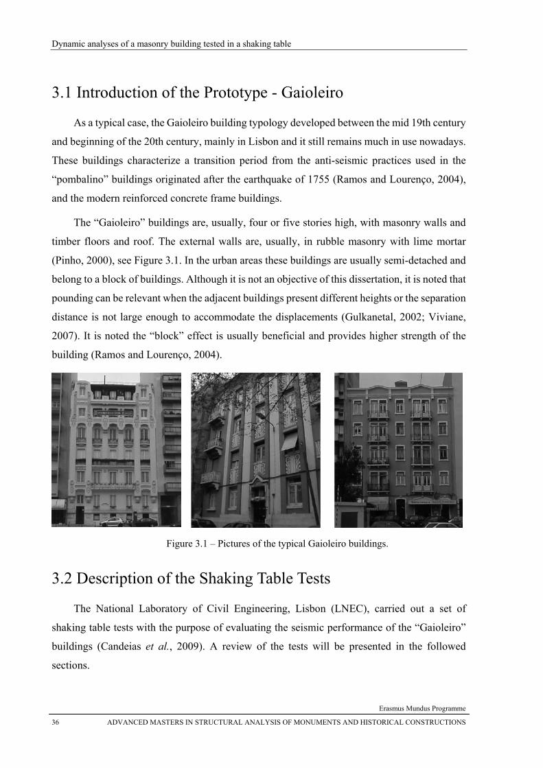
The “Gaioleiro” buildings are, usually, four or five stories high, with masonry walls and
timber floors and roof. The external walls are, usually, in rubble masonry with lime mortar
(Pinho, 2000), see Figure 3.1. In the urban areas these buildings are usually semi-detached and
belong to a block of buildings. Although it is not an objective of this dissertation, it is noted that
pounding can be relevant when the adjacent buildings present different heights or the separation
distance is not large enough to accommodate the displacements (Gulkanetal, 2002; Viviane,
2007). It is noted the “block” effect is usually beneficial and provides higher strength of the
building (Ramos and Lourenço, 2004).
Figure 3.1 – Pictures of the typical Gaioleiro buildings.
3.2 Description of the Shaking Table Tests
The National Laboratory of Civil Engineering, Lisbon (LNEC), carried out a set of
shaking table tests with the purpose of evaluating the seismic performance of the “Gaioleiro”
buildings (Candeias et al., 2009). A review of the tests will be presented in the followed
sections.
Chapter 3 – Description of the Prototype and the Scaled Model in Shaking Table Tests
Erasmus Mundus Programme
ADVANCED MASTERS IN STRUCTURAL ANALYSIS OF MONUMENTS AND HISTORICAL CONSTRUCTIONS 37
3.2.1 Introduction of the Mock-up
In order to study the seismic performance through experimental tests, a prototype of an
isolated building representative of the “Gaioleiro” buildings was defined. This is constituted by
four stories with an interstory height of 3.60 m and 9.45 m × 12.45 m in plan, two opposite
façades with a percentage of openings equal to 28.6% of the façade area, two opposite gable
walls (with no openings), timber floors, and a gable roof.
The mock-up was prepared to reproduce the geometrical, physical and dynamical
characteristics of the prototypes of buildings typologies. However, mock-ups are usually
simplified due to difficulties related to its reproduction in laboratory, namely the geometrical
properties of the prototype or individual structures and the size of the facilities. In fact, it is
difficult to fulfill the similitude laws using very small scales, such as the preparation of
masonry units and reinforcement elements.
Generally, in dynamic problems to be solved by experimental methods, the usual
similitude laws are the Cauchy Similitude and the Froude Similitude, which read, respectively,
E
2
ValueCauchy ρν= (3.1)
and
Lg
2
Value Froude ν= (3.2)
in which
ρ = specific mass v = velocity E = modulus of elasticity L = length g = acceleration of gravity
The Cauchy similitude is adequate for the phenomena in which the restoring forces are derived
from the stress-strain constitutive relation- ships. Alternatively, the Froude similitude is
adequate for phenomena in which the gravity forces are important as, for instance, the pendular
motion, or the flexural resistance of RC columns which depends on applied axial force
(Carvalho, 1998).
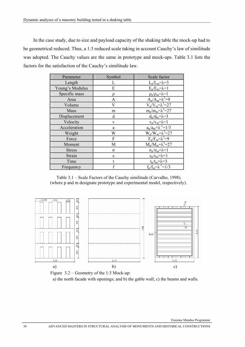
Dynamic analyses of a masonry building tested in a shaking table
Erasmus Mundus Programme
38 ADVANCED MASTERS IN STRUCTURAL ANALYSIS OF MONUMENTS AND HISTORICAL CONSTRUCTIONS
In the case study, due to size and payload capacity of the shaking table the mock-up had to
be geometrical reduced. Thus, a 1:3 reduced scale taking in account Cauchy’s law of similitude
was adopted. The Cauchy values are the same in prototype and mock-ups. Table 3.1 lists the
factors for the satisfaction of the Cauchy’s similitude law.
Parameter Symbol Scale factor Length L Lp/Lm=λ=3
Young’s Modulus E Ep/Em=λ=1 Specific mass ρ ρp/ρm=λ=1
Area A Ap/Am=λ2=9 Volume V Vp/Vm=λ3=27
Mass m mp/mm=λ3=27 Displacement d dp/dm=λ=3
Velocity v vp/vm=λ=1 Acceleration a ap/am=λ-1=1/3
Weight W Wp/Wm=λ3=27 Force F Fp/Fm=λ2=9
Moment M Mp/Mm=λ3=27 Stress σ σp/σm=λ=1 Strain ε εp/εm=λ=1 Time t tp/tm=λ=3
Frequency f fp/fm=λ-1=1/3
Table 3.1 – Scale Factors of the Cauchy similitude (Carvalho, 1998). (where p and m designate prototype and experimental model, respectively).
a) b) c)
Figure 3.2 – Geometry of the 1:3 Mock-up: a) the north facade with openings; and b) the gable wall; c) the beams and walls.
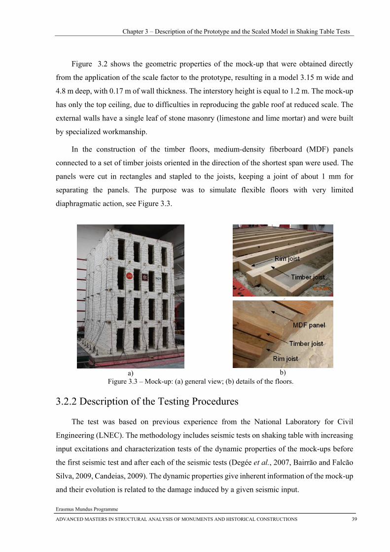
Chapter 3 – Description of the Prototype and the Scaled Model in Shaking Table Tests
Erasmus Mundus Programme
ADVANCED MASTERS IN STRUCTURAL ANALYSIS OF MONUMENTS AND HISTORICAL CONSTRUCTIONS 39
Figure 3.2 shows the geometric properties of the mock-up that were obtained directly
from the application of the scale factor to the prototype, resulting in a model 3.15 m wide and
4.8 m deep, with 0.17 m of wall thickness. The interstory height is equal to 1.2 m. The mock-up
has only the top ceiling, due to difficulties in reproducing the gable roof at reduced scale. The
external walls have a single leaf of stone masonry (limestone and lime mortar) and were built
by specialized workmanship.
In the construction of the timber floors, medium-density fiberboard (MDF) panels
connected to a set of timber joists oriented in the direction of the shortest span were used. The
panels were cut in rectangles and stapled to the joists, keeping a joint of about 1 mm for
separating the panels. The purpose was to simulate flexible floors with very limited
diaphragmatic action, see Figure 3.3.
a)
b)
Figure 3.3 – Mock-up: (a) general view; (b) details of the floors.
3.2.2 Description of the Testing Procedures
The test was based on previous experience from the National Laboratory for Civil
Engineering (LNEC). The methodology includes seismic tests on shaking table with increasing
input excitations and characterization tests of the dynamic properties of the mock-ups before
the first seismic test and after each of the seismic tests (Degée et al., 2007, Bairrão and Falcão
Silva, 2009, Candeias, 2009). The dynamic properties give inherent information of the mock-up
and their evolution is related to the damage induced by a given seismic input.
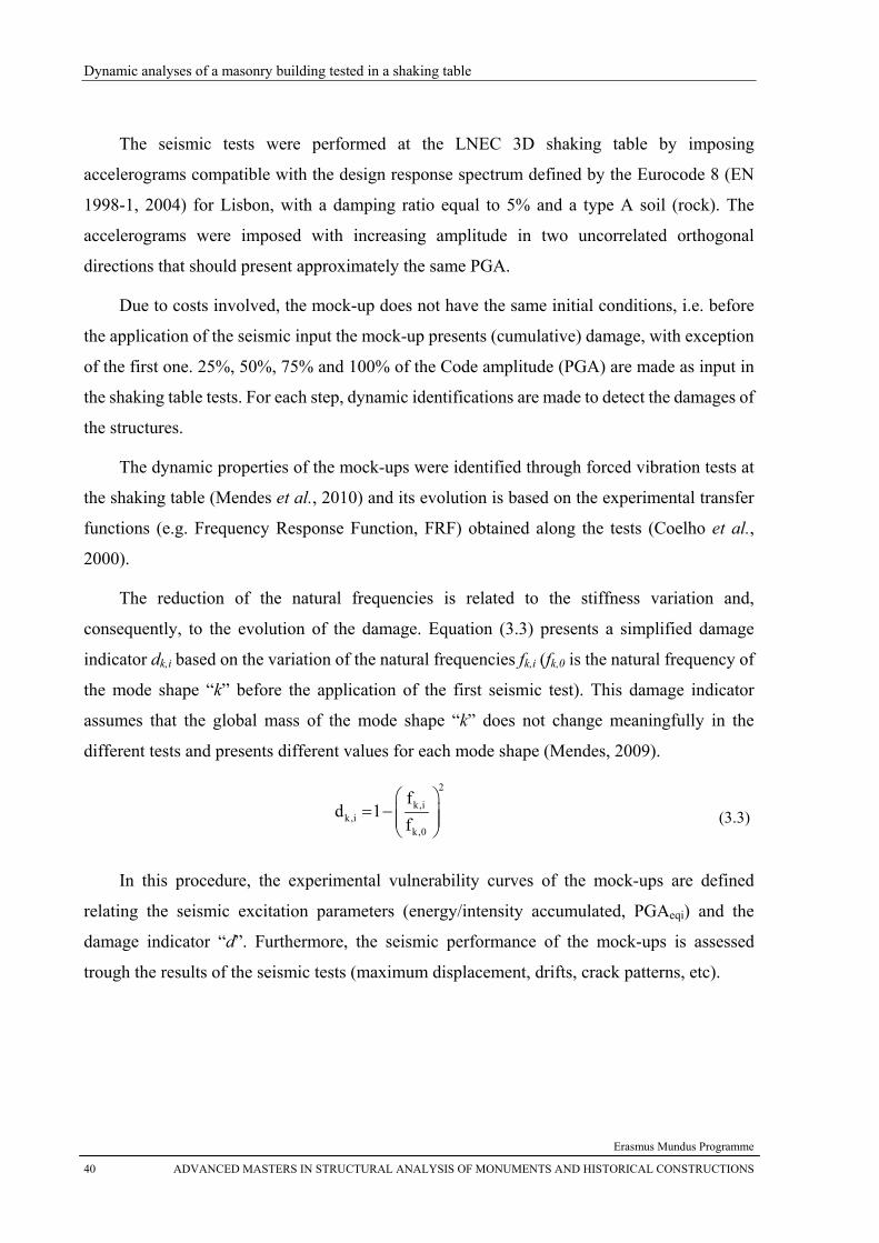
Dynamic analyses of a masonry building tested in a shaking table
Erasmus Mundus Programme
40 ADVANCED MASTERS IN STRUCTURAL ANALYSIS OF MONUMENTS AND HISTORICAL CONSTRUCTIONS
The seismic tests were performed at the LNEC 3D shaking table by imposing
accelerograms compatible with the design response spectrum defined by the Eurocode 8 (EN
1998-1, 2004) for Lisbon, with a damping ratio equal to 5% and a type A soil (rock). The
accelerograms were imposed with increasing amplitude in two uncorrelated orthogonal
directions that should present approximately the same PGA.
Due to costs involved, the mock-up does not have the same initial conditions, i.e. before
the application of the seismic input the mock-up presents (cumulative) damage, with exception
of the first one. 25%, 50%, 75% and 100% of the Code amplitude (PGA) are made as input in
the shaking table tests. For each step, dynamic identifications are made to detect the damages of
the structures.
The dynamic properties of the mock-ups were identified through forced vibration tests at
the shaking table (Mendes et al., 2010) and its evolution is based on the experimental transfer
functions (e.g. Frequency Response Function, FRF) obtained along the tests (Coelho et al.,
2000).
The reduction of the natural frequencies is related to the stiffness variation and,
consequently, to the evolution of the damage. Equation (3.3) presents a simplified damage
indicator dk,i based on the variation of the natural frequencies fk,i (fk,0 is the natural frequency of
the mode shape “k” before the application of the first seismic test). This damage indicator
assumes that the global mass of the mode shape “k” does not change meaningfully in the
different tests and presents different values for each mode shape (Mendes, 2009).
2
k,ik,i
k,0
fd 1
f⎛ ⎞
= − ⎜ ⎟⎜ ⎟⎝ ⎠
(3.3)
In this procedure, the experimental vulnerability curves of the mock-ups are defined
relating the seismic excitation parameters (energy/intensity accumulated, PGAeqi) and the
damage indicator “d”. Furthermore, the seismic performance of the mock-ups is assessed
trough the results of the seismic tests (maximum displacement, drifts, crack patterns, etc).
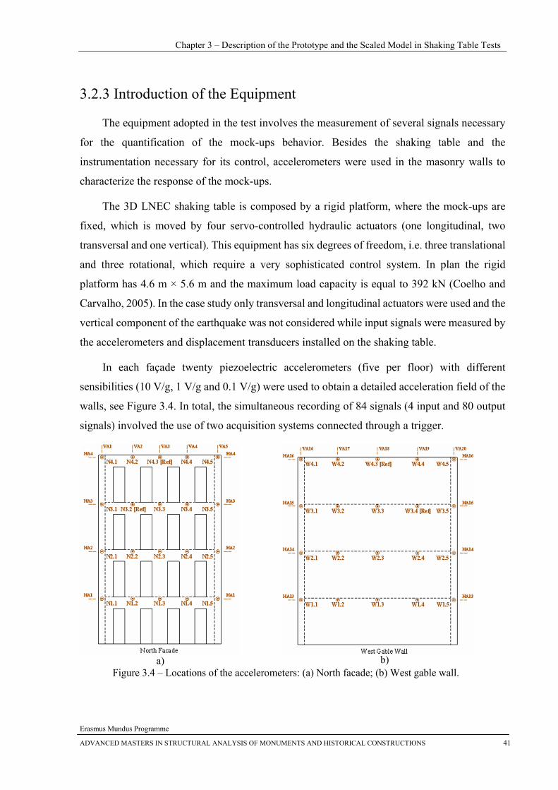
Chapter 3 – Description of the Prototype and the Scaled Model in Shaking Table Tests
Erasmus Mundus Programme
ADVANCED MASTERS IN STRUCTURAL ANALYSIS OF MONUMENTS AND HISTORICAL CONSTRUCTIONS 41
3.2.3 Introduction of the Equipment
The equipment adopted in the test involves the measurement of several signals necessary
for the quantification of the mock-ups behavior. Besides the shaking table and the
instrumentation necessary for its control, accelerometers were used in the masonry walls to
characterize the response of the mock-ups.
The 3D LNEC shaking table is composed by a rigid platform, where the mock-ups are
fixed, which is moved by four servo-controlled hydraulic actuators (one longitudinal, two
transversal and one vertical). This equipment has six degrees of freedom, i.e. three translational
and three rotational, which require a very sophisticated control system. In plan the rigid
platform has 4.6 m × 5.6 m and the maximum load capacity is equal to 392 kN (Coelho and
Carvalho, 2005). In the case study only transversal and longitudinal actuators were used and the
vertical component of the earthquake was not considered while input signals were measured by
the accelerometers and displacement transducers installed on the shaking table.
In each façade twenty piezoelectric accelerometers (five per floor) with different
sensibilities (10 V/g, 1 V/g and 0.1 V/g) were used to obtain a detailed acceleration field of the
walls, see Figure 3.4. In total, the simultaneous recording of 84 signals (4 input and 80 output
signals) involved the use of two acquisition systems connected through a trigger.
a)
b) Figure 3.4 – Locations of the accelerometers: (a) North facade; (b) West gable wall.
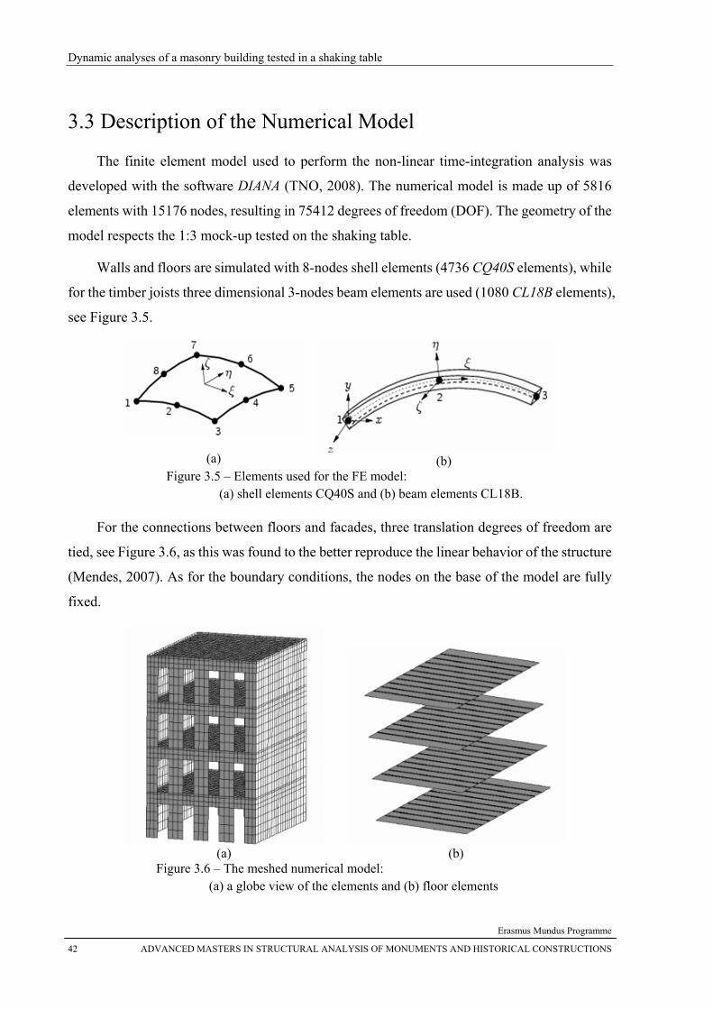
Dynamic analyses of a masonry building tested in a shaking table
Erasmus Mundus Programme
42 ADVANCED MASTERS IN STRUCTURAL ANALYSIS OF MONUMENTS AND HISTORICAL CONSTRUCTIONS
3.3 Description of the Numerical Model
The finite element model used to perform the non-linear time-integration analysis was
developed with the software DIANA (TNO, 2008). The numerical model is made up of 5816
elements with 15176 nodes, resulting in 75412 degrees of freedom (DOF). The geometry of the
model respects the 1:3 mock-up tested on the shaking table.
Walls and floors are simulated with 8-nodes shell elements (4736 CQ40S elements), while
for the timber joists three dimensional 3-nodes beam elements are used (1080 CL18B elements),
see Figure 3.5.
(a)
(b)
Figure 3.5 – Elements used for the FE model: (a) shell elements CQ40S and (b) beam elements CL18B.
For the connections between floors and facades, three translation degrees of freedom are
tied, see Figure 3.6, as this was found to the better reproduce the linear behavior of the structure
(Mendes, 2007). As for the boundary conditions, the nodes on the base of the model are fully
fixed.
(a)
(b)
Figure 3.6 – The meshed numerical model: (a) a globe view of the elements and (b) floor elements
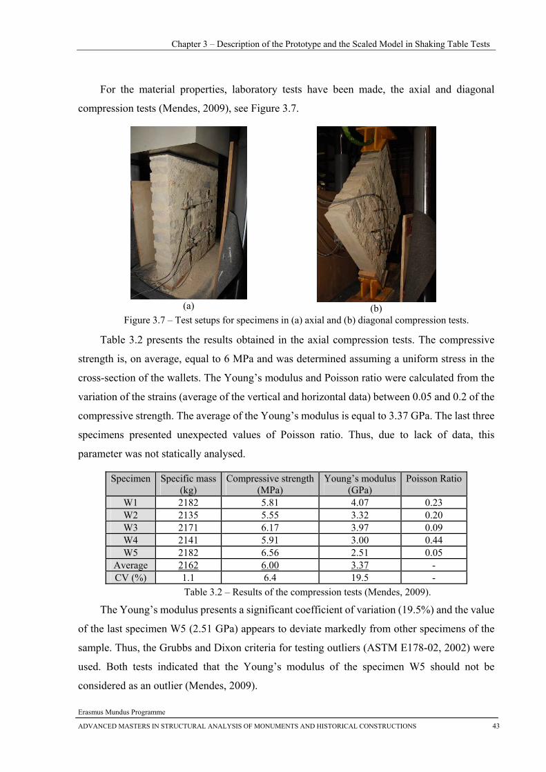
Chapter 3 – Description of the Prototype and the Scaled Model in Shaking Table Tests
Erasmus Mundus Programme
ADVANCED MASTERS IN STRUCTURAL ANALYSIS OF MONUMENTS AND HISTORICAL CONSTRUCTIONS 43
For the material properties, laboratory tests have been made, the axial and diagonal
compression tests (Mendes, 2009), see Figure 3.7.
(a)
(b)
Figure 3.7 – Test setups for specimens in (a) axial and (b) diagonal compression tests.
Table 3.2 presents the results obtained in the axial compression tests. The compressive
strength is, on average, equal to 6 MPa and was determined assuming a uniform stress in the
cross-section of the wallets. The Young’s modulus and Poisson ratio were calculated from the
variation of the strains (average of the vertical and horizontal data) between 0.05 and 0.2 of the
compressive strength. The average of the Young’s modulus is equal to 3.37 GPa. The last three
specimens presented unexpected values of Poisson ratio. Thus, due to lack of data, this
parameter was not statically analysed.
Specimen Specific mass (kg)
Compressive strength(MPa)
Young’s modulus (GPa)
Poisson Ratio
W1 2182 5.81 4.07 0.23 W2 2135 5.55 3.32 0.20 W3 2171 6.17 3.97 0.09 W4 2141 5.91 3.00 0.44 W5 2182 6.56 2.51 0.05
Average 2162 6.00 3.37 - CV (%) 1.1 6.4 19.5 -
Table 3.2 – Results of the compression tests (Mendes, 2009).
The Young’s modulus presents a significant coefficient of variation (19.5%) and the value
of the last specimen W5 (2.51 GPa) appears to deviate markedly from other specimens of the
sample. Thus, the Grubbs and Dixon criteria for testing outliers (ASTM E178-02, 2002) were
used. Both tests indicated that the Young’s modulus of the specimen W5 should not be
considered as an outlier (Mendes, 2009).
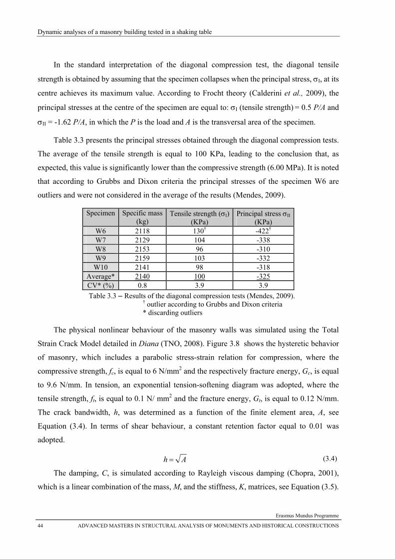
Dynamic analyses of a masonry building tested in a shaking table
Erasmus Mundus Programme
44 ADVANCED MASTERS IN STRUCTURAL ANALYSIS OF MONUMENTS AND HISTORICAL CONSTRUCTIONS
In the standard interpretation of the diagonal compression test, the diagonal tensile
strength is obtained by assuming that the specimen collapses when the principal stress, σI, at its
centre achieves its maximum value. According to Frocht theory (Calderini et al., 2009), the
principal stresses at the centre of the specimen are equal to: σI (tensile strength) = 0.5 P/A and
σII = -1.62 P/A, in which the P is the load and A is the transversal area of the specimen.
Table 3.3 presents the principal stresses obtained through the diagonal compression tests.
The average of the tensile strength is equal to 100 KPa, leading to the conclusion that, as
expected, this value is significantly lower than the compressive strength (6.00 MPa). It is noted
that according to Grubbs and Dixon criteria the principal stresses of the specimen W6 are
outliers and were not considered in the average of the results (Mendes, 2009).
Specimen Specific mass (kg)
Tensile strength (σI)(KPa)
Principal stress σII (KPa)
W6 2118 130† -422† W7 2129 104 -338 W8 2153 96 -310 W9 2159 103 -332
W10 2141 98 -318 Average* 2140 100 -325 CV* (%) 0.8 3.9 3.9 Table 3.3 – Results of the diagonal compression tests (Mendes, 2009).
† outlier according to Grubbs and Dixon criteria * discarding outliers
The physical nonlinear behaviour of the masonry walls was simulated using the Total
Strain Crack Model detailed in Diana (TNO, 2008). Figure 3.8 shows the hysteretic behavior
of masonry, which includes a parabolic stress-strain relation for compression, where the
compressive strength, fc, is equal to 6 N/mm2 and the respectively fracture energy, Gc, is equal
to 9.6 N/mm. In tension, an exponential tension-softening diagram was adopted, where the
tensile strength, ft, is equal to 0.1 N/ mm2 and the fracture energy, Gt, is equal to 0.12 N/mm.
The crack bandwidth, h, was determined as a function of the finite element area, A, see
Equation (3.4). In terms of shear behaviour, a constant retention factor equal to 0.01 was
adopted.
Ah = (3.4)
The damping, C, is simulated according to Rayleigh viscous damping (Chopra, 2001),
which is a linear combination of the mass, M, and the stiffness, K, matrices, see Equation (3.5).
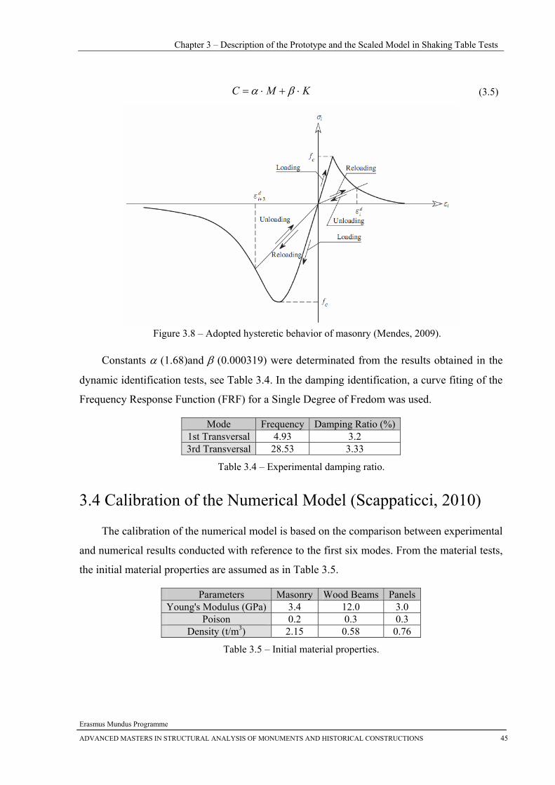
Chapter 3 – Description of the Prototype and the Scaled Model in Shaking Table Tests
Erasmus Mundus Programme
ADVANCED MASTERS IN STRUCTURAL ANALYSIS OF MONUMENTS AND HISTORICAL CONSTRUCTIONS 45
KMC ⋅+⋅= βα (3.5)
Figure 3.8 – Adopted hysteretic behavior of masonry (Mendes, 2009).
Constants α (1.68)and β (0.000319) were determinated from the results obtained in the
dynamic identification tests, see Table 3.4. In the damping identification, a curve fiting of the
Frequency Response Function (FRF) for a Single Degree of Fredom was used.
Mode Frequency Damping Ratio (%) 1st Transversal 4.93 3.2 3rd Transversal 28.53 3.33
Table 3.4 – Experimental damping ratio.
3.4 Calibration of the Numerical Model (Scappaticci, 2010)
The calibration of the numerical model is based on the comparison between experimental
and numerical results conducted with reference to the first six modes. From the material tests,
the initial material properties are assumed as in Table 3.5.
Parameters Masonry Wood Beams Panels Young's Modulus (GPa) 3.4 12.0 3.0
Poison 0.2 0.3 0.3 Density (t/m3) 2.15 0.58 0.76
Table 3.5 – Initial material properties.
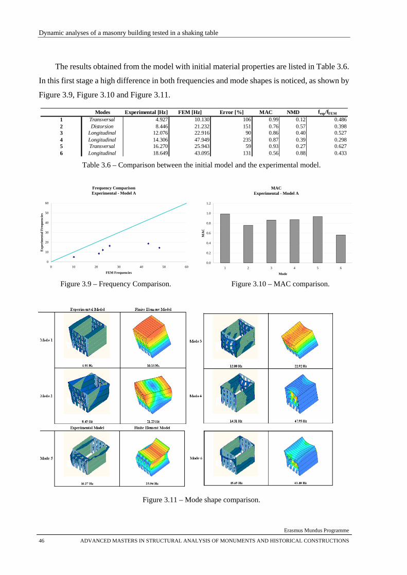
Dynamic analyses of a masonry building tested in a shaking table
Erasmus Mundus Programme
46 ADVANCED MASTERS IN STRUCTURAL ANALYSIS OF MONUMENTS AND HISTORICAL CONSTRUCTIONS
The results obtained from the model with initial material properties are listed in Table 3.6.
In this first stage a high difference in both frequencies and mode shapes is noticed, as shown by
Figure 3.9, Figure 3.10 and Figure 3.11.
Modes Experimental [Hz] FEM [Hz] Error [%] MAC NMD fexp/fFEM
1 Transversal 4.927 10.130 106 0.99 0.12 0.4862 Distorsion 8.446 21.232 151 0.76 0.57 0.3983 Longitudinal 12.076 22.916 90 0.86 0.40 0.5274 Longitudinal 14.306 47.949 235 0.87 0.39 0.2985 Transversal 16.270 25.943 59 0.93 0.27 0.6276 Longitudinal 18.649 43.095 131 0.56 0.88 0.433
Table 3.6 – Comparison between the initial model and the experimental model.
Frequency ComparisonExperimental - Model A
0
10
20
30
40
50
60
0 10 20 30 40 50 60
FEM Frequencies
Exp
erim
enta
l Fre
quen
cies
MACExperimental - Model A
0.0
0.2
0.4
0.6
0.8
1.0
1.2
1 2 3 4 5 6
Mode
MA
C
Figure 3.9 – Frequency Comparison. Figure 3.10 – MAC comparison.
Figure 3.11 – Mode shape comparison.
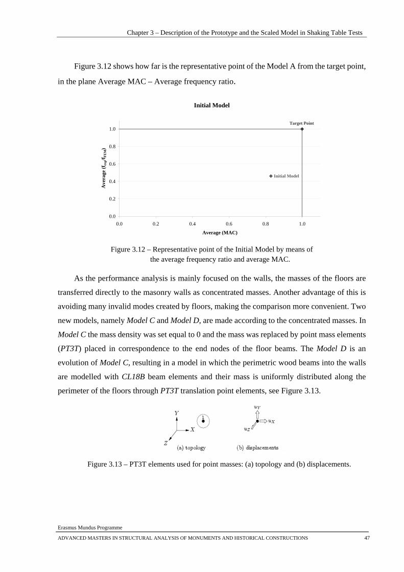
Chapter 3 – Description of the Prototype and the Scaled Model in Shaking Table Tests
Erasmus Mundus Programme
ADVANCED MASTERS IN STRUCTURAL ANALYSIS OF MONUMENTS AND HISTORICAL CONSTRUCTIONS 47
Figure 3.12 shows how far is the representative point of the Model A from the target point,
in the plane Average MAC – Average frequency ratio.
Initial Model
Initial Model
Target Point
0.0
0.2
0.4
0.6
0.8
1.0
0.0 0.2 0.4 0.6 0.8 1.0
Average (MAC)
Ave
rage
(fex
p/fFE
M)
Figure 3.12 – Representative point of the Initial Model by means of
the average frequency ratio and average MAC.
As the performance analysis is mainly focused on the walls, the masses of the floors are
transferred directly to the masonry walls as concentrated masses. Another advantage of this is
avoiding many invalid modes created by floors, making the comparison more convenient. Two
new models, namely Model C and Model D, are made according to the concentrated masses. In
Model C the mass density was set equal to 0 and the mass was replaced by point mass elements
(PT3T) placed in correspondence to the end nodes of the floor beams. The Model D is an
evolution of Model C, resulting in a model in which the perimetric wood beams into the walls
are modelled with CL18B beam elements and their mass is uniformly distributed along the
perimeter of the floors through PT3T translation point elements, see Figure 3.13.
Figure 3.13 – PT3T elements used for point masses: (a) topology and (b) displacements.
Dynamic analyses of a masonry building tested in a shaking table
Erasmus Mundus Programme
48 ADVANCED MASTERS IN STRUCTURAL ANALYSIS OF MONUMENTS AND HISTORICAL CONSTRUCTIONS
Table 3.7 – Frequencies of the two new models.
Table 3.7 lists the frequencies of Model C and Model D, and their difference is rather small.
However the difference between the experimental and numerical model remains high,
especially in frequencies. Assuming that the geometric definition of the model is correct, the
source of difference can be attributed to an inappropriate estimation of the elastic modulus of
masonry.
From the orthogonal test shown in Table 3.8, the sensitivity of the results to the Young’s
modulus of the floor elements is obtained. It is shown that the Young’s modulus of the wood
beams has little influence on the variability of frequencies, while decreasing the Young’s
modulus of panels can produce a significant increase in the ratio fexp/fFEM, see Table
3.9.Subsequently, sensitivities of other components will also be obtained.
MODEL FACADES GABLE WALLS WOOD BEAMS PANELS1 3.4 3.4 10.0 2.02 3.4 3.4 12.0 2.03 3.4 3.4 14.0 2.04 3.4 3.4 10.0 3.05 3.4 3.4 12.0 3.06 3.4 3.4 14.0 3.07 3.4 3.4 10.0 4.08 3.4 3.4 12.0 4.09 3.4 3.4 14.0 4.0
Table 3.8 – Material Properties of the models analysed in the first Step of the Sensitivity Analysis..
MODE MODEL 1 MODEL 2 MODEL 3 MODEL 4 MODEL 5 MODEL 6 MODEL 7 MODEL 8 MODEL 91 10.03 10.05 10.06 10.16 10.17 10.18 10.23 10.24 10.252 20.11 20.13 20.14 21.18 21.20 21.21 21.78 21.80 21.823 22.66 22.67 22.68 23.05 23.06 23.07 23.25 23.26 23.274 41.75 41.90 42.01 48.39 48.59 48.75 53.62 53.89 54.095 24.38 24.41 24.43 25.93 25.96 25.99 26.94 26.97 27.016 39.51 39.58 39.65 44.19 44.26 44.33 47.71 47.78 47.84
FREQUENCIES
Table 3.9 – Frequency Comparison in the first Step of the Sensitivity Analysis.
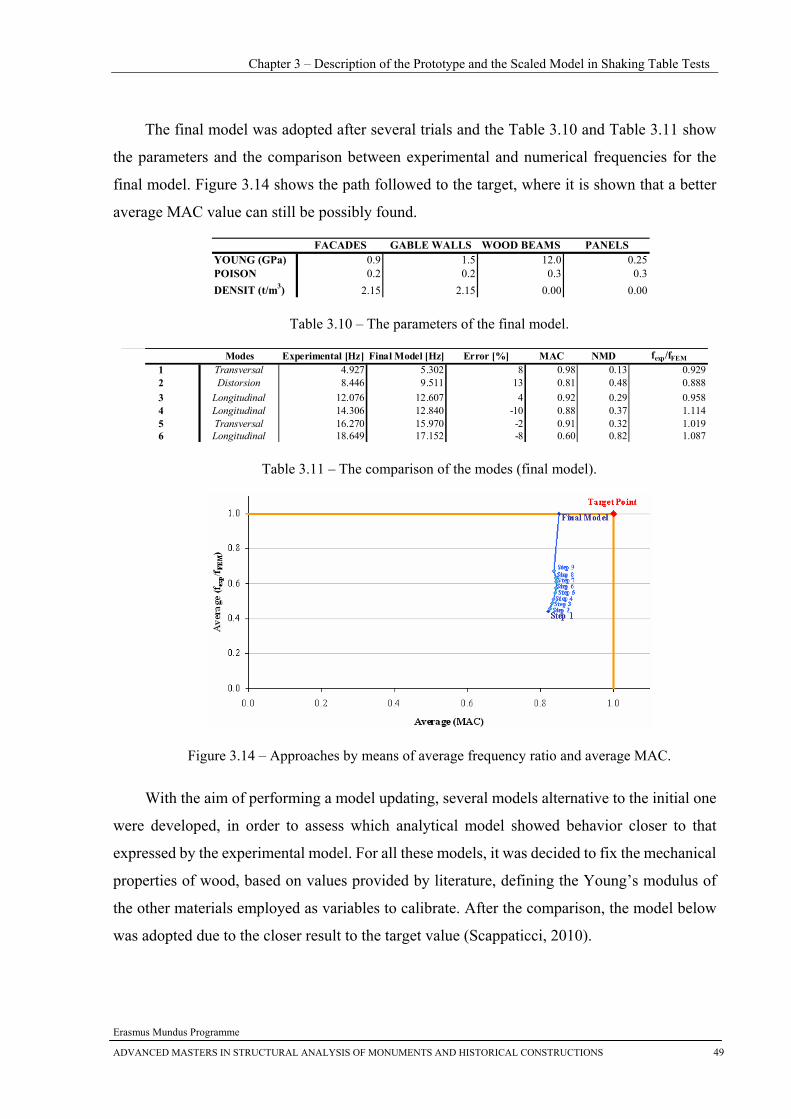
Chapter 3 – Description of the Prototype and the Scaled Model in Shaking Table Tests
Erasmus Mundus Programme
ADVANCED MASTERS IN STRUCTURAL ANALYSIS OF MONUMENTS AND HISTORICAL CONSTRUCTIONS 49
The final model was adopted after several trials and the Table 3.10 and Table 3.11 show
the parameters and the comparison between experimental and numerical frequencies for the
final model. Figure 3.14 shows the path followed to the target, where it is shown that a better
average MAC value can still be possibly found.
FACADES GABLE WALLS WOOD BEAMS PANELSYOUNG (GPa) 0.9 1.5 12.0 0.25POISON 0.2 0.2 0.3 0.3DENSIT (t/m3) 2.15 2.15 0.00 0.00
Table 3.10 – The parameters of the final model.
Modes Experimental [Hz] Final Model [Hz] Error [%] MAC NMD fexp/fFEM
1 Transversal 4.927 5.302 8 0.98 0.13 0.9292 Distorsion 8.446 9.511 13 0.81 0.48 0.8883 Longitudinal 12.076 12.607 4 0.92 0.29 0.9584 Longitudinal 14.306 12.840 -10 0.88 0.37 1.1145 Transversal 16.270 15.970 -2 0.91 0.32 1.0196 Longitudinal 18.649 17.152 -8 0.60 0.82 1.087
Table 3.11 – The comparison of the modes (final model).
Figure 3.14 – Approaches by means of average frequency ratio and average MAC.
With the aim of performing a model updating, several models alternative to the initial one
were developed, in order to assess which analytical model showed behavior closer to that
expressed by the experimental model. For all these models, it was decided to fix the mechanical
properties of wood, based on values provided by literature, defining the Young’s modulus of
the other materials employed as variables to calibrate. After the comparison, the model below
was adopted due to the closer result to the target value (Scappaticci, 2010).
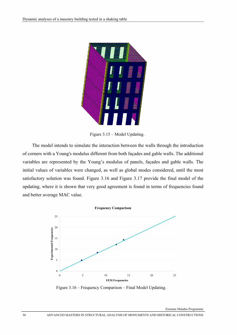
Dynamic analyses of a masonry building tested in a shaking table
Erasmus Mundus Programme
50 ADVANCED MASTERS IN STRUCTURAL ANALYSIS OF MONUMENTS AND HISTORICAL CONSTRUCTIONS
Figure 3.15 – Model Updating.
The model intends to simulate the interaction between the walls through the introduction
of corners with a Young's modulus different from both façades and gable walls. The additional
variables are represented by the Young’s modulus of panels, façades and gable walls. The
initial values of variables were changed, as well as global modes considered, until the most
satisfactory solution was found. Figure 3.16 and Figure 3.17 provide the final model of the
updating, where it is shown that very good agreement is found in terms of frequencies found
and better average MAC value.
Frequency Comparison
0
5
10
15
20
25
0 5 10 15 20 25
FEM Frequencies
Exp
erim
enta
l Fre
quen
cies
Figure 3.16 – Frequency Comparison – Final Model Updating.
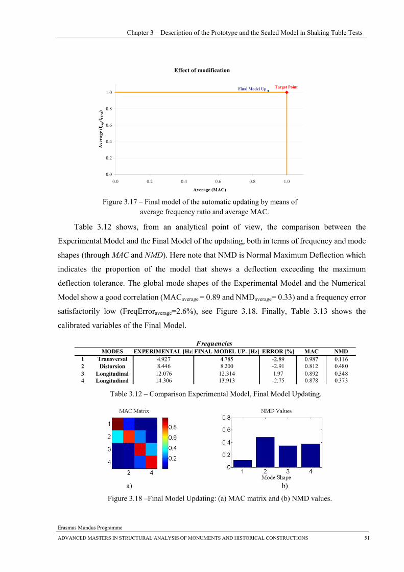
Chapter 3 – Description of the Prototype and the Scaled Model in Shaking Table Tests
Erasmus Mundus Programme
ADVANCED MASTERS IN STRUCTURAL ANALYSIS OF MONUMENTS AND HISTORICAL CONSTRUCTIONS 51
Effect of modification
Target PointFinal Model Up
0.0
0.2
0.4
0.6
0.8
1.0
0.0 0.2 0.4 0.6 0.8 1.0
Average (MAC)
Ave
rage
(fex
p/fFE
M)
Figure 3.17 – Final model of the automatic updating by means of
average frequency ratio and average MAC.
Table 3.12 shows, from an analytical point of view, the comparison between the
Experimental Model and the Final Model of the updating, both in terms of frequency and mode
shapes (through MAC and NMD). Here note that NMD is Normal Maximum Deflection which
indicates the proportion of the model that shows a deflection exceeding the maximum
deflection tolerance. The global mode shapes of the Experimental Model and the Numerical
Model show a good correlation (MACaverage = 0.89 and NMDaverage= 0.33) and a frequency error
satisfactorily low (FreqErroraverage=2.6%), see Figure 3.18. Finally, Table 3.13 shows the
calibrated variables of the Final Model.
MODES EXPERIMENTAL [Hz]FINAL MODEL UP. [Hz] ERROR [%] MAC NMD1 Transversal 4.927 4.785 -2.89 0.987 0.1162 Distorsion 8.446 8.200 -2.91 0.812 0.4803 Longitudinal 12.076 12.314 1.97 0.892 0.3484 Longitudinal 14.306 13.913 -2.75 0.878 0.373
Frequencies
Table 3.12 – Comparison Experimental Model, Final Model Updating.
a) b)
Figure 3.18 –Final Model Updating: (a) MAC matrix and (b) NMD values.
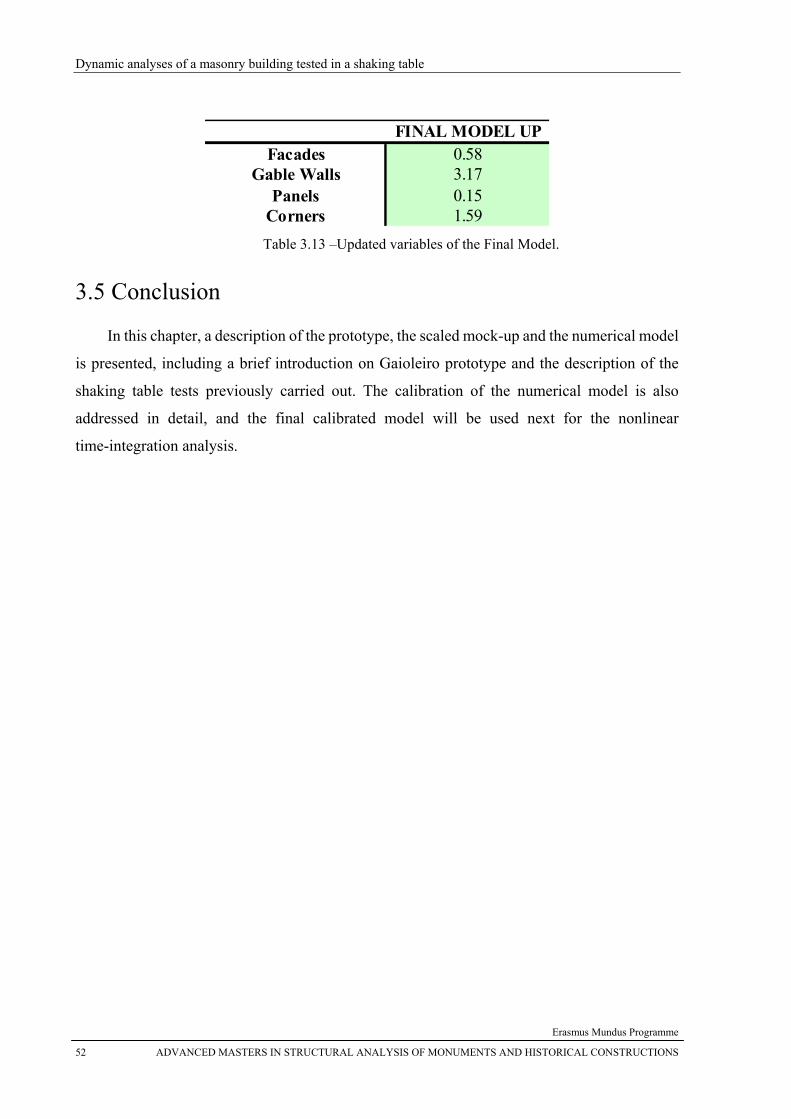
Dynamic analyses of a masonry building tested in a shaking table
Erasmus Mundus Programme
52 ADVANCED MASTERS IN STRUCTURAL ANALYSIS OF MONUMENTS AND HISTORICAL CONSTRUCTIONS
FINAL MODEL UPFacades 0.58
Gable Walls 3.17Panels 0.15
Corners 1.59 Table 3.13 –Updated variables of the Final Model.
3.5 Conclusion
In this chapter, a description of the prototype, the scaled mock-up and the numerical model
is presented, including a brief introduction on Gaioleiro prototype and the description of the
shaking table tests previously carried out. The calibration of the numerical model is also
addressed in detail, and the final calibrated model will be used next for the nonlinear
time-integration analysis.
Chapter 4 – Dynamic Analysis of the Scaled Model
Erasmus Mundus Programme
ADVANCED MASTERS IN STRUCTURAL ANALYSIS OF MONUMENTS AND HISTORICAL CONSTRUCTIONS 53
CChhaapptteerr 44
DDyynnaammiicc AAnnaallyyssiiss ooff tthhee SSccaalleedd MMooddeell
Abstract This chapter presents an analysis of the experimental and numerical results of the scaled model. First, for the purpose of optimization, five different numerical models are used for time- integration analysis, and then compared with the experimental data for 25% of the Peak Ground Acceleration (PGA). Then, the selected model is used for the 100% of the PGA. Aspects considered in the comparison include: a) the accelerations and displacements of 80 typical points in four façades; b) piers on North/South facades; c) the maximum strain on each facade and the crack patterns; d) the damage factor after the 25% and 100% of the PGA.
Dynamic analyses of a masonry building tested in a shaking table
Erasmus Mundus Programme
54 ADVANCED MASTERS IN STRUCTURAL ANALYSIS OF MONUMENTS AND HISTORICAL CONSTRUCTIONS
4.1 Description of the Nonlinear Time-Integration Analysis
The nonlinear time-integration analysis for masonry structures is more complicated than
steel-concrete or steel structures because of the low tensile strength of the material. In the case
of steel-concrete or steel structures the plastic hinges obviously occur in the overstressed parts,
whereas, in masonry, distributed cracks appear. The use of softening tends to lead to
convergence problems even for static problems, due to the fact that an ill-conditioned problem
appears, and matrices are usually rebuilt in every step, making the analyses rather
time-consuming. The quasi-brittle behaviour of the material in tension also introduces
numerical noise, due to the fast transition from linear elastic behaviour to a fully cracked state
involving almost zero stiffness. The quasi-instantaneous changes in the displacement field tend
to originate the propagation of high frequency spurious vibrations (Cervera et al., 1995).
Therefore, it is important to adopt the Hilbert-Hughes-Taylor time integration method (DIANA,
2005) (also called the α-method), which was used here with α equal to –0.1. With this method it
is possible to introduce numerical dissipation without degrading the accuracy (Mendes and
Lourenço, 2010). The Hilbert-Hughes-Taylor method uses the same finite difference equations
as the Newmark method with:
(4.1)
and
(4.2)
For α = 0 the method reduces to the Newmark method (see Chapter 2). For α between -1/3
and 1/2 the scheme is second-order accurate and unconditionally stable. Decreasing α means
increasing the numerical damping, and the adopted damping is low for low-frequency modes
and high for the high-frequencies modes.
The seismic tests were performed at the LNEC 3D shaking table by imposing
accelerograms compatible with the design response spectrum defined by the Eurocode 8 (EN
1998-1, 2004) for Lisbon, with a damping ratio equal to 5% and a type A soil (rock). Figure 4.1
shows the response curve of the input and the Eurocode 8. Using the 1:3 reduced scale, the
accelerograms have a total duration of 12s, and a PGA equal to 0.475g = 4.66 m/s2. The
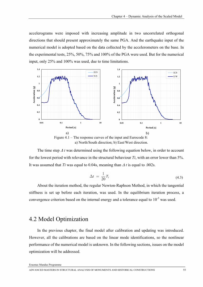
Chapter 4 – Dynamic Analysis of the Scaled Model
Erasmus Mundus Programme
ADVANCED MASTERS IN STRUCTURAL ANALYSIS OF MONUMENTS AND HISTORICAL CONSTRUCTIONS 55
accelerograms were imposed with increasing amplitude in two uncorrelated orthogonal
directions that should present approximately the same PGA. And the earthquake input of the
numerical model is adopted based on the data collected by the accelerometers on the base. In
the experimental tests, 25%, 50%, 75% and 100% of the PGA were used. But for the numerical
input, only 25% and 100% was used, due to time limitations.
0
0.2
0.4
0.6
0.8
1
1.2
1.4
0.01 0.1 1 10
Period [s]
Acc
eler
atio
n [g
]
EC8N/S
a)
0
0.2
0.4
0.6
0.8
1
1.2
1.4
0.01 0.1 1 10
Period [s]
Acc
eler
atio
n [g
]
EC8E/W
b)
Figure 4.1 – The response curves of the input and Eurocode 8: a) North/South direction; b) East/West direction.
The time step Δ t was determined using the following equation below, in order to account
for the lowest period with relevance in the structural behaviour Ti, with an error lower than 5%.
It was assumed that Ti was equal to 0.04s, meaning than Δ t is equal to .002s.
(4.3)
About the iteration method, the regular Newton-Raphson Method, in which the tangential
stiffness is set up before each iteration, was used. In the equilibrium iteration process, a
convergence criterion based on the internal energy and a tolerance equal to 10-3 was used.
4.2 Model Optimization
In the previous chapter, the final model after calibration and updating was introduced.
However, all the calibrations are based on the linear mode identifications, so the nonlinear
performance of the numerical model is unknown. In the following sections, issues on the model
optimization will be addressed.
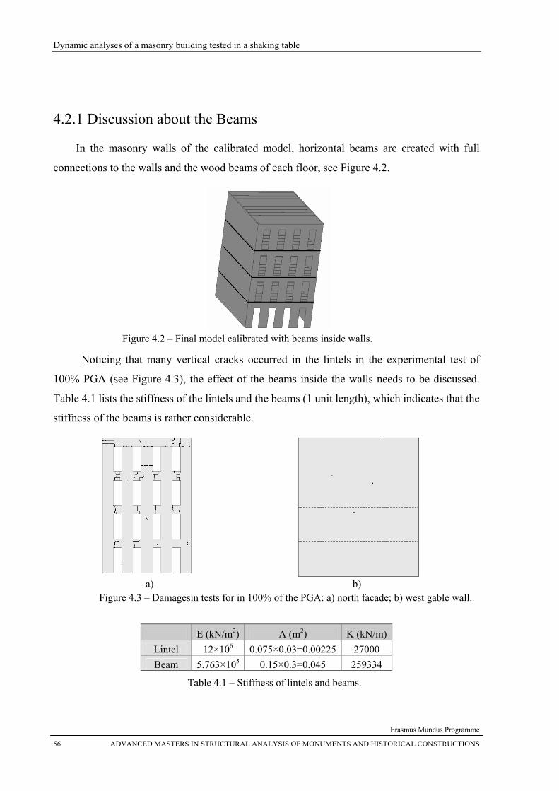
Dynamic analyses of a masonry building tested in a shaking table
Erasmus Mundus Programme
56 ADVANCED MASTERS IN STRUCTURAL ANALYSIS OF MONUMENTS AND HISTORICAL CONSTRUCTIONS
4.2.1 Discussion about the Beams
In the masonry walls of the calibrated model, horizontal beams are created with full
connections to the walls and the wood beams of each floor, see Figure 4.2.
Figure 4.2 – Final model calibrated with beams inside walls.
Noticing that many vertical cracks occurred in the lintels in the experimental test of
100% PGA (see Figure 4.3), the effect of the beams inside the walls needs to be discussed.
Table 4.1 lists the stiffness of the lintels and the beams (1 unit length), which indicates that the
stiffness of the beams is rather considerable.
a) b)
Figure 4.3 – Damagesin tests for in 100% of the PGA: a) north facade; b) west gable wall.
E (kN/m2) A (m2) K (kN/m)Lintel 12×106 0.075×0.03=0.00225 27000 Beam 5.763×10⁵ 0.15×0.3=0.045 259334
Table 4.1 – Stiffness of lintels and beams.
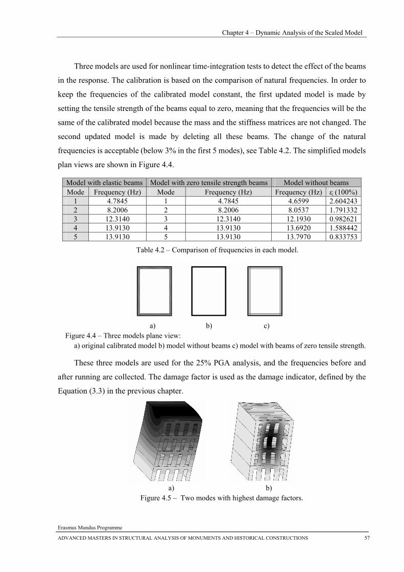
Chapter 4 – Dynamic Analysis of the Scaled Model
Erasmus Mundus Programme
ADVANCED MASTERS IN STRUCTURAL ANALYSIS OF MONUMENTS AND HISTORICAL CONSTRUCTIONS 57
Three models are used for nonlinear time-integration tests to detect the effect of the beams
in the response. The calibration is based on the comparison of natural frequencies. In order to
keep the frequencies of the calibrated model constant, the first updated model is made by
setting the tensile strength of the beams equal to zero, meaning that the frequencies will be the
same of the calibrated model because the mass and the stiffness matrices are not changed. The
second updated model is made by deleting all these beams. The change of the natural
frequencies is acceptable (below 3% in the first 5 modes), see Table 4.2. The simplified models
plan views are shown in Figure 4.4.
Model with elastic beams Model with zero tensile strength beams Model without beams Mode Frequency (Hz) Mode Frequency (Hz) Frequency (Hz) ε (100%)
1 4.7845 1 4.7845 4.6599 2.604243 2 8.2006 2 8.2006 8.0537 1.791332 3 12.3140 3 12.3140 12.1930 0.982621 4 13.9130 4 13.9130 13.6920 1.588442 5 13.9130 5 13.9130 13.7970 0.833753
Table 4.2 – Comparison of frequencies in each model.
a) b) c)
Figure 4.4 – Three models plane view: a) original calibrated model b) model without beams c) model with beams of zero tensile strength.
These three models are used for the 25% PGA analysis, and the frequencies before and
after running are collected. The damage factor is used as the damage indicator, defined by the
Equation (3.3) in the previous chapter.
a) b)
Figure 4.5 – Two modes with highest damage factors.
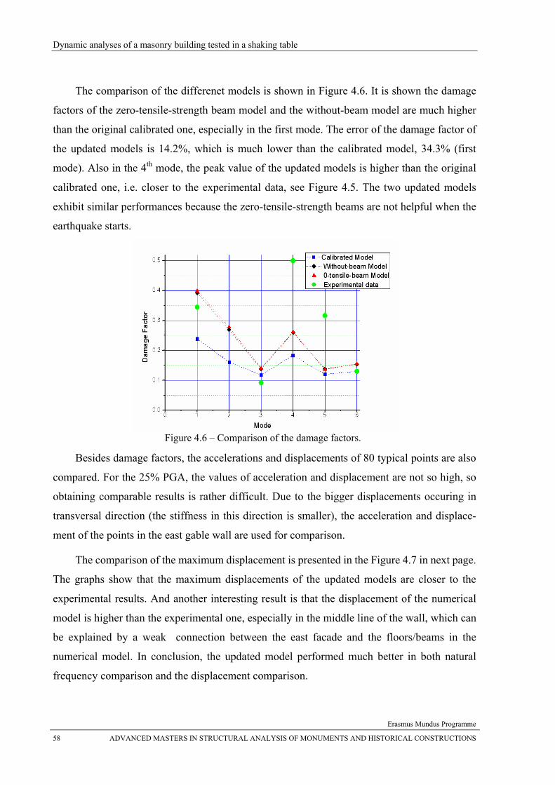
Dynamic analyses of a masonry building tested in a shaking table
Erasmus Mundus Programme
58 ADVANCED MASTERS IN STRUCTURAL ANALYSIS OF MONUMENTS AND HISTORICAL CONSTRUCTIONS
The comparison of the differenet models is shown in Figure 4.6. It is shown the damage
factors of the zero-tensile-strength beam model and the without-beam model are much higher
than the original calibrated one, especially in the first mode. The error of the damage factor of
the updated models is 14.2%, which is much lower than the calibrated model, 34.3% (first
mode). Also in the 4th mode, the peak value of the updated models is higher than the original
calibrated one, i.e. closer to the experimental data, see Figure 4.5. The two updated models
exhibit similar performances because the zero-tensile-strength beams are not helpful when the
earthquake starts.
Figure 4.6 – Comparison of the damage factors.
Besides damage factors, the accelerations and displacements of 80 typical points are also
compared. For the 25% PGA, the values of acceleration and displacement are not so high, so
obtaining comparable results is rather difficult. Due to the bigger displacements occuring in
transversal direction (the stiffness in this direction is smaller), the acceleration and displace-
ment of the points in the east gable wall are used for comparison.
The comparison of the maximum displacement is presented in the Figure 4.7 in next page.
The graphs show that the maximum displacements of the updated models are closer to the
experimental results. And another interesting result is that the displacement of the numerical
model is higher than the experimental one, especially in the middle line of the wall, which can
be explained by a weak connection between the east facade and the floors/beams in the
numerical model. In conclusion, the updated model performed much better in both natural
frequency comparison and the displacement comparison.
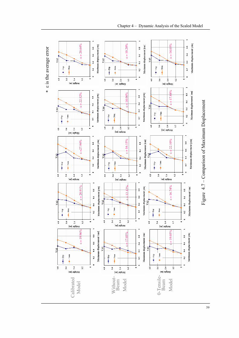
Chapter 4 – Dynamic Analysis of the Scaled Model
59
With
out-
Bea
m
Mod
el
0-Te
nsile
-B
eam
M
odel
Cal
ibra
ted
Mod
el
Figu
re 4
.7 –
Com
paris
on o
f Max
imum
Dis
plac
emen
t
is th
e av
erag
e er
ror
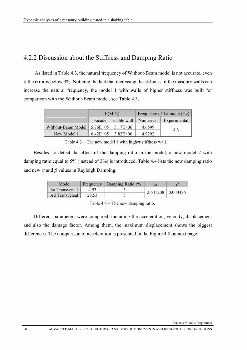
Dynamic analyses of a masonry building tested in a shaking table
Erasmus Mundus Programme
60 ADVANCED MASTERS IN STRUCTURAL ANALYSIS OF MONUMENTS AND HISTORICAL CONSTRUCTIONS
4.2.2 Discussion about the Stiffness and Damping Ratio
As listed in Table 4.3, the natural frequency of Without-Beam model is not accurate, even
if the error is below 3%. Noticing the fact that increasing the stiffness of the masonry walls can
increase the natural frequency, the model 1 with walls of higher stiffness was built for
comparison with the Without-Beam model, see Table 4.3.
E(MPa) Frequency of 1st mode (Hz) Facade Gable wall Numerical Experimental
Without-Beam Model 5.76E+05 3.17E+06 4.6599 New Model 1 6.42E+05 3.82E+06 4.9292
4.3
Table 4.3 – The new model 1 with higher stiffness wall.
Besides, to detect the effect of the damping ratio in the model, a new model 2 with
damping ratio equal to 5% (instead of 3%) is introduced, Table 4.4 lists the new damping ratio
and new α and β values in Rayleigh Damping.
Mode Frequency Damping Ratio (%) α β 1st Transversal 4.93 5 3rd Transversal 28.53 5 2.641208 0.000476
Table 4.4 – The new damping ratio.
Different parameters were compared, including the acceleration, velocity, displacement
and also the damage factor. Among them, the maximum displacement shows the biggest
differences. The comparison of acceleration is presented in the Figure 4.8 on next page.
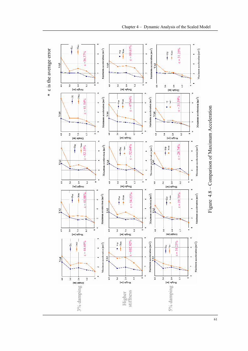
Hig
her
stiff
ness
5% d
ampi
ng
3% d
ampi
ng
Figu
re 4
.8 –
Com
paris
on o
f Max
imum
Acc
eler
atio
n
is th
e av
erag
e er
ror
Chapter 4 – Dynamic Analysis of the Scaled Model
61
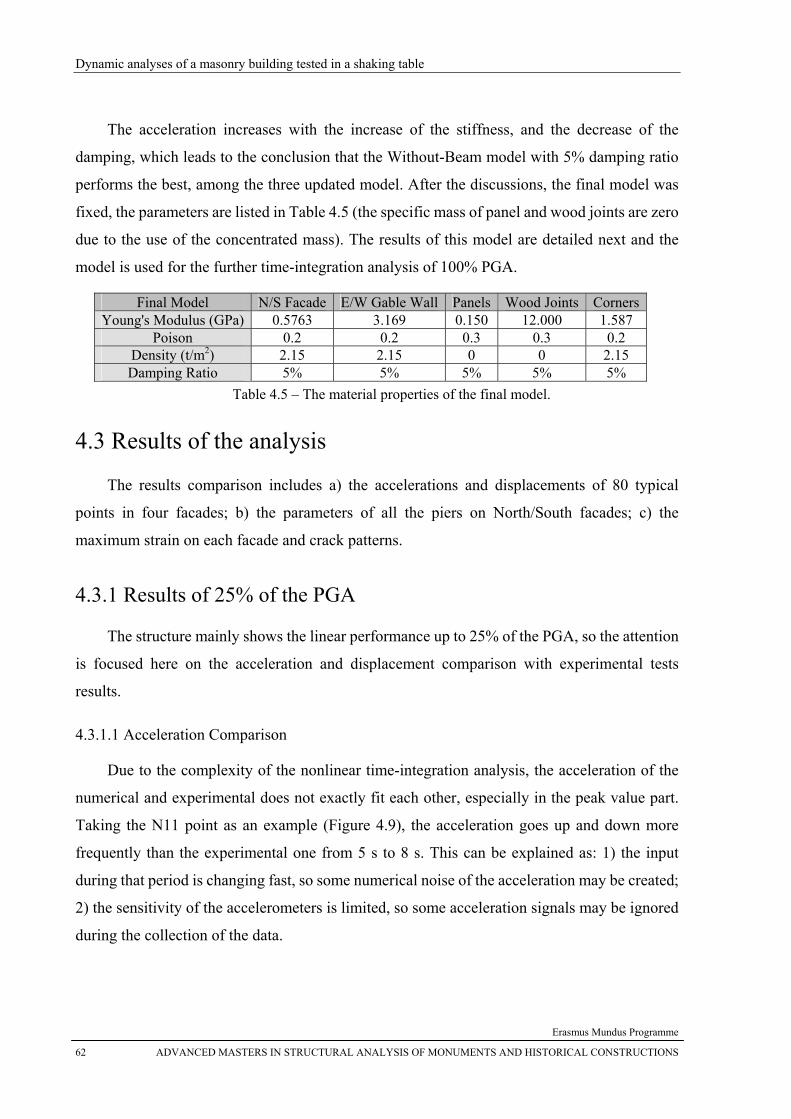
Dynamic analyses of a masonry building tested in a shaking table
Erasmus Mundus Programme
62 ADVANCED MASTERS IN STRUCTURAL ANALYSIS OF MONUMENTS AND HISTORICAL CONSTRUCTIONS
The acceleration increases with the increase of the stiffness, and the decrease of the
damping, which leads to the conclusion that the Without-Beam model with 5% damping ratio
performs the best, among the three updated model. After the discussions, the final model was
fixed, the parameters are listed in Table 4.5 (the specific mass of panel and wood joints are zero
due to the use of the concentrated mass). The results of this model are detailed next and the
model is used for the further time-integration analysis of 100% PGA.
Final Model N/S Facade E/W Gable Wall Panels Wood Joints Corners Young's Modulus (GPa) 0.5763 3.169 0.150 12.000 1.587
Poison 0.2 0.2 0.3 0.3 0.2 Density (t/m2) 2.15 2.15 0 0 2.15 Damping Ratio 5% 5% 5% 5% 5%
Table 4.5 – The material properties of the final model.
4.3 Results of the analysis
The results comparison includes a) the accelerations and displacements of 80 typical
points in four facades; b) the parameters of all the piers on North/South facades; c) the
maximum strain on each facade and crack patterns.
4.3.1 Results of 25% of the PGA
The structure mainly shows the linear performance up to 25% of the PGA, so the attention
is focused here on the acceleration and displacement comparison with experimental tests
results.
4.3.1.1 Acceleration Comparison
Due to the complexity of the nonlinear time-integration analysis, the acceleration of the
numerical and experimental does not exactly fit each other, especially in the peak value part.
Taking the N11 point as an example (Figure 4.9), the acceleration goes up and down more
frequently than the experimental one from 5 s to 8 s. This can be explained as: 1) the input
during that period is changing fast, so some numerical noise of the acceleration may be created;
2) the sensitivity of the accelerometers is limited, so some acceleration signals may be ignored
during the collection of the data.
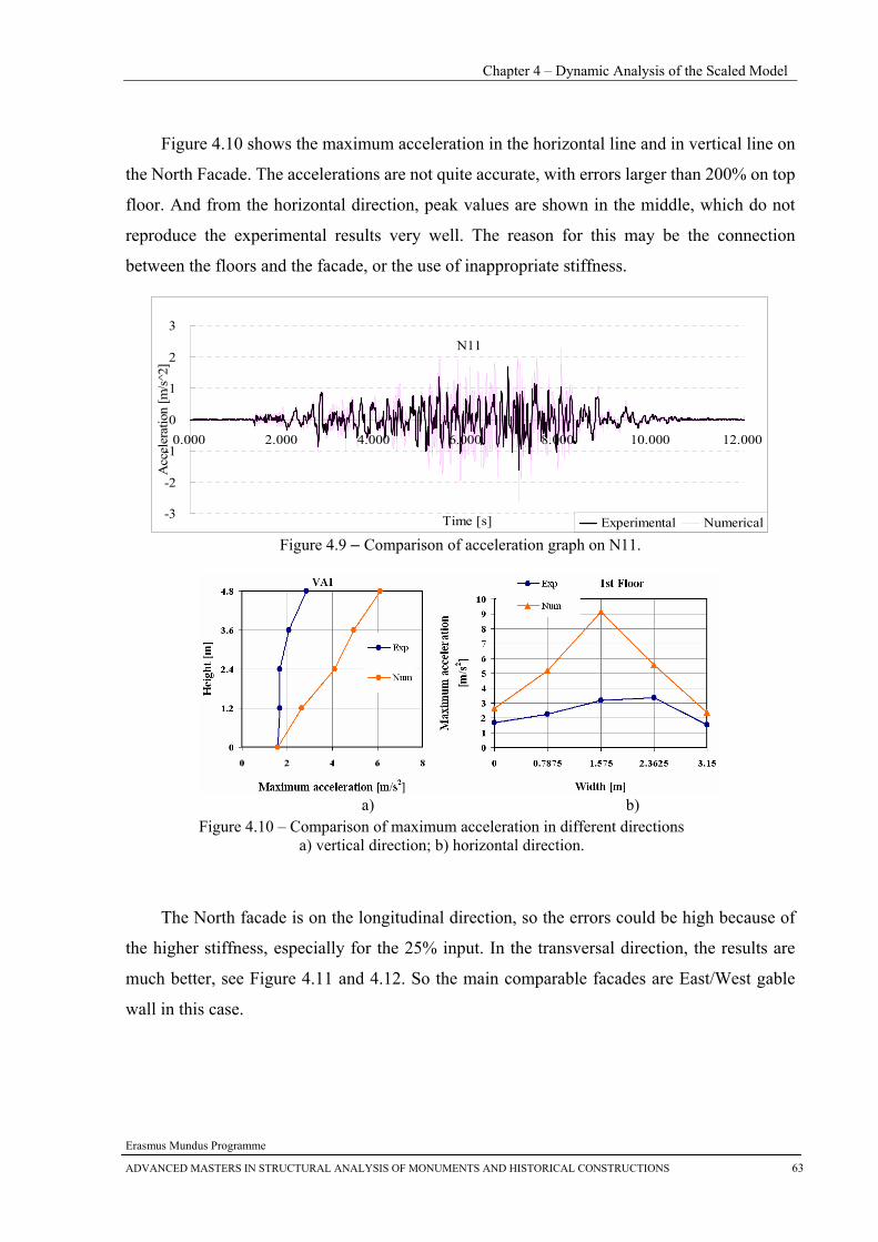
Chapter 4 – Dynamic Analysis of the Scaled Model
Erasmus Mundus Programme
ADVANCED MASTERS IN STRUCTURAL ANALYSIS OF MONUMENTS AND HISTORICAL CONSTRUCTIONS 63
Figure 4.10 shows the maximum acceleration in the horizontal line and in vertical line on
the North Facade. The accelerations are not quite accurate, with errors larger than 200% on top
floor. And from the horizontal direction, peak values are shown in the middle, which do not
reproduce the experimental results very well. The reason for this may be the connection
between the floors and the facade, or the use of inappropriate stiffness.
N11
-3
-2
-1
0
1
2
3
0.000 2.000 4.000 6.000 8.000 10.000 12.000
Time [s]
Acc
eler
atio
n [m
/s^2
]
Experimental Numerical Figure 4.9 – Comparison of acceleration graph on N11.
a) b)
Figure 4.10 – Comparison of maximum acceleration in different directions a) vertical direction; b) horizontal direction.
The North facade is on the longitudinal direction, so the errors could be high because of
the higher stiffness, especially for the 25% input. In the transversal direction, the results are
much better, see Figure 4.11 and 4.12. So the main comparable facades are East/West gable
wall in this case.
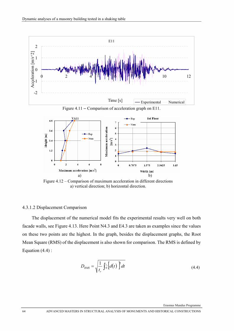
Dynamic analyses of a masonry building tested in a shaking table
Erasmus Mundus Programme
64 ADVANCED MASTERS IN STRUCTURAL ANALYSIS OF MONUMENTS AND HISTORICAL CONSTRUCTIONS
E11
-2
-1
0
1
2
0 2 4 6 8 10 12
Time [s]
Acc
eler
atio
n [m
/s^2
]
Experimental Numerical Figure 4.11 – Comparison of acceleration graph on E11.
a) b)
Figure 4.12 – Comparison of maximum acceleration in different directions a) vertical direction; b) horizontal direction.
4.3.1.2 Displacement Comparison
The displacement of the numerical model fits the experimental results very well on both
facade walls, see Figure 4.13. Here Point N4.3 and E4.3 are taken as examples since the values
on these two points are the highest. In the graph, besides the displacement graphs, the Root
Mean Square (RMS) of the displacement is also shown for comparison. The RMS is defined by
Equation (4.4) :
( )[ ] dttdt
D rt
rRMS
2
01
∫= (4.4)
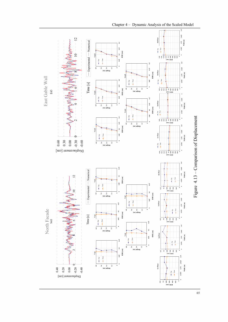
Figu
re 4
.13
–C
ompa
rison
of D
ispl
acem
ent
N43
-0.4
0
-0.2
0
0.00
0.20
0.40
02
46
810
12
Tim
e [s
]
Displacement [cm]
Expe
rimen
tal
Num
eric
al
E43
-0.6
0-0
.30
0.00
0.30
0.60
02
46
810
12
Tim
e [s
]
Displacement [cm]
Expe
rimen
tal
Num
eric
al
VA
1
0
1.2
2.4
3.6
4.8
00.
050.
10.
15
RM
S [c
m]
Height [m]
Exp
Num
VA
2
0
1.2
2.4
3.6
4.8
00.
050.
10.
15
RM
S [c
m]
Height [m]
Exp
Num
VA
3
0
1.2
2.4
3.6
4.8
00.
050.
10.
15
RM
S [c
m]
Height [m]
Exp
Num
VA
4
0
1.2
2.4
3.6
4.8
00.
050.
10.
15
RM
S [c
m]
Height [m]
Exp
Num
VA
5
0
1.2
2.4
3.6
4.8
00.
050.
10.
15
RM
S [c
m]
Height [m]
Exp
Num
2nd
Floo
r
0
0.02
0.04
0.06
0.080.1
0.12
00.
7875
1.57
52.
3625
3.15
Wid
th [m
]
RMS [cm]
Exp
Num
3rd
Floo
r
0
0.02
0.04
0.06
0.080.1
0.12
00.
7875
1.57
52.
3625
3.15
Wid
th [m
]
RMS [cm]
Exp
Num
4th
Floo
r
0
0.02
0.04
0.06
0.080.1
0.12
00.
7875
1.57
52.
3625
3.15
Wid
th [m
]
RMS [cm]
Exp
Num
1st F
loor
0
0.02
0.04
0.06
0.080.
1
0.12
00.
7875
1.57
52.
3625
3.15
Wid
th [m
]
RMS [cm]
Exp
Num
VA
11
0
1.2
2.4
3.6
4.8
00.
050.
10.
150.
2
RM
S [c
m]
Height [m]
Exp
Num
VA
12
0
1.2
2.4
3.6
4.8
00.
050.
10.
150.
2
RM
S [c
m]
Height [m]
Exp
Num
VA
13
0
1.2
2.4
3.6
4.8
00.
050.
10.
150.
2
RM
S [c
m]
Height [m]
Exp
Num
VA
14
0
1.2
2.4
3.6
4.8
00.
050.
10.
150.
2
RM
S [c
m]
Height [m]
Exp
Num
VA
15
0
1.2
2.4
3.6
4.8
00.
050.
10.
150.
2
RM
S [c
m]
Height [m]
Exp
Num
1st F
loor
00.
02
0.04
0.06
0.080.1
0.12
0.14
0.16
0.18
00.
7875
1.57
52.3
625
3.15
Wid
th [m
]
RMS [cm]
Exp
Num
2nd
Floo
r
0
0.02
0.04
0.06
0.08
0.1
0.12
0.14
0.16
0.18
00.
7875
1.57
52.
3625
3.15
Wid
th [m
]
RMS [cm]
Exp
Num
3rd
Floo
r
0
0.02
0.04
0.06
0.08
0.1
0.12
0.14
0.16
0.18
00.
7875
1.57
52.
3625
3.15
Wid
th [m
]
RMS [cm]
Exp
Num
4th
Floo
r
0
0.02
0.04
0.06
0.080.1
0.12
0.14
0.16
0.18
00.
7875
1.57
52.
3625
3.15
Wid
th [m
]
RMS [cm]
Exp
Num
Nor
th F
acad
eEa
st G
able
Wal
l
Chapter 4 – Dynamic Analysis of the Scaled Model
65
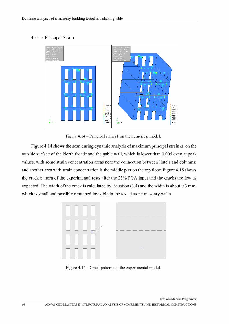
Dynamic analyses of a masonry building tested in a shaking table
Erasmus Mundus Programme
66 ADVANCED MASTERS IN STRUCTURAL ANALYSIS OF MONUMENTS AND HISTORICAL CONSTRUCTIONS
4.3.1.3 Principal Strain
Figure 4.14 – Principal stain ε1 on the numerical model.
Figure 4.14 shows the scan during dynamic analysis of maximum principal strain ε1 on the
outside surface of the North facade and the gable wall, which is lower than 0.005 even at peak
values, with some strain concentration areas near the connection between lintels and columns;
and another area with strain concentration is the middle pier on the top floor. Figure 4.15 shows
the crack pattern of the experimental tests after the 25% PGA input and the cracks are few as
expected. The width of the crack is calculated by Equation (3.4) and the width is about 0.3 mm,
which is small and possibly remained invisible in the tested stone masonry walls
Figure 4.14 – Crack patterns of the experimental model.
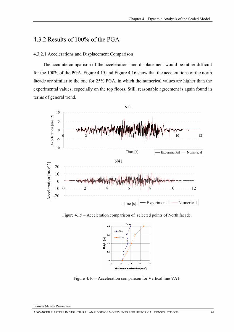
Chapter 4 – Dynamic Analysis of the Scaled Model
Erasmus Mundus Programme
ADVANCED MASTERS IN STRUCTURAL ANALYSIS OF MONUMENTS AND HISTORICAL CONSTRUCTIONS 67
4.3.2 Results of 100% of the PGA
4.3.2.1 Accelerations and Displacement Comparison
The accurate comparison of the accelerations and displacement would be rather difficult
for the 100% of the PGA. Figure 4.15 and Figure 4.16 show that the accelerations of the north
facade are similar to the one for 25% PGA, in which the numerical values are higher than the
experimental values, especially on the top floors. Still, reasonable agreement is again found in
terms of general trend.
N11
-10
-5
0
5
10
0 2 4 6 8 10 12
Time [s]
Acc
eler
atio
n [m
/s^2
]
Experimental Numerical N41
-20-10
01020
0 2 4 6 8 10 12
Time [s]
Acc
eler
atio
n [m
/s^2
]
Experimental Numerical
Figure 4.15 – Acceleration comparison of selected points of North facade.
Figure 4.16 – Acceleration comparison for Vertical line VA1.
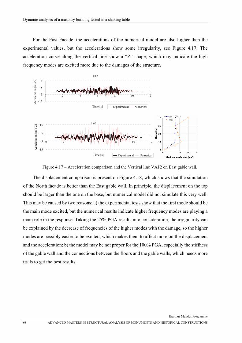
Dynamic analyses of a masonry building tested in a shaking table
Erasmus Mundus Programme
68 ADVANCED MASTERS IN STRUCTURAL ANALYSIS OF MONUMENTS AND HISTORICAL CONSTRUCTIONS
For the East Facade, the accelerations of the numerical model are also higher than the
experimental values, but the accelerations show some irregularity, see Figure 4.17. The
acceleration curve along the vertical line show a “Z” shape, which may indicate the high
frequency modes are excited more due to the damages of the structure.
E12
-15
-5
5
15
0 2 4 6 8 10 12
Time [s]
Acc
eler
atio
n [m
/s^2
]
Experimental Numerical
E42
-15
-5
5
15
0 2 4 6 8 10 12
Time [s]
Acc
eler
atio
n [m
/s^2
]
Experimental Numerical
Figure 4.17 – Acceleration comparison and the Vertical line VA12 on East gable wall.
The displacement comparison is present on Figure 4.18, which shows that the simulation
of the North facade is better than the East gable wall. In principle, the displacement on the top
should be larger than the one on the base, but numerical model did not simulate this very well.
This may be caused by two reasons: a) the experimental tests show that the first mode should be
the main mode excited, but the numerical results indicate higher frequency modes are playing a
main role in the response. Taking the 25% PGA results into consideration, the irregularity can
be explained by the decrease of frequencies of the higher modes with the damage, so the higher
modes are possibly easier to be excited, which makes them to affect more on the displacement
and the acceleration; b) the model may be not proper for the 100% PGA, especially the stiffness
of the gable wall and the connections between the floors and the gable walls, which needs more
trials to get the best results.
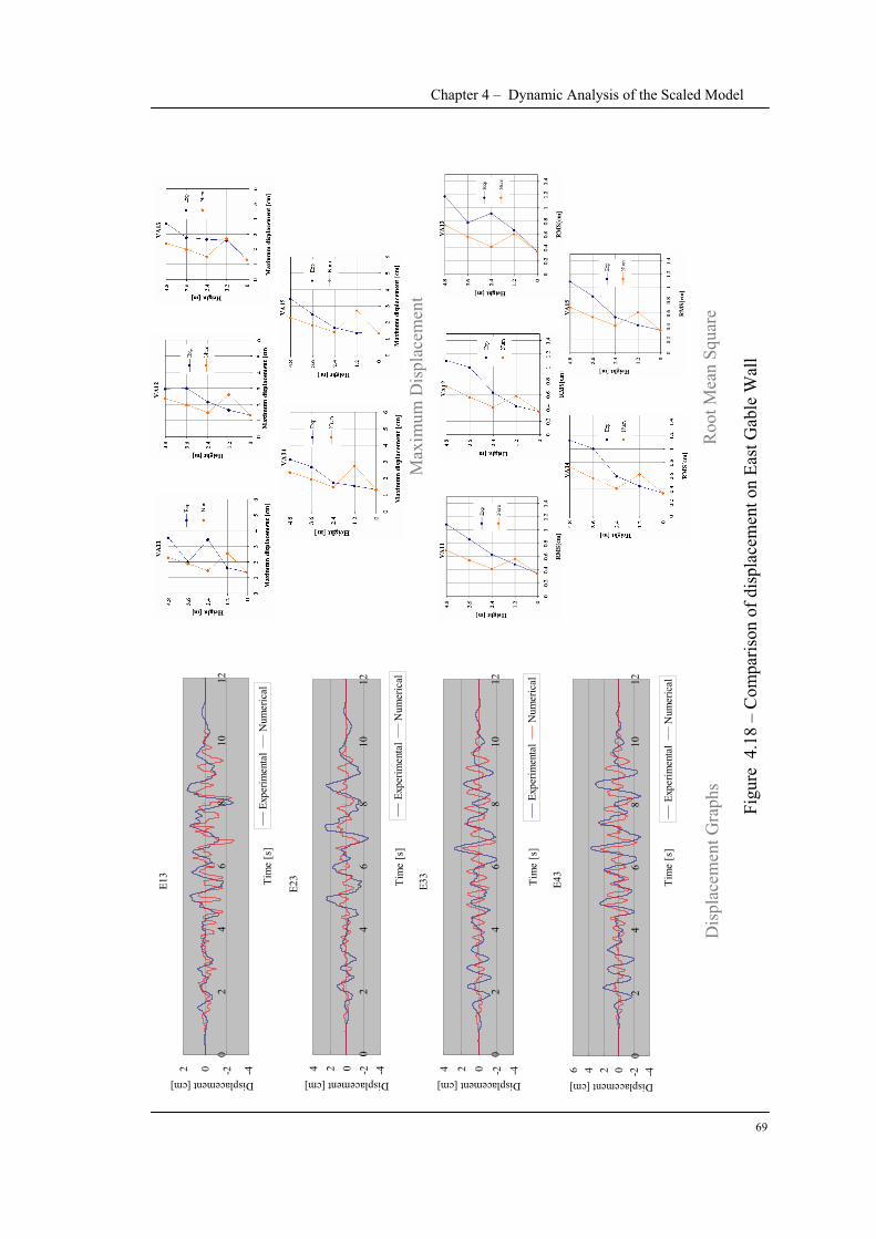
Chapter 4 – Dynamic Analysis of the Scaled Model
69
Figu
re 4
.18
–C
ompa
rison
of d
ispl
acem
ent o
n Ea
st G
able
Wal
l
Dis
plac
emen
t Gra
phs
E13
-4-202
02
46
810
12
Tim
e [s
]
Displacement [cm]
Expe
rimen
tal
Num
eric
al
E23
-4-2024
02
46
810
12
Tim
e [s
]
Displacement [cm]
Expe
rimen
tal
Num
eric
al
E33
-4-2024
02
46
810
12
Tim
e [s
]
Displacement [cm]
Expe
rimen
tal
Num
eric
al
E43
-4-20246
02
46
810
12
Tim
e [s
]
Displacement [cm]
Expe
rimen
tal
Num
eric
al
Roo
t Mea
n Sq
uare
Max
imum
Dis
plac
emen
t
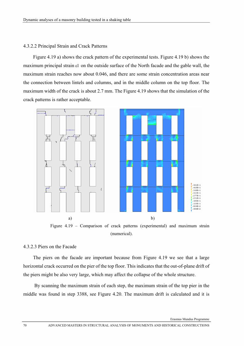
Dynamic analyses of a masonry building tested in a shaking table
Erasmus Mundus Programme
70 ADVANCED MASTERS IN STRUCTURAL ANALYSIS OF MONUMENTS AND HISTORICAL CONSTRUCTIONS
4.3.2.2 Principal Strain and Crack Patterns
Figure 4.19 a) shows the crack pattern of the experimental tests. Figure 4.19 b) shows the
maximum principal strain ε1 on the outside surface of the North facade and the gable wall, the
maximum strain reaches now about 0.046, and there are some strain concentration areas near
the connection between lintels and columns, and in the middle column on the top floor. The
maximum width of the crack is about 2.7 mm. The Figure 4.19 shows that the simulation of the
crack patterns is rather acceptable.
a) b)
Figure 4.19 – Comparison of crack patterns (experimental) and maximum strain
(numerical).
4.3.2.3 Piers on the Facade
The piers on the facade are important because from Figure 4.19 we see that a large
horizontal crack occurred on the pier of the top floor. This indicates that the out-of-plane drift of
the piers might be also very large, which may affect the collapse of the whole structure.
By scanning the maximum strain of each step, the maximum strain of the top pier in the
middle was found in step 3388, see Figure 4.20. The maximum drift is calculated and it is
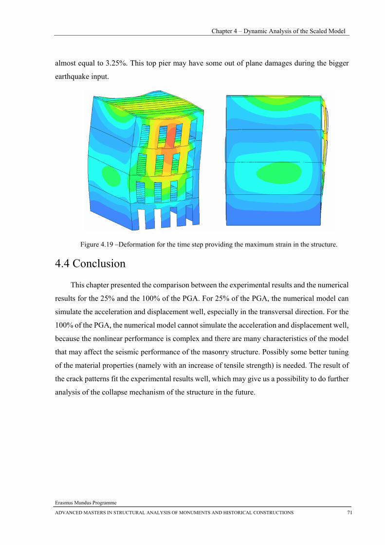
Chapter 4 – Dynamic Analysis of the Scaled Model
Erasmus Mundus Programme
ADVANCED MASTERS IN STRUCTURAL ANALYSIS OF MONUMENTS AND HISTORICAL CONSTRUCTIONS 71
almost equal to 3.25%. This top pier may have some out of plane damages during the bigger
earthquake input.
Figure 4.19 –Deformation for the time step providing the maximum strain in the structure.
4.4 Conclusion
This chapter presented the comparison between the experimental results and the numerical
results for the 25% and the 100% of the PGA. For 25% of the PGA, the numerical model can
simulate the acceleration and displacement well, especially in the transversal direction. For the
100% of the PGA, the numerical model cannot simulate the acceleration and displacement well,
because the nonlinear performance is complex and there are many characteristics of the model
that may affect the seismic performance of the masonry structure. Possibly some better tuning
of the material properties (namely with an increase of tensile strength) is needed. The result of
the crack patterns fit the experimental results well, which may give us a possibility to do further
analysis of the collapse mechanism of the structure in the future.

Dynamic analyses of a masonry building tested in a shaking table
Erasmus Mundus Programme
72 ADVANCED MASTERS IN STRUCTURAL ANALYSIS OF MONUMENTS AND HISTORICAL CONSTRUCTIONS
Chapter 5 – Dynanmic Analysis of the Full Scale Model
Erasmus Mundus Programme
ADVANCED MASTERS IN STRUCTURAL ANALYSIS OF MONUMENTS AND HISTORICAL CONSTRUCTIONS 73
CChhaapptteerr 55
DDyynnaammiicc AAnnaallyyssiiss ooff tthhee FFuullll SSccaallee MMooddeell
Abstract In this chapter, issues about the scale factor in this shaking table tests of masonry structures will be presented. As addressed in Chapter 3, more gravity should have been taken into account in the 1:3 models tested in the shaking table. Therefore, a calibrated numerical full scale model will be put into nonlinear time-integration analysis to evaluate the effect of the self weight. The full scale model is again computationally tested for 25% and 100% PGA, to compare the new results with the scaled model results. In the end, some conclusions are provided.
Dynamic analyses of a masonry building tested in a shaking table
Erasmus Mundus Programme
74 ADVANCED MASTERS IN STRUCTURAL ANALYSIS OF MONUMENTS AND HISTORICAL CONSTRUCTIONS
5.1 Basic Introduction to Scaling
Testing of complete structures is normally used to enable the understanding of the global
behaviour of a construction and to capture the interplay of the response of its different
components. This provides quite realistic information on the expected response of the specific
structures under testing, but corresponds to rather expensive tests. So the scaled model tests are
often used to keep costs acceptable and allow the consideration of more testing variations. But
the due to the geometrical scaling, many laws should be respect in order to keep the same
performance between reduced models and the prototypes. In this section, a basic discussion of
size effect will be presented.
5.1.1 Effect of Size effect on Strength
Discussion about the size effect of masonry structure is expected to be similar to concrete
structures, despite the fact the masonry is a composite material with mortar and masonry units.
The fracture toughness of concrete as determined by the work-of-fracture method depends on
the size of specimens. This is the so-called size effect. It appears in all structures, but it is more
pronounced in structures made of cementitious materials due to their large fracture process
zone (FPZ), which plays a vital role in the analysis of growth of the crack. The size effect is
defined in terms of the nominal stress σN at maximum (ultimate) load of geometrically similar
structures of different sizes. The nominal stress in a structure need not to represent an actual
stress and is defined as σN = Pu/bd or σN = Pu/d2 for a two or three dimensional structure,
respectively, where d is a characteristic dimension of the structure (e.g. the depth or the span of
a beam, the length of the FPZ, etc.) and b is the thickness of the two dimensional structure. A
dependence of σN on the size of the structures called the size effect. If σN does not depend on the
size of the structure we say that there is no size effect. The size effect in concrete structures can
be easily established if we consider as characteristic length the length of the FPZ. If we consider
that this length is approximately five to six times the size of the aggregates, then the length of
the FPZ is constant, whereas the size of the structure changes (Gdoutos, 2005).
Thus, for large structures the size of the FPZ is negligible, while for small structures it is
appreciable. This explains the rather brittle behaviour of large structures, as opposed to the
ductile behaviour of small structures. Classical theories, such as elastic analysis with allowable
stress or plastic limit analysis cannot take into consideration the size effect. Contrary, linear
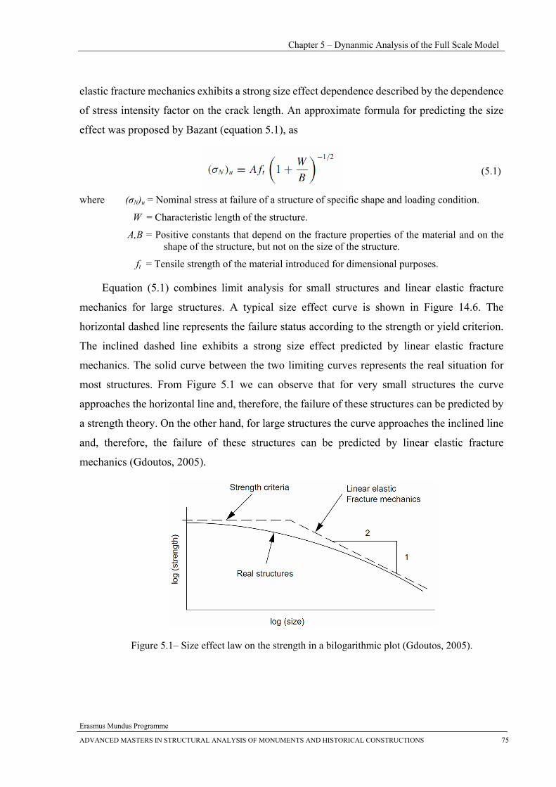
Chapter 5 – Dynanmic Analysis of the Full Scale Model
Erasmus Mundus Programme
ADVANCED MASTERS IN STRUCTURAL ANALYSIS OF MONUMENTS AND HISTORICAL CONSTRUCTIONS 75
elastic fracture mechanics exhibits a strong size effect dependence described by the dependence
of stress intensity factor on the crack length. An approximate formula for predicting the size
effect was proposed by Bazant (equation 5.1), as
(5.1)
where (σN)u = Nominal stress at failure of a structure of specific shape and loading condition.
W = Characteristic length of the structure.
A,B = Positive constants that depend on the fracture properties of the material and on the shape of the structure, but not on the size of the structure.
ft = Tensile strength of the material introduced for dimensional purposes.
Equation (5.1) combines limit analysis for small structures and linear elastic fracture
mechanics for large structures. A typical size effect curve is shown in Figure 14.6. The
horizontal dashed line represents the failure status according to the strength or yield criterion.
The inclined dashed line exhibits a strong size effect predicted by linear elastic fracture
mechanics. The solid curve between the two limiting curves represents the real situation for
most structures. From Figure 5.1 we can observe that for very small structures the curve
approaches the horizontal line and, therefore, the failure of these structures can be predicted by
a strength theory. On the other hand, for large structures the curve approaches the inclined line
and, therefore, the failure of these structures can be predicted by linear elastic fracture
mechanics (Gdoutos, 2005).
Figure 5.1– Size effect law on the strength in a bilogarithmic plot (Gdoutos, 2005).
Dynamic analyses of a masonry building tested in a shaking table
Erasmus Mundus Programme
76 ADVANCED MASTERS IN STRUCTURAL ANALYSIS OF MONUMENTS AND HISTORICAL CONSTRUCTIONS
5.1.2 Effect of Size effect on Shaking Table Tests
As introduced in Chapter 4, the maximum dimensions and payload capacity of the table
which in most cases call for the use of reduced scale specimens (typically in the range of 1:3 to
1:8 geometric scale for large shaking tables if a multi-storey structural system is to be tested).
The need for reduced scales in shaking table tests of complete structural systems is one of
the major drawbacks of this type of testing, due to the similitude problems that it raises (Okada
and Bertero et al., 1978). In fact, in order to be able to test an undistorted reinforced concrete
model to its ultimate capacity, it is necessary to obtain a true simulation of
– The geometry;
– The stress-strain relationship of the materials;
– The mass and the gravity forces;
– The initial and boundary conditions.
Geometric similitude is normally achieved by a direct application of a geometrical scale
and does not present any difficulty, besides that associated with the construction of small
specimens (Carvalho, 1998).
The accurate simulation of the stress-strain relationships is much more difficult (Bedell
and Abrams, 1982), even when using essentially the same material in the prototype and in the
model. Small geometric scales require for example the use of micro-concrete and specially
manufactured reinforcing bars or scaled masonry units. Thus, it is extremely difficult to satisfy
by scaling models, throughout the complete spectrum of stresses, strains, amplitude of load
reversals, srain rates and strain gradients. For concrete, a correct simulation of the compressive
and tensile strengths, together with the ultimate strain is of critical importance. The bond
characteristics are an important aspect conditioning the correct simulation of the structural
behaviour. In this respect a large scatter of results is to be expected, with cases being known of
superior bond behaviour of reinforced concrete structures in small scale (Abrams and
Tangkijingamvong, 1984).
The Cauchy value and Froude value are listed again, given by
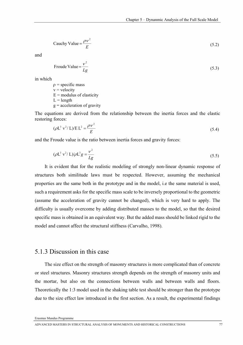
Chapter 5 – Dynanmic Analysis of the Full Scale Model
Erasmus Mundus Programme
ADVANCED MASTERS IN STRUCTURAL ANALYSIS OF MONUMENTS AND HISTORICAL CONSTRUCTIONS 77
E
2
ValueCauchy ρν= (5.2)
and
Lg
2
Value Froude ν= (5.3)
in which ρ = specific mass v = velocity E = modulus of elasticity L = length g = acceleration of gravity
The equations are derived from the relationship between the inertia forces and the elastic restoring forces:
E
2223 L L)/E/ vL( ρνρ = (5.4)
and the Froude value is the ratio between inertia forces and gravity forces:
Lgg
2323 LL)// vL( νρρ = (5.5)
It is evident that for the realistic modeling of strongly non-linear dynamic response of
structures both similitude laws must be respected. However, assuming the mechanical
properties are the same both in the prototype and in the model, i.e the same material is used,
such a requirement asks for the specific mass scale to be inversely proportional to the geometric
(assume the acceleration of gravity cannot be changed), which is very hard to apply. The
difficulty is usually overcome by adding distributed masses to the model, so that the desired
specific mass is obtained in an equivalent way. But the added mass should be linked rigid to the
model and cannot affect the structural stiffness (Carvalho, 1998).
5.1.3 Discussion in this case
The size effect on the strength of masonry structures is more complicated than of concrete
or steel structures. Masonry structures strength depends on the strength of masonry units and
the mortar, but also on the connections between walls and between walls and floors.
Theoretically the 1:3 model used in the shaking table test should be stronger than the prototype
due to the size effect law introduced in the first section. As a result, the experimental findings
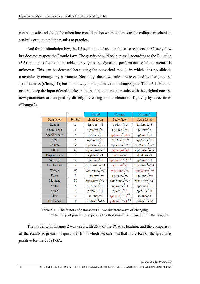
Dynamic analyses of a masonry building tested in a shaking table
Erasmus Mundus Programme
78 ADVANCED MASTERS IN STRUCTURAL ANALYSIS OF MONUMENTS AND HISTORICAL CONSTRUCTIONS
can be unsafe and should be taken into consideration when it comes to the collapse mechanism
analysis or to extend the results to practice.
And for the simulation law, the 1:3 scaled model used in this case respects the Cauchy Law,
but does not respect the Froude Law. The gravity should be increased according to the Equation
(5.3), but the effect of this added gravity to the dynamic performance of the structure is
unknown. This can be detected here using the numerical model, in which it is possible to
conveniently change any parameter. Normally, these two rules are respected by changing the
specific mass (Change 1), but in that way, the input has to be changed, see Table 5.1. Here, in
order to keep the input of earthquake and to better compare the results with the original one, the
new parameters are adopted by directly increasing the acceleration of gravity by three times
(Change 2).
Table 5.1 – The factors of parameters in two different ways of changing * The red part provides the parameters that should be changed from the original.
The model with Change 2 was used with 25% of the PGA as loading, and the comparison
of the results is given in Figure 5.2, from which we can find that the effect of the gravity is
positive for the 25% PGA.
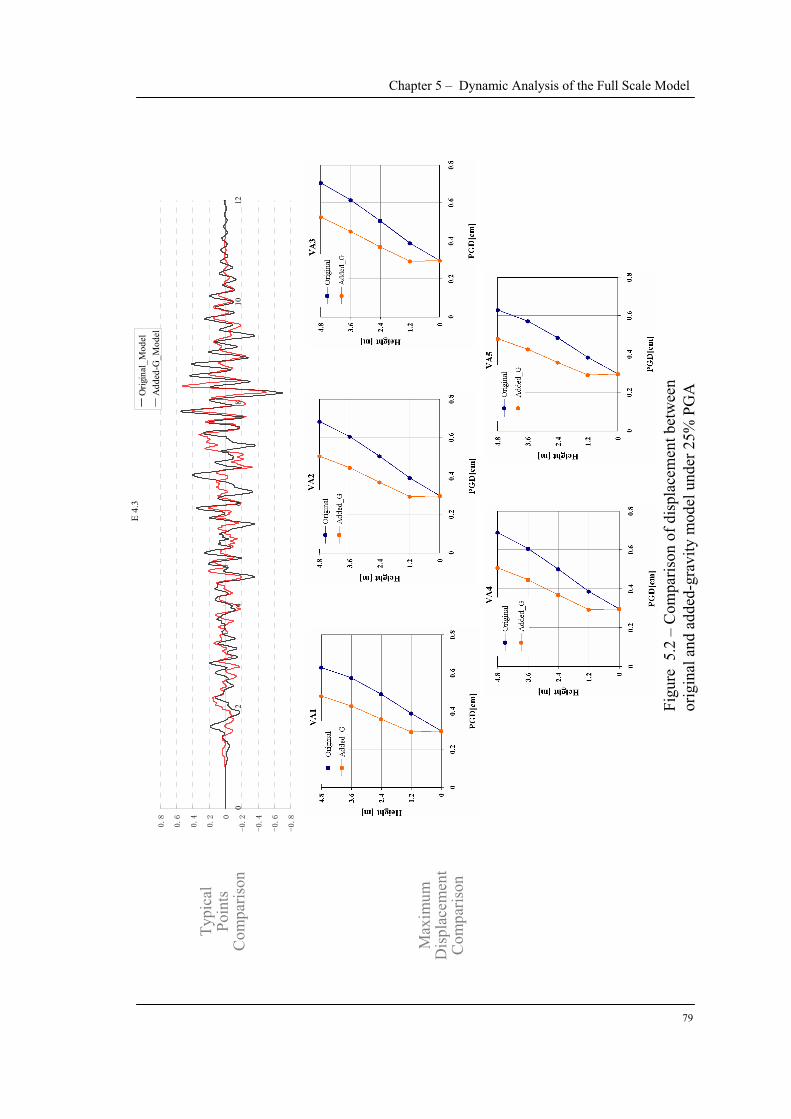
Typi
cal
Poin
tsC
ompa
rison
Chapter 5 – Dynamic Analysis of the Full Scale Model
79
Figu
re 5
.2 –
Com
paris
on o
f dis
plac
emen
t bet
wee
n or
igin
al a
nd a
dded
-gra
vity
mod
el u
nder
25%
PG
A
Max
imum
D
ispl
acem
ent
Com
paris
on
E 4.
3
02
46
810
12
Orig
inal
_Mod
elA
dded
-G_M
odel
Dynamic analyses of a masonry building tested in a shaking table
Erasmus Mundus Programme
80 ADVANCED MASTERS IN STRUCTURAL ANALYSIS OF MONUMENTS AND HISTORICAL CONSTRUCTIONS
This can be explained as the movement of the structures are small and the response is
mostly elastic, meaning that the gravity will add normal stress to the structure, which will
increase the strength for the low earthquake input. For higher input the influence remains
unclear, as compressive failure might play a rule. Due to time limitations, the 100% PGA
loading results could not be completed and cannot be shown here. It is expected that the results
are similar with the full scale tests shown below.
The damage factor in Figure 5.3 can also prove that the damage of the model with
additional gravity is smaller.
Figure 5.3 – The comparison of the damage factor between two models.
Additionally, in order to prove the correctness of the Cauchy and Froude law, the model
with added-gravity is also used to compare with the full scale model with 25% PGA loading. If
the behaviour is elastic, the displacement of the added-gravity model should be 3 times as much
as the displacement of the full scale model. Figure 5.4 indicates that the results fit very well and
the law is accurate (Examples: N1.2 and N4.2), despite the fact that some non-linearity is
present.
N12
-1.5-1.0-0.50.00.51.01.5
0 2 4 6 8 10 12
Time [s]
Dis
plac
emen
t [cm
]
3×Added-gravity model Full scale model
Chapter 5 – Dynanmic Analysis of the Full Scale Model
Erasmus Mundus Programme
ADVANCED MASTERS IN STRUCTURAL ANALYSIS OF MONUMENTS AND HISTORICAL CONSTRUCTIONS 81
N42
-1.5-1.0-0.50.00.51.01.5
0 2 4 6 8 10 12
Time [s]
Dis
plac
emen
t[cm
]
3×Added-gravity model Full scale model
Figure 5.4 – Comparison of displacement between added-gravity model
and full scale model (N1.2 and N4.2).
The added-gravity model is now running for the 100% PGA, but due to the time limitation,
this part can not be put in the dissertation, but the addition data will be put as attach at the end of
the dissertation and be presented on the defence.
5.2 Results of the Full Scale Model
As stated before, the displacements of the full scale model for 25% PGA loading are
smaller than 3 times the displacement of scaled model without added masses, which indicates
that the gravity can create a positive effect on the performance of the structures. So attention
here will mainly be focused on the comparison of the 100% PGA between these two models.
5.2.1 Displacement
The performance of the full scale model for 100% PGA is very much similar with the scale
model for 100% of the PGA. Again, the full scale model did not simulate the experimental
results very well. From the results, it is noticed that the displacement of the full scale model is
significantly smaller than the 3 times the displacement of the scaled model, see Figure 5.5.
Dynamic analyses of a masonry building tested in a shaking table
Erasmus Mundus Programme
82 ADVANCED MASTERS IN STRUCTURAL ANALYSIS OF MONUMENTS AND HISTORICAL CONSTRUCTIONS
Figure 5.5 – Comparison of Maximum Displacement between full scale and the scale model.
It is noted that the full scale model did not show a very large value on the second floor, but
instead, an almost straight line along the height, which seems to be due to the fact that far less
nonlinear behaviour is found.
5.2.2 Principal Strain and Piers Analysis
Figure 5.6 shows the maximum principal strains for the full scale model, which are smaller
than the scaled model. Table 5.2 shows the comparison of the maximum principal strain and the
slope in the middle of the top pier in the middle. It is noticed that all these values are smaller.
Figure 5.6 – Maximum principal strain of the full scale model.
Chapter 5 – Dynanmic Analysis of the Full Scale Model
Erasmus Mundus Programme
ADVANCED MASTERS IN STRUCTURAL ANALYSIS OF MONUMENTS AND HISTORICAL CONSTRUCTIONS 83
Scaled model Full scale model Maximum Strain (peak value) 0.461E-01 0.265E-01
Damage factor of 1st Mode 0.65 0.59 Damage factor of 2nd Mode 0.53 0.51 Damage factor of 3rd Mode 0.47 0.45
Maximum Slope 3.25% 1.17%
Table 5.2 – Comparison of Maximum strain, damage factors and maximum slope in two models.
Note that, all the conclusions are based on the numerical model analysis only and the same
material properties are adopted, so the results only address scaling effect. As mentioned in the
last chapter, the numerical simulation does not simulate the experimental results perfectly,
especially for the 100% PGA. So the numerical model needs to be improved to get a closer
agreement with the experiments. Still, this remark does not affect the conclusion found that not
including the additional masses and testing at reduced scale is beneficial for this structure.
5.3 Conclusion
The analyses of the full scale model are presented in this chapter. The following
conclusions can be drawn as:
· For the size effect law, the mock-up used in the shaking table tests is stronger than
the real building because of the size effect on the strength. So from this point of view,
the analysis would be more favourable than the real situation.
· However, the mock-up also needs more gravity to be added according to the Froude
Similitude Law, and the additional gravity was found to be helpful when the
earthquake happens, when compared to the absence of additional loading. By
comparing to a full scale building, which already includes size effect, it was shown
that testing a small scale building without additional masses provides a more severe
response, meaning that the obtained results are conservative and can be extrapolated
to larger sizes.

Dynamic analyses of a masonry building tested in a shaking table
Erasmus Mundus Programme
84 ADVANCED MASTERS IN STRUCTURAL ANALYSIS OF MONUMENTS AND HISTORICAL CONSTRUCTIONS

Chapter 6 –Conclusions and the Future Works
Erasmus Mundus Programme
ADVANCED MASTERS IN STRUCTURAL ANALYSIS OF MONUMENTS AND HISTORICAL CONSTRUCTIONS 85
CChhaapptteerr 66
CCoonncclluussiioonnss aanndd tthhee FFuuttuurree WWoorrkkss

Dynamic analyses of a masonry building tested in a shaking table
Erasmus Mundus Programme
86 ADVANCED MASTERS IN STRUCTURAL ANALYSIS OF MONUMENTS AND HISTORICAL CONSTRUCTIONS
6.1 Conclusions
This dissertation addresses the basic experimental and numerical methods in earthquake
engineering, focusing with detail on the seismic assessment of masonry “Gaioleiro” buildings,
and performing numerical modeling using nonlinear time-integration analyses and comparing
the results to the data obtained from the previous testing. The comparison includes the
displacement and acceleration on 80 typical points on the structure, the damage indicator after
each earthquake input and the crack patterns. Furthermore, an updated full scale numerical
model is also used for the nonlinear time-integration analyses with the objective of discussing
the scaling in dynamic analysis.
The conclusions of the whole dissertation can be summerized as:
· Scaled model: According to the comparison between the experimental results and
the numerical results for the 25% and the 100% of the PGA, the numerical model
can simulate the acceleration and displacement well, especially in the transversal
direction. For the 100% of the PGA, the numerical model cannot simulate the
acceleration and displacement well, because the nonlinear performance is complex
and there are many characteristics of the model that may affect the seismic
performance of the masonry structure. Possibly some better tuning of the material
properties (namely with an increase of tensile strength) is needed. The result of the
crack patterns fit the experimental results well, which may give us a possibility to
do further analysis of the collapse mechanism of the structure in the future.
· Full Scale model: For the size effect law, the mock-up used in the shaking table
tests is stronger than the real building because of the size effect on the strength. So
from this point of view, the analysis would be more favourable than the real
situation. However, the mock-up also needs more gravity to be added according to
the Froude Similitude Law, and the additional gravity was found to be helpful when
the earthquake happens, when compared to the absence of additional loading. By
comparing to a full scale building, which already includes size effect, it was shown
that testing a small scale building without additional masses provides a more severe
response, meaning that the obtained results are conservative and can be
extrapolated to larger sizes.
Chapter 6 –Conclusions and the Future Works
Erasmus Mundus Programme
ADVANCED MASTERS IN STRUCTURAL ANALYSIS OF MONUMENTS AND HISTORICAL CONSTRUCTIONS 87
6.2 Future Works
Due to the time limitation, several possible trials that may improve the numerical model
could not be made. The future work to be done may include:
· Model Optimazition: As stated in the conclusions, the numerical model is not
perfect. The possible improvement could be: a) changing the connections between
the floors and the masonry walls, especially the gable walls. The comparison of the
acceleration and displacement shows the numerical results are larger than the
experimental results; b) increasing the stiffness of the gable walls. And the natural
frequencies may increase by increasing the stiffness, which may improve the results
of the 100% of the PGA; c) increasing the tensile strength of the masonry; d)
Newton-Raphson Method is adopted in this dissertation, in which the stiffness
matrices need to be updated before every iteration. The calculation time for the
scale model of 100% PGA load is about one week, and some steps did not converge.
Other iteration methods could be adopted to compare.
· Collapse Mechanism: Collapse mechanism is an important aspect of the masonry
dynamic analyses. In the dissertation, no such issues are addressed. Future work
can be done by increasing the input of the earthquake and analyzing the possible
collapse mechanism of the structures. The attention should be focused on the
out-of-plane mechanism of the piers on the North/South facades.
· Size Effect on the Strength of Masonry: In this dissertation, the full model was
used to detect the effect of the scaling in the shaking table tests, but the size effect
on the strength of masonry is not taken into consideration. Further analyses could
be made to discuss this issue.

Dynamic analyses of a masonry building tested in a shaking table
Erasmus Mundus Programme
88 ADVANCED MASTERS IN STRUCTURAL ANALYSIS OF MONUMENTS AND HISTORICAL CONSTRUCTIONS
References
Erasmus Mundus Programme
ADVANCED MASTERS IN STRUCTURAL ANALYSIS OF MONUMENTS AND HISTORICAL CONSTRUCTIONS 89
RReeffeerreenncceess
A
Arams, D.P.; Tangkijingamvong, S. (1984): Dynamic response of reduced scale models
and reinforced concrete structures. Proc. 8th World Conf. On Earthq. Engng. Vol
VI, 371-378, San Francisco
Aktan, A.E.; Bertero, V.V. (1984): Earthquake response of a 1/5th scale model of a 7-story
reinforced concrete frame-wall structure system. Proc. 8th World Conf. On Earthq.
Engng, Vol VI,651-658, San Francisco
B
Bairrao, R.; Falcao Silva M.J.; Juhasova, E.; Campos-Costa A.; Coelho, E.(2006):
Shaking table tests on an asymmetric limestone building, First European
Conference on Earthquake Engineering and Seismology, 536, Geneva,
Switzerland, 3-8, September 2006
Barbat, A.H.; Pujades, L.G.; Lantada,N. (2006): Performance of buildings under earth-
quakes in Barcelona, Spain, Computer-Aided Civil and Infrastructure
Engineering 21, 573–593
Bazant, Z.P. (1983): Fracture in Concrete and reinforced concrete, IUTAM Prager Symp.
on Mechanics of Geomaterials: Rocks, Concretes, Soils. Z. P. Bazant, ed.,
Northwester Univ., Evanston, I II., 281-361 (Eq. 16)
Bazant, Z.P. (1984): Size effect in blunt fracture: concrete, rock, metal. J. of Engrg. Mech.,
ASCE, 110, 518-535
Bazant, Z.P.; Xi, Y. (1991): Statistical size effect in quasi-brittle structures: II. Nonlocal
theory. J Engrg. Mech., ASCE, 117(11), 2623-2640
Dynamic analyses of a masonry building tested in a shaking table
Erasmus Mundus Programme
90 ADVANCED MASTERS IN STRUCTURAL ANALYSIS OF MONUMENTS AND HISTORICAL CONSTRUCTIONS
Bazant, Z.P. (2002): Scaling of Structural Strength, Hermes Penton Ltd, 2002, 33-38,
165-174
Bedell, R.J.; Abrams, D.P. (1983): Scale relationships of concrete columns. Res. Series
83-02. Dept. of Civil, Environmental and Architectural Engineering, University
of Colorado, Boulder, Colorado
Benedetti, D.; Carydis, P.; Pezzoli, P. (1998): Shaking table tests on 24 simple masonry
buildings, Earthquake Engineering and Structural Dynamics 27, 67–90
C
Candeias, P.; Costa, A.C.; Coelho, E.(2004): Shaking table tests of 1:3 reduced scale
models of four story unreinforced masonry buildings, Proc.of the13th World
Conference on Earthquake Engineering, Vancouver, Canada
Carvalho, E.C.(1998): Seismic testing of structures, Proc.ofthe11th European Conference
on Earthquake, Paris, France. Rotterdam: AABalkema
Casarotti, C.; Pinho, R. (2007): An adaptive spectrum method for assessment of bridges
subjected to earthquake action, Bulletin of Earthquake Engineering 3, 377–390
Cervera, M.; Oliver, J.; Faria, R. (1995): Seismic evaluation of concrete dams via
continuum damage models, Earthquake Engineering and Structural Dynamics 24,
1225–1245
Chopra, A.K. (2000): Dynamic of Structures – Theory and Applications to Earthquake
Engineering, Prentice Hall, Englewood Cliffs, NJ
Chopra, A.K.; Goel, R.K. (2002): A modal pushover analysis procedure for estimating
seismic demands for buildings, Earthquake Engineering and Structural Dynamics
21, 561–582
Clough, R.W.; Penzien J. (1995): Dynamics of Structures, Third Edition, Computers and
Structures, Inc
References
Erasmus Mundus Programme
ADVANCED MASTERS IN STRUCTURAL ANALYSIS OF MONUMENTS AND HISTORICAL CONSTRUCTIONS 91
D
DIANA (2008) DIsplacement method ANAlyser. Release 9.4, Cd-rom, Netherlands
Douglas, B.M.; Reid, W.H. (1982); Dynamic tests and system identification of bridges,
Structural Division, ASCE 108, 2295–2313
E
EN1996-1(2004): Eurocode 6: Design of masonry structures
EN1998-1(2004): Eurocode 8: Design of structures for earthquake resistance – General
rules, seismic actions and rules for buildings
G
Gdoutos, E.E., (2005): Fracture Mechanics, second edition, pp. 353-365, Springer
Gelfi, P. (2006): SIMQKE_GR–Artificial earthquakes compatible with response spectra,
University of Brescia, Italy
Gulkan, P., Aschheim, M.; Spence, R. (2002): Reinforced concrete frame buildings with
masonry infills, World Housing Encyclopedia, Housing report: 64. Available
from www.world-housing.net
M
Mendes, N.; Lourenço, P.B. (2008): Reduction of the seismic vulnerability of ancient
buildings, Activity report of project POCI/ECM/61671/2004, FCT (in
Portuguese), Available from www.civil.uminho.pt/masonry
O
Oliveira, C.S. (2003): Seismic vulnerability of Historical Constructions: A Contribution,
Bulletin of Earthquake Engineering 1: 37-82, 2003
Oliveira, D.V. (2003): Experimental and Numerical Analysis of Blocky Masonry
Structures Under Cyclic Loading, PhD Thesis, Universidade do Minho, 211 p.
(www.civil.uminho.pt/masonry)
Dynamic analyses of a masonry building tested in a shaking table
Erasmus Mundus Programme
92 ADVANCED MASTERS IN STRUCTURAL ANALYSIS OF MONUMENTS AND HISTORICAL CONSTRUCTIONS
Oliveira, D.V. (2004): Reduction of the risk seismic and implications in the real state,
Proc.of the 6th National Congress of Seismology and Earthquake Engineering
2004, Special session. Available from www.civil.uminho.pt/masonry
P
Pinho, F.F. (2000): Walls from ancient Portuguese buildings, ‘‘Edifıcios,’’ n 8, LNEC (In
Portuguese)
Paquette, J.; Bruneau, M. (2004): Pseudo-dynamic testing of unreforced masonry building
with flexible diaphragm, 13th World Conference on Earthquake Engineering,
Vancouver, B.C., Canada
R
Ramos, L.F.; Lourenço, P.B. (2004): Advanced numerical analysis of historical centers:
A case study in Lisbon, Engineering Structures 26, 1295–1310
Ramos, L.F.; Lourenço, P.B.(2005): Static and dynamic structural monitoring of the Santa
Maria of Belem Church, in Lisbon, II ECCOMAS thematic conference on samrt
structures and materials, C.A., Mota Soares et al. (Eds), Lisbon, Portugal. July
18-21, 2005
Ramos, L.F. (2007): Damage identification on masonry structures based on vibration
signatures, PhD Thesis
Ramos, L.F.; Marques, L.; Lourenço, P.B.; De Roeck, G.; Campos-Costa, A.; Roque, J.
(2010): Monitoring historical masonry structures with operational model analysis:
two case studies, Mechanical Systems and Signal Processing, 31, January, 2010
Rivera, D.; Meli, R.; Sanchez, R.; Orozco, B. (2008): Evaluation of the measured seismic
response of the Mexico City Cathedral, Earthquake Engineering and Structure
Dynamics
RSA (1984): Safety and Actions for Building and Bridge Structures, Portuguese code (in
Portuguese)
References
Erasmus Mundus Programme
ADVANCED MASTERS IN STRUCTURAL ANALYSIS OF MONUMENTS AND HISTORICAL CONSTRUCTIONS 93
S
Seismosoft (2004): SeismoSignal–A computer program for signal processing of strong-
motion data
SPES and GEOeRPA (2001): Reducing the seismic vulnerability of the building stock,
Available from http://www.spes-sismica.org/
V
Viviane, W. (2007): Mitigation of pounding between adjacent buildings in earthquake
situations, LESSLOSS final workshop, Sub-project 7 - Vulnerability reduction in
structures

Dynamic analyses of a masonry building tested in a shaking table
Erasmus Mundus Programme
94 ADVANCED MASTERS IN STRUCTURAL ANALYSIS OF MONUMENTS AND HISTORICAL CONSTRUCTIONS

Appendixes
Erasmus Mundus Programme
ADVANCED MASTERS IN STRUCTURAL ANALYSIS OF MONUMENTS AND HISTORICAL CONSTRUCTIONS 95
AAppppeennddiixxeess
For Chapter 4 and Chapter 5