GSEs, Mortgage Rates, and Secondary Market … · GSEs, Mortgage Rates, and Secondary Market Activities Andreas Lehnert, Wayne Passmore, and Shane M. Sherlund 2005-07 ... GSE portfoliosis

Finance and Economics Discussion Series Divisions of Research & Statistics and Monetary Affairs

Federal Reserve Board, Washington, D.C.

GSEs, Mortgage Rates, and Secondary Market Activities

Andreas Lehnert, Wayne Passmore, and Shane M. Sherlund 2005-07

NOTE: Staff working papers in the Finance and Economics Discussion Series (FEDS) are preliminary materials circulated to stimulate discussion and critical comment. The analysis and conclusions set forth are those of the authors and do not indicate concurrence by other members of the research staff or the Board of Governors. References in publications to the Finance and Economics Discussion Series (other than acknowledgement) should be cleared with the author(s) to protect the tentative character of these papers.

GSEs, Mortgage Rates, andSecondary Market Activities∗

Andreas LehnertBoard of Governors of theFederal Reserve SystemWashington, DC 20551

(202) [email protected]

Wayne PassmoreBoard of Governors of theFederal Reserve SystemWashington, DC 20551


Shane M. SherlundBoard of Governors of theFederal Reserve SystemWashington, DC 20551


First Version: August 2004This Version: January 12, 2005

Preliminary draft. We welcome all comments; please contact us directly for thelatest version.

∗Cathy Gessert provided excellent research assistance. We thank Ben Bernanke, Darrel Cohen,Karen Dynan, Kieran Fallon, Michael Fratantoni, Mike Gibson, Paul Kupiec, Ellen Merry, SteveOliner, Bob Pribble, David Skidmore, and Jonathan Wright for helpful comments and suggestions.The opinions, analysis, and conclusions of this paper are solely those of the authors and do notnecessarily reflect those of the Board of Governors of the Federal Reserve System.

GSEs, Mortgage Rates, andSecondary Market Activities

Abstract

Fannie Mae and Freddie Mac are government-sponsored enterprises (GSEs) thatpurchase mortgages and issue mortgage-backed securities (MBS). In addition, theGSEs are active participants in the primary and secondary mortgage markets onbehalf of their own portfolios of MBS. Because these portfolios have grown quitelarge, portfolio purchases as well as MBS issuance are likely to be importantforces in the mortgage market. This paper examines the statistical evidence ofa connection between GSE actions and the interest rates paid by mortgage bor-rowers. We find that both portfolio purchases and MBS issuance have negligibleeffects on mortgage rate spreads and that purchases are not any more effectivethan securitization at reducing mortgage interest rate spreads. We also examinethe 1998 liquidity crisis and find that GSE portfolio purchases did little to affectinterest rates paid by borrowers. These results are robust to alternative assump-tions about causality and to model specification.

Journal of Economic Literatureclassification numbers: H81, G18, G21Keywords: Mortgage finance, Government-Sponsored Enterprises, Financial sta-bility

Preliminary Draft

1 Introduction and Summary

The housing-related government-sponsored enterprises (GSEs) Fannie Mae and

Freddie Mac buy mortgages from originators and use them to issue mortgage-

backed securities (MBS). These GSEs also keep many mortgages in their own

portfolios, either as whole loans or as MBS. By 2003, these portfolios amounted

to almost $1.5 trillion of home mortgages, or more than 22 percent of the entire

home mortgage market.

Earnings from mortgages held in portfolio clearly benefit GSE shareholders.

The GSEs’ portfolio holdings may also benefit mortgage originators and, to some

degree, homeowners with conforming mortgages.1 In particular, unusually heavy

and sustained portfolio purchases by GSEs might bid up the price of new mort-

gages, allowing originators to profit more or giving originators greater scope to

lower mortgage interest rates paid by new borrowers.

GSE actions, however, may not be special. Many loans other than conforming

mortgages are securitized; in these markets a variety of primary market originators

sell loans to secondary market entities for securitization. These other markets do

not feature GSEs; instead, participants are purely private entities. Nonetheless, in

a competitive equilibrium, total secondary market purchases and mortgage market1One oft-cited measure of the benefit the GSEs pass through to mortgage borrowers is the

so-called jumbo-conforming spread, that is, the difference in interest rates paid by borrowers withconforming mortgages and those with mortgages that are too large to be bought by the GSEs (jum-bos). Estimates of this spread range from 16 to 27 basis points; see McKenzie (2002); Ambrose,LaCour-Little, and Sanders (2004); and Passmore, Sherlund, and Burgess (2004). Passmore, Sher-lund, and Burgess (2004) find that of a 16 basis point jumbo-conformingspread, only 7 basis pointsare attributable to the GSE funding advantage.

1

Preliminary Draft

spreads are determined simultaneously through the forces of supply and demand.

For example, if the risk-adjusted spread between the interest rate on a loan and a

benchmark funding rate were unusually wide, secondary market participants will

buy more loans. As a result, if the primary market is competitive, primary market

participants might extend more loans; if they do so, the equilibrium primary mar-

ket interest rate might decline and the spread would then return to a more normal

level.

However, the secondary market in conforming mortgages is far from a text-

book competitive market. On one side of the market, the GSEs are almost the

exclusivepurchasersof conforming mortgages. Both their size and their govern-

ment charters raise the possibility that they are not like other secondary market

purchasers. On the other side of the market, a handful of large mortgage origina-

tors are the largestsellersof conforming mortgages. Thus, most GSE mortgage

purchases are likely the outcome of a complicated dynamic strategic interaction

among a handful of large entities.

The negotiated nature of GSE mortgage purchases suggests that there may be

long and variable lags between GSE actions and any potential impacts on primary

mortgage rates. In addition, the institutional structure of the conforming mortgage

market suggests other reasons for such lags. First, average pricing prevails in con-

forming mortgage markets because credit risks are small relative to information,

servicing, and marketing costs and because borrowers are relatively insensitive to

small changes in mortgage rates.2 Second, mortgage interest rates tend to be quot-2For a discussion of average pricing in the mortgage market, including estimates of borrower

2

Preliminary Draft

ed in eighths of 1 percentage point increments, so that small changes in the cost of

funds may not be enough to warrant a change in mortgage rates. Finally, lenders

might find it costly to adjust primary market rates to large swings in secondary

market pricing that they view as transient.

If secondary market prices are not transmitted automatically into the primary

mortgage market, GSE secondary market interventions may not be an effective

policy tool for influencing mortgage rates. But even if the social benefit of the

GSE portfolios is not evident during times when markets are functioning normally,

purchases could have a particularly important effect during financial crises, when

the GSEs may act affirmatively to calm market crises with larger-than-normal

portfolio purchases. For example, during periods of financial market stress, in-

vestors demand larger than normal compensation for holding all risks, including

the risks inherent in conforming mortgages. In such periods, GSEs might decide

to buffer mortgage originators from financial market shocks, and thus limit the

impact of such shocks on mortgage borrowers.

Again, the GSEs may not be special in performing this function. A purely

private investor who believed mortgage spreads to be too large would behave like

the GSEs and buy mortgages. What is unique about the GSEs is not that they

buy assets when they expect a large return on equity, but that, unlike a purely

private investor, GSEs can issue debt that other investors treat as implicitly insured

by the government. Clearly, during a time of crisis, such debt might be better

received in the markets than purely private debt and, ironically, financial crises

sensitivity to rate changes, see Hancock, Lehnert, Passmore, and Sherlund (forthcoming).

3

Preliminary Draft

may allow GSE shareholders extraordinary profit opportunities. The key policy

questions, however, are whether GSE actions actually influence primary mortgage

rate spreads, and if so, how large the actual benefits to mortgage borrowers are.3

In addition, one can also question the necessity of the GSEsusing their port-

folios to influence mortgage rates. Mortgage originators can easily swap whole

loans for GSE-guaranteed mortgage-backed securities.4 These MBS carry a cred-

it guarantee, and investors consider them to be safe and liquid investments. Thus,

GSE mortgage securitization might be as important, or even more important, than

portfolio purchases in influencing mortgage rates. Indeed, GSE portfolio purchas-

es are likely to create a social benefit beyond that provided by MBS issuance only

if GSE debt actually tapped a net new source of demand for mortgage assets,

thereby lowering the GSEs’ cost of funds. However, since the characteristics of

GSE debt are already available in other debt instruments (or could be created from

existing debt instruments), it seems difficult to identify these new investors.5

Based on the arguments presented above, GSE portfolio purchases and secu-

ritization activity are less likely to confer a social benefit if GSEs simply follow a

profit-maximizing strategy of buying mortgages when spreads are unusually high

unless mortgage rate spreads react rapidly to GSE purchases. Conversely, the

GSEs could confer a social benefit if they actively managed the risk spreads paid3Note that in this paper, we focus only on the gross benefits provided by the GSEs; we do not

attempt to net out the estimated costs associated with these benefits.4At the end of 2003, approximately $3.3 trillion in GSE-issued MBS were outstanding; of this,

about $1.3 trillion were held in GSE portfolios.5Indeed, many of the “newer” buyers of GSE debt—Asian buyers, in particular—appear to be

simply substituting explicitly insured Treasury debt with implicitly insured GSE debt.

4

Preliminary Draft

by conforming mortgage borrowers. In this view, the GSEs might be targeting

mortgage rate spreads and heavily intervening in secondary mortgages whenever

actual spreads deviate from a target, in an effort to promote social goals.

We analyze the effect of GSE secondary market activities (defined as pur-

chases and securitization) on mortgage interest rate spreads (in both primary and

secondary markets). If GSE secondary market activities have a social benefit, we

would expect GSE activities to significantly affect primary market spreads. In ad-

dition, if the GSEs were affirmatively managing mortgage rate spreads, we would

expect them to react quickly to news likely to affect mortgage spreads.

Our statistical approach directly estimates the effect of MBS issuance on pri-

mary and secondary mortgage rate spreads. In addition, we capture the effect

of GSE debt issuance via our measures of portfolio purchases, which are almost

exclusively financed via debt issuance.6

Our main finding is that GSE actions (whether portfolio purchases or gross

MBS issuance) have negligible effects on primary or secondary mortgage spreads.

That is, a sudden increase in GSE portfolio purchases or MBS issuance has essen-

tially no long- or short-run effects on mortgage spreads. This finding is robust to

alternative specifications, variable definitions, and identifying assumptions.

In addition, we characterize the time-series causality among mortgage spreads

and GSE actions. Intuitively, this procedure measures whether GSE actions react6Note that some GSE debt issuance is used to fund non-mortgage assets; however, debt used

for these alternative purposes will likely have little impact on the mortgage market. As a result,debt issuance may be a poor proxy to measure the GSEs’ impact on the mortgage market. Wetherefore use gross portfolio purchases to measure the GSEs’ impact on the mortgage market.

5

Preliminary Draft

to unexpected movements in spreads, whether spreads move in reaction to unex-

pected actions by the GSEs, or whether both happen together. Determining the

causal relationship among time series is notoriously difficult. Nonetheless, the

evidence supports the view that GSE purchases follow spreads. That is, unusually

large portfolio purchases are not followed by unusual drops in mortgage inter-

est rate spreads. Instead, the time-series evidence suggests that unusually large

increases in spreads are followed by faster than normal portfolio growth.

While many studies have examined the general effect of GSEs on mortgage

rates, only a few have attempted to estimate the specific effects of GSE portfolio

and securitization activity on mortgage rates. A cointegration study by Naranjo

and Toevs (2002) uses data covering 1986–98 and concludes that GSE securiti-

zation activity and portfolio purchases are associated with lower spreads between

conforming mortgage interest rates and comparable Treasury interest rates.7 Fur-

ther, they conclude that total mortgage purchases are 30 percent more productive,

dollar for dollar, at lowering the conforming-Treasury spread than is securitiza-

tion activity. Similarly, Gonzalez-Rivera (2001) uses cointegration analysis, but

her study of data from 1995–99 shows that larger portfolio purchases are associ-

ated with wider spreads. Further, she shows that about 84 percent of movements

in the secondary market spread are passed through to the primary market spread.

There are several important differences between our study and those of Naran-

jo and Toevs and Gonzalez-Rivera. First, we use more recent data (1994–2003).7They also find that portfolio purchases and securitization are associated with lower jumbo-

Treasury spreads and higher jumbo-conforming spreads.

6

Preliminary Draft

Second, we use gross GSE portfolio purchases, defined as whole loans, own MBS,

and other MBS purchased, as a measure of the GSEs’ portfolio activity, not just

Fannie Mae’s total mortgage purchases or net GSE portfolio purchases. Third,

we estimate a full-information system of equations to avoid confounding the indi-

vidual effects of portfolio purchases and securitization activity, and primary and

secondary market spreads to swap yields. Finally, we recognize that any long-run

cointegrating relationship does not necessarily specify a unique causal relation-

ship.

We follow the earlier studies by using data on mortgage rate spreads to model

the GSE portfolio management decision. However, this business decision is likely

primarily influenced by the option-adjusted spread (OAS) on mortgages and GSE

debt yields. The GSEs will find it more profitable to invest in mortgages when

the OAS is unusually high or GSE debt yields are unusually low. Unfortunately,

data on GSE data yields that correct for maturity are only available from 2000

on. In addition, we would ideally use high frequency data, with daily or weekly

observations on spreads and GSE activities. However, data on GSE actions are

available only at a monthly frequency. Thus, as is standard in this literature, we

use monthly averages of raw mortgage rate spreads and monthly data on GSE

actions and include controls for credit and prepayment risks in our analysis.

7

Preliminary Draft

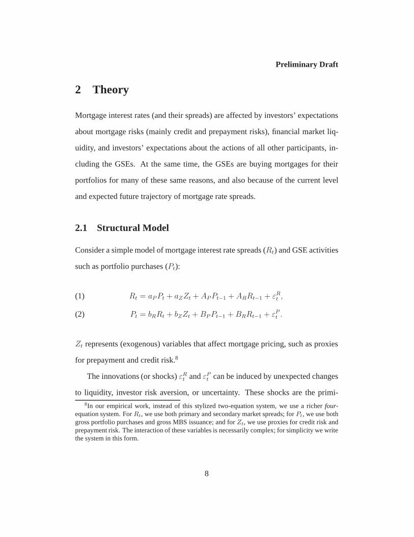
2 Theory

Mortgage interest rates (and their spreads) are affected by investors’ expectations

about mortgage risks (mainly credit and prepayment risks), financial market liq-

uidity, and investors’ expectations about the actions of all other participants, in-

cluding the GSEs. At the same time, the GSEs are buying mortgages for their

portfolios for many of these same reasons, and also because of the current level

and expected future trajectory of mortgage rate spreads.

2.1 Structural Model

Consider a simple model of mortgage interest rate spreads (Rt) and GSE activities

such as portfolio purchases (Pt):

Rt = aP Pt + aZZt + AP Pt−1 + ARRt−1 + εRt ,(1)

Pt = bRRt + bZZt + BP Pt−1 + BRRt−1 + εPt .(2)

Zt represents (exogenous) variables that affect mortgage pricing, such as proxies

for prepayment and credit risk.8

The innovations (or shocks)εRt andεP

t can be induced by unexpected changes

to liquidity, investor risk aversion, or uncertainty. These shocks are the primi-8In our empirical work, instead of this stylized two-equation system, we use a richerfour-

equation system. ForRt, we use both primary and secondary market spreads; forPt, we use bothgross portfolio purchases and gross MBS issuance; and forZt, we use proxies for credit risk andprepayment risk. The interaction of these variables is necessarily complex; for simplicity we writethe system in this form.

8

Preliminary Draft

tive exogenous forces which “buffet the system and cause oscillations” [Bernanke

(1986)]. In our empirical results we discuss the dynamic effects onR andP of

one standard deviation movements in these shocks.

Equations (1)–(2) provide a simple statistical description of the equilibrium

interaction of GSE actions, prices, and other observed and unobserved market

forces. The theoretical connection among these variables could be quite compli-

cated, in part because the equilibrium probably depends on how a small number of

entities expect the others to behave. Equation (1) captures the stabilizing effects

(if any) of GSE actions on spreads. Equation (2) captures the business decision

of the GSEs; in particular, how their portfolio managers react to movements in

spreads.

In this representation,aP is the contemporaneous effect of this period’s pur-

chases on this period’s spreads andAP is the direct effect of last period’s purchas-

es on this period’s spreads.9 In the same way,bR captures the contemporaneous

effect of spreads on purchases andBP captures the lagged direct effect.

Any model in which GSE purchases pushed down mortgage spreads in the

same period would imply thataP < 0. In the same way, any model in which wider

spreads increased GSE purchases in the same period would imply thatbR > 0.

These are only the very short-run effects, though. The long-run effect of GSE

purchases on spreads is the sum of the contemporaneous direct effect (aP ) and the

lagged direct effect (AP ); in addition, GSE purchases will affect spreads through9For clarity, we have here excluded more than one lagged value from our equations, although

in the empirical work we allow for an arbitrary number of lags. As we discuss in section 4.1, weuse two lags of the endogenous variables and one lag of the exogenous variables.

9

Preliminary Draft

the indirect effects of equation (2). Because these direct and indirect effects can

quickly become complicated, the standard method of describing them is via im-

pulse response functions. This is just the dynamic response of each of the vari-

ables in the system to a standard shock to eitherεPt (to capture the effect of an

unexpected increase in purchases) orεRt (to capture the effect of an unexpected

increase in spreads).

Granger causality tests and other statistical techniques examine the effects of

lagged variables on current variables, that is, whetherAP = 0 or BR = 0. Based

on these tests and our sensitivity analysis, as we discuss below, we conclude that

the statistical evidence supports the view that GSE actions react to interest rate

movements rather than the other way around.

2.2 Reduced-Form Estimates

Without additional assumptions, we cannot uniquely identifyboth the contempo-

raneous effect of purchases on spreads,aP , and the contemporaneous effect of

spreads on purchases,bR. To estimatebR we must restrictaP , either by forcing it

to be zero or by setting it to some value suggested by other data or theory. In the

same way, to estimateaP we must restrictbR.

In this simplified system, the identification problem can be seen by rewriting

the system of equations (1)–(2) with the contemporaneous terms on the left-hand

10

Preliminary Draft

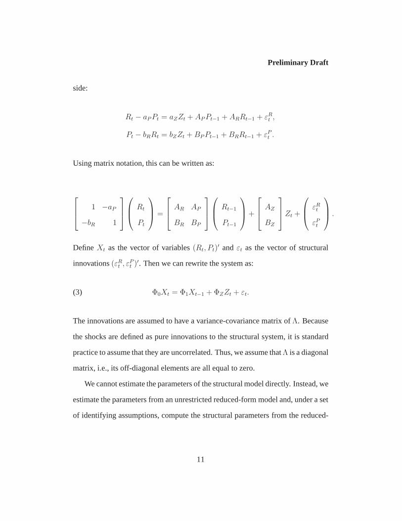
side:

Rt − aP Pt = aZZt + AP Pt−1 + ARRt−1 + εRt ,

Pt − bRRt = bZZt + BP Pt−1 + BRRt−1 + εPt .

Using matrix notation, this can be written as:

1 −aP

−bR 1

Rt

Pt

=

AR AP

BR BP

Rt−1

Pt−1

+

AZ

BZ

Zt +

εR

t

εPt

.

DefineXt as the vector of variables(Rt, Pt)′ and εt as the vector of structural

innovations(εRt , εP

t )′. Then we can rewrite the system as:

Φ0Xt = Φ1Xt−1 + ΦZZt + εt.(3)

The innovations are assumed to have a variance-covariance matrix ofΛ. Because

the shocks are defined as pure innovations to the structural system, it is standard

practice to assume that they are uncorrelated. Thus, we assume thatΛ is a diagonal

matrix, i.e., its off-diagonal elements are all equal to zero.

We cannot estimate the parameters of the structural model directly. Instead, we

estimate the parameters from an unrestricted reduced-form model and, under a set

of identifying assumptions, compute the structural parameters from the reduced-

11

Preliminary Draft

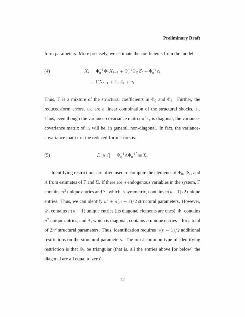
form parameters. More precisely, we estimate the coefficients from the model:

Xt = Φ−10 Φ1Xt−1 + Φ−1

0 ΦZZt + Φ−10 εt(4)

≡ ΓXt−1 + ΓZZt + ut.

Thus, Γ is a mixture of the structural coefficients inΦ0 and Φ1. Further, the

reduced-form errors,ut, are a linear combination of the structural shocks,εt.

Thus, even though the variance-covariance matrix ofεt is diagonal, the variance-

covariance matrix ofut will be, in general, non-diagonal. In fact, the variance-

covariance matrix of the reduced-form errors is:

E [uu′] = Φ−10 ΛΦ−1

0′ ≡ Σ.(5)

Identifying restrictions are often used to compute the elements ofΦ0, Φ1, and

Λ from estimates ofΓ andΣ. If there aren endogenous variables in the system,Γ

containsn2 unique entries andΣ, which is symmetric, containsn(n+1)/2 unique

entries. Thus, we can identifyn2 + n(n + 1)/2 structural parameters. However,

Φ0 containsn(n − 1) unique entries (its diagonal elements are ones),Φ1 contains

n2 unique entries, andΛ, which is diagonal, containsn unique entries—for a total

of 2n2 structural parameters. Thus, identification requiresn(n − 1)/2 additional

restrictions on the structural parameters. The most common type of identifying

restriction is thatΦ0 be triangular (that is, all the entries above [or below] the

diagonal are all equal to zero).

12

Preliminary Draft

Assuming thatΦ0 is triangular is tantamount to assumingeither that bR = 0

or thataP = 0. Under the assumption thataP = 0, contemporaneous shocks to

purchases,εPt , do not affect spreads,Rt, in periodt. However, contemporaneous

shocks to spreads,εRt , may affect purchases,Pt, in periodt.10 In other words,

under this assumption, GSE actions may respond to all information in a given

period, but spreads respond with a slight lag.

Under the alternative assumption thatbR = 0, contemporaneous shocks to

spreads,εRt , do not affect purchases,Pt, in periodt. However, contemporaneous

shocks to purchases,εPt , may affect spreads,Rt, in periodt. In other words, under

this assumption, spreads may react to all contemporaneous information while GSE

activities react with a slight lag.

The latter identifying assumption is consistent with the notion that spreads are

determined continuously over time in financial markets, while GSE activities are

the result of slower-moving business decisions. However, we also consider several

different identifying assumptions as robustness checks on our preferred, baseline

specification.

3 Data

We obtained consistent data on GSE portfolio purchases, securitization volume,

and mortgage interest rate spreads at a monthly frequency for the ten-year period

1994–2003, for 120 total observations. In addition, our dataset contains covariates10Because no restrictions are placed onΦ1, shocks to either purchases or spreads in periodt can

affect both purchases and spreads in periodt + 1.

13

Preliminary Draft

designed to control for credit and prepayment risk.

Our measure of GSE portfolio purchases is the sum of Fannie Mae and Fred-

die Mac’s gross retained portfolio purchases of mortgage assets, including whole

loans, own MBS, and other MBS.11 Our measure of securitization volume is the

sum of Fannie Mae and Freddie Mac’s gross issuance of MBS. These data are

available on the GSEs’ monthly summary reports.

As part of our robustness analysis, we normalize portfolio purchases and gross

MBS issuance by measures of the size of the residential mortgage market. We fol-

low other studies in using the monthly total volume ofnewresidential mortgages

originated (both purchase and refinance) as our measure of total market size. We

estimate this measure with the time series of mortgage originations as reported

under the Home Mortgage Disclosure Act (HMDA).

We use both primary and secondary market interest rates to compute our mea-

sures of mortgage rate spreads. The primary market mortgage rate is defined as

the monthly average interest rate on new 30-year fixed-rate mortgages, from Fred-

die Mac’s primary mortgage market survey. Secondary market mortgage rates are

defined as the monthly average current coupons on Fannie Mae and Freddie Mac

30-year MBS.12

We do not use the levels of these primary and secondary market mortgage rates

in our analysis; instead, as is common practice, we use the spread to a relevant11Measuring the effects of GSE portfolio purchases is difficult because there can be long lags

between when a GSE commits to a mortgage purchase and when the purchase is brought onto theGSEs’ books. However, the GSEs do not release enough data publicly to attempt to adjust forthese lags.

12The use of month-end data did not materially alter our results.

14

Preliminary Draft

risk-free rate. We have experimented with a variety of different measures of the

risk-free rate. However, in our analysis here we report results using the spreads to

a simple average of the 5-year and 10-year Treasury rates. Our results are almost

completely unchanged by the choice of interest rate index. As shown in table

1, changes in GSE debt yields, Treasury yields, and swap yields are very highly

correlated.13

The primary risks priced into mortgage rates (but not risk-free rates) are credit

risk (the risk of default) and prepayment risk (the risk of refinancing). As a proxy

for credit risk, we use the realized serious delinquency rate on conforming mort-

gages owned by the GSEs.14 We proxy prepayment risk with a measure of the

incentive to refinance. In particular, we use the mortgage coupon gap—the spread

between the weighted average coupon on existing securitized 30-year mortgages

and the 30-year fixed-rate mortgage rate.

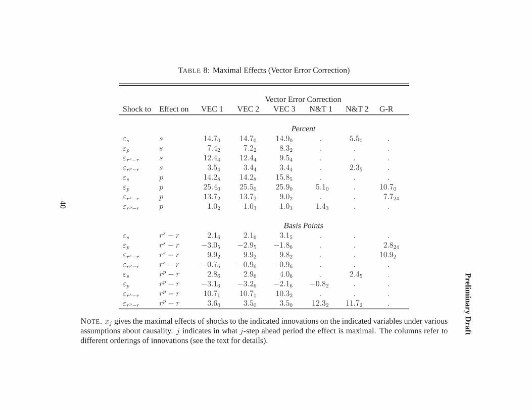
Descriptive statistics for key series are provided in table 2. Figure 1 plots

the time series of GSE portfolio purchases, GSE securitization volume, mortgage

market spreads, and mortgage delinquencies and the coupon gap. Note that the

financial market crisis of October 1998 was associated with a sharp widening

of spreads; as shown in the figure, primary market spreads rose about 70 basis

points. Serious mortgage delinquencies have a fairly narrow range, between 45

and 62 basis points; the coupon gap has varied substantially from−102 to +168

basis points.13We also used a simple average of 5-year and 10-year swaps and found no significant differ-

ences in our results.14“Serious delinquencies” are defined as mortgages 90 or more days past due or in foreclosure.

15

Preliminary Draft

4 VAR Results

In this section we examine the relationship between GSE activities and mortgage

market spreads using VAR techniques. We compute the dynamic responses of

mortgage rate spreads to an unexpected shock to GSE activities under our base-

line identifying assumption. Our primary specification is in first-differences; we

also report a full set of results under an alternative specification in normalized lev-

els. As a robustness check on these results, we examine the cumulative impulse

responses under a variety of alternative identifying assumptions. We also show

that GSE actions during the liquidity crisis of 1998 were not extraordinary; fur-

ther, had GSEs done nothing during this period, primary and secondary market

spreads would have evolved in about the same way.

4.1 Estimation

We estimate the parameters of an unrestricted reduced-form VAR as described in

section 2.2. Rather than use the levels of the variables, we estimated the model

using first-differences of the variables. (We use the logs of portfolio purchases

and securitization activity.) As shown in table 3 we find evidence that some of the

variables might have unit roots in their levels; however, each series is stationary

in first differences.15

We determined the optimal number of lags to include in our specification using15We have also estimated this VAR under a wide variety of alternative variable definitions,

including a specification with thelevel of spreads and thegrowth of GSE activity. Our resultswere in line with those reported here: GSE actions, especially portfolio purchases, have very littleeffect on spreads.

16

Preliminary Draft

the Akaike Information Criterion (AIC). We found that 2 lags of the endogenous

variables (GSE actions and spreads) and 1 lag of the exogenous variables (prepay-

ment and credit risk proxies) minimized the criterion.

We are interested in testing the ability of GSEs to stabilize mortgage markets

as well as to lower mortgage spreads in the long run. However, these two goals are

not necessarily equivalent. The GSEs might be able to dramatically affect spreads

in the short run, but then see these effects undone over time, leaving spreads un-

changed in the long run. Conversely, the GSEs might be unable to affect spreads

very much in a given month, but might be able to cumulate their effects over time,

producing a significant long-run effect without large effects in any given period.

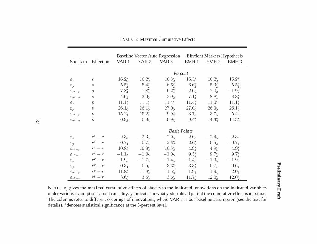
For our baseline model, we report a full set of impulse response functions.

For the alternative specifications and identifying assumptions, we summarize the

short- and long-run effects of GSEs on rates with two statistics: The cumulative

impulse response after 24 months and the largest cumulative effect (and when that

effect occurs).

4.2 Results Under Baseline Identification

We impose a triangular (Wold) representation on our system of equations to ex-

amine the impulse response functions. (See section 2 for a discussion of this

procedure.) This requiresassumingthat certain variables in our system do not

respond contemporaneously to shocks in other equations. However, we do not re-

strict any of the lagged effects, so all endogenous variables may react to any shock

in the previous period. (As we discussed, we do not estimate reaction functions

17

Preliminary Draft

for credit and prepayment risk, but rather take these two variables as exogenous

to our system.)

In our baseline identification, we assume that shocks to GSE activities have no

contemporaneous effect on mortgage market spreads. That is, we assume that the

ordering of innovations in the Cholesky decomposition is: [εrs−r, εrp−r, εs, εp].

Later, we compute impulse response functions under several alternatives to this

baseline assumption.

Intuitively, our ordering of contemporaneous responses assumes that the GSEs

observe all available information in a period before reacting. Our ordering thus

perforce assumes that shocks to secondary market spreads occur during a period

and are not affected by GSE actions during the rest of the period. Primary market

spreads react to secondary market spreads, but not to GSE actions. Of the GSE

actions, gross MBS issuance reacts to spreads, and portfolio purchase volume

reacts to all contemporaneous variables.

We consider several alternatives to our baseline ordering, including several

in which spreads react to GSE actions. Under these alternatives, though, GSE

actions have less of a long-run effect on mortgage rate spreads.

With an assumption about the contemporaneous effects of shocks in our sys-

tem, we can estimate the effect of orthogonalized one standard deviation shocks

of each innovation on each of our endogenous variables. In other words, we can

estimate, for example, the dynamic response of primary mortgage market spreads

to a one-time standardized shock to the portfolio purchase equation. A complete

set of these impulse response functions is shown in figure 2. Each panel shows the

18

Preliminary Draft

effects of one standard deviation shocks of each innovation on a given variable.

Effect of Shock to Secondary Market Spreads (εrs−r) Cumulating the effects

across all months, a one standard deviation shock to the secondary market spread

innovation (about 8 basis points) ultimately leads to a 9.9 basis point increase in

the secondary market spread, an 11 basis point increase in the primary market

spread, a 7.3 percent increase in securitization, and a 14.1 percent increase in pur-

chases. The largest cumulative effects have occurred within three or four months

of the shock.

Effect of Shock to Primary Market Spreads (εrp−r) In the same way, a one

standard deviation shock to the primary market spread innovation (about 4 basis

points) ultimately leads to a 2.5 basis point increase in the primary market spread,

a 1.1 basis point decrease in the secondary market spread, a 3.9 percent increase

in securitization, and a 0.2 percent increase in purchases. Here, the largest cumu-

lative effects take up to five months to occur.

Effect of Shock to GSE Actions (εs and εp) Turning to the effects of shocks to

the securitization and portfolio innovations, we find that a one standard deviation

shock to the securitization innovation (about 16 percent) ultimately leads to a 14.6

percent increase in securitization, an 8.7 percent increase in purchases, a 2.1 basis

point decline in the secondary market spread, and a 1.7 basis point decline in the

primary market spread—with the largest cumulative effects occurring within five

months of the shock.

19

Preliminary Draft

A one standard deviation shock to the portfolio purchase innovation (about

26 percent) ultimately leads to a 17 percent increase in purchases, a 3.8 percent

increase in securitization, a 0.5 basis point decline in the secondary market spread,

and a 0.2 basis point decline in the primary market spread.16 Here, the largest

cumulative effects have taken place within four months of the shock.

Thus, based on our impulse response analysis, we estimate that if the GSEs

unexpectedly increase their portfolio purchases by $10 billion (or 12.7 percent

of the 2003 average), the secondary market spread would decline about 0.3 basis

points and the primary market spread would decline about 0.1 basis points over

the long-run. But if the GSEs instead unexpectedly increased their securitization

activity by $10 billion (or 6.3 percent of the 2003 average), we estimate that the

secondary market spread would decline about 0.8 basis points and the primary

market spread would decline about 0.7 basis points. These results suggest that

GSE portfolio purchases have economically and statistically negligible effects on

mortgage market spreads, even in the long run. Further, portfolio purchases are not

more effective at reducing mortgage market spreads than securitization activities.

Variance Decomposition Figure 3 shows variance decomposition proportions

for the key data series. Variance decompositions indicate how much of the forecast

error in a series is due to a shock to its own innovation and how much is due to

shocks to other innovations. As shown, GSE activities account for very little of the16The average (absolute) month-to-month change in GSE portfolio purchases is 24 percent.

Moreover, such a shock amounts to less than 0.6 percent of the GSEs’ combined retained portfo-lios.

20

Preliminary Draft

forecast errors of mortgage market spreads. Secondary market spreads, however,

account for a sizable proportion of the forecast errors of primary market spreads

and portfolio purchase volume.

4.3 The 1998 Liquidity Crisis

In a dramatic example of the dynamics of the system, from August 1998 to Oc-

tober 1998, secondary market spreads widened about 69 basis points as a result

of a liquidity shock. During the same time, primary market spreads widened 78

basis points, securitization volume decreased 5 percent, and portfolio purchases

jumped 76 percent.

Obviously, during this period, spreads and purchases moved much more than

during normal periods. As a test of our model’s ability to explain GSE behavior

and the evolution of spreads, we initialized the model with the secondary market

spread changes in September and October and allowed the system to evolve en-

dogenously without any other information. As shown by the first panel of figure 4,

we forced secondary market spreads to increase about 30 basis points in Septem-

ber and 39 basis points in October. We then allowed secondary market spreads to

evolve as predicted by the model. As shown, the model predicted that the changes

in spreads would gradually decline to zero. In reality, spreads jumped around our

model’s prediction in reaction to incoming data (such as prepayment and credit

risk information). Primary market spreads, the next panel, show about the same

dynamics.

Turning to GSE actions, the next two panels show that our model is success-

21

Preliminary Draft

ful in predicting purchase volume in the peak crisis period, September through

December 1998. Our model cannot explain the big drop in purchases in January

1999, or the offsetting rise in February 1999. However, in the long run these fore-

cast errors roughly cancel out, leaving the predicted net change in purchases over

the entire period close to the actual change. Our model also does a decent job of

predicting securitization volume through this episode. Actual MBS issuance was

much more volatile than predicted by our model, although, again, the forecast

errors net out to about zero.

Thus, the GSEs’ portfolio purchases during this period of financial market

stress can be explained almost completely by their historical pattern of buying

mortgages when spreads are wide. That is, there was nothing special about the

GSEs’ actions during this period of financial market stress.

However, even though GSE actions during the crisis were roughly consistent

with their behavior at other times, it could be that the magnitudes in this particular

episode were large enough to mitigate the effects on spreads. To test this theo-

ry, we computed the changes in spreads that would have occurred had the GSEs

not changed their portfolio behavior during the crisis. In other words, we force

portfolio purchases to be constant at $30.5 billion through the episode.

In figure 4, the difference between this counterfactual experiment (the dotted

line) and the model’s prediction (the dashed line) is our estimate of the effect

of GSE portfolio purchases on the mortgage market during the crisis period. As

shown, the GSEs’ portfolio purchases appear to have had little effect on either

primary or secondary mortgage market spreads. However, there was a substantial

22

Preliminary Draft

effect on securitization activity.

4.4 Results Under Alternative Identifying Assumptions

With four endogenous variables in our system there are potentially four factori-

al, or 24, different triangular representations of the system. The previous section

reported results in detail under our baseline identification assumptions. In this

section, we summarize results under several alternative representations. We focus

on two classes of alternatives: first, reasonable reorderings of our baseline specifi-

cation (VAR) and, second, orderings suggested by the efficient markets hypothesis

(EMH).

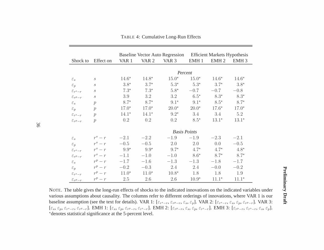
For each alternative ordering, we summarize the long-run response of vari-

ables to shocks with the cumulative impulse response functions shown in table 4.

We also summarize the short-run response of variables to shocks by reporting the

largest cumulative response in table 5. The column labeled VAR 1 in the table

reports the results under our baseline specification, which we have already dis-

cussed. From a policy perspective, the most interesting results are the effects of

GSE actions on mortgage market spreads. As shown, these effects are negligible

and do not vary significantly under the different identifying assumptions.

4.4.1 Reorderings of Baseline Specification

It could be argued that spreads react to all information available in a given month,

while GSE actions are somewhat constrained by prior agreements with origina-

tors. In other words, mortgage spreads react continuously to information flow,

23

Preliminary Draft

while portfolio purchases and MBS issuance have more inertia.

The alternative representations, labeled VAR 2 and VAR 3, assume some de-

gree of inertia in GSE actions. In VAR 2, the primary market spread reacts con-

temporaneously to shocks to GSE actions and the secondary market spread. GSE

actions, in turn, react contemporaneously only to shocks to the secondary market

spread. In VAR 3, primary and secondary market spreads react contemporaneous-

ly to shocks to GSE actions. GSE actions, in turn, do not react contemporaneously

to shocks to spreads.

The first three columns of tables 4–5 summarize the results under the baseline

and alternative orderings. As shown, the results are not very different under the

alternatives than under the baseline ordering. In particular, shocks to GSE actions

continue to have small effects on mortgage market spreads.

4.4.2 Efficient Markets Hypothesis

The efficient markets hypothesis (EMH) maintains that an asset’s price ought to

reflect all relevant available information about that asset. The EMH can have

strong implications for identification in VARs (see Sarno and Thornton, 2004).

Our system contains two endogenous asset price variables: the secondary market

spread and the primary market spread. Under a triangular representation, these

two variables cannot react to the same set of shocks, so we must order them

by their relative inertia. Primary mortgage market interest rates (and thus their

spreads) are relatively sticky for the reasons discussed earlier. In addition, our

measure of the primary market rate is Freddie Mac’s survey of lenders, which is

24

Preliminary Draft

conducted only weekly.

In table 4, the column labeled EMH 1 reports results under a strong version

of the EMH: GSE actions do not respond to shocks to any asset price equations.

The columns labeled EMH 2 and EMH 3 report results under slightly relaxed ver-

sions of the EMH. In EMH 2, GSE actions respond to primary market shocks.

In EMH 3, GSE actions react to both primary and secondary market shocks. As

shown in the tables, these alternative orderings do not significantly alter our base-

line results.

4.5 Results Under a Levels Specification

The results reported in section 4.2 were based on a model estimated using the

first-difference of mortgage spreads and the percent changes in GSE activity. We

adopted this as our primary specification because GSE activity is clearly non-

stationary and GSE spreads, while probably stationary, are highly persistent. An-

other approach is to normalize GSE actions by some measure of the size of the

market and estimate the model using normalized GSE actions and the level of

spreads. Note that both spreads and normalized GSE actions are fairly persistent,

so these results may be contaminated by a common trend in both sets of variables.

As we discussed in section 3, we normalize GSE portfolio purchases and gross

MBS issuance by estimates of mortgage originations derived from the HMDA

reports. The normalized time series are shown in figure 5.

We follow the same estimation procedure as before. For completeness, we

report a full set of impulse response functions in figure 6. Note the extreme per-

25

Preliminary Draft

sistence of shocks. In many cases the shocks continue to affect variables five

years after the initial period. The top two panels of the figure show the response

of spreads to standardized shocks to other variables, including GSE actions. As

before, shocks to portfolio purchases have no statistically significant effect on

mortgage rate spreads. Thus, our main results are unchanged.

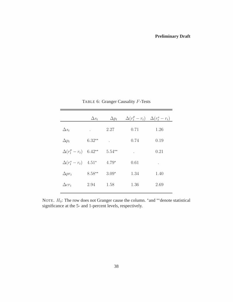
4.6 Granger Causality Results

F -test statistics from bivariate Granger causality tests among all variables in the

system are reported in table 6. The null hypothesis in these tests is that the vari-

able in the table row does not Granger-cause the variable in the table column.

For convenience, if we can reject the null we say that the row Granger-causes the

column (as opposed to saying that the row does not “not Granger cause” the col-

umn). From table 6 we see that mortgage market spreads Granger-cause portfolio

purchases and securitization volume, but not the converse. Also note that securi-

tization volume and portfolio purchases Granger-cause each other. These results

are summarized in figure 7.

5 Cointegration Analysis

Other studies, most notably Naranjo and Toevs (2002), have used cointegration

techniques to study the statistical relationship between GSE actions and mortgage

market spreads. In effect, these techniques require the assumption that all vari-

ables in the system contain a common trend. This assumption is reasonable for

26

Preliminary Draft

variables such as the level of gross MBS issuance and the level of portfolio pur-

chases. However, this assumption is economically less reasonable for variables

such as mortgage rate spreads and the relative level of GSE actions. Nonetheless,

we proceed with the cointegration analysis for comparison with earlier studies.

In this section we once again examine the impulse responses of variables in

the system under the assumption that all variables are cointegrated. In place of our

VAR, we estimate the parameters from a vector error-correction model, or VECM.

As in the VAR analysis, we use a standard set of identifying restrictions.

There are several economic and statistical reasons to doubt the estimates pro-

duced under this specification. First, the estimated cointegrating relationship is

primarily between securitization and portfolio purchases; mortgage market spreads,

the key variables of policy concern, are statistically insignificant elements of coin-

tegrating vector. Second, it is statistically difficult to distinguish between unit root

and near unit root series, so it is possible that the estimated long-run relationship

is spurious.17 Third, we cannot establish that each of our endogenous variables

is integrated of the same order. Last, it is generally accepted that interest-rate

spreads cannot in principle be integrated of order one. That we cannot statistical-

ly reject this hypothesis is the result of using cointegration techniques over short

time spans. We therefore discount the results in this section and emphasize our

VAR results in section 4.17If the system is trulynot cointegrated, using cointegration techniques can produce spurious

results. If the system is truly cointegrated, however, using a difference-stationary VAR producescorrect, albeit possibly inefficient, results.

27

Preliminary Draft

5.1 VECM Results

For the system defined in equation (3) to be cointegrated, a necessary condition

is that each component ofXt be integrated of the same order (for example, each

component ofXt has a unit root and is stationary in first differences). Additional-

ly, there must be at least one linear combination ofXt that is stationary. As shown

in table 3, portfolio purchases might not contain a unit root. This is similar to the

result reported by Gonzalez-Rivera (2001).

To examine the second necessary condition for cointegration, we use Johansen’s

(1988, 1991) maximum likelihood procedures to estimate any long-run cointegrat-

ing relationships in equation 3. Johansen’s trace and max statistics suggest that

our system of equations has multiple cointegrating relationships. The first rela-

tionship can be written as:

(6) ε̂t = 1.1882 + 0.0188(rpt − rt) − 0.0050(rs

t − rt) − 1.8534st + pt.

Here, ε̂t denotes the deviations from the estimated long-run relationship. Note

that we have normalized with respect to GSE portfolio purchases, sopt has a unit

coefficient in this representation.

Figure 8 shows actual purchases, the equilibrium level of purchases (that is,

the level consistent with the long-run relation given the actual values for other

variables in equation 6), and the deviations from the long-run path. Purchases

do track their long-run levels, but the deviations are frequent and exhibit serial

correlation for extended periods, reaffirming the potential problems with using

28

Preliminary Draft

cointegration techniques in such a setting.

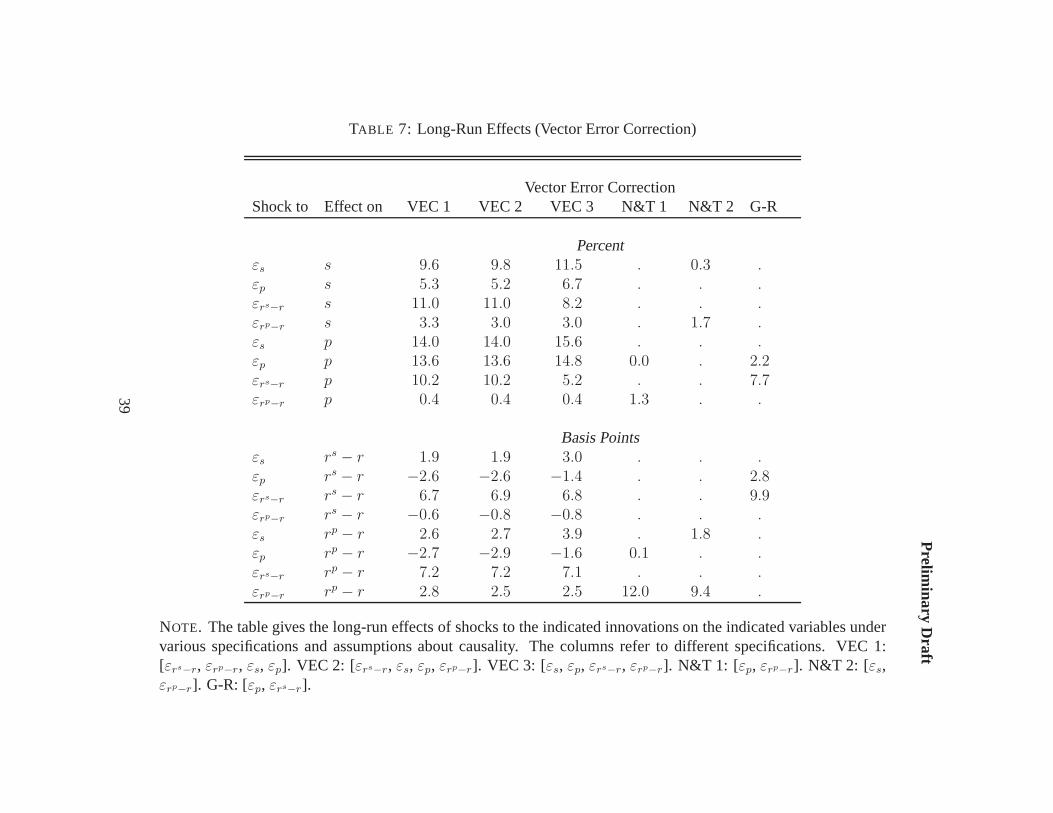
Tables 7–8 summarize the impulse responses for each endogenous variable to

shocks to each structural innovation for three different orderings of innovations.

The results, once again, are similar to those from our baseline VAR specification:

GSE portfolio purchases have negligible effects on mortgage market spreads.

5.2 Comparison With Other Studies

For comparability, we also estimate the Naranjo and Toevs (2002) and Gonzalez-

Rivera (2001) specifications using our dataset. We find that under Naranjo and To-

evs’s specification, unanticipated shocks to GSE portfolio purchases again have no

meaningful effect on mortgage market spreads. Under Gonzalez-Rivera’s specifi-

cation, unanticipated shocks to GSE portfolio purchases increase secondary mar-

ket mortgage spreads slightly. However, as we discussed, these results are ob-

tained under strong and unrealistic assumptions.

Moreover, Naranjo and Toevs normalize portfolio purchases and securitization

by the size of the mortgage market to relate GSE activity to the primary mortgage

spread. We use an estimate of mortgage originations derived from HMDA data as

the normalization. As shown in tables 7–8, an unanticipated increase in the GSEs’

portfolio purchase share of the market of about 5 percent has little effect on the pri-

mary market spread. Conversely, an unanticipated increase in the primary market

spread of about 9 basis points leads to an increase in the GSE portfolio purchase

share of the market of slightly over 1 percent. Similarly, an unanticipated 5.5 per-

cent increase in the GSEs securitization share of mortgage originations leads to

29

Preliminary Draft

1.8 basis point increase in the primary market spread, and an unanticipated 9 ba-

sis point increase in the primary market spread increases the GSEs’ securitization

share of mortgage originations nearly 2 percent. Note that under this specification,

we can find no evidence that GSE activities decrease mortgage market spreads or

that portfolio purchases are in any sense better than securitization activity.

Gonzalez-Rivera (2001) relates the raw level of (net) portfolio purchases to the

secondary market spread. Under this specification, an unexpected increase in GSE

portfolio purchases of $11 billion decreases the secondary market spread nearly

3 basis points. An unexpected 8 basis point increase in the secondary mortgage

market spread increases GSE portfolio purchases nearly $8 billion.

6 Conclusion

This paper examines the statistical evidence of a connection between GSE sec-

ondary market actions and the interest rates paid by mortgage borrowers. While

GSE portfolio purchases benefit GSE shareholders directly, the purchases must

lower the mortgage rate paid by the homeowner in order to have a wider social

benefit.

We find, however, that portfolio purchases has economically and statistically

negligible effects on mortgage rates. Further, portfolio purchases are not any more

effective at decreasing spreads than securitization volume. Our results were robust

to several alternative identifying assumptions, including those suggested by the

efficient markets hypothesis.

30

Preliminary Draft

Earlier studies by Naranjo and Toevs (2002) and Gonzalez-Rivera (2001) found

that GSE actions did significantly affect mortgage spreads. We repeated the coin-

tegration analyses used in those studies with our more recent data set and found,

again, that GSE actions have only negligible effects on mortgage spreads.

Further, we studied the 1998 liquidity crisis and found that GSE actions gener-

ally followed the predictions of the model. Had GSE actions remained unchanged

through this episode, we estimate that mortgage spreads paid by borrowers would

have been essentially unchanged. Thus, the GSEs do not appear to have played a

significant role in managing mortgage market risks through the 1998 crisis.

References

Ambrose, B., M. LaCour-Little, and A. Sanders (2004). The effect of con-forming loan status on mortgage yield spreads: A loan level analysis.RealEstate Economics 32, 541–69.

Bernanke, B. S. (1986). Alternative explanations of the money-income corre-lation.Carnegie-Rochester Conference Series on Public Policy 25, 49–99.

Gonzalez-Rivera, G. (2001). Linkages between secondary and primary marketsfor mortgages.Journal of Fixed Income 11, 29–36.

Hancock, D., A. Lehnert, W. Passmore, and S. Sherlund (Forthcoming). BaselII capital standards: Potential impacts on mortgage rates and securitizationmarkets. Manuscript, Federal Reserve Board, Washington DC.

Johansen, S. (1988). Statistical analysis of cointegration vectors.Journal ofEconomic Dynamics and Control 12, 231–54.

Johansen, S. (1991). Estimation and hypothesis testing of cointegration vectorsin Gaussian vector autoregressive models.Econometrica 59, 1551–80.

Johansen, S. and K. Juselius (1992). Testing structural hypotheses in a multi-variate cointegration analysis of the PPP and the UIP for the UK.Journal

31

Preliminary Draft

of Econometrics 53, 211–44.

McKenzie, J. (2002). A reconsideration of the jumbo/non-jumbo mortgage ratedifferential.Journal of Real Estate Finance and Economics 25, 197–214.

Naranjo, A. and A. Toevs (2002). The effects of purchases of mortgagesand securitization by government sponsored enterprises on mortgage yieldspreads and volatility.Journal of Real Estate Finance and Economics 25,173–96.

Passmore, W., S. Sherlund, and G. Burgess (2004). The effect of housinggovernment-sponsored enterprises on mortgage rates. Forthcoming.

Sarno, L. and D. L. Thornton (2004). The efficient market hypothesis and iden-tification in structural VARs.Federal Reserve Bank of St. Louis Review 86,49–60.

32

Preliminary Draft

TABLE 1: Correlations Among Interest Rates

10-year GSE Debt Treasury Swaps

GSE Debt 1.0000Treasury 0.9557 1.0000Swaps 0.9915 0.9688 1.0000

5-year GSE Debt Treasury Swaps

GSE Debt 1.0000Treasury 0.9720 1.0000Swaps 0.9960 0.9756 1.0000

NOTE. Table gives correlation coefficients amongmonthly differences in yieldson comparable debt instruments. Data are monthly averages, Jan. 2000 throughDec. 2003.

33

Prelim

inaryD

raft

TABLE 2: Descriptive Statistics

Variable Symbol Mean Median Std. Dev. Min Max

Securitization Volume ($bn) st 54.70 35.11 47.70 7.47 204.28Portfolio Purchase Volume ($bn) pt 28.44 19.84 26.82 3.45 148.67Primary Market Spread (bps) rp

t − rt 181.05 173.69 39.20 122.95 268.52Secondary Market Spread (bps) rs

t − rt 144.81 143.70 28.21 102.68 203.56Mortgage Coupon Gap (bps) prt 45.12 55.92 61.26 −101.92 168.45Mortgage Delinquencies (bps) crt 53.27 54.00 5.10 45.00 62.00

NOTE. Statistics are for 120 monthly observations running from January 1994 through December 2003.

34

Prelim

inaryD

raft

TABLE 3: Augmented Dickey-Fuller Unit Root Tests

Levels First DifferencesVariable Intercept Intercept+Trend Intercept Intercept+Trend

Securitization Volume st −1.12 −3.21 −4.70?? −4.61??

Portfolio Purchase Volume pt −1.60 −3.52? −7.00?? −6.96??

Primary Market Spread rpt − rt −1.67 −3.87? −5.75?? −5.72??

Secondary Market Spread rst − rt −2.22 −3.70? −6.37?? −6.35??

Mortgage Coupon Gap prt −2.67 −2.78 −5.75?? −5.68??

Mortgage Delinquencies crt −1.74 −1.73 −3.88?? −3.86??

NOTE. H0: Unit root. ?and??denote statistical significance at the 5- and 1-percent levels, respectively.

35

Prelim

inaryD

raftTABLE 4: Cumulative Long-Run Effects

Baseline Vector Auto Regression Efficient Markets HypothesisShock to Effect on VAR 1 VAR 2 VAR 3 EMH 1 EMH 2 EMH 3

Percentεs s 14.6? 14.8? 15.0? 15.0? 14.6? 14.6?

εp s 3.8? 3.7? 5.3? 5.3? 3.7? 3.8?

εrs−r s 7.3? 7.3? 5.8? −0.7 −0.7 −0.8εrp−r s 3.9 3.2 3.2 6.5? 8.3? 8.3?

εs p 8.7? 8.7? 9.1? 9.1? 8.5? 8.7?

εp p 17.0? 17.0? 20.0? 20.0? 17.6? 17.0?

εrs−r p 14.1? 14.1? 9.2? 3.4 3.4 5.2εrp−r p 0.2 0.2 0.2 8.5? 13.1? 13.1?

Basis Pointsεs rs − r −2.1 −2.2 −1.9 −1.9 −2.3 −2.1εp rs − r −0.5 −0.5 2.0 2.0 0.0 −0.5εrs−r rs − r 9.9? 9.9? 9.7? 4.7? 4.7? 4.8?

εrp−r rs − r −1.1 −1.0 −1.0 8.6? 8.7? 8.7?

εs rp − r −1.7 −1.6 −1.3 −1.3 −1.8 −1.7εp rp − r −0.2 −0.3 2.4 2.4 −0.0 −0.2εrs−r rp − r 11.0? 11.0? 10.8? 1.8 1.8 1.9εrp−r rp − r 2.5 2.6 2.6 10.9? 11.1? 11.1?

NOTE. The table gives the long-run effects of shocks to the indicated innovations on the indicated variables undervarious assumptions about causality. The columns refer to different orderings of innovations, where VAR 1 is ourbaseline assumption (see the text for details). VAR 1: [εrs−r, εrp−r, εs, εp]. VAR 2: [εrs−r, εs, εp, εrp−r]. VAR 3:[εs, εp, εrs−r, εrp−r]. EMH 1: [εs, εp, εrp−r, εrs−r]. EMH 2: [εrp−r, εs, εp, εrs−r]. EMH 3: [εrp−r, εrs−r, εs, εp].?denotes statistical significance at the 5-percent level.

36

Prelim

inaryD

raftTABLE 5: Maximal Cumulative Effects

Baseline Vector Auto Regression Efficient Markets HypothesisShock to Effect on VAR 1 VAR 2 VAR 3 EMH 1 EMH 2 EMH 3

Percentεs s 16.2?

0 16.2?0 16.3?

0 16.3?0 16.2?

0 16.2?0

εp s 5.5?2 5.4?

2 6.6?2 6.6?

2 5.3?2 5.5?

2

εrs−r s 7.8?4 7.8?

4 6.2?4 −2.02 −2.02 −1.92

εrp−r s 4.62 3.92 3.92 7.1?4 8.8?

4 8.8?4

εs p 11.1?1 11.1?

1 11.4?1 11.4?

1 11.0?1 11.1?

1

εp p 26.1?0 26.1?

0 27.0?0 27.0?

0 26.3?0 26.1?

0

εrs−r p 15.2?3 15.2?

3 9.9?2 3.75 3.75 5.45

εrp−r p 0.93 0.93 0.93 9.4?3 14.3?

3 14.3?3

Basis Pointsεs rs − r −2.35 −2.35 −2.05 −2.05 −2.45 −2.35

εp rs − r −0.74 −0.74 2.6?2 2.6?

2 0.52 −0.74

εrs−r rs − r 10.8?2 10.8?

2 10.5?2 4.9?

4 4.9?4 4.9?

4

εrp−r rs − r −1.15 −1.05 −1.05 9.5?2 9.7?

2 9.7?2

εs rp − r −1.95 −1.75 −1.45 −1.45 −1.95 −1.95

εp rp − r −0.34 0.51 3.3?1 3.3?

1 0.71 0.61

εrs−r rp − r 11.8?2 11.8?

2 11.5?3 1.94 1.94 2.04

εrp−r rp − r 3.6?0 3.6?

0 3.6?0 11.7?

2 12.0?2 12.0?

2

NOTE. xj gives the maximal cumulative effects of shocks to the indicated innovations on the indicated variablesunder various assumptions about causality.j indicates in whatj-step ahead period the cumulative effect is maximal.The columns refer to different orderings of innovations, where VAR 1 is our baseline assumption (see the text fordetails).?denotes statistical significance at the 5-percent level.

37

Preliminary Draft

TABLE 6: Granger CausalityF -Tests

∆st ∆pt ∆(rpt − rt) ∆(rs

t − rt)

∆st . 2.27 0.71 1.26

∆pt 6.32?? . 0.74 0.19

∆(rpt − rt) 6.42?? 5.54?? . 0.21

∆(rst − rt) 4.51? 4.79? 0.61 .

∆prt 8.58?? 3.09? 1.34 1.40

∆crt 2.94 1.58 1.36 2.69

NOTE. H0: The row does not Granger cause the column.?and??denote statisticalsignificance at the 5- and 1-percent levels, respectively.

38

Prelim

inaryD

raftTABLE 7: Long-Run Effects (Vector Error Correction)

Vector Error CorrectionShock to Effect on VEC 1 VEC 2 VEC 3 N&T 1 N&T 2 G-R

Percentεs s 9.6 9.8 11.5 . 0.3 .εp s 5.3 5.2 6.7 . . .εrs−r s 11.0 11.0 8.2 . . .εrp−r s 3.3 3.0 3.0 . 1.7 .εs p 14.0 14.0 15.6 . . .εp p 13.6 13.6 14.8 0.0 . 2.2εrs−r p 10.2 10.2 5.2 . . 7.7εrp−r p 0.4 0.4 0.4 1.3 . .

Basis Pointsεs rs − r 1.9 1.9 3.0 . . .εp rs − r −2.6 −2.6 −1.4 . . 2.8εrs−r rs − r 6.7 6.9 6.8 . . 9.9εrp−r rs − r −0.6 −0.8 −0.8 . . .εs rp − r 2.6 2.7 3.9 . 1.8 .εp rp − r −2.7 −2.9 −1.6 0.1 . .εrs−r rp − r 7.2 7.2 7.1 . . .εrp−r rp − r 2.8 2.5 2.5 12.0 9.4 .

NOTE. The table gives the long-run effects of shocks to the indicated innovations on the indicated variables undervarious specifications and assumptions about causality. The columns refer to different specifications. VEC 1:[εrs−r, εrp−r, εs, εp]. VEC 2: [εrs−r, εs, εp, εrp−r]. VEC 3: [εs, εp, εrs−r, εrp−r]. N&T 1: [εp, εrp−r]. N&T 2: [εs,εrp−r]. G-R: [εp, εrs−r].

39

Prelim

inaryD

raftTABLE 8: Maximal Effects (Vector Error Correction)

Vector Error CorrectionShock to Effect on VEC 1 VEC 2 VEC 3 N&T 1 N&T 2 G-R

Percentεs s 14.70 14.70 14.90 . 5.50 .εp s 7.42 7.22 8.32 . . .εrs−r s 12.44 12.44 9.54 . . .εrp−r s 3.54 3.44 3.44 . 2.35 .εs p 14.28 14.28 15.85 . . .εp p 25.40 25.50 25.90 5.10 . 10.70

εrs−r p 13.72 13.72 9.02 . . 7.724

εrp−r p 1.02 1.03 1.03 1.43 . .

Basis Pointsεs rs − r 2.16 2.16 3.15 . . .εp rs − r −3.05 −2.95 −1.86 . . 2.824

εrs−r rs − r 9.92 9.92 9.82 . . 10.92

εrp−r rs − r −0.76 −0.96 −0.96 . . .εs rp − r 2.86 2.96 4.06 . 2.45 .εp rp − r −3.16 −3.26 −2.16 −0.82 . .εrs−r rp − r 10.71 10.71 10.32 . . .εrp−r rp − r 3.60 3.50 3.50 12.32 11.72 .

NOTE. xj gives the maximal effects of shocks to the indicated innovations on the indicated variables under variousassumptions about causality.j indicates in whatj-step ahead period the effect is maximal. The columns refer todifferent orderings of innovations (see the text for details).

40

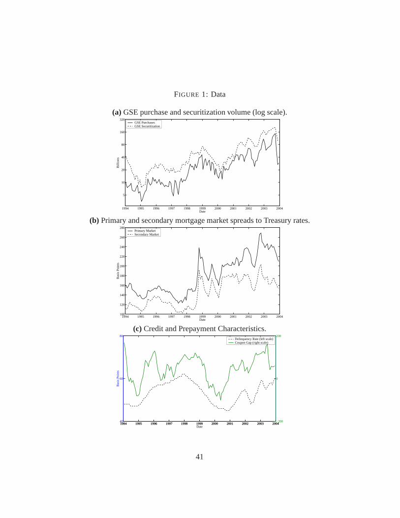
FIGURE 1: Data

(a) GSE purchase and securitization volume (log scale).

1994 1995 1996 1997 1998 1999 2000 2001 2002 2003 2004

5

10

20

40

80

160

320

Date

Bill

ions

GSE PurchasesGSE Securitization

(b) Primary and secondary mortgage market spreads to Treasury rates.

1994 1995 1996 1997 1998 1999 2000 2001 2002 2003 2004100

120

140

160

180

200

220

240

260

280

Date

Bas

is P

oint

s

Primary MarketSecondary Market

(c) Credit and Prepayment Characteristics.

1994 1995 1996 1997 1998 1999 2000 2001 2002 2003 200440

60

80

Date

Bas

is P

oint

s

Delinquency Rate (left scale)Coupon Gap (right scale)

1994 1995 1996 1997 1998 1999 2000 2001 2002 2003 2004−200

0

200

41

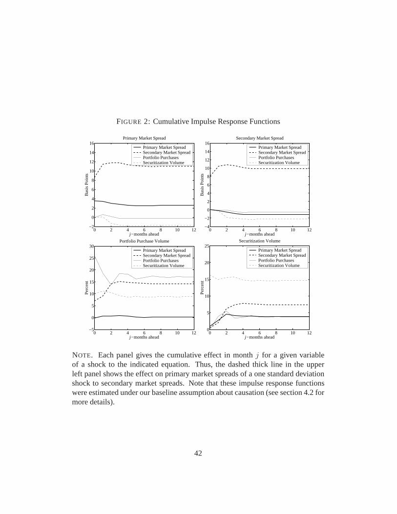
FIGURE 2: Cumulative Impulse Response Functions

0 2 4 6 8 10 12−2

0

2

4

6

8

10

12

14

16Primary Market Spread

j− months ahead

Bas

is P

oint

s

Primary Market SpreadSecondary Market SpreadPortfolio PurchasesSecuritization Volume

0 2 4 6 8 10 12−4

−2

0

2

4

6

8

10

12

14

16Secondary Market Spread

j− months ahead

Bas

is P

oint

s


0 2 4 6 8 10 12−5

0

5

10

15

20

25

30Portfolio Purchase Volume

j− months ahead

Per

cent


0 2 4 6 8 10 120

5

10

15

20

25Securitization Volume

j− months ahead

Per

cent


NOTE. Each panel gives the cumulative effect in monthj for a given variableof a shock to the indicated equation. Thus, the dashed thick line in the upperleft panel shows the effect on primary market spreads of a one standard deviationshock to secondary market spreads. Note that these impulse response functionswere estimated under our baseline assumption about causation (see section 4.2 formore details).

42

FIGURE 3: Variance Decomposition

0 5 10 15 20 250

20

40

60

80


j− months ahead

Per

cent Primary Market Spread

Secondary Market SpreadPortfolio PurchasesSecuritization Volume

0 5 10 15 20 250

20

40

60

80


j− months ahead

Per



0 5 10 15 20 250

20

40

60

80


j− months ahead

Per



0 5 10 15 20 250

20

40

60

80


j− months ahead

Per



NOTE. Each panel gives the fraction of thej−month ahead forecast error vari-ance for a given variable that can be explained by innovations to the indicatedequations.

43

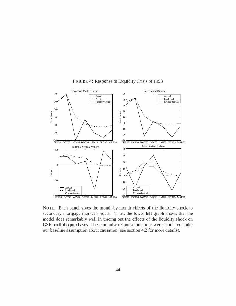
FIGURE 4: Response to Liquidity Crisis of 1998

SEP98 OCT98 NOV98 DEC98 JAN99 FEB99 MAR99−20

−10

0

10

20

30


Bas

is P

oint

s

ActualPredictedCounterfactual


−20

−10

0

10

20

30

40


Bas

is P

oint

s



−50

0


Per

cent



−20

−10

0

10

20

30


Per

cent


NOTE. Each panel gives the month-by-month effects of the liquidity shock tosecondary mortgage market spreads. Thus, the lower left graph shows that themodel does remarkably well in tracing out the effects of the liquidity shock onGSE portfolio purchases. These impulse response functions were estimated underour baseline assumption about causation (see section 4.2 for more details).

44

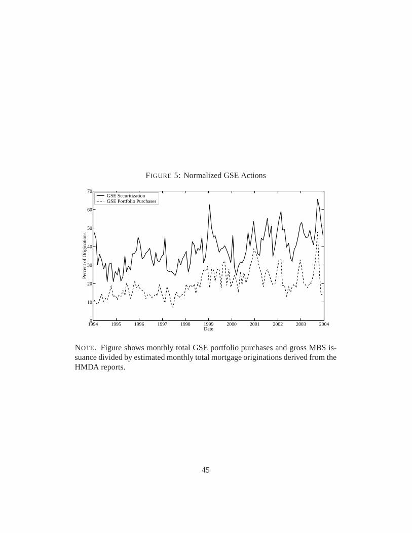
FIGURE 5: Normalized GSE Actions

1994 1995 1996 1997 1998 1999 2000 2001 2002 2003 20040

10

20

30

40

50

60

70

Date

Per

cent

of O

rigin

atio

ns

GSE SecuritizationGSE Portfolio Purchases

NOTE. Figure shows monthly total GSE portfolio purchases and gross MBS is-suance divided by estimated monthly total mortgage originations derived from theHMDA reports.

45

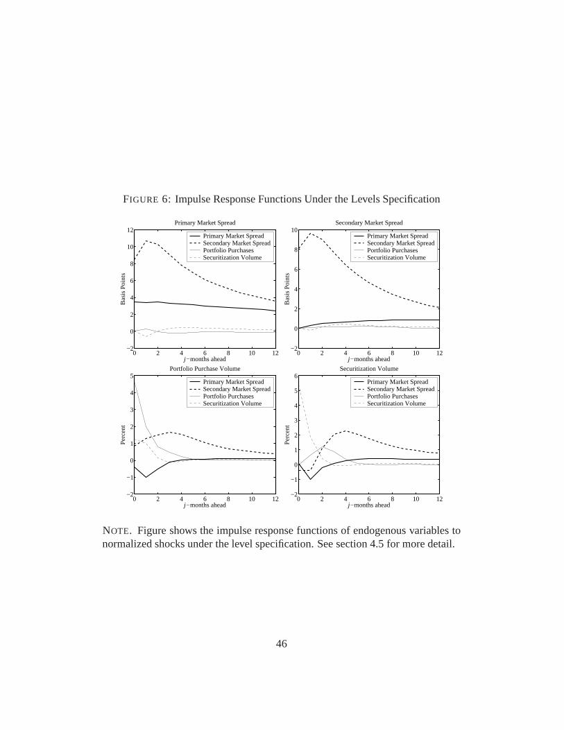
FIGURE 6: Impulse Response Functions Under the Levels Specification

0 2 4 6 8 10 12−2

0

2

4

6

8

10


j− months ahead

Bas

is P

oint

s


0 2 4 6 8 10 12−2

0

2

4

6

8


j− months ahead

Bas

is P

oint

s


0 2 4 6 8 10 12−2

−1

0

1

2

3

4


j− months ahead

Per

cent


0 2 4 6 8 10 12−2

−1

0

1

2

3

4

5


j− months ahead

Per

cent


NOTE. Figure shows the impulse response functions of endogenous variables tonormalized shocks under the level specification. See section 4.5 for more detail.

46

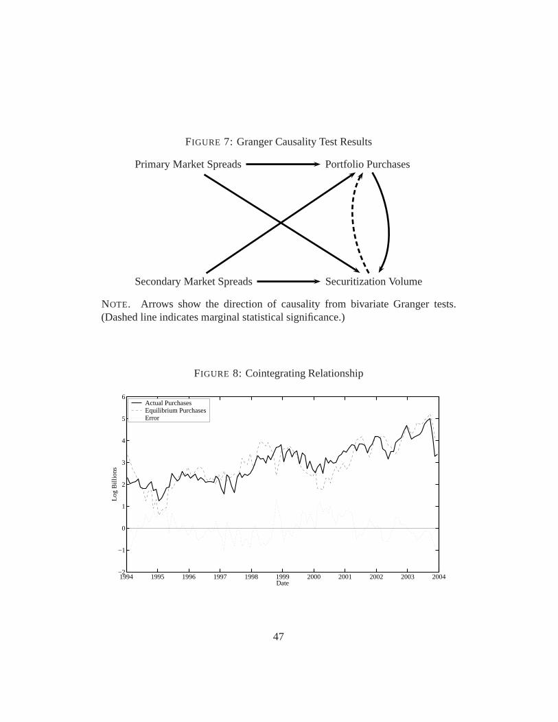
FIGURE 7: Granger Causality Test Results

Primary Market Spreads Portfolio Purchases

Secondary Market Spreads Securitization Volume

NOTE. Arrows show the direction of causality from bivariate Granger tests.(Dashed line indicates marginal statistical significance.)

FIGURE 8: Cointegrating Relationship

1994 1995 1996 1997 1998 1999 2000 2001 2002 2003 2004−2

−1

0

1

2

3

4

5

6

Date

Log

Bill

ions

Actual PurchasesEquilibrium PurchasesError

47

Documents

GSEs, Mortgage Rates, and Secondary Market … · GSEs, Mortgage Rates, and Secondary Market Activities Andreas Lehnert, Wayne Passmore, and Shane M. Sherlund 2005-07 ... GSE portfoliosis