University of Pretoria Department of Economics Working Paper Series

Growth Theory and Application: The Case of South Africa Dave Liu University of Pretoria Working Paper: 2007-14 September 2007 __________________________________________________________ Department of Economics University of Pretoria 0002, Pretoria South Africa Tel: +27 12 420 2413 Fax: +27 12 362 5207

GROWTH THEORY AND APPLICATION:

THE CASE OF SOUTH AFRICA

Guangling “Dave” Liu∗

September 2007

Abstract

This essay is a comparison study of traditional Neoclassical growth theory and

new growth theory. It also discusses growth theory in the real world by

investigating the so called “growth miracles” and “growth disasters” scenarios in

the developing world. Finally, the essay performs a standard growth accounting

exercise on South African economy mainly focuses on the importance of human

capital in growth process. Growth accounting exercise shows that South Africa

experiences a capital-accumulated growth in the 1970s and 80s, while sharply

shifts to technology-accumulated growth in the 1990s and early 2000s.

JEL Classification: O32, O40, O47, O49, O55

Keywords: Economic growth, Solow growth model, Growth accounting

∗ Ph.D. Candidate, Department of Economics, University of Pretoria, Pretoria, 0002, South Africa, Email:

dave.liu@up.ac.za. Phone: +27 12 420 3729, Fax: +27 12 362 5207.

2

1. INTRODUCTION

“To account for sustained growth, the modern theory needs to postulate

continuous improvements in technology or in knowledge or in human capital

(I think these are all just different terms for the same thing) as an ‘engine of

growth’.” (Lucas, 2003: [9])

Over the past few centuries, output growth has been raising world widely.

However, cross-country income differences on average have been widened.

Economists use the word “growth miracles” and “growth disasters” to illustrate

output growth differs in individual countries. The scenarios of Japan from the end

of World War Two and “four tigers”1 from 1960 are referred to “growth miracles”.

The income per capita of the “four tigers” increased more than fourfold from 1960

to 1990. On the other side, scenarios in many Sub-Saharan African countries

during the same time period are regarded as “growth disasters”. During the time

period from 1965 to 1990, the growth rate of income per capita of Sub-Saharan

Africa is 0.5 percent, while the figure of other less developed countries is 1.7

percent (Collier and Gunning, 1999: 6).

The objective of this essay is to first have a comparison study of traditional

Neoclassical growth theory and new growth theory. The essay is then to discuss

growth theory in the real world by investigating the so called “growth miracles”

and “growth disasters” scenarios in the developing world. Finally, the essay

performs a standard growth accounting exercise on South African economy

mainly focuses on the importance of human capital in growth process since

human capital is a key means of improving the economic growth in the long run.

Besides the introduction and conclusion, the essay is organized as follows:

Section 2 and 3 review the traditional Neoclassical growth theory as well as the

new growth theory. Section 4 applies growth accounting technique to investigate

the growth performance of the South African economy.

1 Four tigers: Hong Kong, South Korea, Singapore, and Taiwan.

3

2. TRADITIONAL NEOCLASSICAL GROWTH THEORY

2.1 The Solow Growth Model

The Neoclassical growth model developed by Solow (1956) is built on production

function with constant returns to scale (CRS, hereafter) in its two arguments,

capital and labor:

),( ttt LKFY = (2.1)

The notation is as same as in the textbook, where Y is output, K capital, and L

labor. L is assumed to grow at rate of n , exogenously:

nL

L

t

t +=+ 11 (2.2)

The assumption of CRS says:

YLKFLKF λλλλ == ),(),( (2.3)

And it makes easier to work with the production function in intensive form:

)1,(),(L

KF

L

L

L

KF

L

Y== (2.4)

By definingL

Yy = ,

L

Kk = , and )1,()( kFkf = , (2.4) can be written as:

)(kfy = (2.5)

The intensive form of production function says that the output per unit of labor, y ,

is a function of the amount of capital per unit of labor, k . It implies that

y depends only on the quantity of k , regardless of the overall size of the

economy (Romer, 2006:10).

The model assumes that a constant fraction of output, s , is invested, that is,

sYS = . Further assuming the existing capital depreciates at rate, δ , the

competitive equilibrium of the Solow model can be written as the following:

])()([1

11 tttt knksf

nkk +−

+=−+ δ (2.6)

4

This equation states that the change in capital stock per unit of labor, the left-

hand side of the equation, is determined by two terms in the right-hand side of

the equation, where the first term, )( tksf , is the actual investment per unit of

labor, and the second term, tkn)( +δ , is the so called breakeven investment, the

amount of capital stock must be invested to keep the capital per unit of labor at

its existing level. In steady state:

tt kk =+1 ⇒ tt knksf )()( += δ (2.7)

When the actual investment per unit of labor exceeds the breakeven

investment, 01 >−+ tt kk , k increases until it reaches the steady state level, and

vice versa. Eventually, k will converge to its steady state level regardless where

it starts (Romer, 2006).

In the long run, when the economy converges to its steady state level of capital

stock per unit of labor, real output is growing at the same rate as population

growth rate, n . That is,

t

t

t

t

L

Y

L

Y=

+

+

1

1 ⇒ )1(11 nL

L

Y

Y

t

t

t

t +== ++ (2.8)

Given the assumption of constant growth rates of saving rate, population growth

rate, and the CRS, Solow growth model states that growths in key

macroeconomic variables are determined by the population growth rate.

In his classical paper, Solow (1956) also extends the basic model with technical

progress, A , which is assumed to growth at a constant rate, g . The technical

progress and labor enter into the production function multiplicatively2:

)( , tttt LAKFY = (2.9)

In steady state, growths in key macroeconomic variables are determined by the

growth rates of population and technical progress:

)1)(1(111 gnLA

LA

Y

Y

tt

tt

t

t ++== +++ (2.10)

2 So called labour-augmenting or Harrod-neutral.

5

Both basic Solow model and Solow model with technical progress are exogenous

growth models. The Solow growth model predicts that the long run improvement

of living standard depends on the economy’s fundamental characteristics

including the population growth rate, the savings rate, the rate of technical

progress, and the rate of capital depreciation. Therefore the structural policy

implication for traditional Neoclassical growth models are the following: reducing

the growth rate of population; encouraging saving; promoting technology and

reducing the depreciation rate of capital.

Capital accumulation plays an important role in the Solow growth model. It is the

only endogenous factor of production. Capital is however determined by the

saving rate exogenously. In the Solow model, saving rate is the most likely

parameter that policy can affect. An increase in the saving rate causes an

increase in the output per unit of labor. Romer (2006) emphasizes that this

increase in saving rate only causes an increase in the level of output per unit of

labor not the growth rate. Indeed, aggregate output, aggregate consumption, and

aggregate investment grow at the same rate at the labor force growth rate, n .

The real output per unit of labor is not growing in the long run!3

The diminishing marginal return to capital assures the “conditional convergence"

of capital per unit of labor. Since the intensive form of production function implies

that output per unit of labor depends only on the quantity of capital per unit of

labor regardless of the overall size of the economy, countries have roughly the

same fundamental characteristics should converge to similar steady state levels

of output per unit of labor. In addition, the “conditional convergence” property

implies that the initially “poor” 4 countries grow faster than the initially “rich”

countries (Agenor and Montiel, 1999: 673).

3 In the Solow model with technical progress, the growth rate of real output per unit of labour is

determined solely by the rate of technical progress, g . 4 In terms of capital per unit of labour.

6

2.2 Solow Model in the Real World

Does the traditional Neoclassical growth model explain the scenarios of “growth

miracles” and “growth disasters” discussed in the beginning of this section? This

section is to answer the question by employing growth accounting literature as

well as empirical evidence.

Growth accounting literature (Solow, 1957) provides a simple way of

decomposing output growth into different factors in the aggregate production

function:

)( 1 αα −= LKzFY ; 10 << α (2.11)

where α is the fraction of output that is contributed by the capital input, and

α−1 is the fraction that is contributed by the labor input. Output growth is

segregated into three factors, the capital input ,K the labor input ,L and the total

factor productivity z5 . Total factor productivity (TFP hereafter) is also called

“Solow residual” since it is measured as a residual in the Cobb-Douglas

production function:

αα −=

1LK

Yz (2.12)

As a residual, TFP captures the rest factors other than capital and labor input,

such as technical change, the relative price change of energy, and so on. One

key insight of the Solow growth model is that if the growth in TFP continues,

capital per unit of labor will increase continuously. So does output per unit of

labor. This is because given the quantity of capital and labor input, an increase in

TFP will increase the marginal product of labor.

Given the fact that real output per unit of labor is not growing in steady state,

macroeconomists may consider that the Eastern Asian “growth miracles” is

mainly driven by higher TFP than the rest of world. However, empirical evidence

suggests that the Eastern Asia’s rapid growth does not appear to have been a

5 Solow refers it as “technical change” in his 1957 paper.

7

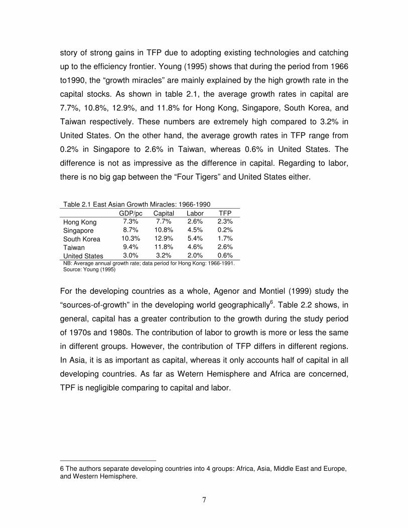
story of strong gains in TFP due to adopting existing technologies and catching

up to the efficiency frontier. Young (1995) shows that during the period from 1966

to1990, the “growth miracles” are mainly explained by the high growth rate in the

capital stocks. As shown in table 2.1, the average growth rates in capital are

7.7%, 10.8%, 12.9%, and 11.8% for Hong Kong, Singapore, South Korea, and

Taiwan respectively. These numbers are extremely high compared to 3.2% in

United States. On the other hand, the average growth rates in TFP range from

0.2% in Singapore to 2.6% in Taiwan, whereas 0.6% in United States. The

difference is not as impressive as the difference in capital. Regarding to labor,

there is no big gap between the “Four Tigers” and United States either.

Table 2.1 East Asian Growth Miracles: 1966-1990

GDP/pc Capital Labor TFP

Hong Kong 7.3% 7.7% 2.6% 2.3%

Singapore 8.7% 10.8% 4.5% 0.2%

South Korea 10.3% 12.9% 5.4% 1.7%

Taiwan 9.4% 11.8% 4.6% 2.6%

United States 3.0% 3.2% 2.0% 0.6% NB: Average annual growth rate; data period for Hong Kong: 1966-1991. Source: Young (1995)

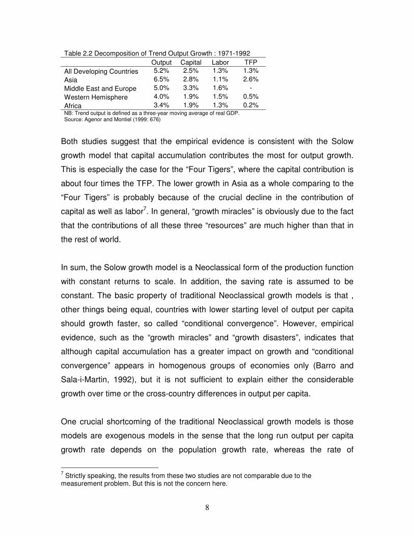
For the developing countries as a whole, Agenor and Montiel (1999) study the

“sources-of-growth” in the developing world geographically6. Table 2.2 shows, in

general, capital has a greater contribution to the growth during the study period

of 1970s and 1980s. The contribution of labor to growth is more or less the same

in different groups. However, the contribution of TFP differs in different regions.

In Asia, it is as important as capital, whereas it only accounts half of capital in all

developing countries. As far as Wetern Hemisphere and Africa are concerned,

TPF is negligible comparing to capital and labor.

6 The authors separate developing countries into 4 groups: Africa, Asia, Middle East and Europe, and Western Hemisphere.

8

Table 2.2 Decomposition of Trend Output Growth : 1971-1992

Output Capital Labor TFP

All Developing Countries 5.2% 2.5% 1.3% 1.3%

Asia 6.5% 2.8% 1.1% 2.6%

Middle East and Europe 5.0% 3.3% 1.6% -

Western Hemisphere 4.0% 1.9% 1.5% 0.5%

Africa 3.4% 1.9% 1.3% 0.2% NB: Trend output is defined as a three-year moving average of real GDP. Source: Agenor and Montiel (1999: 676)

Both studies suggest that the empirical evidence is consistent with the Solow

growth model that capital accumulation contributes the most for output growth.

This is especially the case for the “Four Tigers”, where the capital contribution is

about four times the TFP. The lower growth in Asia as a whole comparing to the

“Four Tigers” is probably because of the crucial decline in the contribution of

capital as well as labor7. In general, “growth miracles” is obviously due to the fact

that the contributions of all these three “resources” are much higher than that in

the rest of world.

In sum, the Solow growth model is a Neoclassical form of the production function

with constant returns to scale. In addition, the saving rate is assumed to be

constant. The basic property of traditional Neoclassical growth models is that ,

other things being equal, countries with lower starting level of output per capita

should growth faster, so called “conditional convergence”. However, empirical

evidence, such as the “growth miracles” and “growth disasters”, indicates that

although capital accumulation has a greater impact on growth and “conditional

convergence” appears in homogenous groups of economies only (Barro and

Sala-i-Martin, 1992), but it is not sufficient to explain either the considerable

growth over time or the cross-country differences in output per capita.

One crucial shortcoming of the traditional Neoclassical growth models is those

models are exogenous models in the sense that the long run output per capita

growth rate depends on the population growth rate, whereas the rate of

7 Strictly speaking, the results from these two studies are not comparable due to the

measurement problem. But this is not the concern here.

9

technology progress in the Solow growth model with technology progress.

Therefore, the model itself can neither explain the mechanisms that generate

long run growth, nor evaluate the efficiency of government growth policies.

10

3. NEW GROWTH THEORY

The traditional Neoclassical growth models became more and more technical

and lack of empirical applications (eg. the Ramsey-Cass-koopmans model).

During the time period from the late 1960s to early 1980s, macroeconomic

research shifted from long run growth theory to the short run fluctuations, and

business cycle models with rational expectations (Barro and Sala-i-Martin, 1995:

12). Since the mid-1980s, new growth theory (Romer, 1986, 1990; Lucas, 1988)

addresses the limitations of the Neoclassical model by proposing two main

channels, human capital and knowledge, through which long run growth is

generated endogenously.

3.1 The Solow Growth Model with Human Capital

The growth model presented here consists of introducing human capital as an

additional production input which is accumulated in the same way as physical

capital. Every year a constant share of output is invested in education, training of

the labor force, i.e. human capital. In contract to Lucas (1988) that production

function of human capital differs from other goods, here, human capital, physical

capital, and consumption are produced by same technologies (Mankiw et al,

1992: 416). The production function takes the form:

θαθα −−= 1)(ALHKY ; ,10 << θ 1<+θα 8 (3.1)

where H is the stock of human capital, and other variables are defined as in the

previous section. Households now choose the fractions of their income to

consume and invest in physical or human capital. Assuming both physical and

8 1<+θα , implies decreasing returns to K and H . The Solow model with human capital

becomes endogenous if constant returns to scale applies, 1=+ θα (see Mankiw, et al, 1992).

11

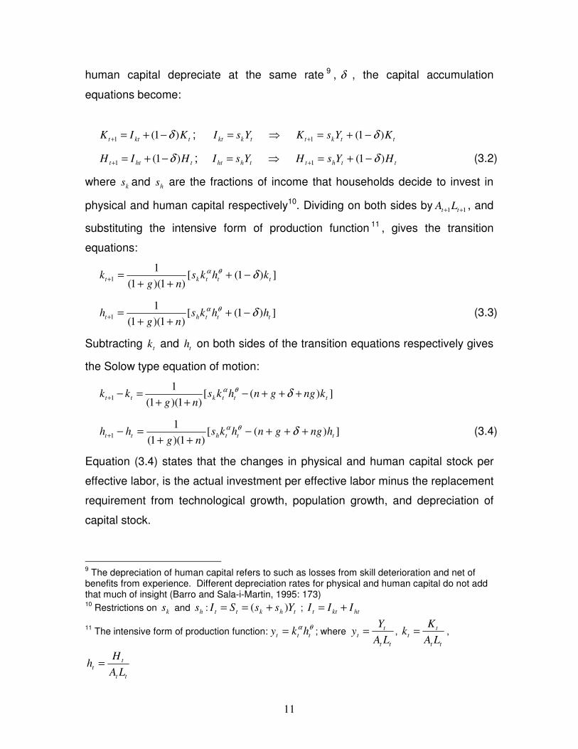
human capital depreciate at the same rate 9 , δ , the capital accumulation

equations become:

tktt KIK )1(1 δ−+=+ ; tkkt YsI = ⇒ ttkt KYsK )1(1 δ−+=+

thtt HIH )1(1 δ−+=+ ; thht YsI = ⇒ ttht HYsH )1(1 δ−+=+ (3.2)

where ks and hs are the fractions of income that households decide to invest in

physical and human capital respectively10. Dividing on both sides by 11 ++ tt LA , and

substituting the intensive form of production function 11 , gives the transition

equations:

])1([)1)(1(

11 tttkt khks

ngk δθα −+

++=+

])1([)1)(1(

11 tttht hhks

ngh δθα −+

++=+ (3.3)

Subtracting tk and th on both sides of the transition equations respectively gives

the Solow type equation of motion:

])([)1)(1(

11 tttktt knggnhks

ngkk +++−

++=−+ δθα

])([)1)(1(

11 ttthtt hnggnhks

nghh +++−

++=−+ δθα (3.4)

Equation (3.4) states that the changes in physical and human capital stock per

effective labor, is the actual investment per effective labor minus the replacement

requirement from technological growth, population growth, and depreciation of

capital stock.

9 The depreciation of human capital refers to such as losses from skill deterioration and net of

benefits from experience. Different depreciation rates for physical and human capital do not add that much of insight (Barro and Sala-i-Martin, 1995: 173) 10

Restrictions on ks and hs : thktt YssSI )( +== ; htktt III +=

11 The intensive form of production function:

θαttt hky = ; where

tt

tt

LA

Yy = ,

tt

tt

LA

Kk = ,

tt

tt

LA

Hh =

12

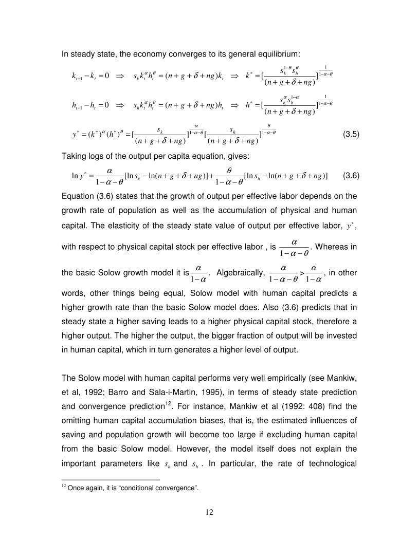
In steady state, the economy converges to its general equilibrium:

01 =−+ tt kk ⇒ tttk knggnhks )( +++= δθα ⇒ θα

θθ

δ−−

−∗

+++= 1

11

])(

[nggn

ssk hk

01 =−+ tt hh ⇒ ttth hnggnhks )( +++= δθα ⇒ θα

αα

δ−−

−∗

+++= 1

11

])(

[nggn

ssh hk

θα

θ

θα

αθα

δδ−−−−∗∗∗

++++++== 11 ]

)([]

)([)()(

nggn

s

nggn

shky hk (3.5)

Taking logs of the output per capita equation, gives:

)]ln([ln1

)]ln([ln1

ln nggnsnggnsy hk +++−−−

++++−−−

=∗ δθα

θδ

θα

α (3.6)

Equation (3.6) states that the growth of output per effective labor depends on the

growth rate of population as well as the accumulation of physical and human

capital. The elasticity of the steady state value of output per effective labor, ∗y ,

with respect to physical capital stock per effective labor , is θα

α

−−1. Whereas in

the basic Solow growth model it isα

α

−1. Algebraically,

θα

α

−−1>

α

α

−1, in other

words, other things being equal, Solow model with human capital predicts a

higher growth rate than the basic Solow model does. Also (3.6) predicts that in

steady state a higher saving leads to a higher physical capital stock, therefore a

higher output. The higher the output, the bigger fraction of output will be invested

in human capital, which in turn generates a higher level of output.

The Solow model with human capital performs very well empirically (see Mankiw,

et al, 1992; Barro and Sala-i-Martin, 1995), in terms of steady state prediction

and convergence prediction12. For instance, Mankiw et al (1992: 408) find the

omitting human capital accumulation biases, that is, the estimated influences of

saving and population growth will become too large if excluding human capital

from the basic Solow model. However, the model itself does not explain the

important parameters like ks and hs . In particular, the rate of technological

12

Once again, it is “conditional convergence”.

13

process, g , which determines the long run growth rate per effective labor

remains unexplained. The following section illustrates how the Solow model with

research and development (R&D) resolves this issue.

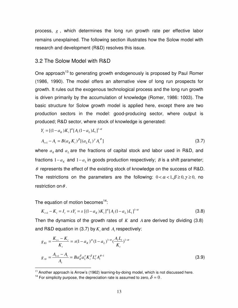
3.2 The Solow Model with R&D

One approach13 to generating growth endogenously is proposed by Paul Romer

(1986, 1990). The model offers an alternative view of long run prospects for

growth. It rules out the exogenous technological process and the long run growth

is driven primarily by the accumulation of knowledge (Romer, 1986: 1003). The

basic structure for Solow growth model is applied here, except there are two

production sectors in the model: good-producing sector, where output is

produced; R&D sector, where stock of knowledge is generated:

αα −−−= 1])1([])1[( tLttKt LaAKaY

])[()(1

θγβttLtKtt ALaKaBAA =−+ (3.7)

where Ka and La are the fractions of capital stock and labor used in R&D, and

fractions Ka−1 and La−1 in goods production respectively; B is a shift parameter;

θ represents the effect of the existing stock of knowledge on the success of R&D.

The restrictions on the parameters are the following: ,0,0,10 ≥≥<< γβα no

restriction onθ .

The equation of motion becomes14:

ssYIKK tttt ===−+1

αα −−− 1])1([])1[( tLttK LaAKa (3.8)

Then the dynamics of the growth rates of K and A are derived by dividing (3.8)

and R&D equation in (3.7) by tK and tA respectively:

ααα −−+ −−=−

= 11 )()1()1(t

ttLK

t

ttKt

K

LAaas

K

KKg

11 −+ =−

= θγβγβtttLK

t

ttAt ALKaBa

A

AAg (3.9)

13

Another approach is Arrow’s (1962) learning-by-doing model, which is not discussed here. 14

For simplicity purpose, the depreciation rate is assumed to zero, 0=δ .

14

where Ktg and Atg represent growth rate of capital stock and knowledge.

Defining αα −−−= 1)1()1( LKK aasc , γβLKA aBac = , and taking logs of both sides of

equation Kg and Ag , gives:

]lnln)[ln1(lnln tttKKt KLAcg −+−+= α

tttAAt ALKcg ln)1(lnlnlnln −+++= θγβ (3.10)

Therefore:

))(1()]ln(ln)ln(ln)ln)[(ln1(lnln 1111 KAttttttKtKt gngKKLLAAgg −+−=−−−+−−=− −−−− αα

AkttttttAtAt gngAALLKKgg )1()ln)(ln1()ln(ln)ln(lnlnln 1111 −++=−−+++−=− −−−− θγβθγβ

(3.11)

In steady state:

0lnln 1 =− −KtKt gg ⇒ ngg AK += ∗∗ (3.12)

0lnln 1 =− −AtAt gg ⇒ ∗∗ −+−= AK g

ng

β

θ

β

γ 1 (3.13)

Substituting (3.12) into (3.13) gives the steady state values of Ag and Kg :

ng Aβθ

βγ

−−

+=

1

* ; ngKβθ

θγ

−−

−+=

1

1* (3.14)

In steady state, the output growth rate is:

ngYYg Atty +=−= −*

1

* lnln (3.15)15

Equation (3.15) together with (3.12) implies that in equilibrium16 K and A are

growing at rates shown in (3.14), and output is growing at the same rate as

capital, **

Ky gg = . Output per capita is growing at rate *

Ag (Romer, 2006: 111).

The Solow growth model with R&D is an endogenous growth model in the sense

that the long run growth rate is constant and determined within the model,

nggg AKy +== *** , where the growth of knowledge is determined by parameters,

15

]ln)1ln()[ln1(]ln)1[ln(ln tLttKt LaAKaY +−+−++−= αα ⇒

ngngng

nggLLAAKKYY

AAA

AKtttttttt

+=+−++=

+−+=−+−−+−=− −−−−

))(1()(

))(1()ln(ln)ln)[(ln1()ln(lnlnln 1111

αα

αααα

16

The necessary condition to guarantee the equilibrium exists is 1<+θβ (Romer, 2006:110).

15

,β γ , and θ . Neither the fractions of labor force and capital stock engaged in

R&D, La and Ka , nor does the saving rate, s , have effect on the long run growth

(Romer, 2006: 111).

3.3 Neoclassical vs. New Growth Theory

The traditional Neoclassical growth models play a major and essential role in the

development of dynamic general equilibrium analysis. However, as a theory of

growth, it fails to explain the basic facts of actual growth behavior. Also empirical

evidence indicates a persistent different per capita growth rates over long period

across nations, i.e. the “conditional convergence” does not appear (McCallum,

1996: 50-52). One explanation of this can be the fact that different countries may

not be able to access the same technology. Generally speaking, the technology

level in developed countries is relatively higher than that in developing countries.

Also the technological innovation often occurs in developed countries and

countries who own new technologies usually prevent them from being adopted

by others. Even though assuming the new technologies were able to be

accessed by other countries, there is always a long time lag. This difference in

technology process can explain the persistent differences in the standards of

living across nations. Williamson (2005: 213-218) argues that there are two good

reasons why significant barriers to the adoption of new technology exist. First, a

powerful union has a strong incentive to prevent its members losing jobs due to

their obsolete skills made by new technologies. The second one is the trade

restrictions introduced by government in order to shield domestic infantile

industries from foreign competition, which are the cases in most of the

developing countries. These barriers reduce the incentive of technological

innovations and have a negative effect on total factor productivity.

Alternatively new growth theory models explain the failure of “conditional

convergence” by proposing the externalities and spillover effects of human

capital and knowledge. Human capital is the accumulated stock of skills and

16

education embodied in labor force. Empirical literature takes education

(schooling) as a proxy of human capital. The externality of human capital exists

because public learning or education increases the stock of human capital of

labor force. A more highly skilled labor force becomes more productive, and

hence produces more. In addition, individuals who have higher skills can pass on

their skills to others, therefore the higher level of human capital, the more

efficient the human capital accumulates. Intuitively, since the skills of the labor

force is an important input factor, adding human capital to the Solow model

improves the growth model itself.

Empirics suggest that investing in human capital is as important as investing in

physical capital. However, for households, there are associated opportunity costs

for them to invest in human capital. For instance, the opportunity cost of investing

in education takes the form of forgone labor earning. The opportunity cost varies

from individual to individual. It is much higher for an individual with more human

capital than the one with little.

The virtue of new growth theory models is attempting to explain growth

endogenously. However as argued by MaCallum (1996), there is a logical

difficulty with these models. As human capital cannot be separated from labor

force, it is a private good and rival. Therefore, the accumulated human capital

which generates the never-ending growth in the Lucas model cannot be

automatically passed on to workers in succeeding generations. In contrast,

knowledge is semi-public good 17 . Unlike human capital, an individual’s

acquisition of knowledge does not prevent others to acquire the same knowledge.

Knowledge is “semi” public good in the sense that new knowledge can be

partially or temporarily kept secret due to the patent and certain degree of

monopoly power owned by individuals or firms who engaged in the innovation of

new knowledge (Romer, 1990). Thus as shown by (3.15), it is the accumulated

17

Some authors refer knowledge is completely nonrival in favour of discussing the spillover effects of knowledge.

17

knowledge which can be passed on from generation to generation, can plausibly

generate the never-ending growth endogenously (also see McCallum, 1996: 59-

61; Grossman and Helpman, 1994: 35). Nevertheless, it is important to realize

that:

“Growth in the stock of useful knowledge does not generate sustained

improvement in living standards unless it raises the return to investing in

human capital in most families. This condition is a statement about the nature

of the stock of knowledge that is required, about the kind of knowledge that is

‘useful.’ But more centrally, it is a statement about the nature of the society.”

(Lucas, 2001: [3])

18

4. THE SOUTH AFRICAN CONTEXT

4.1 A Standard Growth Accounting Exercise

In order to explain South Africa’s economic growth over the last few decades, a

first step is to identify the relative contributions of capital, labor, and the overall

productivity. The methodology on which the standard growth accounting exercise

is based on can be described as follows (Solow, 1957; Barro, 1998):

αα −= 1)(HLzKY (4.1)

where z represents TFP, α and α−1 refer to the share of physical capital and

labor respectively in national output18, Y , K , and L are output, physical capital

and labor respectively. H is the human capital measure which takes the form as

the following:

SH )07.1(= (4.2)

where s is the average years of schooling. The series of average years of

schooling is generated based on the censuses of 1985, 1991, 1996, and 2001

(Louw et al, 2006). The return to schooling for each year is assumed at 7

percent19, which is a value near the lower boundary of the results from the

microeconomics studies (Bosworth and Collins, 2003).

Solow (1957) shows that (4.1) yields the following identity:

lkyz ˆ)1(ˆˆˆ αα −−−= (4.3)20

where lower letter with a hat denotes growth rate. The growth rates of TFP are

obtained from the discrete version of (4.2). Data for the TFP decompositions are

18

Given the assumption of perfect competition and CRS, capital and labor output share sum to unity. 19

Using a global data set, coving 95 countries, Cohen and Soto (2001) estimate returns to schooling in the

range of 7 to 10 percent, close to the average of the microeconomic studies. Also see du Plessis and Smit

(2006).

20

Both labor adjusted and not adjusted for changes in human capital are considered in the growth

accounting exercise.

19

drawn from the South African Reserve Bank (SARB) and Trade and Industry

Policy Secretariat (TIPS) data bases.

Alternatively, Liu and Gupta (2006) use a version of Hansen’s real business cycle

benchmark model to calibrate the South African economy. The authors obtain the

calibrated capital output share, 0.26. This number is relatively small compared to

0.48, which is computed based on the data from TIPS.

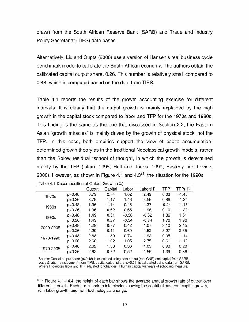
Table 4.1 reports the results of the growth accounting exercise for different

intervals. It is clearly that the output growth is mainly explained by the high

growth in the capital stock compared to labor and TFP for the 1970s and 1980s.

This finding is the same as the one that discussed in Section 2.2, the Eastern

Asian “growth miracles” is mainly driven by the growth of physical stock, not the

TFP. In this case, both empirics support the view of capital-accumulation-

determined growth theory as in the traditional Neoclassical growth models, rather

than the Solow residual “school of though”, in which the growth is determined

mainly by the TFP (Islam, 1995; Hall and Jones, 1999; Easterly and Levine,

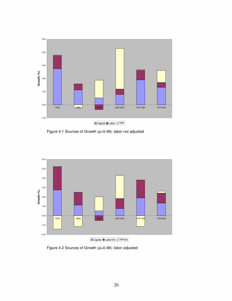
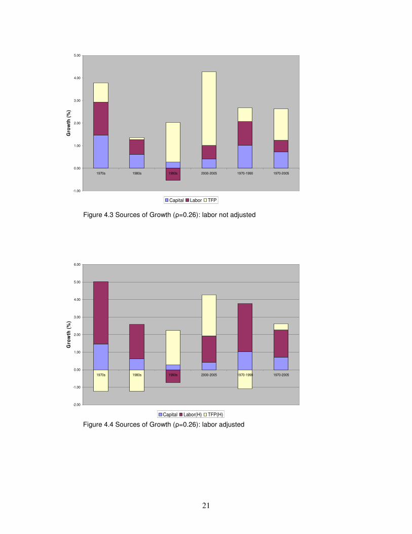
2000). However, as shown in Figure 4.1 and 4.321, the situation for the 1990s

Table 4.1 Decomposition of Output Growth (%)

Output Capital Labor Labor(H) TFP TFP(H)

ρ=0.48 3.79 2.74 1.02 2.49 0.03 -1.43 1970s

ρ=0.26 3.79 1.47 1.46 3.56 0.86 -1.24

ρ=0.48 1.36 1.14 0.45 1.37 -0.24 -1.16 1980s

ρ=0.26 1.36 0.62 0.65 1.96 0.10 -1.22

ρ=0.48 1.49 0.51 -0.38 -0.52 1.36 1.51 1990s

ρ=0.26 1.49 0.27 -0.54 -0.74 1.76 1.96

ρ=0.48 4.29 0.77 0.42 1.07 3.10 2.45 2000-2005

ρ=0.26 4.29 0.41 0.60 1.52 3.27 2.35

ρ=0.48 2.68 1.89 0.74 1.92 0.05 -1.14 1970-1990

ρ=0.26 2.68 1.02 1.05 2.75 0.61 -1.10

ρ=0.48 2.62 1.33 0.36 1.09 0.93 0.20 1970-2005

ρ=0.26 2.62 0.72 0.52 1.55 1.39 0.36

Source: Capital output share (ρ=0.48) is calculated using data output (real GNP) and capital from SARB, wage & labor (employment) from TIPS; capital output share (ρ=0.26) is calibrated using data from SARB. Where H denotes labor and TFP adjusted for changes in human capital via years of schooling measure.

21

In Figure 4.1 – 4.4, the height of each bar shows the average annual growth rate of output over different intervals. Each bar is broken into blocks showing the contributions from capital growth, from labor growth, and from technological change.

20

-1.00

0.00

1.00

2.00

3.00

4.00

5.00

1970s 1980s 1990s 2000-2005 1970-1990 1970-2005

Gro

wth

(%

)

Capital Labor TFP

Figure 4.1 Sources of Growth (ρ=0.48): labor not adjusted

-2.00

-1.00

0.00

1.00

2.00

3.00

4.00

5.00

6.00

1970s 1980s 1990s 2000-2005 1970-1990 1970-2005

Grw

oth

(%

)

Capital Labor(H) TFP(H)

Figure 4.2 Sources of Growth (ρ=0.48): labor adjusted

21

-1.00

0.00

1.00

2.00

3.00

4.00

5.00

1970s 1980s 1990s 2000-2005 1970-1990 1970-2005

Gro

wth

(%

)

Capital Labor TFP

Figure 4.3 Sources of Growth (ρ=0.26): labor not adjusted

-2.00

-1.00

0.00

1.00

2.00

3.00

4.00

5.00

6.00

1970s 1980s 1990s 2000-2005 1970-1990 1970-2005

Gro

wth

(%

)

Capital Labor(H) TFP(H)

Figure 4.4 Sources of Growth (ρ=0.26): labor adjusted

22

and 2000-2005 are reversed. The contribution of TFP is -0.24

percent in the 1980s, while it turns to 1.36 percent in the 1990s22. Indeed, the

accumulation in TFP is the single strongest contributor to the output growth (1.49

percent) in the 1990s. This situation continues to 2000-2005, where the

accumulation in TFP is 3.10 percent and output growth is 4.29 percent. In terms

of the whole study period, both capital accumulation and TFP growth have made

important contributions to growth.

4.2 Human Capital

Besides the finding that the source of growth has significantly shifted from capital

accumulation to the TFP growth over time, the growth accounting exercise also

shows that the decomposition is sensitive to underlying assumptions of the

production factors23. Labor adjusted for changes in human capital affects the

result of the decomposition of growth. The contribution of labor increases

significantly after adjusted for human capital in 1970s and 1980s, which in turn

results that output growth is explained by both capital and labor. The labor

adjustment effect is minimal in the 1990s. In terms of the whole study period,

capital and labor are the main sources of growth, and there is little role for TFP.

But, in 1990s and 2000-2005, TFP still contributes the most to growth. Moreover,

there is a significant increase in TFP accumulation in 2000-2005, which indicates

the same finding in the case of labor unadjusted for changes in human capital.

Increases in education could affect economic growth through two different

channels. First, microeconomic studies suggest more education may improve the

productivity of the workers. Second, Mankiw et al (1992) introduce human capital

(education) as an independent factor in growth process. The authors argue that

as machines and capital increasingly substitute for the raw force of labor, human

capital is the most important production factor nowadays. An educated worker is

more capable to implement new technologies and improve efficiency than an

22

For the capital output share of 0.48 and unadjusted labor. 23

See Figure 4.1 and 4.2.

23

uneducated worker. Thus, both approaches assume a positive correlation

between gains in education and growth. However, recent macroeconomic studies

(Barro and Lee, 2000; Bils and klenow, 2000; Easterly and Levine, 2001) fail to

find a significant positive correlation between gains in education and growth. The

failure to replicate the microeconomic results at the aggregate level might due to:

(1) the private return to education that underlines the micro-analysis is much

greater than the social return reflected in the aggregate data; (2) the variations in

the quality of education across countries (Bosworth and Collins, 2003).

The use of years of schooling as the measure of education attainment does not

incorporate any adjustment for variations in quality. In the international context,

the quality of education varies substantially across countries although it is difficult

to measure directly. In the South African context, there is a significant racial

difference in the quality of education24. It is widely believed that the African

education system provides inferior education in South Africa, due to “historically”

a combination of extremely high pupil-teacher ratios, poorly qualified teachers

and low financing levels (Moll, 1996). Racial differences in education have

decreased steadily over time since 1994. Nonetheless, as Fedderke (2001)

points out now South Africa spends far more than comparable developing

countries as a percentage of GDP on education, the problem is with little concern

for the deepening of the quality of education. School quality has been shown to

have a positive and significant effect on years of completed education. Investing

in human capital is a key means of improving the economic growth in the long

run. Moreover, the external effect of human capital is at the heart of the

endogenous growth literature (Case and Deaton, 1999).

4.3 Input Factor Elasticity

In the standard growth accounting exercise, the capital output shares are

obtained through two different approaches as explained above. Do the obtained

24

See Fedderke et al (2000) and Anderson et al (2001) for a discussion of historical differences in school

quality across racial groups.

24

two different values of capital output shares (0.48 vs. 0.26) matter? Comparing

Figure 4.1 to 4.3 (labor not adjusted for education) as well as Figure 4.2 to 4.4

(labor adjusted for education), the differences in terms of the contributions to

growth are minimal especially for the later case. The only relatively significant

effect appears in the 1970s and 1980s for the case of labor not adjusted for

education. There is a significant increase in TFP and decrease in labor

contribution to growth in the 1970s, while an inverse contribution of TFP in the

1980s although the absolute value is minor.

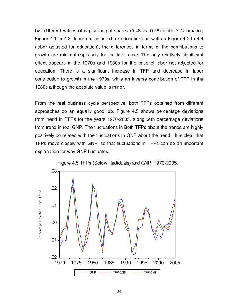
From the real business cycle perspective, both TFPs obtained from different

approaches do an equally good job. Figure 4.5 shows percentage deviations

from trend in TFPs for the years 1970-2005, along with percentage deviations

from trend in real GNP. The fluctuations in Both TFPs about the trends are highly

positively correlated with the fluctuations in GNP about the trend. It is clear that

TFPs move closely with GNP, so that fluctuations in TFPs can be an important

explanation for why GNP fluctuates.

-.02

-.01

.00

.01

.02

.03

1970 1975 1980 1985 1990 1995 2000 2005

GNP TFP(0.26) TFP(0.48)

Figure 4.5 TFPs (Solow Rediduals) and GNP, 1970-2005.

Pe

rce

nta

ge

De

via

tio

n F

rom

Tre

nd

25

5. CONCLUSION

Macroeconomists have responded with a rich literature on growth theory to the

vast differences in living standard over time and across countries. The traditional

Neoclassical growth theory does a nice job in explaining the “growth miracles”,

that is, the Eastern Asia’s rapid growth is mainly explained by the high growth

rate in the capital stock. However, the traditional Neoclassical growth models are

exogenous. The model itself can neither explain the mechanisms that generate

long run growth, nor explain the “conditional convergence”. Alternatively, new

growth theory models explain the failure of “conditional convergence” by

proposing the externalities and spillover effects of human capital and knowledge.

Growth accounting exercise shows that South Africa experiences a capital-

accumulated growth in the 1970s and 80s, while sharply shifts to technology-

accumulated growth in the 1990s and early 2000s. The standard growth

accounting approach applied in this essay is based on the assumption of

constant returns to scale. Since new growth (endogenous) theory is challenging

against this assumption, further study should be done in this regard.

26

REFERENCES

Agenor, P. R., and P. J., Montiel, 1999. Development Macroeconomics. 2nd

edition. Princeton university Press. Princeton, New Jersey.

Anderson, K., Case, A. and D. Lam, 2001. Causes and consequences of

schooling outcomes in South Africa: evidence from survey data. Population

Studies Center, Research Report, No. 01-490.

Barro, R. J. and X., Sala-i-Martin, 1992. Convergence. Journal of political

Economy, 100 (2): 223-251.

_, 1995. Economic Growth. First MIT Press ed. 1999. McGraw-Hill. New York.

_, 1998. Notes on growth accounting. Boston, MA: NBER Working Paper, 6654.

_, and J. W., Lee, 2000. International data in educational attainment, updates

and implications. Cambridge, MA: NBER Working Paper, 7911.

Bils, M. and P. J., Klenow, 2000. Does schooling cause growth? American

Economic Review, 90 (5): 1160-1183.

Bosworth, B. and S. M. Collins, 2003. The empirics of growth: an update.

Washington, Brookings institution mimeograph.

Case, A. and A. Deaton, 1999. School input and educational outcomes in South

Africa. Quarterly Journal of Economics, 114: 1047-1084.

Cohen, D. and M. Soto, 2001. Growth and human capital: good data, good

results. OECD, Technical Papers, 179.

27

Collier, P., and J. W., Gunning, 1999. Why has Africa grown slowly? Journal of

Economic Perspectives, 13 (3): 3-22.

Easterly, W. and R. Levine, 2000. It’s not factor accumulation: stylized facts and

growth models. World Bank Economic Review, 15 (2): 177-219.

Du plessis, S. A. and B. Smit, 2006 Economic growth in South Africa since 1994.

Stellenbosch Economic Working Papers: 1.

Fedderke, J. W., 2001. Technology, human capital and growth: evidence from a

middle income country case study applying dynamic heterogeneous panel

analysis. Econometric Research Southern Africa Policy Paper No. 23, University

of Witwatersrand.

_, 2002. The structure of growth in the South African economy: factor

accumulation and total factor productivity growth 1970-1997. South African

Journal of Economics, 70 (4): 612-646.

_, de Kadt, R. and J. M. Luiz, 2000. Uneducating South Africa: the failure to

address the 1910-1993 legacy. International Review of Education, 46 (July): 257-

281.

Grossman, G. M., and E., Helpman, 1994. Endogenous innovation in the theory

of growth. Journal of Economic Perspectives, 8 (1): 23-44.

Hall, R. E. and C. I. Jones, 1999. Why do some countries produce so much more

output per workers than others? Quarterly Journal of Economics, 114 (1): 83-116.

Islam, N., 1995. Growth empirics: a panel data approach. Quarterly Journal of

Economics, 110 (4): 1127-1170.

28

Liu, G. L. and R. Gupta, 2007. A small-scale DSGE model for forecasting the

South African economy. South African Journal of Economics, 75(2): 179-193.

Louw, M., Van der Berg, S. and D. Yu, 2006. Educational attainment and

intergenerational social mobility in South Africa. Stellenbosch, Economic Working

Paper, 09/06.

Lucas, R. E. Jr., 1988. On the mechanics of economic development. Journal of

Monetary Economics, 22 (1): 3-42.

_, 2001. “A million mutinies” the key to economic development. Federal Reserve

Bank of Minneapolis Article, December 2001. [on line] Available from:

http://minneapolisfed.org/pubs/region/01-12/lucas.cfm [Accessed: 2006-07-18]

_, 2003. The industrial revolution: past and future. Federal Reserve Bank of

Minneapolis, Annual report. [on line] Available from:

http://minneapolisfed.org/pubs/region/04-05/essay.cfm [Accessed: 2006-07-18]

Mankiw, N. G., Romer, D., and Weil, D. N., 1992. A contribution to the empirics

of economics growth. The Quarterly Journal of Economics, 107 (2): 407-437.

McCallum, B. T., 1996. Neoclassical vs. endogenous growth analysis: an

overview. Federal Reserve Bank of Richmond Economic Quarterly, 82 (4): 41-71.

Moll, P. G., 1996. The collapse of primary schooling returns in South Africa 1960-

1990. Oxford Bulletin of Economics and Statistics, 58 (1): 185-209.

Romer, D., 2006. Advanced Macroeconomics. 3rd edition. McGraw-Hill. New York.

Romer, P. M., 1986. Increasing returns and long-run growth. Journal of Political

Economy, 94 (5): 1002-1037.

29

_, 1990. Endogenous technological change. Journal of Political Economy, 98 (5),

part 2: 71-102.

Solow, R. M., 1956. A contribution to the theory of economic growth. The

Quarterly Journal of Economics, 70 (1): 65-94.

_, 1957. Technical change and the aggregate production function. The Review of

Economics and Statistics, 39(3): 312-320.

Williamson, S. D., 2005. Macroeconomics. 2nd edition. Pearson Addison Wesley.

Boston.

Young, A., 1995. The tyranny of numbers: confronting the statistical realities of

the East Asian growth experience. Quarterly Journal of Economics, 110: 641-680.