Grouting with high water/solid-ratios – Literature and laboratory study MAGNUS AXELSS ON GUNNAR GUSTAF SON Department of Civil and Environmental Engineering Division of GeoEngineering Research Group of Engineering Geology CHALMERS UNIVERSITY OF TECHNOLOGY GÖTEBORG, SWEDEN 2007 Report No. 2007:5

Report No. 2007:5

Grouting with high water/solid-ratios – Literature

and laboratory study

MAGNUS AXELSSON GUNNAR GUSTAFSON

Department of Civil and Environmental Engineering Division of GeoEngineering

Research Group of Engineering Geology CHALMERS UNIVERSITY OF TECHNOLOGY

Göteborg 2007

Grouting with high water/solid-ratios – Literature and laboratory study MAGNUS AXELSSON GUNNAR GUSTAFSON © MAGNUS AXELSSON AND GUNNAR GUSTAFSON, 2007 Publ. 2007:5 ISSN 1662-9162 Chalmers University of Technology Department of Civil and Environmental Engineering Division of GeoEngineering Research Group of Engineering Geology SE-412 96 Göteborg Sweden Phone: +46 (0) 31 772 1000 Chalmers reproservice Göteborg 2007

i

PREFACE This work was financed by Development Fund of the Swedish Construction Industry (SBUF and FoU-Väst) and by the Swedish Research Council for Environment, Agriculture Science and Spatial Planning (Formas). The sand column has been developed in collaboration with Johan Funehag, Division of GeoEngineering at Chalmers University of Technology and the construction of the column has been made by Aaro Pihronen. The theory has been developed in collaboration with Professor Gunnar Gustafson and Assistant Professor Åsa Fransson has contributed with valuable ideas. Materials for the experiments have been provided by Omya AB, Glanshammar (Mynait) and Baskarpsand AB (sand).

ii

SUMMARY The grouting methodology in Sweden is developing towards a more extensive use of low water/cement-ratios. The main reason for this development is the better stability of the lower w/c-ratio grouts meaning that the water separation is less than for higher w/c-ratios. However, grouting in low permeable rock or in clay-filled fractures often is performed with high w/c-grouts with better sealing efficiency. Another method that involves high w/c-ratio grouting is “grout thickening” where the grouting starts with a high w/c-ratio and successively lower w/c-ratio is used. In this study the penetration and the stop mechanisms of suspension grouts have been investigated. The study started with a literature survey, from which hypothesis are formed and tested in the laboratory. The laboratory method used was sand column tests. The column, height 1 m and diameter 0.1 m, was filled with 0.9 m sand which was characterised by hydraulic measurements. The grouting was performed with Myanit, a suspension consisting of crushed dolomite with similar rheological characteristics as cement. The main advantage of using Mynait is that it is an inert material. This implies that it will keep it characteristics throughout the grouting and it will not harden with time. In order to obtain different relationships between grout grain size and theoretical aperture and hence groutability, different ratios between water and the solids were used as well as different sand grain distribution. Generally, the conclusions are that the penetration increased with higher water/solid-ratios and the penetration stops due to three different mechanisms. In apertures that are too small for the grout to enter, the sealing occurs due to blocking of the entrance. At the limit on what is possible to penetrate, a higher w/s-ratio leads to a further penetration compared to a grout with lower w/s-ratio. The suspension is not moving as a united front, rather it is a more dilute grout in the front, which leads to sealing by single suspensions grains that blocks the pathway. In larger aperture, the grout penetrates more united and the penetration stops due to equilibrium between driving forces and friction forces. The results implies that the use of “grout thickening” in the field will lead to that the initial higher w/c-ratio grout will penetrate a larger area of the fracture plane and suspension grains will successively plug the constrictions. The thicker grout will then penetrate the larger openings and the combined effect will give decreased permeability compared to only use one w/c-ratio.

iii

SAMMANFATTNING Injekteringsmetodiken i Sverige går allt mer mot enbart användning av cementbruk med låga vatten/cement-tal (vct). Huvudorsaken för detta är att injekteringsbruk med låga vct generellt är mer stabila och uppvisar en mindre separation jämfört med bruk med högre vct. Dock är oftast injekteringsbruk med höga vct mer lyckosamma vid injektering i lerfyllda sprickor och i finsprickigt berg. Ett annat vanligt användningsområde för höga vct är vid injektering med ”tjocka på” konceptet vilket innebär att injekteringen inleds med ett högre vct varefter man successivt sänker vct. I studien har inträngningen och stoppmekanismerna för suspensionsinjekteringsmedel studerats. Inledningsvis utfördes en litteraturstudie från vilken ett antal hypoteser sattes upp. Hypoteserna testades därefter i laborationer. Laborationerna utfördes som sandkolonn test med en kolonn som var 1 m hög och 0.1 m i diameter. Kolonnen fylldes till 0.9 m med sand och därefter utfördes hydrauliska mätningar för att karakterisera sanden. Injekteringen utfördes med Myanit, en suspension av krossad dolomit med reologi liknande cement. Huvudorsaken att använda Myanit är att den är inert vilket innebär att den behåller sina egenskaper under injekteringen och det sker ingen hållfasthetsförändring över tiden. För att skapa olika förhållanden mellan injekteringsmedlets kornstorlek och teoretisk öppning i sanden användes olika vct samt kornfördelningar på sanden. Resultaten från laborationerna visar att inträngningen ökar med ökat vct och stopp för inträngningen sker p.g.a. tre olika mekanismer. I öppningar som inte injekteringsmedlet kan passera blockeras suspensionskornen. I området som är på gränsen för vad suspensionen kan tränga in i, medför ett högre vct en längre inträngning jämfört med lägre vct. Inträngningen sker inte som en enad front utan den mer utspädda suspensionen medför att enskilda suspensionskorn successivt blockerar flödesvägarna. Vid större öppningar sker inträngningen mer enat och stopp uppkommer då de pådrivande krafterna är i jämvikt med friktionskrafterna. Användningen av ”tjocka-på” konceptet i fält innebär att den inledande suspensionen med högre vct kommer att penetrera en större yta av sprickplanet och suspensionskornen kommer successivt att stoppa vid förträngningar. Fortsatt injektering med ett lägre vct innebär att inträngning framförallt sker i de större öppningarna och den totala effekten kommer att vara en lägre permeabilitet jämfört med att enbart använda ett vct.

iv

TABLE OF CONTENTS 1 Introduction ......................................................................................................................... 1 2 Using high w/c-ratio cements .............................................................................................. 2 3 Literature survey.................................................................................................................. 4

3.1 Penetrability of high w/c-ratio grouts......................................................................... 4 3.2 Sealing efficiency of high w/c-ratio cement .............................................................. 5 3.3 Conclusions regarding the literature survey............................................................... 9

4 Theory behind filtration..................................................................................................... 10 5 Laboratory experiments in sand column ........................................................................... 12

5.1 Method ..................................................................................................................... 12 5.2 Grouting material ..................................................................................................... 13 5.3 Sand material............................................................................................................ 13

5.3.1 Porosity................................................................................................................. 13 5.3.2 Specific surface .................................................................................................... 14 5.3.3 Aperture................................................................................................................ 14

5.4 Hypothesis ................................................................................................................ 17 6 Results ............................................................................................................................... 19

6.1 Porosity..................................................................................................................... 19 6.2 Specific surface ........................................................................................................ 19 6.3 Hydraulic conductivity ............................................................................................. 19 6.4 Penetration................................................................................................................ 20

7 Discussion.......................................................................................................................... 21 7.1 Porosity..................................................................................................................... 21 7.2 Specific surface ........................................................................................................ 21 7.3 Hydraulic conductivity ............................................................................................. 21 7.4 Penetration................................................................................................................ 21 7.5 Aperture.................................................................................................................... 23 7.6 Mixing ...................................................................................................................... 24 7.7 Experiments.............................................................................................................. 24 7.8 Field application....................................................................................................... 25

8 Conclusions ....................................................................................................................... 27 9 References ......................................................................................................................... 28 Appendix .................................................................................................................................. 30

v

Nomenclature b= Aperture [m] C3=constant in Kozeny-Carman equation [-] D= Grain size of soil/ sand [m] d= Particle size of grout [m] h= Hypotenuse of a triangle [m] I= Penetration [m] k=intrinsic permeability [m2] n= Porosity [-] p= Pressure [Pa] r= Radius of small grain [m] R= Radius of large grain [m] RH= Hydraulic radius [m] S= Specific surface [m2/m3] U= Steepness of grain distribution curve, defined as d60/d10 [-] α= shape factor [-] γd= Dry density [kg/m3] τ0= Yield strength of a Bingham fluid [Pa]

1

1 Introduction The grouting strategy in Sweden today is moving towards using more stable grouts, which means grouts with lower water/cement-ratios (w/c-ratio). However, in some situations such as grouting in low permeable rock with narrow fractures or in clay filled fractures, high w/c-ratio grouts is still often the used. A common procedure is also to start the grouting with high w/c-ratio and then increase the amount of cement successively. This often referred to as “thicken” the grout. An increased use of microcements has lead to that higher w/c-ratios have to be used in order to avoid clogging of the particles. The microcements are more fine grained than ordinary cementitious grouts and hence has a larger specific surface. This leads to an increased surface attraction of the grains and hence the grains have to be further apart than ordinary cementitious grouts to avoid clogging. This study aims at elucidate the process behind grouting with high w/c-ratios. The objective of this study is to examine the penetration of grouts with a high w/c-ratio, the sealing process and the sealing efficiency. The structure of the report is that it begins with a literature survey for theory development followed by stating some hypothesis that will be tested in a laboratory study. The scope of the literature survey is to understand the potential of succeeding as well as the mechanics of grouting operation with high w/c-ratios. The laboratory study will be performed in a sand column using both new developed and existing theory of evaluating the tests. The definition used for high w/c-ratios in this report is cementitious grouts with a w/c-ratio from 2.0 and higher.

2

2 Using high w/c-ratio cements The idea of using high w/c-ratios is that the penetrability is much better than for cement with lower w/c-ratios (e.g. Houlsby 1990). This depends on that a mix with water and cement with a high w/c-ratio yields a more diluted than for lower w/c-ratios. In general this implies that the viscosity and the yield strength of the grout are lower. The general theory of “thicken” the grout is that the finer fractures are penetrated first and the larger fractures are then sealed with the lower w/c-ratio. According to Lombardi (2003) the actual effect of this grouting strategy is questionable since the grout will penetrate the larger fractures initially and the finer fractures will remain ungrouted. A common used rule of thumb regarding grouting in fractured hard rock is that the equivalent aperture has to be 3-5 times larger than the larges particles in the grout (Bell 1982 among others). Marinet (1998) showed that an arch containing three particles is stable but with more particles it becomes unstable. This can be one theoretical explanation of the rule of thumb. Eklund (2005) showed that this rule of thumb also depends on the size of the grains. As the cement grains get finer, the specific surface of the grains increases and hence also the specific charge of the particles. It was showed that the penetrability was not increased by using cements with a maximum diameter of 12 μm or 16 μm compared to using cement with a maximum grain size of 30 μm. By using higher w/c-ratios the hypothesis is that the cement grains will be more separated and hence the probability for clogging of the grains decreases. According to Graf (1993) the particles pass a constriction one by one at a volume-ratio between water and filler of 6 to 1. By using high w/c-ratio cement the amount of hardening material (cement) is lower compared to low w/c-ratio cement. This results in a final product with less strength. The porosity of the hardened cement is also higher than for cement with a lower w/c-ratio, which could decrease the durability of the grout (Houlsby 1990). The separation of the cement is higher with higher w/c-ratio. The effect of this in a rock fracture is not fully investigated but it can have an effect in larger rock discontinuities. However, high w/c-ratio grouts have been used for many years and are still used. The technology with additives of microsilica such as GroutAid makes it easier today to do grouting with w/c-ratios over 2.0. Microsilica is amorphous silica with particles larger than 0.1 μm and d90 of 10 μm (Elkem). Experiments have been done where cementitious grout up to a w/c-ratio of 6.0 had a separation less than 2% after 2 hours with addition of GroutAid (Elkem). A common laboratory method to study penetration of grouts in narrow fractures is to use a sand column (e.g. Bergman 1970, Funehag, 2005). The porosity of the sand yields a fictious width that can be controlled by using different grain size distributions. According to Bergman (1970) the fictious width in a sand column can approximately be estimated as 5015.0 D⋅ . It should be noticed that this relationship was developed for rather narrow grain distributions and the error increases if the distribution curve gets more widespread. In soil grouting, a common rule of thumb is expressed as the ratio between D15 of the soil and d85 of the grout, see Equation 1. The ratio should be around 25 in order to be able to perform grouting (Mitchell 1970).

2585

15 >Grout

Soil

dD . Eq. (1)

3

The literature survey focuses on experiments conducted in sand columns and especially experiments made with high w/c-ratio cements. These tests have generally studied the penetrability and the process of filtration of the cement grains. Generally, the tests have been focusing on the compatibility of the grouts in soil grouting and the analyse of fictious width have been made in this report.

4

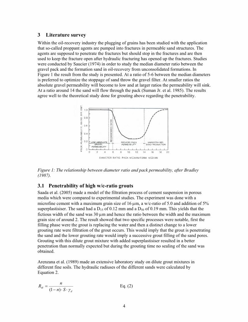
3 Literature survey Within the oil-recovery industry the plugging of grains has been studied with the application that so-called proppant agents are pumped into fractures in permeable sand structures. The agents are supposed to penetrate the fractures but should stop in the fractures and are then used to keep the fracture open after hydraulic fracturing has opened up the fractures. Studies were conducted by Saucier (1974) in order to study the median diameter ratio between the gravel pack and the formation sand in oil-recovery from unconsolidated formations. In Figure 1 the result from the study is presented. At a ratio of 5-6 between the median diameters is preferred to optimize the stoppage of sand throw the gravel filter. At smaller ratios the absolute gravel permeability will become to low and at larger ratios the permeability will sink. At a ratio around 14 the sand will flow through the pack (Suman Jr. et al. 1985). The results agree well to the theoretical study done for grouting above regarding the penetrability.

Figure 1: The relationship between diameter ratio and pack permeability, after Bradley (1987).

3.1 Penetrability of high w/c-ratio grouts Saada et al. (2005) made a model of the filtration process of cement suspension in porous media which were compared to experimental studies. The experiment was done with a microfine cement with a maximum grain size of 16 μm, a w/c-ratio of 5.0 and addition of 5% superplastisiser. The sand had a D15 of 0.12 mm and a D50 of 0.19 mm. This yields that the fictious width of the sand was 30 μm and hence the ratio between the width and the maximum grain size of around 2. The result showed that two specific processes were notable, first the filling phase were the grout is replacing the water and then a distinct change to a lower grouting rate were filtration of the grout occurs. This would imply that the grout is penetrating the sand and the lower grouting rate would imply a successive grout filling of the sand pores. Grouting with this dilute grout mixture with added superplastisiser resulted in a better penetration than normally expected but during the grouting time no sealing of the sand was obtained. Arenzana et al. (1989) made an extensive laboratory study on dilute grout mixtures in different fine soils. The hydraulic radiuses of the different sands were calculated by Equation 2.

dH Sn

nRγ⋅⋅−

=)1(

Eq. (2)

5

According to this equation the calculated hydraulic radiuses were between 2-14 μm. The experiments were done with grouts with a w/c-ratio from 2.0 up to 100 and the d98 of the grout was 10 μm. The findings were that the most important filtration characteristics were the ratio between hydraulic radius and the grain size of cement. Grains larger than one-third of the hydraulic radius was filtered while the smaller grains were filtered in considerable less amounts. For a w/c-ratio of 2 no penetration was possible but the grout penetrated at higher w/c-ratios. From this can it be concluded that the w/c-ratio affects the penetrability. Mittag and Savidis (2003) made experiment where a microfine grout was injected into an injection funnel and hence obtaining a spherical penetration. The grout that was used had a maximum grain size of around 16 μm and the w/c-ratio was 5.0. The sand had a fictious width according to Bergman (1970) of 32 μm implying a ratio of 2 between the aperture and the grout grains. The soil grouting ratio, D15/d85-ratio, between the soil and the grout was around 25. The filtration of the cement was measured by heating samples of the cemented sand and measuring the ignition loss. The result showed that the cement was concentrated in the first half of the penetration radius. This means that most of the cement grains were filtered in the beginning and it was a very thin mixture that was transported through the whole funnel. This is also confirmed by both the rock and soil grouting ratios, which was close to what is considered as groutable.

3.2 Sealing efficiency of high w/c-ratio cement Dupla et al. (2005) made grouting experiments with high w/c-ratio grouts into sand columns. The sand columns were 1040 mm long and had a diameter of 80 mm. The grouts had a w/c-ratio of 5.0 or 10.0. The cements that were used were Spinor A12 and A6, two microfine grouts with grain size less than 12 respectively 6 μm (Microcementos Spinor). The D50 of the sand was 0.19 mm, which yields a fictious width of 30 μm. After grouting, the compression strength of the sand column was tested at five different heights in the column. In Figure 2 an example of the result is presented. In the figure is C2F the same as Spinor A12 and C3F is Spinor A6. C/E stands for the cement/water ratio by weight, which means that the w/c-ratio is the inverse of this value.

Figure 2. Result of the compressive strength at different distances from the grout inlet in a sand column grouted with microfine cement. The term C2F is a grout with a maximum grain size of 12 μm and C3F has a maximum grain size of 6 μm. The two curves to the right have a w/c-ratio of 5.0 and the curve to the left has a w/c-ratio of 10.0. From Dupla et al. (2005). In Figure 2 the distance from the grout inlet is plotted on the y-axis versus the compressive strength on the x-axis (Dupla et al. 2005). The compressive strength of the grouted sand can

6

be seen as an indicator of the amount of deposited cement at the specific penetration length. The ratio between the fictious aperture and the largest grains were 2.5 and 5 for the two cements, respectively. The curve to the right has a maximum grain size of 12 μm and the w/c-ratio was 5.0. As the compressive strength of the grouted column decreases with the distance from the grouting inlet, this would mean that a filtration of the grout occurs. The other two curves also have a decrease in strength from the grouting inlet; however it is not as obvious. The explanation for the results can be:

− At a maximum grain size of 12 μm and a w/c-ratio of 5 (the right curve) is a more obvious filtration occurring compared to the same grout with a w/c-ratio of 10.0 (left curve). This would indicate that at a w/c-ratio of 10.0 is the cement grains more diluted and have a better penetration. In the beginning of the column there is some filtration but from around 30 cm from the grout inlet the grains are deposits in the sand rather uniformly.

− The strength (the amount of deposited cement grains) is less for the cement with a maximum grain size of 6 μm (middle curve) compared to the cement with 12 μm, for the same w/c-ratio. This could either be due to an initial filtration depending on that the small grains are clogging or if the mixing has been really good the reason can be that no larger deposition occurs and the cement passes through the column.

− It can also be concluded that a higher w/c-ratio results in a lower strength of the grouted sand. This seems reasonable since a smaller amount of cement is injected within the same volume of grout.

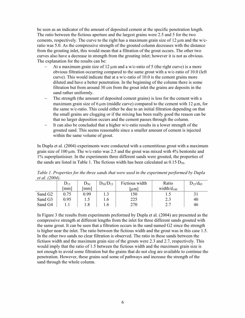
In Dupla et al. (2004) experiments were conducted with a cementitious grout with a maximum grain size of 100 μm. The w/c-ratio was 2.5 and the grout was mixed with 4% bentonite and 1% superplastisiser. In the experiments three different sands were grouted, the properties of the sands are listed in Table 1. The fictious width has been calculated as 0.15⋅D50. Table 1. Properties for the three sands that were used in the experiment performed by Dupla et al. (2004). D15

[mm] D50

[mm] D50/D15 Fictious width

[μm] Ratio

width/d100

D15/d85

Sand G2 0.75 0.99 1.3 150 1.5 31 Sand G3 0.95 1.5 1.6 225 2.3 40 Sand G4 1.1 1.8 1.6 270 2.7 46 In Figure 3 the results from experiments preformed by Dupla et al. (2004) are presented as the compressive strength at different lengths from the inlet for three different sands grouted with the same grout. It can be seen that a filtration occurs in the sand named G2 since the strength is higher near the inlet. The ratio between the fictious width and the grout was in this case 1.5. In the other two sands no clear filtration is observed. The ratio in these sands between the fictiuos width and the maximum grain size of the grouts were 2.3 and 2.7, respectively. This would imply that the ratio of 1.5 between the fictious width and the maximum grain size is not enough to avoid some filtration but the grains that do not clog are available to continue the penetration. However, these grains seal some of pathways and increase the strength of the sand through the whole column.

7

Figure 3. The compressive strength at different lengths from the grout inlet in three different sands grouted with a grout with maximum grain size of 100 μm and a w/c-ratio of 2.5. After Dupla et al. (2004). Sanatagata and Santagata (2003) conducted sand column experiments with a microcement that had a maximum grain size of around 12 μm. The experiments were made with a w/c-ratio ranging from 1.5 to 5.0 and different amounts of superplastisiser and grouting pressure were used. Three different sands were used, which are described in Table 2. The fictious width has been calculated as 0.15⋅D50. Table 2. Properties for the three sands that were used in the experiment performed by Sanatagata and Santagata (2003). D15

[mm] D50

[mm] D50/D15 Fictious width

[μm] Ratio

width/d100 D15/d85

Ticino 0.35 0.55 1.6 82 6.9 78 Basaltic 0.30 1.0 3.3 150 12.5 67 Siliceous-calcareous

0.22

1.2

5.5

180

15.0

49

As can be seen in Table 2 the ratio between the sand and the grain sizes in the grout are so large that penetration would be possible even for low w/c-ratios. It should also be noted that the two last sands in Table 2 have a larger amount of fines than the first one. This is the explanation for that the ratio between fictious width and d100 of the grout is increasing while the ratio between D15 of the sand and the d85 of the grout is decreasing from the top of Table 2 and down. In Figure 4 the results of some of the experiments made by Sanatgata and Santagata (2003) are presented as the penetration length of different w/c-ratios in the different sands. In the Ticino sand a quite linear relationship is obtained between w/c-ratio and penetrability. But for the other two sands no increases in penetrability are shown for experiments over a w/c-ratio of around 3.5. The authors explain this phenomenon as a separation of the cement and the water. It can also be considered as a plugging of the flow paths with cement grains. There was no compression test or other evaluation done of the amount of cement that was plugged so the sealing efficiency is difficult to estimate. The explanation of why this does not occur in all three sands could be that the two sand where it does occur have larger amount of fines.

8

Figure 4. The penetration length for different w/c-ratios in three sands. After Sanatagata and Sanatagata (2003). Zebovitz et al. (1989) made experiments with a grout that had a maximum grain size of 15 μm. Three different w/c-ratios were used, w/c-ratio of 2, 4 and 6. The grouts were injected into sand columns where three different sands were used. In Table 3 the properties of the sands are presented, with use of the assumption that the fictious width is calculated with 0.15⋅D50. Table 3. Properties for the three sands that were used in the experiment performed by Zebovitz et al. (1989). D15

[mm] D50

[mm] D50/D15 Fictious

width [μm]

Ratio width/d100

D15/d85 Eff. permeability

[m/s] Evanston Beach

0.17 0.23 1.4 38 2.5 28 1.8⋅10-4

Torpedo I 0.22 0.45 2.0 68 4.5 37 2.3⋅10-4 Torpedo II 0.43 1.4 3.3 180 12.0 72 1.9⋅10-4 In Figure 5 the results from the experiments made by Zebovitz et al. (1989) are presented as permeability (diagram a, c and e) and the compressive strength (diagram b, d and f) at different distances from the injection point. It can be noticed that the compressive strength for a w/c-ratio of 2 decreases with increased distance from the injection point as well as the permeability increases from the injection point. This is not so obvious for the w/c-ratios of 4 and 6. This would indicate that the filtration of cement is more efficient for a w/c-ratio of 2. At a w/c-ratio of 6 there is almost no difference in the compressive strength while for a w/c-ratio of 2 a large difference can be noticed between near the inlet and near the outlet of the column. The authors could not identify any apparent reason explaining that the compressive strength is higher for the second measured value compared to the first measured value at a couple of measuring series. To conclude the findings in the experiments:

− At a w/c-ratio of 2 there is an obvious decrease in permeability obtained through the whole sand column in all experiments. Some filtration occurs and more cement grains deposits near the grout inlet.

− At a w/c-ratio of 6 the effect on the permeability is low. However, in the sand with the narrowest fictious width the effect is most obvious. This would indicate that the grains are more likely to settle in smaller pathways than in larger.

9

− For the experiments with a w/c-ratio of 4 the effect is similar to the results for the experiments done with a w/c-ratio of 6. In the sand with the narrowest fictious width the sealing efficiency is most obvious.

Figure 5. The permeability and the compressive strength for three different sands grouted with the same cement but with different w/c-ratios. After Zebovitz et al. (1989).

3.3 Conclusions regarding the literature survey In order to achieve a penetration of a particle suspension such as cementitious grouts, several authors seems to come to the conclusion that the maximum particle size of the suspension has to be maximum one-third of the aperture. Otherwise is it likely that plugging occurs and the suspension will be filtrated. The experiments that have been studied in the literature survey show that it is possible to penetrate finer widths with higher w/c-ratios. However, it seems like some filtration occurs during the penetration and most cement grains are stopped closer to the grouting inlet. The cement grains that are not filtered near the inlet can however continue the penetration further and stop at longer distances from the grouting inlet. The effect of the deposition of cement grains in the sand have been measured as an increase in the sand strength in most of the experiments. Most experiments show that a filtration effect occurs and the largest strengths of the sands are near the grout inlet. The filtration effect is often shown to decrease as the w/c-ratio increases. The effect of using finer maximum grain size of the cement seems to result in a lower strength of the sand. This can depend on a better penetration but also it can be a matter of initial clogging of the cement grains if a proper grout mixing is not done. In the only experiment that also has evaluated the permeability, it seems as the permeability is reduced for a w/c-ratio of 2. However, as the w/c-ratio is increased, the effect is more limited but in the sand with the narrowest fictious width there is also a reduction in permeability for a w/c-ratio of 6.

10

4 Theory behind filtration In the literature study a number of experiments have shown that a filtration process occurs as the w/c-ratio increases. This part is done in order to do a theoretical explanation of the filtration process as the cement particles plug the path between the sand grains. The penetration of small grains through larger grains in something that has been investigated in the design of sand filters for wells. According to Andersson et al. (1984), the ratio should be in the range of 2.4-6.5 between the gravel pack and the formation. This is based on the theoretical consideration of the packing of spherical grains. By using geometrical relationships, the ratio between the grains that just will pass through the different extreme degrees of packing can be determined, see Figure 6.

Figure 6: The largest grain that can pass through a pore system. To the left, dense packed grains and to the right loose packed material. The hypotenuses of the small triangles are in both cases R+r, where R is radius of the large grains and r is the radius of the small grains. In Figure 6 a triangle is sketched in both figures in which the hypotenuse is R+r, where R is the radius of the large grain and r is the radius of the small grain. For the dense packed material the filter grains can be seen as a triangle that allows the passing grain through in the middle. The sketched triangle to the left figure in Figure 6 will have the angles of 30, 60 and 90°. This means that the sides are R and R/2 respectively and the hypotenuse can be written as:

Rh3

2= . Eq. (3)

This means that there are two expressions for the hypotenuse and these can be combined:

RrR3

2=+ . Eq. (4)

If this expression is developed the ratio between the grains can be expressed as:

5.61

32

1≈

−=

rR . Eq. (5)

For the loose packed material to the right in Figure 6, the triangle will have angles of 45, 45 and 90°. This means that the length of two of the sides R and the hypotenuse can be expressed as:

R R r

r

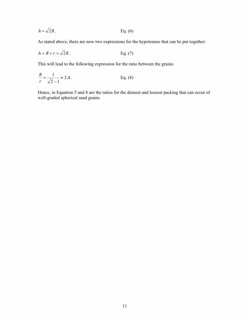
11

Rh 2= . Eq. (6) As stated above, there are now two expressions for the hypotenuse that can be put together:

RrRh 2=+= . Eq. (7) This will lead to the following expression for the ratio between the grains:

4.212

1≈

−=

rR . Eq. (8)

Hence, in Equation 5 and 8 are the ratios for the densest and loosest packing that can occur of well-graded spherical sand grains.

12

5 Laboratory experiments in sand column In order to corroborate the findings presented in the literature survey, laboratory experiments were performed. The experiments were done in a water saturated sand column that was grouted with a Bingham fluid. The height of the column was 1 meter and the sand was filled up to a height of 0.9 meters. The diameter of the column was 9.9 centimetres. In the top and the bottom of the column were filters placed. The sand column was water saturated with de-aired water that was filled from the bottom. Both the conductivity measurements and the grouting were performed from the top of the column. In order to determine the penetrability and sealing mechanism, different water saturated sands were grouted by a Bingham fluid with different w/s-ratios (water/solid-ratios).

5.1 Method The methodology of the sand column is described in detail by Funehag (2005). Briefly, the set-up consists of three containers; a grout container, a sand column and a water column. Every test followed the same methodology, which were done in the following order:

1. Filling of sand in a column 2. Weighting of column 3. Water saturation of the column with de-aired water 4. Weighting of column 5. Hydraulic conductivity measurement of the sand. By measuring the water flow

through the column and the pressure distribution along the column at constant water pressure, the hydraulic conductivity is determined.

6. Grouting of the sand from pressurised grouting tank. The penetration is measured in a water tank after the sand column and as the grout take in the grout tank. Grouting is conducted with 2.6 bars over pressure.

The experimental set-up of the sand column is presented in Figure 7.

Figure 7. Layout of the sand column.

Piezometers

Sand

Filter

Water container with adjustable height

Water container with adjustable height

De-aeration valves

Valve

Pressure, P1

Pressure, P2

ValveQ(K)

Δh Measuring scale

Container for grout

Reduction valve

Reduction valve

Filter stone

I

13

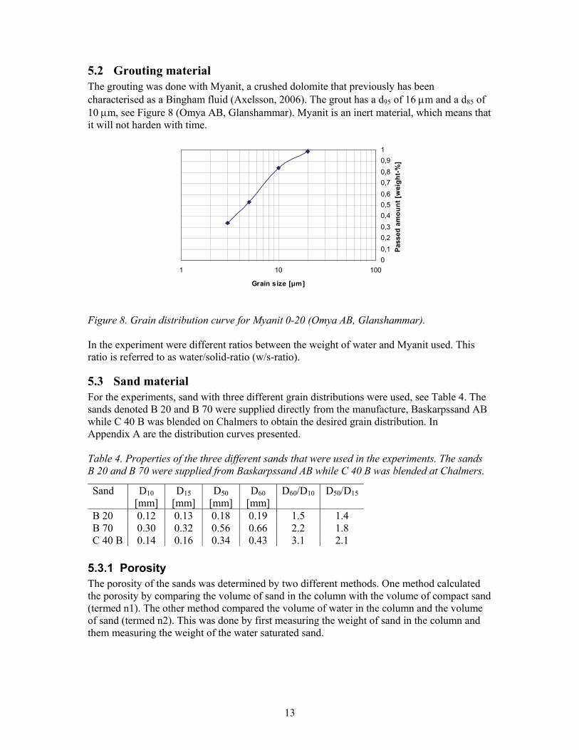
5.2 Grouting material The grouting was done with Myanit, a crushed dolomite that previously has been characterised as a Bingham fluid (Axelsson, 2006). The grout has a d95 of 16 μm and a d85 of 10 μm, see Figure 8 (Omya AB, Glanshammar). Myanit is an inert material, which means that it will not harden with time.

Figure 8. Grain distribution curve for Myanit 0-20 (Omya AB, Glanshammar). In the experiment were different ratios between the weight of water and Myanit used. This ratio is referred to as water/solid-ratio (w/s-ratio).

5.3 Sand material For the experiments, sand with three different grain distributions were used, see Table 4. The sands denoted B 20 and B 70 were supplied directly from the manufacture, Baskarpssand AB while C 40 B was blended on Chalmers to obtain the desired grain distribution. In Appendix A are the distribution curves presented. Table 4. Properties of the three different sands that were used in the experiments. The sands B 20 and B 70 were supplied from Baskarpssand AB while C 40 B was blended at Chalmers.

5.3.1 Porosity The porosity of the sands was determined by two different methods. One method calculated the porosity by comparing the volume of sand in the column with the volume of compact sand (termed n1). The other method compared the volume of water in the column and the volume of sand (termed n2). This was done by first measuring the weight of sand in the column and them measuring the weight of the water saturated sand.

Sand D10 [mm]

D15 [mm]

D50 [mm]

D60 [mm]

D60/D10 D50/D15

B 20 0.12 0.13 0.18 0.19 1.5 1.4 B 70 0.30 0.32 0.56 0.66 2.2 1.8 C 40 B 0.14 0.16 0.34 0.43 3.1 2.1

00,10,20,30,40,50,60,70,80,91

1 10 100

Grain size [μm]

Pass

ed a

mou

nt [w

eigh

t-%

]

14

5.3.2 Specific surface The specific surface can be determined either from the grain distribution curve or from hydraulic measurements of the sand (Gustafson 1983). The traditional method to determine the specific surface from grain distribution curves is to calculate the specific surface for each sieving fraction according to Equation 9. The term α is considering the shape of the grains and for spherical grains, the factor is 6.

⎟⎟⎠

⎞⎜⎜⎝

⎛−

⎟⎟⎠

⎞⎜⎜⎝

⎛

−=

++

++−+−

)1()1(

)1()1()1(,

11

ln

)(

nn

n

n

nnnnnnS dd

dd

ppS

α Eq. (9)

However, in Appendix B is a simplified expression developed to determine the specific surface from the grain distribution curve. The expression only considers D60 and D10 of the grain distribution curve, see Equation 10.

)ln21.0ln84.0(ln 2106 UUDeS ++−= Eq. (10)

U is determined by:

10

60

DD

U = . Eq. (11).

It is also possible to determine the specific surface from the hydraulic conductivity measurements that are conducted in the sands. The advantage of this method is that it is considering the porosity and the permeability of the sand, which can differ depending on the packing of the sand. This is not considered in the methods from the grain distributions curve. Roughly, it can be stated that the specific surface from the hydraulic measurements are considering the available specific surface whereas the specific surface from the grain distribution curve yields the theoretical surface. In Equation 12 the relationship for the specific surface determined from hydraulic measurements is presented. The equation is a rearrangement of the Kozeny-Carman equation (Carman 1937).

( ) knnCS CK

11 2

3

3 ⋅−

=− Eq. (12)

5.3.3 Aperture The penetrability for a Newtonian fluid such as water and a suspension such as a Bingham fluid differs. As stated above, the grains in the suspension cannot enter all of the space that a Newtonian fluid can. This also means that the available space in the sand column that can be filled with water is not the same as the space that can be filled with the grout. Consequently, the measured porosity and permeability, which is done with water, is not a representative measurement for the available volume for a suspension grout, see Figure 9. The shaded area to right in the figure represents the area available for a suspension (Bingham fluid) whereas closer to the contact point between the grains, only water (Newtonian fluid) will be able to penetrate.

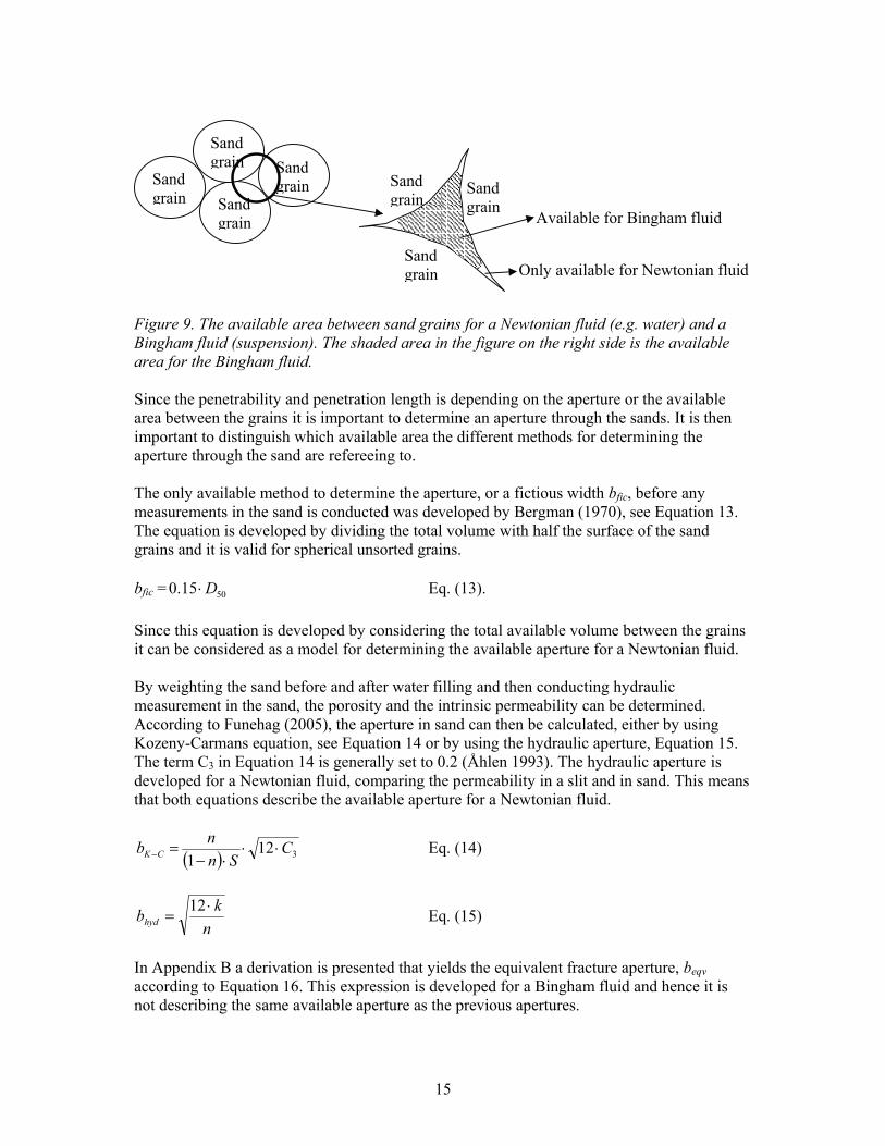
15

Figure 9. The available area between sand grains for a Newtonian fluid (e.g. water) and a Bingham fluid (suspension). The shaded area in the figure on the right side is the available area for the Bingham fluid. Since the penetrability and penetration length is depending on the aperture or the available area between the grains it is important to determine an aperture through the sands. It is then important to distinguish which available area the different methods for determining the aperture through the sand are refereeing to. The only available method to determine the aperture, or a fictious width bfic, before any measurements in the sand is conducted was developed by Bergman (1970), see Equation 13. The equation is developed by dividing the total volume with half the surface of the sand grains and it is valid for spherical unsorted grains. bfic = 5015.0 D⋅ Eq. (13). Since this equation is developed by considering the total available volume between the grains it can be considered as a model for determining the available aperture for a Newtonian fluid. By weighting the sand before and after water filling and then conducting hydraulic measurement in the sand, the porosity and the intrinsic permeability can be determined. According to Funehag (2005), the aperture in sand can then be calculated, either by using Kozeny-Carmans equation, see Equation 14 or by using the hydraulic aperture, Equation 15. The term C3 in Equation 14 is generally set to 0.2 (Åhlen 1993). The hydraulic aperture is developed for a Newtonian fluid, comparing the permeability in a slit and in sand. This means that both equations describe the available aperture for a Newtonian fluid.

( ) 3121

CSn

nb CK ⋅⋅⋅−

=− Eq. (14)

nkbhyd⋅

=12 Eq. (15)

In Appendix B a derivation is presented that yields the equivalent fracture aperture, beqv according to Equation 16. This expression is developed for a Bingham fluid and hence it is not describing the same available aperture as the previous apertures.

Sand grain

Sand grain

Sand grain

Sand grain

Only available for Newtonian fluid Sand grain

Available for Bingham fluid

Sandgrain

Sand grain

16

Snbeqv ⋅−⋅

=)1(

8π

. Eq. (16)

As stated earlier, the penetrability of a Newtonian fluid is in the range of 3-5 times better than for a Bingham fluid, such as suspensions. This means that beqv should be in the range of 3-5 times larger than the apertures developed for Newtonian fluids (bK-C and bhyd). The rule of thumb for soil grouting, stated earlier, describes the possibility of penetration and hence is a measurement connected to the characteristic of the grout. For a suspension, this implies that it is considering the available area for the Bingham fluid, see Figure 9. However, the rule of thumb for the rock is based on measurement of the hydraulic aperture, which considering the whole area in Figure 9 and hence the availability of a Newtonian fluid. In Table 5 the parameters for determine the aperture and the rules of thumb for grouting are summarised. The parameters assume that grouting will be performed by a suspension (Bingham fluid). Table 5. Summary of the different parameters for determining the penetrability from available space considering grouting with a suspension (Bingham fluid) and hydraulic measurement with water (Newtonian fluid). Parameter Rheological model bfic Newtonian bK-C Newtonian bhyd Newtonian beqv Bingham

2585

15 >Grout

Soil

dD

Bingham

b>3-5⋅d95 Newtonian In Table 6, the characteristics of the different sands that were determined on the basis of the sand and grout distribution curves are presented. In order to compare the ratios a d95 of 16 μm for the grout has been used and to calculate the rock fracture ratio has the fictious aperture (bfic) been used.

17

Table 6. The widths in the three different sands and the rule of thumbs for soil and rock grouting assuming a grout with d95 of 16 μm. The rock fracture rule of thumb is calculated by using the fictious width of the sand. Sand bfic

[μm] Soil grouting ratio

Rock fracture ratio

B 20 27 13 1.7 B 70 84 32 5.3 C 40 B 51 16 3.2

5.4 Hypothesis The penetrability and sealing mechanism is evaluated by using sand material with different apertures between the grains and the same grout but with different w/s-ratios. The properties of the sand are described by the relationships stated above and the properties of the grout are related to the grain distribution curve. Hence, the hypothesis is that the penetration will stop due to three different processes:

– The grout does not penetrate. This is due to that the suspension grains are larger than one-third of the aperture between the grains.

– The suspension grains penetrate more or less “one by one” and successively block the pathways. This occurs in suspension mixtures with high w/s-ratios.

– The grout penetrates and stops due to that the acting grout pressure does not exceed the resisting force in the material.

In order to test these hypotheses, four different experiments were set-up.

1. Using sand B 20 and the grout was mixed with a w/s-ratio of 3.0. As seen in Table 5, this should imply that no penetration is expected due to the narrow passages between the sand grains (soil grouting ratio of 13 and rock grouting ratio of 1.7).

2. Using sand C 40 M and w/s-ratio of 1.0. According to Table 5 this would be close to the limit for what is possible to penetrate. The soil grouting ratio (16) is less than what is considered as groutable whereas the rock grouting ratio is close to the limit (3.2).

3. Using sand C 40 M but with a w/s-ratio of 3.0 instead. The hypothesis is that single grout particles are able to penetrate the sand but not the entire grout suspension.

4. Using sand B 70 and a w/s-ratio of 1.0. Both the soil grouting ratio and the rock grouting ratio indicates that the grout will be able to penetrate this sand as a suspension. Stoppage should occur due to the friction towards the sand grains.

The maximum penetration for a Bingham fluid can be calculated as (Gustafson and Stille, 1995):

0max 2τ

bpI ⋅Δ= Eq. (17)

The grouting time was set to 30 min. This implies that the grout would penetrate through the whole column for the B 70 sand. By using the analytic solution to the penetration developed by Gustafson and Claesson (2006) it was shown that it only should take 4-5 minutes to penetrate the whole column in the B 70 sand. However, in order to have sufficient grouting time to be able to see the processes that was expected and since the same grouting time was desired for all experiments in order to have similar test conditions, a grouting time of 30 minutes was chosen.

18

To determine the penetration of the grout, three different measurements were conducted:

− The increase of water in the water tank after the sand column. − The decrease of grout in the grout column. − Visual measurement during emptying of the sand from the column. It was not

possible to detect absolute limits of the penetration but it was possible to see a gradual decrease of grout in the sand.

19

6 Results In this chapter the evaluation of the sand properties and the measured penetration in the sand column are presented.

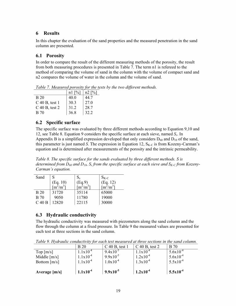
6.1 Porosity In order to compare the result of the different measuring methods of the porosity, the result from both measuring procedures is presented in Table 7. The term n1 is refereed to the method of comparing the volume of sand in the column with the volume of compact sand and n2 compares the volume of water in the column and the volume of sand. Table 7. Measured porosity for the tests by the two different methods. n1 [%] n2 [%] B 20 40.0 44.7 C 40 B, test 1 30.3 27.0 C 40 B, test 2 31.2 28.7 B 70 36.8 32.2

6.2 Specific surface The specific surface was evaluated by three different methods according to Equation 9,10 and 12, see Table 8. Equation 9 considers the specific surface at each sieve, named Ss. In Appendix B is a simplified expression developed that only considers D60 and D10 of the sand, this parameter is just named S. The expression in Equation 12, SK-C is from Kozeny-Carman’s equation and is determined after measurements of the porosity and the intrinsic permeability. Table 8. The specific surface for the sands evaluated by three different methods. S is determined from D60 and D10, Ss from the specific surface at each sieve and SK-C from Kozeny-Carman’s equation.

6.3 Hydraulic conductivity The hydraulic conductivity was measured with piezometers along the sand column and the flow through the column at a fixed pressure. In Table 9 the measured values are presented for each test at three sections in the sand column. Table 9. Hydraulic conductivity for each test measured at three sections in the sand column. B 20 C 40 B, test 1 C 40 B, test 2 B 70 Top [m/s] 1.1x10-4 9.4x10-5 1.1x10-4 5.6x10-4 Middle [m/s] 1.1x10-4 9.9x10-5 1.2x10-4 5.6x10-4 Bottom [m/s] 1.1x10-4 1.0x10-4 1.3x10-4 5.5x10-4 Average [m/s] 1.1x10-4 9.9x10-5 1.2x10-4 5.5x10-4

Sand S (Eq. 10) [m2/m3]

Ss (Eq.9) [m2/m3]

SK-C (Eq. 12) [m2/m3]

B 20 31720 35114 65000 B 70 9050 11780 19000 C 40 B 12820 22115 30000

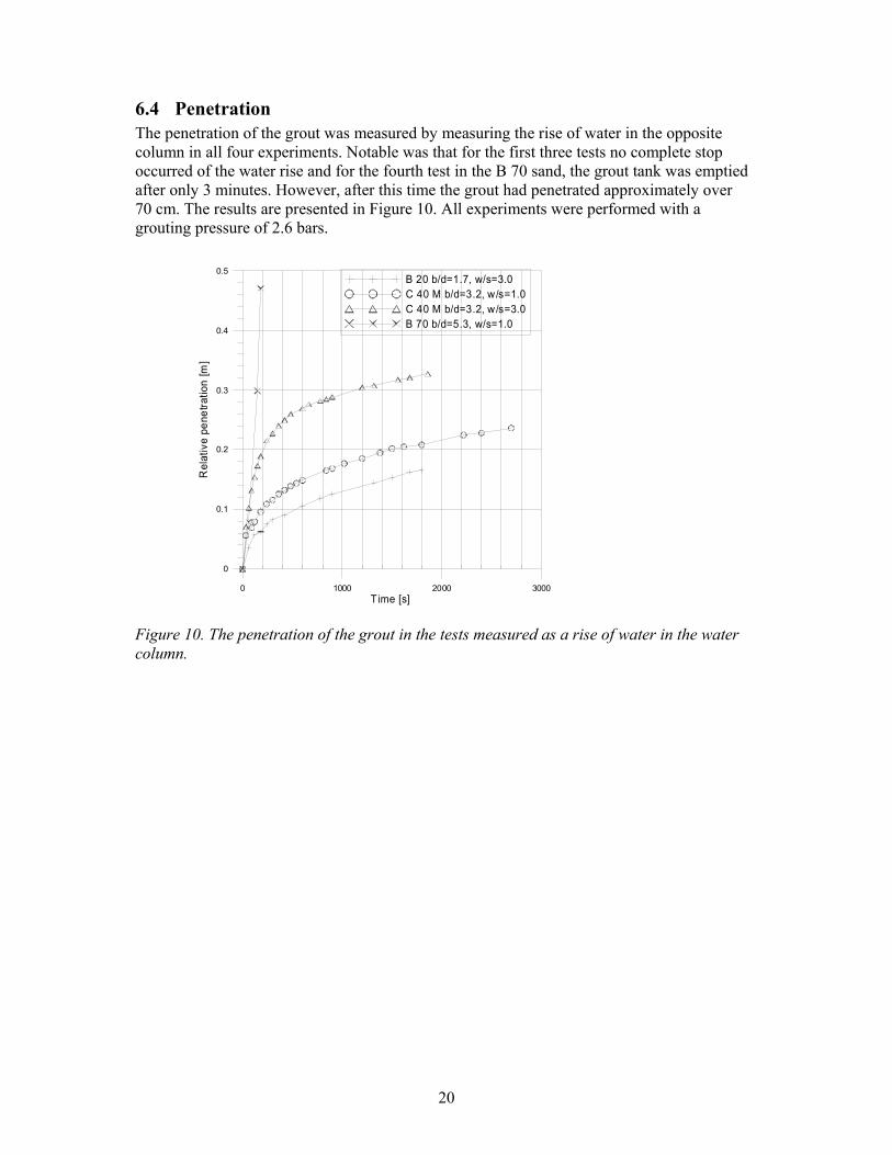
20

6.4 Penetration The penetration of the grout was measured by measuring the rise of water in the opposite column in all four experiments. Notable was that for the first three tests no complete stop occurred of the water rise and for the fourth test in the B 70 sand, the grout tank was emptied after only 3 minutes. However, after this time the grout had penetrated approximately over 70 cm. The results are presented in Figure 10. All experiments were performed with a grouting pressure of 2.6 bars.

Figure 10. The penetration of the grout in the tests measured as a rise of water in the water column.

0 1000 2000 3000Time [s]

0

0.1

0.2

0.3

0.4

0.5

Rel

ativ

e pe

netra

tion

[m]

B 20 b/d=1.7, w/s=3.0C 40 M b/d=3.2, w/s=1.0C 40 M b/d=3.2, w/s=3.0B 70 b/d=5.3, w/s=1.0

21

7 Discussion

7.1 Porosity The porosity was determined by two different methods, either by comparing the volume of sand in the column with the volume of compact sand or by comparing the volume of water in the column and the volume of sand. As can be seen in Table 7, the difference between the methods is in the range of 10% and this is probably an indication of measuring accuracy of the porosity.

7.2 Specific surface The specific surface was determined by three different methods according to Table 8. The simplified method developed in Appendix B that determines the specific surface from the D60 and the D10 of the sand seems to yield reasonable values for B 20 and B 70 sands. The difference is in the range of 10-15%. For the C 40 B sand the values are differing more, around 40%. This could be explained by the fact that the latter sand has a wider grain distribution curve and the error of simplifying the curve with just two points is increasing. The specific surface determined by the Kozeny-Carman equation, SK-C is generally almost twice as large compared to the other methods. This emphasis the difficulties of determining the specific surface of a material but it should also be noted that the method of using Kozeny-Carman is evaluating the porosity of the sand in cubic, which means that this parameter is very sensitive. It should also be noted that SK-C is based on hydraulic measurement whereas the other methods are based on the grain size distribution curve.

7.3 Hydraulic conductivity By studying Table 9, it can be noticed that the hydraulic conductivity does not differ particularly through the length of the sand column. Since the weight of the overburden sand could imply denser sand in the bottom compared to the upper part of column, it could be expected that the hydraulic conductivity would be lower at the bottom. However, observations showed that the upper centimetres were more permeable and some penetration into this area occurred in all tests. The hydraulic conductivity was similar in the first three tests although the theoretical width should be larger for C 40 B. However, the porosity was much lower in C 40 B compared with C 20, which could indicate that the more unsorted C 40 B sand implied denser sand. This also means that the equation for fictious width is more uncertain since it is just based on one value on the grain distribution curve, the D50 of the sand.

7.4 Penetration Since grouting was performed with suspension grout, it could be expected that a grout plug or filter cake is formed. As can be seen in Figure 10, all the penetration curves are bending after some time. This is probably a measurement of the forming of a filter cake by compaction / separation effects of the grout in the upper part of the sand column combined with possible water drainage in the lower part of the sand column. In the piezometric pipes in the sand column, there was no measurable pressure. This means that the whole pressure is distributed over the filter cake. The main part of the penetration generally occurred during the first 5-10 minutes; see Figure 8, after which the rate of penetration successively decreases. During this first time, the penetration curve is rather linear. The last part of the water penetration curves shows a more or less constant flow and the flow is around the same magnitude in all the tests.

22

Visually it was difficult to see any further penetration after this time and hence the actual penetration should be determined at the bend of the penetration curve. In Appendix D an expression between the penetration and the time for a filter cake is developed. The expression shows that as a filter cake is formed, the penetration is proportional to the square of time. In Figure 11 the penetration are plotted against the square of time. The filled lines do all have the same inclination and hence describes the same process whereas the dotted lines have different inclinations. Since the penetration should be proportional to the square of the time but with different inclinations, the lines in Figure 11 indicates that there is an initial penetration followed by a growth of a filter and as the inclination becomes constant, there have been a filter cake formed stopping further penetration. It should be noted that the penetration in Figure 11 corresponds well to the penetration visually detected in the sand column during emptying.

Figure 11. The penetration versus the square of the time. The dotted lines indicates the penetration and the filled lines, which all have the same inclination, shows the forming of a filter cake. Measurement of the penetration was conducted by two different methods during grouting, the lowering in the grout column before the sand column and the rise of water in the water column after the sand column. In Figure 12 the result from these two measurements are presented for two of the experiments. Reading of the grout level was only possible for the experiments performed with a w/s-ratio of 3.0. In the experiments with a w/s-ratio of 1.0 the grout was attaching to the measuring pipe on the grout tank and made reading impossible. The difference between the measuring places is limited for the B 20 sand whereas there is a larger difference for the C 40 B sand. In the latter case, the fact that the grout penetration

0 20 40 60 80 100Time2 [s2]

0

0.1

0.2

0.3

0.4

0.5

Rel

ativ

e pe

netra

tion

[m]

B 20 b/d=1.7, w/s=3.0C 40 M b/d=3.2, w/s=1.0C 40 M b/d=3.2, w/s=3.0B 70 b/d=5.3, w/s=1.0

23

exceeds the measured penetration after the sand column indicates that the grout is filtered/compacted in the upper part of the sand column.

Figure 12. Comparison between measured penetration by measuring the water rise in the water column after the sand column and grout sink in the grout tank before the sand column.

7.5 Aperture In order evaluate the aperture in the sands the available area depending on rheological model, as presented in Table 5, has to be distinguished. The evaluated apertures are presented in Table 10 where parameters evaluated with Newtonian fluids are to the left and Bingham fluids are to the right. For the parameters evaluated by Newtonian fluid the aperture is rather consistent but the aperture determined from the hydraulic conductivity, bhyd, is generally half of the fictious aperture, bfic, and the aperture determined from the equation of Kozeny-Caraman, bK-C. The method developed in Appendix B, beqv, which is describing an available area for a Bingham fluid, should theoretical be in the range of 3 to 5 times larger than the aperture determined by Newtonian fluid. Comparing the values in Table 10, especially considering bfic and bK-C , with the value of the equivalent aperture, the values seem to be within this range. To evaluate the apertures in Table 10 the expression for the specific surface developed in Appendix B have been used.

0 500 1000 1500 2000 2500 3000 3500 4000Time [s]

0

0.1

0.2

0.3

0.4

0.5

0.6

Pene

tratio

n [m

]Grout penetration, B 20 w/s=3.0Water penetration, B 20 w/s=3.0Grout penetration, C 40 B w/s=3.0

Water penetration, C 40 B w/s=3.0

24

Table 10. The widths in the three different sands and the rule of thumbs for soil and rock grouting assuming a grout with d95 of 16 μm. To the left are parameters determined by Newtonian fluids and to the right parameters determined by Bingham fluids. Sand bfic

[μm] bK-C

[μm] bhyd

[μm] Rock fracture

ratio beqv

[μm] Soil grouting

ratio B 20 27 40 18 1.7 63 13 B 70 84 81 45 5.3 230 32 C 40 B 51 47 24 3.2 135 16

7.6 Mixing The mixing of the grout was done manually through stirring the grout. This could imply that the actual grain size of the grout could be larger than calculated due to some clogging during mixing. This was also observed at the bottom of the mixing bucket after the grout has been poured into the grouting tank.

7.7 Experiments The four experiments can be summarised as:

• Experiment 1, B 20 and w/s-ratio of 3.0. The hypothesis was that grout should not be able to penetrate. This was principally confirmed in the experiments, although the penetration was a couple of centimetres and it occurred immediately after the grouting started. The reason for this was probably due to that the sand was less packed in the upper part. The measured penetration in the water column (just over 20 cm) and in the grout column (around 24 cm) was larger than the visual determined penetration during emptying of the sand. However, the linear part of the penetration curve indicates a penetration of 2-8 cm, which is closed to the visual determined.

• Experiment 2, C 40 B and w/s-ratio of 1.0. The hypothesis was that limited penetration

should occur. Measured penetration in the water column was around 25 cm but the linear part of the penetration curve was just around 12 cm. The visual examination indicated a penetration of around 3 cm and then a successive decrease in grout down to around 10 cm.

• Experiment 3, C 40 B and w/s-ratio of 3.0. The hypothesis was that limited penetration

should occur but single grains should be transported further and successively block the pathways. Measured penetration in the water column was 35 cm and in the grout column 55 cm. The linear parts of the curves indicate a penetration of 25-35 cm. During the emptying of the sand it was noticed that the first centimetres were clearly grouted, after around 10 cm it was less grout but still clearly visual and after approximately 30 cm there was no grout in the column.

• Experiment 4, B 70 and w/s-ratio of 1.0. The hypothesis was that the grout should be

able to penetrate this sand. Measured penetration in the water column was around 50 cm. Visual examination showed homogenous grout penetration 40-50 cm and trace of grout to over 70 cm. The experiment was ended because the grout tank was emptied. By using the analytic solution to the penetration developed by Gustafson and Claesson (2006) and back calculate the length of the penetration after 3 minutes, it shows that around 80 cm should be grouted, see also Figure 12.

25

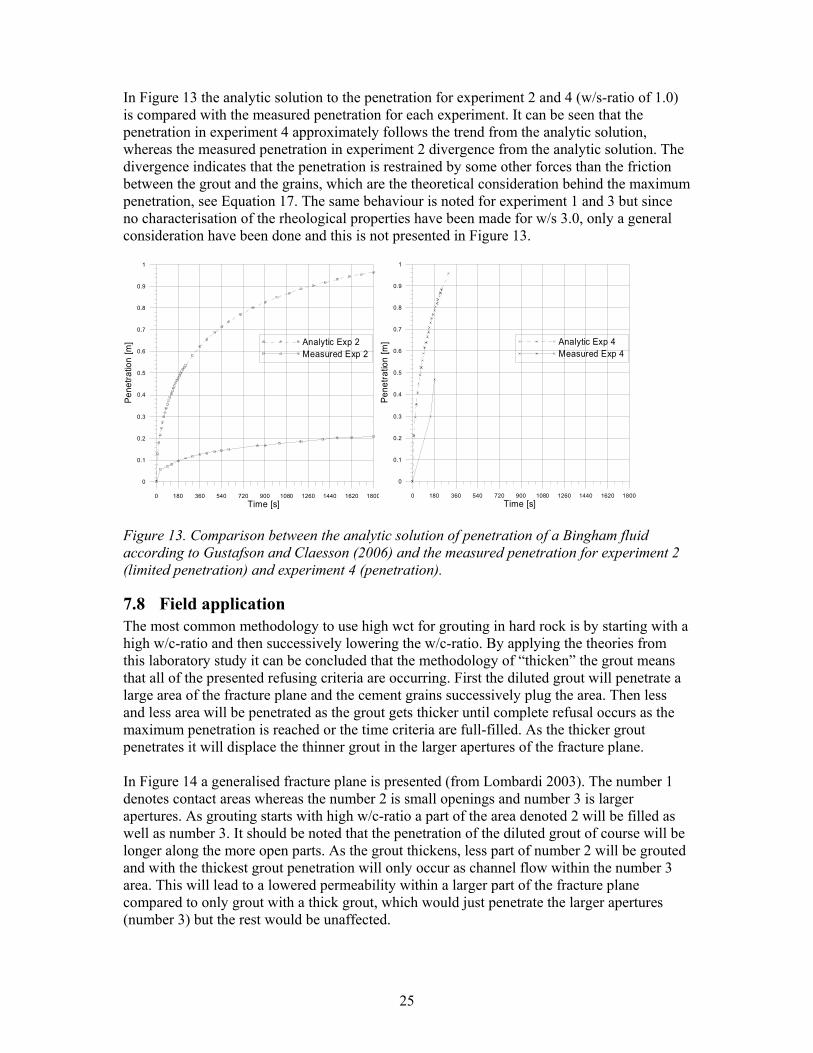
In Figure 13 the analytic solution to the penetration for experiment 2 and 4 (w/s-ratio of 1.0) is compared with the measured penetration for each experiment. It can be seen that the penetration in experiment 4 approximately follows the trend from the analytic solution, whereas the measured penetration in experiment 2 divergence from the analytic solution. The divergence indicates that the penetration is restrained by some other forces than the friction between the grout and the grains, which are the theoretical consideration behind the maximum penetration, see Equation 17. The same behaviour is noted for experiment 1 and 3 but since no characterisation of the rheological properties have been made for w/s 3.0, only a general consideration have been done and this is not presented in Figure 13.

0 180 360 540 720 900 1080 1260 1440 1620 1800Time [s]

0

0.1

0.2

0.3

0.4

0.5

0.6

0.7

0.8

0.9

1

Pene

tratio

n [m

] Analytic Exp 2Measured Exp 2

0 180 360 540 720 900 1080 1260 1440 1620 1800Time [s]

0

0.1

0.2

0.3

0.4

0.5

0.6

0.7

0.8

0.9

1

Pene

tratio

n [m

] Analytic Exp 4Measured Exp 4

Figure 13. Comparison between the analytic solution of penetration of a Bingham fluid according to Gustafson and Claesson (2006) and the measured penetration for experiment 2 (limited penetration) and experiment 4 (penetration).

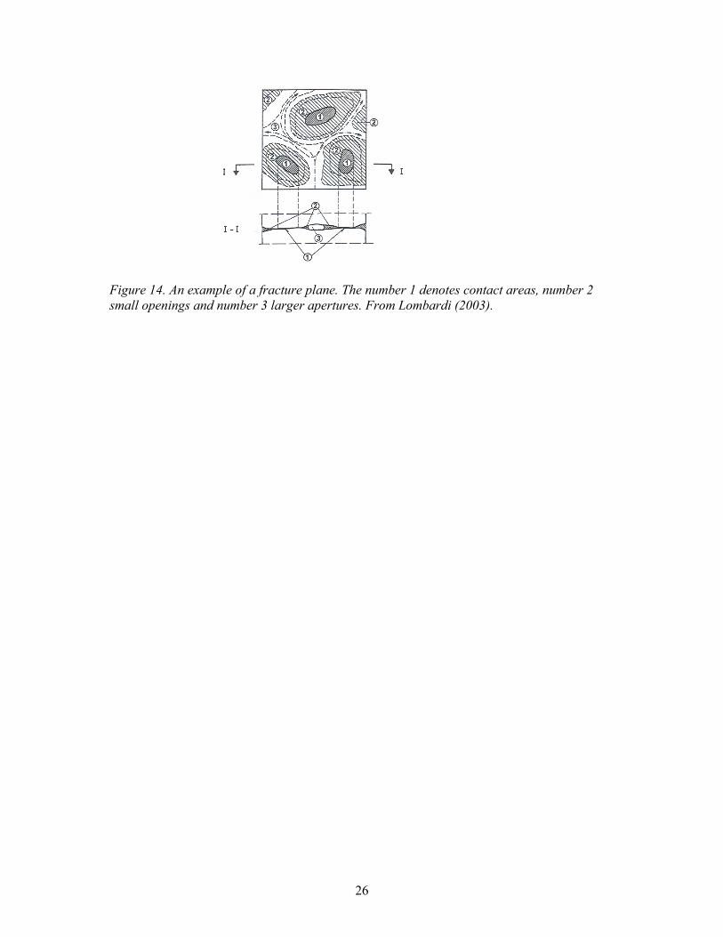
7.8 Field application The most common methodology to use high wct for grouting in hard rock is by starting with a high w/c-ratio and then successively lowering the w/c-ratio. By applying the theories from this laboratory study it can be concluded that the methodology of “thicken” the grout means that all of the presented refusing criteria are occurring. First the diluted grout will penetrate a large area of the fracture plane and the cement grains successively plug the area. Then less and less area will be penetrated as the grout gets thicker until complete refusal occurs as the maximum penetration is reached or the time criteria are full-filled. As the thicker grout penetrates it will displace the thinner grout in the larger apertures of the fracture plane. In Figure 14 a generalised fracture plane is presented (from Lombardi 2003). The number 1 denotes contact areas whereas the number 2 is small openings and number 3 is larger apertures. As grouting starts with high w/c-ratio a part of the area denoted 2 will be filled as well as number 3. It should be noted that the penetration of the diluted grout of course will be longer along the more open parts. As the grout thickens, less part of number 2 will be grouted and with the thickest grout penetration will only occur as channel flow within the number 3 area. This will lead to a lowered permeability within a larger part of the fracture plane compared to only grout with a thick grout, which would just penetrate the larger apertures (number 3) but the rest would be unaffected.

26

Figure 14. An example of a fracture plane. The number 1 denotes contact areas, number 2 small openings and number 3 larger apertures. From Lombardi (2003).

27

8 Conclusions The objective of this study was to develop theory for stop mechanisms from literature survey and theoretical studies and then to test these in laboratory experiments. From the literature survey it can be concluded that the penetrability increases with higher w/c-ratios. There have been fewer investigations done regarding the sealing efficiency using high w/c-ratios, but generally it seems like the sealing efficiency increases with decreased w/c-ratio. This leads to the conclusion that the grouting has to be done weighting up the penetrability and the sealing efficiency. The penetrability is governed by the minimum aperture that can be penetrated and it seems like the aperture has to be 2-3 times larger than the maximum grain size of the grout, if a high w/c-ratio is used. Generally, grouting with lower w/c-ratio implies that the aperture has to be 3-5 times larger than the maximum grain in the grout. The laboratory study was conducted by using a sand column that was grouted with a Bingham fluid and different relationships between the pathways through the sand and the mixture of the grout were tested. The pathways, the aperture through the sand, were evaluated using different methods. It seems like the very rough method by only considering the D50 value of the sand gives reasonable values to assess the aperture, especially before any measurements have been done. Generally, the conclusions were that the penetration increased with higher water/solid-ratios and it seems like the penetration stops due to different mechanism. In apertures that are too small for the grout to enter, the sealing occurs due to blocking of the entrance. At the limit on what is possible to penetrate, a higher w/s-ratio leads to a further penetration compared to a grout with lower w/s-ratio. The penetration is not occurring as a united front, rather it is a more dilute grout in the front, which leads to the sealing probably occurs due to single grains blocks the pathway. In larger aperture, the grout penetrates more united and the penetration stops due to equilibrium between driving forces and friction forces. In the laboratory study it was also indicated that by using the first part of the penetration curve, a good agreement between the measured penetration and the visually observed penetration in the sand was obtained. It can also bee shown that after a while a filter cake is formed in the upper part of the sand column and the measured penetration is due to either drainage of the water in the sand column below the filter cake and settlement / separation of the grout. Although the laboratory experiments consisted of a limited number of laboratory tests, the results indicate that the hypotheses presented seem generally to be validated. High w/c-ratio grouts are most commonly used in the beginning of a grouting procedure, which is successively changed towards a grout with lower w/c-ratio. To link the findings found in this laboratory study to the methodology of successively thicken the grout, a theoretical reasoning can be made. The diluted grout will penetrate a larger area of the fracture plane and successively plug the constrictions. The thicker grout will then penetrate the larger openings and the combined effect will lead to decreased permeability, which implies that this method can be successful. In an overall conclusion it has to be stated that grouting solely with high w/c-ratios result in a grout with higher porosity and less strength than a grout with lower w/c-ratio. This can reduce the possibility of the grout to withstand mechanical forces and it can also affect the durability of the grout. A practical issue of using high w/c-ratios is also that a proper mixing is of great importance, especially when dealing with microcements. This in order to get a good mixture and separation of the cement grains which avoids clogging of the particles and hence decrease the penetrability.

28

9 References Andersson, A-C., Andersson, O., Gustafson, G., 1984. Brunnar, undersökning- dimensionering- borrning- drift. Rapport R42:1984 Statens Råd för byggforskning, Stockholm, Sweden. Arenzana, L., Krizek, R.J., Pepper, S.F., 1989. Injection of dilute microfine cement suspension into fine sands. Proc. of the twelfth International Conference on Soil Mechanics and Foundation Engineering, Rio de Janeiro 1989, pp.1331-1334. Axelsson, M., 2006. Strength Criteria on Grouting Agents for Hard Rock, Laboratory studies performed on gelling liquid and cementitious grout. Licentiate Thesis, Department of Civil and Environmental Engineering, Division of GeoEngineering, Chalmers University of Technology, Göteborg, Sweden. Bell, L.A., 1982. A cut off in rock and alluvium at Asprokremmos dam. Proc. of the Conference on Grouting in Geotechnical Engineering. New Orleans, USA. pp.172-186. Bergman, S.G.A., 1970. Tunneltätning. Injekteringsmedelinträngning i sand och smala spalter. Byggforskningen Rapport R45:1970, Rotobeckman AB, Stockholm, Sweden. Bradley, H.B., 1987. Petroleum Engineering Handbook. Society of Petroleum Engineers, Richardson, Texas, USA. Carman, P.C., 1937. Fluid flow through granular beds. Trans. Inst. Chem. Eng. Vol. 15, pp. 150-166. Dupla, J.C., Canou, J., Gouvenot, D., 2004. An advanced experimental set-up for studying a monodirectional grout injection process. Ground Improvement, Vol. 8, No. 3, pp.91-99. Dupla, J.C., Canou, J., Gouvenot, D., 2005. Propriétés d’injectabilité de sables par des coulis de ciment fin. Proc. The 16th International Conference on Soil Mechanics and Geotechnical Engineering, Osaka 2005, pp.1181-1184. Eklund, D., 2005. Penetrability due to filtration tendency of cement based grouts. Doctoral Thesis, Division of Soil and Rock Mechanics, Royal Institute of Technology, Stockholm, Sweden. Funehag, J., 2005. Grouting of Hard Rock with Gelling Liquids, Field and Laboratory Studies of Silica sol. Licentiate Thesis, Department of Civil and Environmental Engineering, Division of GeoEngineering, Chalmers University of Technology, Göteborg, Sweden. Graf, E.D., 1993. Observations- grouting of rock fissures, Proc. The international conference on Grouting in Rock and Concrete, Salzburg pp. 139-147. Gustafson, G., 1983. Brunnssystem för värmelagring och värmeutvinning i akviferer. Rapport R39:1983, Statens råd för byggforskning, Stockholm, Sweden. Gustafson, G., Claesson, J., 2006. Steering parameters for rock grouting. In progress.

29

Gustafson, G., Stille, H., 1996. Prediction of Groutability from Grout Properties and Hydrogeological Data. Tunnelling and Underground Space Technology, Vol. 11, No. 3, pp. 325-332. Houlsby, A.C., 1990. Construction and design of cement grouting, a guide to grouting in rock foundations. John Wiley & Sons, New York, USA. Lombardi, G., 2003. Grouting of rock masses. Proc. of the third International Conference in Grouting and Ground Treatment, New Orleans 2003, Geotechnical Special Publication No.120, pp.164-197. Martinet, P., 1998. Flow and clogging mechanisms in porous media with applications to dams. Doctoral Thesis, Royal Institute of Technology, Stockholm, Sweden. Mitchell, J., 1970. In-place treatment of foundation soils. Proc. ASCE Journal of SMFE, paper 7035, pp. 117-152. Mittag, J., Savidis, S.A., 2003. The groutability of sands- results from one-dimensional and spherical tests. Proc. of the third International Conference in Grouting and Ground Treatment, New Orleans 2003, Geotechnical Special Publication No.120, pp.1372-1382. Omya AB, Glanshammar. Björka Mineral. Produktfakta Myanit. Saada, Z., Canou, J., Dormieux, L., Dupla, J.C., Maghous, S., 2005. Modelling of cement suspension flow in granular porous media. International Journal for Numerical and Analytical Methods in Geomechanics. Vol. 29, No. 7, pp. 691-711. Sanatagata, M.C., Santagata, E., 2003. Experimental investigation of factors affecting the injectability of microcement grouts. Proc. of the third International Conference in Grouting and Ground Treatment, New Orleans 2003, Geotechnical Special Publication No.120, pp.1221-1234. Saucier, R.J. 1974. Considerations in Gravel Pack Design. Paper SPE 4030 Journal of Petroleum Technology. Feb. 1974 pp.205-212. Suman Jr., G.O., Ellis, R.C., Snyder, R.E., 1985. Sand control handbook- Prevent production losses and avoid well damage with these latest field-proven techniques. Gulf Publishing Company, Houston, Texas, USA. Zebovitz, S., Krizek, R.J., Atmantzidis, D.K., 1989. Injection of fine sands with very fine cement grout. Journal of Geotecncal Engineering, Vol. 115, No. 12, pp.1717-1733. Åhlén, B., 1993. Effects of cementation and compaction on hydraulic and acoustic properties of porous media. Doctoral Thesis. Department of Geology, Chalmers University of Technology and University of Gothenburg, Göteborg, Sweden.

30

Internet references: Elkem: http://www.multigrout.elkem.com/ Microcementos Spinor: (http://www.microcementos.com/Productos.asp) Appendix: Appendix A: Grain distribution curves for the sands Appendix B: Expression of the maximum penetration for a Bingham fluid in a sand column Appendix C: Laboratory reports Appendix D: Development of expression for growth of a filter cake

Grain distribution curves for the sands Appendix A 1/2

0,0%

20,0%

40,0%

60,0%

80,0%

100,0%

4210,50,250,1250,0750,063

Mesh width [mm]

Pass

ed a

mou

nt [w

eigh

t-%]

Sieve 1Sieve 2Baskarpssand 70

0,0%

20,0%

40,0%

60,0%

80,0%

100,0%

210,50,250,1250,0750,063

Mesh width [mm]Pa

ssed

am

ount

[wei

ght-%

]

Sieve 1Sieve 2Baskarpssand 20

0,0%

20,0%

40,0%

60,0%

80,0%

100,0%

210,50,250,1250,0750,063

Mesh width [mm]

Pass

ed a

mou

nt [w

eigh

t-%]

Sieve 1Sieve 2Baskarpssand 15

Grain distribution curves for the sands Appendix A 2/2

0,0%10,0%20,0%30,0%40,0%50,0%60,0%70,0%80,0%90,0%

100,0%

0,01 0,1 1 10

Mesh width [mm]

Pass

ed a

mou

nt [w

eigh

t-%

]

Sand C 40B

Expression of the maximum penetration for a Bingham fluid in a sand column Appendix B 1/10

Expression of the maximum penetration for a Bingham fluid in a sand column To establish an expression of the maximum penetration of a Bingham fluid in a porous media such as a sand column it is most convenient to start by observing one grain, see figure 1. At the time when the maximum penetration is obtained the shear force, τ that is acting on the surface of the grain is equal to the yield shear strength of the Bingham fluid. This can easily be seen when studied the behavior of a Bingham fluid, see figure 2. Figure 1: Schematic drawing of a grain with a radius, R. Figure 2: Schematic figure of the rheology of a Bingham fluid. An implication of Bingham fluid as a rheological model is that as the grout penetration stops, the shear force on the grains are equal to the yield strength, τ0. At the finite surface dA where the shear force, τ, is acting the following relationship is valid:

ααπ RdRdA ××= cos2 Equilibrium of the forces acting at a grain with the radius R gives an expression as shown in equation 1. This is also illustrated in figure 1 and 3.

ατααπ

coscos2 0 ×=

×× RdRdP …(1)

Where: dA = Surface area of a small circle segment dP = Resultant force acting on dA R= Grain radius α = Angle at an arbitrary part of the grain

τ0

dP

R α

γ

ττ=τ0+

τ

Expression of the maximum penetration for a Bingham fluid in a sand column Appendix B 2/10

dα = Angle defining the grain segmentship τ = Shear stress at the grain surface. At maximum penetration τ is equal to τ0. In these expressions 2πR is the circumference of the grain and Rdα is the arc length of the infinite circle sector. Figure 3: To the left an enlarged drawing of the circle sector from figure 1 and to the right a force diagram. The expression in equation (1) can be developed to:

αατπ dRdP 20

2 cos2 ××= If the equilibrium is summarized over the hole circle (grain):

∫−

××=Δ2

2

20

2 cos2

π

π

αατπ dRP …(2)

The solution of the integral will then be:

CRP +⎥⎦⎤

⎢⎣⎡−×=Δ

−

2

2

02 2sin

212

π

πατπ

A further calculation of the integral leads to:

( )⎟⎟⎠

⎞⎜⎜⎝

⎛⎟⎠⎞

⎜⎝⎛ −

+−−⎟⎠⎞

⎜⎝⎛ +×=Δ

4sin

44sin

42 0

2 ππππτπRP

This will lead to the following expression for the acting pressure:

422 0

2 πτπ ××=Δ RP 022 τπ ×=Δ RP

The area of a sphere (grain) can be described as 4πR2, which gives the expression:

gAP ××

=Δ4

0τπ …(3)

R α

τA τ

α

Expression of the maximum penetration for a Bingham fluid in a sand column Appendix B 3/10

In the sand however there are more than one grain and if the acting pressure on all the grains are summarized it should be equal to the acting pressure over the whole area when the system is in equilibrium, equation (4)

PpA

mpAPm gg Δ

×=⇒×=Δ× …(4)

Where: m = The number of grains ΔP = Pressure acting at one grain A = Area of which the grouting is applied, for example the sand column pg = Acting grout pressure The grouted zone in a column can be expressed as:

( ) ( )g

g VnIA

mnIAVm−××

=⇒−××=×1

1 maxmax …(5)

Where: Vg = Grouted volume Imax = Grouted length of the column n = Porosity of the sand If equation (3),(4) and (5) are put together the following expression are obtained:

gg

g

VnIA

ApA )1(4 max

0

−××=

××

××

τπ…(6)

Thus the specific surface is defined as:

SVA

g

g = …(7)

This means that the expression in equation (6) can be simplified to:

( ) Snp

I g

×−××

×=

14

0max πτ

…(8)

This is the final expression for the penetration length of a Bingham fluid in a sand column. This means that the penetration of a Bingham fluid are dependent on the acting grout pressure, pg, the porosity of the sand, n, the specific surface of the sand and the yield shear strength of the Bingham fluid, τ0. This expression can be compared with the equation for maximum penetration in a slit, equation 10 (Gustafson and Stille, 1996).

bp

I g ×=0

max 2τ …(10)

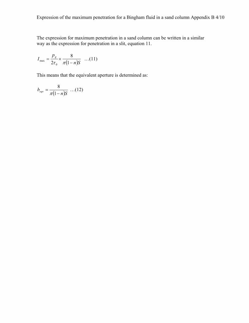
Expression of the maximum penetration for a Bingham fluid in a sand column Appendix B 4/10

The expression for maximum penetration in a sand column can be written in a similar way as the expression for penetration in a slit, equation 11.

( )Snp

I g

−×=

18

2 0max πτ

…(11)

This means that the equivalent aperture is determined as:

( )Snbeqv −

=1

8π

…(12)

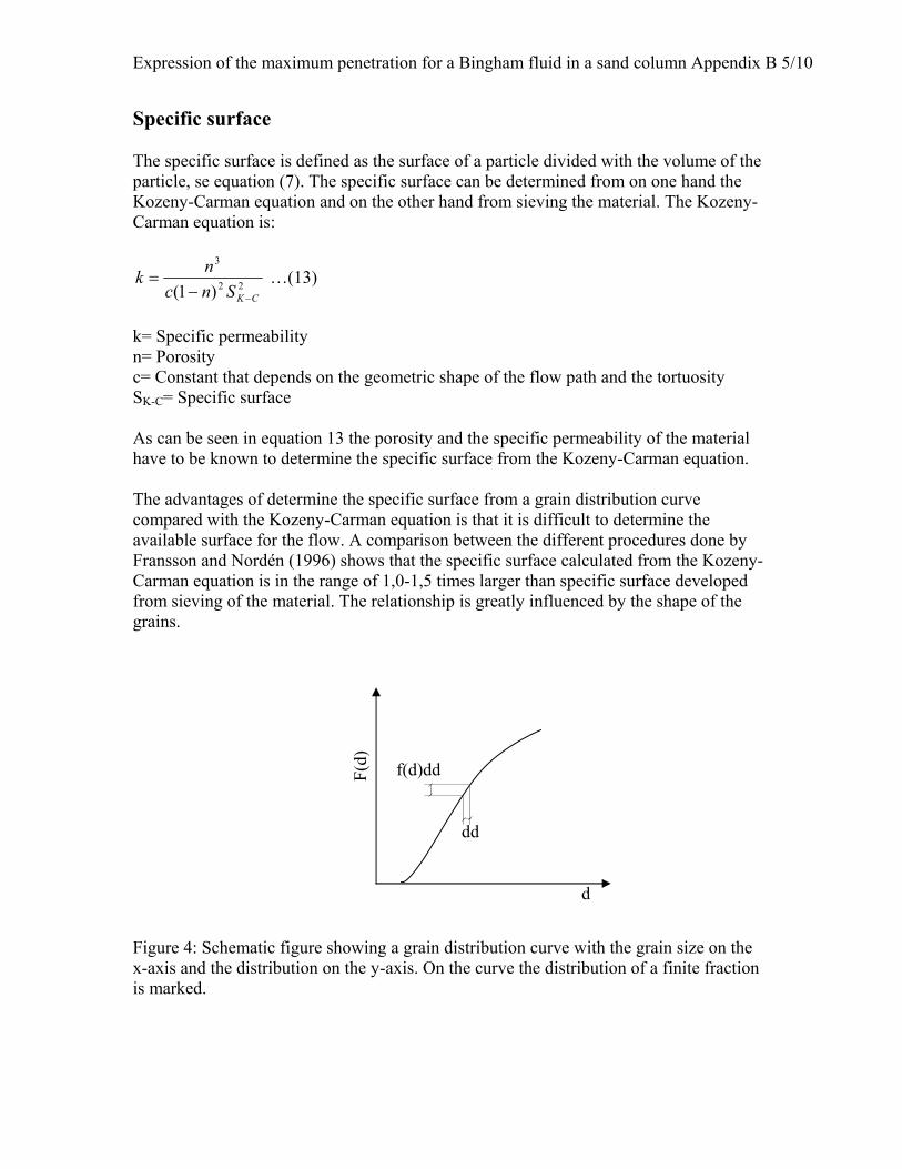
Expression of the maximum penetration for a Bingham fluid in a sand column Appendix B 5/10

Specific surface The specific surface is defined as the surface of a particle divided with the volume of the particle, se equation (7). The specific surface can be determined from on one hand the Kozeny-Carman equation and on the other hand from sieving the material. The Kozeny-Carman equation is:

22

3

)1( CKSncnk

−−= …(13)

k= Specific permeability n= Porosity c= Constant that depends on the geometric shape of the flow path and the tortuosity SK-C= Specific surface As can be seen in equation 13 the porosity and the specific permeability of the material have to be known to determine the specific surface from the Kozeny-Carman equation. The advantages of determine the specific surface from a grain distribution curve compared with the Kozeny-Carman equation is that it is difficult to determine the available surface for the flow. A comparison between the different procedures done by Fransson and Nordén (1996) shows that the specific surface calculated from the Kozeny-Carman equation is in the range of 1,0-1,5 times larger than specific surface developed from sieving of the material. The relationship is greatly influenced by the shape of the grains. Figure 4: Schematic figure showing a grain distribution curve with the grain size on the x-axis and the distribution on the y-axis. On the curve the distribution of a finite fraction is marked.

F(d)

d

f(d)dd

dd

Expression of the maximum penetration for a Bingham fluid in a sand column Appendix B 6/10

To determine an expression of the specific surface from a grain distribution curve let’s start with a schematic curve as shown in figure 4. The weight of the of the fraction, dM, that is marked in the figure can be written as:

dddfMdM )(×= …(14) dM= Mass of a fraction M= Total mass of the sample f(d)dd= Amount of the grain size dd The volume of the fraction can be determined by:

ρdMdV = …(15)

dV=Volume of the fraction ρ= Density of the material If the assumption is made that the grains are spherical, the number of grains in the fraction can be written as follows together with the connections made above:

dddfd

Md

dddfMV

dMdNg

)(6

244

)(33 πρπρ

ρ×=

×

×=

×= …(16)

dN= Number of grains in the fraction Vg= Volume of a spherical grain d= Diameter of a grain The surface of the grains within the fraction can then be expressed by using the expressions developed above.

dddfd

Mdddfdd

MddNdA )(6)(64

4 23

2

×=×××==ρ

ππρ

π …(17)

dA= Surface of the grains in the fraction From this it’s now possible to develop an expression for the surface for the whole sample by a integration over the curve.

∫∞

=0

)(6 dddfd

MAρ

…(18)

A= Surface of the grains in the whole sample But using the expression in equation 7 further developments can be done of this expression; the specific surface is defined as the surface divided by the volume.

Expression of the maximum penetration for a Bingham fluid in a sand column Appendix B 7/10

⇒=⇒= ∫∫∞∞

00

)(6)(6 dddfdV

AdddfdM

A

ρ

∫∞

=0

)(6 dddfd

S …(19)

This means that the specific surface can be defined by the integral in equation 18 that only depends on the grain distribution curve. Notice that this expression is developed for spherical grains. For a very steep grain distribution curve, well-graded material, the derivate will become 1 and the specific surface can be expressed as:

dS 6=

In many cases the grain distribution curve can be assumed as lognormal distributed (Gustafson 1983). This means that Φ=ln d and the expected value μΦ= μ and the standard deviation σΦ=σ. The standardized normal variate N [0,1] is expressed as:

σμ−Φ

=t …(20)

t= Standardized variable for N [0,1] Φ= Normal variate μ= Expected value σ= Standard deviation

Figure 5: Schematic drawing of a grain distribution curve with the 10 respectively 60 % passing grain sizes marked in the figure.

d60 d10

60%

F(d)

10%

Expression of the maximum penetration for a Bingham fluid in a sand column Appendix B 8/10

In order to describe the grain distribution curve the value of D60 and D10 (60% and 10% respectively of the material has passed the sieve) are commonly used in engineering characteration of grain curves. With the statements above and the fact that d10= F(t)= 0,1 and d60=F(t)=0,6 will give a value of the distribution function that can be received from a statistic table (Råde and Westergren, 1998). For F(t)=0,1; t=-1,28 and for F(t)=0,6; t=0,25. With this the following system of equations can be written:

μσ −=− 10ln28,1 d …(21) μσ −= 60ln25,0 d …(22)

The system of equations in equation 21 and 22 can be solved and written as:

53,1ln

ln10

60d

d

=σ …(23)

⎟⎟⎠

⎞⎜⎜⎝

⎛+=

10

6010 ln84,0ln

dd

dμ …(24)

This can thus be simplified by introduce the term U.

10

60

dd

U = …(25)

Now the expected value and the standard deviation can be described as:

53,1lnU

−=σ …(26)

Ud ln84,0ln 10 +=μ ...(27)

The harmonic mean is the inverted value of the arithmetical mean and is defined as:

⎥⎦

⎤⎢⎣

⎡+++

=

n

h

xxx

nx1...11

21

…(28)

The term xh is the harmonic mean. In a continuous function the harmonic mean can be written as:

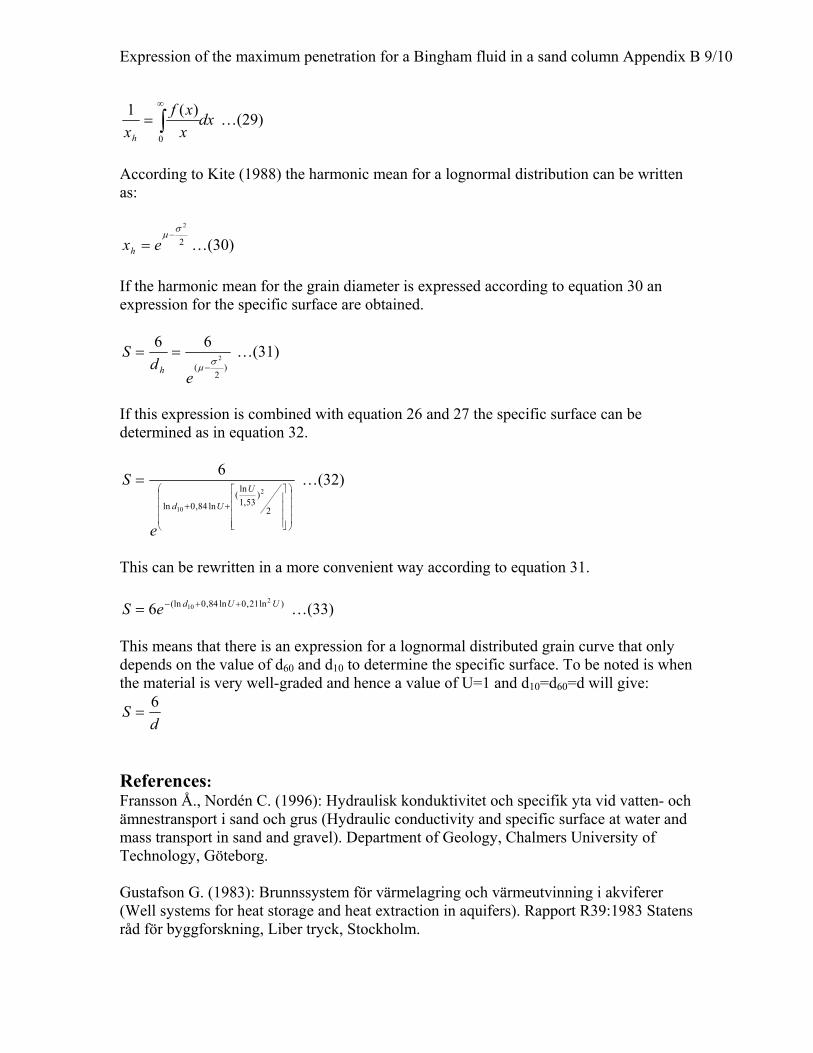
Expression of the maximum penetration for a Bingham fluid in a sand column Appendix B 9/10

dxxxf

xh∫∞

=0

)(1 …(29)

According to Kite (1988) the harmonic mean for a lognormal distribution can be written as:

2

2σμ−= exh …(30)

If the harmonic mean for the grain diameter is expressed according to equation 30 an expression for the specific surface are obtained.

)2

(2

66σ

μ−==

ed

Sh

…(31)

If this expression is combined with equation 26 and 27 the specific surface can be determined as in equation 32.

⎟⎟⎟⎟

⎠

⎞

⎜⎜⎜⎜

⎝

⎛

⎥⎥⎥⎥

⎦

⎤

⎢⎢⎢⎢

⎣

⎡

++

=

2

)53,1

ln(ln84,0ln

2

10

6U

Ud

e

S …(32)

This can be rewritten in a more convenient way according to equation 31.

)ln21,0ln84,0(ln 2106 UUdeS ++−= …(33)

This means that there is an expression for a lognormal distributed grain curve that only depends on the value of d60 and d10 to determine the specific surface. To be noted is when the material is very well-graded and hence a value of U=1 and d10=d60=d will give:

dS 6=

References: Fransson Å., Nordén C. (1996): Hydraulisk konduktivitet och specifik yta vid vatten- och ämnestransport i sand och grus (Hydraulic conductivity and specific surface at water and mass transport in sand and gravel). Department of Geology, Chalmers University of Technology, Göteborg. Gustafson G. (1983): Brunnssystem för värmelagring och värmeutvinning i akviferer (Well systems for heat storage and heat extraction in aquifers). Rapport R39:1983 Statens råd för byggforskning, Liber tryck, Stockholm.

Expression of the maximum penetration for a Bingham fluid in a sand column Appendix B 10/10

Gustafson G., Stille H (1996): Prediction of Groutability from Grout Properties and Hydrogeological Data. Tunnelling and Underground Space Technology, Vol.11, No. 3, pp.325-332. Great Britain. Kite G.W. (1988): Frequency and Risk Analyses in Hydrology. Water Resources publications, Littleton, Colorado, USA. Råde L., Westergren B. (1998):Beta- Mathematic Handbook for Science and Engineering. Studentlitteratur, Lund.

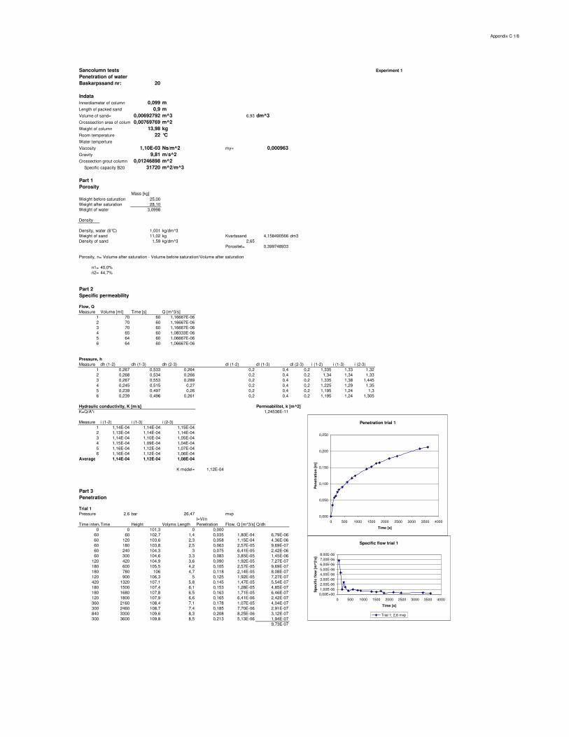
Appendix C 1/8

Sancolumn tests Experiment 1Penetration of waterBaskarpssand nr: 20

IndataInnerdiameter of column 0,099 mLength of packed sand 0,9 mVolume of sand= 0,00692792 m^3 6,93 dm^3Crosssection area of column 0,00769769 m^2Weight of column 13,98 kgRoom temperature 22 °C

Viscosity 1,10E-03 Ns/m^2 my= 0,000963Gravity 9,81 m/s^2

0,01246898 m^231720 m^2/m^3

Part 1Porosity

Mass [kg]Weight before saturation 25,00Weight after saturation 28,10Weight of water 3,0998

Density

Density, water (8°C) 1,001 kg/dm^3Weight of sand 11,02 kg Kvartssand 4,158490566 dm3Density of sand 1,59 kg/dm^3 2,65

Porositet= 0,399748933

Porosity, n= Volume after saturation - Volume before saturation/Volume after saturation

n1= 40,0%n2= 44,7%

Part 2Specific permeability

Flow, QMeasure Volume [ml] Time [s] Q [m^3/s]

1 70 60 1,16667E-062 70 60 1,16667E-063 70 60 1,16667E-064 65 60 1,08333E-065 64 60 1,06667E-066 64 60 1,06667E-06

Pressure, hMeasure dh (1-2) dh (1-3) dh (2-3) dl (1-2) dl (1-3) dl (2-3) i (1-2) i (1-3) i (2-3)

1 0,267 0,533 0,264 0,2 0,4 0,2 1,335 1,33 1,322 0,268 0,534 0,266 0,2 0,4 0,2 1,34 1,34 1,333 0,267 0,553 0,289 0,2 0,4 0,2 1,335 1,38 1,4454 0,245 0,515 0,27 0,2 0,4 0,2 1,225 1,29 1,355 0,239 0,497 0,26 0,2 0,4 0,2 1,195 1,24 1,36 0,239 0,496 0,261 0,2 0,4 0,2 1,195 1,24 1,305

Hydraulic conductivity, K [m/s] Permeabilitet, k [m^2]K=Q/A*i 1,24536E-11

Measure i (1-2) i (1-3) i (2-3)1 1,14E-04 1,14E-04 1,15E-042 1,13E-04 1,14E-04 1,14E-043 1,14E-04 1,10E-04 1,05E-044 1,15E-04 1,09E-04 1,04E-045 1,16E-04 1,12E-04 1,07E-046 1,16E-04 1,12E-04 1,06E-04

Average 1,14E-04 1,12E-04 1,08E-04

K medel= 1,12E-04

Part 3Penetration

Trial 1Pressure 2,6 bar 26,47 mvp

I=Vl/nTime intervalTime Height Volyms Length Penetration Flow, Q [m^3/s] Q/dh

0 0 101,3 0 0,00060 60 102,7 1,4 0,035 1,80E-04 6,79E-0660 120 103,6 2,3 0,058 1,15E-04 4,36E-0660 180 103,8 2,5 0,063 2,57E-05 9,69E-0760 240 104,3 3 0,075 6,41E-05 2,42E-0660 300 104,6 3,3 0,083 3,85E-05 1,45E-06

120 420 104,9 3,6 0,090 1,92E-05 7,27E-07180 600 105,5 4,2 0,105 2,57E-05 9,69E-07180 780 106 4,7 0,118 2,14E-05 8,08E-07120 900 106,3 5 0,125 1,92E-05 7,27E-07420 1320 107,1 5,8 0,145 1,47E-05 5,54E-07180 1500 107,4 6,1 0,153 1,28E-05 4,85E-07180 1680 107,8 6,5 0,163 1,71E-05 6,46E-07120 1800 107,9 6,6 0,165 6,41E-06 2,42E-07360 2160 108,4 7,1 0,178 1,07E-05 4,04E-07300 2460 108,7 7,4 0,185 7,70E-06 2,91E-07840 3300 109,6 8,3 0,208 8,25E-06 3,12E-07300 3600 109,8 8,5 0,213 5,13E-06 1,94E-07

9,73E-07

Crossection grout column

Water temperture

Specific capacity B20

Penetration trial 1

0,000

0,050

0,100

0,150

0,200

0,250

0 500 1000 1500 2000 2500 3000 3500 4000

Time [s]

Pen

etra

tion

[m]

Specific flow trial 1

0,00E+001,00E-062,00E-063,00E-064,00E-065,00E-066,00E-067,00E-068,00E-06

0 500 1000 1500 2000 2500 3000 3500 4000

Time [s]

Spe

cific

flow

[m^2

/s]

Trial 1; 2,6 mvp

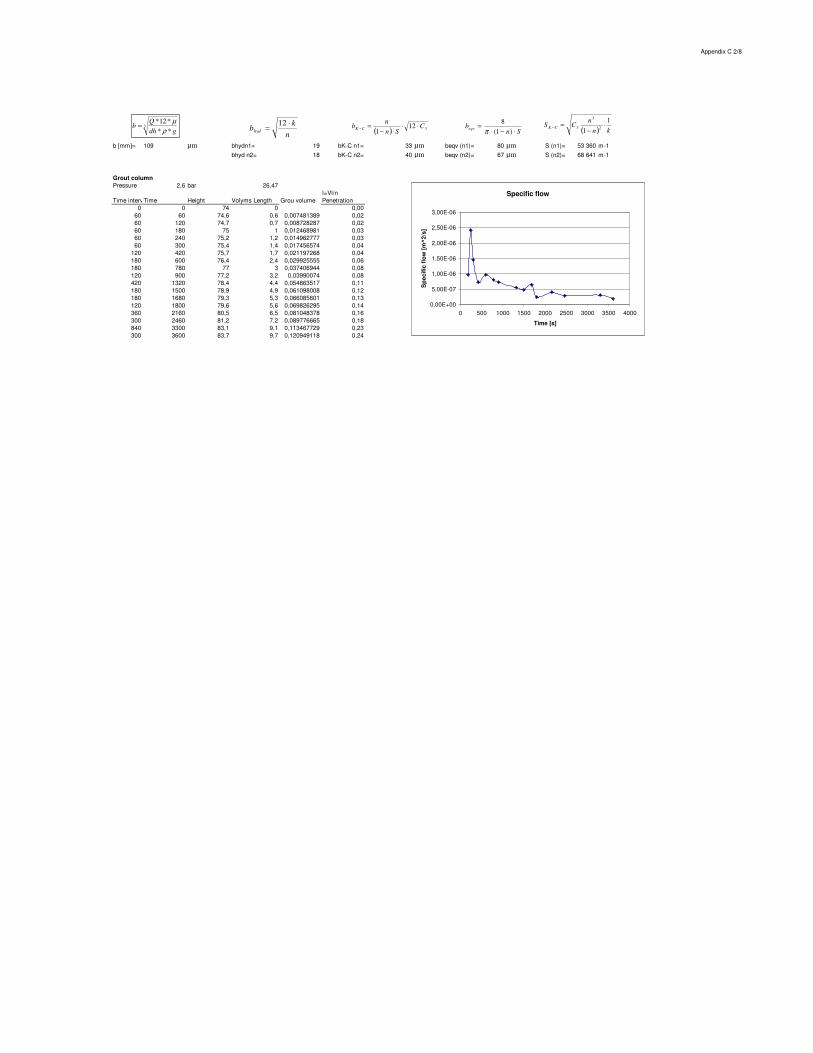
Appendix C 2/8

b [mm]= 109 µm bhydn1= 19 bK-C n1= 33 µm beqv (n1)= 80 µm S (n1)= 53 360 m-1bhyd n2= 18 bK-C n2= 40 µm beqv (n2)= 67 µm S (n2)= 68 641 m-1

Grout columnPressure 2,6 bar 26,47

I=Vl/nTime intervalTime Height Volyms Length Grou volume Penetration

0 0 74 0 0,0060 60 74,6 0,6 0,007481389 0,0260 120 74,7 0,7 0,008728287 0,0260 180 75 1 0,012468981 0,0360 240 75,2 1,2 0,014962777 0,0360 300 75,4 1,4 0,017456574 0,04

120 420 75,7 1,7 0,021197268 0,04180 600 76,4 2,4 0,029925555 0,06180 780 77 3 0,037406944 0,08120 900 77,2 3,2 0,03990074 0,08420 1320 78,4 4,4 0,054863517 0,11180 1500 78,9 4,9 0,061098008 0,12180 1680 79,3 5,3 0,066085601 0,13120 1800 79,6 5,6 0,069826295 0,14360 2160 80,5 6,5 0,081048378 0,16300 2460 81,2 7,2 0,089776665 0,18840 3300 83,1 9,1 0,113467729 0,23300 3600 83,7 9,7 0,120949118 0,24

Specific flow

0,00E+00

5,00E-07

1,00E-06

1,50E-06

2,00E-06

2,50E-06

3,00E-06

0 500 1000 1500 2000 2500 3000 3500 4000

Time [s]

Spe

cific

flow

[m^2

/s]

3***12*

gdhQ

bρ

µ= ( ) knn

CS CK

11 2

3

3 ⋅−

=−

nk

bhyd

⋅= 12( ) 3121

CSn

nb CK ⋅⋅

⋅−=− Sn

beqv ⋅−⋅=

)1(8

π

Appendix C 3/8

Sancolumn tests Experiment 2Penetration of waterBaskarpssand nr: C 40 B

IndataInnerdiameter of column 0,099 mLength of packed sand 0,9 mVolume of sand= 0,0069279 m^3 6,93 dm^3Crosssection area of column 0,0076977 m^2Weight of column 13,82 kgRoom temperature 22 °C

17,2Viscosity 1,10E-03 Ns/m^2 my= 0,001082Gravity 9,81 m/s^2

m^212820 m^2/m^3

Part 1Porosity

Mass [kg]Weight before saturation 26,62Weight after saturation 28,5

1,87Density

Density, water (8°C) 1,001 kg/dm^3Weight of sand 12,8 kg Kvartssand 4,830188679 dm3Density of sand 1,85 kg/dm^3 2,65

Porositet= 0,302793679

Porosity, n= Volume after saturation - Volume before saturation/Volume after saturation

n1= 30,3%n2= 27,0%

Part 2Specific permeability

Flow, QMeasure Volume [ml] Time [s] Q [m^3/s]

1 67,5 60 0,0000011252 68 60 1,13333E-063 68 60 1,13333E-06

Pressure, hMeasure dh (1-2) dh (1-3) dh (2-3) dl (1-2) dl (1-3) dl (2-3) i (1-2) i (1-3) i (2-3)

1 0,316 0,591 0,285 0,2 0,4 0,2 1,58 1,48 1,4252 0,313 0,597 0,285 0,2 0,4 0,2 1,565 1,49 1,4253 0,312 0,595 0,282 0,2 0,4 0,2 1,56 1,49 1,41

Hydraulic conductivity, K [m/s] Permeabilitet, k [m^2]K=Q/A*i 1,10097E-11

Measure i (1-2) i (1-3) i (2-3)1 9,25E-05 9,89E-05 1,03E-042 9,41E-05 9,86E-05 1,03E-043 9,44E-05 9,90E-05 1,04E-04

Average 9,37E-05 9,88E-05 1,03E-04K medel= 9,86E-05

Part 3Penetration

Trial 1 vct: 1,0Pressure 2,6 bar 26,47 mvp

I=Vl/nTime interval Time Height Volyms Length Penetration Flow, Q [m^3/s] Q/dh

0 0 103,9 0 0,00030 30 105,6 1,7 0,056 4,36E-04 1,65E-0560 90 106 2,1 0,069 5,13E-05 1,94E-0630 120 106,3 2,4 0,079 7,70E-05 2,91E-0660 180 106,8 2,9 0,096 6,41E-05 2,42E-0660 240 107,2 3,3 0,109 5,13E-05 1,94E-0660 300 107,4 3,5 0,116 2,57E-05 9,69E-0760 360 107,7 3,8 0,125 3,85E-05 1,45E-0660 420 107,9 4 0,132 2,57E-05 9,69E-0760 480 108,1 4,2 0,139 2,57E-05 9,69E-0760 540 108,25 4,35 0,144 1,92E-05 7,27E-0760 600 108,4 4,5 0,149 1,92E-05 7,27E-07

240 840 108,9 5 0,165 1,60E-05 6,06E-0760 900 109 5,1 0,168 1,28E-05 4,85E-07

120 1020 109,25 5,35 0,177 1,60E-05 6,06E-07180 1200 109,5 5,6 0,185 1,07E-05 4,04E-07180 1380 109,8 5,9 0,195 1,28E-05 4,85E-07120 1500 110 6,1 0,201 1,28E-05 4,85E-07120 1620 110,1 6,2 0,205 6,41E-06 2,42E-07180 1800 110,2 6,3 0,208 4,28E-06 1,62E-07420 2220 110,7 6,8 0,225 9,16E-06 3,46E-07180 2400 110,8 6,9 0,228 4,28E-06 1,62E-07300 2700 111,05 7,15 0,236 6,41E-06 2,42E-07300 3000 111,25 7,35 0,243 5,13E-06 1,94E-07300 3300 111,4 7,5 0,248 3,85E-06 1,45E-07300 3600 111,6 7,7 0,254 5,13E-06 1,94E-07

8,24E-07

Crossection grout column

Water temperture

Specific capacity C40B

Penetration trial 2

0,000

0,050

0,100

0,150

0,200

0,250

0,300

0 1000 2000 3000 4000

Time [s]

Pen

etra

tion

[m]

Specific flow trial 2

0,00E+00

2,00E-06

4,00E-06

6,00E-06

8,00E-06

1,00E-05

1,20E-05

1,40E-05

1,60E-05

1,80E-05

0 500 1000 1500 2000 2500 3000 3500 4000

Time [s]

Spe

cific

flow

[m^2

/s]

Trial 1; 2,6 mvp

Appendix C 4/8

b cubic= 109 µm bhyd n1= 21 bK-C n1= 52 µm beqv (n1)= 113 µm S (n1)= 32 210 m-1bhyd n2= 22 bK-C n2= 45 µm beqv (n2)= 135 µm S (n2)= 25 889 m-1

Grout columnPressure 2,6 bar 26,47

I=Vl/nTime interval Time Height Volyms Length Grou volume Penetration

0 0 74 0 0,0060 60 -74 0 -244,39

Specific flow

0,00E+00

5,00E-07

1,00E-06

1,50E-06

2,00E-06

2,50E-06

3,00E-06

3,50E-06

0 500 1000 1500 2000 2500 3000 3500 4000

Time [s]

Spe

cifi

c fl

ow [

m^2

/s]

Trial 1; 2,6 mvp without first 2 values

3***12*

gdhQ

bρ

µ=( ) kn

nCS CK

11 2

3

3 ⋅−

=−n

kbhyd

⋅= 12( ) 3121

CSn

nb CK ⋅⋅

⋅−=−

Snbeqv ⋅−⋅

=)1(

8π

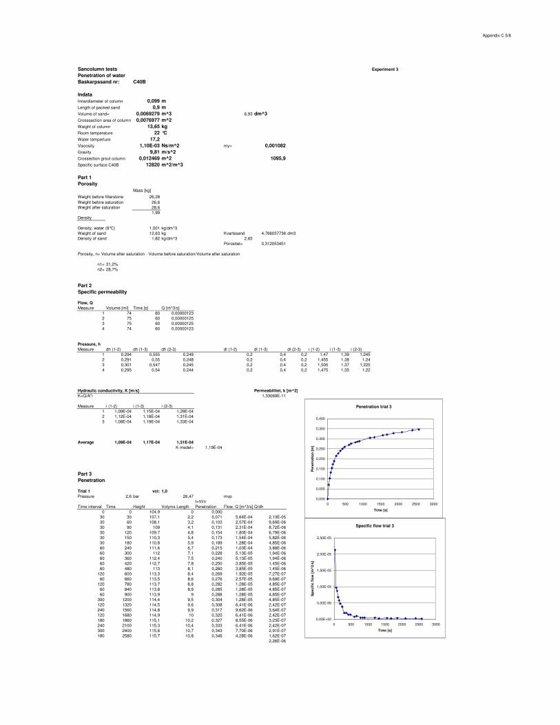
Appendix C 5/8

Sancolumn tests Experiment 3Penetration of waterBaskarpssand nr: C40B

IndataInnerdiameter of column 0,099 mLength of packed sand 0,9 mVolume of sand= 0,0069279 m^3 6,93 dm^3Crosssection area of column 0,0076977 m^2Weight of column 13,65 kgRoom temperature 22 °C

17,2Viscosity 1,10E-03 Ns/m^2 my= 0,001082Gravity 9,81 m/s^2

0,012469 m^2 1095,912820 m^2/m^3

Part 1Porosity

Mass [kg]Weight before filterstone 26,28Weight before saturation 26,6Weight after saturation 28,6

1,99Density

Density, water (8°C) 1,001 kg/dm^3Weight of sand 12,63 kg Kvartssand 4,766037736 dm3Density of sand 1,82 kg/dm^3 2,65

Porositet= 0,312053451

Porosity, n= Volume after saturation - Volume before saturation/Volume after saturation

n1= 31,2%n2= 28,7%

Part 2Specific permeability

Flow, QMeasure Volume [ml] Time [s] Q [m^3/s]

1 74 60 0,000001232 75 60 0,000001253 75 60 0,000001254 74 60 0,00000123

Pressure, hMeasure dh (1-2) dh (1-3) dh (2-3) dl (1-2) dl (1-3) dl (2-3) i (1-2) i (1-3) i (2-3)

1 0,294 0,555 0,249 0,2 0,4 0,2 1,47 1,39 1,2452 0,291 0,55 0,248 0,2 0,4 0,2 1,455 1,38 1,243 0,301 0,547 0,245 0,2 0,4 0,2 1,505 1,37 1,2254 0,295 0,54 0,244 0,2 0,4 0,2 1,475 1,35 1,22

Hydraulic conductivity, K [m/s] Permeabilitet, k [m^2]K=Q/A*i 1,33069E-11

Measure i (1-2) i (1-3) i (2-3)1 1,09E-04 1,15E-04 1,29E-042 1,12E-04 1,18E-04 1,31E-043 1,08E-04 1,19E-04 1,33E-04

Average 1,09E-04 1,17E-04 1,31E-04K medel= 1,19E-04

Part 3Penetration

Trial 1 vct: 1,0Pressure 2,6 bar 26,47 mvp

I=Vl/nTime interval Time Height Volyms Length Penetration Flow, Q [m^3/s] Q/dh

0 0 104,9 0 0,00030 30 107,1 2,2 0,071 5,64E-04 2,13E-0530 60 108,1 3,2 0,103 2,57E-04 9,69E-0630 90 109 4,1 0,131 2,31E-04 8,72E-0630 120 109,7 4,8 0,154 1,80E-04 6,79E-0630 150 110,3 5,4 0,173 1,54E-04 5,82E-0630 180 110,8 5,9 0,189 1,28E-04 4,85E-0660 240 111,6 6,7 0,215 1,03E-04 3,88E-0660 300 112 7,1 0,228 5,13E-05 1,94E-0660 360 112,4 7,5 0,240 5,13E-05 1,94E-0660 420 112,7 7,8 0,250 3,85E-05 1,45E-0660 480 113 8,1 0,260 3,85E-05 1,45E-06

120 600 113,3 8,4 0,269 1,92E-05 7,27E-0760 660 113,5 8,6 0,276 2,57E-05 9,69E-07

120 780 113,7 8,8 0,282 1,28E-05 4,85E-0760 840 113,8 8,9 0,285 1,28E-05 4,85E-0760 900 113,9 9 0,288 1,28E-05 4,85E-07

300 1200 114,4 9,5 0,304 1,28E-05 4,85E-07120 1320 114,5 9,6 0,308 6,41E-06 2,42E-07240 1560 114,8 9,9 0,317 9,62E-06 3,64E-07120 1680 114,9 10 0,320 6,41E-06 2,42E-07180 1860 115,1 10,2 0,327 8,55E-06 3,23E-07240 2100 115,3 10,4 0,333 6,41E-06 2,42E-07300 2400 115,6 10,7 0,343 7,70E-06 2,91E-07180 2580 115,7 10,8 0,346 4,28E-06 1,62E-07

2,26E-06

Crossection grout column

Water temperture

Specific surface C40B

Penetration trial 3

0,000

0,050

0,100

0,150

0,200

0,250

0,300

0,350

0,400

0 500 1000 1500 2000 2500 3000

Time [s]

Pen

etra

tion

[m]

Specific flow trial 3

0,00E+00

5,00E-06

1,00E-05

1,50E-05

2,00E-05

2,50E-05

0 500 1000 1500 2000 2500 3000

Time [s]

Spe

cific

flow

[m^2

/s]

Appendix C 6/8

b cubic = 153 µm bhyd n1= 23 bK-C n1= 55 µm beqv (n1)= 1,19E-04 µm S (n1)= 31 065 m-1bhyd n2= 24 bK-C n2= 49 µm beqv (n2)= 1,35E-04 µm S (n2)= 26 480 m-1

Grout columnPressure 2,6 bar 26,47

I=Vl/nTime interval Time Height Volyms Length Grou volume Penetration

0 0 65,5 0 0,0030 30 72,9 7,4 0,092270461 0,2430 60 73,1 7,6 0,094764257 0,2430 90 75 9,5 0,118455322 0,3030 120 75,3 9,8 0,122196016 0,3130 150 75,6 10,1 0,125936711 0,3230 180 75,7 10,2 0,127183609 0,3360 240 76,1 10,6 0,132171201 0,3460 300 76,5 11 0,137158794 0,3560 360 76,8 11,3 0,140899488 0,3660 420 77,2 11,7 0,145887081 0,3760 480 77,3 11,8 0,147133979 0,38

120 600 77,7 12,2 0,152121571 0,3960 660 77,8 12,3 0,153368469 0,39

120 780 78,1 12,6 0,157109164 0,4060 840 78,2 12,7 0,158356062 0,4160 900 78,4 12,9 0,160849858 0,41

300 1200 79,3 13,8 0,172071941 0,44120 1320 79,7 14,2 0,177059534 0,46240 1560 80,2 14,7 0,183294024 0,47120 1680 80,5 15 0,187034719 0,48180 1860 80,8 15,3 0,190775413 0,49240 2100 81,3 15,8 0,197009904 0,51300 2400 82 16,5 0,20573819 0,53180 2580 82,4 16,9 0,210725783 0,54

Specific flow

0,00E+00

1,00E-06

2,00E-06

3,00E-06

4,00E-06

5,00E-06

6,00E-06

7,00E-06

8,00E-06

9,00E-06

1,00E-05

0 500 1000 1500 2000 2500 3000

Time [s]

Spe

cific

flow

[m^2

/s]

Trial 1; 2,6 mvp without first 2 values

3***12*

gdhQ

bρ

µ=( ) kn

nCS CK

11 2

3

3 ⋅−

=−nk

bhyd

⋅= 12

( ) 3121

CSn

nb CK ⋅⋅

⋅−=− Sn

beqv ⋅−⋅=

)1(8

π

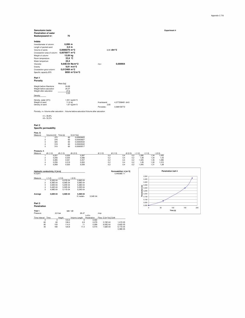
Appendix C 7/8

Sancolumn tests Experiment 4Penetration of waterBaskarpssand nr: 70

IndataInnerdiameter of column 0,099 mLength of packed sand 0,9 mVolume of sand= 0,0069279 m^3 6,93 dm^3Crosssection area of column 0,0076977 m^2Weight of column 13,09 kgRoom temperature 22,6 °C

22,4Viscosity 9,64E-04 Ns/m^2 my= 0,000954Gravity 9,81 m/s^2

0,012469 m^29050 m^2/m^3

Part 1Porosity

Mass [kg]Weight before filterstone 24,69Weight before saturation 25,37Weight after saturation 27,6

2,23Density

Density, water (8°C) 1,001 kg/dm^3Weight of sand 11,6 kg Kvartssand 4,377358491 dm3Density of sand 1,67 kg/dm^3 2,65

Porositet= 0,368156772

Porosity, n= Volume after saturation - Volume before saturation/Volume after saturation

n1= 36,8%n2= 32,2%

Part 2Specific permeability

Flow, QMeasure Volume [ml] Time [s] Q [m^3/s]

1 375 60 0,000006252 376 60 0,000006273 325 60 0,000005424 319 60 0,000005325 310 60 0,00000517

Pressure, hMeasure dh (1-2) dh (1-3) dh (2-3) dl (1-2) dl (1-3) dl (2-3) i (1-2) i (1-3) i (2-3)

1 0,257 0,535 0,287 0,2 0,4 0,2 1,285 1,34 1,4352 0,256 0,535 0,286 0,2 0,4 0,2 1,28 1,34 1,433 0,285 0,541 0,257 0,2 0,4 0,2 1,425 1,35 1,2854 0,256 0,519 0,263 0,2 0,4 0,2 1,28 1,30 1,3155 0,269 0,525 0,256 0,2 0,4 0,2 1,345 1,31 1,28

Hydraulic conductivity, K [m/s] Permeabilitet, k [m^2]K=Q/A*i 5,44008E-11

Measure i (1-2) i (1-3) i (2-3)1 6,32E-04 6,07E-04 5,66E-042 6,36E-04 6,09E-04 5,69E-043 4,94E-04 5,20E-04 5,48E-044 5,40E-04 5,32E-04 5,25E-045 4,99E-04 5,11E-04 5,24E-04

Average 5,60E-04 5,56E-04 5,46E-04K medel= 5,54E-04

Part 3Penetration

Trial 1 vct: 1,0Pressure 2,6 bar 26,47 mvp

I=Vl/nTime interval Time Height Volyms Length Penetration Flow, Q [m^3/s] Q/dh

0 0 103,5 0 0,00060 60 106,4 2,9 0,079 3,72E-04 1,41E-0590 150 114,5 11 0,299 6,93E-04 2,62E-0530 180 120,8 17,3 0,470 1,62E-03 6,11E-05

3,38E-05

Crossection grout column

Water temperture

Specific capacity B70

Penetration trail 4

0,000

0,050

0,100

0,150

0,200

0,250

0,300

0,350

0,400

0,450

0,500

0 50 100 150 200

Time [s]

Pen

etra

tion

[m]

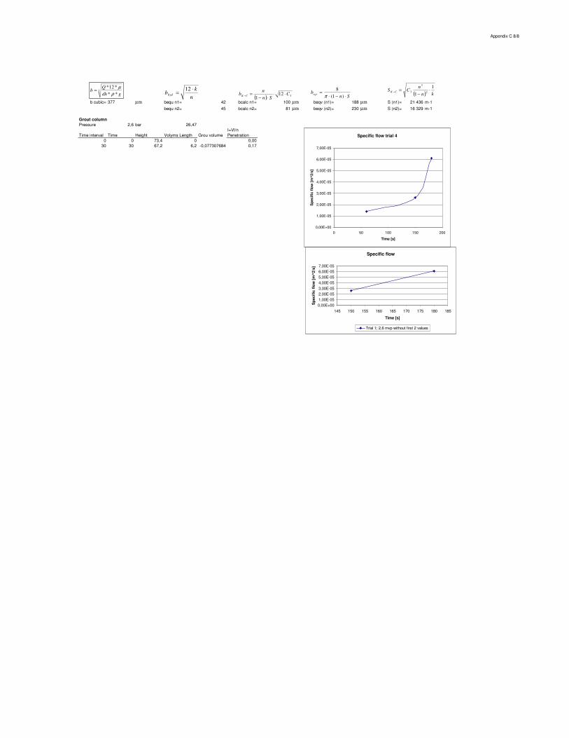
Appendix C 8/8

b cubic= 377 µm bequ n1= 42 bcalc n1= 100 µm beqv (n1)= 188 µm S (n1)= 21 436 m-1bequ n2= 45 bcalc n2= 81 µm beqv (n2)= 230 µm S (n2)= 16 329 m-1

Grout columnPressure 2,6 bar 26,47

I=Vl/nTime interval Time Height Volyms Length Grou volume Penetration

0 0 73,4 0 0,0030 30 67,2 6,2 -0,077307684 0,17

Specific flow

0,00E+001,00E-052,00E-053,00E-054,00E-055,00E-056,00E-057,00E-05

145 150 155 160 165 170 175 180 185

Time [s]S

peci

fic

flow

[m

^2/s

]

Trial 1; 2,6 mvp without first 2 values

3***12*

gdhQ

bρ

µ=

Specific flow trial 4

0,00E+00

1,00E-05

2,00E-05

3,00E-05

4,00E-05

5,00E-05

6,00E-05

7,00E-05

0 50 100 150 200

Time [s]

Spe

cific

flow

[m^2

/s]

( ) knn

CS CK

11 2

3

3 ⋅−

=−

nk

bhyd

⋅= 12

( ) 3121

CSn

nb CK ⋅⋅

⋅−=− Sn

beqv ⋅−⋅=

)1(8

π

Development of expression for growth of a filter cake Appendix D 1/3

Expression for the growth of a filter cake In Figure D.1., the process of a growing filter cake is shown. The filter cake has a thickness of θ and is growing with dθ. Into the filter cake is a suspension flowing with the concentration, C of grains in the water. The total flow is Q and the flow area is A. The growth of the filter cake can be expressed as:

ACQ

dtd ⋅

=θ D.1.

The flow according to Darcy’s law can be expressed as:

AKgpAK

dldhQ

w

⋅⋅⋅⋅

Δ=⋅⋅−=

θρ. D.2.

Figure D.1. Filter cake with thickness θ and increased thickness of dθ as a suspension flow through a pipe with area of A. The driving force is expressed as Δp and the hydraulic conductivity is K. Combining these expressions results in that the growth of the filter cake is:

ACAK

gp

dtd

w

⋅⋅⋅⋅⋅

Δ=

θρθ . D.3.

θ

dθ

Filter cake

Water

Suspension

Development of expression for growth of a filter cake Appendix D 2/3

By simplifying this expression and further refine it by considering a part as constant, the expression becomes:

dtconstdtg

CKpdw

⋅=⋅⋅⋅⋅Δ

=⋅ρ

θθ D.4.

Integrating this according to Equation D.5. yields an expression according to Equation D.6.

∫ ∫ ⋅=⋅ dtconstdθθ D.5.

tconst ⋅=2

2θ D.6.

This means that the thickness of the filter cake can be expressed as :

tconst ⋅⋅= 2θ D.7. By combining Equation D.2. with the expression obtained in Equation D.7., the flow can be expressed as:

AKt

gCKpg

pQ

ww

⋅⋅⋅

⋅⋅⋅Δ

⋅⋅⋅

Δ=

ρρ 2

D.8.

Simplifying this expression yields:

tCgKpAQ

w

12

⋅⋅⋅⋅

⋅Δ⋅=

ρ D.9.

The volume of material in the filter cake can be expressed by integrating over time and the result becomes:

tCg

KpAdttCg

KpAdtQVww

t

22

120

⋅⋅⋅⋅

⋅Δ⋅=⋅⋅

⋅⋅⋅⋅Δ

⋅=⋅= ∫ ρρ. D.10.

Development of expression for growth of a filter cake Appendix D 3/3

The expression developed in Equation D.10. implies that the volume of the filter cake is proportional to the square root of time. This can be schematically described according to Figure D.2. The volume or penetration of the suspension is initially increasing fast but after some time the curve is flatten-out and becomes proportional to the square of the time, indicating that the process of forming filter cake have been initialised. Figure D.2. The volume or penetration of suspension versus the square of time. As the penetration curve is proportional (linear) with the square of time, the forming of a filter cake can be expected.

V

t2