Grouped Patterns of Heterogeneity in Panel Data

The MIT Faculty has made this article openly available. Please share how this access benefits you. Your story matters.

Citation Bonhomme, Stéphane, and Manresa, Elena. “Grouped Patterns ofHeterogeneity in Panel Data.” Econometrica 83, 3 (May 2015): 1147–1184 © 2015 The Econometric Society

As Published http://dx.doi.org/10.3982/ecta11319

Publisher The Econometric Society

Version Author's final manuscript

Citable link http://hdl.handle.net/1721.1/111106

Terms of Use Creative Commons Attribution-Noncommercial-Share Alike

Detailed Terms http://creativecommons.org/licenses/by-nc-sa/4.0/

Grouped Patterns of Heterogeneity in Panel Data∗

Stephane Bonhomme

University of Chicago

Elena Manresa

MIT Sloan

Final version: December 2014

Abstract

This paper introduces time-varying grouped patterns of heterogeneity in linear panel data mod-

els. A distinctive feature of our approach is that group membership is left unrestricted. We estimate

the parameters of the model using a “grouped fixed-effects” estimator that minimizes a least-squares

criterion with respect to all possible groupings of the cross-sectional units. Recent advances in the

clustering literature allow for fast and efficient computation. We provide conditions under which

our estimator is consistent as both dimensions of the panel tend to infinity, and we develop inference

methods. Finally, we allow for grouped patterns of unobserved heterogeneity in the study of the

link between income and democracy across countries.

JEL codes: C23.

Keywords: Discrete heterogeneity, panel data, fixed effects, clustering, democracy.

∗We thank the co-editor Elie Tamer and two anonymous referees for their help in improving the paper. We also thank

Daron Acemoglu, Daniel Aloise, Dante Amengual, Manuel Arellano, Jushan Bai, Alan Bester, Fabio Canova, Victor

Chernozhukov, Denis Chetverikov, David Dorn, Kirill Evdokimov, Ivan Fernandez-Val, Lars Hansen, Jim Heckman,

Han Hong, Bo Honore, Andrea Ichino, Jacques Mairesse, Monica Martınez-Bravo, Serena Ng, Taisuke Otsu, Eleonora

Patacchini, Peter Phillips, Jean-Marc Robin, Enrique Sentana, Martin Weidner, and seminar participants at various

venues for useful comments. Support from the European Research Council/ ERC grant agreement n0263107 and from

the Ministerio de Economıa y Competitividad Grant ECO2011 − 26342 is gratefully acknowledged. All errors are our

own.

1 Introduction

There is ample evidence that workers, firms or countries differ in many dimensions that are unob-

servable to the econometrician. In practice, applied researchers face a trade-off between using flexible

approaches to model unobserved heterogeneity, and building parsimonious specifications that are well

adapted to the data at hand. The goal of this paper is to propose a flexible yet parsimonious approach

to allow for unobserved heterogeneity in a panel data context.

A common approach is to model heterogeneity as unit-specific, time-invariant fixed-effects. Fixed-

effects approaches are attractive as they allow for unrestricted correlation between unobserved effects

and covariates. However, in models with as many parameters as individual units, estimates of common

parameters are subject to an “incidental parameter” bias that may be substantial in short panels

(Nickel, 1981), and the fixed-effects themselves are often poorly estimated. In addition, standard fixed-

effects approaches are arguably restrictive as they assume that unobserved heterogeneity is constant

over time.

This paper proposes a framework that allows for clustered time patterns of unobserved heterogene-

ity that are common within groups of individuals. The group-specific time patterns and individual

group membership are left unrestricted, and are estimated from the data. In particular, as in fixed-

effects, our time-varying specification allows for general forms of covariates endogeneity. The main

assumption is that the number of distinct individual time patterns of unobserved heterogeneity is

relatively small.

A simple linear model with grouped patterns of heterogeneity takes the following form:

yit = x′itθ + αgit + vit, i = 1, ..., N, t = 1, ..., T, (1)

where the covariates xit are contemporaneously uncorrelated with vit, but may be arbitrarily correlated

with the group-specific unobservables αgit. The group membership variables gi ∈ 1, ..., G and the

group-specific time effects αgt, for g ∈ 1, .., G, are unrestricted. Units in the same group share the

same time profile αgt (for example, all i such that gi = 1 share the profile α1t). The number of groups

G is to be set or estimated by the researcher. Beyond model (1) we study in detail two extensions:

a model with additive time-invariant fixed-effects ηi in addition to the time-varying grouped effects

αgit, and a model with group-specific coefficients θgi .

Potential applications of model (1) and its extensions include social interaction models for panel

data where group-level interactions are subsumed in αgit (Blume et al., 2010), or tests of full risk-

sharing in village economies (Townsend, 1994). Unlike most applications of social interactions and

risk sharing, our approach allows to estimate the reference groups, under the assumption that group

membership remains constant over time. In a different perspective, grouped patterns of heterogeneity

can be useful to model interdependence across individual units over time. Compared with existing

spatial dependence models for panel data (e.g., Sarafidis and Wansbeek, 2012), model (1) allows the

1

researcher to estimate the spatial weights matrix.

Our estimator, which we will refer to as “grouped fixed-effects” (GFE), is based on an optimal

grouping of theN cross-sectional units, according to a least-squares criterion. Units whose time profiles

of outcomes– net of the effect of covariates– are most similar are grouped together in estimation. In

the absence of covariates in model (1), the estimation problem coincides with the standard minimum

sum-of-squares partitioning problem, and a simple computational method is given by the “kmeans”

algorithm (Forgy, 1965, Steinley, 2006). We take advantage of recent advances in the clustering

literature to build fast and reliable computational routines.1

We derive the statistical properties of the grouped fixed-effects estimator in an asymptotic where

N and T tend to infinity simultaneously. In our framework, N can grow substantially faster than

T , in contrast with models with unit-specific fixed-effects. While fixed-effects estimators generally

suffer from a O(1/T) bias as N/T tends to a constant (Arellano and Hahn, 2007), we show that

the GFE estimator is consistent and asymptotically normal as N/T ν tends to zero for some ν > 0,

provided groups are well separated and errors vit satisfy suitable tail and dependence conditions. This

property, which has also been noted in models with time-invariant discrete heterogeneity (Hahn and

Moon, 2010), is a consequence of group classification improving very fast as the number of time periods

increases. In particular, our results provide a formal justification for clustering methods.2

As the two dimensions of the panel diverge, the GFE estimator is asymptotically equivalent to

the infeasible least squares estimator with known population groups. As a consequence, in a large-T

perspective standard errors are unaffected by the fact that group membership has been estimated. In

short panels, however, group misclassification may contribute to the finite-sample dispersion of the

estimator. For this reason, we also study the properties of the GFE estimator for fixed T as N tends

to infinity. In a Monte Carlo exercise calibrated to the empirical application, we provide evidence

that using the GFE estimator in combination with an estimate of its fixed-T variance yields reliable

inference for the population parameters.

We use our approach to study the effect of income on democracy in a panel of countries that spans

the last part of the twentieth century. In an influential paper, Acemoglu et al. (2008) find that the

positive association between income and democracy disappears when controlling for additive country-

and time-effects. They interpret the country fixed-effects as reflecting long-run, historical factors that

have shaped the political and economic development of countries.

In the context of this application, the grouped fixed-effects model allows for time-varying unob-

servables in a period that is characterized by a large number of transitions to democracy, and it is well

suited to deal with the short length of the panel (T = 7). Grouped patterns are also consistent with

1Stata codes, which make use of a Fortran executable program, are available as supplementary material.2Related results in statistics include Pollard (1981, 1982) on minimum sum-of-squares partitioning, and Bryant and

Williamson (1978) in a class of likelihood models. To our knowledge, ours is the first paper to establish conditions under

which the clustering estimator in kmeans becomes consistent as N and T tend to infinity.

2

the empirical observation that regime types and transitions tend to cluster in time and space (e.g.,

Gleditsch and Ward, 2006, Ahlquist and Wibbels, 2012). An early conceptual framework is laid out

in Huntington (1991)’s work on the “third wave of democracy”, which argues that international and

regional factors– such as the influence of the Catholic Church or the European Union– may have in-

duced grouped patterns of democratization. We find robust evidence of heterogeneous, group-specific

paths of democratization in the data.

Related literature and outline. Our modelling of grouped heterogeneity is related to, but different

from, finite mixture models. These models rely on assumptions that restrict the relationship between

unobserved heterogeneity and covariates.3 In contrast, and in close analogy with fixed-effects, our

approach leaves that relationship unspecified. In fact, the group membership variables gi may be

viewed as indexing the N time-varying paths of unit-specific unobserved heterogeneity. The key

assumption is that at most G of these paths are distinct from each other. This imposes a restriction

on the support of unobserved heterogeneity, while leaving other features of the relationship with

observables unrestricted.4

The grouped fixed-effects model is also related to factor-analytic, “interactive fixed-effects” models

(Bai, 2009). Indeed, model (1) has a factor-analytic structure, as: αgit =∑G

g=1 1gi = gαgt. We take

advantage of this mathematical connection to establish consistency of the GFE estimator, and to study

a class of information criteria to select the number of groups. Our theoretical and numerical results

suggest that, in relatively short panels and when the data have a grouped structure, the parsimony of

the GFE estimator may provide a useful alternative to interactive fixed-effects.

Finally, this paper is not the first one to rely on grouped structures for modelling unobserved

heterogeneity in panels. Bester and Hansen (2013) show that grouping individual fixed-effects can

result in gains in precision, in a setup where the grouping of the data is known. Lin and Ng (2012)

consider a random coefficients model and use the time-series regression estimates to classify individual

units into several groups. None of these two papers allows for time-varying unobserved heterogeneity.5

The outline of the paper is as follows. We introduce the grouped fixed-effects estimator in Section 2.

We derive its asymptotic properties in Section 3. We use the GFE approach to study the relationship

between income and democracy in Section 4, and conclude in Section 5. Additional material may be

found in a supplementary appendix.

3See the monographs by McLachlan and Peel (2000) and Fruhwirth-Schnatter (2006) for recent advances in this area.4In this sense, our approach is reminiscent of sparsity assumptions in the literature on high-dimensional modelling

(e.g., Tibshirani, 1996).5Group models and clustering approaches have also been used to search for “convergence clubs” in the empirical

growth literature; see for example Canova (2004), and Phillips and Sul (2007). See also Sun (2005). Similar techniques

have been proposed in the statistical analysis of network data (e.g., Bickel and Chen, 2009, Choi et al., 2012).

3

2 The grouped fixed-effects estimator

In the first part of this section we introduce the grouped fixed-effects (GFE) estimator in several

models. In the second part we provide computational methods.

2.1 Models and estimators

Model (1) contains three types of parameters: the parameter vector θ ∈ Θ, which is common across

individual units; the group-specific time effects αgt ∈ A, for all g ∈ 1, ..., G and all t ∈ 1, ..., T;and the group membership variables gi, for all i ∈ 1, ..., N, which map individual units into groups.

The parameter spaces Θ and A are subsets of RK and R, respectively. We denote as α the set of all

αgt’s, and as γ the set of all gi’s. Thus, γ ∈ ΓG denotes a particular grouping (i.e., partition) of the

N units, where ΓG is the set of all groupings of 1, ..., N into at most G groups.

The covariates vector xit may include strictly exogenous regressors and lagged outcomes. The

model also allows for time-invariant regressors under certain support conditions. Moreover, xit and

αgit are allowed to be arbitrarily correlated. We will state precise conditions in the next section.

The grouped fixed-effects estimator in model (1) is defined as the solution of the following mini-

mization problem:

(θ, α, γ

)= argmin

(θ,α,γ)∈Θ×AGT×ΓG

N∑

i=1

T∑

t=1

(yit − x′itθ − αgit

)2, (2)

where the minimum is taken over all possible groupings γ = g1, ..., gN of the N units into G groups,

common parameters θ, and group-specific time effects α.

For given values of θ and α, the optimal group assignment for each individual unit is:

gi (θ, α) = argming∈1,...,G

T∑

t=1

(yit − x′itθ − αgt

)2, (3)

where we take the minimum g in case of a non-unique solution. The GFE estimator of (θ, α) in (2)

can then be written as:

(θ, α

)= argmin

(θ,α)∈Θ×AGT

N∑

i=1

T∑

t=1

(yit − x′itθ − αgi(θ,α)t

)2, (4)

where gi (θ, α) is given by (3). The GFE estimate of gi is then simply gi

(θ, α

).

Unlike standard finite mixture modelling, which specifies the group probabilities as parametric

or semiparametric functions of observed covariates (e.g., McLachlan and Peel, 2000), grouped fixed-

effects leaves group membership unrestricted. In the supplementary appendix we show that the GFE

estimator maximizes the pseudo-likelihood of a mixture-of-normals model, where the mixing probabil-

ities are unrestricted and individual-specific. In this perspective, the grouped fixed-effects approach

may be seen as a point of contact between finite mixtures and fixed-effects.

4

Extension 1: unit-specific heterogeneity. The GFE framework can be combined with additive

time-invariant fixed-effects:

yit = x′itθ + αgit + ηi + vit, (5)

where ηi are N unrestricted parameters. Letting wi =1T

∑Tt=1wit, the following equation in deviations

to the mean:

yit − yi = (xit − xi)′ θ + αgit − αgi + vit − vi, (6)

has the same structure as model (1), and can be estimated using grouped fixed-effects.

Extension 2: heterogeneous coefficients. Another extension is to allow for group-specific effects

of covariates:

yit = x′itθgi + αgit + vit, (7)

and define the following GFE estimator:

(θ, α, γ

)= argmin

(θ,α,γ)∈ΘG×AGT×ΓG

N∑

i=1

T∑

t=1

(yit − x′itθgi − αgit

)2, (8)

where here θ contains all θg’s.

Other extensions of the baseline model are possible. For example, one could allow for unit-specific

heterogeneity and heterogeneous coefficients at the same time. In addition, in the supplementary

appendix we show how to incorporate prior information on the groups or the group-specific time

effects when such information is available.

Nonlinear models. Grouped patterns of heterogeneity may be introduced in nonlinear models as

well. A general M-estimator formulation based on a data-dependent function mit(·) is as follows:

(θ, α, γ

)= argmin

(θ,α,γ)∈ΘG×AGT×ΓG

N∑

i=1

T∑

t=1

mit (θ, αt, gi) . (9)

This framework covers likelihood models as special cases.6 In particular, it encompasses static and

dynamic discrete choice models. However, studying the statistical properties of GFE in nonlinear

models exceeds the scope of this paper.

2.2 Computation

One can see, from (4), that the grouped fixed-effects estimator minimizes a piecewise-quadratic func-

tion, where the partition of the parameter space is defined by the different values of gi (θ, α), for

6A GFE estimator in a likelihood setup is obtained by taking mit (θ, αt, gi) = − ln f (yit|xit; θ, αt, gi), where f(·)denotes a parametric density function.

5

i = 1, ..., N . However, the number of partitions of N units into G groups increases steeply with N ,

making exhaustive search virtually impossible.

The following algorithm uses a simple iterative strategy to minimize (4).

Algorithm 1 (iterative)

1. Let(θ(0), α(0)

)∈ Θ×AGT be some starting value. Set s = 0.

2. Compute for all i ∈ 1, ..., N:

g(s+1)i = argmin

g∈1,...,G

T∑

t=1

(yit − x′itθ

(s) − α(s)gt

)2. (10)

3. Compute:(θ(s+1), α(s+1)

)= argmin

(θ,α)∈Θ×AGT

N∑

i=1

N∑

t=1

(yit − x′itθ − α

g(s+1)i t

)2. (11)

4. Set s = s+ 1 and go to Step 2 (until numerical convergence).

Algorithm 1 alternates between two steps. In the “assignment” step, each individual unit i is

assigned to the group gi whose vector of time effects is closest (in an Euclidean sense) to her vector of

residuals yit−x′itθ. In the “update” step, θ and α are computed using an OLS regression that controls

for interactions of group indicators and time dummies.7 The objective function is non-increasing in

the number of iterations, and numerical convergence is typically very fast. However, the solution

depends on the chosen starting values. Drawing starting values at random and selecting the solution

that yields the lowest objective provides a practical approach in low-dimensional problems.

For larger-scale problems, we take advantage of the close connection between (4) and the well-

studied kmeans clustering algorithm (Forgy, 1965), and develop a more efficient computational routine,

Algorithm 2, which exploits recent advances in data clustering (Hansen et al., 2010). In the supple-

mentary appendix we compare the performance of the two algorithms against exact computational

methods. While Algorithm 1 recovers the global minimum in a small-scale dataset for G = 3 groups,

we provide evidence that Algorithm 2 also reaches the global minimum when G = 10. Computer

codes that allow to compute the GFE estimator in generic panels are available as online material.

Even though computation on large datasets is currently challenging, recently developed heuristic and

exact methods– some of which are surveyed in the supplementary appendix– suggest the potential for

vast improvements in speed and accuracy.

7As written, the solution of the algorithm may have empty groups. A simple modification consists in re-assigning one

individual unit to every empty group, as in Hansen and Mladenovic (2001). Note that doing so automatically decreases

the objective function.

6

3 Asymptotic properties

In this section we characterize the asymptotic properties of the grouped fixed-effects estimator as N

and T tend to infinity in model (1). Extensions of the main theorems for models (5) and (7) can be

found in the supplementary appendix.

3.1 The setup

Consider the following data generating process:

yit = x′itθ0 + α0

g0i t+ vit, (12)

where g0i ∈ 1, ..., G denotes group membership, and where the 0 superscripts refer to true parameter

values. We assume for now that the number of groups G = G0 is known, and we defer the discussion

on estimation of the number of groups until the end of this section.

Let(θ, α

)be the infeasible version of the GFE estimator where group membership gi, instead of

being estimated, is fixed to its population counterpart g0i :

(θ, α

)= argmin

(θ,α)∈Θ×AGT

N∑

i=1

T∑

t=1

(yit − x′itθ − αg0i t

)2. (13)

This is the least-squares estimator in the pooled regression of yit on xit and the interactions of popu-

lation group dummies and time dummies.

The main result of this section provides conditions under which estimated groups converge to their

population counterparts, and the GFE estimator defined in (2) is asymptotically equivalent to the

infeasible least-squares estimator(θ, α

), when N and T tend to infinity and N/T ν → 0 for some

ν > 0. In particular, this allows T to grow considerably more slowly than N (when ν ≫ 1). Before

discussing the general case of model (12), we provide an intuition in a simple case.

Intuition in a simple case. Consider a simplified version of model (12) in which group-specific

effects are time-invariant, θ0 = 0 is known (no covariates), vit are i.i.d. normal (0, σ2), and G = G0 = 2:

yit = α0g0i

+ vit, g0i ∈ 1, 2, vit ∼ iidN (0, σ2). (14)

We assume that α01 < α0

2. The properties of GFE are different when group separation fails (e.g., when

α01 = α0

2), as we discuss below.

In finite samples, there is a non-zero probability that estimated and population group membership

do not coincide. Specifically, it follows from (3) that the probability of misclassifying into group 2 an

individual who belongs to group 1 is:

Pr(gi(α0)= 2∣∣ g0i = 1

)= Pr

(T∑

t=1

(α01 + vit − α0

2

)2<

T∑

t=1

(α01 + vit − α0

1

)2)

= Pr

(vi >

α02 − α0

1

2

).

7

That is:

Pr(gi(α0)= 2∣∣ g0i = 1

)= 1− Φ

(√T

(α02 − α0

1

2σ

)), (15)

where Φ denotes the standard normal cdf.

For fixed T , gi(α0)is inconsistent as N tends to infinity, because only the ith observation is

informative about g0i . As a result, α generally suffers from an incidental parameter bias and is

inconsistent. Nevertheless, (15) implies that the group misclassification probability tends to zero

at an exponential rate, which intuitively means that the incidental parameter problem vanishes very

rapidly as T increases.

Extending the analysis of model (14) to a more general setup raises two main challenges. First,

consistency is not straightforward to establish since, as N and T tend to infinity, both the number

of group membership variables gi and the number of group-specific time effects αgt tend to infinity,

causing an incidental parameter problem in both dimensions.8 Second, the argument leading to the

exponential rate of convergence in (15) relies on i.i.d. normal errors. In order to bound tail probabilities

under more general conditions, approximations based on a central limit theorem are not sufficient.

3.2 Consistency

Consider the following assumptions.

Assumption 1 There exists a constant M > 0 such that:

a. Θ and A are compact subsets of RK and R, respectively.

b. E

(‖xit‖2

)≤M , where ‖·‖ denotes the Euclidean norm.

c. E (vit) = 0, and E(v4it)≤M .

d.∣∣∣ 1NT

∑Ni=1

∑Tt=1

∑Ts=1 E (vitvisx

′itxis)

∣∣∣ ≤M .

e. 1N

∑Ni=1

∑Nj=1

∣∣∣ 1T∑T

t=1 E (vitvjt)∣∣∣ ≤M .

f.∣∣∣ 1N2T

∑Ni=1

∑Nj=1

∑Tt=1

∑Ts=1Cov (vitvjt, visvjs)

∣∣∣ ≤M .

g. Let xg∧g,t denote the mean of xit in the intersection of groups g0i = g, and gi = g.9 For all groupings

8Note that the class of models considered in a recent paper by Hahn and Moon (2010) only covers time-invariant

discrete unobserved heterogeneity. So their results do not apply here.9Formally: xg∧g,t =

∑Ni=1 1g0i =g1gi=gxit∑

Ni=1 1g0

i=g1gi=g

. Note that xg∧g,t depends on the grouping γ = g1, ..., gN, although we

leave that dependence implicit for conciseness. In fact, Theorem 1 below remains true if, in Assumption 1.g, the average

xg0i∧gi,t

is replaced by the linear projection of xit on the group indicators 1g0i = 1, ..., 1g0i = G, 1gi = 1, ...,1gi = G, all of them interacted with time dummies.

8

γ = g1, ..., gN ∈ ΓG we define ρ(γ) as the minimum eigenvalue of the following matrix:

1

NT

N∑

i=1

T∑

t=1

(xit − xg0i ∧gi,t

)(xit − xg0i ∧gi,t

)′.

Then plimN,T→∞ minγ∈ΓGρ(γ) = ρ > 0.

In Assumption 1.a we require the parameter spaces to be compact. It is possible to relax this

assumption and alternatively assume that the group-specific time effects α0gt have finite moments, as

in Bai (2009). However, allowing the group effects to follow non-stationary processes would require

a different analysis, which is not considered in this paper. Similarly, we rule out non-stationary

covariates and errors in Assumptions 1.b and 1.c, respectively.

Weak dependence conditions are required in Assumptions 1.d to 1.f. These are related to as-

sumptions commonly made in the literature on large factor models (Stock and Watson, 2002, Bai

and Ng, 2002). Assumption 1.d allows for lagged outcomes and general predetermined regressors, for

example when E (vit|xit, xi,t−1, ..., vi,t−1, vi,t−2, ...) = 0. Assumptions 1.d and 1.f impose conditions on

the time-series dependence of errors (and covariates), while Assumption 1.e restricts the amount of

cross-sectional dependence. Note that the latter condition is satisfied in the special case where vit are

independent across units.

Lastly, Assumption 1.g is a relevance condition, reminiscent of full rank conditions in standard

regression models. We require that xit shows sufficient within-group variation over time and across

individuals.10 As a special case, the condition will be satisfied if xit are discrete and, for all g, the

conditional distribution of (xi1, ..., xiT ) given g0i = g has strictly more than G points of support. As

another special case, it can be shown that Assumption 1.g holds when xit are i.i.d. normal.11 Note also

that Assumption 1.g allows for time-invariant regressors, provided that their support is rich enough.

We have the following result, where for conciseness we denote gi = gi

(θ, α

)the GFE estimates of

g0i , for all i.

Theorem 1 (consistency) Let Assumption 1 hold. Then, as N and T tend to infinity:

θp→ θ0, and

1

NT

N∑

i=1

T∑

t=1

(αgit − α0

g0i t

)2 p→ 0.

Proof. See Appendix A.

10Assumption 1.g is interestingly related to Assumption A in Bai (2009).11To see this, let us suppose that xit ∼ N (0, 1) for simplicity. Then maxγ∈ΓG

∑N

i=1

∑T

t=1 x2g0i∧gi,t

is the maximum of

|ΓG| ≤ GN random variables drawn from a χ2DT distribution, where D ≤ G2, so that Assumption 1.g is satisfied.

9

3.3 Asymptotic distribution

Consider the following additional assumptions.

Assumption 2

a. For all g ∈ 1, ..., G: plimN→∞1N

∑Ni=1 1g0i = g = πg > 0.

b. For all (g, g) ∈ 1, ..., G2 such that g 6= g: plimT→∞1T

∑Tt=1

(α0gt − α0

gt

)2= cg,g > 0.

c. There exist constants a > 0 and d1 > 0 and a sequence α[t] ≤ e−atd1 such that, for all i ∈ 1, ..., Nand g ∈ 1, ..., G, vitt and α0

gtt are strongly mixing processes with mixing coefficients α[t].12

Moreover, E(α0gtvit

)= 0 for all g ∈ 1, ..., G.

d. There exist constants b > 0 and d2 > 0 such that Pr (|vit| > m) ≤ e1−(mb )

d2

for all i, t, and m > 0.

e. There exists a constant M∗ > 0 such that, as N,T tend to infinity:

supi∈1,...,N

Pr

(1

T

T∑

t=1

‖xit‖ ≥M∗)

= o(T−δ

)for all δ > 0.

In contrast with consistency, we restrict the analysis of the asymptotic distribution to the case

where the G population groups have a large number of observations and are well-separated (Assump-

tions 2.a and 2.b). The main asymptotic equivalence result does not hold uniformly with respect to

the group-specific parameters. An example when group separation fails is when the number of groups

in the population is strictly smaller than the number of groups postulated by the researcher (i.e.,

when G0 < G). At the end of this section and in the supplementary appendix we come back to this

important issue.

In Assumptions 2.c and 2.d we restrict the dependence and tail properties of vit, respectively.

Specifically, we assume that vit are strongly mixing with a faster-than-polynomial decay rate (which

strengthens the assumptions made in Assumption 1 regarding time-series dependence), with tails also

decaying at a faster-than-polynomial rate. The process α0gt is assumed to be strongly mixing, and to be

contemporaneously uncorrelated with vit. These conditions allow us to rely on exponential inequalities

for dependent processes (e.g., Rio, 2000) in order to bound misclassification probabilities.13

Finally, in Assumption 2.e we impose a condition on the distribution of covariates xit. This

condition holds if covariates have bounded support or, alternatively, if they satisfy dependence and

12Note that α[t] is a conventional notation for strong mixing coefficients. We use this notation here, in the hope that

this does not generate confusion with the group-specific time effects αgt.13It is possible to relax Assumptions 2.c-2.d and assume that vit and α0

gt are strongly mixing with a polynomial decay

rate, and that the marginal distribution of vit has polynomial tails, i.e. that α[t] ≤ at−d1 , and Pr (|vit| > m) ≤ m−d2 for

some constants a ≥ 1, d1 > 1, and d2 > 2. It may then be shown that θ− θ = op(T−q

), provided that (d1+1)d2

d1+d2> 4q+1.

10

tail conditions similar to the ones on vit. However, strong mixing conditions may not necessarily hold

when lagged outcomes (e.g., yi,t−1) are included in the set of covariates. For example, Andrews (1984)

discusses simple autoregressive models that are not strongly mixing. We show in Appendix B that

Assumption 2.e is also satisfied when, in addition to strongly mixing covariates, the model allows for

a lagged outcome with autoregressive coefficient |ρ0| < 1, and the distribution of the initial conditions

yi0 has thinner-than-polynomial tails.

The next result shows that the GFE estimator and the infeasible least squares estimator with

known population groups (see equation (13)) are asymptotically equivalent under Assumptions 1 and

2. Note that, because of invariance to re-labelling of the groups, the results for group membership

and group-specific effects are understood to hold given a suitable choice of the labels (see the proof

for details).

Theorem 2 (asymptotic equivalence) Let Assumptions 1 and 2 hold. Then, for all δ > 0 and as N

and T tend to infinity:

Pr

(sup

i∈1,...,N

∣∣gi − g0i∣∣ > 0

)= o(1) + o

(NT−δ

), (16)

and:

θ = θ + op

(T−δ

), and (17)

αgt = αgt + op

(T−δ

)for all g, t. (18)

Proof. See Appendix B.

The following assumptions allow to simply characterize the asymptotic distribution of the least-

squares estimator(θ, α

). We denote as xgt the mean of xit in group g0i = g.

Assumption 3

a. For all i, j and t: E (xjtvit) = 0.

b. There exist positive definite matrices Σθ and Ωθ such that:

Σθ = plimN,T→∞

1

NT

N∑

i=1

T∑

t=1

(xit − xg0i t

)(xit − xg0i t

)′

Ωθ = limN,T→∞

1

NT

N∑

i=1

N∑

j=1

T∑

t=1

T∑

s=1

E

[vitvjs

(xit − xg0i t

)(xjs − xg0j s

)′].

c. As N and T tend to infinity: 1√NT

∑Ni=1

∑Tt=1

(xit − xg0i t

)vit

d→ N (0,Ωθ).

d. For all (g, t): limN→∞1N

∑Ni=1

∑Nj=1 E

(1g0i = g1g0j = gvitvjt

)= ωgt > 0.

11

e. For all (g, t), and as N and T tend to infinity: 1√N

∑Ni=1 1g0i = gvit d→ N (0, ωgt).

Assumptions 3.a-3.c imply that the least-squares estimator θ has a standard asymptotic distribu-

tion. Assumption 3.a is satisfied if xit are strictly exogenous or predetermined and observations are

independent across units. As a special case, lagged outcomes may thus be included in xit (although

the assumption does not allow for spatial lags such as yi−1,t). Similarly, Assumptions 3.d-3.e ensure

that αgt has a standard asymptotic distribution.

The following result is a direct consequence of Theorem 2.

Corollary 1 (asymptotic distribution) Let Assumptions 1, 2, and 3 hold, and let N and T tend to

infinity such that, for some ν > 0, N/T ν → 0. Then we have:

√NT

(θ − θ0

)d→ N

(0,Σ−1

θ ΩθΣ−1θ

), (19)

and, for all (g, t):√N(αgt − α0

gt

) d→ N(0,ωgt

π2g

), (20)

where πg is defined in Assumption 2, and where Σθ, Ωθ, and ωgt are defined in Assumption 3.

Proof. See the supplementary appendix.

Under the conditions of Corollary 1, the GFE estimator of θ0 is root-NT consistent and asymptot-

ically normal in an asymptotic where T can increase polynomially more slowly than N . The GFE es-

timates of group-specific time effects are root-N consistent and asymptotically normal under the same

conditions. Moreover, the estimated group membership indicators are uniformly consistent for the

population ones as N/T ν → 0 for some ν > 0, in the sense that: Pr(supi∈1,...,N

∣∣gi − g0i∣∣ > 0

)→ 0.

As a result:14

1

NT

N∑

i=1

T∑

t=1

(αgit − α0

g0i t

)2= Op

(1

N

). (21)

These properties contrast with those of estimators that allow for unit-specific fixed-effects in combi-

nation with time fixed-effects. Given the interactive structure of model (12), “interactive fixed-effects”

estimators are particularly relevant in our context. The interactive fixed-effects estimator of θ0, as

fixed-effects estimators in other settings, has a O(1/T ) bias in general when N/T → c > 0, see The-

orem 3 in Bai (2009). In addition, the conditions for root-N consistency of the time-varying factors

require that N/T 2 → 0, see Theorem 1 in Bai (2003).15 Lastly, when using interactive fixed-effects the

14Equation (21) holds if: 1NT

∑N

i=1

∑N

j=1

∑T

t=1 E(1g0i = g1g0j = gvitvjt

)= O(1), in addition to the conditions of

Corollary 1. See the supplementary appendix for a proof.15Theorem 1 in Bai and Ng (2002) does not rely on this condition, but yields a rate of min(

√N,

√T ).

12

components α0g0i t

are estimated at a rate of min(√N,

√T ), see Theorem 3 in Bai (2003). These prop-

erties suggest that, when a grouped structure is a reasonable assumption, GFE may be better suited

than interactive fixed-effects in panels of moderate length. Simulations calibrated to the empirical

application, summarized below, are in line with this theoretical discussion.

3.4 Additional properties and extensions

Here we briefly discuss additional theoretical and numerical properties of the grouped fixed-effects

estimator in models (1), (5), and (7). Details are provided in the supplementary appendix.

Inference. The large-N,T asymptotic analysis above provides conditions under which group mem-

bership estimation does not affect inference. In the supplementary appendix we discuss various esti-

mators of the matrices defined in Assumption 3 that allow to conduct feasible inference under those

conditions.

When T is kept fixed as N tends to infinity, in contrast, estimation of group membership matters

for inference. In the supplementary appendix we extend previous results by Pollard (1981, 1982) to

allow for covariates, and derive an analytical formula for the fixed-T variance of the GFE estimator. In

this alternative asymptotic framework, the variance reflects the additional contribution of observations

that are at the margin between two groups, so that an infinitesimal change in parameter values may

entail re-classifying these observations.

A fixed-T asymptotic analysis is not directly informative to perform valid inference for the popula-

tion parameters since, for fixed T , the GFE estimator(θ, α

)is root-N consistent and asymptotically

normal for a pseudo-true value(θ, α

). This pseudo-true value, which minimizes an expected within-

group sum of squared residuals, does not coincide with the true parameter value in general, but the

difference between the two vanishes as T increases. A practical possibility to account for the effect of

group membership estimation on inference is to use the GFE estimator in combination with a fixed-T

consistent estimator of its variance. In the supplementary appendix we propose two such estimators:

an estimator of the analytical variance formula, and a bootstrap-based estimator.

Choice of the number of groups. Following Bai and Ng (2002), we study in the supplementary

appendix how to estimate the number of groups G0 using information criteria. In addition, to explore

the impact of misspecifying the number of groups, we analytically study a simple model with time-

invariant group-specific effects, where the true number of groups isG0 = 1 but the researcher postulates

G = 2 (so α01 = α0

2). In this example, common parameter estimates are consistent for fixed T , but

group-specific effects suffer from large biases. Moreover, specifying G < G0 generally leads to biases

on common parameters and group-specific effects. The choice of G, and the related issue of how

inference on the model’s parameters is affected by this choice, are difficult questions that deserve

13

further investigation.

Simulation evidence. In order to assess the finite sample performance of the GFE estimator we

conduct several exercises on simulated data. The designs mimic the cross-country dataset that we use

in the empirical application (N = 90, T = 7). We find small probabilities of group misclassification

(less than 10% when G = 3 and G = 5), and moderate biases on common parameters. Moreover, when

comparing the GFE estimator to the interactive fixed-effects estimator on a simulated dataset with

grouped heterogeneity, we find that the latter has large biases and imprecisely estimated components

of unobserved heterogeneity. Finally, we compare different inference methods, and conclude that

estimators of the fixed-T variance lead to more reliable inference for the population parameters. Details

and additional exercises can be found in the supplementary appendix.

Extension 1: unit-specific heterogeneity. An equivalence result analogous to Theorem 2 holds

in model (5), with additive time-invariant fixed-effects in addition to the time-varying grouped effects.

The conditions given in the supplementary appendix allow for strictly exogenous covariates and lagged

outcomes. One difference with the baseline analysis is that Assumption 1.g then involves deviations

of covariates with respect to their unit-specific means, reflecting the fact that time-variation in xit is

necessary when a fixed-effect is included in the model. A second difference is the group separation

condition: we require plimT→∞1T

∑Tt=1

(α0gt − α0

g − α0gt + α0

g

)2> 0, where α0

g = 1T

∑Tt=1 α

0gt. In the

presence of additive fixed-effects, consistent estimation of group membership is only possible if the

group-specific profiles are not parallel.

In model (5), GFE estimates of group membership indicators are consistent, and the equivalence

result holds relative to an infeasible fixed-effects estimator. When covariates xit are strictly exogenous,

a result analogous to Corollary 1 holds. However, when xit include a lagged outcome yi,t−1, the fixed-

effects estimator θ suffers from a O(1/T ) bias (as in Nickel, 1981). Once group membership indicators

have been consistently estimated using GFE, we suggest estimating θ using an instrumental variables

strategy. We provide details on this two-step approach in the supplementary appendix.

Extension 2: heterogeneous coefficients. We also provide an asymptotic characterization of the

GFE estimator in model (7) with group-specific coefficients. One difference with the baseline case

is that group separation requires: plimT→∞1T

∑Tt=1

(x′it

(θ0g − θ0g

)+ α0

gt − α0gt

)2> 0. Establishing

separation conditions for interesting classes of nonlinear models, and developing methods to test these

conditions or perform inference that is robust to lack of group separation, are important questions for

future work.

14

4 Application: income and (waves of) democracy

The statistical association between income and democracy is an important stylized fact in political

science and economics (Lipset, 1959, Barro, 1999). In an influential paper, Acemoglu, Johnson,

Robinson and Yared (2008) emphasize the importance of accounting for factors that simultaneously

affect economic and political development. Using panel data, they document that the positive effect

of income on democracy disappears when including country fixed-effects in the regression. They argue

that these results are consistent with countries having embarked on divergent paths of economic and

political development at certain points in history, or critical junctures. Some of the examples they

mention are the end of feudalism, the industrialization age, or the process of colonization. In this

perspective, the fixed-effects are meant to capture these highly persistent historical events.

In this section, we revisit the evidence using the grouped fixed-effects approach in a regression of

democracy (measured by the Freedom House indicator) on lagged democracy and lagged log-GDP per

capita with unrestricted group-specific time patterns of heterogeneity αgit:16

democracyit = θ1democracyit−1 + θ2logGDPpcit−1 + αgit + vit. (22)

In the supplementary appendix we report the results of a number of alternative specifications.

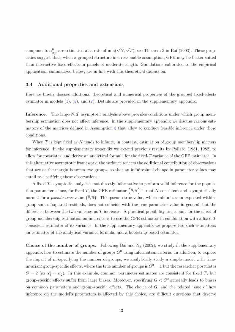
Coefficient estimates: income and lagged democracy. Figure 1 shows the point-estimates

and standard errors of income and lagged democracy coefficients for different values of the number of

groups G, on the 1970-2000 balanced subsample of Acemoglu et al. (2008).17 The right panel shows

that the implied cumulative income effect θ2/(1 − θ1) sharply decreases from .25 in OLS to .10 for

G = 5, and remains almost constant as G increases further. The left and middle panels show that

this pattern is mostly driven by a decrease in the coefficient of lagged democracy. This is consistent

with unobserved country heterogeneity being positively correlated with lagged democracy, causing an

upward bias in OLS.

Note that, though statistically significant, the cumulative income effect is quantitatively small.

Moreover, we show in the supplementary appendix that the association between income and democ-

racy disappears in a specification that combines both time-varying grouped effects and time-invariant

country-specific effects, as in model (5). Hence, in this specification which nests the one in Acemoglu

et al. (2008), the income effect is not statistically different from zero.

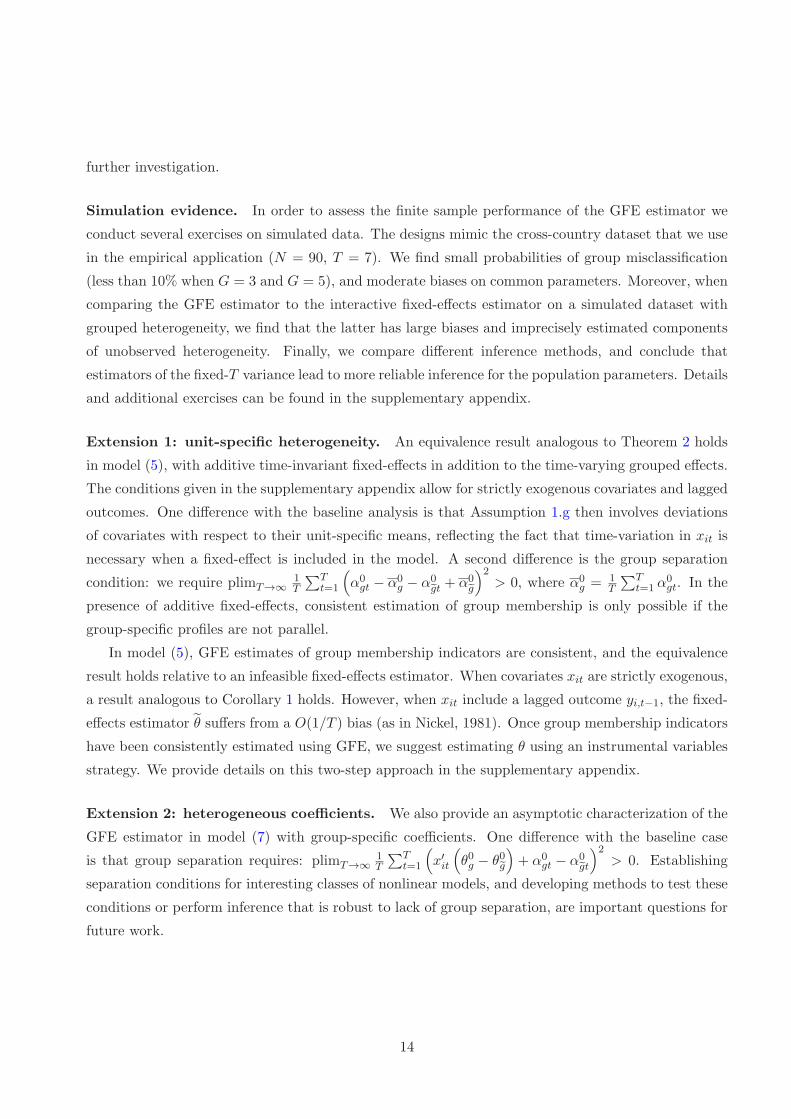
Grouped patterns. The GFE estimates of the unobserved determinants of democracy reveal het-

erogeneous, time-varying patterns. The upper panel of Figure 2 shows the estimates of group mem-

bership by country on a World map, when G = 4. The bottom panel shows the parameter estimates

16All data in this section are taken from the files of Acemoglu et al. (2008): http://economics.mit.edu/files/500017All estimates are computed using Algorithm 2. We performed extensive checks of numerical accuracy, some of which

are described in the supplementary appendix. Stata codes to replicate the results are available as supplementary material.

15

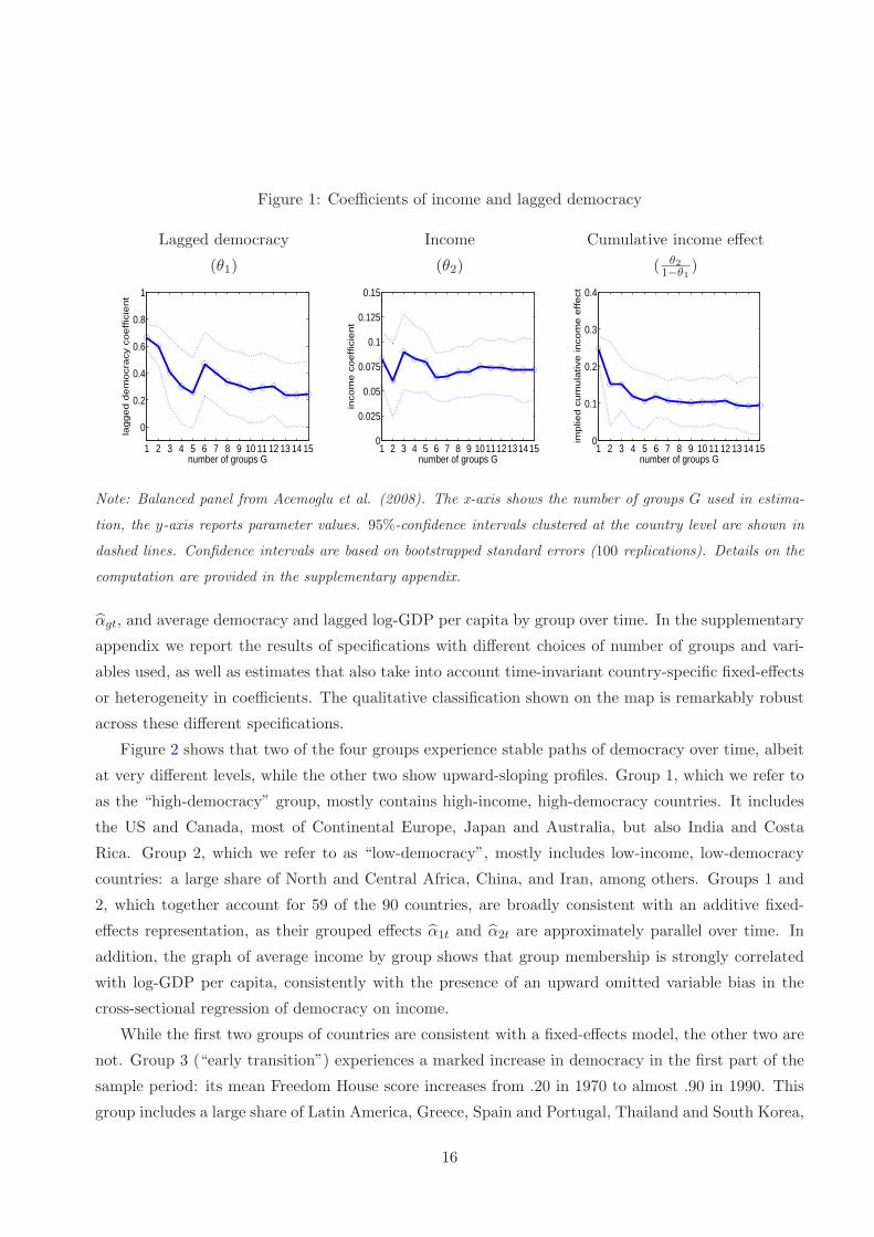
Figure 1: Coefficients of income and lagged democracy

Lagged democracy Income Cumulative income effect

(θ1) (θ2) ( θ21−θ1

)

1 2 3 4 5 6 7 8 9 10 11 12 13 14 15

0

0.2

0.4

0.6

0.8

1

number of groups G

lag

ge

d d

em

ocra

cy c

oe

ffic

ien

t

1 2 3 4 5 6 7 8 9 1011121314150

0.025

0.05

0.075

0.1

0.125

0.15

number of groups G

inco

me

co

effic

ien

t

1 2 3 4 5 6 7 8 9 10 11 12 13 14 150

0.1

0.2

0.3

0.4

number of groups G

imp

lied

cu

mu

lative

in

co

me

effe

ct

Note: Balanced panel from Acemoglu et al. (2008). The x-axis shows the number of groups G used in estima-

tion, the y-axis reports parameter values. 95%-confidence intervals clustered at the country level are shown in

dashed lines. Confidence intervals are based on bootstrapped standard errors (100 replications). Details on the

computation are provided in the supplementary appendix.

αgt, and average democracy and lagged log-GDP per capita by group over time. In the supplementary

appendix we report the results of specifications with different choices of number of groups and vari-

ables used, as well as estimates that also take into account time-invariant country-specific fixed-effects

or heterogeneity in coefficients. The qualitative classification shown on the map is remarkably robust

across these different specifications.

Figure 2 shows that two of the four groups experience stable paths of democracy over time, albeit

at very different levels, while the other two show upward-sloping profiles. Group 1, which we refer to

as the “high-democracy” group, mostly contains high-income, high-democracy countries. It includes

the US and Canada, most of Continental Europe, Japan and Australia, but also India and Costa

Rica. Group 2, which we refer to as “low-democracy”, mostly includes low-income, low-democracy

countries: a large share of North and Central Africa, China, and Iran, among others. Groups 1 and

2, which together account for 59 of the 90 countries, are broadly consistent with an additive fixed-

effects representation, as their grouped effects α1t and α2t are approximately parallel over time. In

addition, the graph of average income by group shows that group membership is strongly correlated

with log-GDP per capita, consistently with the presence of an upward omitted variable bias in the

cross-sectional regression of democracy on income.

While the first two groups of countries are consistent with a fixed-effects model, the other two are

not. Group 3 (“early transition”) experiences a marked increase in democracy in the first part of the

sample period: its mean Freedom House score increases from .20 in 1970 to almost .90 in 1990. This

group includes a large share of Latin America, Greece, Spain and Portugal, Thailand and South Korea,

16

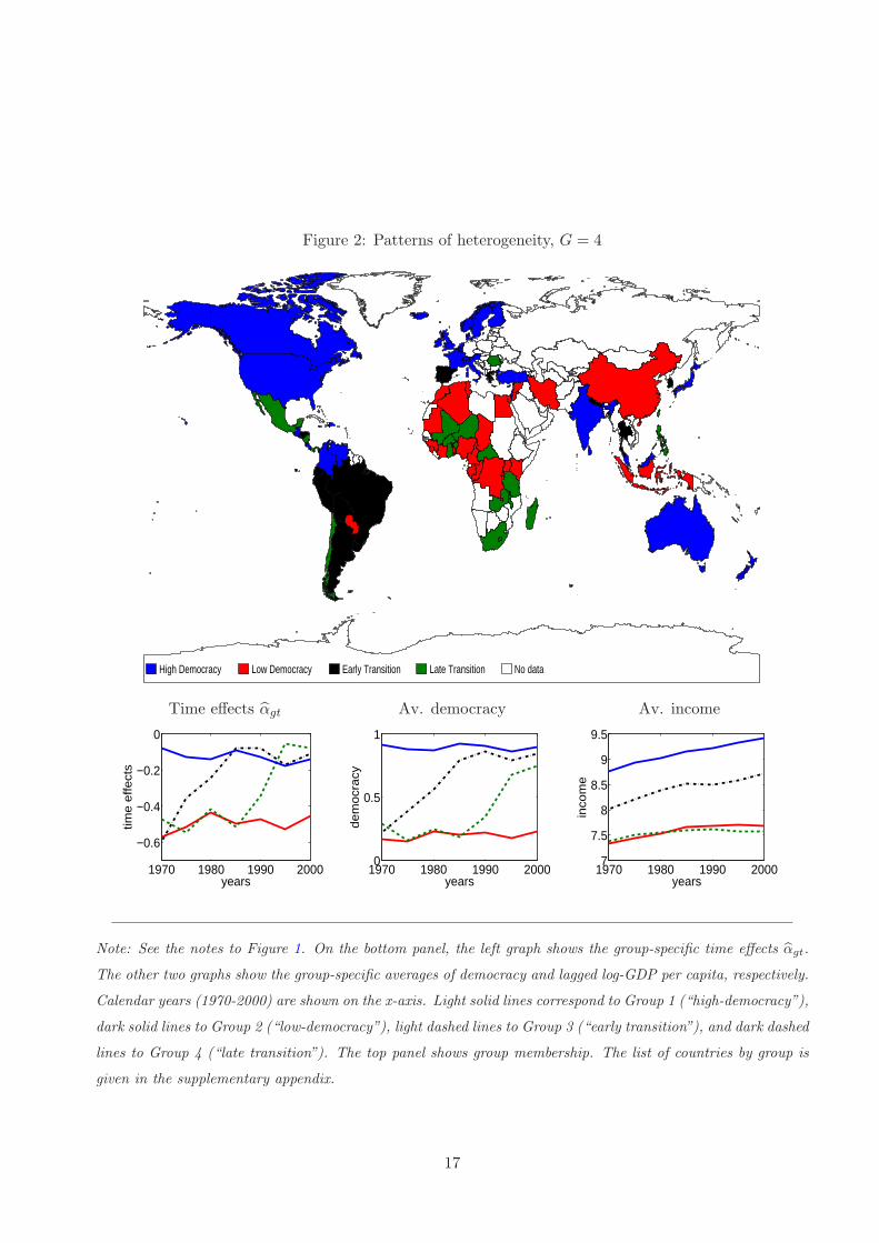
Figure 2: Patterns of heterogeneity, G = 4

High Democracy Low Democracy Early Transition Late Transition No data

Time effects αgt Av. democracy Av. income

1970 1980 1990 2000

−0.6

−0.4

−0.2

0

years

time

effe

cts

1970 1980 1990 20000

0.5

1

years

de

mo

cra

cy

1970 1980 1990 20007

7.5

8

8.5

9

9.5

years

inco

me

Note: See the notes to Figure 1. On the bottom panel, the left graph shows the group-specific time effects αgt.

The other two graphs show the group-specific averages of democracy and lagged log-GDP per capita, respectively.

Calendar years (1970-2000) are shown on the x-axis. Light solid lines correspond to Group 1 (“high-democracy”),

dark solid lines to Group 2 (“low-democracy”), light dashed lines to Group 3 (“early transition”), and dark dashed

lines to Group 4 (“late transition”). The top panel shows group membership. The list of countries by group is

given in the supplementary appendix.

17

in total 13 countries, with an intermediate level of GDP per capita. Group 4 (“late transition”) makes

a later transition to democracy: its average Freedom House score increases from .20 to .75 between

1985 and 2000. This group includes 18 countries, among which are a large part of West and South

Africa, Chile, Romania, and Philippines. These are low-income countries, whose GDP per capita is

similar on average to that of the “low-democracy” group (Group 2).

Note that the time patterns and group membership in Figure 2 are estimated from the panel data,

and not driven by modelling assumptions other than the grouped structure. In particular, nothing in

our framework imposes that time patterns are smooth over time. Moreover, group membership is not

assumed to have a particular spatial structure, so the geographic correlation apparent on the map is

purely a result of estimation.

Discussion. Overall, the evidence obtained suggests that the effect of income on democracy is

perhaps zero, or in any case quantitatively small, in line with the conclusions of Acemoglu et al.

(2008). At the same time, our analysis highlights the presence of clustering in the evolution of political

outcomes: while a substantial share of the world seems to have experienced stable parallel political

patterns during the period, roughly one third of the sample has experienced steep upward transitions.

These results raise interesting questions: which factors explain democratic transitions, and im-

portantly, why we observe groups of countries making transitions at similar points in time. In the

supplementary appendix we present a first attempt at explaining why these groups of countries have

evolved so differently, by regressing group membership on various determinants (including historical

measures). We see our framework as providing a starting point to assess how well different theories of

democratization fit the political and economic evolution of countries over time.

5 Conclusion

Grouped fixed-effects (GFE) offers a flexible yet parsimonious approach to model unobserved hetero-

geneity. The approach delivers estimates of common regression parameters, together with interpretable

estimates of group-specific time patterns and group membership. The framework allows for strictly

exogenous covariates and lagged outcomes. It also easily accommodates unit-specific fixed-effects in

addition to the time-varying grouped patterns, and grouped heterogeneity in coefficients. Importantly,

the relationship between group membership and observed covariates is left unrestricted.

The GFE approach should be useful in applications where time-varying grouped effects may be

present in the data. As a first example, the empirical analysis of the evolution of democracy shows

evidence of a clustering of political regimes and transitions. More generally, GFE should be well-

suited in difference-in-difference designs, as a way to relax parallel trend assumptions. Other potential

applications include models of social interactions and spatial dependence where the reference groups

or the spatial weights matrix are estimated from the panel data.

18

The extension to nonlinear models is a natural next step. While it is possible to define GFE esti-

mators in more general models (see for example equation (9)), the analysis raises statistical challenges.

One area of applications is static or dynamic discrete choice modelling, where a discrete specification

of unobserved heterogeneity may be appealing (Kasahara and Shimotsu, 2009, Browning and Carro,

2013). See Saggio (2012) for a first attempt in this direction.

Lastly, another interesting extension is to relax the assumption that there is a finite number of

well-separated groups in the population. As an alternative approach, one could view the grouped

model as an approximation to the underlying data generating process, and characterize the statistical

properties of GFE as the number of groups G increases with the two dimensions of the panel.

19

References

[1] Acemoglu, D., S. Johnson, J. Robinson, and P. Yared (2008): “Income and Democracy,” American

Economic Review, 98, 808–842.

[2] Ahlquist, J., and E. Wibbels (2012): “Riding the Wave: World Trade and Factor-Based Models

of Democratization,” to appear in American Journal of Political Science.

[3] Andrews, D. (1984): “Non-Strong Mixing Autoregressive Processes,” Journal of Applied Proba-

bility, 21, 930–934.

[4] Arellano, M., and J. Hahn (2007): “Understanding Bias in Nonlinear Panel Models: Some Recent

Developments,”. In: R. Blundell, W. Newey, and T. Persson (eds.): Advances in Economics and

Econometrics, Ninth World Congress, Cambridge University Press.

[5] Bai, J. (2003), “Inferential Theory for Factor Models of Large Dimensions,” Econometrica, 71,

135–171.

[6] Bai, J. (2009), “Panel Data Models with Interactive Fixed Effects,” Econometrica, 77, 1229–1279.

[7] Bai, J., and S. Ng (2002): “Determining the Number of Factors in Approximate Factor Models,”

Econometrica, 70, 191–221.

[8] Barro, R. J. (1999): “Determinants of Democracy,” Journal of Political Economy, 107(6), S158–

83.

[9] Bester, A., and C. Hansen (2013): “Grouped Effects Estimators in Fixed Effects Models”, to

appear in the Journal of Econometrics.

[10] Bickel, P.J., and A. Chen (2009): “A Nonparametric View of Network Models and Newman-

Girvan and Other Modularities,” Proc. Natl. Acad. Sci. USA, 106, 21068–21073.

[11] Blume, L.E., W.A. Brock, S.N. Durlauf, and Y.M. Ioannides (2011): “Identification of Social

Interactions,” in: J. Benhabib, A. Bisin, and M.O. Jackson (Eds.), Handbook of Social Economics,

Amsterdam: Elsevier Science.

[12] Browning, M., and J. Carro (2013): “Dynamic Binary Outcome Models with Maximal Hetero-

geneity”, to appear in the Journal of Econometrics.

[13] Bryant, P. and Williamson, J. A. (1978): “Asymptotic Behaviour of Classification Maximum

Likelihood Estimates,” Biometrika, 65, 273–281.

[14] Canova, F. (2004): “Testing for Convergence Clubs in Income per Capita: A Predictive Density

Approach,” International Economic Review, 45(1), 49–77.

20

[15] Choi, D.S., P.J. Wolfe, and E.M. Airoldi (2012): “Stochastic Blockmodels with a Growing Number

of Classes,” Biometrika, 99, 273–284.

[16] Forgy, E.W. (1965): “Cluster Analysis of Multivariate Data: Efficiency vs. Interpretability of

Classifications,” Biometrics, 21, 768–769.

[17] Fruhwirth-Schnatter, S. (2006): Finite Mixture and Markov Switching Models, Springer.

[18] Gleditsch, K.S., and M.D. Ward (2006): “Diffusion and the International Context of Democrati-

zation,” International Organization, 60, 911–933.

[19] Hahn, J., and H. Moon (2010): “Panel Data Models with Finite Number of Multiple Equilibria,”

Econometric Theory, 26(3), 863–881.

[20] Hansen, P., and N. Mladenovic (2001): “J-Means: A New Local Search Heuristic for Minimum

Sum-of-Squares Clustering,” Pattern Recognition, 34(2), 405–413.

[21] Hansen, P., N. Mladenovic, and J. A. Moreno Perez (2010): “Variable Neighborhood Search:

Algorithms and Applications,” Annals of Operations Research, 175, 367–407.

[22] Huntington, S.P. (1991): The Third Wave: Democratization in the Late Twentieth Century,

Norman, OK, and London: University of Oklahoma Press.

[23] Kasahara, H., and K. Shimotsu (2009): “Nonparametric Identification of Finite Mixture Models

of Dynamic Discrete Choices,” Econometrica, 77(1), 135–175.

[24] Lin, C. C., and S. Ng (2012): “Estimation of Panel Data Models with Parameter Heterogeneity

when Group Membership is Unknown”, Journal of Econometric Methods, 1(1), 42–55.

[25] Lipset, S. M. (1959): “Some Social Requisites of Democracy: Economic Development and Political

Legitimacy,” American Political Science Review, 53(1), 69–105.

[26] McLachlan, G., and D. Peel (2000): Finite Mixture Models, Wiley Series in Probabilities and

Statistics.

[27] Merlevede, F., Peligrad, M. and E. Rio (2011): “A Bernstein Type Inequality and Moderate

Deviations for Weakly Dependent Sequences,” Probability Theory and Related Fields, 151, 435–

474.

[28] Nickel, S. (1981): “Biases in Dynamic Models with Fixed Effects,” Econometrica, 49, 1417–1426.

[29] Phillips, P.C.B., and D. Sul (2007): “Transition Modelling and Econometric Convergence Tests,”

Econometrica, 75, 1771–1855.

21

[30] Pollard, D. (1981): “Strong Consistency of K-means Clustering,” Annals of Statistics, 9, 135–

140.

[31] Pollard, D. (1982): “A Central Limit Theorem for K-Means Clustering,” Annals of Probability,

10, 919–926.

[32] Rio, E. (2000): Theorie Asymptotique des Processus Aleatoires Faiblement Dependants, SMAI,

Springer.

[33] Saggio, R. (2012): “Discrete Unobserved Heterogeneity in Discrete Choice Panel Data Models,”

CEMFI Master Thesis.

[34] Sarafidis, V., and T. Wansbeek (2012): “Cross-sectional Dependence in Panel Data Analysis,” to

appear in Econometric Reviews.

[35] Steinley, D. (2006): “K-means Clustering: A Half-Century Synthesis,” Br. J. Math. Stat. Psychol.,

59, 1–34.

[36] Stock, J., and M. Watson (2002): “Forecasting Using Principal Components from a Large Number

of Predictors,” Journal of the American Statistical Association, 97, 1167–1179.

[37] Sun, Y. (2005): “Estimation and Inference in Panel Structure Models,” unpublished manuscript.

[38] Tibshirani, R. (1996): “Regression Shrinkage and Selection via the Lasso,” J. Roy. Statist. Soc.

Ser. B, 58, 267–288.

[39] Townsend, R. M. (1994): “Risk and Insurance in Village India,” Econometrica, 62, 539–91.

22

APPENDIX

A Proof of Theorem 1

Let γ0 = g01 , ..., g0N denote the population grouping. Let also γ = g1, ..., gN denote any grouping of the

cross-sectional units into G groups. Let us define:

Q (θ, α, γ) =1

NT

N∑

i=1

T∑

t=1

(yit − x′itθ − αgit)2. (A1)

Note that the GFE estimator minimizes Q (·) over all (θ, α, γ) ∈ Θ×AGT × ΓG. Note also that:

Q (θ, α, γ) =1

NT

N∑

i=1

T∑

t=1

(vit + x′it

(θ0 − θ

)+ α0

g0i t− αgit

)2.

We also define the following auxiliary objective function:

Q (θ, α, γ) =1

NT

N∑

i=1

T∑

t=1

(x′it(θ0 − θ

)+ α0

g0i t− αgit

)2+

1

NT

N∑

i=1

T∑

t=1

v2it.

We start by showing the following uniform convergence result.

Lemma A1 Let Assumption 1.a-1.f hold. Then:

plimN,T→∞

sup(θ,α,γ)∈Θ×AGT×ΓG

∣∣∣Q (θ, α, γ)− Q (θ, α, γ)∣∣∣ = 0.

Proof.

Q (θ, α, γ)− Q (θ, α, γ) =2

NT

N∑

i=1

T∑

t=1

vit

(x′it(θ0 − θ

)+ α0

g0i t− αgit

)

=

(2

NT

N∑

i=1

T∑

t=1

vitxit

)′ (θ0 − θ

)+

2

NT

N∑

i=1

T∑

t=1

vitα0g0i t− 2

NT

N∑

i=1

T∑

t=1

vitαgit.

By Assumption 1.d we have:

E

1

N

N∑

i=1

∥∥∥∥∥1

T

T∑

t=1

vitxit

∥∥∥∥∥

2 ≤ M

T,

so it follows from the Cauchy-Schwartz (CS) inequality that 2NT

∑Ni=1

∑Tt=1 vitxit = op(1). In addition,

∥∥θ0 − θ∥∥

is bounded by Assumption 1.a.

We next show that 1NT

∑Ni=1

∑Tt=1 vitαgit is op(1), uniformly on the parameter space. This will imply that

1NT

∑Ni=1

∑Tt=1 vitα

0g0i t

= op(1). We have:

1

NT

N∑

i=1

T∑

t=1

vitαgit =G∑

g=1

[1

NT

N∑

i=1

T∑

t=1

1gi = gvitαgt

]=

G∑

g=1

[1

T

T∑

t=1

αgt

(1

N

N∑

i=1

1gi = gvit)]

.

Moreover, by the CS inequality and for all g ∈ 1, ..., G:(

1

T

T∑

t=1

αgt

(1

N

N∑

i=1

1gi = gvit))2

≤(

1

T

T∑

t=1

α2gt

)×

1

T

T∑

t=1

(1

N

N∑

i=1

1gi = gvit)2 ,

23

where, by Assumption 1.a, 1T

∑Tt=1 α

2gt is uniformly bounded. Now, note that:

1

T

T∑

t=1

(1

N

N∑

i=1

1gi = gvit)2

=1

TN2

N∑

i=1

N∑

j=1

1gi = g1gj = gT∑

t=1

vitvjt ≤ 1

N2

N∑

i=1

N∑

j=1

∣∣∣∣∣1

T

T∑

t=1

vitvjt

∣∣∣∣∣

≤ 1

N2

N∑

i=1

N∑

j=1

∣∣∣∣∣1

T

T∑

t=1

E (vitvjt)

∣∣∣∣∣+1

N2

N∑

i=1

N∑

j=1

∣∣∣∣∣1

T

T∑

t=1

(vitvjt − E (vitvjt))

∣∣∣∣∣ .

By Assumption 1.e: 1N2

∑Ni=1

∑Nj=1

∣∣∣ 1T∑T

t=1 E (vitvjt)∣∣∣ ≤ M

N. Moreover, by the CS inequality:

1

N2

N∑

i=1

N∑

j=1

∣∣∣∣∣1

T

T∑

t=1

(vitvjt − E (vitvjt))

∣∣∣∣∣

2

≤ 1

N2

N∑

i=1

N∑

j=1

(1

T

T∑

t=1

(vitvjt − E (vitvjt))

)2

,

which is bounded in expectation by M/T by Assumption 1.f.

This shows that 1NT

∑Ni=1

∑Tt=1 vitαgit is uniformly op(1), and ends the proof of Lemma A1.

The following result shows that Q (·) is uniquely minimized at true values.

Lemma A2 For all (θ, α, γ) ∈ Θ×AGT × ΓG:

Q (θ, α, γ)− Q(θ0, α0, γ0

)≥ ρ

∥∥θ − θ0∥∥2 ,

where ρ is given by Assumption 1.g.

Proof. Let us denote, for every grouping γ = g1, ..., gN:

Σ (γ) =1

NT

N∑

i=1

T∑

t=1

(xit − xg0

i∧gi,t

)(xit − xg0

i∧gi,t

)′.

We have, using standard least-squares algebra:

Q (θ, α, γ)− Q(θ0, α0, γ0

)=

1

NT

N∑

i=1

T∑

t=1

(x′it(θ0 − θ

)+ α0

g0i t− αgit

)2≥(θ0 − θ

)′Σ(γ)

(θ0 − θ

)

≥ minγ∈ΓG

(θ0 − θ

)′Σ(γ)

(θ0 − θ

)≥(minγ∈ΓG

ρ(γ)

)∥∥θ0 − θ∥∥2 ,

where minγ∈ΓGρ(γ) is asymptotically bounded away from zero by Assumption 1.g.

To show that θ is consistent for θ0, note that, by Lemma A1 and by the definition of the GFE estimator:

Q(θ, α, γ

)= Q

(θ, α, γ

)+ op(1) ≤ Q

(θ0, α0, γ0

)+ op(1) = Q

(θ0, α0, γ0

)+ op(1). (A2)

So, by Lemma A2 and Assumption 1.g:∥∥∥θ − θ0

∥∥∥2

= op(1).

Lastly, to show convergence in quadratic mean of the estimated unit-specific effects, note that:

∣∣∣Q(θ, α, γ

)− Q

(θ0, α, γ

)∣∣∣ =

∣∣∣∣∣1

NT

N∑

i=1

T∑

t=1

x′it(θ0 − θ

) [x′it(θ0 − θ

)+ 2

(α0g0i t− αgit

)]∣∣∣∣∣

≤ 1

NT

N∑

i=1

T∑

t=1

‖xit‖2 ×∥∥∥θ0 − θ

∥∥∥2

+

(4 supαt∈A

|αt|)× 1

NT

N∑

i=1

T∑

t=1

‖xit‖ ×∥∥∥θ0 − θ

∥∥∥ ,

24

which is op(1) by Assumptions 1.a and 1.b, and by consistency of θ. Combining with (A2) we obtain:

Q(θ0, α, γ

)≤ Q

(θ0, α0, γ0

)+ op(1), from which it follows that: 1

NT

∑Ni=1

∑Tt=1

(αgit − α0

g0i t

)2= op(1).

This completes the proof of Theorem 1.

B Proof of Theorem 2

We first establish that α is consistent for α0. Because the objective function is invariant to re-labelling of the

groups, we show consistency with respect to the Hausdorff distance dH in RGT , defined by:

dH (a, b)2= max

max

g∈1,...,G

(min

g∈1,...,G

1

T

T∑

t=1

(agt − bgt)2

), maxg∈1,...,G

(min

g∈1,...,G

1

T

T∑

t=1

(agt − bgt)2

).

We have the following result.18

Lemma B3 Let Assumptions 1.a-1.g, and 2.a-2.b hold. Then, as N and T tend to infinity:

dH(α, α0

) p→ 0.

Proof.

We study the two terms in the max·, · in turn.

• We first show that, for all g ∈ 1, ..., G:

ming∈1,...,G

1

T

T∑

t=1

(αgt − α0

gt

)2 p→ 0. (B3)

Let g ∈ 1, ..., G. We have:

1

NT

N∑

i=1

(min

g∈1,...,G

T∑

t=1

1g0i = g(αgt − α0

gt

)2)

=

(1

N

N∑

i=1

1g0i = g)(

ming∈1,...,G

1

T

T∑

t=1

(αgt − α0

gt

)2).

By Assumption 2.a it is thus enough to show that, for all g, as N and T tend to infinity:

1

NT

N∑

i=1

(min

g∈1,...,G

T∑

t=1

1g0i = g(αgt − α0

gt

)2)

p→ 0.

Now:

1

NT

N∑

i=1

1g0i = g(

ming∈1,...,G

T∑

t=1

(αgt − α0

gt

)2)

≤ 1

NT

N∑

i=1

1g0i = g(

T∑

t=1

(αgit − α0

gt

)2)

≤ 1

NT

N∑

i=1

T∑

t=1

(αgit − α0

g0i t

)2,

which is op(1) by Theorem 1. Hence (B3) follows.

• Let us define, for all g ∈ 1, ..., G:

σ(g) = argming∈1,...,G

1

T

T∑

t=1

(αgt − α0

gt

)2.

18Note that group separation (Assumption 2.b) is assumed to show Lemma B3. Proving consistency of the group-

specific time effects absent this assumption would require different arguments.

25

We start by showing that σ : 1, ..., G → 1, ..., G is one-to-one, with probability approaching one as T

tends to infinity. Let g 6= g. By the triangle inequality we have:

(1

T

T∑

t=1

(ασ(g)t − ασ(g)t

)2) 1

2

≥(

1

T

T∑

t=1

(α0gt − α0

gt

)2) 1

2

−(

1

T

T∑

t=1

(ασ(g)t − α0

gt

)2) 1

2

−(

1

T

T∑

t=1

(ασ(g)t − α0

gt

)2) 1

2

,

where the right-hand-side of this inequality converges in probability to (cg,g)12 by Assumption 2.b and equation

(B3). It thus follows that, with probability approaching one, σ(g) 6= σ(g) for all g 6= g. Thus σ admits a

well-defined inverse σ−1.

Now, with probability approaching one we have, for all g ∈ 1, ..., G:

ming∈1,...,G

1

T

T∑

t=1

(αgt − α0

gt

)2 ≤ 1

T

T∑

t=1

(αgt − α0

σ−1(g)t

)2= min

h∈1,...,G1

T

T∑

t=1

(αht − α0

σ−1(g)t

)2 p→ 0,

where we have used (B3), and the fact that g = σ[σ−1 (g)

]. Combining with (B3) completes the proof.

The proof of Lemma B3 shows that there exists a permutation σ : 1, ..., G → 1, ..., G such that:

1

T

T∑

t=1

(ασ(g)t − α0

gt

)2 p→ 0.

By simple relabelling of the elements of α we may take σ(g) = g. We adopt this convention in the rest of the

proof. For any η > 0, we let Nη denote the set of parameters (θ, α) ∈ Θ×AGT that satisfy∥∥θ − θ0

∥∥2 < η and1T

∑Tt=1

(αgt − α0

gt

)2< η for all g ∈ 1, ..., G. We have the following result.

Lemma B4 For η > 0 small enough we have, for all δ > 0 and as N and T tend to infinity:

sup(θ,α)∈Nη

1

N

N∑

i=1

1gi (θ, α) 6= g0i = op(T−δ

).

Proof.

Note that, from the definition of gi(·) we have, for all g ∈ 1, ..., G:

1 gi (θ, α) = g ≤ 1

T∑

t=1

(yit − x′itθ − αgt)2 ≤

T∑

t=1

(yit − x′itθ − αg0

i t

)2,

so:

1

N

N∑

i=1

1gi (θ, α) 6= g0i

=

G∑

g=1

1

N

N∑

i=1

1g0i 6= g

1 gi (θ, α) = g

≤G∑

g=1

1

N

N∑

i=1

1g0i 6= g1

T∑

t=1

(yit − x′itθ − αgt)2 ≤

T∑

t=1

(yit − x′itθ − αg0

i t

)2

︸ ︷︷ ︸=Zig(θ,α)

.

We start by bounding Zig(θ, α), for all (θ, α) ∈ Nη, by a quantity that does not depend on (θ, α). To

proceed note that, for all (θ, α) and all i:

Zig(θ, α) = 1g0i 6= g1

T∑

t=1

(αg0

i t− αgt

)(vit + x′it

(θ0 − θ

)+ α0

g0i t−αgt + αg0

i t

2

)≤ 0

≤ maxg 6=g

1

T∑

t=1

(αgt − αgt)

(vit + x′it

(θ0 − θ

)+ α0

gt −αgt + αgt

2

)≤ 0

.

26

Let us now define:

AT =

∣∣∣∣∣T∑

t=1

(αgt − αgt)

(vit + x′it

(θ0 − θ

)+ α0

gt −αgt + αgt

2

)−

T∑

t=1

(α0gt − α0

gt

)(vit + α0

gt −α0gt + α0

gt

2

)∣∣∣∣∣ .

As we have:

AT ≤∣∣∣∣∣

T∑

t=1

(αgt − αgt) vit −T∑

t=1

(α0gt − α0

gt

)vit

∣∣∣∣∣+∣∣∣∣∣

T∑

t=1

(αgt − αgt)x′it

(θ0 − θ

)∣∣∣∣∣

+

∣∣∣∣∣T∑

t=1

(αgt − αgt)

(α0gt −

αgt + αgt

2

)−

T∑

t=1

(α0gt − α0

gt

)(α0gt −

α0gt + α0

gt

2

)∣∣∣∣∣ ,

it is easy to show using the CS inequality that, for (θ, α) ∈ Nη:

AT ≤ TC1√η

(1

T

T∑

t=1

v2it

) 12

+ TC2√η

(1

T

T∑

t=1

‖xit‖)

+ TC3√η,

where C1, C2 and C3 are constants, independent of η and T .

We thus obtain that:

Zig(θ, α) ≤ maxg 6=g

1

T∑

t=1

(α0gt − α0

gt

)(vit + α0

gt −α0gt + α0

gt

2

)

≤ TC1√η

(1

T

T∑

t=1

v2it

) 12

+ TC2√η

(1

T

T∑

t=1

‖xit‖)

+ TC3√η

.

Noting that the right-hand side of this inequality does not depend on (θ, α), it follows that: sup(θ,α)∈NηZig(θ, α) ≤

Zig, where:

Zig = maxg 6=g

1

T∑

t=1

(α0gt − α0

gt

)vit ≤ −1

2

T∑

t=1

(α0gt − α0

gt

)2+ TC1

√η

(1

T

T∑

t=1

v2it

) 12

+TC2√η

(1

T

T∑

t=1

‖xit‖)

+ TC3√η

. (B4)

As a result:

sup(θ,α)∈Nη

1

N

N∑

i=1

1gi (θ, α) 6= g0i ≤ 1

N

N∑

i=1

G∑

g=1

Zig. (B5)

Fix M > max(√M,M∗), where M and M∗ are given by Assumptions 1 and 2.e, respectively. Note that

E(v2it) ≤√M . We have, using standard probability algebra and for all g:

Pr(Zig = 1

)≤

∑

g 6=g

Pr

(T∑

t=1

(α0gt − α0

gt

)vit ≤ −1

2

T∑

t=1

(α0gt − α0

gt

)2+ TC1

√η

(1

T

T∑

t=1

v2it

) 12

+TC2√η

(1

T

T∑

t=1

‖xit‖)

+ TC3√η

)

≤∑

g 6=g

[Pr

(1

T

T∑

t=1

‖xit‖ ≥ M

)+ Pr

(1

T

T∑

t=1

(α0gt − α0

gt

)2 ≤ cg,g2

)+ Pr

(1

T

T∑

t=1

v2it ≥ M

)

+Pr

(T∑

t=1

(α0gt − α0

gt

)vit ≤ −T cg,g

4+ TC1

√η√M + TC2

√ηM + TC3

√η

)].

(B6)

27

To end the proof of Lemma B4, we rely on the use of exponential inequalities for dependent processes.

Specifically, we use the following result, which is a direct consequence of Theorem 6.2 in Rio (2000).

Lemma B5 Let zt be a strongly mixing process with zero mean, with strong mixing coefficients α[t] ≤ e−atd1 ,

and with tail probabilities Pr(|zt| > z) ≤ e1−(zb )

d2

, where a, b, d1, and d2 are positive constants. Then, for all

z > 0 we have, for all δ > 0:

T δ Pr

(∣∣∣∣∣1

T

T∑

t=1

zt

∣∣∣∣∣ ≥ z

)T→∞→ 0.

Proof. Let s2 = supt≥1

(∑s≥1 |E (ztzs)|

). Note that s2 < ∞ under the condition of Lemma B5.19 Let also

d = d1d2

d1+d2. By evaluating inequality (1.7) in Merlevede et al. (2011) at λ = T z

4 and r = T12 , we obtain that

there exists a constant f > 0 independent of T such that, for all z > 0 and T ≥ 1:

Pr

(∣∣∣∣∣1

T

T∑

t=1

zt

∣∣∣∣∣ ≥ z

)≤ 4

(1 + T

12z2

16s2

)− 12T

12

+16f

zexp

(−a(T

12z

4b

)d).

Lemma B5 directly follows.

We now bound the last three terms on the right-hand side of (B6).

• By Assumptions 1.a and 2.b we have limT→∞ 1T

∑Tt=1 E

[(α0gt − α0

gt

)2]= cg,g. So for T large enough we

have:

1

T

T∑

t=1

E

[(α0gt − α0

gt

)2] ≥ 2cg,g3

.

Applying Lemma B5 to zt =(α0gt − α0

gt

)2− E

[(α0gt − α0

gt

)2], which satisfies appropriate mixing and tail

conditions by Assumptions 1.a and 2.c, and taking z =cg,g6 yields, for all δ > 0 and as T tends to infinity:

Pr

(1

T

T∑

t=1

(α0gt − α0

gt

)2 ≤ cg,g2

)= o

(T−δ

).

• Similarly, for the third term on the right-hand side of (B6), applying Lemma B5 to zt = v2it − E(v2it) and

taking z = M −√M yields:

Pr

(1

T

T∑

t=1

v2it ≥ M

)= o

(T−δ

)

for all δ > 0. Note that v2itt is strongly mixing as vitt is strongly mixing by Assumption 2.c.

• Lastly, to bound the fourth term on the right-hand side of (B6) we denote as c the minimum of cg,g over

all g 6= g and we take:

η ≤

c

8(C1

√M + C2M + C3

)

2

. (B7)

Note that this upper bound on η does not depend on T .

19This is a consequence of the fact that |Cov(X,Y )| can be bounded in terms of the strong mixing coefficient α[X,Y ]

and the quantile functions QX and QY (see, e.g., Theorem 1.1 in Rio, 2000).

28

Taking η satisfying (B7) yields, for all g 6= g:

Pr

(1

T

T∑

t=1

(α0gt − α0

gt

)vit ≤ −cg,g

4+ C1

√η√M + C2

√ηM + C3

√η

)≤ Pr

(1

T

T∑

t=1

(α0gt − α0

gt

)vit ≤ −cg,g

8

).

Now, by Assumption 2.c the process(α0gt − α0

gt

)vit

thas zero mean, and is strongly mixing with faster-

than-polynomial decay rate. Moreover, for all i, t, and m > 0:

Pr(∣∣(α0

gt − α0gt

)vit∣∣ > m

)≤ Pr

|vit| >

m

2 supαt∈A

|αt|

,

so(α0gt − α0

gt

)vit

talso satisfies the tail condition of Assumption 2.d, albeit with a different constant b > 0

instead of b > 0.

Lastly, applying Lemma B5 with zt =(α0gt − α0

gt

)vit and taking z =

cg,g8 yields:

Pr

(1

T

T∑

t=1

(α0gt − α0

gt

)vit ≤ −cg,g

8

)= o

(T−δ

). (B8)

Note that the above upper bounds on the probabilities do not depend on i and g. Combining results we

thus obtain, using (B6) and Assumption 2.e, that for η satisfying (B7) and for all δ > 0:

1

N

N∑

i=1

G∑

g=1

Pr(Zig = 1

)≤ G(G− 1) sup

i∈1,..,NPr

(1

T

T∑

t=1

‖xit‖ ≥ M

)+ o

(T−δ

)= o

(T−δ

). (B9)

Sufficient conditions for Assumption 2.e are given at the end of Appendix B.

To complete the proof of Lemma B4 note that, for η that satisfies (B7) we have, for all δ > 0 and all ε > 0:

Pr

(sup

(θ,α)∈Nη

1

N

N∑

i=1

1gi (θ, α) 6= g0i > εT−δ

)≤ Pr

(1

N

N∑

i=1

G∑

g=1

Zig > εT−δ

)≤

E

(1N

∑Ni=1

∑Gg=1 Zig

)

εT−δ= o(1),

where we have used (B5), the Markov inequality, and (B9), respectively.

This ends the proof of Lemma B4.

We now prove the three parts of Theorem 2, and derive asymptotic results for θ, α, and gi in turn.

Properties of θ. Let us denote:20

Q (θ, α) =1

NT

N∑

i=1

T∑

t=1

(yit − x′itθ − αgi(θ,α)t

)2, (B10)

and:

Q (θ, α) =1

NT

N∑

i=1

T∑

t=1

(yit − x′itθ − αg0

i t

)2. (B11)

Note that Q(·) is minimized at(θ, α

), and that Q(·) is minimized at

(θ, α

).

20Note that Q (θ, α) is a concentrated version of Q (θ, α, γ) that was defined in the proof of Theorem 1.

29

Let η > 0 be small enough such that Lemma B4 is satisfied. Using Assumptions 1.a-1.c and Lemma B4 it

is easy to see that, for all δ > 0:

sup(θ,α)∈Nη

∣∣∣Q (θ, α)− Q (θ, α)∣∣∣ = op

(T−δ

). (B12)

Now, by consistency of θ (Theorem 1) and α (Lemma B3) we have, as N and T tend to infinity:

Pr((θ, α

)/∈ Nη

)→ 0. (B13)

Likewise, as θ and α are also consistent under the conditions of Theorem 1 we have:

Pr((θ, α

)/∈ Nη

)→ 0. (B14)

Combining (B12) and (B13) we have, for all δ > 0 and as N and T tend to infinity:

Q(θ, α

)− Q

(θ, α

)= op

(T−δ

). (B15)

This is because, for every ε > 0:

Pr[∣∣∣Q

(θ, α

)− Q

(θ, α

)∣∣∣ > εT−δ]

≤ Pr((θ, α

)/∈ Nη

)+ Pr

[sup

(θ,α)∈Nη

∣∣∣Q (θ, α)− Q (θ, α)∣∣∣ > εT−δ

],

which is o(1) by (B12) and (B13).

Similarly, combining (B12) and (B14) we obtain:

Q(θ, α

)− Q

(θ, α

)= op

(T−δ

). (B16)

Hence, using (B15), (B16), and the definition of(θ, α

)and

(θ, α

)yields:

0 ≤ Q(θ, α

)− Q

(θ, α

)= Q

(θ, α

)− Q

(θ, α

)+ op(T

−δ) ≤ op(T−δ

).

It thus follows that:

Q(θ, α

)− Q

(θ, α

)= op

(T−δ

). (B17)

Now, using that(θ, α

)is a least squares estimator, we obtain:

Q(θ, α

)− Q

(θ, α

)=

1

NT

N∑

i=1

T∑

t=1

(x′it(θ − θ

)+ αg0

i t− αg0

i t

)2(B18)

≥(θ − θ

)′(

1

NT

N∑

i=1

T∑

t=1

(xit − xg0

i t

)(xit − xg0

i t

)′)(

θ − θ)

≥ ρ∥∥∥θ − θ

∥∥∥2

,

where ρp→ ρ > 0 as a consequence of Assumption 1.g. Hence, θ − θ = op

(T−δ

)for all δ > 0. This shows (17).

Properties of α. Using (B17) and (B18) above, consistency of θ and θ, and Assumption 1.b, we obtain:

1

NT

G∑

g=1

N∑

i=1

1g0i = gT∑

t=1

(αgt − αgt)2=

1

NT

N∑

i=1

T∑

t=1

(αg0

i t− αg0

i t

)2= op

(T−δ

).

Using Assumption 2.a, we thus have for all g:

1

T

T∑

t=1

(αgt − αgt)2

= op(T−δ

). (B19)

In particular, for all t we have: (αgt − αgt)2 ≤ op

(T 1−δ

). As this holds for all δ > 0 we obtain (18).

30

Properties of gi = gi

(θ, α

). Finally we have, by the union bound:

Pr

(sup

i∈1,...,N

∣∣∣gi(θ, α

)− g0i

∣∣∣ > 0

)≤ Pr

((θ, α

)/∈ Nη

)+N sup

i∈1,...,NPr((θ, α

)∈ Nη , gi

(θ, α

)6= g0i

).

Now we have, taking η such that (B7) is satisfied: Pr((θ, α

)/∈ Nη

)= o(1). Moreover, by the proof of

Lemma B4 we have: sup(θ,α)∈Nη1gi (θ, α) 6= g0i ≤∑G

g=1 Zig, where Zig is given by (B4). Hence:

N supi∈1,...,N

Pr((θ, α

)∈ Nη, gi

(θ, α

)6= g0i

)= N sup

i∈1,...,NE

[1(θ, α

)∈ Nη

1gi

(θ, α

)6= g0i

]

≤ N supi∈1,...,N

E

[1(θ, α

)∈ Nη

G∑

g=1

Zig

]

≤ N supi∈1,...,N

G∑

g=1

Pr(Zig = 1

)= o

(NT−δ

)for all δ > 0,

where the last equality is obtained similarly as (B9) under Assumption 2.e.

This implies (16), and completes the proof of Theorem 2.

Sufficient conditions for Assumption 2.e. We have the following result.

Proposition B1 Suppose that either of the following two conditions holds:

1. Assumption 1.b holds, and ‖xit‖t satisfies the mixing and tail conditions of Assumptions 2.c and 2.d.

2. Assumptions 1.a, 1.c, and 2.c-2.d, hold. Moreover, xit = (yi,t−1, x′it)

′, and θ =

(ρ, θ′1

)′, where |ρ0| < 1,

xit satisfy Assumption 2.e, and, for all constants F > 0:

supi∈1,..,N

Pr (|yi0| ≥ FT ) = o(T−δ

)for all δ > 0. (B20)

Note that (B20) requires that the distribution of yi0 has thinner-than-polynomial tails.

Then there exists a constant M∗ > 0 such that, as N,T tend to infinity:

supi∈1,..,N

Pr

(1

T

T∑

t=1

‖xit‖ ≥M∗)

= o(T−δ

)for all δ > 0.

Proof.

Let us first suppose Part 1. Note that E(‖xit‖) ≤√M by Assumption 1.b. Let M∗ >

√M . The result

comes from applying Lemma B5 to zt = ‖xit‖ − E(‖xit‖) and taking z =M∗ −√M .

Let us then suppose Part 2. By assumption, supi∈1,..,N Pr(

1T

∑Tt=1 ‖xit‖ ≥M∗

)= o

(T−δ

). Moreover:

yit =

t−1∑

s=0

(ρ0)s (

x′i,t−sθ01 + α0

g0i ,t−s + vi,t−s

)+(ρ0)tyi0.

So, for all i:

1

T

T∑

t=1

|yi,t−1| ≤ 1

T

T∑

t=1

[ t−2∑

s=0

(∣∣ρ0∣∣s(‖xi,t−1−s‖

∥∥θ01∥∥+

∣∣∣α0g0i ,t−1−s

∣∣∣+ |vi,t−1−s|))

+∣∣ρ0∣∣t−1 |yi0|

]

≤(

1

1− |ρ0|

)[ 1T

T−1∑

m=1

(‖xim‖

∥∥θ01∥∥+

∣∣∣α0g0im

∣∣∣+ |vim|)+

1

T|yi0|

],

31

where we have used the change-in-variables m = t− 1− s. Taking M∗ large enough, Assumptions 1.a, 1.c, 2.c,

2.d, and Lemma B5 imply that:

supi∈1,..,N

Pr

(1

T

T−1∑

m=1

(‖xim‖

∥∥θ01∥∥+

∣∣∣α0g0im

∣∣∣+ |vim|)≥ M∗(1−

∣∣ρ0∣∣)

2

)= o(T−δ).

Moreover, for this M∗, (B20) implies that:

supi∈1,..,N

Pr

(1

T|yi0| ≥

M∗(1−∣∣ρ0∣∣)

2

)= o(T−δ).

This concludes the proof.

32