Group replacement policies for parallel systems whose ...popova/phase.pdfIn this paper, a system of stochastically independent and identical components is analyzed. Group replacement

© J.C. Baltzer AG, Science Publishers

Group replacement policies for parallel systems whosecomponents have phase distributed failure times★

Elmira Popovaa and John G. Wilsonb

aGraduate Program in Operations Research and Industrial Enginering,Department of Mechanical Engineering, The University of Texas at Austin,

Austin, TX 78712, USA

E-mail: [email protected]

bThe Richard Ivey School of Business, The University of Western Ontario,London, Ontario, Canada N6A 3K7

Consider a system of components operating in parallel. Downtime costs are incurredwhen failed components are not repaired or replaced. There are also fixed, unit repair andreplacement costs associated with the system. The failure distributions of the componentsare assumed to be identically distributed random variables. Results on calculating the expectedcost and variance per unit time of various group replacement policies will be provided.Consideration of variance is important since, in many cases, practitioners wish not only toachieve small expected cost but also to reduce variability from cycle to cycle. Phase distri-butions allow for the modeling of a wide range failure time behavior. Closed-form resultsare derived for the three major classes of group replacement policy (m-failure, T-age, and(m, T)) when the underlying distribution is of phase type.

Keywords: maintenance, phase distributions, production planning, cost variability

AMS subject classification: Primary 90B25; Secondary 60K20, 62N05

1. Introduction

Over the past few decades, the complexity of industrial systems has grown enor-mously. New industrial paradigms to ensure fast production, delivery, and profit havebeen introduced. Just-in-time systems are among the most popular. Proper planningof maintenance is important to minimize disruptions to the system. The literature onreliability and maintainability of complex systems has evolved at a relatively slowpace due to the mathematical complexity of such problems and limited computationalcapabilities in the past.

★ This research has been partially supported by Grant #0003658-472 from the State of Texas AdvancedTechnology Program, National Science Foundation Grant #DMC-8910378, and a Babcock Research Grant.

Annals of Operations Research 91(1999)163–189 163

In this paper, a system of stochastically independent and identical components isanalyzed. Group replacement policies are investigated in detail. Group replacementpolicies require the replacement or repair to as good as new of all components when-ever any replacement or maintenance is performed. Their great advantages are thatthey allow for economies of scale and are straightforward to implement.

There are three main classes of group replacement policy. A T-age policy (see,e.g., Okumoto and Elsayed [11]) calls for replacement every T units of time. An m-failure policy (see, e.g., Assaf and Shanthikumar [1] and Wilson and Benmerzouga[17]) calls for replacing the system at the time of the m th failure. A policy that com-bines features of both of the above classes is the (m, T ) policy, which calls for replace-ment at the time of the m th failure or at time T whichever occurs first (see Ritchkenand Wilson [13] and Nakagawa [8]).

The work referenced above assumes that the parameters of the underlying failuretime distributions are known with certainty. In practice, an engineer’s opinion of thefailure time distributions will change as data from the actual operation of the systemis obtained. There have been a number of recent results on adaptive Bayesian ap-proaches to modeling this situation. For the case of exponential failure times, Wilsonand Benmerzouga [18] analyzed a policy class that called for replacement of thesystem whenever the expected posterior value of the exponential parameter exceededa certain threshold. A more general form of this policy for the case of three machinesoperating in parallel was considered in Wilson and Popova [19]. The case of a singlemachine with a Weibull failure time is considered in Mazzuchi and Soyer [7].

Group replacement policies are popular in large part due to the ease with whichthey can be implemented in a real production setting. There has been little work in theliterature on identifying which class of policies contains the optimal policy for a givensystem. For a parallel system where the components have exponential i.i.d. failuretimes, Assaf and Shanthikumar [1] showed that the class of m-failure policies is opti-mal if one knows the value of the underlying exponential parameter. Wilson andPopova [20] provide optimality results for the adaptive Bayesian case where theparameter is continuously estimated from the failure time data. The case where thesystem consists of only one component, but where the failure distribution is allowedto be any continuous distribution whose parameters are continuously updated, is con-sidered in Popova and Wilson [12].

All of the above approaches assume that one is only interested in finding a policythat minimizes the expected cost per unit time. However, many managers and engi-neers are often just as interested in the variability of cost from cycle to cycle. Indeed,many might prefer a policy with a slightly higher expected cost per unit time if thevariability of these costs is small. In any case, knowledge of the variance associatedwith a given policy provides useful information. Consequently, it is somewhat sur-prising that most approaches in the literature ignore variance considerations. In thispaper, both expected cost and variance per unit time are explicitly modeled. Deriva-tions of the quantities needed to compute the variance per unit time are provided in

164 E. Popova, J.G. Wilson y Group replacement policies

the appendix. These derivations apply to any continuous failure distribution with finitefirst and second moments. (A summary of this material and some examples can befound in Wilson [16].)

One difficulty with much of the literature on group replacement policies is therestrictive assumptions that must often be made regarding the failure time distribution.A goal of this paper is to analyze the situation where the failure distribution can bedrawn from a very wide class. Phase distributions (see Neuts [9]) can be used toapproximate most existing continuous distributions (see, e.g., Bobbio and Cumani[2], Johnson [5] and Malhotra and Reibman [6]). Consequently, an extensive analysisfor this case is provided.

Some research on the reliability of systems with phase distributed lifetimes hasrecently appeared. The two unit priority redundant system with phase failure time andunderlying repair time of the non-priority unit is analyzed by Gururajan and Bhat [4],where closed-form results for the reliability and availability of the system are provided.Chakravarthy [3] considers the system of two machines in series with a buffer inbetween. The machines have exponential failure and repair times and the processingtime is phase distributed. An algorithm for obtaining the steady-state probabilitiesand some system performance measures is presented.

Consider the class of (m, T ) policies. Assume that the failure distribution is con-tinuous – e.g. Weibull. Suppose the values for T are restricted to the set {T1, T2,…, Tk}.Then a total of mk policies must be considered. Calculating the expected cost per unittime for each of these policies involves many numerical integrations. If one also wishesto compute the appropriate variance associated with each of these policies, then evenmore integrations are required. However, as will be demonstrated in this paper, nointegrations are required if a phase distribution is used. One need only consider opera-tions with matrices. However, if one is analysing a large system of components, thedimension of the matrices necessary to compute the expected cost and variance for mand (m, T) failure policies grows exponentially. Consequently, the size of the problemone can consider depends on the computer power currently available. The class ofphase distributions is sufficiently wide to capture most reasonable failure behavior.For instance, one can find phase distributions that approximate the Weibull distribution(see, e.g., Johnson [5], Malhotra and Reibman [6]).

The applicability of group replacement models is greatly enhanced when thefailure distributions are realistic, managerially important quantities such as variancesare also calculated and results are relatively easy to obtain numerically. It is demon-strated in this paper that all of these objectives are satisfied when phase distributionsare used to model failure times.

Notation and basic assumptions are provided in section 2. Since the focus of thispaper is on replacement policy issues, most of the phase-related derivations are sum-marized in the appendix in an effort to reduce the algebraic complexity of the paper.Section 3 contains preliminary results, while sections 4 and 5 contain explicit resultsfor the expected costs and variances associated with T-age and m-failure policies,

E. Popova, J.G. Wilson y Group replacement policies 165

respectively. Section 6 contains an analysis of the more algebraically complex (m, T)-policies.

2. Notation and assumptions

Assume that n independent components, or machines with identical failure timedistributions, are in operation. The system is working if at least one of the componentsis operating. Each time group maintenance is performed, a fixed cost of co is incurred.The cost of either replacing or repairing a broken component to as good as new isdenoted by cr . The cost of either replacing or repairing a functioning component to asgood as new is denoted by cs. The quantity cr – cs is assumed to be positive and canbe interpreted as the salvage value for a used but functioning machine. Each failedmachine results in a downtime cost of cd per unit time until the machine is repaired orreplaced.

The times of group replacement maintenance are renewal points for the system,with the renewal cycle being the time between successive group maintenance opera-tions. Let L and C, respectively, denote the random variables for the length of thecycle and the total cost incurred during the cycle. The cost, C, incurred during therepair cycle can be written as C = co + ncs + (cr – cs)N + cd D, where N is the totalnumber of components that fail during the cycle and D is the total down time incurredduring the cycle. The mean and variance of L will be denoted by µ and σ 2, respectively.Let C(t) denote the total cost incurred over all cycles between times 0 and t.

The goal of this paper is to develop explicit closed-form expressions that do notrequire integration for the expected cost per unit time limt→∞ t –1E[C(t)] and the asymp-totic variance per unit time limt→∞ t –1Var[C(t)]. It can be shown from renewal theorythat the following relationships hold:

limt → ∞

t −1E[ C( t)] = E [C ] µ ,

limt → ∞

VarC ( t) = {E [C ]}2 σ 2 µ − 3 + µ −1Var[C] + 2{E[C ]}2 µ −1 − 2 µ −2 E [C L]E [C ]

(see Ross [14] and Smith [15]).Let F(·) and f (·) denote the cumulative distribution and density functions,

respectively, for the time to failure of a given machine. For 1 ≤ i ≤ m, let fi(x) denotethe density function of τi (the time to the i th failure) and let p(i, x) denote the prob-ability that exactly i out of n machines will have failed x time units into the cycle, i.e.

and

p( i , x) =n

i

[F( x )]i [1 − F (x )]n − i . (3)

f i (x) =n !

( i − 1 ) ! (n − i) !f (x)[ F ( x)]i [1 − F ( x)]n − i ( 2 )

(1)


Explicit results for the terms in (1) are derived in the appendix. These results areexpressed in terms of F(·), f (·), fi(·), and p(·,·). Note that these results apply to anyfailure time distribution whose first and second moments are finite.

For the remainder of the paper it will be assumed that the failure time is a phasedistributed random variable with representation (α, A), i.e.

F( x) = 1 − αe Ax e, ( 4 )

where e t = (1, 1,…,1) ∈Rr and A is an r × r stable matrix with non-negative off-diagonal entries, non-positive row sums and negative diagonal entries. The initialprobability vector is given by (α, αm +1) with αe + αm+1 = 1. One interpretation forthis distribution is that it represents the time to absorption of a Markov process definedon the states labeled 1, 2,…, r + 1, where the states 1,…, r are transient and the stater + 1 is absorbing. (The number r is the dimension of the distribution representation.)The infinitesimal generator for this process can be written as

A A 0

0 0

,

where Ae + A0 = 0 and the initial probability vector of the process is given by (α, dr +1),where αe + dr +1 = 1 (dr +1 = 0 in our analysis). The density function is given by

f (x ) = αe Ax A 0 , for x > 0 (5)

(see Neuts [9, p. 44] for details).Let I denote the r × r identity matrix, let Ik denote the r k × r k identity matrix and

let ek denote the r k column vector that consists entirely of 1’s. Let Xi , 1 ≤ i ≤ n, denotethe i.i.d. times to failure of the n components. Then, min(X1, X2) has a phase distri-bution with representation (α2, A2), where α2 ≡ α ^ α, A2 ≡ A ^ I + I ^ A and ^

denotes the Kronecker product (see Neuts [9] for details). Apply this recursively tosee that min(X1,…, Xk) for k ∈{1, 2,…, n} has a phase distribution with representation(αk, Ak), where

α k ≡α for k = 1,

α k − 1 ⊗ α otherwise;

Ak ≡A for k = 1,

Ak −1 ⊗ I k −1 ⊗ A otherwise.

The function 1 – [1 – F(x)]k is the distribution function of min(X1,…, Xk), whichis a phase distribution with representation (αk, Ak). Consequently,

1 − [1 − F( x)]k = 1 − α k e Ak x e k , for k ≥ 2. ( 6 )

Expand F( x) i −1 = [1 − (1 − F ( x))] i −1 in (2) and (3) with the binomial theoremand use (4), (5) and (6) to see that fi(x) and p(i, x) can be written as follows:


Example. In order to approximate a Weibull distribution with a shape parameter equalto c and a location parameter equal to b, Malhotra and Reibman [6] suggest solvingthe following two equations for r and λ:

f i (x ) = i ni

αe Ax A 0 i − 1

k

(−1) i −1− k α n − k −1e An − k− 1 x en − k − 1 ,

k = 0

i − 1

∑

p (i , x ) = ni

ik

(− 1) i − k α n− k e An − k x en − k .

k = 0

i

∑

(7)

(8)

rλ−1 = bΓ c + 1c

,

r (r + 1)λ− 2 = b 2 Γ c + 2c

.

(9)

(If the above produces a nonintegral solution for r, then choose the closest integerto the solution.) Then use an Erlang distribution with parameters r and λ to approxi-mate the given Weibull.

Let α = (1, 0, 0, 0) and

A =

− λ λ 0 00 − λ λ 00 0 − λ λ0 0 0 − λ

.

Then X has an Erlang distribution with parameters r = 4 and λ , and a distributionfunction given by F(x) = 1 – αeAxe.

From (9), this distribution can be used to approximate a Weibull distributionwith parameters c = 2 and b = 4.51λ–1.

3. Preliminary results

In order to simplify the algebraic exposition, a number of results and definitionsthat will be needed in the rest of the paper are collected in this section. A number ofidentities involving F(·) and f (·) will be required and are listed below:

(10)

(11)

0

T

⌠ ⌡ [1 − F( t)] k dt = α k [ e Ak T − I k ] Ak

−1e k , for k = 1,… n,

0

∞⌠ ⌡ [1 − F( t)] k dt = α k Ak

− 1e k , for k = 1,… n,


(see the appendix). For i ≤ j ≤ n, define S1( j, T), S2( j, T), S3( j, T) as follows:

0

x

⌠ ⌡ y f (y) d y = α A −1e Ax e − xαe Ax e − α A −1e, for x > 0,

0

x

⌠ ⌡ F (t )d t = x − α A −1e Ax e + α A −1e, for x > 0,

0

T

⌠ ⌡ ( T − t) 2 f (t )d t = 2 T(α A −1e) + 2α ( A − 1) 2 e − 2α ( A −1) 2 e AT e + T 2

(12)

(13)

(14)

S1 ( j , T) ≡0

T

⌠ ⌡ x 2 f (x ) [1 − F ( x)] j d x,

S 2 ( j , T) ≡0

T

⌠ ⌡ x f ( x) [α A − 1e Ax e][1 − F( x)] j d x,

S3 ( j , T) ≡0

T

⌠ ⌡ x f ( x) [ 1− F (x )] j d x.

(15)

(16)

(17)

Then, as is shown in the appendix, the following identities hold:

S1 ( j , T) = {T 2α j +1e A j +1 T A j + 1− 1 − 2 Tα j +1e A j +1 T (A j + 1

− 1 )2

+ 2α j + 1 [e A j +1 T − I j +1] [A j + 1−1 ] 3}(e j ⊗ A 0 ),

S 2 ( j , T) = {T[α A −1 ⊗ α j + 1]eA j + 2 T A j + 2−1

− α A −1 ⊗ α j + 1[ e A j+ 2 T − I j + 2] (A j + 2−1 ) 2 }( e j +1 ⊗ A 0 ),

S3 ( j , T) = {Tα j +1e A j+ 1 T A j + 1−1 − α j +1 [e A j +1 T − I j +1] (A j +1

−1 ) 2 }( e j ⊗ A 0 ).

(18)

(19)

(20)

On letting T go to infinity in (18) to (20) and noting that for any substochasticmatrix, A, limx→∞ e Ax = 0, the following can be obtained:

S1 ( j , ∞ ) = − 2α j + 1 ( A j +1− 1 ) 3 ( e j ⊗ A 0 ),

S2 ( j , ∞ ) = (α A −1 ⊗ α j +1 ) (A j + 2−1 ) 2 (e j +1 ⊗ A 0 ),

S3 ( j , ∞ ) = α j +1 ( A j + 1− 1 )2 ( e j ⊗ A 0 ).

(21)

(22)

(23)

Now some identities involving F(·), f (·) and fi(·) are needed. For 1 ≤ i ≤ n,define U1(i, T) and U2(i, T) by


respectively, and U3(i, T) and U4(i, T) by

U1 ( i, T ) =0

T

⌠ ⌡ x f i ( x)

0

x

⌠ ⌡ y f (y )d y

{F (x)}−1 d x ( 2 4 )

and

U2 (i , T ) =0

T

⌠ ⌡ x2 f i ( x)d x, (25)

U3 ( i , T ) =0

T

⌠ ⌡ x f i ( x)K i (x)

0

x

⌠ ⌡ y f ( y)d y

{F (x )}− 1 d x (26)

and

U4 ( i, T ) =0

T

⌠ ⌡ x2 f i ( x)K i (x )d x, ( 2 7 )

respectively, where

K i ( x ) ≡ [1 − F( x)]− ( n − i )

j = m − i

n − i

∑ [F ( T ) − F (x)] j [1 − F (T )]n− i − j . (28)

It is shown in the appendix that U1(i, T), U2(i, T), U3 (i, T) and U4(i, T) can be writtenin terms of S1( · , T), S2( · , T) and S3( · , T):

(29)

U2 (i , T ) = i ni

k = 0

i −1

∑ i − 1k

(−1) i − k −1 S1 (n − k − 1, T), (30)

(31)

U1 ( i , T ) = i ni

k = 0

i −1

∑

i − 1

k

(−1) i − k − 1 S1 (n − k − 1, T )

−k = 0

i − 2

∑ i − 2k

(− 1) i − k − 2 [S1 (n − k − 2, T ) − S2 (n − k − 2, T )

+ (α A −1e) S3 ( n − k − 2, T )]

,

U3 ( i, T ) = i ni

k = 0

i −1

∑j = m − i

n − i

∑ i − 2k

n − ij

jl

(− 1) i − 2− k

l = 0

j

∑ (αn + l − i − j e An + l −i − j T e n + l − i − j ) {S2 (i + j − k − l − 2, T )

− (α A −1e)S3 (i + j − k − l − 2, T ) − S1 ( i + j − k − l − 1, T )},

U4 (i , T ) = i ni

k = 0

i − 1

∑j = m − i

n− i

∑ i − 1k

n − ij

jl

(− 1) i − k

l = 0

j

∑ (αn + l − i − j e An + l −i − j T en + l − i − j )S1 (i + j − k − l , T ). (32)


4. Expected cost and variance per unit time for T-age replacement policies

A T-age replacement policy calls for replacement every T-units of time. Theexpected cost per unit time equals

T −1 c 0 + ncs + (c r − c s )n F( T ) + ncd

0

T

⌠ ⌡ F ( t)dt

(see Okumoto and Elsayed [11]). Using (13) in the above expression, the expectedcost per unit time associated with a T-age replacement policy can be seen to be equalto

T −1{c0 + ncr + n(c s − cr ) (αe AT e) + ncd [T + α A − 1e − α A −1e AT e]}. ( 3 3 )

The asymptotic variance per unit time can be written as

T − 1 n (c r − c s) 2 F(T ) [ 1− F (T )] + 2 ncd (c r − c s ) [ 1− F (T )]

0

T

⌠ ⌡ F (t )d t

+ nc d2

0

T

⌠ ⌡ ( T − t) 2 f (t )d t − nc d

2

0

T

⌠ ⌡ F (t )d t

2

(see the appendix). Use (4), (13) and (14) in the above to obtain a result not involvingintegration.

For T-age policies, the expressions for expected cost and variance per unit timeonly involve matrices of dimension r.

Example (continued). Suppose three components are operating in parallel. Let thecost parameters c0, cs, cr and cd equal 70, 10, 50 and 30, respectively. Assume that λequals 1.5. Then the expected cost of a T-policy equals

(34)

e− 1.5T [ − 33.75T 2 + 120 T − 1 + 90] − 20T −1 + 90,

while the variance per unit time equals

e −1.5T [2025T 3 − 4050T 2 − 8100T − 7200]

+ e− 3T [− 379.69T 5 + 2025T 3 + 2700T 2 − 2700T − 4800T −1 − 7200] + 4800T −1 .

Figure 1 contains plots of the expected cost and variance per unit time as afunction of T. The 2.3-age replacement policy has an expected cost of 80.15, mini-mizes the expected cost per unit time and has an associated variance of 1367. Becausethe calculation of expected costs and variances is now a computationally easy matter,the decision maker can also consider other approaches. For instance, the decisionmaker might decide that the 2% increase in expected cost in going from a 2.3-age toa 1.8-age replacement policy is worth the 19% decrease in variance.


Figure 1. Expected cost and variance per unit time for T-age policy;n = 3, c0 = 70, cs = 10, cr = 50, cd = 30.

5. m-failure policies

In this section, expressions will be provided that enable computation of theexpected cost per unit time and asymptotic variance associated with any given m-failure policy.

5.1. Expected cost per unit time

Use (3), (48), (53) and (11) to see that the expected length of the cycle, µ, andthe expected downtime incurred during the cycle, E[D] , can be written as follows:

µ =i = 0

m −1

∑ ni

( −1) i − k +1 i

k

α n − k An − k

−1 en− k ,k = 0

i

∑

E[ D] = i ni

( − 1) i − k +1 i

k

α n − k An − k

−1 en− k .k = 0

i

∑i =1

m −1

∑The expected cost of a cycle is given by the following:

E[C ] = c0 + mc r + (n − m )c s + cd E[ D]. ( 3 7 )

The mean asymptotic cost E[C] µ is obtained from (35), (36) and (37).

(35)

(36)


σ 2 = E [L2 ] − µ 2

= U2 (m , ∞) − µ 2 .

E[ D] = E[ D2 ] = 0,

E[CL] = µ[c0 + mcr + (n − m)cs ],

Var[C] = 0.

E[ CL] = µ[c 0 + mc r + (n − m) cs ]+ (m − 1)cd

0

∞⌠ ⌡

0

x

⌠ ⌡ F (t )d t

[ F( x)]−1 x fm (x) d x

5.2. The asymptotic variance associated with m-failure policies

Note that, for m-failure policies, Var[C] = cd2{E[D2] – E[D]2}. Thus, from (1),

the asymptotic variance per unit time associated with an m-failure policy can be calcu-lated once expressions for σ 2, E[CL], E[D2], µ, E[D] and E[C] are available. Identitiesfor µ, E[D] and E[C] have been provided in (35), (36) and (37). Expressions for σ 2,E[C] and E[D]2 will now be provided. Use (25) and (49) to obtain the following:

For m = 1,

In what follows, the more difficult case where m ≥ 2 is considered. The expres-sion E[CL] can be written as follows:

(38)

(39)

(see the appendix, equation (52)). Use (2) and (13) to see that the integral on the right-hand side can be written as

0

∞⌠ ⌡ x{x − α A − 1e Ax e + α A −1e}m n

m

f ( x)F ( x ) m − 2 [1 − F ( x )]n − m d x

=0

∞⌠ ⌡ x{x − α A −1e Ax e + α A − 1e}m n

m

f (x )

⋅ m − 2k

k = 0

m − 2

∑ (−1) m − 2− k [1 − F (x)]n − 2 − k d x.

E[ CL] = µ[c 0 − mcr + (n − m) cs ]

+ cd m( m − 1) nm

i = 0

m − 2

∑ m − 2i

( − 1) m − 2 − i [S1 (n − 2 − i , ∞ )

− S2 (n − 2 − i , ∞) + (α A −1e) S3 (n − i − 2, ∞ )].

Now use (21), (22) and (23) to obtain the result

(40)

From (67) in the appendix, the following can be obtained:


E[ D2 ] =0

∞⌠ ⌡ x 2 f i ( x) + ( m − 1)2 f m ( x)

i=1

m −1

∑

d x

+ 2

0

∞⌠ ⌡ x ( i −1) f i ( x) − ( m −1) 2 fm (x)

i= 2

m −1

∑

[F (x)] −1

0

x

⌠ ⌡ y f ( y)d y

.

E[ D2 ] = U2 ( i, ∞ ) + (m −1) 2 U2 ( m ,∞ )i =1

m −1

∑

+ 2 U1 ( i, ∞ ) − 2 (m − 1)2 U1 (m ,∞ ).i =2

m −1

∑

A =

− λ λ 0 00 − λ λ 00 0 − λ λ0 0 0 − λ

.

Recall definitions (24) and (25) and apply (29) and (30) in (41) to obtain the result

Example (continued). Suppose that n = 3 and the failure distribution is phase typewith representation α =(1, 0, 0, 0) and

(41)

(42)

Then, µ, E[D], σ 2, E[CL] and E[D2] can be calculated from (35), (36), (38), (40) and(42), respectively (for m = 1, apply (39)). For n = 3, c0 = 70, cs = 10, cr = 50 andcd = 30 and λ = 1.5, table 1 contains the expected cost and variance per unit time for

Table 1

Expected cost and variance per unit time for 1, 2and 3-failure policy for n = 3, c0 = 70, cs = 10,cr = 50 and cd = 30 and the failure distribution isphase with representation given in the example.

mExpected cost Asymptotic per unit time variance

1 85.73 2177

2 81.45 1368

3 84.77 1059

1, 2 and 3-failure policies. The 2-failure policy has the smallest expected cost per unittime (81.45) and its variance equals 1368.


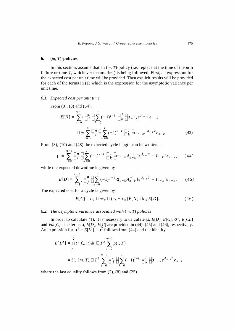
6. (m, T)-policies

In this section, assume that an (m, T)-policy (i.e. replace at the time of the m thfailure or time T, whichever occurs first) is being followed. First, an expression forthe expected cost per unit time will be provided. Then explicit results will be providedfor each of the terms in (1) which is the expression for the asymptotic variance perunit time.

6.1. Expected cost per unit time

From (3), (8) and (54),

E[ N ] = i ni

(− 1) i − k i

k

α n − k e An − k T e n − k

k = 0

i

∑i = 0

m − 1

∑

+ m ni

(− 1) i − k i

k

α n − k e An − k T en − k .

k = 0

i

∑i = m

n

∑

µ = ni

(−1) i − k i

k

α n − k An − k

− 1 [e An − k T − I n− k ]en − k ,k = 0

i

∑i = 0

m −1

∑ ( 4 4 )

From (8), (10) and (48) the expected cycle length can be written as

(43)

while the expected downtime is given by

E[ D] = j nj

(−1) j − k αn − k An − k

−1 [e An −k T − I n− k ]en − k .k = 0

j

∑j =1

m −1

∑ (45)

The expected cost for a cycle is given by

E[ C] = c0 + nc s + (c r − c s ) E[N ] + cd E[D]. (46)

E[ L2 ] =0

T

⌠ ⌡ t 2 fm ( t)dt + T 2 p(i, T )

i = 0

m −1

∑

= U2 ( m , T) + T 2 ni

( − 1)i − k i

k

αn − k eA n − k T en− k ,

k = 0

i

∑i = 0

m − 1

∑

6.2. The asymptotic variance associated with (m, T) policies

In order to calculate (1), it is necessary to calculate µ, E[D], E[C], σ 2, E[CL]and Var[C]. The terms µ, E[D], E[C] are provided in (44), (45) and (46), respectively.An expression for σ 2 = E[L2] – µ2 follows from (44) and the identity

where the last equality follows from (2), (8) and (25).


E[ CL] = ( c r − c s )x f1 ( x)d x

0

T

⌠ ⌡

=0

T

⌠ ⌡ ( cr − c s )x n

1

f (x ) [ 1− F (x)]n −1

= ( cr − c s ) n1

S3 ( n − 1, T ),

For m = 1, E[D] = E[D2] = 0,

and Var[C] = (cr – cs)2 {E[N 2] – E[N]2}.

In what follows, the more difficult case where m ≥ 2 is considered. From (52) inthe appendix: Use (2), 3) and (13), apply (18), (19) and (20) in (52) to get

Calculation of Var[C] is somewhat more complicated than the other calculations.First note that

Expressions for E[N] and E[D] are provided by (43) and (45), respectively. Conditionon the number of failures at time T and use (8) to obtain

E[ CL] = m 2 (c r − c s ) nm

( − 1)m −1− k m − 1

k

S3 (n − 1 − k , T ) (α A −1e)

k = 0

m −1

∑

+ c d m(m − 1) nm

(− 1)m − 2− k m − 2

k

{S1 (n − 2 − k , T )

k = 0

m − 2

∑

− S2 (n − 2 − k , T ) + (α A −1e)S3 (n − 2 − k , T ) }

+ T (c r − cs ) i ni

(− 1) i i

k

α n − k e An −k T en − k

k = 0

i

∑i = 1

m − 1

∑

+ Tcd i ni

(− 1) i − k −1 i

k

α n − k e An −k T en − k

k = 0

i

∑i = 1

m − 1

∑

{T − α A −1e AT e + α A − 1e} + µ (c0 + nc s ).

Var[ C] = (c r − c s ) 2 {E[ N 2 ] − E[N ] 2 } + 2 cd (c r − c s ) {E [ DN ] − E [D]E[ N ]}

+ cd2 {E [ D2 ] − E[ D] 2}.


E[ N 2 ] = i 2 p( i , T) + m 2 p(i , T )i = m

n

∑i = 0

m −1

∑

= i 2 ni

ik

(− 1) i − k α n− k e An− k T en− k

k = 0

i

∑i = 0

m −1

∑

+ m2 ni

ik

( − 1)i − k α n− k e An −k T en − k .

k = 0

i

∑i = 0

m −1

∑

E[ DN ] =0

T

⌠ ⌡ F (t )d t

i2 n

i

i − 1k

(− 1) i − k − 1[1 − F (T )]n − k − 1

k = 0

i − 1

∑i = 0

m −1

∑

+i = m

n

∑ m j ni

ij

k = 0

j

∑ (− 1) k + l jk

i − jl

l = 0

i − j

∑j = 1

m − 1

∑

⋅0

T

⌠ ⌡ [1 − F (t )]n − k − l

[1 − F (T )] l .

E[ DN ]

= {T − α −1e AT e + α A −1e} i 2 ni

(−1) i −1− k i −1

k

α n−k −1e An − k −1 T en− k −1

k =0

i−1

∑i =0

m −1

∑

Use expression (61) from the appendix to obtain

Apply (8), (10) and (13) to get

+i = m

n

∑ m j ni

ij

k = 0

j

∑ (− 1)k + l jk

i − jl

l = 0

i − j

∑j =1

m −1

∑ ⋅ α n − k − l [e An − k −l T − I n − k − l ]en− k − l (α l e Al T e l ).

E [ D2 ] = E[ I {τ m ≤ T} D 2 ] + E [ I{τ m > T } D2 ] . (47)

Thus, only the term E[D2] remains to be calculated. Note that

Thus, E[D2] can be computed by computing the two terms on the right-hand side of(47). Use (13) and (14) in (62) from the appendix to obtain

E[ I{τ m > T} D2 ]

= j nj

(− 1) j − 1− k j − 1

k

[α n− k −1e An − k −1 T en − k −1]

k = 0

j −1

∑j =1

m −1

∑


⋅ [ T 2 + 2T (α A −1e) + 2α( A −1) 2 e − 2α( A −1) 2 e AT e]

+ j( j − 1) nj

( − 1) j − 2− k j − 2

k

[α n − k − 2 e An − k− 2 T en− k − 2 ]

k = 0

j − 2

∑j = 1

m − 1

∑

⋅ [T − α A −1e AT e + α A −1e] 2 .

E[ I{τ m ≤ T} D2 ] = 2 U 3 (i , T ) − ( m − 1) 2 U1 ( m, T )i = 2

m − 1

∑

+ U4 (i , T ) + (m − 1) 2 U2 ( m , T ).i =1

m −1

∑

From (67) in the appendix: apply (29), (30), (31) and (32) to get

The above expressions are algebraically complex. However, for a given phase distri-bution, all reduce to tractable closed form expressions.

Example (continued). For n = 3, λ = 1.5 and co = 70, cs = 10, cr = 50, cd = 30, figures2 and 3, respectively, contain the expected costs and variance per unit time for (1, T),(2, T) and (3, T) failure policies as a function of T. The (2, 2.5) policy has the smallestexpected cost per unit time (79.97) and its associated variance is 1479.

7. Conclusion

Group maintenance policies form an important part of the reliability literature.However, the analyst has often been restricted to a very narrow (and often inappro-priate) range of distributions. Also, given the computational complexity of the prob-lems, sensitivity analyses where failure time and cost parameters can be varied havebeen problematic. By allowing the analyst to choose an arbitrary phase distribution,the applicability of group maintenance approaches is greatly increased. A contributionof this paper has been to provide explicit closed form results for the major policyclasses when the failure time has a phase distribution. These results, which in generalappear quite algebraically daunting, are computationally relatively easy for any givenproblem. This demonstrates once again that, as predicted by Neuts [9], use of phasedistributions can be of great practical utility. Sensitivity analyses are now very easy toconduct. Unlike most of the literature, the variability associated with group main-tenance policies has been explicitly modeled. (The results provided for calculatingthe asymptotic variability per unit time apply to general failure time distributions aslong as the first two moments are finite.) The closed-form results for the asymptoticvariance allow the analyst to consider criteria other than simply that of minimizingexpected cost per unit time. Indeed, in many applied situations, an analyst mightbe willing to tolerate an increased expected cost in order to reduce variability. In


Figure 2. Expected cost per unit time for (1, T), (2, T) and (3, T) failure policies;n = 3, co = 70, cs = 10, cr = 50, cd = 30.

Figure 3. Asymptotic variance per unit time for (1, T), (2, T) and (3, T) failure policies;n = 3, co = 70, cs = 10, cr = 50, cd = 30.


any case, even if choosing the policy that minimizes expected cost is the analyst’sobjective, knowledge of the associated variability provides important managerial infor-mation.

Appendix

This appendix is divided into two parts. In section A.1, expressions for calcu-lating (1) are derived. Section A.2 contains the phase results listed in section 3.

A.1. Calculating asymptotic cost and variance per unit time

Explicit expressions for the terms in (1) required to compute the asymptoticexpected cost and variance per unit time associated with (m, T) policies will now bederived. (Similar expressions for m-policies can be obtained by letting T → ∞ in theappropriate places.) The results of this section are general and apply to any continuousfailure distribution with finite first and second moments. (A summary of these resultstogether with some examples can be found in Wilson [16].)

A.1.1. Calculating µ, σ 2, E[CL] and E[C] for (m, T) policiesExpressions for µ, σ2, E[CL] and E[C] are provided by (48), (49), (52), and (55),

respectively.Expressions for µ and σ 2 follow by noting that

σ 2 = E [{min(T , tm )}2 ] − µ 2

=0

T

⌠ ⌡ t 2 fm ( t )dt + T 2 P (i , T ) −

0

T

⌠ ⌡ p( i, t )d t

i = 0

m − 1

∑

2

.i = 0

m −1

∑

y − E[ XjX < y] = y −

0

y

⌠ ⌡ P[X > t jX < y]dt = [ F (y)]− 1

0

y

⌠ ⌡ F (t )d t.

µ =0

T

⌠ ⌡ P[min(T ,τ m ) > t ]d t =

0

T

⌠ ⌡ p( i , t)dt

i = 0

m −1

∑ (48)

and

In order to calculate E[CL], it is first necessary to find expressions for E[CjL = T]and E[CjL = x], where x < T. Suppose that replacement occurs at x < T, i.e. replace-ment occurs at the m th failure. The downtime incurred over the cycle is the sum of thedowntimes for each of the first m – 1 failures. For any y > 0, the expected downtimefor an individual machine given that it has failed before time y and is replaced at timey is given by

(49)

Thus, for x < T,


E [Cj L = x] = c0 + mc r + (n − m) c s + cd (m − 1 ) [F (x)] −1

0

x

⌠ ⌡ F ( t)dt , (50)

E[ Cj L = T ] = c0 + ncs 0( c r − c s )E [ N f (T )jτ m ≥ T ]

+ cd P[N f (T ) = ijτ m ≥ T] i [F( T )]− 1

0

T

⌠ ⌡ F (t )d t,

i = 1

m − 1

∑

where the first three terms on the right-hand side represent the fixed and unit costs ofreplacing the system with a new one, while the last term is the expected downtimecost. Now suppose that the conditioning information is that the cycle ends at time T.Let Nf (t) denote the number of machines that have failed by time T. Then

where the first three terms represent the fixed and unit costs of replacing the systemwith a new one, while the last term is the expected downtime cost. Use (50) and (51)and the expression for µ given by (48) to obtain the following:

Let N and D, respectively, denote the random variables corresponding to the num-ber of failures and the downtime accumulated during a cycle. On noting thatE[min(T, τj)] = s0

T P[τ j > t]dt = s0T { p( i , t )}dti = 0

m − 1∑ , it can be seen that the expecteddowntime in a cycle is given by the following:

(51)

E[ D] = jE [min( T , τ j +1 ) − min(T ,τ j )]j =1

m −1

∑

=0

T

⌠ ⌡ j p( j , t)dt .

j = 1

m −1

∑

(52)

(53)

+ T i(cr − c s) + icd [ F (x )] −1 (T )

0

T

⌠ ⌡ F ( t)dt

p( i , T)

i =1

m −1

∑

+ ( co + ncs )

0

T

⌠ ⌡ p (i , t)dt .

i = 0

m −1

∑

E[ CL] = ⌠ ⌡ x E[C jL = x ]d G( x)

=0

T

⌠ ⌡ x E[C jL = x ] fm ( x)d x + T E[Cj L = T ]P[τ m ≥ T ]

=0

T

⌠ ⌡ m(c r − c s ) + cd (m − 1 ) [F ( x)] −1

0

x

⌠ ⌡ F ( t)dt

x f m (x )d x


E [ N ] = i p(i , T ) + m p( i, T ).j = m

n

∑j =1

m −1

∑ ( 5 4 )

E[ C] = co + nc s + (c r − c s) E[ N ] + cd E[ D]

= c o + c s + ( c r − c s ) i p( i ,T ) + m( vr − c s) p( i, T )j = m

n

∑j =1

m − 1

∑

+ cd

0

T

⌠ ⌡ j p( j , t )d t.

j = 1

m − 1

∑

Var[ C] = Var[ co − ncs + (c r − cs ) N + c d D]

= (c r − c s )2 {E [N 2 ] − E[ N ]2 }

+ 2c d (c r − c s ) {E [ DN ] − E [D] E[ N ]}

+ cd2 {E[ I{τ m ≤ T}D 2 ] + E [ I{τ m > T }D2 ]} − cd

2 {E [ D]2}.

Condition on the number of failures at time t to obtain the expected number offailures in a cycle:

Using (53) and (54), the expected cost incurred during a cycle can be written asfollows:

A.1.2. Calculating Var[C] for (m, T) policiesNow an expression for Var[C] will be provided. The variance of the cost of one

cycle is given by

(55)

(56)

Expressions for E[D] and E[N] are provided by (53) and (54), respectively.Expressions for E[N 2], E[DN], E[I{τm≤ T}D2] and E[I{τm >T}D2] will now be provided.These together with (53) and (54) can then be inserted into (56) for explicit evaluationof Var[C].

Condition on the number of failures at time T to obtain

E[ N 2 ] = i 2 p( i , T ) + m 2 p(i , T ).i = m

n

∑i = 0

m −1

∑ ( 5 7 )

E[ DN] = iE [DjN f (T ) = ij p(i , T ) + m E[DjN f (T ) = ij p(i , T ).

i = m

n

∑i = 0

m − 1

∑ ( 5 8 )

The random variable Nf (T) equals the actual number of failures if the system isreplaced at time T. If the system is replaced before time T, Nf , (T) represents the numberof failures that would have occurred up to time T if the system had not been replaced.Condition on the value of this random variable to obtain

From (52), for i < m,


E[ DjN f (T ) = i] = i[ F( T )]−1

0

T

⌠ ⌡ F (t )d t. ( 5 9 )

E[ DjN f (T ) = i] = jE [min( T, τ j +1 ) − minj =1

m −1

∑ (T ,τ j )jN f (T ) = i]

=0

T

⌠ ⌡ j P[N f ( t) = j jN f (T ) = i]d t

j = 1

m − 1

∑

=0

T

⌠ ⌡ j i

j

[ F (T )]− i [ F ( t)] j [F ( T ) − F( t)] i − j d t.

j = 1

m − 1

∑

Now consider the case where i ≥ m. Conditioned on Nf (T) = i, where i ≥ m, one has asystem of i independent machines. The (conditional) distribution function of the failuretime of one of these i machines equals [F(T)] –1F(·) since the only information aboutthe machine is that it would have failed before time T. So, in order to compute theexpected downtime conditioned on Nf (T) = i, one can act as if the system consists ofi (instead of n) machines with i.i.d. failure times with distribution function equal to[F(T)] –1F(·). Thus, for this system, the probability of j failures by time t is given by( j

i )[F (T ) −1 F (t )] j [1 − F (T ) − 1 F( t)] i − j .Use this and proceed as in (53) to obtain

Use (59) and (60) in (58) to obtain

E[ DN ] = [F (T )]−1

0

T

⌠ ⌡ F( t) dt i2 p(i ,T )

i =0

m −1

∑

+ m ni

i= m

n

∑0

T

⌠ ⌡ i

j

[1 − F (t )]n− i [F( t)] j [ F(T ) − F (t )] i− j dt

j =1

m −1

∑

.

(60)

(61)

It only remains to find expressions for E[I{τm >T}D2] and E[I{τm ≤ T}D2]. Suppose it isknown that exactly j < m machines have failed by time T. Then, conditioned on thisinformation, D has the same distribution as {∑ j

i =1(T – Yi)}, where Y1,…, Yj are i.i.d.random variables with density equal to [F(T)] –1f (·), the density of the time to failure,Y, of a single machine given that it fails by time T. Use this to obtain

E[ I{τ m > T} D2 ] = E [ D2jN f (T) = j] p( j ,T )

j = 1

m − 1

∑


where the last equality follows since the i.i.d. nature of the Yi implies thatE[(T – Yi)

2] = E[(T – Y)2] and E[(T – Yi)(T – Yj)] = E{[T – Y]}2, for i ≠ j. Use the re-sults that E[(T – Y)2] = s0

T(T – y)2F(T)–1f ( y)dy and E[T – Y] = s0T F(T)–1F( y)dy and

simplify to obtain

= E ( T − Yi )i = 1

j

∑

2

p( j ,T )j =1

m − 1

∑

+ { jE [( T − Y ) 2 ] + j( j − 1 ) (E [T − Y ]) 2 }p( j ,T ),j = 1

m −1

∑

E[ I{τ m > T} D2 ] = F ( T ) −1

0

T

⌠ ⌡ ( T − y ) 2 f (y) d y

j p( j ,T )

j =1

m − 1

∑

+ F ( T ) −1

0

T

⌠ ⌡ F ( t)dt

2

j ( j − 1) p( j , T )j = 1

m −1

∑

.

E[ I{τ m ≤ T} D2 ] = E I {τ m ≤ T} (τ m − τ i )i =1

m −1

∑

2

Suppose the m th failure occurs before time T ; then D = (τ m − τ i )i =1m − 1∑ . Use

this to obtain

E [ I{τ m ≤ T }τ i2 ] =

0

T

⌠ ⌡ x2 E [ I{τ m ≤ T }jτ i = x] f i ( x)d x

=0

T

⌠ ⌡ x2 P[ N f (T ) ≥ mjN f (x) = i] f i (x)d x.

For 2 ≤ i ≤ m,

Conditioned on the event {Nf (x) = i}, there are n – i functioning machines at time x,each of whose lifetime distribution function equals [1 – F(x)] –1F(·). For the event{Nf (T) ≥ m} to occur, at least m – i of these must fail by time T, i.e.

(62)

= E I{τ n ≤ T }

( m − 1) 2 τ m2 + τ i

2 − 2 (m − 1)τ m (τ m −1 + L + τ1)i = 1

m − 1

∑

+ 2 τ i (τ i −1 + L + τ1)i = 2

m −1

∑

. (63)


E [ I{τ m ≤ T }τ i2 ] =

0

T

⌠ ⌡ x2 K i ( x) f i (x) d x, ( 6 5 )

E[ I{τ m ≤T }τ i (τ i−1 + L+ τ 1 )] =0

T

⌠ ⌡ x Ki (x)E [τ i−1 + L+ τ 1jτ1 = x] f i (x) d x

=0

T

⌠ ⌡ x Ki (x) (i − 1)

0

x

⌠ ⌡ y[ F (x )] −1 f ( y)d y

f i ( x )d x.

P[ N f (T ) ≥ mjN f (x ) = i]

=j = m − i

n − i

∑ n − ij

{P[X ≤ T jX > x ]} j {P[ X > T jX > x]}n − i − j

= [1 − F (x )]− ( n− i )

j = m − i

n − i

∑ n − ij

[ F (T ) − F( x)] j [1 − F (T )]n − i − j .

Let Ki(x) denote (64), the probability that at least m machines will have failed bytime T given that exactly i have failed by time x. Thus,

for 2 ≤ i ≤ m. Note that conditioned on the events τi = x and {τm ≤ T}, the quantityτi –1 + … + τ1 is the sum of i – 1 independent failure times, each with density functionequal to F(x)–1f (·). Consequently,

Use (65) and (66) in (63) to obtain

E[ I{τ m ≤ T} D2 ] =0

T

⌠ ⌡ x2 f i (x)K i (x ) + (m − 1)2 fm ( x)

i =1

m −1

∑

d x

+ 2

0

T

⌠ ⌡ x ( i − 1) f i ( x)K i ( x) − ( m − 1) 2 fm (x)

i = 2

m − 1

∑

[ F( x)]−1

0

x

⌠ ⌡ y f ( y)d y

d x.

A.2. Derivation of expressions given in section 3

The following properties of the Kronecker product will be useful in the sequel.Let P, Q, U, V, W, Z be rectangular matrices such that the ordinary matrix productPQU and VWZ are defined; then

(64)

(66)

(67)


0

x

⌠ ⌡ αe At e d t = α A −1 ( e Ax − I )e

S1 ( j , T ) =0

T

⌠ ⌡ x 2 (α j e A j x ej ) (αe Ax A 0 )d x

=0

T

⌠ ⌡ x 2 (α j e A j x ej ) ⊗ (αe Ax A 0 )d x

=0

T

⌠ ⌡ x 2 (α j ⊗ α ) (e A j x ⊗ e Ax ) (e j ⊗ A 0 ) d x,

( PQU ) ⊗ (V W Z) = ( P ⊗ V ) (Q ⊗ W ) (U ⊗ Z). (68)

e ( P ⊗ I Q ) x + ( I P ⊗Q ) x = e Px ⊗ eQx , (69)

1 − [1 − F( t)] k = 1 − α k e Ak t e k , for k ≥ 2 (70)

0

x

⌠ ⌡ tα A − 1e At e dt = xα ( A − 1 ) 2 e Ax e − α( A −1 )3 ( eAx − I )e,

0

x

⌠ ⌡ α A −1e Ate dt = α ( A − 1 ) 2 (eAx − I ) e,

For any square matrices P and Q,

where IQ and IP are identity matrices of the same dimension as Q and P, respectively(see Neuts [10, p. 373]).

A.2.1. Derivation of (10)–(14)The function 1 – [1 – F(t)]k is the distribution function of min(X1,…, Xk) which

is a phase distribution with representation (αk, Ak). Consequently,

and s0T[1 – F(t)]kdt = s0

Tαke Aktek dt, from which (10) and (11) follow.Note that, for x > 0,

simplify and use integration by parts to obtain (12), (13) and (14).

A.2.2. Derivation of (18)–(20)Use (6) and (5) and apply (68) and (69) to obtain


S1 ( j , T ) =0

T

⌠ ⌡ x 2α j +1e A j+ 1 x d x

( e j ⊗ A 0 ),

where the second equality follows since the product of scalars is, trivially, a Kroneckerproduct. Now apply (68), (69) and the definition of αj +1 and A j+1 to obtain

from which (18) follows on integrating by parts twice.Use (6), (5) and apply (68) and (69) to obtain

S2 ( j , T ) =0

T

⌠ ⌡ x( αe Ax A 0 ) (α A − 1e Ax e) (α j e A j x e j )d x

=0

T

⌠ ⌡ x( αe Ax A 0 ) [ (α A −1 ⊗ α j )e A j +1 x e j + 1 ]d x,

where the last equality follows by applying (68) and using the definition of α j+1 andAj+1. Again, apply (68) and the definition of Aj +1 and ej+1 to obtain

S2 ( j , T ) =0

T

⌠ ⌡ x (α A −1 ⊗ α j e A j+ 1 x e j +1) ⊗ (αe Ax A 0 )d x

=0

T

⌠ ⌡ (α A −1 ⊗ α j ⊗ α) (eA j +1 x ⊗ e Ax )d x(e j +1 ⊗ A 0 )

=0

T

⌠ ⌡ [α A −1 ⊗ α j +1]e A j + 2 x d x(e j +1 ⊗ A 0 )),

from which (19) follows on applying integration by parts.Again, use (6), (5), (68) and (69) to obtain

S3 ( j , T ) =0

T

⌠ ⌡ x(α j e A j x e j ) (αe Ax A 0 )d x

=0

T

⌠ ⌡ xα j + 1e A j+ 1 x d x

(e j ⊗ A 0 ).

Integration by parts of the above expression yields (20).


A.2.3. Derivation of (29)–(32)Use the binomial theorem to expand [F(x)] i –1 = {1 – [1 – F(x)]} i–1 and [F(T) –

F(x)] i = {[1 – F(x)] – [1 – F(T)]}i in (2) and (28), respectively. Insert the resultingexpressions for f i(x) and Ki (x) into the definition for U3(i, T) and U4(i, T), gather termsand recall the definition of S1( · , · ), S2( · , · ) and S3( · , · ) to obtain the results givenin (31) and (32).

Similarly, (29) and (30) follow by inserting f i(x) into (24) and (25), expanding[F(x)] i –1 using the binomial theorem and recalling the definition of S1( · , · ), S2( · , · )and S3( · , · ).

References

[1] D. Assaf and J.G. Shanthikumar, Optimal group maintenance policies with continuous and periodicinspection, Management Science 33(1987)1440–1452.

[2] A. Bobbio and A. Cumani, Modeling wear-out by multistate homogeneous Markov models, in:Reliability in Electrical and Electronic Components and Systems, eds. C. Lauger and J. Moltorf,North-Holand, 1982, pp. 101–106.

[3] S. Chakravarthy, Analysis of production line systems with two unreliable machines with phase typeprocessing times and a finite storage buffer, Communications in Statistics: Stochastic Models 3(1987)369–391.

[4] M. Gururajan and K.S. Bhat, A complex priority redundant system with phase type distribution,Microelectronics and Reliability 30(1990) 453–455.

[5] M.A. Johnson, Selecting parameters of phase distributions: Combining nonlinear programming,heuristics, and Erlang Distributions, ORSA Journal of Computing 5(1993)69–80.

[6] M. Malhotra and A. Reibman, Selecting and implementing phase approximations for semi-Markovmodels, Communications in Statistics: Stochastic Models 9(1993)473–506.

[7] T.A. Mazzuchi and R. Soyer, A Bayesian perspective on some replacement strategies, ReliabilityEngineering and System Safety 61(1996)295–303.

[8] T. Nakagawa, Further results on replacement problem of a parallel system in a random environment,Journal of Applied Probability 16(1979)923–926.

[9] M. Neuts, Matrix-Geometric Solutions in Stochastic Models: An Algorithmic Approach, Johns HopkinsUniversity Press, Baltimore, 1981.

[10] M. Neuts, Algorithmic Probability: A Collection of Problems, Chapman and Hall, 1995.[11] K. Okumoto and E.A. Elsayed, An optimum group maintenance policy, Naval Research Logistics

Quarterly 30(1983)667–674.[12] E. Popova and J.G. Wilson, Selecting and implementing the best group replacement policy for a

non-Markovian system, in: Proceedings of the International Conference on Probabilistic SafetyAssessment and Management, eds. C. Cacciabue et al., Springer, 1996, pp. 58–63.

[13] P. Ritchken and J.G. Wilson, (m, T) group maintenance policies, Management Science 36(1990)632–639.

[14] S. Ross, Stochastic Processes, Wiley, New York, 1996.[15] W. Smith, Renewal theory and its ramifications, Journal of the Royal Statistical Society B 20(1958)

243–302.[16] J.G. Wilson, A note on variance reducing group maintenance policies, Management Science 42

(1996)452–460.[17] J.G. Wilson and A. Benmerzouga, Optimal m-failure policies with random repair time, Operations

Research Letters 9(1990)203–209.


[18] J.G. Wilson and A. Benmerzouga, Bayesian group replacement policies, Operations Research 43(1995)471–476.

[19] J.G. Wilson and E. Popova, Adaptive replacement policies for a system of parallel machines, in:Lifetime Data: Models in Reliability and Survival Analysis, eds. N.P. Jewell et al., Kluwer Academic,1996, pp. 371–375.

[20] J.G. Wilson and E. Popova, Optimal Bayesian group maintenance policies, Working Paper, Depart-ment of Mechanical Engineering, The University of Texas at Austin, Austin, 1997.


Documents

Group replacement policies for parallel systems whose ...popova/phase.pdfIn this paper, a system of stochastically independent and identical components is analyzed. Group replacement