Embed Size (px)
Citation preview

Group actions and ergodic theory on Banach function spaces
RJ de Beer
23914610
Thesis submitted for the degree Philosophiae Doctor in Mathematics at the Potchefstroom Campus of the North-West
University
Promoter: Prof LE Labuschagne
May 2014
i
Acknowledgments
There are several people without whom this work would never have been done.
I would like to thank my wife Bronwyn for her love and support along this some-
times steep and winding road.
I thank my mother, sister and friends for always believing in me.
The erudition and mathematical skill of my promoter, Prof. Louis Labuschagne
have been instrumental in guiding me through the subtleties of convex vector spaces
and function spaces. Far beyond that, his wisdom and good sense have made my
PhD studies fruitful.
This thesis belongs to all of you too.

ii
Group actions and ergodic theoryon Banach function spaces
Summary
This thesis is an account of our study of two branches of dynamical systems
theory, namely the mean and pointwise ergodic theory.
In our work on mean ergodic theorems, we investigate the spectral theory of
integrable actions of a locally compact abelian group on a locally convex vector
space. We start with an analysis of various spectral subspaces induced by the action
of the group. This is applied to analyse the spectral theory of operators on the
space generated by measures on the group. We apply these results to derive general
Tauberian theorems that apply to arbitrary locally compact abelian groups acting on
a large class of locally convex vector spaces which includes Frechet spaces. We show
how these theorems simplify the derivation of Mean Ergodic theorems.
Next we turn to the topic of pointwise ergodic theorems. We analyse the Trans-
fer Principle, which is used to generate weak type maximal inequalities for ergodic
operators, and extend it to the general case of σ-compact locally compact Haus-
dorff groups acting measure-preservingly on σ-finite measure spaces. We show how
the techniques developed here generate various weak type maximal inequalities on
different Banach function spaces, and how the properties of these function spaces in-
fluence the weak type inequalities that can be obtained. Finally, we demonstrate how
the techniques developed imply almost sure pointwise convergence of a wide class of
ergodic averages.
Our investigations of these two parts of ergodic theory are unified by the tech-
niques used - locally convex vector spaces, harmonic analysis, measure theory - and
by the strong interaction of the final results, which are obtained in greater generality
than hitherto achieved.
Keywords
Tauberian theorems, harmonic analysis, group action, spectral theory, mean er-
godic theory, Transfer Principle, maximal inequalities, Banach function spaces, point-
wise ergodic theory

iii
Groep aksies en ergodiese teorie op Banachfunksieruimtes
Samevatting
Hierdie tesis is ’n verslag van ons bestudering van twee takke van dinamiese
stelselteorie, naamlik die middel en puntsgewyse teorie.
In ons werk in middel ergoiese teorie, ondersoek ons die spektraalteorie van inte-
greerbare aksies van ’n lokaal kompakte abelse groep op ’n lokaal konvekse ruimte.
Ons begin met ’n analise van verskeie spektrale deelruimtes wat deur die groep-aksie
geınduseer word. Dit word toegepas om die spektraalteorie van operatore op die
ruimte voortgebring deur mate op die groep te analiseer. Ons pas hierdie resultate
toe om algemene Tauberse stellings af te lei wat toepasbaar is op arbitrere lokaal
kompakte abelse groepe wat op ’n groot klas van lokaal kompakte vektorruimtes in-
werk - ’n klas wat Frechet ruimtes insluit. Ons toon aan hoe hierdie stellings die
afleiding van middel ergodiese stellings vereenvoudig.
Daarna beskou ons die onderwerp van puntsgewyse ergodiese stellings. Ons
analiseer die Oordragsbeginsel, wat gebruik word om swak-tipe maksimale onge-
lykhede vir ergodiese operatore voort te bring, en brei die tegniek uit na die algemene
geval van σ-kompakte lokaal kompakte Hausdorff groepe wat maat-preserverend op
’n σ-eindige maatruimte inwerk. Ons toon aan hoe die tegnieke hier ontwikkel bring
voort verskeie swak-tipe maksimale ongelykhede op verskillende Banach funksieruimtes,
en hoe die eienskappe van hierdie funskieruimtes die swak-tipe ongelykhede wat ver-
werf word, beınvloed. Laastens, wys ons hoe die tegnieke wat ontwikkel is byna-oral
puntsgewyse konvergensie van ’n wye klas van ergodiese gemiddeldes impliseer.
Ons ondersoeking van hierdie twee dele van ergodiese teorie word geunieer deur die
tegnieke wat gebruik word - lokaal konvekse ruimtes, harmoniese analise, maatteorie
- en deur die sterk interaksie tussen die finale resultate, wat in groter algemeenheid
as vantevore behaal word.
Sleutelwoorde
Tauber stellings, harmoniese analise, groep aksie, spektraalteorie, middel er-
godiese teorie, Oordragsbeginsel, maksimale ongelykhede, Banach funksieruimtes,
puntsgewyse ergodiese teorie

Contents
Acknowledgments i
Summary and Keywords ii
Samevatting en Sleutelwoorde iii
1 The scheme of this work 1
1.1 Overview of ergodic theory . . . . . . . . . . . . . . . . . . . . . . . . 1
1.2 Mean ergodic theorems . . . . . . . . . . . . . . . . . . . . . . . . . . . 3
1.3 Pointwise ergodic theorems . . . . . . . . . . . . . . . . . . . . . . . . 4
1.4 Plan of the work on mean ergodic theorems . . . . . . . . . . . . . . . 6
1.5 Plan of the work on pointwise ergodic theorems . . . . . . . . . . . . . 8
2 Harmonic analysis & convex vector spaces 9
2.1 Locally convex vector spaces . . . . . . . . . . . . . . . . . . . . . . . . 10
2.2 Basics of vector-valued measure theory . . . . . . . . . . . . . . . . . . 13
2.3 Product spaces via vector-valued measure theory . . . . . . . . . . . . 16
2.4 Harmonic Analysis . . . . . . . . . . . . . . . . . . . . . . . . . . . . . 23
3 Banach function spaces 31
3.1 Basic definitions and constructions . . . . . . . . . . . . . . . . . . . . 31
3.2 Manipulations of fundamental functions . . . . . . . . . . . . . . . . . 37
3.3 Comparison of fundamental functions . . . . . . . . . . . . . . . . . . 39
3.4 Estimates of integrals and function norms . . . . . . . . . . . . . . . . 46
4 Mean ergodic theorems 56
4.1 Integrable Actions and Spectral Subspaces . . . . . . . . . . . . . . . . 56
iv

CONTENTS v
4.2 Operators on Spectral Subspaces . . . . . . . . . . . . . . . . . . . . . 67
4.3 Tauberian Theorems for Ergodic Theory . . . . . . . . . . . . . . . . . 70
4.4 Applications to Ergodic Theorems . . . . . . . . . . . . . . . . . . . . 74
4.5 Notes and Remarks . . . . . . . . . . . . . . . . . . . . . . . . . . . . . 77
5 Pointwise ergodic theorems 79
5.1 The Transfer Principle . . . . . . . . . . . . . . . . . . . . . . . . . . . 80
5.2 Semilocality and translation invariance . . . . . . . . . . . . . . . . . . 85
5.3 An example . . . . . . . . . . . . . . . . . . . . . . . . . . . . . . . . . 87
5.4 Kolmogorov’s inequality for r.i.BFSs . . . . . . . . . . . . . . . . . . . 88
5.5 The weak type of the transferred operator . . . . . . . . . . . . . . . . 91
5.6 Pointwise ergodic theorems . . . . . . . . . . . . . . . . . . . . . . . . 93
5.7 Notes and Remarks . . . . . . . . . . . . . . . . . . . . . . . . . . . . . 101
Bibliography 103
Index of Symbols 108

vi CONTENTS
Chapter 1
The scheme of this work
1.1 Overview of ergodic theory
Ergodic theory is a branch of dynamical systems theory where the long-term or
asymptotic behaviour of the system is studied. The abstract theory of dynamical
systems considered in this work is based on a distillation of experience in several fields
where concrete dynamical systems are essential. Physics of course provides a great
stimulus, as does number theory, where arguably ergodic theory has had even more
success. The dynamical systems viewpoint is also prominent in the representation
theory of topological groups [30] and even Ramsey theory [28]. One of the reasons
for these developments is the power of the abstract formulation of dynamics and the
ubiquity of questions of symmetry.
Perhaps surprisingly, it was in number theory, not physics, that ergodic ques-
tions concerning the asymptotic behaviour of systems first made an appearance.
As recounted in [36], Nicole Oresme (c. 1320-1382) had already anticipated Weyl’s
equidistribution result described below, and in his book Ad pauca respicientes used
it to prove that one cannot predict the position of planets long into the future, ren-
dering astrology devoid of meaning. In more modern times, one of the first profound
applications of the idea of examining the long term behaviour of a system was due
to Gauss, in his work on continued fractions. He found a limiting distribution (i.e. a
measure) that encodes the length of time the continued fraction algorithm will take
to approximate a given x ∈ (0, 1) by a rational number to a given degree of accuracy.
(See for example [2]).
1

2 CHAPTER 1. THE SCHEME OF THIS WORK
Of course the terms ergodicity and entropy were coined by the Austrian physicist
Karl Boltzmann in his work on statistical mechanics in the 1870s. The ergodic hy-
pothesis refers to the statement that if one takes the average of an observable over
time or over the phase space at a particular instant, one gets the same answer. Boltz-
mann’s goal was to develop statistical mechanics to the point where one could relate
macroscopic phenomena to the behaviour of the myriad elementary particles that
constitute the physical world. It is remarkable that he developed his theory in a time
where the atomic hypothesis of matter was in doubt.
In his work on celestial mechanics in the last decade of the 19th century, Henri
Poincare introduced new statistical techniques to the study of dynamical systems.
He proved that if the system is closed (we would now say that the phase space is
compact), then the system would return infinitely often and arbitrarily closely to
any previous configuration. This notion is even more starkly expressed measure
theoretically, in what is known as the Poincare Recurrence Theorem.
Returning to number theory, Hermann Weyl studied distribution problems in
number theory, greatly aiding the rise of statistical thinking in that deep and ancient
branch of mathematics. Bohl (1909), Weyl (1910) and Sierpinski (1910) proved that
if α is an irrational number, then the set nα mod 1 : n ∈ N is equidistributed
according to Lebesgue measure. Later in 1916, Weyl proved the same thing for n2α
mod 1, as did Vinogradov for the set pnα mod 1, where pn denotes the nth prime.
All these questions can be posed as an ergodic problem of certain dynamical systems.
Rosenblatt and Wierdl [40] is an excellent source for this material. At the forefront
of this line of thinking, we have for instance Bourgain [5] and [6], and Buczolich and
Mauldin [7]. These mathematicians consider far-reaching extensions of Birkhoff’s
original pointwise ergodic theorem. They show the pointwise convergence of averages
sampled on certain subsets of the natural numbers, such as the perfect squares. The
full ramifications of these results have yet to be fully explored.
In the 1930s, Erdos and Turan conjectured that any set of natural numbers with
positive upper Banach density must contain arbitrarily long arithmetic progressions.
This goes further than van der Waerden’s theorem of 1927, which states that if the
natural numbers are partitioned into a finite number of partitions, then at least one
of those partitions has arbitrarily long arithmetic progressions. The conjecture by
the two Hungarians was proved by another Hungarian, Szemeredi, in 1975. Hillel
Furstenberg [18] proved this result using ergodic theory, in particular multiple re-

1.2. MEAN ERGODIC THEOREMS 3
currence [18]. In conjunction with Katnelson and Ornstein, the proof was simplified
even further in [19]. The most spectacular success of this fusion of number theory
and ergodic theory in recent years has been Green and Tao’s proof that there are
arbitrarily long arithmetic progressions in the primes [23].
Broadly speaking, a measure-theoretic dynamical system consists of three ele-
ments: a Set X, a group G, and an action α, continuous in some sense, that binds
them together by mapping G into the group of automorphisms of X. In our work on
mean ergodic theorems, we take X to be a locally convex topological vector space, G
to be an abelian locally compact Hausdorff topological group and α to be a mapping
of G into the bicontinuous linear automorphism group Aut(X). This is made precise
in Definition 4.1.1. When dealing with pointwise ergodic theorems, X will be a σ-
finite measure space, G a locally compact Hausdorff group and α a mapping of G into
the group of measure preserving automorphisms of X. For the exact formulation, see
Definition 5.1.1.
The research contained in this thesis appears in two articles, [10] and [11]. The
first has already been published online on 25th February 2013, and the second has
been submitted and can be found at arxiv:1309.0125 [math.DS]. The material in
Sections 2.1, part of 2.2, 2.4 and Chapter 4 appears in [10]. The material in Sections
2.3, part of 2.2 and Chapters 3 and 5 appears in [11]. See Sections 4.5 and 5.7 for
further comments regarding the origin and attribution of the results.
1.2 Mean ergodic theorems
For the treatment of mean ergodic theorems, the aim of this thesis is to develop
enough spectral theory of integrable group actions on locally convex vector spaces
to prove Tauberian theorems, which are applicable to ergodic theory. A Tauberian
theorem is one where, given the convergence of a sequence or series in one sense, the
imposition of some condition on the sequence or series guarantees its convergence in
a stronger sense. The condition added is called a Tauberian condition. An excellent
overview of the subject, especially how it pertains to number theory, is given in
Korevaar [29]. It is noteworthy that Wiener proved a general Tauberian theorem
that has the Prime Number Theorem as a consequence. This proof, presented in
[43], is still one of the easiest proofs of that theorem.
The Tauberian theorems proved in Section 4.4 apply to the situation where a

4 CHAPTER 1. THE SCHEME OF THIS WORK
general locally compact abelian group acts on certain types of barrelled spaces, and
in particular all Frechet spaces. This generalises the Tauberian theorem shown in
[15], which applies only to the action of the integers on a Banach space. We use these
theorems to simply derive mean ergodic theorems in a rather general context.
The bulk of our development of the mean ergodic theory consists of using spectral
theory to transfer properties and constructions on a locally compact abelian group G
to the topological vector space X on which it acts. Put another way, we use spectral
theory to derive properties of a dynamical system from harmonic analytic properties
of the group.
Firstly, we outline the correspondence between certain subsets of the Pontryagin
dual G and certain closed G-invariant subspaces of X, called spectral subspaces. This
work was initiated by Beurling, closely followed by Godement in [21] and extended
by many authors; we refer especially to [1],[51],[35] and [47].
Secondly, the action of G on X naturally generates many continuous linear map-
pings from X to itself, by associating to every finite Radon measure µ on G a con-
tinuous endomorphism on X, called αµ. We discuss some characteristics of such
maps, particularly how they relate to the spectral subspaces. Also important here is
how properties of µ that can be determined by harmonic analysis are transferred to
properties of αµ.
The Tauberian theorems 4.3.1 and 4.3.2 are the focal point of our work on mean
ergodic theorems, extending results of Dunford and Schwartz [15] to a very gen-
eral setting. Mean ergodic theorems are proved for very general dynamical systems,
involving arbitray locally compact Hausdorff groups acting on Frechet spaces.
1.3 Pointwise ergodic theorems
Pointwise ergodic theorems have had an illustrious history spanning over 80 years
since G.D. Birkhoff first proved the foundational result in 1931. The proof of his
erogdic theorem has been so refined that one can give an elementary, leisurely demon-
stration in about two pages [26]. To work with more general ergodic averages however,
it seems one must still rely on a different approach. Indeed, one of the main tech-
niques that has been developed to prove pointwise ergodic theorems is supple enough
to deal with pointwise convergence phenomena for a great variety of different ergodic
averages, for different groups, function spaces and averages.

1.3. POINTWISE ERGODIC THEOREMS 5
This is the technique of maximal operators. The idea is that once one estimates
the behaviour of these maximal operators, proving the ergodic theorems becomes
quite simple. (We explain the proof strategy in Section 5.6 in the form of a three-
step programme). This is how the pointwise ergodic theorems are proved in [20] and
[40]. It is also how results on entropy and information are obtained in [36, Chapter
6].
In fact, Wiener [49] developed a method, later greatly embellished by Calderon
[8], for computing the requisite properties of the maximal operators, a method that
is the central theme of this work: the Transfer Principle. It is our goal to extend
the scope of this Principle and hence the scope of the maximal operator technique
in proving pointwise ergodic theorems. The Transfer Principle refers to a body of
techniques that allow one to transform certain types of operators acting on function
spaces over G to corresponding transferred operators acting on function spaces over
Ω, in such a way that many essential properties of the operator are preserved.
With regards to pointwise theorems and the technique of maximal operators, we
have four aims: firstly, to extend the Transfer Principle to a larger class of groups,
measure spaces and operators, secondly to broaden the reach of the techniques used
to determine the weak type of the transferred operator, thirdly to demonstrate how
properties of the function spaces on which the operators are defined influence the
weak type inequalities of the transferred operator, and finally to outline how these
results can be used to derive a number of new pointwise ergodic theorems.
We define the Transfer Principle in quite a general setting (Definition 5.1.2). If
the operator to be transferred - call it T - is linear, then G and Ω need only be σ-finite
(Definition 5.1.7) and if it is sublinear, then it must have separable and metrisable
range (Definiton 5.1.6). The determination of the weak type of the transferred oper-
ator - call it T#- rests on results requiring Ω to be countably generated and resonant
as defined just before Proposition 3.4.1. This fulfills the first aim.
Computing the weak type of the transferred operator T# is achieved with Corol-
lary 5.5.2, especially in combination with Lemma ??. A noteworthy feature of these
results is that they show how the most important factors determining the weak type
of T# are the fundamental functions associated with the function spaces defining the
weak type of T . In this way, the problem of computing the weak type of the trans-
ferred operator is reduced to computations involving certain well-behaved real-valued
functions. In particular, these results allow us to estimate the weak type of the max-

6 CHAPTER 1. THE SCHEME OF THIS WORK
imal operator associated with ergodic averages over a wide class of rearrangement
invariant Banach function spaces. This completes the second aim.
For the third aim, we use such properties as the Boyd and fundamental indices of
a rearrangement invariant Banach function space X and show how straightforward
weak type (p, p) inequalities of T can be transferred to weak type inequalites for T#
acting on X.
Finally, we address the fourth aim by proving pointwise ergodic theorems, trans-
ferring information obtained using Fourier analysis on the group to properties of the
ergodic averages, and information on the function space on which they act, that
is encoded in the fundamental function. The main results are Theorem 5.6.6 and
Corollaries 5.6.7 and 5.6.8.
The importance of the Transfer Principle in ergodic theory has long been ap-
preciated - see the excellent overview given in [3]. Apart from Calderon’s seminal
paper [8], this principle is treated in some detail in the monograph [9] and employed
extensively in [40]. In [34] the author makes use of Orlicz spaces to prove results
about the pointwise convergence of ergodic averages along certain subsets of the nat-
ural numbers. In [16] the Transfer Principle of Coifman and Weiss is extended to
Orlicz spaces with weight for group actions that are uniformly bounded in a sense
determined by the weighted Orlicz space.
1.4 Plan of the work on mean ergodic theorems
The plan of our work on mean ergodic theorems is as follows. Sections 2.4 and 2.1
contain some basic material on harmonic analysis and topological vector spaces. First,
there is a brief discussion on the harmonic analysis required and includes extensions
of known results, most notably Theorem 2.4.1. There follows some work on locally
convex topological vector spaces and vector-valued measures. These results form the
core of the techniques used to transfer information from the group to the topological
vector space upon which it acts.
In Section 4.1, we discuss integrable actions of G on E. We shall do so using gen-
eral topological considerations and employing a little measure theory of vector-valued
measures, in the hope that it will bring some clarity to the idea (Definition 4.1.1).
This definition elaborates on an idea introduced in [1] and is discussed elsewhere,

1.4. PLAN OF THE WORK ON MEAN ERGODIC THEOREMS 7
such as in [35], [47] and [51]. In this work, we stress the continuity properties that
a group action may have, and how such continuity properties can be analysed using
vector-valued measure theory. Next we introduce spectral subspaces by providing the
definitions that appear in [1], [35] and [21], namely Definitions 4.1.6 and 4.1.8. We
demonstrate that they are in fact the same. There is a third kind of spectral subspace
given in Definition 4.1.10. It is important because it is directly related to a given
finite Radon measure and provides a link to the associated operator. We show how
this type of spectral subspace is related to the first two mentioned. Finally we show
how to employ the tool of spectral synthesis in harmonic analysis to analyse spectral
subspaces. Here the highlight is Theorem 4.1.15.
We discuss properties of operators on E induced by finite Radon measures on
G in Section 4.2. A major theme is how properties of the Fourier transform of a
measure determine how the associated operator will act on spectral subspaces. This
underlines the intuition that the Fourier transform on the group side of an action
corresponds to spectral spaces on the vector space side. For the development of
the Tauberian theorems, we need to know how to transfer convergence properties of
sequences of measures to convergence properties of sequences of operators. This is
done in Proposition 4.2.3. We prove these results by applying our knowledge of the
relationship between a convergent sequence of measures and its sequence of Fourier
transforms as set out in Section 2.4, as well as the link between spectral synthesis
and spectral subspaces.
Having developed enough spectral theory, we come to the highlight of this work:
the Tauberian theorems 4.3.1 and 4.3.2. Apart from being generally applicable to
situations where a locally compact abelian group G acts on a Frechet space X, it
also handles general topologies of the action − where the action is continuous in the
weak or strong operator topologies as well as intermediate topologies. We also discuss
some general cases in Remark 4.3.3 where the hypotheses of the Tauberian theorems
are automatically satisfied.
In Section 4.4 we show how, from the Tauberian results, we can quickly deduce
mean ergodic theorems for general locally compact abelian groups acting on Frechet
spaces.

8 CHAPTER 1. THE SCHEME OF THIS WORK
1.5 Plan of the work on pointwise ergodic theorems
Let us briefly describe the organisation of the our work on pointwise ergodic theorems.
In Section 5.1, we define the Transfer Principle and analyse it in some detail. This
involves quite intricate measure-theoretic considerations, including the development
of a theory of locally Bochner integrable functions in parallel with the classical theory
of Bochner integrable functions.
In Section 3.1 we bring to mind some basic constructions and definitions in the
theory of rearrangement invariant Banach function spaces. We emphasise how in the
general theory a central role is played by the fundamental function of such spaces,
and how a great deal of their structure and behaviour is reflected in this function.
Propositions 3.4.2 and 3.4.3 extend work of O’Neil [33] on tensor and integral products
by showing how under certain conditions the hypotheses of Theorems 8.15 and 8.18
in [33] can be weakened. We also estimate other integrals that arise naturally for
functions on product spaces (Proposition 3.4.1).
Section 5.5 contains the main results for estimating the weak type of the trans-
ferred operator, namely Corollary 5.5.2, and is based on the work of the previous two
sections including an extension of an inequality of Kolmogorov (Theorem 5.4.1).
In the final part of the work, Section 5.6, we explain a general method for deriving
pointwise ergodic theorems from maximal inequalities. This reduces the tack of
proving almost everywhere convergence to checking certain group theoretic properties
of the desired average using harmonic analysis, in particular the Fourier transform.
We show again how properties of the averages, the space acted upon and the nature
of the action interact to yield the almost everywhere convergence of ergodic averages.

Chapter 2
Harmonic analysis and locally
convex vector spaces
The mean and pointwise ergodic theorems that are our ultimate goal depend on a
thorough understanding of two very subtle subjects, namely that of locally convex
topological vector spaces and harmonic analysis. Both have been central to the
development of 20th century mathematics and are associated with the great names in
analysis and number theory. We bring to mind some of the most important objects
and constructions in both.
For the material on locally convex spaces we draw principally from [38], but
also [24] and [45] for more advanced information. For harmonic analysis we follow
Folland [17], Rudin [41] and Katznelson [25]. Folland also deals with nonabelian
groups, taking the representation theoretic viewpoint, whereas Rudin covers abelian
group theory in detail, going more deeply into the structure theory of such groups.
Because we are dealing with topological group actions, quite a bit needs to be
said about the way measure spaces (such as the group) interact with vector spaces.
This leads us to vector-valued measure theory, which is masterfully treated by Diestel
and Uhl [14] and Ryan [44].
In Section 2.1 we discuss the algebraic concept of a dual pair of Banach spaces
and how one can use it to define three of the most important topologies on a vector
space: the weak, Mackey and strong topologies. These will play an essential role in
the mean ergodic theory.
In Section 2.2 we develop extensions of the standard vector-valued measure theory.
9

10 CHAPTER 2. HARMONIC ANALYSIS & CONVEX VECTOR SPACES
In the mean ergodic theory, this extension is crucial to understanding the different
ways in which a group can act on a vector space. Section 4.1 relies heavily upon it. In
the pointwise ergodic theory, it will be crucial to working with the transfer principle,
in particular proving properties of the transferred operator in Section 5.1.
In Section 2.3 we shall use this theory of vector-valued measures combined with
results on injective and projective tensor products of locally convex vector spaces
to work with product measure spaces. This will be needed in the pointwise theory
where we must frequently work with the Cartesian product of the group with another
measure space. The vector-valued measure approach allows us to effectively deal with
these questions.
Section 2.4 covers harmonic analysis, including extensions of known results and
applications of the convex space theory to spaces that naturally arise out of the
harmonic analysis itself.
We shall denote the Haar measure on the locally compact group G by the symbol
h.
One final notational convention: if A is a measurable subset of a measure space
(Ω, µ), for brevity we shall write |A| := µ(A). Likewise, if K is a measurable subset
of the locally compact group G, we shall denote by |K| the Haar measure of K.
2.1 Locally convex vector spaces
We now mention some aspects of the theory of locally convex topological vector
spaces. A pair of complex vector spaces (E,E′) is said to be a dual pair if E′ can be
viewed as a separating set of functionals on E and vice versa. For example, a Banach
space X and its dual X∗ are in duality.
The spaces E and E′ induce upon each other certain topologies via their duality.
We denote the smallest such topology, the weak topology, by σ(E,E′), and the largest,
the strong topology, by β(E,E′). The latter is generated by sets of the form A =
x ∈ E : |〈x, a〉| ≤ 1 for all a ∈ A, as A ranges over all σ(E′, E)-bounded subsets
of E′. The set A is called the polar of A. There is also the Mackey topology,
called τ(E,E′), which is the finest locally convex topology on E such that under this
topology, E′ is exactly the set all continuous linear functionals on E.
Suppose (E,E′) and (F, F ′) are dual pairs. The set of all σ(E,E′) − σ(F, F ′)-
continuous linear mappings between topological vector spaces E and F is denoted
2.1. LOCALLY CONVEX VECTOR SPACES 11
by Lω(E,F ). The set of all β(E,E′)− β(F, F ′)-continuous linear mappings between
topological vector spaces E and F is denoted by Lσ(E,F ).
Now any linear map T : E → F is σ(E,E′)−σ(F, F ′)-continuous if and only if it is
τ(E,E′)− τ(F, F ′)-continuous. Also, if T : E → F is σ(E,E′)−σ(F, F ′)-continuous,
then it is β(E,E′)− β(F, F ′)-continuous. Hence Lω(E,F ) ⊂ Lσ(E,F ).
A linear map from a Frechet space X to a locally convex topological vector space
is continuous if and only if it is bounded. Hence the set B(X) of all bounded linear
mappings from X to itself is precisely the set of all τ − τ and hence σ−σ-continuous
linear mappings. On a Frechet space, the τ and β topologies are the same, so in this
case we have Lω(X) = Lσ(X) = B(X). Because of this, we automatically view a
Frechet space as a pair in duality, given as (X,X∗).
A set A ⊂ E is said to be bounded if for every neighbourhood V ⊂ E of the
identity, there is a λ > 0 such that A ⊆ λV .
The weak operator topology (wot) and the strong operator topology (sot) can
be described in terms of dual pairs. The pair (Lω(E), E ⊗ E′) is in duality via the
bilinear form
〈T, x⊗ y〉 := y(T (x)).
(Here ⊗ denotes the algebraic tensor product between the two vector spaces.) Then
the wot on Lω(E) is generated by the polars of all finite subsets of E ⊗ E′. The
sot is generated by polars of the form A⊗B where A is a finite subset of E and B
a ξ-equicontinuous subset of E′. (This condition on B means that for every ε > 0,
there is a ξ-neighbourhood V of 0 in E such that b(V ) ⊆ [−ε, ε] for all b ∈ B.)
The theory of locally convex topological vector spaces is at the same time notori-
ously tricky and vastly general. Let us include two short results demonstrating some
of the techniques required to prove facts about different locally convex toplogies, and
how these topologies interact.
Lemma 2.1.1. Let (E,E′) and (F, F ′) be two pairs of vector spaces in duality. Sup-
pose that t : E → F and its transpose t′ : F ′ → E′ are both bijective linear maps.
Then t is a homeomorphism between E and F when both are given their weak topolo-
gies, their Mackey topologies or their strong topologies.
Proof. By [38, Ch. II, Prop 12, p38], both t and its inverse t−1 are continuous when
E and F have their weak topologies.

12 CHAPTER 2. HARMONIC ANALYSIS & CONVEX VECTOR SPACES
Hence by [38, Ch. III, Prop 14, p62], both t and its inverse are continuous when
E and F have their Mackey topologies.
Finally, suppose that both E and F have their strong topologies. We show that
t is β(E,E′) − β(F, F ′)-continuous. If U ⊂ F is a neighbourhood in F , then under
the β(F, F ′)-topology there is a B ⊂ F ′ such that B ⊆ U . Now as shown above,
t′ : F ′ → E′ is σ(F ′, F )− σ(E′, E)-continuous, so t′(B) is σ(E′, E)-bounded in E′.
By [38, Ch. II, Lemma 6, p39], (t−1(B)) = t′(B). By [38, Ch. II, Theorem 4,
p35] and [38, Ch. IV, Lemma 1, p44], B ⊆ F ′ is also bounded. Hence by the weak
continuity of t−1, so is (t−1(B)).
Therefore t−1(B) is a neighbourhood in the β(E,E′)-topology, proving the con-
tinuity of t−1. In exactly the same way we can prove the strong continuity of t.
Lemma 2.1.2. Let (E,E′) be a dual pair with E barreled and let (tγ)γ∈Γ be a net
of continuous functionals in the β(E,E′)-topology. Suppose that tγ → t pointwise on
E. Then t is also β(E,E′)-continuous.
Proof. This is essentially the Banach-Steinhaus theorem. By [38, Ch. IV, Theorem
3, p69], the set tγ is equicontinuous on E. This means that for any ε > 0, there is
a neighbourhood U ⊂ E such that |tγ(U)| ≤ ε for all γ ∈ Γ. Then if x ∈ U ,
t(x) = limγ→∞
tγ(x) ∈ [−ε, ε].
Thus t is continuous too.
Finally, we frame a well-known mode of convergence in terms of a particular
topology constructed by the techniques developed in [38]. In the sequel, we shall
require several such reformulations, so it might be of use to see the process in action
in a simple case. Recall that M(X) is the space of all Radon measures on X.
Lemma 2.1.3. If X is a locally compact Hausdorff space and (fn) ⊂ Cb(X) is a
bounded sequence of continuous functions converging uniformly on compact subsets
of X, then (fn) is convergent in the σ(Cb(X),M(X))-topology.
Proof. For any Y ⊂ X and g ∈ Cb(X), let ‖g‖Y = sup|g(y)| : y ∈ Y . Let A =
sup‖fn‖X. Obviously, (fn) converges to a continuous function f , and ‖f‖X ≤ A.
For any µ ∈M(X), we must show that∣∣∣∣ ∫Xfn dµ−
∫Xf dµ
∣∣∣∣→ 0

2.2. BASICS OF VECTOR-VALUED MEASURE THEORY 13
as n→∞.
Let ε > 0 be given. As µ is a finite Radon measure on X, there is a compact
subset K ⊂ X such that µ(X\K) < ε/4A. Furthermore, (fn) converges uniformly to
f on K, and so there is an N ∈ N such that for all n ≥ N , ‖fn − f‖K < ε/2µ(K).
Hence for all n ≥ N ,∣∣∣∣ ∫Xfn dµ−
∫Xf dµ
∣∣∣∣ ≤ ∫X|fn − f | dµ =
∫X\K
|fn − f | dµ+
∫K|fn − f | dµ
≤ ‖fn − f‖X\Kµ(X\K) + ‖fn − f‖Kµ(K)
< 2A.ε/4A+ (ε/2µ(K))µ(K)
= ε.
2.2 Basics of vector-valued measure theory
We make some remarks on measurable vector-valued functions on a measure space
(Ω, µ). We require an extension of the theories of Bochner and Pettis integrable func-
tions to functions taking values not in a Banach space, but more general locally convex
vector spaces. We will also need a theory of locally Bochner integrable functions. Let
(Ω, µ) be a σ-finite measure space and E a complete locally convex vector space whose
topology is defined by the family pαα∈Λ of seminorms. Here the theory and proofs
closely follow the standard treatments for Banach space-valued functions, such as [44]
or [14]. A µ-simple measurable function f : Ω → E is a function f =∑N
i=1 χEixi,
where E1, . . . , EN are µ-measurable subsets of Ω and x1, . . . , xN ∈ E. A function
f : Ω → E is said to be µ-measurable if there is a sequence of µ-simple measurable
functions (fn) that converges µ-almost everywhere to f .
A function f : Ω → E is said to be µ-weakly measurable if the scalar-valued
function e′f is µ-measurable for every e′ ∈ E′ and Borel measurable if for every
open subset O of E, f−1(O) is a measurable subset of Ω. Finally, f is µ-essentially
〈separably/ metrisably〉 valued if there is a µ-measurable subset A of Ω whose comple-
ment has measure 0, such that f(A) is contained in a 〈separable/metrisable〉 subspace
of E.
It is worth noting that there are locally convex separable vector spaces that are
not metrisable. The strict inductive limit topology discussed in [38, Section VII.1]

14 CHAPTER 2. HARMONIC ANALYSIS & CONVEX VECTOR SPACES
can be used to construct such topologies.
Theorem 2.2.1. (Pettis Measurability Theorem) For a σ-finite measure space
(Ω, µ) and dual pair (E,E′), the following are equivalent for a µ-essentially metrisably
valued function f : Ω→ E:
1. f is µ-measurable
2. f is µ-weakly measurable and essentially separably valued
3. f is Borel µ-measurable and essentially separably valued.
The proof of this theorem is a straightforward adaptation of the proof of the
Banach space-valued proof presented in [44]. In particular, if E is separable and
metrisable, the measurability and weak measurablility of a function are equivalent.
In the proof of this Theorem in [44], the following fact is quoted without proof. It
remains crucial when handling metrisably valued measurable functions, so we record
it here for completeness.
Lemma 2.2.2. In a separable metric space X, any open set U is the union of count-
ably many closed balls.
Proof. Let xi be a countable dense subset of U . For each xi, define
di = d(xi, Uc) = infd(xi, u
′) : u′ ∈ U c
ri = di(1− 1/2i)
Bi = x ∈ X : d(x, xi) ≤ ri.
Then the sets Bi are closed and Bi ⊂ Ui. The proof will be complete when we show
that U = ∪iBi.Take any u ∈ U . If u is an isolated point, then u ∈ xi and so u ∈ Bi for some i.
Otherwise, let d = d(u, U c) and S = i : d(u, xi) < d/2. By the triangle inequality,
for any u′ ∈ U c and i ∈ S, we have
d(u, u′) ≤ d(u, xi) + d(xi, u′).
Taking infimums over the u′ first on the left and then on the right of the inequality
and using the fact that i ∈ S, we get d < d/2 + di and so
d/2 < di.

2.2. BASICS OF VECTOR-VALUED MEASURE THEORY 15
As S is infinite, we can find an i such that d/2 < ri. Hence d(xi, u) < ri and
u ∈ Bi.
We define the integral of a simple measurable function s =∑N
i=1 χEixi over a set
A ⊂ Ω of finite measure by defining∫As dµ =
n∑i=1
µ(A ∩ Ei)xi.
Turning to the question of the integrability of vector-valued functions, we shall re-
quire two different integrals. We define the integral of a µ-simple measurable function
f =∑N
i=1 χEixi to be ∫Ωf dµ =
∫Ω
N∑i=1
xiχi dµ =N∑i=1
µ(Ei)xi (2.1)
Definition 2.2.3. Consider a σ-finite measure space (Ω, µ) and dual pair (E,E′)
under a topology ξ and let f : Ω→ E be a vector valued function.
1. If f is µ-weakly measurable, we say that it is µ-Pettis integrable if for every
µ-measurable subset A ⊂ Ω there is an element∫A f dµ ∈ E such that for all
e′ ∈ E′, ⟨ ∫Af dµ, e′
⟩=
∫A
⟨f(ω), e′〉 dµ(ω). (2.2)
2. If f is µ-measurable and Pettis integrable, we say that it is µ-Bochner inte-
grable if there exists a sequence (fn) of µ-simple measurable functions converg-
ing a.e. to f , such that for every equicontinuous subset A ⊂ E′∫Ω
supe′∈A|〈f(x)− fn(x), e′〉| d|µ|(x) −→ 0 (2.3)
as n→∞.
In the definition of the Bochner integral, the hypothesis that the function is Pettis
integrable ensures that the sequence (∫
Ω fndµ) is not only Cauchy, but convergent.
We define the Bochner integral of a µ-Bochner integrable function by the limit∫Ωf(x) dµ(x) = lim
n→∞
∫Ωfn(x) dµ(x).
The proof of the existence of this limit and its independence from the particular
sequence of µ-simple measurable functions chosen, works exactly as in the Banach-
valued case.

16 CHAPTER 2. HARMONIC ANALYSIS & CONVEX VECTOR SPACES
Lemma 2.2.4. If f is µ-Bochner integrable from the measure space (Ω, µ) into the
locally convex vector space E, then for any equicontinuous A ⊂ E′ we have
supe′∈A
∣∣⟨ ∫Ωf dµ, e′
⟩∣∣ ≤ ∫Ω
supe′∈A|〈f(x), e′〉| d|µ|(x). (2.4)
Equivalently, one can define local Bochner integrability in terms of the seminorms
definining the topology on E. In this language, f is locally Bochner integrable if there
exists a sequence of measurable simple functions (fn) converging almost everywhere
to f and satisfying
limn→∞
∫Apα(f − fn) = 0
for every finitely measurable subset A ⊂ Ω and every seminorm pα.
These integrability concepts will be crucial to understanding continuity properties
of the action of a group on a locally convex vector space and will be used in Definition
4.1.1.
2.3 Product spaces via vector-valued measure theory
On the space of measurable functions over a measure space (Ω, µ) we can define a
family of seminorms pA(f) :=∫A |f | dµ as A ranges over all subsets of Ω of finite
measure. Those measurable functions for which pA(f) is finite for all A of finite
measure form the locally convex vector space of locally integrable functions. This
space is called Lloc(Ω) and is topologised by the family pA.If we have two measure spaces (Ω1, µ1) and (Ω2, µ2) then we can consider the
family of seminorms pA×B defined on the set of measurable functions on (Ω1×Ω2, µ1×µ2) by setting pA×B(f) =
∫A×B |f | dµ1×µ2 and define Lr−loc(Ω1×Ω2), the space of
all rectangular locally integrable functions, to consist of those measurable functions
for which all such seminorms are finite. As with the locally integrable functions, we
use the family pA×B to define the topology on Lr−loc(Ω1 × Ω2).
In the category of locally convex spaces, it is possible to topologise the tensor
product of two spaces in many ways. Two such tensor topologies can be distinguished:
the projective tensor product used above and the injective tensor product. Here is
one of two results on projective tensor products that we shall need.
Proposition 2.3.1. If (Ω1,Σ1, µ1) and (Ω2,Σ2, µ2) are two σ-finite measure spaces,
then there is a continuous linear injection ι1 : Lr−loc(Ω1 × Ω2)→ Lloc(Ω1)⊗πLloc(Ω2).

2.3. PRODUCT SPACES VIA VECTOR-VALUED MEASURE THEORY 17
Proof. The space Lloc(Ω1) may be recognised as the projective limit of the family of
spaces L1(A), as A ranges over all finitely measurable subsets in Σ1 and mappings
rBA : L1(B) → L1(A) where B ⊇ A and rBA is the restriction map. Similarly for
Lloc(Ω2). Hence by [24, Theorem 15.2], Lloc(Ω1)⊗πLloc(Ω2) is the projective limit of
the family L1(A)⊗πL1(B), as A and B range over all finitely measurable subsets of
Ω1 and Ω2 respectively.
Now L1(A)⊗πL1(B) ' L1(A × B) as shown for example in [44]. As the re-
striction maps rA×B : Lr−loc(Ω1 × Ω2) → L1(A × B) are well-defined and con-
tinuous, from the universal property of the projective limit (as described in [31,
Chapter 3.4] or [48, Appendix L]) there is a unique continuous linear mapping
ι1 : Lr−loc(Ω1 × Ω2) → Lloc(Ω1)⊗πLloc(Ω2) such that the following diagrams com-
mute for all finitely measurable A ∈ Σ1 and B ∈ Σ2.
Lr−loc(Ω1 × Ω2)
L1(A×B)
Lloc(Ω1)⊗πLloc(Ω2)ι1
rA×BrA ⊗ rB
It is clear from this diagram that ι1 is injective: if f and g are distinct elements
of Lr−loc(Ω1 × Ω2), then there is some rectangle A×B on which they are not equal
a.e.; this means that rA×B(f − g) 6= 0 and so ι1(f − g) 6= 0.
We now note the result about the injective product that we shall employ, namely
that if X is locally compact Hausdorff and E is a complete locally convex vector
space then
C(X,E) ' C(X)⊗εE
where C(X,E) and C(X) denote respectively the continuous E-valued and C-valued
functions on X equipped with the compact-open topology and ⊗ε denotes the com-
pletion of the injective tensor product of the two spaces. This result is proved in [24,
Corollary 3, Section 16.6].
The locally convex space of all locally Bochner integrable E-valued functions is
called Lloc(Ω, E) and its topology is given by the family of seminorms πA,α defined
by πA,α(f) =∫A pα(f) dµ, where A is a subset of Ω of finite measure and pα is one
of the seminorms that defines the topology on E.

18 CHAPTER 2. HARMONIC ANALYSIS & CONVEX VECTOR SPACES
In the case where E is a Banach space, it is well-known that L1(Ω, E) ' L1(Ω)⊗πE,
which is proved in detail in [44] and [14]. From this fact, we can construct a similar,
though weaker, relation between Lloc(Ω, E) and Lloc(Ω)⊗πE where E is a complete
locally convex space, which is given in the following lemma.
Lemma 2.3.2. There is a naturally defined continuous injective mapping ι2 : Lloc(Ω, E)→Lloc(Ω)⊗πE.
Proof. We shall work once more with restriction maps as we did in Proposition
2.3.1. Any locally convex space E is the projective limit of a family of Banach spaces
Eα. For every α, let qα : E 7→ Eα be the continuous linear mapping induced by the
projective limit. Then we can define q′α : Lloc(Ω, E)→ Lloc(Ω, Eα) to be the mapping
f 7→ qα f .
For any subset A ⊆ Ω of finite measure, define rA : Lloc(Ω, E) → Lloc(A,E) to
be the restriction map f 7→ f∣∣A
.
Now we can define maps πA,α : Lloc(Ω, E) → L1(A,Eα) by setting πA,α := rA q′α = q′α rA. On the other hand, there are the mappings rA ⊗ qα : Lloc(Ω)⊗πE →L1(A)⊗πEα. Identifying L1(A)⊗πEα and L1(A,Eα), we see that Lloc(Ω)⊗πE is the
projective limit of the family L1(A,Eα). By the universal property of the projective
limit, there must be a unique mapping ι2 : Lloc(Ω, E) → Lloc(G)⊗πE such that the
diagrams
Lloc(Ω, E)
L1(A,Eα)
Lloc(Ω1)⊗πEι2
πA,αrA ⊗ qα
commute for all α and finitely measurable A. From these diagrams the injectivity of
ι2 is clear.
There is a strong link between the spaces Lr−loc(G × Ω), Lloc(Ω, Lloc(G)) and
Lloc(G)⊗πLloc(Ω) that builds on Proposition 2.3.1 and Lemma 2.3.2. (Here G is a
locally compact Hausdorff group acting on the measure space Ω.) To establish this
link, we need the following elementary lemma.
2.3. PRODUCT SPACES VIA VECTOR-VALUED MEASURE THEORY 19
Lemma 2.3.3. If (Ω1, µ1) and (Ω2, µ2) are σ-finite measure spaces then the collection
of rectangular simple functions with support of finite measure is dense in Lr−loc(Ω1×Ω2).
Proof. Let f ∈ Lr−loc(Ω1 × Ω2) be a [0,∞]-valued function. To prove the Lemma,
it suffices to show that there is an increasing sequence (fn) of non-negative rectan-
gular simple functions with support of finite measure such that limn→∞ fn(ω1, ω2) =
f(ω1, ω2) µ1 × µ2-a.e., because then by the Monotone Convergence Theorem
limn→∞
∫A×B
|f − fn| dµ1 × µ2 = 0
for any µ1 × µ2-finite rectangle A×B. By [42, Theorem 1.17] there is an increasing
sequence of simple functions (gn) converging pointwise a.e. to f . We may assume
that each gn has µ1 × µ2-finite support: as Ω1 ×Ω2 is σ-finite, there is an increasing
sequence of finitely measurable sets (An) whose union is all of Ω1 × Ω2. Then the
sequence (gnχAn) has all the desired properties.
Let us observe how a simple function with finite-measured support can be ap-
proximated by a rectangular simple function of finite support. Fix an ε > 0. If
g =∑m
i=1 χEici is a simple function with finite-measured support, the measurability
of each Ei in Ω1 × Ω2 implies that there is a set E′i ⊆ Ei such that E′i is the union
of finitely many rectangles and µ1 × µ2(Ei\E′i) < ε/2i. Then g′ =∑m
i=1 χE′ici is a
rectangular simple function and g′ differs from g on a set of measure at most ε, and
g′ ≤ g.
Starting from the sequence (gn), define fn to be the approximation of gn as
described in the previous paragraph such that supp(fn+1) ⊇supp(fn) and
supp(gn)\supp(fn) < 1/n
for all n ∈ N. Clearly,
limn→∞
fn(ω1, ω2) = limn→∞
gn(ω1, ω2) = f(ω1, ω2)
for a.e. (ω1, ω2) ∈ Ω1 × Ω2, proving the Lemma.
Define ι3 : Lr−loc(G× Ω)→ Lloc(Ω, Lloc(G)) by setting f 7→ F where F (ω) = fω
and where fω(t) := f(t, ω). If f is a rectangular simple function then fω is a simple
function on G for every ω ∈ Ω and so for any subsets A ⊂ Ω and B ⊂ G of finite
measure, ∫A
∫B|fω(t)| dt dµ(ω) <∞,
20 CHAPTER 2. HARMONIC ANALYSIS & CONVEX VECTOR SPACES
which shows that ι3(f) is a simple function in Lloc(Ω, Lloc(G)). Furthermore, as
by Lemma 2.3.3 f ∈ Lloc(G × Ω) is the limit of rectangular simple functions, so
is F := ι3(f), implying the measurability of F . Denoting by pB the seminorm
g 7→∫B |g| dh on Lloc(G),∫
ApB(F (ω)) dµ(ω) =
∫A
∫B|f | dtdµ(ω) <∞,
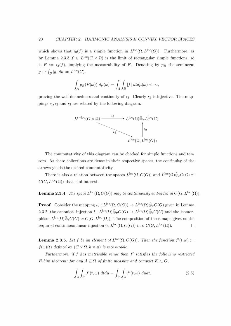
proving the well-definedness and continuity of ι3. Clearly ι3 is injective. The map-
pings ι1, ι2 and ι3 are related by the following diagram.
Lr−loc(G× Ω)
Lloc(Ω, Lloc(G))
Lloc(Ω)⊗πLloc(G)ι1
ι2ι3
The commutativity of this diagram can be checked for simple functions and ten-
sors. As these collections are dense in their respective spaces, the continuity of the
arrows yields the desired commutativity.
There is also a relation between the spaces Lloc(Ω, C(G)) and Lloc(Ω)⊗εC(G) 'C(G,Lloc(Ω)) that is of interest.
Lemma 2.3.4. The space Lloc(Ω, C(G)) may be continuously embedded in C(G,Lloc(Ω)).
Proof. Consider the mapping ι2 : Lloc(Ω, C(G))→ Lloc(Ω)⊗πC(G) given in Lemma
2.3.2, the canonical injection i : Lloc(Ω)⊗πC(G) → Lloc(Ω)⊗εC(G) and the isomor-
phism Lloc(Ω)⊗εC(G) ' C(G,Lloc(Ω)). The composition of these maps gives us the
required continuous linear injection of Lloc(Ω, C(G)) into C(G,Lloc(Ω)).
Lemma 2.3.5. Let f be an element of Lloc(Ω, C(G)). Then the function f ′(t, ω) :=
f(ω)(t) defined on (G× Ω, h× µ) is measurable.
Furthermore, if f has metrisable range then f ′ satisfies the following restricted
Fubini theorem: for any A ⊆ Ω of finite measure and compact K ⊂ G,∫A
∫Kf ′(t, ω) dtdµ =
∫K
∫Af ′(t, ω) dµdt. (2.5)

2.3. PRODUCT SPACES VIA VECTOR-VALUED MEASURE THEORY 21
Proof. The function f is measurable, which means by definition that there is a
sequence (fn) of C(G)-valued simple functions converging µ-a.e. to f . For a C(G)-
valued simple function g, the function g′(t, ω) := g(ω)(t) is easily seen to be measur-
able.
Now for µ-a.e. ω ∈ Ω, fn(ω) → f(ω) in C(G). In particular, for any t ∈ G,
fn(ω)(t) → f(ω)(t). This is synonymous with the expression f ′n(t, ω) → f ′(t, ω),
which implies the measurability of f ′.
We turn now to the Fubini-type result. Let M be the subspace (in the rela-
tive topology) of all elements in Lloc(Ω, C(G)) with metrisable range. Consider the
following diagram.
M
Lloc(Ω)
C(G)
C
∫A
∫K
∫A
∫K
HereA is a subset of Ω of finite measure andK is a compact subset ofG. The maps
are naturally defined:∫A : Lloc(Ω, C(G)) → C(G) sends an F to
∫A F (ω) dµ which
is well-defined because of the local integrability of F ;∫K : Lloc(Ω, C(G)) → Lloc(Ω)
sends an F to F (ω) :=∫K F (ω) dh. The well-definedness of this map depends on
the Pettis Measurability Theorem 2.2.1, because the functional f 7→∫K f dt is a
continuous linear functional on C(G). The maps∫A : Lloc(Ω)→ C and
∫K : C(G)→
C are defined in the obvious way.
So the arrows of the diagram are all continuous linear mappings. It is easy to see
that the diagram commutes for all simple functions in Lloc(Ω, C(G)). As the simple
functions form a dense subset, the commutativity of the diagram and the validity of
(2.5) is proved.
Alternatively, in the case that G is second countable, one can use the following
lemma to prove the measurability of f ′. It is an extension of [42, Ch. 7, exercise
8a)]. One of the reasons for including this result is to contrast the direct approach
in measure theory with our approach of using vector valued measure theory. Indeed
the previous lemma is stronger than the next one.
22 CHAPTER 2. HARMONIC ANALYSIS & CONVEX VECTOR SPACES
Lemma 2.3.6. Let X be a second countable metric space with Borel σ-algebra ΣX
and Y a measure space with σ-algebra ΣY . Let f be a complex-valued function defined
on X × Y . Suppose that for almost every x ∈ X, the cross sections fx(y) := f(x, y)
are measurable and that for almost every y ∈ Y the cross sections fy(x) := f(x, y) are
continuous. Then f is measurable with respect to the σ-algebra generated by ΣX×ΣY .
Proof. We shall suppose, without loss of generality, that f is real-valued. For any
a ∈ R, we must show that f−1[a,∞) is a measurable subset of X × Y . We do this
by constructing measurable subsets En,m ⊂ X × Y for all m,n ∈ N such that⋃n∈N
⋂m∈N
Em,n = f−1[a,∞).
For the remainder of the proof, let Q be a countable dense subset of X. For
each n ∈ N, let Vi be the open ball of radius 1/2n centred on qi ∈ Q. Define
An to be the countable collection of pairwise disjoint measurable subsets of X with
nonempty interior of diameter less than 1/n where we set A1 = V1 and for i > 1, set
Ai = Vi\(A1⋃. . .⋃An−1). We remove empty sets and renumber if necessary.
Now for any A ∈ An, let fA be a function on Y defined by
fA(y) = infq∈Q
⋂Afq(y) = inf
q∈Q⋂Af(q, y).
As fA the the infimum of a countable collection of measurable functions, it is itself
measurable.
For any m,n ∈ N we define
Em,n =⋃
A∈An
A× f−1A
[a− 1
m,∞),
which is clearly a measurable subset of X × Y . We shall show that⋃n∈N
⋂m∈N
En,m ⊆
f−1[a,∞).
If (x, y) ∈⋃n∈N
⋂m∈NEn,m, then for some n and all m, (x, y) ∈ En,m. Now x ∈ A
for some A ∈ An. For any q ∈ A⋂Q, fq ≥ fA, so
f−1q
[a− 1
m,∞)⊇ f−1
A
[a− 1
m,∞)
for all m ∈ N. Therefore fA(y) ≥ a− 1/m and so fq(y) ≥ a− 1/m for all q ∈ A⋂Q
and m ∈ N. As some subsequence in Q⋂A converges to x and as fy is continuous

2.4. HARMONIC ANALYSIS 23
on X, this means that f(x, y) ≥ a − 1/m for all m ∈ N. Hence f(x, y) ≥ a and
(x, y) ∈ f−1[a,∞).
Now we complete the proof by demonstrating the reverse inclusion f−1[a,∞) ⊆⋃n∈N
⋂m∈N
En,m. If (x, y) ∈ f−1[a,∞), then for any m ∈ N, f(x, y) > a − 1/m. Hence
if we set U = ω : f(ω, y) > a− 1/m, then U is an open subset of X, owing to the
continuity of fy. Clearly x ∈ U . Let n ∈ N be a number such that d(x, U c) > 1/n.
Note that x ∈ A for some A ∈ A2n.
In fact A ⊂ U , because for any a ∈ A and u′ ∈ U c,
d(a, u′) +1
2n≥ d(a, u′) + d(a, x) ≥ d(x, u′) >
1
n.
Hence d(a, u′) > 1/2n for all u′ ∈ U c, so a /∈ U c: that is, a ∈ U . Consequently,
fA(y) = infq∈A
⋂Qfq(y) ≥ a − 1/m, so (x, y) ∈ A × f−1
A [a − 1/m,∞). Therefore
(x, y) ∈ E2n,m for all m ∈ N and so (x, y) ∈⋃n∈N
⋂m∈N
En,m, proving the lemma.
All the different integrability conditions used in this section can be unified by the
following concept. Let (Ω,Σ, µ) be a measure space and let A ⊂ Σ be an algebra of
measurable sets. A measurable function f on Ω is called A-integrable if∫A|f | dµ
is finite for every A ∈ A. On the product space (Ω1×Ω2,Σ1×Σ2, µ1×µ2), when A is
the algebra of rectangles A×B where A and B have finite measure, the A-integrable
functions on Ω1 × Ω2 are the rectangular locally integrable functions. On G × Ω,
where A consists of all rectangles K × A where K ⊂ G is compact and A ⊂ Ω has
finite measure, the functions considered in Lemma 2.3.5 are A-measurable.
2.4 Harmonic Analysis
We develop here the harmonic analysis of abelian locally compact Hausdorff groups
that we shall require for the mean ergodic theory. Thereafter, we discuss some locally
convex topologies on vector spaces.
By M(G) we shall mean the Banach *-algebra of all finite Radon measures on G,
where the multiplication of measures is given by their convolution. The closed ideal
of all those measures absolutely continuous with respect to the Haar measure is the

24 CHAPTER 2. HARMONIC ANALYSIS & CONVEX VECTOR SPACES
Banach algebra L1(G). By G we shall mean the Pontryagin dual of G consisting of
all continuous characters of G; we will call continuous characters simply ‘characters’
in what follows. We denote by µ the Fourier transform of a measure µ ∈M(G) and
by ν(µ) = ξ ∈ G : µ(ξ) = 0 the null-set of µ.
We will need some results concerning the convergence of measures given the con-
vergence of their Fourier series. We recall some elements of the representation theory
of groups, as presented in Chapter 3 of [17]. We denote by P ⊂ Cb(G) the set of con-
tinuous functions of positive type. Such functions are also known as positive-definite
functions. (See [17] for the theory of functions of positive type, and both [17] and
[41] for material on positive-definite functions.)
Set P0 = φ ∈ P : ‖φ‖∞ ≤ 1. This set, viewed as a subset of the unit ball of
L1(G)∗, is weak*-compact.
We have the following extension of [41, Theorem 1.9.2]:
Theorem 2.4.1. Let (µn) be a bounded sequence of Radon measures on G and let K
be a closed subset of G, such that K is the closure of its interior. If (µn) converges
uniformly on compact subsets of K to a function φ, then there is a bounded Radon
measure µ such that µ = φ on K.
Proof. Without loss of generality, we may assume that (µn) ⊂ M+1 (G), the set of
positive Radon measures of norm no greater than 1. Also, for those closed K ⊂ G as
in the hypotheses, the space Cb(K) may be identified with a norm-closed subspace
of L∞(K,m), where m is the Haar measure on G. In the sequel, all L∞-spaces will
be taken with respect to the Haar measure and so we shall simply write L∞(K) for
L∞(K,m).
First we prove the result for compact K. Note that P0 ⊂ Cb(G), which can
be identified with a closed subset of L∞(G). Furthermore, P0 is absolutely convex
and closed in the weak*-topology on L∞(G) and hence closed in the finer norm
topology. Now consider the restriction map R : L∞(G) → L∞(K). This map is not
only norm-continuous, but weak*-continuous. Hence R(P0) is weak*-compact and
absolutely convex in L∞(K), which implies that it is also norm-closed (This follows
from [39, Prop. 8, e34] and the fact that the weak* and norm topologies on L∞(G)
are respectively the topologies σ(L∞(G), L1(G)) and β(L∞(G), L1(G))) . Of course,
R(P0) ⊂ C(K), which can be identified with a closed subset of L∞(K).
By Bochner’s Theorem (cf [41] or [17]), the Fourier transform gives a bijection

2.4. HARMONIC ANALYSIS 25
between M+1 (G) and P0(G). This means that (µn|K) ⊂ R(P0). By hypothesis, this
sequence converges uniformly to some φ ∈ R(P0) and so there is a φ ∈ P0 such that
R(φ) = φ. Consequently there is a µ ∈M+1 (G) such that µ = φ and so µ|K = φ.
This proves the result when K is compact. To prove it in the general case when
K is closed, we use the above result as well as the fact that Bochner’s Theorem states
that the Fourier transform is in fact a homeomorphism when M+1 (G) and P0(G) are
each given their weak*-topologies.
As (µn|K) is bounded and converges uniformly on compact subsets of K, its limit
φ is continuous and bounded on K. Let C be the collection of all compact subsets of
K which are the closures of their interiors. For any C ∈ C, define
S(C, φ) = µ ∈M+1 (G) : µ|C = φ|C ⊂M+
1 (G).
As proved above, S(C, φ) is nonempty. Furthermore, S(C, φ) is a weak*-compact
subset of M+1 (G). To see this, set
BC(φ) = f ∈ L∞(G) : f |C = φ|C a.e.
and note that BC(φ) is weak*-closed. Hence P0 ∩ BC(φ) is weak*-compact. Finally
P0 ∩BC(φ) is the image of S(C, φ) under the Fourier transform, so S(C, φ) must be
weak*-compact as well, by Bochner’s Theorem.
Now the collection S(C, φ) : C ∈ C is a collection of nonempty weak*-compact
subsets of M+1 (G). This collection has the finite intersection property, because if
C1, C2, . . . , Cn ∈ C, then
S(C1, φ) ∩ S(C2, φ) ∩ . . . ∩ S(Cn, φ) = S(C1 ∪ C2 ∪ . . . ∪ Cn, φ),
which is of course also nonempty. Hence the intersection of all the sets S(C, φ) is
nonempty. Let µ be in this intersection.
Then µ|C = φ|C for every C ∈ C; hence µ|K = φ.
We take the opportunity to demonstrate the power of the techniques developed
for constructing various topologies on vector spaces. Indeed, one can build such a
topology to encode the convergence of Fourier transforms handled in the last result.
Recall that G[, the Bohr compactification of G, is a compact group in which
G can be embedded continuously. It is constructed by first considering G under
the discrete topology. (This is denoted Gd.) The Pontryagin dual of this discrete

26 CHAPTER 2. HARMONIC ANALYSIS & CONVEX VECTOR SPACES
group is a compact group, namely G[. Recall also that AP (G), the set of almost
periodic functions on G, is simply the norm-closure in Cb(G) of all the trigonometric
polynomials. It so happens that AP (G) is precisely the set of continuous bounded
functions on G that can be extended to continuous functions on G[. So M(G[) is the
dual of AP (G) = C(G[).
By [41, Theorem 1.9.1], M(G) may be identified with a subspace of M(G[).
Theorem 2.4.2. Let (µn) be a bounded sequence of Radon measures on G such that
(µn) converges pointwise. Then (µn) is Cauchy in the σ(M(G), AP (G))-topology.
The sequence has a limit point in M(G[).
In particular, if (µn) converges uniformly on compact subsets of G, then (µn) is
convergent in M(G).
Proof. Let Φ(ξ) = limn→∞ µn(ξ) for all ξ ∈ G. By the Fourier Uniqueness Theorem,
there is a measure on G[, say µ, such that µ = Φ. Note that the σ(M(G), AP (G))-
topology is exactly the restriction of the weak*-topology on M(G[) to M(G). Define
D(G) to be the collection of all finite linear combinations of all Dirac measures on
G. Then the pair (C(Gd), D(G)) is a dual pair, where Gd has the discrete topology.
The Fourier transform F : M(G[) → C(Gd) has transpose F ′ : D(G) → AP (G). So
by [38], F is weakly convergent in this topology.
Now (µn) is relatively weak*-compact in M(G[) because this sequence is norm-
bounded. It has a convergent subsequence, (µnk). But then (µnk) is convergent in
M(Gd) in the σ(M(Gd), D(G))-topology, which means that (µnk) converges pointwise
on G to Φ. Hence µnk → µ. As all convergent subsequences of (µn) have the same
limit point, (µn) is convergent to a point in M(G[). It follows at once that (µn) is
Cauchy in the σ(M(G), AP (G))-topology.
For the second part of the theorem, note that by 2.4.1, the limit µ constructed
above belongs in fact to M(G).
There is an ideal of L1(G) that will be important for our purposes: K(G), the
set of all functions in L1(G) whose Fourier transforms have compact support. In [17]
and [41], it is shown that the ideal K(G) is a norm-dense subset of L1(G).
Turning to closed ideals I of L1(G), we can define the null-set ν(I) as we did for
individual functions and measures:
ν(I) = ξ ∈ G : f(ξ) = 0, for all f ∈ I.

2.4. HARMONIC ANALYSIS 27
Thus to each closed ideal in L1(G) we can assign a unique closed subset of G.
However the converse is not in general true: for a closed subset K of G, there is
usually more than one ideal whose null-set is K. Among all such ideals, two can be
singled out: the largest, ι+(K) consisting of all f ∈ L1(G) such that f is 0 on K,
and the smallest, ι−(K), consisting of all f ∈ L1(G) such that f is 0 on some open
neighbourhood of K. From the definitions, it is clear that ι−(K) ⊆ ι+(K). In [17]
and [41] it is proved that if I is a closed ideal in L1(G) with ν(I) = K, then
ι−(K) ⊆ I ⊆ ι+(K).
There are some sets K for which there is only one associated ideal. Such closed
sets are called sets of synthesis, or S-sets for short. In this case, we shall call ι(K)
the unique ideal associated with the S-set K. The fact that such sets have only one
closed ideal in L1(G) associated with them will be used often in what follows.
Spectral synthesis will play a large part in the sequel. References for this material
are [41, §7.8] and [17, §4.6]. To fix notation, we make a few remarks here. Any
weak*-closed translation-invariant subset T of L∞(G) has a spectrum, denoted σ(T ),
consisting of all characters contained in T . The spectrum is always closed in G.
The following theorem is crucial in the use of spectral synthesis. It is a slight
restatement of [21, Theoreme F, p132]. The second part is proved in [41, Theorem
7.8.2e)] (in [17, Proposition 4.75], a special case is shown.)
Theorem 2.4.3. (Spectral Approximation Theorem) Let V be a weak*-closed
translation-invariant subspace of L∞(G) with spectrum σ(V ) = Λ. Then for any
open set U containing Λ, any f ∈ V can be weak*-approximated by trigonometric
polynomials formed from elements of U .
Furthermore, if Λ is an S-set, then any f ∈ V can be weak*-approximated by
trigonometric polynomials formed from elements of Λ.
We need the following modification of [21, Theoreme A, p124].
Theorem 2.4.4. Let K be a compact subset of G and let µ be a measure in M(G)
whose Fourier transform µ does not vanish on K. Then there exists a g ∈ L1(G)
satisfying g(ξ) =1
µ(ξ)for all ξ ∈ K.

28 CHAPTER 2. HARMONIC ANALYSIS & CONVEX VECTOR SPACES
Proof. By [17, Lemma 4.50] or [41, Theorem 2.6.2], there exists a summable h on
G such that h = 1 on K. As µ ∗ h ∈ L1(G), we can apply [21, Theoreme A, p124] to
obtain a g ∈ L1(G) such that
g(ξ) =1
µ ∗ h(ξ)
for all ξ ∈ K. From the above equation and the fact that h = 1 on K, we see that
this g is the one required.
As with Theorem 2.4.1, we will often be in a position where we must infer proper-
ties of a summable function µ from knowledge of its Fourier transform on a compact
subset K ⊂ G. Of course, there will be in general many functions whose Fourier
transforms agree on K.
To clarify the situation, we make use of a quotient space construction. Using
ι+(K), the largest ideal with nullset K, we can form the quotient L1(G)/ι+(K). Let
[µ] denote an element of this quotient; it is an equivalence class consisting of all
functions ν such that µ|K = ν|K .
The following lemma exemplifies some of the techniques employed when working
with quotient spaces of L1(G), and will come in handy when proving the main result,
Theorem 4.3.1.
Lemma 2.4.5. Let (ϕn) be a sequence in L1(G) and let K be a compact subset of G.
If ([ϕn]) ⊂ L1(G)/ι+(K) is a relatively weakly compact sequence and limn→∞ ϕn(ξ)
exists for each ξ ∈ K, then ([ϕn]) is weakly convergent.
Proof. Suppose ([ϕn]) was not weakly convergent. Being relatively weakly compact,
it must then contain two weakly convergent subsequences ([ϕnk ]) and ([ϕn` ]) with
different limits [µ] and [ν] respectively.
The Gelfand transform FK : L1(G)/ι+(K)→ C(K), given by ϕ 7→ ϕ|K , is norm-
continuous and hence weakly continuous. Therefore (ϕnk) and (ϕn`) are weakly
convergent in C(K). By [13, Ch VII, Theorem 2], this means that limk→∞ ϕnk(ξ) =
µ(ξ) and lim`→∞ ϕn`(ξ) = ν(ξ). By hypothesis, then, µ = ν on K and so [µ] = [ν] in
L1(G)/ι+(K), a contradiction. Hence ([ϕn]) is weakly convergent.
We are also able to prove an interesting result that sheds light on the topological
vector space structure of the space L1(G)/ι+(K), a space which lies at the heart of
our Tauberian theorems. This result, Theorem 2.4.7, will not have a direct influence
on our work, but serves to illustrate the richness of the vector spaces that emerge

2.4. HARMONIC ANALYSIS 29
from harmonic analytic considerations. The next Lemma appears in [43, Theorem
4.9]. We state it here for completeness.
Lemma 2.4.6. Let E be a Banach space with dual E′ and let A ⊂ E be a closed
subspace. Then the dual of A may be identified with E′/A.
It is well known that A′ = E′/A⊥. Since A is a linear subspace, it is moreover
easy to verify that A⊥ = A.
The above result inspires the following proof.
Theorem 2.4.7. If K is a compact subset of G, then L1(G)/ι+(K) is the dual of
spf : f ∈ L1(G), supp f ⊂ K.
Proof. Note that C0(G)∗ = M(G) and set
A = spf : f ∈ L1(G), supp f ⊂ K ⊂ C0(G)
MK(G) = µ ∈M(G) : µ ≡ 0 on K.
We start by showing that A = MK(G). For any f ∈ L1(G) and µ ∈ M(G), we
compute:
〈f , µ〉 =
∫Gf dµ
=
∫G
∫Gf(ξ)〈ξ, x〉 dξdµ
=
∫Gf(ξ)
∫G〈ξ, x〉 dµdξ
=
∫Gf(ξ)µ dξ.
So if 〈f , µ〉 = 0 for all f ∈ A, then µ ≡ 0 on K. So MK(G) ⊃ A. On the other
hand, if µ ∈ MK(G), then by the above calculation 〈f , µ〉 = 0 for all f ∈ A and so
µ ∈ A.Consequently, by Lemma 2.4.6, A 'M(G)/MK(G). All that remains is to show
that M(G)/MK(G) ' L1(G)/ι+(K).
Consider the inclusion map i : L1(G)→M(G) and the quotient map q : M(G)→M(G)/MK(G). Let T = q i. We shall prove two things: T is surjective and ker
T = ι+(K). Together, this means that
L1(G)/ι+(K) 'M(G)/MK(G).

30 CHAPTER 2. HARMONIC ANALYSIS & CONVEX VECTOR SPACES
First T is surjective: let h ∈ L1(G) such that h ≡ 1 on K. For any µ ∈ M(G),
µ − µ ∗ h ∈ MK(G), so [µ] = [µ ∗ h] ∈ M(G)/MK(G). But now µ ∗ h ∈ L1(G), and
T (µ ∗ h) = [µ].
Next, we compute the kernel of T . If f ∈ ι+(K), then f ≡ 0 on K, so f ∈MK(G).
Hence ι+(K) ⊂ ker T . On the other hand, if f ∈ ker T , then f ∈MK(G) by definition
of T . So f ∈ ι+(K).

Chapter 3
Rearrangement invariant
Banach function spaces
This Chapter is about function spaces, in particular rearrangement invariant Banach
function spaces. The main reference works that set out the theory in detail include
especially Bennett and Sharpley [4], but also O’Neil [33] and Sharpley [46]. Rao and
Ren focus on the important subclass of Orlicz spaces in their book [37]. Section 3.1
deals with some basic definitions.
We focus on the fundamental function associated with a Banach function space
in Sections 3.2 and 3.3, as well as certain canonically constructed function spaces
derived from them. Using these spaces we can define the so-called weak type of an
operator, which is crucial for understanding the concept of a maximal inequality in
Chapter 5.
When working out the Transfer Principle and pointwise ergodic theorems, we
will need the integral estimates of Section 3.4. These results, requiring the measure
theoretic understanding of products of measure spaces gained in the previous Chapter,
plus the knowledge of functions spaces from Section 3.1, form the technical heart of
the work on the Transfer Principle and pointwise theorems.
3.1 Basic definitions and constructions
We start by recalling the definition of a rearrangement invariant Banach function
space (hereafter referred to as a r.i. BFS) over a resonant measure space (Ω, µ). Our
31
32 CHAPTER 3. BANACH FUNCTION SPACES
source for this material is mainly [4], and also [33].
Recall first that given a µ-a.e. finite measurable function f on (Ω, µ), the distri-
bution function s 7→ m(f, s) is defined by
m(f, s) = µ(ω ∈ Ω : |f(ω)| > s)
for all s ≥ 0. The decreasing rearrangement f∗ is defined as
f∗(s) = inft : m(f, t) ≤ s.
Two measurable functions f and g are equimeasurable if we have m(f, s) = m(g, s)
for all s ≥ 0. Note that the equimeasurability of f and g is the same as stating that
f∗(t) = g∗(t) for all t ≥ 0. By [4, Definition 2.2.3], the space (Ω, µ) is said to be
resonant if for each measurable finite a.e. functions f and g, the identity∫ ∞0
f∗(t)g∗(t) dt = sup
∫Ω|fg| dµ
holds as g ranges over all functions equimeasurable with g. As a special case of [4,
Theorem 2.2.6], let us mention that σ-finite nonatomic measure spaces and completely
atomic measure spaces, with all atoms having the same measure, are resonant.
One also defines a primitive maximal operator f 7→ f∗∗ as
f∗∗(s) =1
s
∫ s
0f∗(t) dt.
We call f∗∗ the double decreasing rearrangement of f .
When the function norm ρ that defines a Banach function space has the property
that ρ(f) = ρ(g) for all equimeasurable functions f and g, the Banach space is called
rearrangement invariant - see [4, Definitions 1.1, 4.1].
For any r.i. BFS X we define another r.i. BFS X ′, called the associate space, to
be the subset of the a.e.-finite measurable functions f on (Ω, µ) for which ‖f‖X′ is
finite, where
‖f‖X′ = sup∣∣ ∫
Ωf(ω)g(ω) dµ(ω)
∣∣ : g ∈ X, ‖g‖X ≤ 1.
We shall also have need of another Banach space Xb ⊆ X, which is the closure in
X of the set of all simple functions in X. This is not in general a r.i. BFS itself, but
is useful for the role it plays in the duality theory.
3.1. BASIC DEFINITIONS AND CONSTRUCTIONS 33
Associated with any rearrangement invariant BFS X, there is a fundamental
function ϕX : [0,∞)→ [0,∞) defined by
ϕX(t) = ‖χE‖X ,
where E is any subset of Ω such that µ(E) = t. By the rearrangement invariance
of X, this function is well-defined. It is a quasi-concave function, as explained in [4,
Definition 2.5.6]. Such functions are automatically continuous on (0,∞), as proved
in [4, Corollary 2.5.3]. They also have the following useful property.
Lemma 3.1.1. Quasiconcave functions are subadditive.
Proof. Indeed, if s ≤ t are two nonnegative real numbers, the fact that the mapping
t 7→ ϕ(t)
tis nonincreasing implies that
ϕ(s+ t)
s+ t≤ ϕ(t)
t≤ ϕ(s)
s
ϕ(s+ t) ≤(1 +
s
t
)ϕ(t)
= ϕ(t) +ϕ(t)
ts
≤ ϕ(t) + ϕ(s).
We denote by ϕ∗X the associate fundamental function of ϕX , where ϕ∗X = ϕX′ .
We shall often make use of the identity
ϕX(t)ϕ∗X(t) = t
for all t ≥ 0, as proved in [4, Theorem 2.5.2].
Recall that a Young’s function is a convex, nondecreasing function Φ : [0,∞] →[0,∞] for which Φ(0) = 0, limx→∞Φ(x) = ∞ and which is neither identically zero
nor infinite valued on all of (0,∞).
One class of spaces that we shall study is that of Orlicz spaces. The theory of
these important spaces, which include the standard Lp-spaces, is developed in [37].
In [4] and [33], they are also studied in some depth. We bring to mind the most
salient features of their construction. The Luxemburg norm ‖ · ‖L(Φ) is defined by a
Minkowski functional on the set of all finite a.e. measurable functions on (Ω, µ) by
the formula
‖f‖L(Φ) = infk−1 :
∫Ω
Φ(k|f |) dµ ≤ 1.

34 CHAPTER 3. BANACH FUNCTION SPACES
The set of all f for which ‖f‖L(Φ) <∞ is the Orlicz space L(Φ).
By [4, Theorem 2.5.13], for any rearrangement invariant Banach function space
X we have the embeddings
Λ(X) → X →M(X)
where the embeddings have norm 1.
There is also another Young’s function, called the complementary Young’s func-
tion. This is the function Ψ defined by
Ψ(x) = supy>0xy − Φ(y).
Using this complementary Young’s function, it is possible to define another, equiva-
lent norm on the Orlicz space L(Φ). To this end, define the Orlicz norm ‖ · ‖L(Φ) on
the space of measurable functions f on (Ω, µ) by setting
‖f‖L(Φ) = sup∫ ∞
0f∗(s)g∗(s) ds : ‖g‖L(Ψ) ≤ 1
. (3.1)
Now the Orlicz and Luxemburg norms on the Orlicz space L(Φ) are equivalent.
In fact it is proved in [4, Theorem 4.8.14] that
‖f‖L(Φ) ≤ ‖f‖L(Φ) ≤ 2‖f‖L(Φ). (3.2)
We shall often have need of the inverse of Young’s functions and (less frequently)
fundamental functions. The following definition makes the notion precise.
Definition 3.1.2. Let ϕ : R+ → R+ be a monotone left-continuous function. for
any t ∈ R+, we form the sets St = x : ϕ(x) ≤ t and It = x : ϕ(x) > t. These
sets form a Dedekind cut of R+ and we define ϕ−1(t) to number determined by this
cut.
Hence we may write ϕ−1(t) = supSt = inf It if ϕ is nonincreasing.
Now for an Orlicz space L(Φ) equipped with the Luxemburg norm, its fundamen-
tal function ϕ is related to Φ by the equation
ϕ(t) = 1/Φ−1(1/t) (3.3)
for all 0 < t ≤ |Ω| as shown in [4, Lemma 4.8.17]. In the sequel, given a Young’s
function Φ we define the fundamental function associated to Φ to be the quasconcave
function defined by (3.3).

3.1. BASIC DEFINITIONS AND CONSTRUCTIONS 35
Given a r.i. BFS X over (Ω, µ), we canonically associate two other r.i. BFSs with
X, apart from the Orlicz space. If ϕX is the fundamental function associated with
X, define the first space M(X) to consist of all the measurable functions f over Ω
such that
‖f‖M(X) = sups>0
f∗∗(s)ϕX(s) <∞.
The space M(X) is a Banach space with the norm ‖ · ‖M(X). This is the largest r.i.
BFS with fundamental function ϕX . In other words, if Y is any other r.i. BFS with
fundamental function ϕX , then Y is contractively embedded in M(X). Note that as
the quasiconcave function ϕX is the only property of X required to construct M(X),
we may just as well denote this space by M(ϕX).
The second space is the associate of M(X ′). We define Λ(X) to consist of all
measurable functions f over Ω such that
‖f‖Λ(X) = sup∫ ∞
0f∗(s)g∗(s) ds : ‖g‖M(ϕ∗X) ≤ 1
<∞.
The set Λ(X) is a Banach space with norm ‖ · ‖Λ(X).
As in the case of M(X), we can just as well write Λ(ϕX), as ϕX is the only
property of X employed in the construction of Λ(X). This is the smallest r.i. BFS
with fundamental function ϕX ; if Y is any other r.i. BFS with this fundamental
function then there is a continuous injection of Λ(X) into Y .
There is another function space, denoted M∗(X), that can be constructed from
a given r.i. BFS X. Although complete, this space is in general not normable and
consists of all those finite a.e. measurable functions f on (Ω, µ) for which the quasi-
norm ‖ · ‖M∗(X) defined by
‖f‖M∗(X) = sups>0
f∗(s)ϕX(s)
is finite. Again, note that the only property of X required for this construction is
its fundamental function ϕX . While M∗(X) is not necessarily a Banach space, it is
a quasi-Banach space, in that ‖f‖M∗(X) = 0 if and only if f = 0 a.e., ‖λf‖M∗(X) =
|λ|‖f‖M∗(X) for all complex λ and
‖f + g‖M∗(X) ≤ 2(‖f‖M∗(X) + ‖g‖M∗(X))
for all f, g ∈M∗(X). This space was introduced in [46] - see also [4, Ch. 4, exercise
21].
We provide a useful equivalent definition of the M∗(X)-norm.

36 CHAPTER 3. BANACH FUNCTION SPACES
Lemma 3.1.3. If ϕ is a fundamental function, then supt>0
f∗(t)ϕ(t) = sups>0
sϕ(m(f, s)).
Proof. We follow [22, Proposition 1.4.5.16, p46]. Given s > 0, pick ε ∈ (0, s). As
f∗(m(f, s)− ε) > s,
supt>0
f∗(t)ϕ(t) ≥ f∗(m(f, s)− ε)ϕ(m(f, s)− ε) > sϕ(m(f, s)− ε).
Because ϕ is continuous on (0,∞), as ε→ 0, we obtain
supt>0
f∗(t)ϕ(t) ≥ sϕ(m(f, s))
for all s > 0, which proves that supt>0 f∗(t)ϕ(t) ≥ sups>0 sϕ(m(f, s)).
Conversely, given t > 0, if f∗(t) > 0 pick ε ∈ (0, f∗(t)). Then m(f, f∗(t)− ε)) > t,
meaning that
sups>0
sϕ(m(f, s)) ≥ (f∗(t)− ε)ϕ(m(f, f∗(t)− ε)).
As ϕ is nondecreasing, we have (f∗(t)−ε)ϕ(m(f, f∗(t)−ε)) ≥ (f∗(t)−ε)ϕ(t). Letting
ε→ 0, we obtain
sups>0
sϕ(m(f, s)) ≥ f∗(t)ϕ(t)
for all t > 0. If f∗(t) = 0, this inequality is trivially satisfied. Hence supt>0 f∗(t)ϕ(t) ≤
sups>0 sϕ(m(f, s)).
Let us make some remarks on operators between function spaces, in particular
on the weak type of an operator. There are two standard definitions of this concept.
Let X and Y be rearrangement invariant BFSs. We say that a sublinear operator T
has Marcinkiewicz weak type (X,Y ) if T maps X into M∗(Y ) and that T has Lorentz
weak type (X,Y ) if it maps Λ(X) into M∗(Y ). Clearly if T is of Marcinkiewicz weak
type (X,Y ) then it is of Lorentz weak type (X,Y ). In the sequel, we shall write
‘weak type’ for ‘Marcinkiewicz weak type.’
For an operator T of weak type (X,Y ) there exists a c > 0 such that ‖Tf‖M∗(Y ) ≤c‖f‖X . The smallest value of c for which this equation holds is called the norm of T .
As we shall mostly be working with Λ-, M - and Orlicz-spaces, let us fix some
terminology for dealing with the weak types associated with these kinds of spaces.
Definition 3.1.4. (Weak type) Let ΦA and ΦB be Young’s functions with associated
fundamental functions ϕA and ϕB respectively. We say that a sublinear operator T
has Λ-, M - or L-weak type (ϕA, ϕB) if it respectively maps Λ(ΦA), M(ΦA) or L(ΦA)
into M∗(ϕB).

3.2. MANIPULATIONS OF FUNDAMENTAL FUNCTIONS 37
Bear in mind that if an operator is of M -weak type (ϕA, ϕB), then it is automat-
ically of L- and Λ-weak types (ϕA, ϕB) too.
3.2 Manipulations of fundamental functions
It is known (cf. [4, Propositions 2.5.10, 2.5.11]) that a fundamental function may
be replaced with a concave fundamental function for most purposes. On the other
hand, a Young’s function is always convex, and if one considers (3.3), one sees that
the associated fundamental function is automatically concave. (In other words, if
we consider an Orlicz space with the Luxemburg norm, its fundamental function
is concave). This is a consequence of the next Lemma, which will also show how
in certain cases one can start with a fundamental function and associate with it a
Young’s function.
Lemma 3.2.1. Let ϕ : R+ → R+ be a nondecreasing convex (respectively concave)
function. Then ϕ−1 is nondecreasing and concave (respectively convex).
Furthermore, t 7→ 1/ϕ(1/t) is nondecreasing and convex (respectively concave).
Proof. Suppose that ϕ is convex, let x, y ∈ R+ and 0 ≤ λ ≤ 1. We define three
subsets of R+ as follows.
SΣ = s : ϕ(s) ≤ λx+ (1− λ)y
Sx = s : ϕ(s) ≤ x
Sy = s : ϕ(s) ≤ y.
Fix an ε > 0 and let tx ∈ Sx and ty ∈ Sy, with tx ≥ supSx−ε and ty ≥ supSy−ε.Then from the convexity of ϕ, we can estimate
ϕ(λtx + (1− λ)ty) ≤ λϕ(tx) + (1− λ)ϕ(ty)
≤ λx+ (1− λ)y.
Hence λtx+(1−λ)ty ∈ SΣ and supSΣ ≥ λ supSx+(1−λ) supSy−ε. As ε is arbitrary,
Definition 3.1.2 shows us that
ϕ−1(λx+ (1− λ)y) ≥ λϕ−1(x) + (1− λ)ϕ−1(y).
38 CHAPTER 3. BANACH FUNCTION SPACES
For the second part, suppose that ϕ is concave, and again that x, y ∈ R+ and
0 ≤ λ ≤ 1. We define three subsets of R+ as follows.
IΣ = s : ϕ(s) > λx+ (1− λ)y
Ix = s : ϕ(s) > x
Iy = s : ϕ(s) > y.
Fix an ε > 0 and let tx ∈ Sx and ty ∈ Sy, with tx ≤ inf Ix + ε and ty ≤ inf Iy + ε.
Then from the concavity of ϕ, we get that
ϕ(λtx + (1− λ)ty) ≥ λϕ(tx) + (1− λ)ϕ(ty)
> λx+ (1− λ)y.
Hence λtx + (1− λ)ty ∈ IΣ and inf IΣ ≤ λ inf Ix + (1− λ) inf Sy + ε. As ε is arbitrary,
the result follows as before.
To prove the second part of the lemma, let I(t) = 1/t for t > 0. set φ(t) =
I ϕ I(t). As concave and convex functions have derivatives in L1(R+), we may
compute:
φ′(t) = I ′(ϕ I)(t).ϕ′(I(t)).I ′(t)
= −(ϕ I)−2(t)ϕ′(1/t)(−t−2).
If ϕ is concave, then ϕ′ is nonincreasing, so t 7→ ϕ′(1/t) is nondecreasing. Clearly
t 7→ (−t−2)ϕ−2(1/t) is nondecreasing, because t 7→ ϕ(t)/t is nonincreasing. Hence φ′
is nondecreasing and so φ is concave.
If ϕ is convex, the same reasoning shows that φ is convex.
From this lemma, we immediately deduce that if ϕ is concave, then t 7→ 1/ϕ−1(1/t)
is convex. Moreover if limt→0 ϕ(t) = 0 and limt→∞ ϕ(t) = ∞, then 1/ϕ−1(1/t) is a
Young’s function.
Finally, to round off the results pertaining to the taking of inverses, we have the
following result on double inverses.
Lemma 3.2.2. Let ϕ be a nondecreasing function, either concave or convex, on
(0,∞). Then for all t > 0, (ϕ−1)−1(t) = ϕ(t).
Proof. We shall prove the result for ϕ concave on (0,∞); the proof in the convex
case is virtually identical. Let us define `0 = limt→0 ϕ(t) and `∞ = limt→∞ ϕ(t). If

3.3. COMPARISON OF FUNDAMENTAL FUNCTIONS 39
ϕ is constant on an interval [a, b) then ϕ is constant on [a,∞), for if z = ϕ(a) and
s = supξ : ϕ(ξ) = z < ∞, then for ε > 0 small enough, ϕ(a/2 + (s + ε)/2) <
ϕ(a)/2 + ϕ(s + ε)/2, contradicting the concavity of ϕ. With this in mind, define
s0 =∞ if ϕ is strictly increasing and s0 = infξ : ϕ(ξ) = `∞.The proof follows from studying the following two graphs.
`0
`∞
s0
ϕ
∞
s0
`∞`0
ϕ−1
Indeed, for all s > `∞, ϕ−1(s) = supt : ϕ(t) ≤ s = ∞. For all s ≤ `0,
ϕ−1(s) = inft : ϕ(t) > s = 0. Also, ϕ is injective on (0, s0] as it is strictly
increasing on this interval.
Hence (ϕ−1)−1(t) = ϕ(t) for all t ∈ (0, s0]. For t > s0, (ϕ−1)−1(t) = sups :
ϕ−1(s) ≤ t = `∞ = ϕ(t).
3.3 Comparison of fundamental functions
It should be quite clear that a lot rests upon the analysis of the various fundamental
functions associated with r.i. BFSs. Indeed, based on techniques for comparing qua-
siconcave functions developed in the sequel, we will derive our results on the weak
type of the transferred operator.
The growth properties of a Young’s function have great bearing on the properties
of the associated Orlicz space. The same holds more generally for the growth prop-
erties of a fundamental function and its associated BFSs. This part of the work will
be concerned with translating some standard growth conditions on Young’s functions
into conditions on fundamental functions. Then we shall analyse these conditions in
terms of inequalities prominent in O’Neil’s work [33].

40 CHAPTER 3. BANACH FUNCTION SPACES
Recall from [37] that a Young’s function Φ is said to satisfy the ∆2 condition
(globally), denoted Φ ∈ ∆2 (Φ ∈ ∆2 (globally)) if
Φ(2x) ≤ KΦ(x), x ≥ x0 ≥ 0 (x0 = 0)
for some absolute constant K > 0. The Young’s function Φ satisfies the ∇2 condition
(globally), denoted Φ ∈ ∇2 (Φ ∈ ∇2 (globally)) if
Φ(x) ≤ 1
2`Φ(`x), x ≥ x0 ≥ 0 (x0 = 0)
for some ` > 1.
We now state these definitions in terms of fundamental functions.
Definition 3.3.1. A fundamental function ϕ is said to satisfy the ∆2 condition
(globally), denoted ϕ ∈ ∆2 (ϕ ∈ ∆2 (globally)) if
ϕ(Kx) ≥ 2ϕ(x), x ≥ x0 ≥ 0 (x0 = 0) (3.4)
for some absolute constant K > 0.
A fundamental function ϕ is said to satisfy the ∇2 condition (globally), denoted
ϕ ∈ ∇2 (ϕ ∈ ∇2 (globally)) if
ϕ(x) ≥ 2
`ϕ(`x), x ≥ x0 ≥ 0 (x0 = 0) (3.5)
for some absolute constant ` > 1.
Suppose that ϕ satisfies the ∆2 condition. Note that as ϕ is nondecreasing, if
K < 1, then ϕ(Kx) ≤ ϕ(x), so 2ϕ(x) ≤ ϕ(x) for every x ≥ x0 - a contradiction as
ϕ(x) = 0 if and only if x = 0. Hence K ≥ 1. But then ϕ(Kx) ≤ Kϕ(x), which follows
from the nonincreasing behaviour of x 7→ ϕ(x)/x. Hence 2ϕ(x) ≤ ϕ(Kx) ≤ Kϕ(x).
This shows that K ≥ 2.
Likewise, we can provide a crude bound for ` in the case that ϕ satisfies the ∇2
condition. As ` > 1, ϕ(`x) ≥ ϕ(x) ≥ 2
`ϕ(`x) for every x ≥ x0, so 1 ≥ 2/`, which
implies that ` ≥ 2.
Note that the same reasoning applies to the selection of K and ` for Young’s
functions respectively satisfying the conditions ∆2 and ∇2. Indeed, let Φ ∈ ∆2. By
[37, Corollary I.3.2], we may write
Φ(x) =
∫ x
0φ(t) dt

3.3. COMPARISON OF FUNDAMENTAL FUNCTIONS 41
for some nondecreasing left continuous function φ : [0,∞)→ [0,∞] for which φ(0) =
0. Hence
Φ(2x) =
∫ x
0φ(t) dt+
∫ 2x
xφ(t) dt
≥∫ x
0φ(t) dt+
∫ x
0φ(t) dt
= 2Φ(x)
on account of the fact that φ is nondecreasing. Therefore 2Φ(x) ≤ Φ(2x) ≤ KΦ(x),
implying that K ≥ 2.
If Φ ∈ ∇2 and Φ(x) ≤ (1/2`)Φ(`x) for some ` < 2, note that by the convexity of
Φ and the identity Φ(0) = 0,
Φ(`x) = Φ((1− `/2)0 + (`/2)2x) ≤ `
2Φ(2x).
Consequently, Φ(x) ≤ (1/2`)Φ(`x) ≤ (1/2`)(`/2)Φ(2x) = (1/4)Φ(2x). So Φ satisfies
the ∇2 condition with ` = 2.
Proposition 3.3.2. Suppose that the quasiconcave function ϕ satisfies the ∆2 con-
dition globally. Then there exist constants 1 ≥ ε > 0 and A > 0 such that for all
y ≥ 1, 0 < p < ε and x ∈ R+,
ϕ(yx) ≥ Aypϕ(x).
Furthermore, if ϕ satisfies the ∇2 condition globally, then there exist constants
1 > ε ≥ 0 and B > 0 such that for all y ≥ 1, ε ≤ p < 1 and x ∈ R+, it holds that
ϕ(yx) ≤ Bypϕ(x).
Proof. Suppose that ϕ satisfies the ∆2 condition. As noted in the remarks preceding
this Proposition, we can choose a K ≥ 2 such that (3.4) holds. Set ε = ln 2/ lnK and
let y ≥ 1. By iterating the definition of the ∆2 condition, we see that for any n ∈ Nand x ≥ 0,
2nϕ(x) ≤ ϕ(Knx).
There is a natural number n such thatKn−1 ≤ y < Kn. Define λ such that y/Kn = λ.
Then 1/K ≤ λ < 1, which allows the following computation:
ϕ(yx) = ϕ(λKnx) ≥ λϕ(Knx)
≥ λ2nϕ(x). (3.6)

42 CHAPTER 3. BANACH FUNCTION SPACES
Now y/λ = Kn implies that n =ln y − lnλ
lnKand
2n = en ln 2 = eln ylnK
ln 2− lnλlnK
ln 2
2n = yln 2lnK λ−
ln 2lnK
λ2n = yln 2lnK λ1− ln 2
lnK .
Setting A = (1/K)1−ln 2/ lnK , we see that
λ2n ≥ Ayε. (3.7)
Combining (3.6) and (3.7), for any 0 < p < ε and y ≥ 1, we have
ϕ(yx) ≥ Aypϕ(x).
Now suppose that ϕ satisfies the ∇2 condition, that is, inequality (3.5) with
` ≥ 2. Define ε = 1− ln 2/ ln ` and let y ≥ 1. There is a natural number n such that
`n−1 ≤ y < `n. Set λ = y/`n. Then 1/` ≤ λ < 1 and
ϕ(yx) = ϕ(λ`nx) ≤ ϕ(`nx)
≤ `n
2nϕ(x). (3.8)
Now n =ln y − lnλ
ln `, so
`n
2n= en ln `−n ln 2 = eln y−lnλ−(ln y−lnλ) ln 2
ln `
= e
(1− ln 2
ln `
)ln y/λ
= y1− ln 2ln ` λ
ln 2ln `−1. (3.9)
Because 0 < ln 2/ ln ` ≤ 1 and 1/` ≤ λ < 1, we have that λln 2/ ln `−1 ≤ `1−ln 2/ ln `.
Hence for any 1 > p ≥ 1− ln 2/ ln ` = ε, from (3.9) we have
`n
2n≤ Byp,
where B = `1−ln 2/ ln `. Substituting this into (3.8) yields the result.
The inequalities ϕ(yx) ≥ Aypϕ(x) and ϕ(yx) ≤ Bypϕ(x) obtained in the Propo-
sition above are instances of tail growth conditions: they are valid for y large enough.
A larger class of fundamental functions satisfying such conditions is provided in [46],
which we now recall.

3.3. COMPARISON OF FUNDAMENTAL FUNCTIONS 43
Definition 3.3.3. We define two classes of fundamental functions as follows.
1. ϕ ∈ U if for some 0 < α < 1, there are positive constants A and δ such that
ϕ(ts) ≤ Atαϕ(s) if t ≥ δ.
The U-index of ϕ, denoted ρϕU , is the infimum of all α for which the above
inequality obtains.
2. ϕ ∈ L if for some α > 0, there are positive constants A and δ such that
ϕ(ts) ≥ Atαϕ(s) if t ≥ δ.
The L-index of ϕ, denoted ρϕL, is the supremum of all α for which the above
inequality obtains.
We shall often require the equivalent forms of this definition as provided in the
next result.
Lemma 3.3.4. Let ϕ be a fundamental function.
1. ϕ ∈ U if and only if Aϕ(uv) ≥ vαϕ(u) for some constants A, δ > 0 and u >
0, v ≤ δ.
2. ϕ ∈ L if and only if Aϕ(uv) ≤ vαϕ(u) for some constants A, δ > 0 and u >
0, v ≤ δ.
Moreover, by adjusting A if necessary, we may always take δ = 1.
Proof. Suppose ϕ ∈ U so that ϕ(ts) ≤ Atαϕ(s) if t ≥ δ. By the change of variables
u = ts and v = 1/t, we get Aϕ(uv) ≥ vαϕ(u) for u > 0, v ≤ 1/δ. Part (2) is treated
with the same change of variables.
For the last part, suppose ϕ ∈ U so that ϕ(ts) ≤ Atαϕ(s) if t ≥ δ. If δ ≤ 1, then
this inequality is certainly true for all t ≥ 1. If δ > 1, then for all t ≥ 1, s > 0,
ϕ(ts) ≤ ϕ(δts) ≤ A(δt)αϕ(s)
because ϕ is nondecreasing. Setting A′ = Aδα, we have proven that ϕ(ts) ≤ A′tαϕ(s)
if t ≥ 1. The same reasoning can be used for the case ϕ ∈ L.
We have thus shown that U and L defined above are identical to the classes as
defined in [46]. Furthermore, the U- and L- indices of ϕ are equal to the fundamental

44 CHAPTER 3. BANACH FUNCTION SPACES
indices introduced by Zippin and defined in [46]. We will prove this later in the
chapter.
Proposition 3.3.2 shows that if ϕ satisfies the ∆2 condition, then ϕ ∈ L and if ϕ
satisfies the ∇2 condition then ϕ ∈ U .
In a far-reaching extension of the U and L classes, we shall use relations between
three quasiconcave functions ϕA, ϕB and ϕC that satisfy one of the inequalities
ϕC(st) ≤ θϕA(t)ϕB(s) for all t, s > 0 (3.10)
ϕC(st) ≤ θϕA(t)ϕB(s), s > 0, t ≥ δ (3.11)
ϕC(st) ≤ θϕA(t)ϕB(s), s > 0, t ≤ δ (3.12)
for some δ > 0. Inequalities such as (3.10) are common and have been extensively
studied by O’Neil in [33] and [32].
The inequalities (3.11) and (3.12), which are more general that (3.10), shall be the
basis for our analysis of the maximal inequalities for a transfer operator. Note that
the classes U and L satisfy (3.11) and (3.12) respectively. Inequalities of these types
are common for fundamental functions. For example, note that for any quasiconcave
function ϕ we have
ϕ(st) ≤ ϕ(s)t
for all s > 0 and t ≥ 1, which is true because t 7→ ϕ(t)/t is nonincreasing. Another
general O’Neil-type inequality appears in Lemma 3.3.5.
We recall the construction of the Boyd indices of a r.i. BFS X which is defined by
a function norm ρ. First, by the Luxemburg Representation Theorem [4, Theorem
2.4.10] there is a (not necessarily unique) r.i. BFS X over the positive reals with
Lebesgue measure, defined by a function norm ρ which is related to ρ by the formula
ρ(f∗) = ρ(f)
for every f ∈ X. Now for each t ∈ R+ we define the dilation operator Et by
(Etg)(s) = g(st)
for all s ∈ R+ and g a measurable and finite a.e. function on [0,∞). Let hX(t)
denote the operator norm of E1/t: that is, hX(t) = ‖E1/t‖B(X) for t > 0. Define
hX(0) = 0. In [4, Section 3.5], the authors thoroughly develop the basics of the theory,
including the fact that hX is submultiplicative. Note that it is also quasiconcave, for

3.3. COMPARISON OF FUNDAMENTAL FUNCTIONS 45
by [4, Proposition 3.5.11], hX is nondecreasing and hX(t)/t = hX′(1/t), which is
nonincreasing. Furthermore, hX(t) > 0 for t > 0, which is a consequence of the next
Lemma. The Lemma also provides an interesting general example of the O’Neil-type
inequality (3.10).
Lemma 3.3.5. If X is a r.i. BFS then for all s, t > 0,
ϕX(st) ≤ hX(t)ϕX(s)
ϕX(st) ≥ h∗X′(t)ϕX(s).
Proof. Consider the function space X over the positive reals given by the Luxemburg
Representation Theorem mentioned above and fix s, t ∈ R+. Note that
ϕX(st) = ‖χ(0,st)‖X= ‖E1/tχ(0,s)‖X≤ ‖E1/t‖B(X)‖χ(0,s)‖X= hX(t)ϕX(s).
From this inequality, we immediately deduce that ϕ∗X(st) ≥ h∗X(t)ϕ∗X(s). As ϕ∗X =
ϕ′X , this can be written as ϕX′(st) ≥ h∗X(t)ϕX′(s). Equivalently, ϕX(st) ≥ h∗X′(t)ϕX(s).
It is worth mentioning that by [4, Proposition 3.5.11], h∗X′(t) = 1/hX(1/t). Note
also that as hX is submultiplicative, h∗X′ is supermultiplicative, in that h∗X′(st) ≥h∗X′(s)h
∗X′(t). We have shown that any fundamental function ϕX can be bounded
above by a submultiplicative and below by a supermultiplicative function (up to a
constant factor), in that
ϕ(1)h∗X′(t) ≤ ϕ(t) ≤ ϕ(1)hX(t).
The lower and and Boyd indices of X, denoted respectively by αX and αX are
given by
αX = limt→0+
lnhX(t)
ln t, αX = lim
t→∞
lnhX(t)
ln t.
For a r.i. BFS X with fundamental function ϕ, if M(t,X) = sups>0 ϕ(st)/ϕ(s),
recall than Zippin [50] defines the fundamental indices as
βX
= limt→0+
lnM(t,X)
ln t, βX = lim
t→∞
lnM(t,X)
ln t.

46 CHAPTER 3. BANACH FUNCTION SPACES
Recall from Definition 3.3.3 the definitions of the L- and U-indices of a funda-
mental function. Note that the fundamental indices of a fundamental function are
always defined, even if the L- or U- indices are not. The relation between the Boyd
and fundamental indices given in the next Lemma is well known - see for example [4,
Chapter 3, exercise 14].
Lemma 3.3.6. Let X be a r.i. BFS with fundamental function ϕ. Then
0 ≤ αX ≤ βX ≤ βX ≤ αX ≤ 1.
Moreover, ϕ ∈ U if and only if βX < 1 and in this case βX = ρϕU , and ϕ ∈ L if and
only if βX> 0 and in this case β
X= ρϕL.
Proof. From Lemma 3.3.5 it is easy to see that M(t,X) ≤ hX(t). Hence if t >
1, lnM(t,X)/ ln t ≤ lnhX(t)/ ln t, so βX ≤ αX . On the other hand, if t < 1,
lnM(t,X)/ ln t ≥ lnhX(t)/ ln t, so βX≥ αX . The fact that M(t,X) is nondecreasing
shows that βX≤ βX .
The rest of the Lemma follows directly from the definition of the U- and L-
indices.
3.4 Estimates of integrals and function norms
When working with maximal inequalities, there are certain integrals that we will need
to estimate. The following Proposition covers the cases that we will need.
First, some terminology, following [27]: consider a measure space (Ω,Σ, µ) and a
countable collection D ⊂ Σ of measurable subsets of µ-finite measure. The σ-algebra
σ(D) generated by D is contained in Σ. If for any F ∈ Σ there is a D ∈ σ(D)
such that F∆D has null measure, where F∆D denotes the symmetric difference
between D and F , we say that (Ω,Σ, µ) is countably generated modulo null sets, or
just countably generated. We call D the generators of Σ. Moreover, we may assume
that D is an algebra, for if D is countable, so is the algebra it generates. If D is an
algebra of sets that generates Σ in the above sense, it is easy to see that if F ⊂ Ω
is any µ-finite subset and ε > 0, then there is a D ∈ D such that µ(D∆F ) < ε and
|µ(D)− µ(F )| < ε.

3.4. ESTIMATES OF INTEGRALS AND FUNCTION NORMS 47
Proposition 3.4.1. Let (Ω1, µ1) and (Ω2, µ2) be resonant spaces with Ω2 countably
generated. Let ΦA,ΦB and ΦC be Young’s functions and ϕA, ϕB and ϕC be their
respective associated fundamental functions satisfying
θϕA(st) ≥ ϕB(s)ϕC(t) (3.13)
for all s, t > 0 and some θ > 0. Let f be a measurable function on Ω1 × Ω2 and
E ⊂ Ω1 a subset of finite measure.
1) If f ∈M(ΦA), then
ϕC(|E|)|E|
∫E‖fω1‖M(ΦB) dµ1(ω1) ≤ 4e3θ‖f‖M(ΦA).
2) If f ∈ Λ(ΦA) and limt→0 ϕ∗B(t) = 0, then
ϕC(|E|)|E|
∫E‖fω1‖Λ(ΦB) dµ1(ω1) ≤ 6θ‖f‖Λ(ΦA).
3) If f ∈ L(ΦA) and limt→0 ϕ∗B(t) = 0, then
ϕC(|E|)|E|
∫E‖fω1‖L(ΦB) dµ1(ω1) ≤ θ‖f‖L(ΦA).
This theorem is to some extent an adaptation of [33, Theorem 8.18] to the
needs of the present program. In particular here g is replaced by χE and h(ω) =∫f(ω1, ω2)g(ω2)dµ(ω2) by
∫‖fω1‖X(ΦB)dµ(ω2).
As the proof of this Proposition relies heavily on [33, Theorem 8.18], it is worth
mentioning that the condition on the fundamental functions given there, namely
Φ−1A (st)Φ−1
B (t) ≤ θtΦ−1C (s), can with the help of (3.3) and the identity ϕB(t)ϕ∗B(t) = t
be written in the equivalent form
θϕA(st) ≥ ϕ∗B(t)ϕC(s).
Proof. Let D be a countable algebra that generates (Ω2, µ2).
Suppose f ∈M(ΦA). For any subset ∆ ⊂ Ω2 of finite measure, define h∆ by
h∆(ω1) =1
ϕ∗B(|∆|)
∫∆|f(ω1, ω2)| dµ2(ω2).
Thus h∆(ω1) =
∫Ω2
|f |(ω1, ω2)(χ∆(ω2)/ϕ∗B(|∆|)) dµ2(ω2). Note that (3.13) can be
written in the form
θϕA(st) ≥ (ϕ∗B)∗(s)ϕC(t)

48 CHAPTER 3. BANACH FUNCTION SPACES
because for any fundamental function ϕ, (ϕ∗)∗ = ϕ. We apply [33, Theorem 8.18,
part 1] to conclude that h∆ ∈ M(ΦC), with ‖h∆‖M(ΦC) ≤ 4e3θ‖f‖M(ΦA). We also
used the obvious fact that ‖χ∆/(ϕ∗B(|∆|))‖Λ(ϕ∗B) = 1.
Now define
h = sup∆∈D
h∆.
As h is the supremum of a countable number of functions, it is itself a measurable
function.
For any ∆ ∈ D and µ1-almost every ω1 ∈ Ω1,
h(ω1) =1
ϕ∗B(|∆|)
∫∆|fω1 | dµ2 =
1
|∆|
∫∆|fω1 | dµ2.ϕB(|∆|)
≤ f∗∗ω1(|∆|)ϕB(|∆|) ≤ ‖fω1‖M(ΦB),
by definition of the norm ‖ · ‖M(ΦB). Hence h(ω1) ≤ ‖fω1‖M(ΦB) a.e.
On the other hand for any fixed ε > 0, there is a t > 0 such that f∗∗ω1(t)ϕB(t) >
‖fω1‖M(ΦB) − ε. As (Ω2, µ2) is a resonant space, by [4, Proposition 2.3.3], there is a
subset F such that |F | = t and
1
|F |
∫F|fω1 | dµ2 > f∗∗ω1
(t)− ε/ϕB(t).
Hence1
ϕ∗B(|F |)
∫F|fω1 | dµ2 > f∗∗ω1
(t)ϕB(t)− ε.
Because D is dense in the Borel σ-algebra, there is a ∆ ∈ D such that∣∣∣∣ 1
ϕ∗B(|∆|)
∫∆|fω1 | dµ2 −
1
ϕ∗B(|F |)
∫F|fω1 | dµ2
∣∣∣∣ < ε.
Therefore
h∆(ω1) =1
ϕ∗B(|∆|)
∫∆|fω1 | dµ2
>1
ϕ∗B(|F |)
∫F|fω1 | dµ2 − ε
> f∗∗ω1(t)ϕB(t)− 2ε > ‖fω1‖M(ΦB) − 3ε,
whence
h(ω1) > ‖fω1‖M(ΦB) − 3ε.

3.4. ESTIMATES OF INTEGRALS AND FUNCTION NORMS 49
As ε > 0 was arbitrary, it is clear that h(ω1) ≥ ‖fω1‖M(ΦB). So we have proved that
h(ω1) = ‖fω1‖M(ΦB) for almost all ω1 ∈ Ω1. Also, ‖h‖M(ΦC) ≤ 4e3θ‖f‖M(ΦA) because
as we have already shown, ‖h∆‖M(ΦC) ≤ 4e3θ‖f‖M(ΦA) for all ∆ ∈ D. Combining
these two facts yields part 1) of the Proposition.
For the second part, we shall follow a similar strategy to that of the first part.
Consider the space M(ϕ∗B)b over Ω2, which is the closure of the space of all simple
functions in M(ϕ∗B) whose support has finite measure. The condition limt→0 ϕ∗B(t) =
0 means that by [4, Theorem 2.5.5], M(ϕ∗B)b is separable and that (M(ϕ∗B)b)∗ =
Λ(ΦB). Let D be a countable dense subset of the unit ball of M(ϕ∗B)b. By the above
remarks, this is a norming set for Λ(ΦB), in that for any g ∈ Λ(ΦB), we have
‖g‖Λ(ΦB) = supδ∈D
∫Ω2
|g(ω2)δ(ω2)| dµ1(ω2).
Now for each δ ∈ D, define the functions
hδ(ω1) =
∫Ω2
|f(ω1, ω2)δ(ω2)| dµ2(ω2)
h(ω1) = supδ∈D
hδ(ω1).
Note that as h is the supremum of a countable number of measurable functions, it is
itself measurable.
By [33, Theorem 8.18, part 3], ‖hδ‖L(ΦC) ≤ 6θ‖f‖Λ(ΦA)‖δ‖M(ϕ∗B) ≤ 6θ‖f‖Λ(ΦA).
Hence ‖h‖L(ΦC) ≤ 6θ‖f‖Λ(ΦA).
On the other hand, for each ω1 ∈ Ω1,
h(ω1) = supδ∈D
∫Ω2
|f(ω1, ω2)δ(ω2)| dµ2(ω2)
= ‖fω1‖Λ(ΦB)
where the last equality is true on account of D being a norming subset of M(ϕ∗B)b
for Λ(ΦB).
Hence if E ⊂ Ω1 is any set of finite measure, then by Holder’s inequality
ϕC(|E|)|E|
∫E‖fω1‖Λ(ΦB) dµ1(ω1) ≤ ϕC(|E|)
|E|‖h‖L(ΦC)‖χE‖L(Φ∗C)
= ‖h‖L(ΦC) ≤ 6θ‖f‖Λ(ΦA),
proving part 2).

50 CHAPTER 3. BANACH FUNCTION SPACES
For the third part, let ΨB denote the Young’s function complementary to ΦB and
note that because L(ΦB) is an Orlicz space with the Luxemburg norm, its associate
space is the Orlicz space L(ΨB) under the Orlicz norm and with fundamental function
ϕ∗B.
The proof now proceeds as for the second part. Because limt→∞ ϕ∗B(t) = 0, by
[4, Theorem 2.5.5], L(ΨB)b is separable and that (L(ΨB)b)∗ = L(ΦB). Let D be a
countable dense subset of the unit ball of L(ΨB)b and define as before the functions
hδ and h. By [33, Theorem 8.18, part 2],
‖hδ‖L(ΦC) ≤ θ‖f‖L(ΦA)‖δ‖L(ΦB) ≤ θ‖f‖L(ΦA)‖δ‖L(ΦB) ≤ θ‖f‖L(ΦA),
where ‖ · ‖L(ΦB) and ‖ · ‖L(ΦB) denote the Luxemburg and Orlicz norms respectively
and we used the fact that by (3.2), ‖δ‖L(ΦB) ≤ ‖δ‖L(ΦB) ≤ 1. Hence ‖h‖L(ΦC) ≤θ‖f‖L(ΦA).
For each ω1 ∈ Ω1,
h(ω1) = supδ∈D
∫Ω2
|f(ω1, ω2)δ(ω2)| dµ2(ω2)
= ‖fω1‖L(ΦB)
where the last equality is true on account of D being a norming subset of L(ΨB)b for
L(ΦB).
For a subset E ⊂ Ω1 of finite measure, Holder’s inequality reveals that
ϕC(|E|)|E|
∫E‖fω1‖L(ΦB) dµ1(ω1) ≤ ϕC(|E|)
|E|‖h‖L(ΦC)‖χE‖L(Φ∗C) ≤ θ‖f‖L(ΦA),
proving part 3).
In the above Proposition, we used the condition θϕA(st) ≥ ϕB(s)ϕC(t) for all
s, t > 0. In [33] the author devotes quite a bit of effort to proving that such a
condition is the best possible for his Theorems 8.15 and 8.18. However, we shall
need versions of these results where the condition is not satisified for all s, t > 0 but
only for t ≥ δ for some δ. We now state and prove the results corresponding to the
aforementioned Theorems 8.15 and 8.18 of O’Neil. The extension of these results
here are that the inequalities governing the fundamental functions, namely (3.14)
and (3.16), do not have to apply for all s, t > 0, but only for s > 0, t ≥ δ for some
δ > 0. This naturally widens the possibilities for funcamental functions comparable
by such inequalities. On the other hand, now we cannot state results for arbitrary

3.4. ESTIMATES OF INTEGRALS AND FUNCTION NORMS 51
simple tensors of functions, but only tensors between an arbitrary function and a
characteristic function.
Proposition 3.4.2. Let (Ω1, µ1) and (Ω2, µ2) be measure spaces. Let ΦA,ΦB and ΦC
be Young’s functions and ϕA, ϕB and ϕC be their respective fundamental functions.
Suppose that f is a measurable function on (Ω1, µ1) and K is a subset of Ω2 of finite
measure. If
h(ω1, ω2) = f(ω1)χK(ω2)
then h is measurable. Suppose that there is a δ > 0 such that
ϕC(st) ≤ θϕA(s)ϕB(t) for all s > 0, t ≥ δ. (3.14)
Then for K large enough that ϕB(|K|) ≥ δ, we have
1) if f ∈ L(ΦA) then h ∈ L(ΦC) and ‖h‖L(ΦC) ≤ θ‖f‖L(ΦA)ϕB(|K|)
2) if f ∈M(ΦA) then h ∈M(ΦC) and ‖h‖M(ΦC) ≤ 3θ‖f‖M(ΦA)ϕB(|K|)
3) if f ∈ Λ(ΦA) then h ∈ Λ(ΦC) and ‖h‖Λ(ΦC) ≤ 2θ‖f‖Λ(ΦA)ϕB(|K|).
Proof. The inequality (3.14) is equivalent to θΦ−1C (st) ≥ Φ−1
A (s)Φ−1B (t) for all s >
0, t ≤ 1/δ. Using the fact that for a Young’s function Φ and x ≥ 0, we have x ≤Φ−1(Φ(x)) and Φ(Φ−1(x)) ≤ x, we compute for all s > 0, t ≤ 1/δ:
st ≤ Φ−1A (ΦA(s))Φ−1
B (ΦB(t)) ≤ θΦ−1C (ΦA(s)ΦB(t))
ΦC(st/θ) ≤ ΦC(Φ−1C (ΦA(s)ΦB(t))) ≤ ΦA(s)ΦB(t).
Proof of 1) Suppose without loss of generality that ‖f‖L(ΦA) = 1. For a fixed
ω1 ∈ Ω1, set s = |f(ω1)| and t = 1/ϕB(|K|). As t ≤ 1/δ, we have
ΦC(|f(ω1)|/θϕB(|K|)) = ΦC(st/θ) ≤ ΦA(|f(ω1)|)ΦB(1/ϕB(|K|)).
Hence ∫Ω1×Ω2
ΦC(|h(ω1, ω2)|/θϕB(|K|)) dµ1 × µ2
=
∫Ω1×Ω2
ΦC(|f(ω1)χK(ω2)|/(θϕB(|K|))) dµ1 × µ2
= |K|∫
Ω1
ΦC(|f(ω1)|/θϕB(|K|)) dµ1(ω1)
≤ |K|ΦB(1/ϕB(|K|))∫
Ω1
ΦA(|f(ω1)|) dµ1(ω1)
≤ 1.

52 CHAPTER 3. BANACH FUNCTION SPACES
The last inequality follows from ΦB(1/ϕB(|K|)) = ΦB(Φ−1B (1/|K|)) ≤ 1/|K| and
‖f‖L(ΦA) = 1. By definition of the Luxemburg norm, ‖h‖L(ΦC) ≤ θϕB(|K|), giving
us the desired estimate.
Proof of 2) As in the proof of 1), set g = χK/ϕB(|K|) and suppose that ‖f‖M(ΦA) =
1. Then ‖g‖M(ΦB) = 1 and by [33, Lemma 7.1 part 1],
m(h/θ, z) =
∫Km(f, zθ/|g(ω2)|) dµ2(ω2) = |K|m(f, zθϕB(|K|)).
Then for any a > 0,
∫ ∞a
m(h/θ, z) dz = |K|∫ ∞a
m(f, zθϕB(|K|)) dz. With the
change of variables u = zθϕB(|K|), we get∫ ∞a
m(h/θ, z) dz =|K|
θϕB(|K|)
∫ ∞zθϕB(|K|)
m(f, u) du
≤ a|K|/ΦA(aθϕB(|K|)), (3.15)
where the last inequality follows from [33, Lemma 8.14].
Set s = aθϕB(|K|) and t = 1/ϕB(|K|). As in the proof of part 1), we turn to the
inequality ΦC(rs/θ) ≤ ΦA(s)ΦB(t). Hence
ΦC(a) ≤ ΦA(aθϕB(|K|))ΦB(1/ϕB(|K|))
≤ ΦA(aθϕB(|K|)) 1
|K|
where we have used that fact that ΦB(1/ϕB(|K|)) ≤ 1/|K|. Combining this with
(3.15), we obtain
∫ ∞a
m(h/θ, z) dz ≤ a/ΦC(a). Hence by [33, Lemma 8.14], h ∈
M(ΦC) and ‖h‖M(ΦC) ≤ 3θ.
Proof of 3) We compute:
‖h‖Λ(ϕC) ≤ 2
∫ ∞0
ϕC(m(h, t)) dt by [33, Theorem 8.5 part 1]
= 2
∫ ∞0
ϕC(|K|m(f, tϕB(|K|))) dt by (3.15)
≤ 2θϕB(|K|)∫ ∞
0ϕA(m(f, tϕB(|K|))) dt by (3.14)
= 2θ
∫ ∞0
ϕA(m(f, s)) ds by a change of variables
≤ 2θ‖f‖Λ(ϕA) by [33, Theorem 8.5 part 2].
Proposition 3.4.3. Let (Ω1, µ1) and (Ω2, µ2) be measure spaces. Let ΦA,ΦB and ΦC
be Young’s functions and ϕA, ϕB and ϕC be their respective fundamental functions.

3.4. ESTIMATES OF INTEGRALS AND FUNCTION NORMS 53
Suppose that f is a measurable function on Ω1×Ω2 and K is a subset of Ω2 of finite
measure. If
h(ω1) =
∫Ω2
f(ω1, ω2)χK(ω2) dµ2(ω2)
then h is measurable. Suppose that there is a δ > 0 such that
ϕA(st) ≥ θϕC(s)ϕ∗B(t) for all s > 0, t ≥ δ. (3.16)
Then for K large enough that ϕB(|K|) ≥ δ, we have
1) if f ∈ L(ΦA) then h ∈ L(ΦC) and ‖h‖L(ΦC) ≤ (4/θ)‖f‖L(ΦA)ϕB(|K|)
2) if f ∈ Λ(ΦA) then h ∈ Λ(ΦC) and ‖h‖Λ(ΦC) ≤ 3θ‖f‖Λ(ΦA)ϕB(|K|)
3) if f ∈M(ΦA) then h ∈M(ΦC) and ‖h‖M(ΦC) ≤ 2θ‖f‖M(ΦA)ϕB(|K|).
Proof. The proofs of all three parts are similar, relying on associate spaces for the
norm estimates required. We shall use Proposition 3.4.2 together with Holder-type
estimates involving associate spaces. Using the identity ϕ(t)ϕ∗(t) = t, we reformulate
(3.16):
st
ϕ∗A(st)≥ θ
s
ϕ∗C(s)
t
ϕB(t)
ϕ∗A(st) ≤ (1/θ)ϕ∗C(s)ϕB(t). (3.17)
Let ΨA,ΨB and ΨC be the Young’s functions complementary to ΦA,ΦB and ΦC
respectively. The Orlicz spaces L(ΨA), L(ΨB) and L(ΨC) with Orlicz norms are
respectively associate spaces of L(ΦA), L(ΦB) and L(ΦC) with Luxemburg norms
and hence their fundamental functions are ϕ∗A, ϕ∗B and ϕ∗C respectively.
We shall have need of L(ΨA), L(ΨB) and L(ΨC) equipped with Luxemburg norms.
Let ϕA, ϕB and ϕC be their respective fundamental functions. By [4, Lemma 4.8.16]
1/w ≤ Φ−1A (1/w)Ψ−1
A (1/w) ≤ 2/w
for all w > 0. As ϕA(w) = 1/Φ−1A (1/w) and ϕA(w) = 1/Ψ−1
A (1/w),
w ≥ ϕA(w)ϕA(w) ≥ w/2.
Therefore
ϕ∗A(w) ≥ ϕA(w) ≥ ϕ∗A(w)/2.

54 CHAPTER 3. BANACH FUNCTION SPACES
The same inequalities hold of course for ϕC . From (3.17), we derive
ϕA(st) ≤ (2/θ)ϕC(s)ϕB(t). (3.18)
Proof of 1) By Definition of the Orlicz norm (3.1),
‖h‖L(ΦC) = sup∫
Ω1
|h(ω1)ν(ω1)| dµ1(ω1) : ‖ν‖L(ΨC) ≤ 1
= sup∫
Ω1×Ω2
|f(ω1, ω2)χK(ω2)ν(ω1)| dµ1 × µ2 : ‖ν‖L(ΨC) ≤ 1.
By part 1) of Proposition 3.4.2 and (3.18), ‖χK ⊗ ν‖L(ΨA) ≤ (2/θ)‖ν‖L(ΨC)ϕB(|K|).Hence for some ν with ‖ν‖L(ΨC) ≤ 1,∫
Ω1
|h(ω1)ν(ω1)| dµ1(ω1) ≤ ‖f‖L(ΦA).(2/θ)ϕB(|K|)
≤ 2‖f‖L(ΦA)(2/θ)ϕB(|K|)
where we used the estimate given in (3.2) in the last line. Using (3.2) again, we
finally obtain
‖h‖L(ΦC) ≤ (4/θ)‖f‖L(ΦA)ϕB(|K|).
Proof of 2) By [33, Theorem 8.5 part 3], because the associate space of Λ(ΦC) is
M(ΨC),
‖h‖Λ(ΦC) = sup∫
Ω1
|h(ω1)ν(ω1)| dµ1(ω1) : ‖ν‖M(ΨC) ≤ 1
= sup∫
Ω1×Ω2
|f(ω1, ω2)χK(ω2)ν(ω1)| dµ1 × µ2 : ‖ν‖M(ΨC) ≤ 1.
By Proposition 3.4.2 and (3.17), ‖χK ⊗ ν‖M(ΨA) ≤ 3θ‖ν‖M(ΨC)ϕB(|K|). Hence
for some ν with ‖ν‖Λ(ΨC) ≤ 1,∫Ω1
|h(ω1)ν(ω1)| dµ1(ω1) ≤ 3θ‖f‖Λ(ΦA)ϕB(|K|),
which proves that ‖h‖Λ(ΦC) ≤ 3θ‖f‖Λ(ΦA)ϕB(|K|).
Proof of 3) By [33, Theorem 8.7], because the associate space of M(ΦC) is Λ(ΨC),
‖h‖M(ΦC) = sup∫
Ω1
|h(ω1)ν(ω1)| dµ1(ω1) : ‖ν‖Λ(ΨC) ≤ 1
= sup∫
Ω1×Ω2
|f(ω1, ω2)χK(ω2)ν(ω1)| dµ1 × µ2 : ‖ν‖Λ(ΨC) ≤ 1.

3.4. ESTIMATES OF INTEGRALS AND FUNCTION NORMS 55
By Proposition 3.4.2 and (3.17), ‖χK ⊗ ν‖Λ(ΨA) ≤ 2θ‖ν‖Λ(ΨC)ϕB(|K|). Hence for
some ν with ‖ν‖M(ΨC) ≤ 1,∫Ω1
|h(ω1)ν(ω1)| dµ1(ω1) ≤ 2θ‖f‖M(ΦA)ϕB(|K|),
which proves that ‖h‖M(ΦC) ≤ 2θ‖f‖M(ΦA)ϕB(|K|).
We end off this Chapter with a result that is to Λ-spaces what [4, Lemma 8.14] is
for M -spaces. One difference is that the latter result is an equivalence, whereas our
result is merely an implication. It would be interesting to know if the converse holds
as well.
Lemma 3.4.4. Suppose that f is a measurable function on some measure space
(Ω, µ), that ϕ is a fundamental function and that f ∈ Λ(ϕ). Then
ϕ( ∫ ∞
zm(f, y)
dy
y
)≤ e
z(e− 1)‖f‖Λ(ϕ).
Proof. We compute:
ϕ( ∫ ∞
zm(f, y)
dy
y
)= ϕ
( ∞∑n=0
∫ zen+1
zenm(f, y)
dy
y
)≤
∞∑n=0
ϕ( ∫ zen+1
zenm(f, y)
dy
y
)(as ϕ is subadditive)
≤∞∑n=0
ϕ(m(f, zen)
)as
∫ zen+1
zen
dy
y= 1
≤∞∑
n=−1
1
zen(e− 1)
∫ zen+1
zenϕ(m(f, y)) dy
≤ e
z(e− 1)
∞∑n=−1
∫ zen+1
zenϕ(m(f, y)) dy
=e
z(e− 1)
∫ ∞z/e
ϕ(m(f, y)) dy
≤ e
z(e− 1)‖f‖Λ(ϕ)
where the last inequality follows from [33, Theorem 8.5, 2].

Chapter 4
Mean ergodic theorems
Having laid the foundations in the previous two Chapters, in this Chapter and the
next we produce the main results of this thesis. The mean ergodic theorems produced
here in Section 4.4 are derived from yet more general results, namely Theorems 4.3.1
and 4.3.2 of Section 4.3. As explained in Section 1.2, these are Tauberian theorems:
starting from the convergence of a sequence of averages on the group, we end up with
the convergence of averages on the space acted upon by the group.
In this way, these results echo the Transfer Principle of the next Chapter in spirit.
They arise of course through very different techniques. The essence of the procedure
for transferring the convergence from group to vector space is presented in Section
4.2, where we show how one can define operators on the vector space starting from
Radon measures on the group.
In doing so, we build upon the results of Section 4.1, which contain a careful
analysis of different types of group actions, based upon continuity considerations.
Finally, in Section 4.4, we can easily derive general mean ergodic theorems.
4.1 Integrable Actions and Spectral Subspaces
We first describe the general type of Group Actions that shall concern us. In [35] for
example, the author uses the central concept of an integrable action. Earlier in [21],
Godement considered bounded group actions on Banach spaces in order to study
Tauberian theorems. However, we shall work more generally, considering actions on
locally convex vector spaces. Many of these ideas are important in Operator Theory
56

4.1. INTEGRABLE ACTIONS AND SPECTRAL SUBSPACES 57
and so expositions of various aspects of this material can be found in [35] and [47].
We differentiate between two types of integrability − weak and strong − and express
our definition in the language of vector-valued integration theory. We use [38] as our
reference for the theory of locally convex topological vector spaces.
We take as our starting point the concept of an integrable action, given in Defi-
nition 4.1.1. We pay special attention to the different topologies on Lω(E) and how
this affects the continuity properties of α. From there, as in Arveson’s work [1], we
define various kinds of spectral subspaces in Definitions 4.1.6 and 4.1.8, stressing their
equivalence. Other kinds of spectral subspaces are considered in Definition 4.1.10. In
this section, we will stress the importance of S-sets, a notion from harmonic analysis
that fruitfully links all these different kinds of spectral subspaces. One advantage
of this is that, depending on the situation, it will be easier to recognise invariant
subspaces as being spectral subspaces of one of these types; the general theory pre-
sented below will show how to view each of these subspaces in the light of the other,
complementary definitions.
Definition 4.1.1. An action α of a locally compact group G on a dual pair of
topological vector spaces (E,E′) is a homomorphism t 7→ αt from G into Lω(E).
The action α is a weak action if it is bounded and continuous when Lω(E) has
the wot. The action α is a strong action if it is bounded and continuous when
Lω(E) has the sot.
We call a weak action α a weak integrable action if for each x ∈ E, the function
t 7→ αt(x) is µ-Pettis integrable for every finite Radon measure µ on G.
We call a strong action α a strong integrable action if for each x ∈ E, the
function t 7→ αt(x) is µ-Bochner integrable for every finite Radon measure µ on G.
From the definitions it is immediate that the transposed map t 7→ α′t of an action
on E is an action on E′ and that α′ is weak or strong integrable if and only if α has
that property. Indeed, we work with the space Lω(E) because it contains an operator
T if and only if the transpose T ′ lies in Lω(E′). With a view to our applications in
Section 4.4, recall from Section 2.1 that if E is a Frechet space, then Lω(E) = Lσ(E).
It is also clear that an integrable action yields a map, also called α, from M(G) to
Lω(E), sending µ to αµ, where αµ is the Pettis integral of equation (2.2) in Definition
2.2.3:

58 CHAPTER 4. MEAN ERGODIC THEOREMS
〈αµ(x), y〉 =
∫G〈αt(x), y〉 dµ(t).
The validity of this equation for the action α is the definition of an integrable
action in [1] and [35].
In the sequel, all actions will be weak actions unless otherwise stated. Note that
all other cases covered in Definition 4.1.1 are strengthenings of this.
Definition 4.1.2. For each x ∈ E and y ∈ E′, we define the function ηx,y : G→ Cby
ηx,y : t 7→ 〈αt(x), y〉. (4.1)
Note that each ηx,y is in Cb(G) ⊂ L∞(G).
For each x ∈ E, we also define a weak*-closed subspace Ex of L∞(G) by
Ex = ηx,y : y ∈ E′ wk∗. (4.2)
Note that Ex is translation-invariant. Indeed, for any x ∈ G,
ηx,y(t+ s) = 〈αt+s(x), y〉 = 〈αt(x), α′s(y)〉
and so the function t 7→ ηx,y(t+ s) ∈ Ex.
Part of the importance of the above definition stems from the fact that the well-
defined map η : E⊗E′ : x⊗y 7→ ηx,y is the transpose of α : M(G)→ Lω(E) : µ 7→ αµ.
Lemma 4.1.3. Let E be a convex vector space with topology ξ and dual E′. Let α
be an action of G on E.
1. If α is weak integrable then the map M(G) → Lω(E) defined by µ 7→ αµ is
weak-wot and norm-sot continuous.
2. If α is strong integrable then the map M(G) → Lω(E) defined by µ 7→ αµ is
weak-sot and norm-sot continuous.
Proof. For the first part, define as above η : E ⊗ E′ → Cb(G) by η(x ⊗ y) = ηx,y.
By definition of the Pettis integral, η is the transpose of α : M(G) → Lω(E). As
Cb(G) may be identified with a subspace of M(G)∗, by [38, Ch II, Prop. 12 p38], α is
σ(M(G),M(G)∗)− σ(Lω(E), E ⊗E′)-continuous, that is, weak-wot continuous. As
noted in Section 2.1, this means that α is also β(M(G),M(G)∗)−β(Lω(E), E⊗E′)-continuous, that is, norm-sot continuous.

4.1. INTEGRABLE ACTIONS AND SPECTRAL SUBSPACES 59
For the second part, recall that a neighbourhood base of the sot topology on
Lω(E) is given by sets of the form W (A, V ), where A is a finite subset of E, V is an
absolutely convex ξ-neighbourhood in E and W (A, V ) = T ∈ Lω(E) : T (A) ⊆ V .To prove the result, we must show that for every such W (A, V ) there is a weak
neighbourhood U of M(G) such that U is mapped into W (A, V ).
As α is a strong bounded action, for each x ∈ E and V as above, fx,V : t 7→supe′∈V |〈αt(x), e′〉| is bounded and continuous. In fact, the strong boundedness of
α implies that for each x ∈ E, there is an M ∈ R+ such that αt(x) : t ∈ G ⊂M.W (A, V ). The polar of the finite subset fx,V : x ∈ A ⊂ Cb(G) ⊂ M(G)∗ is
a weak-neighbourhood in M(G). Call this set U . Then by (2.4) of Lemma 2.2.4,
(1/M)U ⊂W (A, V ).
From the above, the norm-sot continuity is trivial.
We now show that, in the case for Frechet spaces, mild hypotheses on the action
actually ensure far more - that it is in fact integrable. Recall that a Frechet space X
with dual X∗ has the Mackey topology τ(X,X∗) and is metrisable and complete.
Proposition 4.1.4. Let G be a locally compact σ-compact abelian group and X a
Frechet space with dual X∗. If (αt)t∈G is a family of continuous isomorphisms from
X to itself such that the mapping t 7→ αt from G into B(X) is continuous and bounded
when B(X) has the wot, then α is a weak integrable action of G on the dual pair
(X,X∗).
Proof. In the sequel, fix an x ∈ X. From the hypotheses, the map t 7→ αt(x) is
continuous when X has its weak topology. Hence, if K is a compact subset of G, the
set αK(x) = αt(x) : t ∈ K is weakly compact. As a Frechet space is barrelled, by
[38, Ch IV, Corollary 3, p66], the closed convex hull of αK(x), denoted by co(αK(x)
),
is also weakly compact. Suppose that µ is a Radon probability measure on K. By
[13, Theorem 1 p148], there is a unique xK,µ ∈ co(αK(x)
)such that
〈xK,µ, y〉 =
∫K〈αt(x), y〉 dµ(t)
for all y ∈ X∗. By the same token, if µ ∈ M(G) is not a probability measure, there
exists a unique xK,µ ∈ ‖µ‖co(αK(x)
).
Now fix a µ ∈ M(G) and a sequence of compact sets Kn ⊂ G whose union is
all of G. Write xn = xKn,µ for each n ∈ N. We will show that the sequence (xn) is
Cauchy in X under the τ(X,X∗)-topology and hence convergent.
60 CHAPTER 4. MEAN ERGODIC THEOREMS
A neighbourhood base of 0 in the Mackey topology is by definition given by the
polar sets Y , where Y ⊂ X∗ is σ(X∗, X)-compact and absolutely convex.
Now as the map t 7→ αt(x) is bounded, the orbit set αt(x) : t ∈ G is bounded
in all topologies of the dual pair (X,X∗), including the Mackey topology. Hence
there is an M ∈ R such that
|〈αt(x), y〉| ≤M
for all t ∈ G and y ∈ Y .
Take N ∈ N such that |µ|(G\KN ) ≤ 1/M. Then for n > m > N ,
|〈xn − xm, y〉| =∣∣ ∫
Kn
〈αt(x), y〉 dµ(t)−∫Km
〈αt(x), y〉 dµ(t)∣∣
=∣∣ ∫
Kn\Km〈αt(x), y〉 dµ(t)
∣∣≤
∫Kn\Km
|〈αt(x), y〉| d|µ|(t)
≤∫G\Km
|〈αt(x), y〉| d|µ|(t) ≤ 1.
Hence xn − xm ∈ Y and (xn) is Cauchy in X under the Mackey topology. As a
Frechet space is complete in this topology, the sequence has a limit. Call its limit
αµ(x). We have shown that
〈αµ(x), y〉 = limn→∞
∫Kn
〈αt(x), y〉 dµ(t) =
∫G〈αt(x), y〉 dµ(t).
Therefore the action is weak integrable.
Proposition 4.1.5. Let α be a strong action of a locally compact σ-compact abelian
group G on a Frechet space X. Then α is a strong integrable action for any finite
Radon measure.
Proof. Let µ be a finite Radon measure and x ∈ X. We are going to show that
f(t) = αt(x) is µ-measurable by constructing a sequence of µ-simple measurable
functions converging a.e. to it. Fix an ε > 0 in all the constructions that follow. As G
is σ-compact, there is a compact K ⊂ G such that µ(G\K) < ε. Because α is strongly
continuous, αK(x) = αt(x) : t ∈ K is compact and so for any open neighbourhood
U of 0, there is a finite set t1, . . . , tn ∈ G such that the sets αt1(x)+U, . . . , αtn(x)+U

4.1. INTEGRABLE ACTIONS AND SPECTRAL SUBSPACES 61
cover αK(x). Let E1 = αK(x)∩ (αt1(x) +U) and Ei =(αK(x)∩ (αti(x) +U)
)\Ei−1
for i = 2, . . . , n. Define the µ-simple function
fU,K(t) =
n∑i=1
αti(x)χEi(t).
Then µ(t ∈ G : f(t) − fU,K(t) /∈ U) < ε. As X is metrisable we may choose a
decreasing sequence of open neighbourhoods of 0, say (Ui), that generate the topology.
Owing to the σ-compactness of G, we can choose an increasing sequence of compact
subsets of G, say (Ki), whose union is all of G and such that µ(G\Ki) < 1/i. Define
fi := fUi,Ki .
This sequence of µ-measurable functions converges a.e. to f . (Note that the functions
fi do not depend on ε for their construction).
Next we show that f is µ-Bochner integrable. Take any equicontinuous set A ⊂X∗. Its polar A is a neighbourhood of 0 in X and so there is an N1 ∈ N such that
Un ⊂ (ε/2|µ|(G))A for all n ≥ N1. Let M = supt∈G supe′∈A |〈f(t), e′〉|. This value is
finite because the boundedness of the action ensures that f is bounded too. There is
an N2 ∈ N such that M/n < ε/2 for any n ≥ N2.
For any n ≥ N = maxN1, N2, we compute:∫Ω
supe′∈A|〈f(t)− fn(t), e′〉| d|µ|(t)
≤∫Ki
supe′∈A|〈f(t)− fn(t), e′〉| d|µ|(t) +
∫G\Ki
supe′∈A|〈f(t)− fn(t), e′〉| d|µ|(t)
≤∫Ki
ε
2|µ|(G)d|µ|(t) +
∫G\Ki
supe′∈A|〈f(t), e′〉| d|µ|(t) +
∫G\Ki
supe′∈A|〈fn(t), e′〉| d|µ|(t)
≤ ε
2+M
n+ 0
≤ ε
2+ε
2= ε.
As ε is arbitrary throughout the above constructions, we see that (2.3) of Defini-
tion 2.2.3 is satisfied. Hence α is a strong integrable action.
Now we turn to the definition and elementary characteristics of spectral subspaces.
In the sequel, α will denote a weak integrable action, unless otherwise specified. We
define certain closed subspaces of E and E′, which are α-invariant.

62 CHAPTER 4. MEAN ERGODIC THEOREMS
Definition 4.1.6. (Arveson) [1] For each open subset Ω ∈ G define the spectral
R-subspace Rα(Ω) as the σ(E,E′)-closure in E of the linear span of the elements
αf (x), where x ∈ E, f ∈ K(G) and supp f ⊂ Ω. Similarly we define Rα′(Ω) in E′.
For each closed subset Λ of G we define the spectral M-subspace Mα(Λ) as the
polar (or equivalently the annihilator) of Rα′(G\Λ). Similarly we define Mα′(Λ) in
E′.
If we need to emphasise the space on which G acts, we will write MαE(Λ) and
RαE(Ω).
Looking at the definition of Mα(Λ) given above, x ∈ Mα(Λ) if and only if
〈x, α′f (y)〉 = 0 for all y ∈ E′ and all f in K(G) with supp f ⊂ G\Λ; i.e. if αf (x) = 0.
In [35, Theorem 8.1.4], the author lists several elementary properties of these
subspaces, several of which also appear in [1] and [51].
Definition 4.1.7. Let V be a σ(E,E′)-closed subspace of E. We define γ(V ) to be
the weak*-closure in L∞(G) of the subspace
ηx,y : x ∈ V, y ∈ E′.
Furthermore, we define the spectrum of V to be σ(V ), where σ(V ) = σ(γ(V )).
Although the conclusion of the following Proposition is a fairly natural one to
make, the author is unaware of a proof or statement of this fact in the literature.
Definition 4.1.8. (Godement) [21] For each closed subset Λ ⊂ G, we define Γ(Λ)
to be the set of all x ∈ E such that the spectrum of the set Ex defined in Definition
4.1.2, is contained in Λ.
The subspace Γ(Λ) is invariant under the action α. This is because if x ∈ Γ(Λ)
then the spectrum of Ex is contained in Λ and Eαt(x) = Ex.
Again it is clear that γ(V ) is a translation-invariant subspace of L∞(G).
The definitions of Γ(Λ) and Mα(Λ) for a given closed subset Λ of G are in fact
equal. We have produced both here because their constructions provide a slightly dif-
ferent emphasis, which will be useful when proving the main theorems and discussing
examples.
Proposition 4.1.9. For a given closed subset Λ of G, Γ(Λ) = Mα(Λ).

4.1. INTEGRABLE ACTIONS AND SPECTRAL SUBSPACES 63
Proof. Let x ∈ Γ(Λ). Take any g ∈ K(G) such that supp g is in G\Λ, and any
y ∈ E′. We show that
〈x, α′g(y)〉 =
∫G〈αt(x), y〉g(t) dt = 0. (4.3)
From this equation, we see at once that x ∈(Rα′(G\Λ)
)= Mα(Λ) and so Γ(Λ) ⊆
Mα(Λ). Now let U be an open subset containing Λ such that g vanishes on U . As
the space of functions in L∞(G) vanishing on Λ is weak*-closed, we can apply the
Spectral Approximation Theorem (Theorem 2.4.3). For any ε > 0 we can find a
trigonometric polynomial∑N
n=0 an〈t, ξn〉 where ξ1, . . . , ξn ∈ U such that
∣∣ ∫G〈αt(x), y〉g(t) dt−
∫G
N∑n=0
an〈t, ξn〉g(t) dt∣∣ < ε
and as
∫G
N∑n=0
an〈t, ξn〉g(t) dt =N∑n=0
ang(ξn) = 0, we can conclude that
∣∣ ∫G〈αt(x), y〉g(t) dt
∣∣ < ε.
As ε is arbitrary, (4.3) is proved.
For the reverse inclusion, take any x ∈ Mα(Λ) and y ∈ E′. If x /∈ Γ(Λ), then
σ(Ex) 6⊆ Λ. This means that there is a character ξ ∈ σ(Ex)\Λ which can be weak*-
approximated by a finite combination of functions ηx,y1 , . . . , ηx,yn . Any such combi-
nation is again of the form ηx,y, where y is a linear combination of y1, . . . , yn. We
can in fact find a net y′i in E′ such that ηx,y′i converges in the weak* topology to ξ .
Hence 〈αt(x), y′i〉 → ξ(t) as i→∞ and for any f ∈ L1(G),
〈x, α′f (y′i)〉 =
∫G〈αt(x), y′i〉f(t) dt→ f(ξ)
as i → ∞. But we can find an f ∈ K(G) such that f(ξ) 6= 0 and f is 0 on an open
neighbourhood of Λ not containing ξ. Thus 〈x, α′f (yi)〉 6= 0, contradicting the fact
that x ∈Mα(Λ) =(Rα′(G\Λ)
).
This contradiction shows that Mα(Λ) ⊆ Γ(Λ), and the proof is complete.
Apart from the invariant subspaces described above, there are other invariant
subspaces that will be useful to us.

64 CHAPTER 4. MEAN ERGODIC THEOREMS
Definition 4.1.10. Let µ ∈M(G). The nullspace of µ is given by
N(µ) = x ∈ E : αµ(x) = 0.
Similarly,
N ′(µ) = x ∈ E′ : α′µ(x) = 0.
The range space of µ is given by
R(µ) = αµ(x) : x ∈ E σ
where σ denotes the σ(E,E′)-closure of the space. One can likewise define
R′(µ) = α′µ(x) : x ∈ E′ σ.
Again, it is easy to see that these spaces are invariant under the action α of G.
We will have need of the following straightforward relations between these four sets.
Lemma 4.1.11. The following equalities hold between the spaces N(µ), R(µ), N ′(µ)
and R′(µ) defined above:
N(µ) =(R′(µ)
)R(µ) =
(N ′(µ)
).
Proof. If x ∈(R′(µ)
), then by definition, for any y ∈ E′,
0 = 〈x, α′µ(y)〉 = 〈αµ(x), y〉.
Hence αµ(x) = 0 and x ∈ N(µ). Thus(R′(µ)
) ⊆ N(µ).
On the other hand, if x ∈ N(µ), then for any y ∈ E′, 〈x, α′µ(y)〉 = 0. As the
set α′µ(y) : y ∈ E′ is by definition σ(E′, E)-dense in R′(µ), we see that for any
z ∈ R′(µ), 〈x, z〉 = 0. Hence N(µ) ⊆(R′(µ)
).
Putting the two inclusions together, N(µ) =(R′(µ)
).
The second equation is proved in the same manner as the first.
Although the subspaces given in Definition 4.1.10 are similar to the spectral sub-
spaces specified in Definition 4.1.6, they are not in general the same. Whether or not
they are equal depends on the structure of the nullset ν(µ) of the measure. To prove
the results linking the two types of subspaces, we first define certain types of ideals.

4.1. INTEGRABLE ACTIONS AND SPECTRAL SUBSPACES 65
Definition 4.1.12. Let x ∈ E and set Ix = f ∈ L1(G) : αf (x) = 0. Similarly for
x ∈ E′ we define Ix.
These closed ideals are called the isotropy ideals, to borrow a term from the study
of group actions on sets. Takesaki uses them in [47] as the basis for his analysis of
spectral subspaces.
Lemma 4.1.13. Let µ be a measure in M(G). The inclusion N(µ) ⊆ Mα(ν(µ))
always holds. If, furthermore, the null set ν(µ) is an S-set, then N(µ) = Mα(ν(µ)).
Proof. Let x ∈ N(µ): this means αµ(x) = 0. Now take any α′f (y) ∈ Rα′(G\ν(µ))
and set K = supp f ⊂ ξ : µ(ξ) 6= 0. By Theorem 2.4.4, there is an h ∈ L1(G) such
that µh = 1 on K. Hence (h∗µ∗f ) = f and so by the Fourier Uniqueness Theorem,
h ∗ µ ∗ f = f . We conclude that
〈x, α′f (y)〉 = 〈αf (x), y〉 = 〈αhαµαf (x), y〉 = 0,
which shows that x ∈Mα(ν(µ)).
To prove the second part of the lemma, we must prove the reverse inclusion
under the additional hypothesis that ν(µ) is an S-set. Let x ∈ Mα(ν(µ)). Consider
f ∈ K(G) such that f has compact support in G\ν(µ). By definition, Mα(ν(µ)) =(Rα′(G\ν(µ))
), so
0 = 〈x, α′f (y)〉 = 〈αf (x), y〉
for all y ∈ E′. Hence it must be that αf (x) = 0; so f ∈ Ix. Now because ν(µ) is an
S-set, the set of all f ∈ K(G) with supp f ⊂ G\ν(µ) generates ι(ν(µ)), the unique
ideal with nullset ν(µ). Therefore Ix ⊇ ι(ν(µ)).
Let (gi)i∈Γ be an approximate identity for L1(G). We have that µ ∗ gi ∈ Ix for
each i ∈ Γ. As µ ∗ gi → µ in norm, αµ = limi→∞ αµ∗gi in the sot and in fact
αµ(x) = limi→∞
αµ∗gi(x) = 0.
Therefore x ∈ N(µ) and Mα(ν(µ)) ⊆ N(µ).
In discussing the properties of operators induced by measures in the next Section
4.2, we will need to know how to approximate the functions ηx,y by trigonometric
polynomials. This is presented in Theorem 4.1.15. To prove this theorem, we proceed
via the following calculation of the spectra of certain invariant subspaces.

66 CHAPTER 4. MEAN ERGODIC THEOREMS
Lemma 4.1.14. Let µ be a finite Radon measure on G and Λ be a closed subset of
G. The spectra of the subspaces Mα(Λ) and N(ν(µ)) are given by
σ(Mα(Λ)) = Λ (4.4)
σ(N(µ)) ⊆ ν(µ). (4.5)
Proof. Equation (4.4) is derived directly from Definitions 4.1.8, 4.1.7 and Proposi-
tion 4.1.9.
For (4.5), note that by Lemma 4.1.13N(µ) ⊆Mα(ν(µ)) and so by (4.4), σ(N(µ)) ⊆ν(µ).
Theorem 4.1.15. Let µ be a finite Radon measure on G, x ∈ N(µ) and y any
element in E′.
Then for any open neighbourhood U containing ν(µ), ηx,y can be weak*- approxi-
mated by a finite linear combination of characters in U .
Furthermore, if ν(µ) is an S-set, each ηx,y can be weak*-approximated by a finite
linear combination of characters in ν(µ).
Proof. If x ∈ N(µ) then Ex ⊂ γ(N(µ)) and σ(Ex) ⊂ σ(N(µ)), by Definitions 4.1.7
and 4.1.8. So by Lemma 4.1.14, σ(Ex) ⊂ ν(µ). Hence, by the Spectral Approximation
Theorem 2.4.3, for any y ∈ E′, ηx,y can be approximated by finite linear combinations
of characters from U .
For the second part, if ν(µ) is an S-set, then reasoning as above but appealing to
the second part of Theorem 2.4.3, the result follows at once.
The space L1(G)/ι+(K) can be used to underscore the inherent dual character-
istics that arise between the group and the space upon which it acts, via the group
action α. Indeed, take a weak integrable action α and define
η : Mα(K)⊗ E′ → ι+(K) : η(x⊗ y) = 〈αt(x), y〉 = ηx,y(t).
By Definitions 4.1.8, 4.1.8 and Proposition 4.1.9, this is well-defined. (Note that
ι+(K) is the weak*-closure of the characters in K in L∞(G); see [17]).
We have that α : L1(G)/ι+(K)→ Lω(Mα(K)) and η are each other’s transpose.
Pictorially:

4.2. OPERATORS ON SPECTRAL SUBSPACES 67
L1(G)/ι+(K)
ι+(K)
Lω(Mα(K)).
Mα(K)⊗ E′
α
η
This result is stated using the wot. The analogous result for the sot is also true
and can be proved in the same way.
The fact that Mα(ξ) is complemented in E is already known; it may be found
for example in [51]. It can easily be seen that the Mean Ergodic Theorem for the
fixed point space is just a special consequence of this result. Indeed, the fixed point
subspace is just the eigenspace corresponding to the eigenvalue 1. These matters are
fully dealt with in Proposition 4.4.1.
4.2 Operators on Spectral Subspaces
A large class of operators on a vector space can be induced via the integrable action
by finite Radon measures on the group. In this section we discuss how properties of
the measures relate to properties of the corresponding operators. In particular, we
are interested in what can be gleaned from the Fourier transform of the measures
and how to handle sequences of measures and their associated operators.
Let us take a sequence of bounded L1(G)-functions (ϕn). We are looking for
conditions on the functions ϕn, n ∈ N, which cause the corresponding operators αϕn
to converge.
Lemma 4.2.1. Let U be an open subset of G and µ, ν be finite Radon measures such
that µ = ν on U . Then the operators αµ and αν are equal on Mα(K) for any compact
subset K of U .
In particular, let µ ∈M(G) such that µ ≡ 1 on U . If x ∈Mα(K) then αµ(x) = x.
Proof. First of all, there is an open subset V of U with compact closure such that
K ⊂ V ⊂ V ⊂ U and an h ∈ L1(G) such that h = 1 on V . Then h ∗ µ and h ∗ ν are
in L1(G) and the Fourier transform of h ∗ µ− h ∗ ν is zero on V ⊃ K. It follows that
supp(h ∗ µ− h ∗ ν ) ⊂ G\V ⊂ G\K.
Thus for x ∈Mα(K) we have by definition,
αh∗µ(x) = αh∗ν(x).

68 CHAPTER 4. MEAN ERGODIC THEOREMS
Now this equality holds for any h ∈ L1(G) because µ∣∣V = ν
∣∣V , so we get
αh(αµ(x)) = αh∗µ(x) = αh∗ν(x) = αh(αν(x)),
and the arbitrariness of h yields the claim.
Corollary 4.2.2. Let K be a compact set in G and let U be an open set containing
K. Furthermore, let µ ∈ M(G) such that µ is never 0 on U . Then αµ is invertible
on Mα(K) and its inverse is continuous.
Proof. There is an open set V with compact closure such that K ⊂ V ⊂ V ⊂ U and
µ is never 0 on V . By Theorem 2.4.4, there is a function g ∈ L1(G) such that gµ = 1
on V . By Lemma 4.2.1, αg∗µ(x) = x for all x ∈ Mα(K). Because αg∗µ = αgαµ, the
inverse of αµ on Mα(K) is αg.
Proposition 4.2.3. Let α be an action of a locally compact abelian Hausdorff group
G on the dual pair (E,E′). Let K ⊂ G be a compact set and let (µn) be a sequence of
functions in L1(G) such that the sequence ([µn]) ⊂ L1(G)/ι−(K) is weakly convergent.
If α is weak integrable, then there is a function Φ in L1(G) such that the sequence
(αµn) converges to αΦ on Mα(K) in the wot.
If α is strong integrable, then (αµn) converges to αΦ on Mα(K) in the sot.
Proof. Suppose that α is weak integrable. We shall show that the map
αK : L1(G)/ι−(K)→ Lω(Mα(K)) : [µ] 7→ αµ∣∣Mα(K)
is well-defined and weak-wot continuous. If µ and ν are in L1(G) such that [µ] =
[ν] ∈ L1(G)/ι−(K), then µ = ν on some open set containing K and so by Lemma
4.2.1, αµ = αν on Mα(K). Hence αK is well-defined.
Now by Definition 4.1.6, the dual of Mα(K) is the quotient space E′/Rα′(G\K).
For any y ∈ E′, let [y] denote the equivalence class of y in E′/Rα′(G\K). The
spaces Lω(Mα(K)) and Mα(K)⊗E′/Rα′(G\K) are in duality via the bilinear form
〈T, x⊗ [y]〉 = 〈Tx, [y]〉 and the map
ηK : Mα(K)⊗ E′/Rα′(G\K)→ Cb(G) : x⊗ [y] 7→ ηx,y,
is well-defined. By Proposition 4.1.9, ηx,y ∈ ι+(K) ⊆ ι−(K), the dual of L1(G)/ι−(K).
From this we see that ηK is the transpose of αK . Hence by [38, Ch II, Prop. 12 p38]
and the fact that ηK is the transpose of αK , the map αK is weak-wot continuous.

4.2. OPERATORS ON SPECTRAL SUBSPACES 69
As ([µn]) is weakly convergent to [Φ] say, the sequence (αµn∣∣Mα(K)
) is convergent
to αΦ
∣∣Mα(K)
in the wot on Lω(Mα(K)).
If α is strong integrable and A ⊂ E′/Rα′(G\K) is ξ-equicontinuous, for any
x ∈ Mα(K), the maps t 7→ ηx,y(t) where [y] ∈ A are uniformly bounded and so is
t 7→ sup[y]∈A |〈αt(x), [y]〉|. As in the proof of Lemma 4.1.3, this implies that αK is
weak-sot continuous, and hence that (αµn) converges to αΦ in the sot.
Lemma 4.2.4. Let K ⊂ G be a compact S-set and let µ, ν be finite Radon measures
such that µ = ν on K. Then the operators αµ and αν are equal on Mα(K).
Proof. First of all, note that there is an h ∈ L1(G) such that h = 1 on a neigh-
bourhood of K. Thus µ ∗ h = ν ∗ h on K. Note that we convolve both µ and ν by
h ∈ L1(G). Now L1(G) is a closed ideal of M(G) (cf [41, Theorem 1.3.4 p16]), so
both h ∗ µ and h ∗ ν are in L1(G). Hence the lemma is proved for all finite Radon
measures µ, ν if it is proved whenever µ and ν are functions in L1(G).
Now fix an x ∈ Mα(K) and a y ∈ E′. As K is an S-set, by Theorem 4.1.15, for
any ε > 0 and any f ∈ L1(G), there is a trigonometric polynomialn∑i=0
ci〈t, ξi〉 with
ξi ∈ K such that ∣∣ ∫Gηx,y(t)f(t) dt−
∫G
n∑i=0
ci〈t, ξi〉f(t) dt∣∣ < ε.
Taking f = µ− ν, we have∣∣〈αµ(x), y〉 − 〈αν(x), y〉∣∣ =
∣∣ ∫G〈αt(x), y〉(µ− ν)(t) dt
∣∣< ε+
∣∣ n∑i=0
ci(µ− ν
)(ξi)∣∣ = ε
due to the equality of µ and ν on K. As ε and y are arbitrary, we have shown that
for any x ∈Mα(K), αµ(x) = αν(x).
Corollary 4.2.5. Let K ⊂ G be a compact S-set and let µ be a finite Radon measure
such that µ never vanishes on K. Then the restriction of αµ to Mα(K) is invertible.
Proof. By Theorem 2.4.4, there is a g ∈ L1(G) such that gµ = 1 on K, and so
by Lemma 4.2.4, αg∗µ(x) = x for x ∈ Mα(K). Thus αg is the inverse of αµ on
Mα(K).

70 CHAPTER 4. MEAN ERGODIC THEOREMS
Remark 4.2.6. One virtue of proving these results for the abstract dual pair (E,E′)
is that all these results remain true if E and E′ are swapped around. In particu-
lar, Proposition 4.2.3 now states that α′ϕn → α′Φ on Mα′(K) in the wot or sot,
according as the action α is weak or strong integrable.
4.3 Tauberian Theorems for Ergodic Theory
The Tauberian theorems of this section are the culmination of our development of
the spectral theory of integrable actions given in the previous sections.
Theorem 4.3.1. Let α be a weak integrable action of a locally compact abelian Haus-
dorff group G on a barrelled space E with dual E′. Let µ ∈ M(G) be such that ν(µ)
is a compact S-set and let (ϕn) be a sequence in M(G) such that
1. αϕn(x) is relatively weakly compact
2. ([ϕn]) ⊂ L1(G)/ι(ν(µ)) is relatively weakly compact
3. for each ξ ∈ ν(µ), limn→∞ ϕn(ξ) exists, and for some A > 0, limn→∞ ϕn(ξ) > A
for all ξ ∈ ν(µ)
4. αµ∗ϕn → 0 in the wot.
Then we have that:
(1′) (αϕn) converges in the wot to an invertible operator on N(µ), and 0 on R(µ)
(2′) E = R(µ)⊕N(µ).
Note that because ν(µ) is an S-set, ι+(ν(µ)) = ι−(ν(µ)), so we write ι(ν(µ)) for
this ideal, as explained on our introduction to S-sets before Theorem 2.4.3.
Proof. Because ν(µ) is compact, without loss of generality, we may assume that
(ϕn) ⊂ L1(G), by replacing it if necessary by the sequence (ϕn ∗h), where h ∈ L1(G)
such that h is identically 1 on ν(µ). We prove the result in three steps:
1. (αϕn) converges weakly to an invertible operator on N(µ)
2. R(µ) ∩N(µ) = 0 and (αϕn) converges weakly to 0 on R(µ)
3. (αϕn) converges weakly to an operator on E and R(µ)⊕N(µ) = E.
4.3. TAUBERIAN THEOREMS FOR ERGODIC THEORY 71
Step 1. By Lemma 2.4.5, hypotheses (2) and (3) imply that ([ϕn]) is weakly con-
vergent. So by Proposition 4.2.3, the sequence (αϕn) converges on Mα(ν(µ)) in the
wot to an operator αΦ, where Φ ∈ L1(G). By hypothesis (3), Φ doesn’t vanish
on ν(µ), so by Corollary 4.2.5, αΦ is invertible on Mα(ν(µ)). Finally, note that
N(µ) = Mα(ν(µ)) by Lemma 4.1.13.
Step 2. As both R(µ) and N(µ) are α-invariant subspaces of E, so is R(µ)∩N(µ). As
noted above, αΦ restricted to N(µ) is invertible. Hence αΦ restricted to R(µ)∩N(µ)
is also invertible. Pick any y ∈ R(µ) ∩N(µ).
The sequence (αϕn) is pointwise bounded on N(µ) and each one is continuous in
the τ(E,E′)-topology on E. As E is barrelled, this is exactly the strong topology
on E and we may use the Banach−Steinhaus theorem [38, Ch IV, Theorem 3 p69]
to conclude that (αϕn) is equicontinuous on N(µ). In other words, for any weak
neighbourhood V of 0 in N(µ), there is a τ(E,E′)-neighbourhood U such that
αϕn(U) ⊂ V/3
for all n ∈ N. Furthermore, as R(µ) is the closure of the space of elements of the
form αµ(e) for e ∈ E, we can find a y′ ∈ E such that αµ(y′)− y ∈ U .
Hence αϕnαµ(y′) − αϕn(y) ∈ V/3 for all n ∈ N. By hypothesis (4), there exists
an N1 such that αϕnαµ(y′) ∈ V/3 for all n ≥ N1. Because αϕn → αΦ in the wot on
N(µ), there exists an N2 such that αϕn(y)− αΦ(y) ∈ V/3 for all n ≥ N2. Hence
αΦ(y) = αϕnαµ(y)−(αϕnαµ(y)−αϕn(y)
)−(αϕn(y)−αΦ(y)
)∈ V/3+V/3+V/3 = V
for all n ≥ maxN1, N2. As V is arbitrary, αΦ(y) = 0.
But since y was an arbitrary element of R(µ)∩N(µ) with αΦ invertible on N(µ),
this ensures that R(µ) ∩N(µ) = 0.The same technique shows that αϕn → 0 in the wot on R(µ). For any weak
neighbourhood V , there is a τ(E,E′)-neighbourhood U such that αϕn(U) ⊂ V/2, as
we have seen above. Furthermore, there is a y′ ∈ E such that αµ(y′) − y ∈ U . As
αϕn∗µ → 0 weakly, there is an N ∈ N such that αϕnαµ(y) ∈ V/2 for all n ≥ N . Hence
αϕn(y) = αϕn(y)− αϕn(αµ(y)) + αϕn(αµ(y))
∈ V/2 + V/2 = V
for all n ≥ N ; hence αϕn(y)→ 0 as n→∞.

72 CHAPTER 4. MEAN ERGODIC THEOREMS
Step 3. First we show that (αϕn(x)) converges weakly for every x ∈ E. As this
sequence is relatively weakly compact, if it is not convergent, we can find two subse-
quences with different limits:
αϕni (x)→ x0 and αϕnj (x)→ x1
with x0 6= x1. As limi→∞
αµαϕni (x) = 0 = limj→∞
αµαϕnj (x) by hypothesis, x0 and x1 are
in N(µ).
So x0 − x1 /∈ R(µ), because R(µ) ∩N(µ) = 0. This means that there is a y in
R(µ) such that 〈x0 − x1, y〉 6= 0. By Lemma 4.1.11, R(µ) = N ′(µ) and
〈x0, y〉 = limn→∞
〈αϕni (x), y〉
= limn→∞
〈x, α′ϕni (y)〉
= 〈x, α′Φ(y)〉
where in the last equality we invoked the Remark 4.2.6 of the previous section. Sim-
ilarly,
〈x1, y〉 = 〈x, α′Φ(y)〉
and so 〈x0, y〉 = 〈x1, y〉, which is a contradiction. Hence (αϕn(x)) is weakly convergent
for all x ∈ E.
We define T (x) = limn→∞
αϕn(x) , so that T is continuous by the Banach-Steinhaus
Theorem and the range of T is N(µ) by hypothesis (4). Furthermore, ker(T ) = R(µ),
for if x ∈ ker(T ), then for all y ∈ E′,
0 = 〈Tx, y〉 = 〈x, T ′y〉.
As T ′y ∈ N ′(µ), x ∈(N(µ)
)= R(µ), so ker(T ) ⊆ R(µ). By the hypotheses of the
theorem and the definition of T , R(µ) ⊆ker(T ).
Now if ρ ∈ L1(G) such that ρΦ = 1 on ν(µ), then αρ and αΦ are inverses on N(µ)
and so the operator P = αρT is a projection whose range is N(µ) and whose kernel
is ker(T ) = R(µ). This proves that E = R(µ)⊕N(µ).
We can prove Theorem 4.3.1 for other topologies on Lω(E).
Theorem 4.3.2. Let α be a strong integrable action of a locally compact abelian
Hausdorff group G on a barrelled space E with dual E′. Let µ ∈ M(G) such that
ν(µ) is an S-set and let (ϕn) be a sequence in M(G) such that

4.3. TAUBERIAN THEOREMS FOR ERGODIC THEORY 73
1. αϕn(x) is relatively weakly compact
2. ([ϕn]) ⊂ L1(G)/ι(ν(µ)) is relatively weakly compact
3. limn→∞ ϕn(ξ) > A for some A > 0 and all ξ ∈ ν(µ)
4. αµ∗ϕn → 0 in the sot.
Then we have that:
(1′) (αϕn) converges in the sot to an invertible operator on N(µ), and 0 on R(µ)
(2′) E = R(µ)⊕N(µ).
Proof. All parts of Theorem 4.3.2 but the strong convergence of (αϕn) to T follow
immediately from Theorem 4.3.1. But E = R(µ) ⊕ N(µ) and by Proposition 4.2.3
the convergence is strong on N(µ) and by hypothesis it is also strong on R(µ).
Remark 4.3.3. We now make some remarks on further generalisations as well as
specific situations where the hypotheses of the Tauberians theorems can always be
shown to hold.
Different operator topologies: The above theorem remains true when the sot
on Lω(E) is replaced by any weaker topology in the following sense. If A is a collection
of σ(E′, E)-bounded subsets of E′, we can form the topology of A-convergence on
Lω(E) given by the neighbourhood base
WA,V = L ∈ Lω(E) : L(A) ⊆ V ,
where A ∈ A and V is a bounded set in E. Then (αϕn) will converge in the topology
of A-convergence to an operator invertible on N(µ) and 0 on R(µ).
Reflexive spaces: The condition that αϕn(x) be relatively weakly compact is
routinely satisfied in a number of general cases: for instance, if (ϕn) ∈ M(G) is
bounded, then αϕn(x) is weakly bounded for all x ∈ E and if E is in addition
reflexive, then αϕn(x) is automatically relatively weakly compact.
Relatively weakly compact sequences: If in the above theorems the sequence
(ϕn) ⊂ L1(G) is relatively weakly compact, by Lemma 4.1.3 the set αϕn is relatively
weakly compact in the wot and so for any x ∈ E, αϕn(x) is relatively weakly
compact in E. Also, as the quotient map from L1(G) to L1(G)/ι+(K) is weakly
continuous, the sequence ([ϕn]) is also relatively weakly compact in L1(G)/ι+(K).
74 CHAPTER 4. MEAN ERGODIC THEOREMS
Thus the relative weak compactness of (ϕn) ensures that the first two hypotheses of
the Tauberian theorems are satisfied.
4.4 Applications to Ergodic Theorems
In this section, we show how to use the Tauberian theorems 4.3.1 and 4.3.2 to prove
results in ergodic theory. By a judicious choice of the measures µ and ϕn, we can
quickly prove several Mean Ergodic theorems.
By F (E) we mean the (closed) subspace of all α-invariant elements in E. By
Lemma 4.2.4, the elements of Mα(0) are fixed because δt = δ0 on 0, so αt =
α0 = id on Mα(0) for all t ∈ G. Hence Mα(0) ⊆ F (E). On the other hand, if
x ∈ F (E), then for any t ∈ G and y ∈ E′, 〈αt(x), y〉 = 〈x, y〉, so by Definition 4.1.8,
x ∈ Γ(0), which equals Mα(0) by Proposition 4.1.9. Hence F (E) = Mα(0).Let us now discuss a generalisation of the classical Mean Ergodic Theorem in
the context of Frechet spaces. Suppose that X is a Frechet space and that T is a
power-bounded automorphism of X − that is, for any bounded subset C of X, there
is a bounded subset B such that Tn(C) ⊆ B for all n. By Proposition 4.1.5, T
induces a strong integrable action α of the group Z on X. Suppose that the convex
hull of Tn(x) : n ∈ Z is weakly relatively compact for each x ∈ X. (This is always
true if X is reflexive, for example, because then every weakly bounded set is weakly
relatively compact, as shown in [38]).
Then the Mean Ergodic Theorem states that there is a projection PF of X onto
F (X) and
limn→∞
1
n
n−1∑i=0
T i −→ PF (4.6)
in the sot. To prove this, on Z define the measures µ = δ0 − δ1 and ϕn =1
nχ[0,n−1]
for each n ∈ N, where χ[0,n−1] is the characteristic function of the set 0, 1, . . . , n−1.As µ ∗ ϕn converges to 0 in norm, by Lemma 4.1.3 we conclude that αµ∗ϕn → 0 in
the sot.
Now ν(µ) = 1, where 1 is the identity element of T. Being a singleton, 1 is an
S-set. (The fact a singleton is an S-set is a direct consequence of [17, Corollary 4.67]).
Furthermore, on 1, we see that obviously limn→∞ ϕn(1) = 1, and [ϕn] = [ϕm] in
L1(Z)/ι(0), which is one-dimensional, for all n,m ∈ N.

4.4. APPLICATIONS TO ERGODIC THEOREMS 75
As the convex hulls of the orbits Tn(x) : n ∈ Z are weakly relatively compact,
so are the sets αϕn(x) : n ∈ N for all x ∈ X. Indeed, by the theory of vector-valued
integration outlined in [43], because ‖ϕn‖ ≤ 1 for all n ∈ N, αϕn(x) lies in the closure
of the convex hull of Tn(x) : n ∈ Z. Hence all the hypotheses of Theorem 4.3.2 are
satisfied; this theorem hence establishes the validity of (4.6).
Similarly for actions of R on X, we obtain the formula
limn→∞
1
2n
∫ n
−nαt(x) dt −→ PF (x). (4.7)
Here we set µ(x) = xe−x2
and ϕn =1
2nχ[−n,n] and follow the same steps as in
the proof of (4.6).
Firstly condition 1) of Theorem 4.3.2 is satisfied using precisely the same reasoning
as above.
We start by computing the Fourier transform of f(x) = e−x2. Note that the
function
s 7→∫ ∞−∞
e−(x+is)2dx
is constant. Its derivative is∫ ∞−∞
2i(x+ is)e−(x+is)2dx =
∫ ∞−∞
id
dxe−(x+is)2dx = 0.
Using completion of the square we compute:
f(y) =
∫ ∞−∞
e−x2e−ixydx
= ey2/4
∫ ∞−∞
e−(x+iy/2)2 dx
= ey2/4
∫ ∞−∞
e−x2dx
=√πey
2/4.
As µ(x) = −f ′(x)/2,
µ(y) = π√πiyey
2/4
and hence ν(µ) = 0.Let us verify condition 3). Clearly ϕn(0) =
∫∞−∞ ϕn(x)dx = 1.
Let us verify condition 2). As L1(R)/ι(ν(µ)) is one dimensional, [ϕn] = [ϕm] in
L1(R)/ι(ν(µ)) for all n,m ∈ N.

76 CHAPTER 4. MEAN ERGODIC THEOREMS
Let us verify condition 4). We compute:
µ ∗ ϕn(x) =
∫ ∞−∞
ϕn(t)µ(x− t) dx
= =1
2n
∫ n
−n(x− t)e−(x−t)2 dt
= − 1
2n
∫ n
−nye−y
2dy (with the substitution y = x− t)
= − 1
2n
[− 1
2
]e−y
2
∣∣∣∣n−n
=1
4n
[e−n
2 − e−n2]= 0.
Hence ϕn ∗ µ = 0 for all n and so αϕn∗µ = 0.
We can now apply Theorem 4.3.2 to prove (4.7).
It is possible to extend this technique to all projections onto eigenspaces of the
group action. Recall that x ∈ X is an eigenvector corresponding to the eigenvalue
ξ ∈ G if αt(x) = 〈t, ξ〉x for all t ∈ G. Using the same arguments as where we
showed that Mα(0) is the fixed point space of the action, it is possible to show
that Mα(ξ) is the eigenspace with eigenvalue ξ.
We shall prove that it is a consequence of our Tauberian theorem that there is a
projection Pξ of X onto Mα(ξ), and that it can be computed by an ergodic limit
in the sot. In the case of an action of Z given by a power bounded automorphism
as above, the formula can be determined explicitly:
limn→∞
1
n
n−1∑i=0
〈i, ξ〉T i(x) −→ Pξ(x).
To prove it, we take µ = δ0 − 〈1, ξ〉δ1 and ϕn(i) =1
n〈i, ξ〉χ[0,n−1](i) for all i ∈ Z and
n ∈ N.
Using an approximation result in harmonic analysis, we can prove these ideas in
full generality.
Proposition 4.4.1. Let G be a σ-compact locally compact abelian group and α a
weak integrable action of G on the dual pair (E,E′) where E is a Frechet space, such
that the convex hulls of the orbits αt(x) : t ∈ G are weakly relatively compact for
each x ∈ X.
4.5. NOTES AND REMARKS 77
If ξ ∈ G, then there is a projection Pξ of E onto Mα(ξ) and a bounded sequence
ϕn of functions in L1(G) such that
αϕn → Pξ
in the wot. In particular, each Mα(ξ) is a complemented subspace of E.
Proof. Let µ ∈ M(G) such that ν(µ) = ξ and Wn, n ∈ N a sequence of open
neighbourhoods of ξ with compact closure such that ∩Wn = ξ. By [41, Theorem
2.6.3 p49], we can choose a bounded sequence (ϕn) ⊂ L1(G) such that ‖ϕn ∗ µ‖1 <1/n, ϕn(ξ) = 1 and supp ϕn ⊂Wn for all n ∈ N.
We see that (ϕn ∗ µ) converges to 0 in norm and hence that αϕn∗µ → 0 in the
sot (and hence certainly in the wot). Clearly ϕn is convergent on ν(µ) = ξ, as
ϕn(ξ) = 1. Furthermore, [ϕn] = [ϕm] ∈ L1(G)/ι(ξ), which is one-dimensional, for
all n,m ∈ N.
Because (ϕn) ⊂ L1(G) is bounded and the convex hull of αt(x) : t ∈ G is
relatively weakly compact for each x ∈ X, αϕn(x) lies in the compact closure of the
convex hull of ‖ϕn‖1αt(x) : t ∈ G. Hence αϕn(x) : n ∈ N is also relatively weakly
compact for each x ∈ E.
Applying Theorem 4.3.1, the result follows.
4.5 Notes and Remarks
The author’s thinking on the proof of mean ergodic theorems in a general context
- that is, for more general groups and vector spaces - evolved from studying the
Tauberian theorems of [15] on the one hand, and harmonic analysis from [17] on the
other. The first link was made in Lemma 4.1.14. Indeed, this was the first novel
result in all this work obtained by the author. In attempting to copy Dunford and
Schwarz’s proof of their Tauberian theorem, the author was led to the study of the
correct kinds of locally convex vector spaces.
Prof. L. Labuschagne immediately noticed an egregious error in an early draft
of [10], which is worth repeating, if only as an illustration of the subtleties involved
in working with convex vector spaces. Suppose that (E,E′) is a dual pair and that
X ⊂ E is a dense subspace. Then the β(X,E′)-topology is in general strictly stronger
than the relative β(E,E′) topology induced on X. At first, the author believed that
they were identical topologies.

78 CHAPTER 4. MEAN ERGODIC THEOREMS
This serves to illustrate how strong the β-topology is. It is essential for applica-
tions of the Banach-Steinhaus theorem, which is why it is so important for the proof
of the Tauberian Theorems 4.3.1 and 4.3.2, as a look at the proofs of those results
will show.
On the group theoretic side, it has long been known that certain invariant sub-
spaces of the space acted upon serve as a kind of analogue of the Fourier transform
on the group. There are several definitions discussed in the text, due to Arveson [1],
Godement [21] and Takesaki [47]. These are compared and shown to be essentially
the same in Section 4.1. However, the slightly different viewpoints combined with the
innovation of using sets of synthesis, allowed the Tauberian theorems to have greater
scope than they may otherwise have had.

Chapter 5
Maximal inequalities and
pointwise ergodic theorems
The pointwise ergodic theory of this thesis is more intricate than the mean ergodic
theory. Anyone familiar with von Neumann’s mean ergodic theorem (1929) and
Birkhoff’s pointwise theorem (1931) will find in this an echo of a long standing dis-
crepancy in difficulty.
We start by formalising the notion of the Transfer Principle and establishing some
of its basic properties in Sections 5.1, 5.2 and 5.3. This work requires the full force of
the vector-valued measure theory and our understanding of product measure spaces
developed in Sections 2.2 and 2.3.
Thereafter our goal is the very general maximal inequalities of Corollary 5.5.2.
The proof of the Corollaries is based on a generalisation of an inequality of Kol-
mogorov, which in a sense provides a local interpretation of what a maximal inequal-
ity is: this is Theorem 5.4.1. This plus Lemma 5.5.1 and Proposition 3.4.1 constitute
the proof of these Corollaries.
Finally, in Section 5.6 we first demonstrate how one can use these Corollaries to
get maximal inequalities from various properties of the function spaces combined with
simpler maximal inequalities on the group. This requires some work on Definition ??
to link the seminorms provided there to more standard BFS norms. It is for this end
that Propositions 3.4.2 and 3.4.3 were developed. Thereafter we can derive pointwise
ergodic theorems in a wide variety of situations, over very general abelian groups and
ergodic averages. The key here is a standard three step strategy for using maximal
79

80 CHAPTER 5. POINTWISE ERGODIC THEOREMS
inequalities to derive the pointwise theorems.
5.1 The Transfer Principle
In the sequel, all groups shall be considered to be multiplicative, with identity 1.
Definition 5.1.1. A dynamical system consists of a locally compact group G, a mea-
sure space (Ω, µ) and an action of G on Ω denoted by α, which is a group homomor-
phism from G into the group of all invertible measurable mappings from Ω onto itself.
This action is measure-preserving in the sense that for any measurable subset A ⊆ Ω
and g ∈ G, µ(α−1g (A)) = µ(A). Furthermore, the map α : G×Ω→ Ω : t×ω 7→ αt(ω)
is also measurable. The data is summarised by these four objects:
(Ω, µ,G, α).
The condition that α : G×Ω→ Ω : t×ω 7→ αt(ω) be measurable is equivalent to
stating that if f is a measurable function of Ω, then the function F (t, ω) := f(αt(ω))
is measurable on G×Ω because F = f α. With a slight abuse of notation, then, for
any measurable function f on Ω and t ∈ G we can define αt(f) by setting αt(f)(ω) :=
f(αt(ω)) for a µ-almost all ω ∈ Ω.
The first order of business is to specify what the Transfer Principle is and to
which operators the procedure applies. A word on terminology. If T is a mapping
between locally convex vector spaces, we say that T has metrisable range if the relative
topology on the range is metrisable. An operator T whose domain is some linear
subspace of the measurable functions on (Ω, µ) and mapping into the measurable
functions on a measure space (Ω1, µ1) is said to be sublinear if for any f and g in
the domain of T and complex λ, we have |T (f + g)| ≤ |T (f)|+ |T (g)| and |T (λf)| =|λ||T (f)|.
Definition 5.1.2. (Transferable operators) Let T be an operator having the class
of locally integrable functions over G as domain and having C(G), the space of con-
tinuous functions on G given the compact-open topology, as range. It is called trans-
ferable if it satisfies the following conditions:
1. T is either a sublinear mapping with metrisable range or a continuous linear
mapping

5.1. THE TRANSFER PRINCIPLE 81
2. T is semilocal: there exists an open neighbourhood U of 1 ∈ G with compact
closure such that if suppf is contained in a set V , then suppT (f) is contained
in UV .
3. T is translation invariant: for all t ∈ G and f ∈ Lloc(G),
τt T (f) = T τt(f),
where τt(f) is the function defined by s 7→ f(ts) for all locally integrable f and
s ∈ G.
Note that if C(G) is metrisable under the compact-open topology, then T auto-
matically has metrisable range. For instance, this occurs when G is second countable
and metrisable. Moreover, if gn is a countable dense subset of G we can form the
countable collection of closed balls B(gn, q) : n ∈ N, q ∈ Q, and as any compact
set can be covered by a finite number of these balls, we can see that C(G) under the
compact-open topology is a Frechet space.
For a given transferable operator T , the remainder of this section is devoted to the
construction of the transfer of T , denoted by T#, and some of its basic properties. It
shall be defined as the composition of maps that arise naturally in the study of vector-
valued measure theory, which we shall define and analyse. These constructions will
allow us to handle the delicate measure theory on product spaces that shall appear.
We shall pay special attention to separability and countability properties of the
space (Ω, µ) and group G and how they affect the transfer operator. As we will see in
the sequel, if Ω and G are σ-finite, the transfer operator will be well-defined. If T is
also metrisably valued (whether sublinear or linear) we will be able to write down the
construction of the Transfer Principle in an even more intuitively direct way, as given
in Remark 5.1.9. Indeed, on a first reading, one may skip directly to this Remark as
it is this construction that shall be used in the rest of the paper.
We now turn to some tensor constructions of functions that will be necessary
when defining and working with the transfer operator.
Definition 5.1.3. Given a dynamical system (G,α,Ω, µ) as in Definition 5.1.1, let f
and g be measurable functions on G and Ω respectively. The α-skew tensor f ⊗α gis a measurable function on G× Ω defined by
f ⊗α g(t, ω) = f(t)g(αt(ω)).

82 CHAPTER 5. POINTWISE ERGODIC THEOREMS
There is a strong link between the skew tensor product and the standard tensor
product of two functions that will come in handy.
Lemma 5.1.4. Given f and g as above, the functions f ⊗α g and f ⊗ g on G × Ω
are equimeasurable.
Proof. Let λ ∈ R+ be fixed and define the following sets:
E = (t, ω) ∈ G× Ω : |f ⊗α g(t, ω)| > λ
E′ = (t, ω) ∈ G× Ω : |f ⊗ g(t, ω)| > λ.
Moreover, for a fixed t ∈ G, we define
Et = ω ∈ Ω : |g(αt(ω))| > λ/|f(t)|
E′t = ω ∈ Ω : |g(ω)| > λ/|f(t)|.
Now because αt(g) and g are equimeasurable,
µ(Et) = m(αt(g), λ/|f(t)|) = m(g, λ/|f(t)|) = µ(E′t).
Furthermore, h× µ(E) =
∫Gµ(Et)dt =
∫Gµ(E′t)dt = h× µ(E′). Hence
m(f ⊗α g, λ) = m(f ⊗ g, λ).
If f is a measurable function on Ω, we define
F := ⊗α,G(f) := χG ⊗α f. (5.1)
In other words, F (t, ω) = f(αt(ω)). This function is measurable on G × Ω. To see
this, recall from Definition 5.1.1 that α : G× Ω→ Ω : t× ω 7→ αt(ω) is measurable,
which implies that F = f α is measurable too.
We define the Banach space L1+∞(Ω) to be the set of a.e.-finite measurable func-
tions on (Ω, µ) that can be written in the form f+g, where f ∈ L1(Ω) and g ∈ L∞(Ω).
The norm on L1+∞(Ω) is given by
‖h‖L1+∞(Ω) = inf‖f‖L1 + ‖g‖L∞ : f ∈ L1(Ω), g ∈ L∞(Ω), h = f + g.
Such a space is a rearrangement invariant Banach function space, as discussed in
Section 3.1.

5.1. THE TRANSFER PRINCIPLE 83
Lemma 5.1.5. If f ∈ L1+∞(Ω), then F is rectangular-locally integrable on G × Ω.
Furthermore ⊗α,G is a continuous mapping from L1+∞(Ω) to Lr−loc(G× Ω).
Proof. Let us write f = g1 + g2, where g1 ∈ L1(Ω) and g2 ∈ L∞(Ω). Now for any
subsets K ⊂ G and A ⊂ Ω of finite measure, we must show that
∫K×A
|F | dh× µ is
finite, where as per our convention, h denotes the Haar measure on G.
Note that for any t ∈ G, the measure-invariance of α ensures that∫A|f |(αt(ω)) dµ(ω) =
∫αt−1 (A)
|f |(ω) dµ(ω)
≤∫αt−1 (A)
|g1|(ω) dµ(ω) +
∫αt−1 (A)
|g2|(ω) dµ(ω)
≤ ‖g1‖1 + |A|‖g2‖∞.
By Fubini’s theorem and the measurability of F ,∫K×A
|F | dh× µ =
∫K
∫A|f(αt(ω))| dµ(ω)dh(t)
≤∫K‖g1‖1 + |A|‖g2‖∞ dh
= |K|(‖g1‖1 + |A|‖g2‖∞) <∞.
Hence F is rectangular locally integrable. Furthermore, as
|K|(‖g1‖1 + |A|‖g2‖∞) < |K|(1 + |A|)(‖g1‖1 + ‖g2‖∞),
we have ∫K×A
|F | dh× µ ≤ |K|(1 + |A|)‖f‖1+∞,
which implies the continuity of ⊗α,G.
Now we are in a position to define the transfer operator. We do so first for the
case of transferable operators that are sublinear with metrisable range, then for the
linear case. Thereafter we show that the two definitions agree for linear transferable
operators with metrisable range.
Definition 5.1.6. (Sublinear transfer operators with metrisable range) Let
T be a sublinear transferable operator on Lloc(G) with metrisable range. We define
the transfer operator T# on L1+∞(Ω) as the composition
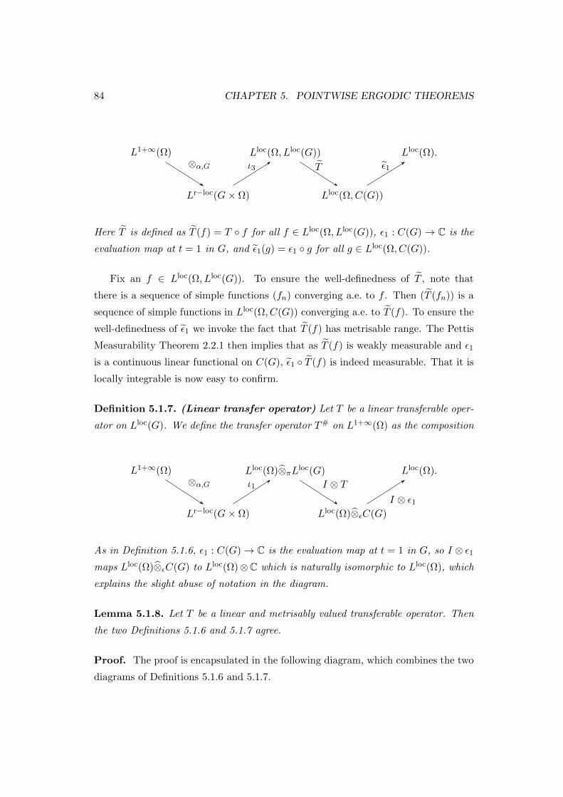
84 CHAPTER 5. POINTWISE ERGODIC THEOREMS
L1+∞(Ω)
Lr−loc(G× Ω)
Lloc(Ω, Lloc(G))
Lloc(Ω, C(G))
Lloc(Ω).⊗α,G ι3 T ε1
Here T is defined as T (f) = T f for all f ∈ Lloc(Ω, Lloc(G)), ε1 : C(G)→ C is the
evaluation map at t = 1 in G, and ε1(g) = ε1 g for all g ∈ Lloc(Ω, C(G)).
Fix an f ∈ Lloc(Ω, Lloc(G)). To ensure the well-definedness of T , note that
there is a sequence of simple functions (fn) converging a.e. to f . Then (T (fn)) is a
sequence of simple functions in Lloc(Ω, C(G)) converging a.e. to T (f). To ensure the
well-definedness of ε1 we invoke the fact that T (f) has metrisable range. The Pettis
Measurability Theorem 2.2.1 then implies that as T (f) is weakly measurable and ε1
is a continuous linear functional on C(G), ε1 T (f) is indeed measurable. That it is
locally integrable is now easy to confirm.
Definition 5.1.7. (Linear transfer operator) Let T be a linear transferable oper-
ator on Lloc(G). We define the transfer operator T# on L1+∞(Ω) as the composition
L1+∞(Ω)
Lr−loc(G× Ω)
Lloc(Ω)⊗πLloc(G)
Lloc(Ω)⊗εC(G)
Lloc(Ω).⊗α,G ι1 I ⊗ T
I ⊗ ε1
As in Definition 5.1.6, ε1 : C(G)→ C is the evaluation map at t = 1 in G, so I ⊗ ε1maps Lloc(Ω)⊗εC(G) to Lloc(Ω)⊗C which is naturally isomorphic to Lloc(Ω), which
explains the slight abuse of notation in the diagram.
Lemma 5.1.8. Let T be a linear and metrisably valued transferable operator. Then
the two Definitions 5.1.6 and 5.1.7 agree.
Proof. The proof is encapsulated in the following diagram, which combines the two
diagrams of Definitions 5.1.6 and 5.1.7.

5.2. SEMILOCALITY AND TRANSLATION INVARIANCE 85
Lr−loc(G× Ω)
Lloc(Ω, Lloc(G)) Lloc(Ω, C(G))
Lloc(Ω)
Lloc(Ω)⊗πLloc(G) Lloc(Ω)⊗εC(G)
ι3
T
ε1
ι1
I ⊗ T
I ⊗ ε1
Its commutativity can be easily checked for simple functions in Lr−loc(G × Ω),
and so by continuity of all the arrows, the commutativity of the diagram follows.
Now that the well-definedness of the Transfer Principle has been established and
it is clear what countability assumptions are used, let us give a simpler, working
definition. We emphasise that this working definition depends on the above analysis
for its correctness.
Remark 5.1.9. Let T be a sublinear transferable operator with metrisable range.
Starting with a function f ∈ L1+∞(Ω), define as before F (t, ω) := f(αt(ω)) and
F ′(t, ω) := (T (Fω))(t), where Fω is the cross section of F at ω ∈ Ω. Finally, we set
T#(f) := F ′(1, ω). Note that F ′ as defined above is in Lloc(Ω, C(G)).
Obviously, the steps followed in this Remark are exactly the steps used in Defini-
tion 5.1.6. As we will be working quite a bit with the functions F and F ′ given above,
there is another point that must be made about them. Firstly F is measurable on
G × Ω and indeed rectangular locally integrable as shown in Lemma 5.1.5. For F ′,
the situation is a little more tricky. By Lemma 2.3.5, F ′ is a well-defined measurable
function. However, it is not necessarily locally integrable or even rectangular locally
integrable. But when working out the maximal inequalities of Section 5.5, we shall
need only the Fubini result of equation (2.5).
Note that of course in the case where G is second countable, one could use Lemma
2.3.6 instead of Lemma 2.3.5 to prove the measurability of F ′.
5.2 The effect of semilocality and translation invariance
Let T be a transferable operator with metrisable range. We now describe some
approximation properties of T# that will be useful in the next section. We start by

86 CHAPTER 5. POINTWISE ERGODIC THEOREMS
extending some constructions that we have used earlier. Let K be any measurable
subset of G. As in equation (5.1), we can define the operator ⊗α,K on the set of
measurable functions on Ω by setting FK := ⊗α,K(f) := χK ⊗α f on G × Ω using
Definition 5.1.3. Hence
FK(t, ω) =
f(αt(ω)) if t ∈ K
0 if t /∈ K.(5.2)
In this notation, FG = F . We shall also use the notation F ′K = T (FK) where T is
as given in Definition 5.1.6. In particular, F ′ = F ′G. By Lemma 2.3.5, the functions
F ′K are measurable on G× Ω.
Lemma 5.2.1. Let T be a transferable operator with metrisable range and let U be
the open neighbourhood satisfying the conditions stated in Definition 5.1.2(2). Let K
and E be measurable subsets of G such that EU−1 ⊆ K. For any f ∈ L1+∞(Ω), and
almost all (t, ω) ∈ E × Ω, we have
|F ′(t, ω)| ≤ |F ′K(t, ω)|. (5.3)
Proof. First note that FKc = (χG − χK) ⊗α f = χG ⊗α f − χK ⊗α f = F − FK .Consequently,
|F ′| = |T (F )| = |T (F − FK + FK)|
≤ |T (FKc)|+ |T (FK)|
= |F ′Kc |+ |F ′K |.
By the semilocality of T , for almost every ω ∈ Ω, the measurable map t 7→ F ′Kc(t, ω)
has support in KcU . Because EU−1 ⊆ K, it follows that (KcU) ∩ E is empty since
a ∈ (KcU) ∩ E implies that there is a b ∈ U so that ab−1 ∈ Kc ∩ (EU−1), which is
impossible if EU−1 ⊆ K. Hence |F ′(t, ω)| ≤ |F ′K(t, ω)| for almost all ω ∈ Ω and all
t ∈ E.
Translation invariant operators, a class that includes all convolution operators, are
automatically equimeasurability-preserving, in a sense made precise by the following
Lemma.
5.3. AN EXAMPLE 87
Lemma 5.2.2. Let T be a transferable operator with metrisable range. For any
f ∈ L1+∞(Ω), all s, t ∈ G and almost all ω ∈ Ω,
F ′(t, αs(ω)) = F ′(ts, ω).
Moreover, for any t1, t2 ∈ G, the mappings ω 7→ F ′(t1, ω) and ω 7→ F ′(t2, ω) are
equimeasurable.
Proof. By definition of F , for µ-a.e. ω and any s, t ∈ G, we have
F (t, αs(ω)) = f αt(αs(ω)) = f αts(ω) = F (ts, ω).
Let τt : G → G be defined by τt(s) = ts for all s, t ∈ G as in Definition 5.1.2. By
definition of F ′ and the translation-invariance of T , we have
F ′(t, αs(ω)) = T F (t, αs(ω))
= T F (ts, ω)
= T τt F (s, ω)
= τt T F (s, ω)
= F ′(ts, ω).
Finally, let s = t−11 t2 and λ > 0. Then as F ′(t2, ω) = F ′(t1, αs(ω)), we see that
µ(ω : |F ′(t2, ω)| > λ) = µ(ω : |F ′(t1, αs(ω))| > λ)
= µ(α−1s (ω) : |F ′(t1, ω)| > λ)
= µ(ω : |F ′(t1, ω)| > λ),
proving the equimeasurability of the maps ω 7→ |F ′(t1, ω)| and ω 7→ |F ′(t2, ω)|.
The last two lemmas will both be needed in the proof of Lemma 5.5.1.
5.3 An example
One of the main sources of transferable operators in applications is convolution op-
erators. The straightforward construction of ergodic averaging operators from con-
volution operators demonstrates the utility and ubiquity of the transfer operator
construction.

88 CHAPTER 5. POINTWISE ERGODIC THEOREMS
Suppose that O is a measure-preserving automorphism on the measure space
(Ω, µ). It induces an action α of Z on Ω via α(n) := On. If S is a finite subset of
Z, let TS be the convolution operator defined on the space of all locally integrable
functions f on Z by
TS(f) :=1
|S|χ−S ∗ f,
where of course χ−S is the characteristic function of −S. Bearing in mind that
the set of locally integrable functions on Z is precisely the set of all complex-valued
functions, we see that TS is well-defined, linear and takes its values in C(Z), which
is metrisable. From the properties of convolution, it is clearly semi-local. Indeed, if
N = max|s| : s ∈ S and f is a function with support in [−M,M ], then TS(f) will
have support in [−M −N,M +N ].
Let us now determine the transfer operator T#S . Let f ∈ L1+∞(Ω). With the
help of Definition 5.1.6 and Lemma 2.3.5, we compute:
TS(F (t, ω)) = TS(f(αt(ω)))
=1
|S|∑s∈S
f(αt+s(ω)).
Hence
T#S (f)(ω) = ε0 TS(F )(ω) =
1
|S|∑s∈S
f(αs(ω)),
which is a locally integrable function on Ω. (Note that we write ε0 above because 0
is the identity element of Z).
5.4 Kolmogorov’s inequality for r.i. BFSs
The next two Sections are devoted to calculating the type of the transfer operator
T# from information on the type of T .
The following theorem will be useful in determining the weak type of an operator.
It is an extension of Kolmogorov’s criterion as found in [12].
Theorem 5.4.1. Let (Ω, µ) be a measure space and let T be an operator on some
class of measurable functions on Ω that maps into the set of measurable functions on
Ω. Suppose that T is of weak type (X,Y ) for r.i. BFSs X and Y and has norm c.
Let ϕ be the fundamental function of the space Y . If 0 < σ < 1 and A is any subset

5.4. KOLMOGOROV’S INEQUALITY FOR R.I. BFSS 89
of Ω of finite measure, then for any f ∈ X we have∫A|Tf |σ dµ(x) ≤ cσ
1− σ[ϕ∗(|A|)
]σ|A|1−σ‖f‖σX . (5.4)
Conversely, if T satisfies this inequality for some c and 0 < σ < 1, and for each
f ∈ X and each A ⊂ Ω with finite measure, then T is of weak type (X,Y ).
Proof. Suppose 0 < σ < 1. As t 7→ ϕ(t)/t is nondecreasing, if s ≤ t, we have the
implications
ϕ(s)
s≥ ϕ(t)
t=⇒ ϕ(t)
ϕ(s)≤ t
s=⇒ ϕσ(t)
ϕσ(s)≤( ts
)σ=⇒ s
tϕσ(t) ≤
( ts
)σ−1ϕσ(s).
Note that χ[1,∞)(t/s) = χ(0,t](s) for all s, t ∈ R+. On the multiplicative group of
the positive reals, we now compute, using the convolution of the functions [(Tf)σ]∗(x)ϕσ(x)
and xσ−1χ[1,∞)(x) at t ∈ R:
ϕσ(t)
t
∫ t
0[(Tf)σ]∗(s)ds ≤
∫ t
0[(Tf)σ]∗(s)ϕσ(s)
( ts
)σ−1ds
s
=
∫ ∞0
[(Tf)σ]∗(s)ϕσ(s)( ts
)σ−1χ(0,t](s)
ds
s
=
∫ ∞0
[(Tf)σ]∗(s)ϕσ(s)( ts
)σ−1χ[1,∞)(t/s)
ds
s
= [(Tf)σ]∗(x)ϕσ(x) ∗ xσ−1χ[1,∞)(x)∣∣t.
With this in hand, we exploit the inequality
‖[(Tf)σ]∗(x)ϕσ(x) ∗ xσ−1χ[1,∞)(x)‖∞ ≤ ‖[(Tf)σ]∗(x)ϕσ(x)‖∞‖xσ−1χ[1,∞)(x)‖1.
As ‖xσ−1χ[1,∞)(x)‖1 =
∫ ∞1
sσ−2ds =1
σ − 1sσ−1
∣∣∞1
=1
1− σ, we have
supt>0
ϕσ(t)
t
∫ t
0[(Tf)σ]∗(s)ds ≤ 1
1− σsupt>0
[(Tf)σ]∗(t)ϕσ(t) =1
1− σ[
supt>0
(Tf)∗(t)ϕ(t)]σ.
Here we used the fact that (|f |σ)∗ = (|f |∗)σ for all 0 < σ < ∞ (see Prop 2.1.7
p41 of [4]). We thus have the following inequality.
ϕσ(t)
t
∫ t
0[(Tf)σ]∗(s)ds ≤ 1
1− σ‖Tf‖σM∗(Y )
≤ cσ
1− σ‖f‖σX ,

90 CHAPTER 5. POINTWISE ERGODIC THEOREMS
by our hypothesis. It is obvious that
∫A|Tf |σ dµ ≤
∫ |A|0
[(Tf)σ]∗(s)ds, and so we
obtain ∫A|Tf |σ dµ ≤ cσ
1− σ|A|
ϕσ(|A|)‖f‖σX
=cσ
1− σ[ϕ∗(|A|)
]σ|A|1−σ‖f‖σX .To get the last equality, we used the identity ϕ(|A|)ϕ∗(|A|) = |A|.
To prove the converse, suppose that T satisfies (5.4) for some 0 < σ < 1 and fix
λ > 0. Consider a set K ⊂ ω : |Tf(ω)| > λ of finite measure. By hypothesis,
|K| ≤∫K
|Tf |σ
λσdµ ≤ 1
λσcσ
1− σ[ϕ∗(|K|)]σ|K|1−σ‖f‖σX .
Consequently, the following computations are valid:
|K|σ
ϕ∗(|K|)σ≤ 1
λσcσ
1− σ‖f‖σX ;
ϕ(|K|) ≤ 1
λ
c
(1− σ)1/σ‖f‖X ;
λϕ(m(|Tf |, λ)) ≤ c
(1− σ)1/σ‖f‖X ;
‖Tf‖M∗(Y ) ≤c
(1− σ)1/σ‖f‖X ;
where in the last line we used the identity ‖Tf‖M∗(Y ) = supλ>0 λϕY (m(|Tf |, λ)) of
Lemma 3.1.3. This proves the converse.
Note that the proof remains correct even if ‖ · ‖X is a seminorm.
Although we shall not need the concept here, this theorem, and especially the
inequality (5.4), suggest a further refinement of the idea of weak-type operators.
Definition 5.4.2. Let T be an operator on a BFS X on the measure space (Ω, µ)
taking values in the space of measurable functions on (Ω, µ). Let A be a class of
measurable µ-finite subsets of Ω. We say that T is of A-weak type (X,Y ) if∫A|Tf |σ dµ(x) ≤ cσ
1− σ[φ∗|A|
]σ|A|1−σ‖f‖σΛ(ψ)
holds for all A ∈ A.
In particular if Ω is a product space and A is the class of all µ-finite measurable
rectangles, we say that T is of rectangular weak-type (X,Y ).

5.5. THE WEAK TYPE OF THE TRANSFERRED OPERATOR 91
5.5 Computation of the weak type of the transferred
operator
In the rest of the paper, we shall work with dynamical systems (G,Ω, µ, α) as given in
Definition 5.1.1, where (Ω, µ) is a countably generated σ-finite and resonant measure
space and G is a σ-finite locally compact group.
We can now state and prove results on the weak type of the transfer operator,
which form one of the main themes of this work. The next lemma is the key technical
ingredient. It is in this Lemma that the semilocality and equimeasurability-preserving
properties of the transferable operator are used.
Lemma 5.5.1. Let X,Y be r.i. BFSs over G with fundamental functions ϕX and
ϕY respectively and let T be a transferable operator of weak type (X,Y ) with metris-
able range. Let U be the open neighbourhood satisfying the conditions in Definition
5.1.2(2). Then for any subset A ⊂ Ω of finite measure, and 0 < σ < 1, there is a
compact neighbourhood K of the identity such that
1
|A|
∫A|T#f |σ(ω)dµ ≤ 2cσ
1− σ[ϕY (|K|)]−σ
(1
|A|
∫A‖(F
KU−1)ω‖X dµ
)σ,
where for each ω ∈ Ω the cross section (FKU−1)ω is the measurable function defined
on G by t 7→ FKU−1(t, ω).
Proof. By the Fubini-type Lemma 2.3.5 and Lemma 5.2.1, which we employ by iden-
tifying E with K and K with KU−1, we have:∫K
∫A|F ′(t, ω)|σ dµdt =
∫A
∫K|F ′(t, ω)|σ dtdµ
≤∫A
∫K|F ′KU−1(t, ω)|σ dtdµ.
As T is of weak type (X,Y ), using Kolmogorov’s criterion (5.4) we have that∫K|F ′KU−1(t, ω)|σdt ≤ cσ
1− σ[ϕ∗Y (|K|)]σ|K|1−σ‖(F
KU−1)ω‖σX .
From Jensen’s inequality and the identity ϕ∗Y (t)ϕY (t) = t,∫K
∫A|F ′(t, ω)|σ dµdt ≤ cσ
1− σ[ϕ∗Y (|K|)]σ|K|1−σ
∫A‖(F
KU−1)ω‖σX dµ
≤ cσ
1− σ[ϕY (|K|)]−σ|K||A|1−σ
(∫A‖(F
KU−1)ω‖X dµ
)σ.

92 CHAPTER 5. POINTWISE ERGODIC THEOREMS
We rewrite this as
1
|K|
∫K
[1
|A|
∫A|F ′(t, ω)|σ dµ
]dt ≤ cσ
1− σ[ϕY (|K|)]−σ
(1
|A|
∫A‖(F
KU−1)ω‖X dµ
)σ.
As
t 7→ 1
|A|
∫A|F ′(t, ω)|σdµ
is continuous, and as |F ′(1, ω)| = |T#f |(ω) by definition, from the Lebesgue differ-
entiation Theorem we obtain
1
|A|
∫A|T#f |σ(ω)dµ = lim
K→1
1
|K|
∫K
[1
|A|
∫A|F ′(t, ω)|σ dµ
]dt.
Hence for some K small enough,
1
|A|
∫A|T#f |σ(ω)dµ ≤ 2
|K|
∫K
[1
|A|
∫A|F ′(t, ω)|σ dµ
]dt
≤ 2cσ
1− σ[ϕY (|K|)]−σ
(1
|A|
∫A‖(F
KU−1)ω‖X dµ
)σ.
Corollary 5.5.2. Let (Ω, µ,G, α) be a dynamical system with (Ω, µ) countably gen-
erated and resonant and let T be a transferable operator of weak type (X,Y ) and
suppose that ΦA and ΦB are Young’s functions with respective associated fundamen-
tal functions ϕA and ϕB satisfying
θϕA(st) ≥ ϕX(s)ϕB(t)
for some θ > 0 and all s, t > 0.
1) If X is an Orlicz space and limt→0 ϕ∗X(t) = 0, then T# is of weak type (L(ΦA), ϕB).
2) If X is an M - space then T# is of weak type (M(ϕA), ϕB).
3) If X is a Λ-space and limt→0 ϕ∗X(t) = 0, then T# is of weak type (Λ(ϕA), ϕB).
Proof. We prove part 3). Let A ⊂ Ω have finite measure and let U be the open
neighbourhood guaranteed by Definition 5.1.2(2). Then for any 0 < σ < 1, by
Lemma 5.5.1, there is a compact neighbourhood of the identity K ⊂ G such that
1
|A|
∫A|T#f |σ(ω)dµ ≤ 2cσ
1− σ[ϕY (|K|)]−σ
(1
|A|
∫A‖(FKU−1)ω‖Λ(X) dµ
)σ.
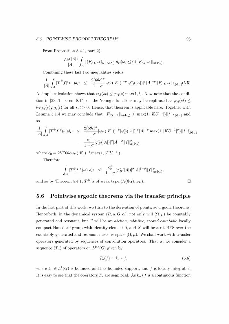
5.6. POINTWISE ERGODIC THEOREMS 93
From Proposition 3.4.1, part 2),
ϕB(|A|)|A|
∫A‖(FKU−1)ω‖Λ(X) dµ(ω) ≤ 6θ‖FKU−1‖Λ(ΦA).
Combining these last two inequalities yields
1
|A|
∫A|T#f |σ(ω)dµ ≤ 2(6θc)σ
1− σ[ϕY (|K|)]−σ[ϕ∗B(|A|)]σ|A|−σ‖FKU−1‖σΛ(ΦA).(5.5)
A simple calculation shows that ϕA(st) ≤ ϕA(s) max(1, t). Now note that the condi-
tion in [33, Theorem 8.15] on the Young’s functions may be rephrased as ϕA(st) ≤θϕA0(s)ϕB0(t) for all s, t > 0. Hence, that theorem is applicable here. Together with
Lemma 5.1.4 we may conclude that ‖FKU−1‖Λ(ΦA) ≤ max(1, |KU−1|)‖f‖Λ(ΦA) and
so
1
|A|
∫A|T#f |σ(ω)dµ ≤ 2(6θc)σ
1− σ[ϕY (|K|)]−σ[ϕ∗B(|A|)]σ|A|−σ max(1, |KU−1|σ)‖f‖σΛ(ΦA)
=cσ0
1− σ[ϕ∗B(|A|)]σ|A|−σ‖f‖σΛ(ΦA)
where c0 = 21/σ6θcϕY (|K|)−1 max(1, |KU−1|).Therefore ∫
A|T#f |σ(ω) dµ ≤ cσ0
1− σ[ϕ∗B(|A|)]σ|A|1−σ‖f‖σΛ(ΦA),
and so by Theorem 5.4.1, T# is of weak type (Λ(ΦA), ϕB).
5.6 Pointwise ergodic theorems via the transfer principle
In the last part of this work, we turn to the derivation of pointwise ergodic theorems.
Henceforth, in the dynamical system (Ω, µ,G, α), not only will (Ω, µ) be countably
generated and resonant, but G will be an abelian, additive, second countable locally
compact Hausdorff group with identity element 0, and X will be a r.i. BFS over the
countably generated and resonant measure space (Ω, µ). We shall work with transfer
operators generated by sequences of convolution operators. That is, we consider a
sequence (Tn) of operators on Lloc(G) given by
Tn(f) = kn ∗ f, (5.6)
where kn ∈ L1(G) is bounded and has bounded support, and f is locally integrable.
It is easy to see that the operators Tn are semilocal. As kn∗f is a continuous function

94 CHAPTER 5. POINTWISE ERGODIC THEOREMS
and C(G) is metrisable, we see that these operators satisfy the definition of linear
transferable operators with metrisable range given in Definition 5.1.2. We also define
Tf := supn |Tn(f)|. Using the Transfer Principle and given information about the
functions kn and the space X, we show that the transferred operators T#n satisfy a
pointwise convergence theorem: that is, T#n f(ω) converges a.e. for all f ∈ X as n
tends to infinity.
To achieve this goal, our strategy is the following three step programme.
1. Given the weak type of the operator T , find the weak type of T#.
2. In the domain of T# computed in step (1), identify a dense subset D for which
the pointwise convergence of (T#n f) can be verified for all f ∈ D.
3. Use an appropriate version of Banach’s Principle to extend the a.e. convergence
of step (2) to the whole domain of T#.
To do step (1), we shall use results such as the following:
Proposition 5.6.1. Let (Tn) be a sequence of operators given by (5.6). Suppose
there are Young’s functions ΦA, ΦB,ΦC ,ΦD and ΦE with associated fundamental
functions ϕA, . . . , ϕE satisfying
ϕC(t)ϕ∗B(s) ≤ θ1ϕA(st)
ϕA(st) ≤ θ2ϕD(s)ϕE(t)
for all s, t > 0.
Suppose further that there are measurable functions `0 and `1 on G such that
sup |kn(s−1)| = `0(s)`1(s), `0 ∈ L(ΦB) and `1 ∈ L(ΦE). Then the operator T#
defined by T#f(ω) = supn∈N |T#n f |(ω) is a sublinear operator mapping L(ΦD) into
L(ΦC).
Proof. For each N ∈ N, let SNf(ω) := max1≤n≤N |T#n f |(ω). By [33, Theorem 8.18],
‖SNf‖L(ΦC) ≤ ‖ max1≤n≤N
∣∣ ∫Gkn(s−1)f(αs(ω)) ds
∣∣‖L(ΦC)
≤ ‖∫G
max1≤n≤N
|kn(s−1)||f(αs(ω))|ds‖L(ΦC)
≤ θ‖`1‖L(ΦB)‖`0 ⊗α f‖L(ΦA)
= θ1‖`1‖L(ΦB)‖`0 ⊗ f‖L(ΦA)(by Lemma 5.1.4)
≤ θ1θ2`1‖L(ΦB)‖`0‖L(ΦE)‖f‖L(ΦD)

5.6. POINTWISE ERGODIC THEOREMS 95
where the final inequality follows from [33, Theorem 8.15].
For step (3), we prove the following variation on the theme of [4, Corollary 4.5.8]
and [20, Theorem 1.1.1], which provides the final link between maximal inequalities
and pointwise ergodic theorems.
The following result in essence amounts to an extension of that part of the Banach
principle cycle of ideas that we need to complete our program.
Proposition 5.6.2. Let X and Y be r.i. BFSs over a measure space (Ω, µ). Let
(Tn) be a sequence of linear operators on X and define the maximal operator T by
T (f) = supn |Tn(f)|. If
1. there is a dense subset D ⊆ X such that for all f ∈ D, (Tn(f)(ω)) converges
for µ-a.e. ω ∈ Ω,
2. T is of weak-type (X,Y ),
then (Tn(f)(ω)) converges for µ-a.e. ω ∈ Ω and all f ∈ X.
Proof. Define the oscillation Of of f ∈ X as follows. For any ω ∈ Ω set
Of (ω) = lim supn,m→∞
|Tn(f)(ω)− Tm(f)(ω)|.
Clearly the linearity of the operators Tn implies that Of (ω) ≤ Og(ω) +Of−g(ω).
For any g ∈ D, (Tng) converges µ-a.e. and thus Og = 0 µ-a.e.
Pick an f ∈ X. Now for any η > 0, there is a g ∈ D such that ‖f − g‖X < η and
µ(ω : Of (ω) > δ) ≤ µ(ω : Of−g(ω) > δ).
Furthermore, by the definition of the oscillation, Of (ω) ≤ 2T (f)(ω) a.e. Similarly
for Of−g. Hence
µ(ω : Of (ω) > δ) ≤ µ(ω : 2T (f − g)(ω) > δ)
= m(2T (f − g), δ).
As T is of weak-type (X,Y ), ‖2T (f−g)‖M∗(Y ) ≤ 2β‖f−g‖X < 2βη where β depends
only on T . Rewriting this using Lemma 3.1.3,
sups>0
sϕY (m(2T (f − g), s)) ≤ 2βη,

96 CHAPTER 5. POINTWISE ERGODIC THEOREMS
In particular, δϕY (m(2T (f − g), δ)) ≤ 2βη. Therefore
ϕY (µ(ω : Of (ω) > δ)) ≤ 2βη
δ.
As η is arbitrary, ϕY (µ(ω : Of (ω) > δ)) = 0. Because a fundamental function is
0 only at the origin, µ(ω : Of (ω) > δ) = 0. Because δ is arbitrary, Of = 0 µ-a.e.
which implies that (Tnf) does indeed converge µ-a.e.
The fundamental result towards completing step (2) of the three-step programme
is given in Proposition 5.6.4. From this, many interesting pointwise ergodic theo-
rems can be deduced, given further information on the nature of X. We start by
constructing subsets D of X for whose elements a.e. convergence is easy to check. To
this end, for any f ∈ L1(G) and x ∈ X, we define
αf (x) =
∫Gαt(x)f(t) dt, (5.7)
where the integral is a Bochner integral. Because the action of G on (Ω, µ) is measure-
preserving, on any r.i. BFS the automorphism αt is an isometry and so αf (x) ∈ Xtoo.
Note that the above equation actually gives a bounded bilinear mapping from
L1(G)×X into X, given by (f, x) 7→ αf (x).
Definition 5.6.3. Let Y be a set of measurable functions on (Ω, µ) and L ⊆ L1(G).
Define
DX(Y,L) = αf (x) : f ∈ L, x ∈ X ∩ Y ,
which is a subset of X. In particular, if F0 consists of those integrable functions on
G with vanishing integral, we shall simply write DX for DX(L∞(Ω),F0).
Proposition 5.6.4. Let (Ω, µ,G, α) be a dynamical system and (Tn) a sequence of
convolution operators given by (5.6). Suppose that (kn ∗ φ) converges weakly in L1
for all φ ∈ L1(G) with vanishing integral.
Then given a r.i. BFS X, the sequence (T#n f) converges a.e. for every f ∈ DX .
Proof. We begin by describing T#n explicitly, using the construction of Remark
5.1.9. Let f ∈ X. For almost every ω ∈ Ω, the function t 7→ f(αtω) is locally
integrable by Lemma 5.1.5 and so by definition of Tn we have
Tnf(αtω) =
∫Gkn(−s)f(αs−tω) ds.

5.6. POINTWISE ERGODIC THEOREMS 97
Because we have assumed that kn is bounded and has bounded support, the integral
converges for any locally integrable f , and in particular for any f ∈ X. Setting t = 0,
we obtain
T#n f(ω) =
∫Gkn(−s)f(αsω) ds. (5.8)
We prove that for any f ∈ DX , the sequence (T#n (f)) converges a.e. By definition
of DX , there exists a g ∈ L∞(Ω) ∩ X and ψ ∈ L1(G) with vanishing integral, such
that f = αψ(g). We compute:
T#n f(ω) =
∫Gkn(−t)f(αtω) dt
=
∫Gkn(−t)
∫Gg(αt+sω)ψ(s) ds dt
=
∫Gg(αtω)
∫Gkn(s− t)ψ(s) ds dt.
As the inner integrals converge weakly in L1(G), and bearing in mind that g ∈L∞(Ω), we have proved that (T#
n (f)) converges a.e.
In the light of Propositions 5.6.2 and 5.6.4, to complete the three-step programme
and prove pointwise ergodic theorems, we indicate situations where we can use the
space DX to construct dense subsets of X.
First, we must establish a lemma that will allow us to construct invariant subsets
for a given dynamical system. Recall from [4, Definition 1.3.1] that a function norm
on a r.i. BFS X over a measure space (Ω, µ) is absolutely continuous if for every nested
decreasing sequence (An) of measurable subsets of Ω such that χAn → 0 µ-a.e. as
n→∞, and any f ∈ X, we have ‖fχAn‖X → 0 as n→∞.
Lemma 5.6.5. Let X be a r.i. BFS over a σ-finite measure space (Ω, µ), f be a
function in X and λ > 0. If X has absolutely continuous norm then m(f, λ) <∞.
In particular, the conclusion holds if X is reflexive.
Proof. Suppose to the contrary that there is a λ > 0 and f ∈ X such that m(f, λ) =
∞. Set Λ = ω : |f(ω)| > λ. As Ω is σ-finite there is an increasing sequence of
finite-measure sets Kn such that ∪Kn = Λ. Set Cn = Λ\Kn. Clearly µ(Cn) =∞.
Because λχΛ ≤ |f |, λχΛ, and hence χΛ itself, are in X. So are the characteristic
functions χCn for all n.
98 CHAPTER 5. POINTWISE ERGODIC THEOREMS
But as Cn ↓ ∅, the hypothesis that X has absolutely continuous norm implies
that
limn→∞
‖χCn‖X = limn→∞
‖χΛχCn‖X = 0. (5.9)
However, it is easy to compute that χ∗∗Cn(t) = 1 for all t > 0 and so
ϕX(1) ≤ supt>0
χ∗∗Cn(t)ϕX(t) = ‖χCn‖M(X) ≤ ‖χCn‖X .
This contradicts (5.9) and so we conclude that our hypothesis m(f, λ) = ∞ is
false.
In the case that X is reflexive, note that by [4, Corollary 1.4.4], its norm is
absolutely continuous.
Theorem 5.6.6. In the setup of Proposition 5.6.4, suppose that X is reflexive and
that T# has weak type (X,Y ). Then (T#n f) converges a.e. for every f ∈ X.
Proof. By hypothesis, T# is of weak type (X,Y ). The plan of the proof is to
execute steps (2) and (3) of the three step programme: identify a dense subset D of
X and use Proposition 5.6.4 to show the a.e. convergence of the sequence (T#n f) for
f ∈ D, prove that D is dense in X, and then finally invoke Proposition 5.6.2 to show
that (T#n f) converges a.e. for all f ∈ X.
We consider the set D = DX+F , where F is the subspace of all fixed points of the
action α in X. We have already seen in Proposition 5.6.4 that (T#n (f)) converges a.e.
for all f ∈ DX . Similarly, if g ∈ F , it is easy to see from (5.8) that as t 7→ g(αtω) =
g(ω) for almost every ω ∈ Ω, T#n g(ω) = g(ω)
∫Gkn(−s) ds a.e. From the assumption
that the sequence( ∫
G kn(s) ds)
converges, it follows that (T#n g(ω)
)converges a.e.
for all g ∈ F . Therefore (T#n (f)) converges a.e. for all f ∈ D.
The next task is to demonstrate that D is dense in X. By [4, Corollary 1.4.3],
the associate space X ′ is also the dual of X. Let ` ∈ X ′ be orthogonal to D. We
must show that ` = 0 µ-a.e. We may assume that ` is real-valued, because if ` is
orthogonal to D, so is `.

5.6. POINTWISE ERGODIC THEOREMS 99
For any f = αψ(g) ∈ DX ⊆ D we have
0 =
∫Ω`(ω)f(ω) dµ(ω) =
∫Ω`(ω)
∫Gg(αtω)ψ(t) dtdµ(ω)
=
∫Ω
∫G`(ω)g(αtω)ψ(t) dtdµ(ω)
=
∫Ω
∫G`(α−tω)g(ω)ψ(t) dtdµ(ω)
=
∫Ωg(ω)
∫Gψ(t)`(α−tω) dtdµ(ω).
The absolute continuity of the norm of X and [4, Theorem 1.3.11] imply that
Xb = X. Hence L∞(Ω) ∩ X is dense in X. By definition of DX , g is an arbitrary
element of L∞(Ω) ∩X and therefore∫Gψ(t)`(α−tω) dt = 0.
Now we use some basic ideas from spectral synthesis, as presented in [17, Section
4.6] and [41, Section 7.8]. We write
F⊥0 =ξ ∈ L∞(G) :
∫Gψ(t)ξ(t) dt = 0 for all ψ ∈ F0
.
Clearly F⊥0 is a translation-invariant subspace of L∞(G) and F0 is a closed ideal in
L1(G). Furthermore,
ν(F0) = ξ ∈ G : f(ξ) = 0 for all f ∈ F0 = 0.
To see this, first note that for any f ∈ L1(G),∫G f(t) dt = f(0), so the fact that
each f ∈ F0 has vanishing integral means that 0 ∈ ν(F0).
Now suppose there was a ξ ∈ G, ξ 6= 0, such that ξ ∈ ν(F0). Then f ∈ F0 implies
that f(ξ) = 0. In other words, ker ξ ⊇ F0 =ker 0.
But as 0 and ξ are linear functionals, this means that ker 0 =ker ξ, and that there
is a non zero λ ∈ C such that 0 = λξ.
Now take any two f, g ∈ L1(G) such that 0(f), 0(g) 6= 0. Then
λξ(f ∗ g) = 0(f ∗ g) = 0(f)0(g) = λ2ξ(f ∗ g),
so λ = 1 . Hence 0 = ξ and ξ = 0, a contradiction.
Recall that for any translation-invariant subspace M ⊆ L∞(G), the spectrum
σ(M) is the set of all continuous characters in M:
σ(M) =M∩ G.
100 CHAPTER 5. POINTWISE ERGODIC THEOREMS
By [17, Proposition 4.73], σ(F⊥0 ) = ν(F0) = 0. By [17, Proposition 4.75 b)], F⊥0 is
the linear span of the constant character and so consists of the constant functions.
From this analysis we conclude that t 7→ `(α−tω) ∈ F⊥0 is a constant for a.e.
ω ∈ Ω. We can write this fact as αt(`) = ` for all t ∈ G.
To complete the proof that D is dense in X, we must show that ` = 0 a.e. Fix
a λ > 0 and define Λ = ω : `(ω) > λ. By the reflexivity of X ′ = X∗ and Lemma
5.6.5, |Λ| ≤ m(f, λ) < ∞. This set is invariant under α (because αt(`) = ` for all
t ∈ G) and of course χΛ ∈ X. So a fortiori χΛ ∈ F . As ` is orthogonal to F as well,
we have
0 =
∫ΩχΛ` dµ ≥ λ|Λ|,
which implies that |Λ| = 0. As this holds for all λ > 0, we have proved that ` ≤ 0
µ-a.e. But now the same argument applied to the sets Λ′ = ω : `(ω) < −λ, where
λ is an arbitrary positive number, shows that |Λ′| = 0 for all λ > 0, and so ` = 0
µ-a.e.
Thus we have shown that any function in X ′ orthogonal to D must be the zero
function, proving the density of D in X. We have already proved that (T#n (f))
converges a.e. for all f ∈ D. Applying Proposition 5.6.2, the Theorem is proved.
If we have more information about the action α, we can relax the conditions on
the space X. In the next corollary, given additional assumptions about the group
action, we shall not need the reflexivity of X.
Corollary 5.6.7. In the setup of Theorem 5.6.6, if X has absolutely continuous
norm and the fixed point space F is finite dimensional, then (T#n f) converges a.e. for
every f ∈ X.
In particular, the result holds if the dynamical system is ergodic.
Proof. As F is finite dimensional, we can find a finite number of mutually disjoint
subsets AnNn=1 such that F is spanned by χAn for 1 ≤ n ≤ N . Indeed if f ∈ F ,
then for every λ > 0, if we set Eλ = ω : |f(ω)| > λ, then χEλ ∈ F . As F is finite
dimensional, there can only be a finite number of different sets Eλ, and so f is a
linear combination of a finite number of characteristic functions, making f a simple
function. Hence F is spanned by a collection of simple functions. As F is finite
dimensional, such a collection must be finite.
By [4, Corollary 1.4.3], X ′ = X∗. Reasoning as in Theorem 5.6.6, we consider
the set D = DX + F , where F is the subspace of all fixed points of the action α in

5.7. NOTES AND REMARKS 101
X and let ` ∈ X ′ orthogonal to D. To prove the density of D in X, we must again
show that ` = 0 µ-a.e.
Firstly, as shown in the proof of Theorem 5.6.6, ` is invariant under the action
α. Hence for any λ > 0, ω : |`(ω)| > λ is an invariant subset of Ω. This implies
that ω : |`(ω)| > λ ∩ An is invariant and is either empty or equal to An. Hence
ω : |`(ω)| > λ either equals the empty set, An, or Acn. From this we conclude that `
is a (possibly trivial) linear combination of the characteristic functions χAn and χAcn
for 1 ≤ n ≤ N . Note that as χAcn ∈ F , it is a linear combination of the functions
χAnNi=1, so ` is really just a linear combination of the functions χAn .
As ` is orthogonal to F , this implies that ` = 0 a.e. Hence D is dense in X.
Applying Proposition 5.6.2, the Corollary is proved.
It is easy to prove that the action of G on (Ω, µ) is ergodic if and only if the only
invariant function is the characteristic function χΩ. In this case, F has dimension one
if Ω has finite measure, for then χΩ ∈ F , and F = 0 if Ω has infinite measure. This is
because if there was a non-zero f ∈ F , then as we have seen above, ω : |f(ω)| > λ is
an invariant subset of Ω for each λ > 0, contradicting the ergodicity of the action.
Finally, let us mention another way to obtain a dense subset of a r.i. BFSs on
which the pointwise convergence of the ergodic averages can readily be checked.
Corollary 5.6.8. In the setup of Theorem 5.6.6, if T# is also of weak type (E,Z)
for r.i. BFSs E and Z where E is reflexive and X ∩ E is dense in X, then (T#n f)
converges a.e. for every f ∈ X.
Proof. By Theorem 5.6.6, (T#n f) converges a.e. for all f ∈ Y . Hence we have a
dense subset of X, namely X ∩Y , on which the ergodic averages converge pointwise.
Applying Proposition 5.6.2 finishes the proof.
If for example X = L1(Ω) and Y = Z = Lp(Ω) for some 1 < p <∞, this Corollary
is applicable. A special case of this setup in given in [8, Theorem 3].
5.7 Notes and Remarks
Proposition 5.6.1 is due to Prof L. Labuschagne. He also corrected an earlier state-
ment in Proposition 3.4.1 and is also responsible for the current proof of part (3)
of Theorem 3.4.2, which is a lot shorter than the one originally offered. He and an

102 CHAPTER 5. POINTWISE ERGODIC THEOREMS
external examiner spotted an error in an earlier draft of Section 5.5 and was instru-
mental in finding a fix to the problem. These are just a few instances of his influence
which can be felt on every page of this work.
With three exceptions, all the results proved in this thesis are original (to the
author’s knowledge). One exception is the duly attributed first part of Lemma 3.3.6.
Nevertheless, it has a novel proof. The others are Lemmas 2.2.2 and 3.1.1, which we
included for completeness: many quote the results, though without proof.
Let us make a few remarks on the development of the ideas used in the pointwise
ergodic theory.
The author’s original intention was to follow Calderon’s lead in [8] and prove his
Theorem 2 for more general r.i. BFSs and locally compact abelian groups. Follow-
ing Calderon’s proof strategy closely, the author could only prove Corollary 5.5.2,
in a restricted sense: the measure space (Ω, µ) had to have finite measure and the
fundamental function had to be submultiplicative (i.e. essentially satisfy the ∆′ con-
dition. The breakthrough occurred in two stages: first was the generalisation of
Kolmogorov’s inequality 5.4.1, from its classical statement in [12]. A different proof
strategy also had to be found.
The power of Kolmogorov’s inequality is that it allows the determination of the
weak type of a operator to be related to an integral over a finitely measurable subset
- a localisation if you will. However, one must then estimate the integral of a func-
tion whose value is the norm of a cross section. This is why Proposition 3.4.1 was
developed. Note that it is to apply this result that the most stringent condition on
(Ω, µ) has to be imposed: that it be a countably generated measure space.

Bibliography
[1] W. Arveson. On groups of automorphisms of operator algebras. Journal of
Functional Analysis, 15:217–243, 1974.
[2] M. Bedford, T. Keane and C. Series, editors. Ergodic theory, symbolic dynamics,
and hyperbolic spaces. Oxford Science Publications. The Clarendon Press Oxford
University Press, New York, 1991.
[3] A. Bellow. Transference principles in ergodic theory. In Harmonic analysis and
partial differential equations (Chicago, IL, 1996), Chicago Lectures in Mathe-
matics, pages 27–39. Univ. Chicago Press, Chicago, IL, 1999.
[4] C. Bennett and R. Sharpley. Interpolation of operators, volume 129 of Pure and
Applied Mathematics. Academic Press Inc., Boston, MA, 1988.
[5] J. Bourgain. On the maximal ergodic theorem for certain subsets of the integers.
Israel Journal of Mathematics, 61(1):39–72, 1988.
[6] J. Bourgain. Pointwise ergodic theorems for arithmetic sets. Institut des Hautes
Etudes Scientifiques. Publications Mathematiques, (69):5–45, 1989. With an
appendix by the author, Harry Furstenberg, Yitzhak Katznelson and Donald S.
Ornstein.
[7] Z. Buczolich and R. D. Mauldin. Divergent square averages. Annals of Mathe-
matics. Second Series, 171(3):1479–1530, 2010.
[8] A.-P. Calderon. Ergodic theory and translation-invariant operators. Proceedings
of the National Academy of Sciences of the United States of America, 59:349–
353, 1968.
103
104 BIBLIOGRAPHY
[9] R. R. Coifman and G. Weiss. Transference methods in analysis. American Math-
ematical Society, Providence, R.I., 1976. Conference Board of the Mathematical
Sciences Regional Conference Series in Mathematics, No. 31.
[10] R. J. de Beer. Tauberian theorems and spectral theory in topological vector
spaces. Glasgow Mathematical Journal, published online Feb 2013, to appear.
[11] R. J. de Beer and L. E. Labuschagne. Maximal ergodic inequalities for Banach
function spaces. available at arXiv:1309.0125v1 [math.DS].
[12] M. de Guzman. Real variable methods in Fourier analysis, volume 46 of North-
Holland Mathematics Studies. North-Holland Publishing Co., Amsterdam, 1981.
Notas de Matematica, 75.
[13] J. Diestel. Sequences and series in Banach spaces, volume 92 of Graduate Texts
in Mathematics. Springer-Verlag, New York, 1984.
[14] J. Diestel and J. J. Uhl, Jr. Vector measures. American Mathematical Society,
Providence, R.I., 1977.
[15] N. Dunford and J. T. Schwartz. Linear operators. Part I. Wiley Classics Library.
John Wiley & Sons Inc., New York, 1988.
[16] C. Finet and P. Wantiez. Transfer principles and ergodic theory in Orlicz spaces.
Note di Matematica, 25(1):167–189, 2005/06.
[17] G. B. Folland. A course in abstract harmonic analysis. Studies in Advanced
Mathematics. CRC Press, Boca Raton, FL, 1995.
[18] H. Furstenberg. Recurrence in ergodic theory and combinatorial number theory.
Princeton University Press, Princeton, N.J., 1981.
[19] H. Furstenberg, Y. Katznelson, and D. Ornstein. The ergodic theoretical proof
of Szemeredi’s theorem. American Mathematical Society. Bulletin. New Series,
7(3):527–552, 1982.
[20] A. M. Garsia. Topics in almost everywhere convergence, volume 4 of Lectures in
Advanced Mathematics. Markham Publishing Co., Chicago, Ill., 1970.

BIBLIOGRAPHY 105
[21] R. Godement. Theoremes tauberiens et theorie spectrale. Annales Scientifiques
de l’Ecole Normale Superieure. Troisieme Serie, 64:119–138 (1948), 1947.
[22] L. Grafakos. Classical Fourier analysis, volume 249 of Graduate Texts in Math-
ematics. Springer, New York, second edition, 2008.
[23] B. Green and T. Tao. The primes contain arbitrarily long arithmetic progres-
sions. Annals of Mathematics (Second Series), 167(2):481–547, 2008.
[24] H. Jarchow. Locally convex spaces. B. G. Teubner, Stuttgart, 1981. Mathema-
tische Leitfaden.
[25] Y. Katznelson. An introduction to harmonic analysis. Cambridge Mathematical
Library. Cambridge University Press, Cambridge, third edition, 2004.
[26] M. Keane and K. Petersen. Easy and nearly simultaneous proofs of the ergodic
theorem and maximal ergodic theorem. In Dynamics & stochastics, volume 48 of
IMS Lecture Notes Monograph Series, pages 248–251. Institute of Mathematical
Statistics, Beachwood, OH, 2006.
[27] A. S. Kechris. Classical descriptive set theory, volume 156 of Graduate Texts in
Mathematics. Springer-Verlag, New York, 1995.
[28] A. S. Kechris, V. G. Pestov, and S. Todorcevic. Fraısse limits, Ramsey theory,
and topological dynamics of automorphism groups. Geometric and Functional
Analysis, 15(1):106–189, 2005.
[29] J. Korevaar. Tauberian theory, volume 329 of Grundlehren der Mathematischen
Wissenschaften. Springer-Verlag, Berlin, 2004.
[30] G. W. Mackey. Ergodic theory and virtual groups. Mathematische Annalen,
166:187–207, 1966.
[31] S. MacLane. Categories for the working mathematician. Springer-Verlag, New
York, 1971. Graduate Texts in Mathematics, Vol. 5.
[32] R. O’Neil. Fractional integration in Orlicz spaces. I. Transactions of the Amer-
ican Mathematical Society, 115:300–328, 1965.

106 BIBLIOGRAPHY
[33] R. O’Neil. Integral transforms and tensor products on Orlicz spaces and L(p, q)
spaces. Journal d’Analyse Mathematique, 21:1–276, 1968.
[34] A. Parrish. Pointwise convergence of ergodic averages in Orlicz spaces. Illinois
Journal of Mathematics, 55(1):89–106 (2012), 2011.
[35] G. K. Pedersen. C∗-algebras and their automorphism groups, volume 14 of Lon-
don Mathematical Society Monographs. Academic Press Inc. [Harcourt Brace
Jovanovich Publishers], London, 1979.
[36] K. Petersen. Ergodic theory, volume 2 of Cambridge Studies in Advanced Math-
ematics. Cambridge University Press, Cambridge, 1989.
[37] M. M. Rao and Z. D. Ren. Theory of Orlicz spaces, volume 146 of Monographs
and Textbooks in Pure and Applied Mathematics. Marcel Dekker Inc., New York,
1991.
[38] A. P. Robertson and W. J. Robertson. Topological vector spaces. Cambridge
Tracts in Mathematics and Mathematical Physics, No. 53. Cambridge University
Press, New York, 1964.
[39] A. P. Robertson and Wendy Robertson. Topological vector spaces. Cambridge
University Press, London, second edition, 1973. Cambridge Tracts in Mathe-
matics and Mathematical Physics, No. 53.
[40] J. M. Rosenblatt and M. Wierdl. Pointwise ergodic theorems via harmonic anal-
ysis. In Ergodic theory and its connections with harmonic analysis (Alexandria,
1993), volume 205 of London Mathematical Society Lecture Note Series, pages
3–151. Cambridge Univ. Press, Cambridge, 1995.
[41] W. Rudin. Fourier analysis on groups. Interscience Tracts in Pure and Applied
Mathematics, No. 12. Interscience Publishers (a division of John Wiley and
Sons), New York-London, 1962.
[42] W. Rudin. Real and complex analysis. McGraw-Hill Book Co., New York, third
edition, 1987.
[43] W. Rudin. Functional analysis. International Series in Pure and Applied Math-
ematics. McGraw-Hill Inc., New York, second edition, 1991.

BIBLIOGRAPHY 107
[44] R. A. Ryan. Introduction to tensor products of Banach spaces. Springer Mono-
graphs in Mathematics. Springer-Verlag London Ltd., London, 2002.
[45] H. H. Schaefer. Topological vector spaces. Springer-Verlag, New York, 1971.
Third printing corrected, Graduate Texts in Mathematics, Vol. 3.
[46] R. Sharpley. Spaces Λα(X) and interpolation. Journal of Functional Analysis,
11:479–513, 1972.
[47] M. Takesaki. Theory of operator algebras. II, volume 125 of Encyclopaedia of
Mathematical Sciences. Springer-Verlag, Berlin, 2003. Operator Algebras and
Non-commutative Geometry, 6.
[48] N. E. Wegge-Olsen. K-theory and C∗-algebras. Oxford Science Publications.
The Clarendon Press Oxford University Press, New York, 1993.
[49] N. Wiener. The ergodic theorem. Duke Mathematical Journal, 5(1):1–18, 1939.
[50] M. Zippin. Interpolation of operators of weak type between rearrangement in-
variant function spaces. Journal of Functional Analysis, 7:267–284, 1971.
[51] L. Zsido. On spectral subspaces associated to locally compact abelian groups of
operators. Advances in Mathematics, 36(3):213–276, 1980.

Index
σ(E,E′), 10
|A|, 10
αµ, 57
αX , 45
αX , 45
AP (G), 26
Aut(X), 3
β(E,E′), 10
βX
, 46
βX , 46
B(X), 11
C(X,E), 17
∆2, 40
DX , 96
DX(Y,L), 96
(E,E′), 10
ε1, 84
ε1, 84
Et , 44
ηx,y, 58
Ex, 58
F0, 96
F⊥0 , 99
F (E), 74
f ⊗α g, 81
F ′, 85
f∗, 32
f∗∗, 32
G, 24
Γ(Λ), 62
γ(V ), 62
G[, 26
hX(t), 44
ι(K), 27
ι−(K), 27
ι+(K), 27
Ix, 65
L, 43
L1+∞(Ω), 82
Λ(X), 35
Lloc(Ω, E), 17
Lω(E,F ), 11
Lr−loc(Ω1 × Ω2), 16
Lσ(E,F ), 11
Mα(Λ), 62
m(f, s), 32
M(G), 23
M∗(X), 35
108

INDEX 109
µ, 24
ν(I), 27
M(X), 35
∇2, 40
N(µ), 64
‖f‖X′ , 32
‖f‖Λ(X), 35
‖ · ‖L(Φ), 33
‖ · ‖L(Φ), 34
‖f‖M∗(X), 35
‖f‖M(X), 35
N ′(µ), 64
ν(µ), 24
Of , 95
(Ω, µ), 13
(Ω, µ,G, α), 80
⊗α,G(f), 82
P, 24
P0, 24
pA(f), 16
PF , 74
ϕX , 33
ϕ∗X , 33
πA,α, 17
Pξ, 76
Rα(Ω), 62
ρ, 44
R(µ), 64
R′(µ), 64
σ(T ), 27
σ(V ), 62
τ(E,E′), 10
τt, 81
T#, 83, 84
T , 84
U , 43
Xb, 32
X, 44