Chapter 1: Banach Spaces - School of Mathematicsrichardt/321/321-ch1.pdf · Chapter 1: Banach Spaces Themainmotivationforfunctionalanalysiswasprobablythedesiretounderstand solutions

321 2008–09

Chapter 1: Banach SpacesThe main motivation for functional analysis was probably the desire to understandsolutions of differential equations. As with other contexts (such as linear algebrawhere the study of systems of linear equations leads us to vector spaces and lineartransformations) it is useful to study the properties of the set or space where weseek the solutions and then to cast the left hand side of the equation as an operatoror transform (from a space to itself or to another space). In the case of a differentialequation like

dy

dx− y = 0

we want a solution to be a continuous function y = y(x), or really a differentiablefunction y = y(x). For partial differential equations we would be looking forfunctions y = y(x1, x2, . . . , xn) on some domain in Rn perhaps.

The ideas involve considering a suitable space of functions, considering theequation as defining an operator on functions and perhaps using limits of somekind of ‘approximate solutions’. For instance in the simple example above wemight define an operation y 7→ L(y) on functions where

L(y) =dy

dx− y

and try to develop properties of the operator so as to understand solutions of theequation, or of equations like the original. One of the difficulties is to find a goodspace to use. If y is differentiable (which we seem to need to define L(y)) thenL(y) might not be differentiable, maybe not even continuous.

It is not our goal to study differential equations or partial differential equa-tions in this module (321). We will study functional analysis largely for its ownsake. An analogy might be a module in linear algebra without most of the manyapplications. We will touch on some topics like Fourier series that are illuminatedby the theories we consider, and may perhaps be considered as subfields of func-tional analysis, but can also be viewed as important for themselves and importantfor many application areas.

Some of the more difficult problems are nonlinear problems (for example non-linear partial differential equations) but our considerations will be restricted tolinear operators. This is partly because the nonlinear theory is complicated and

1

2 Chapter 1: Banach Spaces

rather fragmented, maybe you could say it is underdeveloped, but one can arguethat linear approximations are often used for considering nonlinear problems. So,one relies on the fact that the linear problems are relatively tractable, and on thetheory we will consider.

The main extra ingredients compared to linear algebra will be that we willhave a norm (or length function for vectors) on our vector spaces and we will alsobe concerned mainly with infinite dimensional spaces.

Contents1.1 Normed spaces . . . . . . . . . . . . . . . . . . . . . . . . . . . 21.2 Metric spaces . . . . . . . . . . . . . . . . . . . . . . . . . . . . 41.3 Examples of normed spaces . . . . . . . . . . . . . . . . . . . . . 101.4 Complete metric spaces . . . . . . . . . . . . . . . . . . . . . . . 121.5 Completion of a metric space . . . . . . . . . . . . . . . . . . . . 161.6 Baire Category Theorem . . . . . . . . . . . . . . . . . . . . . . 181.7 Banach spaces . . . . . . . . . . . . . . . . . . . . . . . . . . . . 201.8 Linear operators . . . . . . . . . . . . . . . . . . . . . . . . . . . 401.9 Open mapping, closed graph and uniform boundedness theorems . 50

A Appendix iA.1 Uniform convergence . . . . . . . . . . . . . . . . . . . . . . . . iA.2 Products of two metric spaces . . . . . . . . . . . . . . . . . . . iiA.3 Direct sum of two normed spaces . . . . . . . . . . . . . . . . . . iii

1.1 Normed spaces1.1.1 Notation. We use K to stand for either one of R or C. In this way we candevelop the theory in parallel for the real and complex scalars.

We mean however, that the choice is made at the start of any discussion and,for example when we ask that E and F are vector spaces over K we mean that thesame K is in effect for both.

1.1.2 Definition. A norm on a vector space E over the field K is a function x 7→‖x‖: E → [0,∞) ⊆ R which satisfies the following properties

(i) (Triangle inequality) ‖x + y‖ ≤ ‖x‖+ ‖y‖ (all x, y ∈ E);

321 2008–09 3

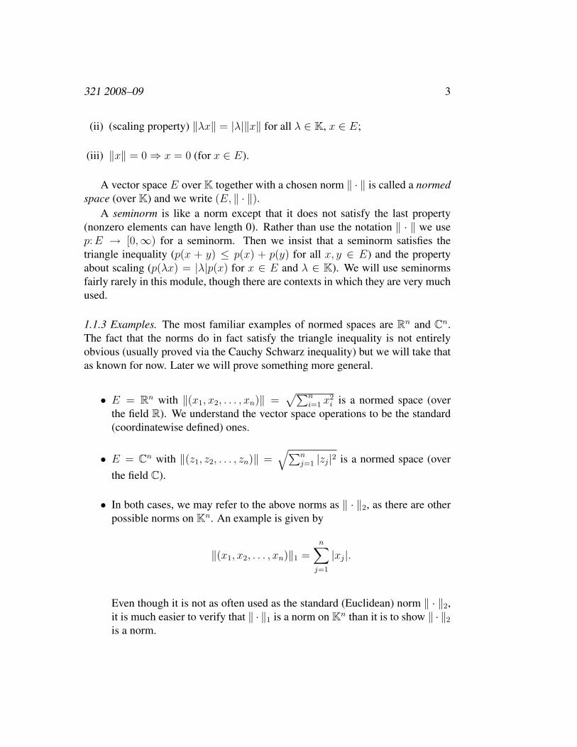
(ii) (scaling property) ‖λx‖ = |λ|‖x‖ for all λ ∈ K, x ∈ E;

(iii) ‖x‖ = 0 ⇒ x = 0 (for x ∈ E).

A vector space E over K together with a chosen norm ‖ · ‖ is called a normedspace (over K) and we write (E, ‖ · ‖).

A seminorm is like a norm except that it does not satisfy the last property(nonzero elements can have length 0). Rather than use the notation ‖ · ‖ we usep: E → [0,∞) for a seminorm. Then we insist that a seminorm satisfies thetriangle inequality (p(x + y) ≤ p(x) + p(y) for all x, y ∈ E) and the propertyabout scaling (p(λx) = |λ|p(x) for x ∈ E and λ ∈ K). We will use seminormsfairly rarely in this module, though there are contexts in which they are very muchused.

1.1.3 Examples. The most familiar examples of normed spaces are Rn and Cn.The fact that the norms do in fact satisfy the triangle inequality is not entirelyobvious (usually proved via the Cauchy Schwarz inequality) but we will take thatas known for now. Later we will prove something more general.

• E = Rn with ‖(x1, x2, . . . , xn)‖ =√∑n

i=1 x2i is a normed space (over

the field R). We understand the vector space operations to be the standard(coordinatewise defined) ones.

• E = Cn with ‖(z1, z2, . . . , zn)‖ =√∑n

j=1 |zj|2 is a normed space (overthe field C).

• In both cases, we may refer to the above norms as ‖ · ‖2, as there are otherpossible norms on Kn. An example is given by

‖(x1, x2, . . . , xn)‖1 =n∑

j=1

|xj|.

Even though it is not as often used as the standard (Euclidean) norm ‖ · ‖2,it is much easier to verify that ‖ · ‖1 is a norm on Kn than it is to show ‖ · ‖2

is a norm.


1.2 Metric spacesThis subsection may be largely review of material from module 221 apart fromLemma 1.2.7 below.

1.2.1 Definition. If X is a set and d: X ×X → [0,∞) ⊂ R is a function with theproperties:

(i) d(x, y) ≥ 0 (for x, y ∈ X);

(ii) d(x, y) = d(y, x) (for x, y ∈ X);

(iii) d(x, z) ≤ d(x, y) + d(y, z) (triangle inequality) for x, yz, zinX;

(iv) x, y ∈ X and d(x, y) = 0 → x = y,

we say d is a metric, and the combination (X, d) is called a metric space.If we omit the last condition that d(x, y) = 0 implies x = y, we call d a

pseudometric or semimetric.

1.2.2 Notation. In any metric space (X, d) we define open balls as follows. Fixany point x0 ∈ X (which we think of as the centre) and any r > 0. Then the openball of radius r centre x0 is

B(x0, r) = {x ∈ X : d(x, x0) < r}.

The closed ball with the same centre and radius is

B(x0, r) = {x ∈ X : d(x, x0) ≤ r}.

1.2.3 Open and closed subsets. A set G ⊆ X (where we now understand that(X, d) is a particular metric space) is open if each x ∈ G is an interior point of G.

A point x ∈ G is called an interior point of G if there is a ball B(x, r) ⊂ Gwith r > 0.

Picture for an open set: G contains none of its ‘boundary’ points.Any union G =

⋃i∈I Gi of open sets Gi ⊆ X is open (I any index set,

arbitrarily large).F ⊆ X is closed if its complement X \ F is open.Picture for a closed set: F contains all of its ‘boundary’ points.Note that open and closed are opposite extremes. There are plenty of sets

which are neither open nor closed. For example {z = x + iy ∈ C : 1 ≤ x, y < 2}is a square in the plane C = R2 with some of the ‘boundary’ included and somenot. It is neither open nor closed.

321 2008–09 5

Any intersection F =⋃

i∈I Fi of closed sets Fi ⊂ X is closed.Finite intersection G1 ∩G2 ∩ · · · ∩Gn of open sets are open.Finite unions of closed sets are closed.

1.2.4 Exercise. Show that an open ball B(x0, r) in a metric space (X, d) is anopen set.

1.2.5 Interiors and closures. Fix a metric space (X, d).For any set E ⊆ X , the interior E◦ is the set of all its interior points.

E◦ = {x ∈ E : ∃r > 0 with B(z, r) ⊆ E}

is the largest open subset of X contained in E. Also

E◦ =⋃{G : G ⊆ E, G open in C}

Picture: E◦ is E minus all its ‘boundary’ points.The closure of E is

E =⋂{F : F ⊂ X, E ⊂ F and F closed}

and it is the smallest closed subset of X containing E.Picture: E is E with all its ‘boundary’ points added.Properties: E = X \ (X \ E)◦ and E◦ = X \ (X \ E).

1.2.6 Boundary. Again we assume we have a fixed metric space (X, d) in whichwe work.

The boundary ∂E of a set E ⊆ X is defined as ∂E = E \ E◦.This formal definition makes the previous informal pictures into facts.

1.2.7 Lemma. On any normed space (E, ‖·‖) we can define a metric via d(x, y) =‖x− y‖.


From the metric we also get a topology (notion of open set).In a similar way a seminorm p on E gives rise to a pseudo metric ρ(x, y) =

p(x − y) (like a metric but ρ(x, y) = 0 is allowed for x 6= y). From a pseudometric, we get a (non Hausdorff) topology by saying that a set is open if it containsa ball Bρ(x0, r) = {x ∈ E : ρ(x, x0) < r} of some positive radius r > 0 abouteach of its points.

Proof. It is easy to check that d as defined satisfies the properties for a metric.

• d(x, y) = ‖x− y‖ ∈ [0,∞)

• d(x, y) = ‖x− y‖ = ‖(−1)(y − x)‖ = | − 1|‖y − x‖ = d(y, x)

• d(x, z) = ‖x − z‖ = ‖(x − y) + (y − z)‖ ≤ ‖x − y‖ + ‖y − z‖ =d(x, y) + d(y, z)

• d(x, y) = 0 ⇒ ‖x− y‖ = 0 ⇒ x− y = 0 ⇒ x = y.

The fact that pseudo metrics give rise to a topology is quite easy to verify.

1.2.8 Continuity. Let (X, dX) and (Y, dY ) be two metric spaces.If f : X → Y is a function, then f is called continuous at a point x0 ∈ X if for

each ε > 0 it is possible to find δ > 0 so that

x ∈ X, dX(x, x0) < δ ⇒ dY (f(x), f(x0)) < ε

f : X → Y is called continuous if it is continuous at each point x0 ∈ X .

1.2.9 Example. If (X, d) is a metric space and f : X → R is a function, then whenwe say f is continuous we mean that it is continuous from the metric space X tothe metric space R = R with the normal absolute value metric.

Similarly for complex valued functions f : X → C, we normally think of con-tinuity to mean the situation where C has the usual metric.

1.2.10 Proposition. If f : X → Y is a function between two metric spaces X andY , then f is continuous if and only if it satisfies the following condition: for eachopen set U ⊂ Y , its inverse image f−1(U) = {x ∈ X : f(x) ∈ U} is open in X .

Proof. Exercise.

321 2008–09 7

1.2.11 Limits. We now define limits of sequences in a metric space (X, d). Asequence (xn)∞n=1 in X is actually a function x: N → X from the natural numbersN = {1, 2, . . .} to X where, by convention, we use the notation xn instead of theusual function notation x(n).

To say limn→∞ xn = ` (with ` ∈ X also) means:

for each ε > 0 it is possible to find N ∈ N so that

n ∈ N, n > N ⇒ d(xn, `) < ε.

An important property of limits of sequences in metric spaces is that a se-quence can have at most one limit. In a way we have almost implicitly assumedthat by writing limn→∞ xn as though it is one thing. Notice however that there aresequences with no limit.

1.2.12 Proposition. Let X be a metric space, S ⊂ X and x ∈ X . Then x ∈S ⇐⇒ there exists a sequence (sn)∞n=1 with sn ∈ S for all n and limn→∞ sn = x(in X).

Proof. Not given here. (Exercise.)

1.2.13 Proposition. Let X and Y be two metric spaces. If f : X → Y is a functionand x0 ∈ X is a point, then f is continuous at x0 if and only if limn→∞ f(xn) =f(z0) holds for all sequences (xn)∞n=1 in X with limn→∞ xn = x0.

Proof. Not given here. (Exercise.)

1.2.14 Remark. Consider the case where we have sequences in R, which is notonly a metric space but where we can add and multiply.

One can show that the limit of a sum is the sum of the limits (provided theindividual limits make sense). More symbolically,

limn→∞

xn + yn = limn→∞

xn + limn→∞

yn.

Similarlylim

n→∞xnyn =

(lim

n→∞xn

)(lim

n→∞yn

).

if both individual limits exist.We also have the result on limits of quotients,

limn→∞

xn

yn

=limn→∞ xn

limn→∞ yn


provided limn→∞ yn 6= 0. In short the limit of a quotient is the quotient of thelimits provided the limit in the denominator is not zero.

One can use these facts to show that sums and products of continuous R-valued functions on metric spaces are continuous. Quotients also if no division by0 occurs.

1.2.15 Definition. If X is a set then a topology T on X is a collection of subsetsof X with the following properties

(i) φ ∈ T and X ∈ T ;

(ii) if Ui ∈ T for all i ∈ I = some index set, then⋃

i∈I Ui ∈ T ;

(iii) if U1, U2 ∈ T , then U1 ∩ U2 ∈ T .

A set X together with a topology T on X is called a topological space (X, T ).

1.2.16 Remark. Normally, when we consider a topological space (X, T ), we referto the subsets of X that are in T as open subsets of X .

We should perhaps explain immediately that if we start with a metric space(X, d) and if we take T to be the open subsets of (X, d) (according to the defini-tion we gave earlier), then we get a topology T on X .

Notice that at least some of the concepts we had for metric spaces can beexpressed using only open sets without the necessity to refer to distances.

• F ⊂ X is closed ⇐⇒ X \ F is open

• f : X → Y is continuous ⇐⇒ f−1(U) is open in X whenever U is openin Y .

1.2.17 Example. (i) One example of a topology on any set X is the topologyT = P(X) = the power set of X (all subsets of X are in T , all subsetsdeclared to be open).

We can also get to this topology from a metric, where we define

d(x1, x2) =

{0 if x1 = x2

1 if x1 6= x2

In this metric the open ball of radius 1/2 about any point x0 ∈ X is

B(x0, 1/2) = {x0}

321 2008–09 9

and all one points sets are then open. As unions of open sets are open, itfollows that all subsets are open.

The metric is called the discrete metric and the topology is called the discretetopology.

All functions f : X → Y will be continuous if X has the discrete topology(and Y can have any valid topology).

(ii) The other extreme is to take (say when X has at least 2 elements) T ={∅, X}. This is a valid topology, called the indiscrete topology.

If X has at least two points x1 6= x2, there can be no metric on X that givesrise to this topology. If we thought for a moment we had such a metric d, wecan take r = d(x1, x2)/2 and get an open ball B(x1, r) in X that contains x1

but not x2. As open balls in metric spaces are in fact open subsets, we musthave B(x1, r) different from the empty set and different from X .

The only functions f : X → R that are continuous are the constant functionsin this example. On the other hand every function g: Y → X is continuous(no matter what Y is, as long as it is a topological space so that we can saywhat continuity means).

This example shows that there are topologies that do not come from metrics,or topological spaces where there is no metric around that would give thesame idea of open set. Or, in other language, topological spaces that do notarise from metric spaces (are not metric spaces). Our example is not veryconvincing, however. It seems very silly, perhaps. If we studied topologicalspaces in a bit more detail we would come across more significant examplesof topological spaces that are not metric spaces (and where the topologydoes not arise from any metric).

1.2.18 Compactness. Let (X, d) be a metric space.Let T ⊆ X . An open cover of T is a family U of open subsets of X such that

T ⊆⋃{U : U ∈ U}

A subfamily V ⊆ U is called a subcover of U if V is also a cover of T .T is called compact if each open cover of T has a finite subcover.T is called bounded if there exists R ≥ 0 and x0 ∈ X with T ⊆ B(x0, R).One way to state the Heine-Borel theorem is that a subset T ⊆ Rn is compact

if and only if it is both (1) closed and (2) bounded.


Continuous images of compact sets are compact: T ⊆ X compact, f : T → Ycontinuous implies f(T ) compact.

1.2.19 Definition. If (X, d) is a metric space, then a subset T ⊂ X is calledsequentially compact if it has the following property:

Each sequence (tn)∞n=1 has a subsequence (tnj)∞j=1 with limj→∞ tnj

=` ∈ T for some ` ∈ T .

In words, every sequence in T has a subsequence with a limit in T .

1.2.20 Theorem. In a metric space (X, d) a subset T ⊂ X is compact if and onlyif it is sequentially compact.

Proof. Omitted here.

1.2.21 Remark. We can abstract almost all of the above statements about compact-ness to general topological spaces rather than a metric space. Metric spaces arecloser to what we are familiar with, points in space or the plane or the line, wherewe think we can see geometrically what distance means (straight line distancebetween points).

At least in normed spaces, many familiar ideas still work in some form.One thing to be aware of is that sequences are not as useful in topologi-

cal spaces as they are in metric spaces. Sequences in a topological space mayconverge to more than one limit. Compactness (defined via open covers) is notthe same as sequential compactness in every topological space. Sequences donot always describe closures or continuity as they do in metric spaces (Proposi-tions 1.2.12 and 1.2.13).

1.3 Examples of normed spaces1.3.1 Examples. (i) Kn with the standard Euclidean norm is complete.

(ii) If X is a metric space (or a topological space) we can define a norm onE = BC(X) = {f : X → K : f bounded and continuous} by

‖f‖ = supx∈X

|f(x)|.

To be more precise, we have to have a vector space before we can have anorm. We define the vector space operations on BC(X) in the ‘obvious’(pointwise) way. Here are the definition of f + g and λf for f, g ∈ BC(X),λ ∈ K:

321 2008–09 11

• (f + g)(x) = f(x) + g(x) (for x ∈ X)

• (λf)(x) = λ(f(x)) = λf(x) (for x ∈ X)

We should check that f + g, λf ∈ BC(X) always and that the vector spacerules are satisfied, but we leave this as an exercise if you have not seen itbefore.

It is not difficult to check that we have defined a norm on BC(X). It isknown often as the ‘uniform norm’ or the ‘sup norm’ (on X).

(iii) If we replace X by a compact Hausdorff space K in the previous example,we know that every continuous f : K → K is automatically bounded. Theusual notation then is to use C(K) rather than BC(K).

Otherwise everything is the same (vector space operations, supremum norm).

(iv) If we take for X the discrete space X = N, we can consider the exampleBC(N) as a space of functions on N (with values in K). However, it is moreusual to think in terms of this example as a space of sequences. The usualnotation for it is

`∞ = {(xn)∞n=1 : xn ∈ K∀n and supn|xn| < ∞}.

So `∞ is the space of all bounded (infinite) sequences of scalars. The vectorspace operations on sequences are defined as for functions (pointwise orterm-by-term)

(xn)∞n=1 + (yn)∞n=1 = (xn + yn)∞n=1

λ(xn)∞n=1 = (λxn)∞n=1

and the uniform or supremum norm on `∞ is typically denoted by a subscript∞ (to distinguish it from other norms on other sequence spaces that we willcome to soon).

‖(xn)∞n=1‖∞ = supn|xn|.

It will be important for us to deal with complete normed spaces (which arecalled Banach spaces). First we will review some facts about complete metricspaces and completions. A deeper consequence of completeness is the Baire cat-egory theorem.

Completeness is important if one wants to prove that equations have a solution,one technique is to produce a sequence of approximate solutions. If the space is


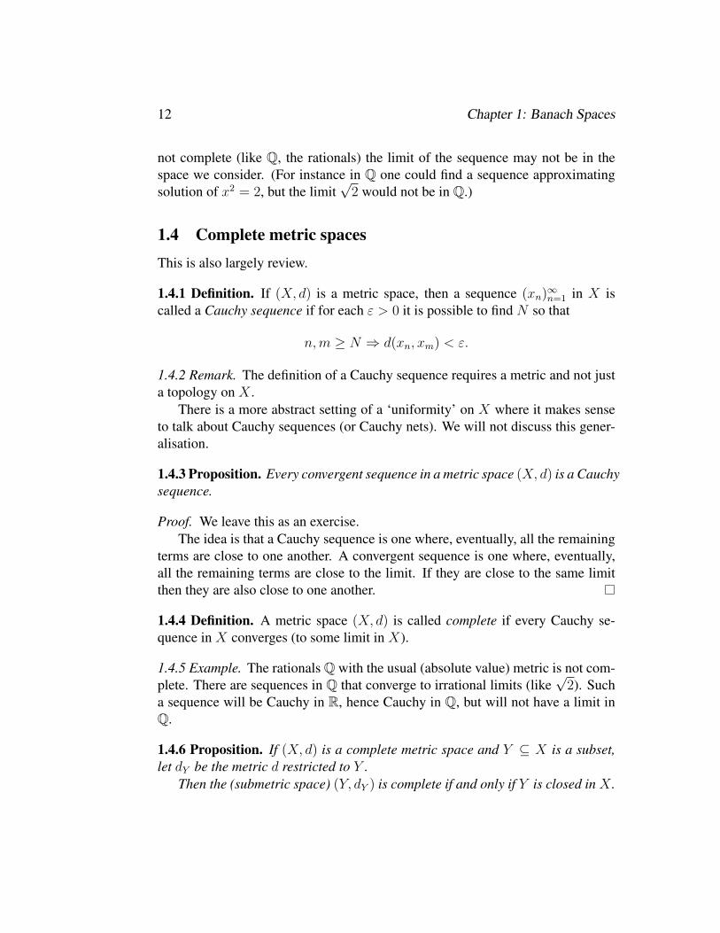
not complete (like Q, the rationals) the limit of the sequence may not be in thespace we consider. (For instance in Q one could find a sequence approximatingsolution of x2 = 2, but the limit

√2 would not be in Q.)

1.4 Complete metric spacesThis is also largely review.

1.4.1 Definition. If (X, d) is a metric space, then a sequence (xn)∞n=1 in X iscalled a Cauchy sequence if for each ε > 0 it is possible to find N so that

n, m ≥ N ⇒ d(xn, xm) < ε.

1.4.2 Remark. The definition of a Cauchy sequence requires a metric and not justa topology on X .

There is a more abstract setting of a ‘uniformity’ on X where it makes senseto talk about Cauchy sequences (or Cauchy nets). We will not discuss this gener-alisation.

1.4.3 Proposition. Every convergent sequence in a metric space (X, d) is a Cauchysequence.

Proof. We leave this as an exercise.The idea is that a Cauchy sequence is one where, eventually, all the remaining

terms are close to one another. A convergent sequence is one where, eventually,all the remaining terms are close to the limit. If they are close to the same limitthen they are also close to one another.

1.4.4 Definition. A metric space (X, d) is called complete if every Cauchy se-quence in X converges (to some limit in X).

1.4.5 Example. The rationals Q with the usual (absolute value) metric is not com-plete. There are sequences in Q that converge to irrational limits (like

√2). Such

a sequence will be Cauchy in R, hence Cauchy in Q, but will not have a limit inQ.

1.4.6 Proposition. If (X, d) is a complete metric space and Y ⊆ X is a subset,let dY be the metric d restricted to Y .

Then the (submetric space) (Y, dY ) is complete if and only if Y is closed in X .

321 2008–09 13

Proof. Suppose first (Y, dY ) is complete. If x0 is a point of the closure of Y inX , then there is a sequence (yn)∞n=1 of points yn ∈ Y that converges (in X) tox0. The sequence (yn)∞n=1 is then Cauchy in (X, d). But the Cauchy conditioninvolves only distances d(yn, ym) = dY (yn, ym) between the terms and so (yn)∞n=1

is Cauchy in Y . By completeness there is y0 ∈ Y so that yn → y0 as n →∞. Thatmeans limn→∞ dY (yn, y0) = 0 and that is the same as limn→∞ d(yn, y0) = 0 oryn → yo when we consider the sequence and the limit in X . Since also yn → x0

as n → ∞, and limits in X are unique, we conclude x0 = y0 ∈ Y . Thus Y isclosed in X .

Conversely, suppose Y is closed in X . To show Y is complete, consider aCauchy sequence (yn)∞n=1 in Y . It is also Cauchy in X . As X is complete thesequence has a limit x0 ∈ X . But we must have x0 ∈ Y because Y is closed inX . So the sequence (yn)∞n=1 converges in (Y, dY ).

1.4.7 Remark. The following lemma is useful in showing that metric spaces arecomplete.

1.4.8 Lemma. Let (X, d) be a metric space in which each Cauchy sequence hasa convergent subsequence. Then (X, d) is complete.

Proof. We leave this as an exercise.The idea is that as the terms of the whole sequence are eventually all close to

one another, and the terms of the convergent subsequence are eventually close tothe limit ` of the subsequence, the terms of the whole sequence must be eventuallyclose to `.

1.4.9 Corollary. Compact metric spaces are complete.

1.4.10 Definition. If (X, dX) and (Y, dY ) are metric spaces, then a function f : X →Y is called uniformly continuous if for each ε > 0 it is possible to find δ > 0 sothat

x1, x2 ∈ X, dX(x1, x2) < δ ⇒ dY (f(x1), f(x2)) < ε.

1.4.11 Proposition. Uniformly continuous functions are continuous.

Proof. We leave this as an exercise.The idea is that in the ε-δ criterion for continuity, we fix one point (say x1) as

well as ε > 0 and then look for δ > 0. In uniform continuity, the same δ > 0 mustwork for all x1 ∈ X .


1.4.12 Definition. If (X, dX) and (Y, dY ) are metric spaces, then a function f : X →Y is called an isometry if dY (f(x1), f(x2)) = dX(x1, x2) for all x1, x2 ∈ X .

We could call f distance preserving instead of isometric, but the word isomet-ric is more commonly used. Sometimes we consider isometric bijections (whichthen clearly have isometric inverse maps). If there exists an isometric bijectionbetween two metric spaces X and Y , we can consider them as equivalent metricspaces (because every property defined only in terms of the metric must be sharedby Y is X has the property).

1.4.13 Example. Isometric maps are injective and uniformly continuous.

Proof. Let f : X → Y be the map. To show injective, let x1, x2 ∈ X with x1 6= x2.Then dX(x1, x2) > 0 ⇒ dY (f(x1), f(x2)) > 0 ⇒ f(x1) 6= f(x2).

To show uniform continuity, take δ = ε.

1.4.14 Definition. If (X, TX) and (Y, TY ) are topological spaces (or (X, dX) and(Y, dY ) are metric spaces) then a homeomorphism from X onto Y is a bijectionf : X → Y with f continuous and f−1 continuous.

1.4.15 Remark. If f : X → Y is a homeomorphism of topological spaces, thenV ⊂ Y open implies U = f−1(V ) ⊂ X open (by continuity of f ). On the otherhand U ⊂ X open implies (f−1)−1(U) = f(U) open by continuity of f−1 (sincethe inverse image of U under the inverse map f−1 is the same as the forward imagef(U)). In this way we can say that

U ⊂ X is open ⇐⇒ f(U) ⊂ Y is open

and homeomorphic spaces are identical from the point of view of topologicalproperties.

Note that isometric metric spaces are identical from the point of view of metricproperties. The next next result says that completeness transfers between metricspaces that are homeomorphic via a homeomorphism that is uniformly continuousin one direction.

1.4.16 Proposition. If (X, dX) and (Y, dY ) are metric spaces with (X, dX) com-plete, and f : X → Y is a homeomorphism with f−1 uniformly continuous, then(Y, dY ) is also complete.

Proof. Let (yn)∞n=1 be a Cauchy sequence in Y . Let xn = f−1(yn). We claim(xn)∞n=1 is Cauchy in X . Given ε > 0 find δ > 0 by uniform continuity of f−1 sothat

y, y′ ∈ Y, dY (y, y′) < δ ⇒ dX(f−1(y), f−1(y′)) < ε.

321 2008–09 15

As (yn)∞n=1 is Cauchy in Y , there is N > 0 so that

n, m ≥ N ⇒ dY (yn, ym) < δ.

Combining these, we see

n, m ≥ N ⇒ dX(f−1(yn), f−1(ym)) < ε.

So (xn)∞n=1 is Cauchy in X , and so has a limit x0 ∈ X . By continuity of f atx0, we get f(xn) = yn → f(x0) as n → ∞. So (yn)∞n=1 converges in Y . Thisshows that Y is complete.

1.4.17 Example. There are homeomorphic metric spaces where one is completeand the other is not. For example, R is homeomorphic to the open unit interval(0, 1).

One way to see this is to take g: R → (0, 1) as g(x) = (1/2) + (1/π) tan−1 x.Another is g(x) = (1/2) + x/(2(1 + |x|)).

In the standard absolute value distance R is complete but (0, 1) is not.One can use a specific homeomorphism g: R → (0, 1) to transfer the distance

from R to (0, 1). Define a new distance on (0, 1) by ρ(x1, x2) = |g−1(x1) −g−1(x2)|. With this distance ρ on (0, 1), the map g becomes an isometry and so(0, 1) is complete in the ρ distance.

The two topologies we get on (0, 1), from the standard metric and from themetric ρ, will be the same. We can see from this example that completeness is nota topological property.

1.4.18 Theorem ((Banach) contraction mapping theorem). Let (x, d) be a (nonempty)complete metric space and let f : X → X be a strictly contractive mapping (whichmeans there exists 0 ≤ r < 1 so that d(f(x1), f(x2)) ≤ rd(x1, x2) holds for allx1, x2 ∈ X).

Then f has a unique fixed point in X (that is there is a unique x ∈ X withf(x) = x.

Proof. We omit this proof as we will not use this result. It can be used to showthat certain ordinary differential equations have (local) solutions.

The idea of the proof is to start with x0 ∈ X arbitrary and to define x1 =f(x0), x2 = f(x1) etc., that is xn+1 = f(xn) for each n. The contractive propertyimplies that (xn)∞n=1 is a Cauchy sequence. The limit limn→∞ xn is the fixed pointx. Uniqueness of the fixed point follows from the contractive property.


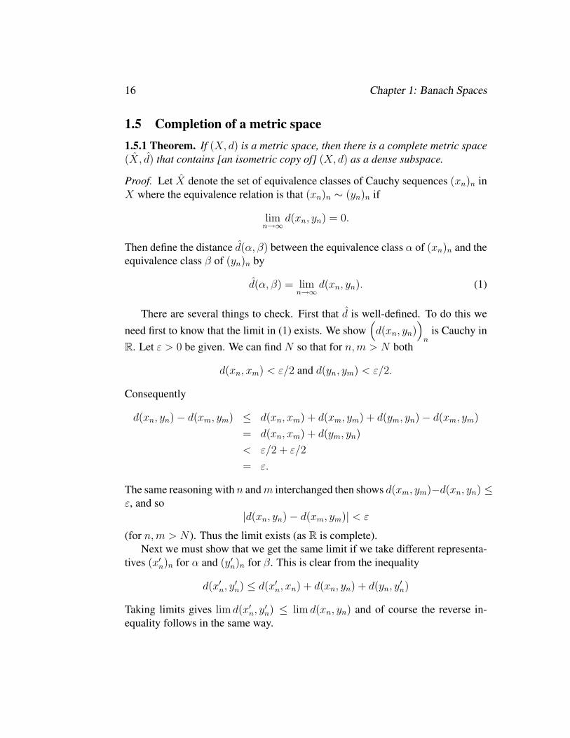
1.5 Completion of a metric space1.5.1 Theorem. If (X, d) is a metric space, then there is a complete metric space(X, d) that contains [an isometric copy of] (X, d) as a dense subspace.

Proof. Let X denote the set of equivalence classes of Cauchy sequences (xn)n inX where the equivalence relation is that (xn)n ∼ (yn)n if

limn→∞

d(xn, yn) = 0.

Then define the distance d(α, β) between the equivalence class α of (xn)n and theequivalence class β of (yn)n by

d(α, β) = limn→∞

d(xn, yn). (1)

There are several things to check. First that d is well-defined. To do this we

need first to know that the limit in (1) exists. We show(d(xn, yn)

)n

is Cauchy inR. Let ε > 0 be given. We can find N so that for n, m > N both

d(xn, xm) < ε/2 and d(yn, ym) < ε/2.

Consequently

d(xn, yn)− d(xm, ym) ≤ d(xn, xm) + d(xm, ym) + d(ym, yn)− d(xm, ym)

= d(xn, xm) + d(ym, yn)

< ε/2 + ε/2

= ε.

The same reasoning with n and m interchanged then shows d(xm, ym)−d(xn, yn) ≤ε, and so

|d(xn, yn)− d(xm, ym)| < ε

(for n, m > N ). Thus the limit exists (as R is complete).Next we must show that we get the same limit if we take different representa-

tives (x′n)n for α and (y′n)n for β. This is clear from the inequality

d(x′n, y′n) ≤ d(x′n, xn) + d(xn, yn) + d(yn, y

′n)

Taking limits gives lim d(x′n, y′n) ≤ lim d(xn, yn) and of course the reverse in-

equality follows in the same way.

321 2008–09 17

Next we must check that d is a metric on X . This is quite straightforward.To show that there is a copy of (X, d) in X is also easy — the (equivalence

classes of the) constant sequences

x, x, x, . . . (x ∈ X)

give the required copy.To show that this copy is dense in X , take an arbitrary α ∈ X and let the

Cauchy sequence (xn)n be a representative for α. Let αj denote the equivalenceclass of the constant sequence xj, xj, xj, . . .. From the Cauchy condition it is easyto see that d(αj, α) → 0 as j →∞.

The final step is to show that (X, d) is complete. Take a Cauchy sequence(αj)j in X . Passing to a subsequence (by observation 1.4.8 it is enough to find aconvergent subsequence), we can suppose that

d(αj, αj+1) ≤1

2jfor j = 1, 2, 3, . . .

Let (xjn)n = (xj1, xj2, . . .) represent αj . Choose first Nj so that

n, m ≥ Nj ⇒ d(xjn, xjm) <1

j

and also choose N ′j so that

n ≥ N ′j ⇒ d(xjn, xj+1 n) <

1

2j

Then put nj = max(Nj, N′j). By making the nj larger, if necessary, we can

assume that n1 < n2 < n3 < · · ·.Define yk = xknk

and let α denote the equivalence class of (yn)n. We claimthat αj → α as j →∞, but first we must verify that (yk)k is a Cauchy sequence,so that we can be sure it made sense to refer to its equivalence class.

For k, ` > 0,

d(yk, yk+`) = d(xknk, xk+` nk+`

)

≤ d(xknk, xknk+`

) + d(xknk+`, xk+` nk+`

)

≤ 1

k+

k+`−1∑p=k

1

2p

<1

k+

1

2k−1

→ 0 as k →∞.


This verifies that (yk)k is Cauchy.Finally, to verify that αj → α, note that for k ≥ nj ,

d(xjk, yk) = d(xjk, xknk)

≤ d(xjk, xjnk) + d(xjnk

, xknk)

≤ 1

j+

k−1∑`=j

1

2`

≤ 1

j+

1

2j−1

Therefore d(αj, α) ≤ 1

j+

1

2j−1

→ 0 as j →∞.

This finishes the proof that every metric space (X, d) has a completion.

1.5.2 Remark. To prove that the completion is unique (up to a distance preservingbijection that keeps the copy of X ‘fixed’) requires just a little more work.

It relies on the fact that a uniformly continuous function on a dense subset X0

of one metric space X , with values in a complete metric space Y , has a uniquecontinuous extension to a function : X → Y .1.5.3 Remark. One can also show that the completion of a normed space can beturned into a normed space. This requires defining vector space operations on(equivalence classes) of Cauchy sequences from the normed space. We do thisby adding the sequences term by term, and multiplying each term by the scalar.There is checking required — to show that the operations are well defined forequivalence classes. Then we have to define a norm on the completion (whichis the distance to the origin in the completion — need to check it satisfies theconditions for a norm and that the norm and distance are related by d(α, β) =‖α− β‖. None of the steps are difficult to carry out in detail.

1.6 Baire Category Theorem1.6.1 Definition. A subset S ⊂ X of a metric space (X, d) is called nowheredense if the interior of its closure is empty, (S)◦ = ∅.

A subset E ⊂ X is called of first category if it is a countable union of nowheredense subsets, that is, the union E =

⋃∞n=1 Sn of a sequence of nowhere dense

sets Sn) ((Sn)◦ = ∅∀n).A subset Y ⊂ X is called of second category if it fails to be of first category.

321 2008–09 19

1.6.2 Example. (a) If a singleton subset S = {s} ⊂ X (X metric) fails to benowhere dense, then the interior of its closure is not empty. The closure S =S = {s} and if that has any interior it means it contains a ball of some positiveradius r > 0. So

Bd(s, r) = {x ∈ X : d(x, s) < r} = {s}

and this means that s is an isolated point of X (no points closer to it than r).

An example where this is possible would be X = Z with the usual distance(so B(n, 1) = {n}) and S any singleton subset. Another example is X =B((2, 0), 1) ∪ {0} ⊂ R2 (with the distance on X being the same as the usualdistance between points in R2) and S = {0}.

(b) In many cases, there are no isolated points in X , and then a one point set isnowhere dense. So a countable subset is then of first category (S = {s1, s2, . . .}where the elements can be listed as a finite or infinite sequence).

For example S = Z is of first category as a subset of R, though it of secondcategory as a subset of itself. S = Q is of first category both in R and in itself(because it is countable and points are not isolated).

The idea is that first countable means ‘small’ in some sense, while secondcategory is ‘not small’ in the same sense. While it is often not hard to see that aset is of first category, it is harder to see that it fails to be of first category. Onehas to consider all possible ways of writing the set as a union of a sequenceof subsets.

1.6.3 Theorem (Baire Category). Let (X, d) be a complete metric space which isnot empty. Then the whole space S = X is of second category in itself.

Proof. If not, then X is of first category and that means X =⋃∞

n=1 Sn where eachSn is a nowhere dense subset Sn ⊂ X (with (Sn)◦ = ∅).

Since Sn has empty interior, its complement is a dense open set. That is

X \ Sn = X \ (Sn)◦ = X

Thus if we take any ball Bd(x, r) in X , there is a point y ∈ (X \ Sn) ∩ Bd(x, r)and then because X \ Sn is open there is a (smaller) δ > 0 with Bd(y, δ) ⊂(X \ Sn) ∩ Bd(x, r). In fact, making δ > 0 smaller again, there is δ > 0 withB(y, δ) ⊂ (X \ Sn) ∩Bd(x, r).


Start with x0 ∈ X any point and r0 = 1. Then, by the above reasoning thereis a ball

Bd(x1, r1) = {x ∈ X : d(x, x1) ≤ r1} ⊂ (X \ S1) ∩Bd(x0, r0)

and r1 < r0/2 ≤ 1/2. We can then find x2 and r2 ≤ r1/2 < 1/22 so that

Bd(x2, r2) ⊂ (X \ S2) ∩Bd(x1, r1)

and we can continue this process to select x1, x2, . . . and r1, r2, . . . with

0 < rn ≤ rn−1/2 <1

2n, Bd(xn, rn) ⊂ (X\Sn)∩Bd(xn−1, rn−1) (n = 1, 2, . . .)

We claim the sequence (xn)∞n=1 is a Cauchy sequence in X . This is becausem ≥ n ⇒ xm ∈ Bd(xn, rn) ⇒ d(xm, xn) < rn < 1/2n. So, if n, m are bothlarge

d(xm, xn) < min

(1

2n,

1

2m

)is small.

By completeness, x∞ = limn→∞ xn exists in X . Since the closed ball Bd(xn, rn)is a closed set in X and contains all xm for m ≥ n, it follows that x ∈ Bd(xn, rn)for each n. But Bd(xn, rn) ⊂ X \ Sn and so x /∈ Sn. This is true for all n and sowe have the contradiction

x /∈∞⋃

n=1

Sn = X

Thus X cannot be a union of a sequence of nowhere dense subsets.

1.6.4 Corollary. Let (X, d) be a compact metric space. Then the whole spaceS = X is of second category in itself.

Proof. Compact metric spaces are complete. So this follows from the theorem.

1.7 Banach spaces1.7.1 Definition. A normed space (E, ‖ · ‖) (over K) is called a Banach space(over K) if E is complete in the metric arising from the norm.

321 2008–09 21

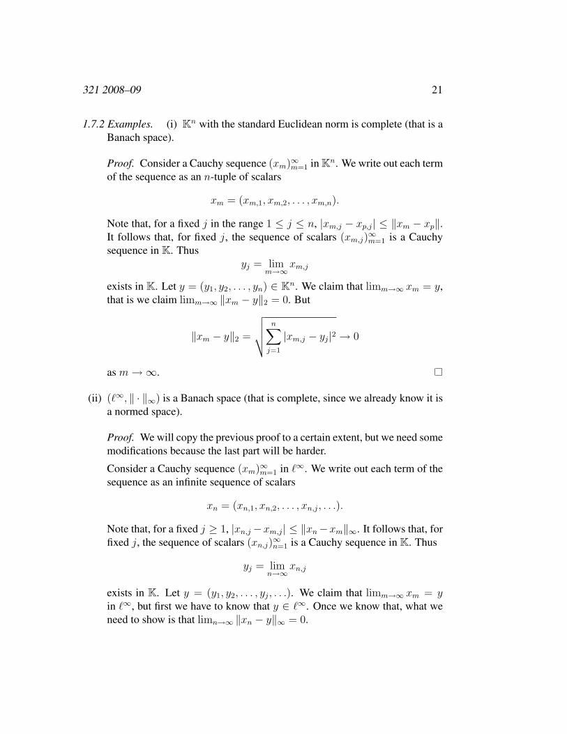
1.7.2 Examples. (i) Kn with the standard Euclidean norm is complete (that is aBanach space).

Proof. Consider a Cauchy sequence (xm)∞m=1 in Kn. We write out each termof the sequence as an n-tuple of scalars

xm = (xm,1, xm,2, . . . , xm,n).

Note that, for a fixed j in the range 1 ≤ j ≤ n, |xm,j − xp,j| ≤ ‖xm − xp‖.It follows that, for fixed j, the sequence of scalars (xm,j)

∞m=1 is a Cauchy

sequence in K. Thusyj = lim

m→∞xm,j

exists in K. Let y = (y1, y2, . . . , yn) ∈ Kn. We claim that limm→∞ xm = y,that is we claim limm→∞ ‖xm − y‖2 = 0. But

‖xm − y‖2 =

√√√√ n∑j=1

|xm,j − yj|2 → 0

as m →∞.

(ii) (`∞, ‖ · ‖∞) is a Banach space (that is complete, since we already know it isa normed space).

Proof. We will copy the previous proof to a certain extent, but we need somemodifications because the last part will be harder.

Consider a Cauchy sequence (xm)∞m=1 in `∞. We write out each term of thesequence as an infinite sequence of scalars

xn = (xn,1, xn,2, . . . , xn,j, . . .).

Note that, for a fixed j ≥ 1, |xn,j −xm,j| ≤ ‖xn−xm‖∞. It follows that, forfixed j, the sequence of scalars (xn,j)

∞n=1 is a Cauchy sequence in K. Thus

yj = limn→∞

xn,j

exists in K. Let y = (y1, y2, . . . , yj, . . .). We claim that limm→∞ xm = yin `∞, but first we have to know that y ∈ `∞. Once we know that, what weneed to show is that limn→∞ ‖xn − y‖∞ = 0.


To show y ∈ `∞, we start with the Cauchy condition for ε = 1. It says thatthere exists N ≥ 1 so that

n, m ≥ N ⇒ ‖xn − xm‖∞ < 1

Taking n = N we get

m ≥ N ⇒ ‖xN − xm‖∞ < 1

Since |xN,j − xm,j| ≤ ‖xN − xm‖∞ it follows that for each j ≥ 1 we have

m ≥ N ⇒ |xN,j − xm,j| < 1

Letting m →∞, we find that |xN,j − yj| ≤ 1. Thus

|yj| ≤ |xN,j − yj|+ |xN,j| ≤ 1 + ‖xN‖∞

holds for j ≥ 1 and so supj |yj| < ∞. We have verified that y ∈ `∞.

To show that limn→∞ ‖xn − y‖∞ = 0, we start with ε > 0 and apply theCauchy criterion to find N = Nε ≥ 1 (not the same N as before) so that

n, m ≥ N ⇒ ‖xn − xm‖∞ <ε

2

Hence, for any j ≥ 1 we have

n, m ≥ N ⇒ |xn,j − xm,j| ≤ ‖xn − xm‖∞ <ε

2

Fix any n ≥ N and let m →∞ to get

|xn,j − yj| = limm→∞

|xn,j − xm,j| ≤ε

2

So we have

n ≥ N ⇒ ‖xn − y‖∞ = supj≥1

|xn,j − yj| ≤ε

2< ε

This shows limn→∞ ‖xn − y‖∞ = 0, as required.

(iii) If X is a topological space then (BC(X), ‖ · ‖∞) is a Banach space.

(Note that this includes `∞ = BC(N) as a special case. The main differenceis that we need to worry about continuity here.)

321 2008–09 23

Convergence of sequences in the supremum norm corresponds touniform convergence on X . (See §A.1 for the definition and afew useful facts about uniform convergence.)

Proof. (of the assertion about uniform convergence).

Suppose (fn)∞n=1 is a sequence of functions in BC(X) and g ∈ BC(X).

First if fn → g as n →∞ (in the metric from the uniform norm on BC(X)),we claim that fn → g uniformly on X . Given ε > 0 there exists N ≥ 0 sothat

n ≥ N ⇒ d(fn, g) < ε ⇒ ‖fn − g‖ < ε ⇒ supx∈X

|fn(x)− g(x)| < ε

From this we see that N satisfies

|fn(x)− g(x)| < ε ∀x ∈ X,∀n ≥ N.

This means we have established uniform convergence fn → g on X .

To prove the converse, assume fn → g uniformly on X . Let ε > 0 be given.By uniform convergence we can find N > 0 so that

n ≥ N, x ∈ X ⇒ |fn(x)− g(x)| < ε

2.

It follows that

n ≥ N ⇒ supx∈X

|fn(x)− g(x)| ≤ ε

2< ε,

and son ≥ N ⇒ d(fn, g) = ‖fn − g‖ < ε.

Thus fn → g in the metric.

A useful observation is that uniform convergence fn → g on X impliespointwise convergence. That is if fn → g uniformly, then for each singlex ∈ X

limn→∞

fn(x) = g(x)

(limit in K of values at x). Translating that to basics, it means that given onex ∈ X and ε > 0 there is N > 0 so that

n ≥ N ⇒ |fn(x)− g(x)| < ε.


Uniform convergence means more, that the rate of convergence fn(x) →g(x) is ‘uniform’ (or that, given ε > 0, the same N works for differentx ∈ X).

Proof. (that E = BC(X) is complete).

Suppose (fn)∞n=1 is a Cauchy sequence in BC(X). We aim to show that thesequence has a limit f in BC(X). We start with the observation that thesequence is ‘pointwise Cauchy’. That is if we fix x0 ∈ X , we have

|fn(x0)− fm(x0)| ≤ supx∈X

|fn(x)− fm(x)| = ‖fn − fm‖ = d(fn, fm)

Let ε > 0 be given. We know there is N > 0 so that d(fn, fm) < ε holds forall n, m ≥ N (because (fn)∞n=1 is a Cauchy sequence in the metric d). Forthe same N we have |fn(x0)− fm(x0)| ≤ d(fn, fm) < ε∀n, m ≥ N

Thus (fn(x0))∞n=1 is a Cauchy sequence of scalars (in K). Since K is com-

plete limn→∞ fn(x0) exists in K. This allows us to define f : X → K by

f(x) = limn→∞

fn(x) (x ∈ X).

We might think we are done now, but all we have now is a pointwise limitof the sequence (fn)∞n=1. We need to know more, first that f ∈ BC(X) andnext that the sequence converges to f in the metric d arising from the norm.

We show first that f is bounded on X . From the Cauchy condition (withε = 1) we know there is N > 0 so that d(fn, fm) < 1∀n, m ≥ N . Inparticular if we fix n = N we have

d(fN , fm) = supx∈X

|fN(x)− fm(x)| < 1 (∀m ≥ N).

Now fix x ∈ X for a moment. We have |fN(x)−fm(x)| < 1 for all m ≥ N .Let m →∞ and we get

|fN(x)− f(x)| ≤ 1.

This is true for each x ∈ X and so we have

supx∈X

|fN(x)− f(x)| ≤ 1.

321 2008–09 25

We deduce

supx∈X

|f(x)| = supx∈X

|fN(x)− f(x)− fN(x)|

≤ supx∈X

|fN(x)− f(x)|+ | − fN(x)|

≤ 1 + ‖fN‖ < ∞.

To show that f is continuous, we show that fn → f uniformly on X (andappeal to Proposition A.1.2) and once we know f ∈ BC(X) we can restateuniform convergence of the sequence (fn)∞n=1 to f as convergence in themetric of BC(X).

To show uniform convergence, let ε > 0 be given. From the Cauchy con-dition we know there is N > 0 so that d(fn, fm) < ε/2∀n, m ≥ N . Inparticular if we fix n ≥ N we have

d(fn, fm) = supx∈X

|fn(x)− fm(x)| < ε

2(∀m ≥ N).

Now fix x ∈ X for a moment. We have |fn(x) − fm(x)| < ε/2 for allm ≥ N . Let m →∞ and we get

|fn(x)− f(x)| ≤ ε/2.

This is true for each x ∈ X and so we have

supx∈X

|fn(x)− f(x)| ≤ ε/2 < ε.

As this is true for each n ≥ N , we deduce fn → f uniformly on X . Asa uniform limit of continuous functions, f must be continuous. We alreadyhave f bounded and so f ∈ BC(X). Finally, we can therefore restate fn →f uniformly on X as limn→∞ d(fn, f) = 0, which means that f is the limitof the sequence (fn)∞n=1 in the metric of BC(X).

(iv) If we replace X by a compact Hausdorff space K in the previous example,we see that C(K), ‖ · ‖∞) is a Banach space.

1.7.3 Lemma. If (E, ‖ · ‖E) is a normed space and F ⊆ E is a vector subspace,then F becomes a normed space if we define ‖ · ‖F (the norm on F ) by restriction

‖x‖F = ‖x‖E for x ∈ F

We call (F, ‖ · ‖F ) a subspace of (E, ‖ · ‖E).


Proof. Easy exercise.

1.7.4 Proposition. If (E, ‖ · ‖E) is a Banach space and (F, ‖ · ‖F ) a (normed)subspace, then F is a Banach space (in the subspace norm) if and only if F isclosed in E.

Proof. The issue is completeness of F . It is a general fact about complete metricspaces that a submetric space is complete if and only if it is closed (Proposi-tion 1.4.6).

1.7.5 Examples. (i) Let K be a compact Hausdorff space and x0 ∈ K. Then

E = {f ∈ C(K) : f(x0) = 0}

is a closed vector subspace of C(K). Hence E is a Banach space in thesupremum norm.

Proof. One way to organise the proof is to introduce the point evaluationmap δx0 : C(K) → K given by

δx0(f) = f(x0)

One can check that δx0 is a linear transformation (δx0(f+g) = (f+g)(x0) =f(x0) + g(x0) = δx0(f) + δx0(g); δx0(λf) = λf(x0) = λδx0(f)). It followsthen that

E = ker δx0

is a vector subspace of C(K).

We can also verify that δx0 is continuous. If a sequence (fn)∞n=1 convergesin C(K) to f ∈ C(K), we have seen above that means fn → f uniformlyon K. We have also seen this implies fn → f pointwise on K. In par-ticular at the point x0 ∈ K, limn→∞ fn(x0) = f(x0), which means thatlimn→∞ δx0(fn) = δx0(f). As this holds for all convergent sequences inC(K), it shows that δx0 is continuous.

From this it follows that

E = ker δx0 = (δx0)−1({0})

is closed (the inverse image of a closed set {0} ⊆ K under a continuousfunction).

321 2008–09 27

(ii) Letc0 = {(xn)∞n=1 ∈ `∞ : lim

n→∞xn = 0}.

We claim that c0 is a closed subspace of `∞ and hence is a Banach space inthe (restriction of) ‖ · ‖∞.

Proof. We can describe c0 as the space of all sequences (xn)∞n=1 of scalarswith limn→∞ xn = 0 (called null sequence sometimes) because convergentsequences in K are automatically bounded. So the condition we imposedthat (xn)∞n=1 ∈ `∞ is not really needed.

Now it is quite easy to see that c0 is a vector space (under the usual term-by-term vector space operations). If limn→∞ xn = 0 and limn→∞ yn = 0then limn→∞(xn + yn) = 0. This shows that (xn)∞n=1 + (yn)∞n=1 ∈ c0 if bothsequences (xn)∞n=1, (yn)∞n=1 ∈ c0. It is no harder to show that λ(xn)∞n=1 ∈ c0

if λ ∈ K, (xn)∞n=1 ∈ c0.

To show directly that c0 is closed in `∞ is a bit tricky because elements ofc0 are themselves sequences of scalars and to show c0 ⊆ `∞ is closed weshow that whenever a sequence (zn)∞n=1 of terms zn ∈ c0 converges in `∞ toa limit w ∈ `∞, then w ∈ c0.

To organise what we have to do we can write out each zn ∈ c0 as a sequenceof scalars by using a double subscript

zn = (zn,1, zn,2, zn,3, . . .) = (zn,j)∞j=1

(where the zn,j ∈ K are scalars). We can write w = (wj)∞j=1 and now what

we are assuming is that zn → w in (`∞, ‖ · ‖∞). That means

limn→∞

‖zn − w‖∞ = limn→∞

(supj≥1

|zn,j − wj|)

= 0.

To show w ∈ c0, start with ε > 0 given. Then we can find N ≥ 0 so that‖zn −w‖∞ < ε/2 holds for all n ≥ N . In particular ‖zN −w‖∞ < ε/2. AszN ∈ c0 we know limj→∞ zNj = 0. Thus there is j0 > 0 so that |zN,j| < ε/2holds for all j ≥ j0. For j ≥ j0 we have then

|wj| ≤ |wj − zN,j|+ |zN,j| < ε/2 + ε/2 = ε.

This shows limj→∞ wj = 0 and w ∈ c0.

This establishes that c0 is closed in `∞ and completes the proof that c0 is aBanach space.


(iii) There is another approach to showing that c0 is a Banach space.

Let N∗ be the one-point compactification of N with one extra point (at ‘infin-ity’) added on. We will write ∞ for this extra point. Each sequence (xn)∞n=1

defines a function f ∈ C(N∗) via f(n) = xn for n ∈ N and f(∞) = 0.

In fact one may identify C(N∗) with the sequence space

c = {(xn)∞n=1 : xn ∈ K∀n and limn→∞

xn exists in K}.

So c is the space of all convergent sequences (also contained in `∞) andthe identification is that the sequence (xn)∞n=1 corresponds to the functionf ∈ C(N∗) via f(n) = xn for n ∈ N and f(∞) = limn→∞ xn. Thesupremum norm (on C(N∗)) is ‖f‖∞ = supx∈N∗ |f(x)| = supn∈N |f(n)| =‖(xn)∞n=1‖∞ (because N is dense in N∗).

In this way we can see that c0 corresponds to the space of functions in C(N∗)that vanish at ∞. Using the first example, we see again that c0 is a Banachspace.

Being a subspace of `∞ it must be closed in `∞ by Proposition 1.7.4.

1.7.6 Remark. We next give a criterion in terms of series that is sometimes usefulto show that a normed space is complete.

Because a normed space has both a vector space structure (and so addition ispossible) and a metric (means that convergence makes sense) we can talk aboutinfinite series converging in a normed space.

1.7.7 Definition. If (E, ‖·‖) is a normed space then a series in E is just a sequence(xn)∞n=1 of terms xn ∈ E.

We define the partial sums of the series to be

sn =n∑

j=1

xj.

We say that the series converges in E if the sequence of partial sums has alimit — limn→∞ sn exists in E, or there exists s ∈ E so that

limn→∞

∥∥∥∥∥(

n∑j=1

xj

)− s

∥∥∥∥∥ = 0

We write∑∞

n=1 xn when we mean to describe a series and we also write∑∞

n=1 xn

to stand for the value s above in case the series does converge. As for scalar series,

321 2008–09 29

we may write that∑∞

n=1 xn ‘does not converge’ if the sequence of partial sumshas no limit in E.

We say that a series∑∞

n=1 xn is absolutely convergent if∑∞

n=1 ‖xn‖ < ∞.(Note that

∑∞n=1 ‖xn‖ is a real series of positive terms and so has a monotone

increasing sequence of partial sums. Therefore the sequence of its partial sumseither converges in R or increases to ∞.)

1.7.8 Proposition. Let (E, ‖ · ‖) be a normed space. Then E is a Banach space(that is complete) if and only if each absolutely convergent series

∑∞n=1 xn of

terms xn ∈ E is convergent in E.

Proof. Assume E is complete and∑∞

n=1 ‖xn‖ < ∞. Then the parial sums of thisseries of positive terms

Sn =n∑

j=1

‖xj‖

must satisfy the Cauchy criterion. That is for ε > 0 given there is N so that|Sn − Sm| < ε holds for all n, m ≥ N . If we take n > m ≥ N , then

|Sn − Sm| =

∣∣∣∣∣n∑

j=1

‖xj‖ −m∑

j=1

‖xj‖

∣∣∣∣∣ =n∑

j=m+1

‖xj‖ < ε.

Then if we consider the partial sums sn =∑n

j=1 xj of the series∑∞

n=1 xn we seethat for n > m ≥ N (same N )

‖sn − sm‖ =

∥∥∥∥∥n∑

j=1

xj −m∑

j=1

xj

∥∥∥∥∥ =

∥∥∥∥∥n∑

j=m+1

xj

∥∥∥∥∥ ≤n∑

j=m+1

‖xj‖ < ε.

It follows from this that the sequence (sn)∞n=1 is Cauchy in E. As E is complete,limn→∞ sn exists in E and so

∑∞n=1 xn converges.

For the converse, assume that all absolutely convergent series in E are conver-gent. Let (un)∞n=1 be a Cauchy sequence in E. Using the Cauchy condition withε = 1/2 we can find n1 > 0 so that

n, m ≥ n1 ⇒ ‖un − um‖ <1

2.

Next we can (using the Cauchy condition with ε = 1/22) find n2 > 1 so that

n, m ≥ n2 ⇒ ‖un − um‖ <1

22.


We can further assume (by increasing n2 if necessary) that n2 > n1. Continuingin this way we can find n1 < n2 < n3 < · · · so that

n, m ≥ nj ⇒ ‖un − um‖ <1

2j.

Consider now the series∑∞

j=1 xj =∑∞

j=1(unj+1− unj

). It is absolutely conver-gent because

∞∑j=1

‖xj‖ =∞∑

j=1

‖unj+1− unj

‖ ≤∞∑

j=1

1

2j= 1 < ∞.

By our assumption, it is convergent. Thus its sequence of partial sums

sJ =J∑

j=1

(unj+1− unj

) = unJ+1− un1

has a limit in E (as J →∞). It follows that

limJ→∞

unJ+1= un1 + lim

J→∞(unJ+1

− un1)

exists in E. So the Cauchy sequence (un)∞n=1 has a convergent subsequence. ByLemma 1.4.8 E is complete.

1.7.9 Definition. For 1 ≤ p < ∞, `p denotes the space of all sequences x ={xn}∞n=1 which satisfy

∞∑n=1

|an|p < ∞.

1.7.10 Proposition. `p is a vector space (under the usual term-by-term additionand scalar multiplication for sequences). It is a Banach space in the norm

‖(an)n‖p =

(∞∑

n=1

|an|p)1/p

The proof will require the following three lemmas.

1.7.11 Lemma. Suppose 1 < p < ∞ and q is defined by 1p

+ 1q

= 1. Then

ab ≤ ap

p+

bq

qfor a, b ≥ 0.

321 2008–09 31

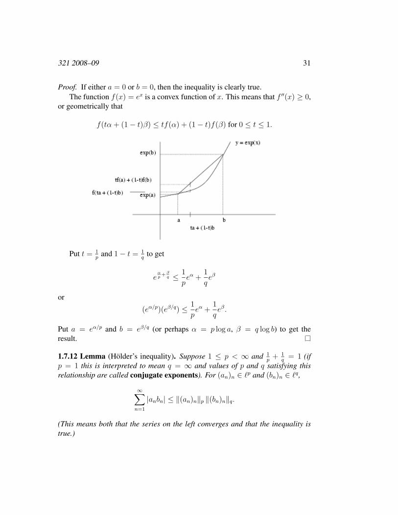
Proof. If either a = 0 or b = 0, then the inequality is clearly true.The function f(x) = ex is a convex function of x. This means that f ′′(x) ≥ 0,

or geometrically that

f(tα + (1− t)β) ≤ tf(α) + (1− t)f(β) for 0 ≤ t ≤ 1.

Put t = 1p

and 1− t = 1q

to get

eαp+β

q ≤ 1

peα +

1

qeβ

or

(eα/p)(eβ/q) ≤ 1

peα +

1

qeβ.

Put a = eα/p and b = eβ/q (or perhaps α = p log a, β = q log b) to get theresult.

1.7.12 Lemma (Holder’s inequality). Suppose 1 ≤ p < ∞ and 1p

+ 1q

= 1 (ifp = 1 this is interpreted to mean q = ∞ and values of p and q satisfying thisrelationship are called conjugate exponents). For (an)n ∈ `p and (bn)n ∈ `q,

∞∑n=1

|anbn| ≤ ‖(an)n‖p ‖(bn)n‖q.

(This means both that the series on the left converges and that the inequality istrue.)


Proof. This inequality is quite elementary if p = 1 and q = ∞. Suppose p > 1.Let

A = ‖(an)n‖p =

(∞∑

n=1

|an|p)1/p

B = ‖(bn)n‖q =

(∞∑

n=1

|bn|q)1/q

If either A = 0 or B = 0, the inequality is trivially true. Otherwise, useLemma 1.7.11 with a = |an|/A and b = |bn|/B to get

|anbn|AB

≤ 1

p

|an|p

Ap+

1

q

|bn|q

Bq

∞∑n=1

|anbn|AB

≤ 1

p

∑ |an|p

Ap+

1

q

∑ |bn|q

Bq

=1

p+

1

q= 1

Hence ∑|anbn| ≤ AB

1.7.13 Remark. For p = 2 and q = 2, Holder’s inequality reduces to an infinite-dimensional version of the Cauchy-Schwarz inequality

∞∑n=1

|anbn| ≤

(∑n

|an|2)1/2(∑

n

|yn|2)1/2

.

1.7.14 Lemma (Minkowski’s inequality). If x = (xn)n and y = (yn)n are in `p

(1 ≤ p ≤ ∞) then so is (xn + yn)n and

‖(xn + yn)n‖p ≤ ‖(xn)n‖p + ‖(yn)n‖p

Proof. This is quite trivial to prove for p = 1 and for p = ∞ (we have alreadyencountered the case p = ∞). So suppose 1 < p < ∞.

321 2008–09 33

First note that

|xn + yn| ≤ |xn|+ |yn| ≤ 2 max(|xn|, |yn|)|xn + yn|p ≤ 2p max(|xn|p, |yn|p)

≤ 2p(|xn|p + |yn|p

)∑

n

|xn + yn|p ≤ 2p(∑

n

|xn|p +∑

n

|yn|p)

This shows that (xn + yn)n ∈ `p.Next, to show the inequality,∑

n

|xn + yn|p =∑

n

|xn + yn| |xn + yn|p−1

=∑

n

|xn| |xn + yn|p−1 +∑

n

|yn| |xn + yn|p−1

Write∑

n |xn| |xn + yn|p−1 =∑

n anbn where an = |xn| and bn = |xn + yn|p−1.Then we have (an)n ∈ `p and (bn)n ∈ `q because∑

n

bqn =

∑n

|xn + yn|(p−1)q

=∑

n

|xn + yn|p < ∞

where we have used the relation 1p

+ 1q

= 1 to show (p − 1)q = p. FromLemma 1.7.12 we deduce

∑n

|xn||xn + yn|p−1 ≤

(∑n

|xn|p)1/p(∑

n

|xn + yn|(p−1)q

)1/q

= ‖(xn)n‖p‖(xn + yn)n‖p/qp

Similarly ∑n

|xn||xn + yn|p−1 ≤ ‖(yn)n‖p‖(xn + yn)n‖p/qp

Adding the two inequalities, we get

‖(xn + yn)n‖pp ≤ ‖(xn)n‖p‖(xn + yn)n‖p/q

p + ‖(yn)n‖p‖(xn + yn)n‖p/qp .


Now, if ‖(xn + yn)n‖p = 0 then the inequality to be proved is clearly satisfied. If‖(xn + yn)n‖p 6= 0, we can divide across by ‖(xn + yn)n‖p/q

p to obtain

‖(xn + yn)n‖p−p/qp ≤ ‖(xn)n‖p + ‖(yn)n‖p.

Since p− pq

= 1, this is the desired inequality.

Proof. (of Proposition 1.7.10): It follows easily from Lemma 1.7.14 that `p is avector space and that ‖ · ‖p is a norm on it (in fact Minkowski’s inequality is justthe triangle inequality for the `p-norm).

To show that `p is complete, we show that every absolutely convergent series∑k xk in `p is convergent. (That is we use Proposition 1.7.8.)Write xk = (xk,n)n = (xk,1, xk,2, . . .) for each k. Notice that

|xk,n| ≤ ‖xk‖p =

(∑n

|xk,n|p)1/p

Therefore∑

k |xk,n| ≤∑

k ‖xk‖p < ∞ for each k and it makes sense to write

yn =∑

k

xk,n

(and yn ∈ K).Now, for any N ≥ 1,(

N∑n=1

|yn|p)1/p

= limK→∞

(N∑

n=1

∣∣∣ K∑k=1

xk,n

∣∣∣p)1/p

= limK→∞

‖ ( x1,1, x1,2, . . . , x1,N , 0, 0, . . . )+ ( x2,1, x2,2, . . . , x2,N , 0, 0, . . . )...+ ( xK,1, xK,2, . . . , xK,N , 0, 0, . . . ) ‖p

≤ limK→∞

K∑k=1

‖(xk,1, xk,2, . . . , xk,N , 0, 0, . . .)‖p

(using Minkowski’s inequality)

321 2008–09 35

≤ limK→∞

K∑k=1

‖xk‖p

=∞∑

k=1

‖xk‖p < ∞

Letting N →∞, this shows that y = (yn)n ∈ `p.Applying similar reasoning to y−

∑K0

k=1 xk (for any given K0 ≥ 0) shows that∥∥∥∥∥y −K0∑k=1

xk

∥∥∥∥∥p

≤∞∑

K0+1

‖xk‖p

→ 0 as K0 →∞.

In other words the series∑

k xk converges to y in `p.

1.7.15 Examples. (i) We define, for 1 ≤ p < ∞,

Lp([0, 1]) = {f : [0, 1] → K : f measurable and∫ 1

0

|f(x)|p dx < ∞}.

On this space we define

‖f‖p =

(∫ 1

0

|f(x)|p dx

)1/p

The idea is that we have replaced sums used in `p by integrals over the unitinterval [0, 1]. It is perhaps natural to then allow measurable functions asthese are the right class to consider in the context of integration. One mightbe tempted to be more restrictive and (say) only allow continuous f but thiscauses problems we will mention later.

We can use the same ideas exactly as we used in the proofs of Holder’sinequality (Lemma 1.7.12) and Minkowski’s inequality (Lemma 1.7.14) toshow integral versions of them. We end up showing that

f, g ∈ Lp([0, 1]) ⇒ ‖f + g‖p ≤ ‖f‖p + ‖g‖p

(the triangle inequality). It is not at all hard to see that ‖λf‖p = |λ‖‖f‖p andwe are well on the way to showing ‖ · ‖p is a norm on Lp([0, 1]). However,it is not a norm. It is only a seminorm because ‖f‖p = 0 implies only that


{x ∈ [0, 1] : f(x) 6= 0} has measure 0 (total length 0). When somethingis true except for a set of total length 0 we say it is true almost everywhere[with respect to length measure or Lebesgue measure on R].

There is a standard way to get from a seminormed space to a normed space,by taking equivalence classes. We define an equivalence relation onLp([0, 1])by f ∼ g if ‖f−g‖p = 0 (which translates in this case to f(x) = g(x) almosteverywhere). We can then turn the set of equivalence classes

Lp([0, 1]) = {[f ] : f ∈ Lp([0, 1])}

into a vector space by defining

[f ] + [g] = [f + g], λ[f ] = [λf ].

There is quite a bit of checking to do to show this is well-defined. Anytimewe define operations on equivalence classes in terms of representatives ofthe equivalence classes, we have to show that the operation is independentof the choice of representatives.

Next we can define a norm on Lp([0, 1]) by ‖[f ]‖p = ‖f‖p (and again wehave to show this is well defined and actually leads to a norm). Finally weend up with a normed space (Lp([0, 1]), ‖ · ‖p) and it is in fact a Banachspace. The proof of that needs some facts from measure theory and can bebased on Proposition 1.7.8.

If∑∞

n=1 ‖fn‖p < ∞, let

g(x) = limN→∞

N∑n=1

|fn(x)| (x ∈ [0, 1])

with the understanding that g(x) ∈ [0, +∞]. By the monotone convergencetheorem ∫ 1

0

g(x)p dx = limN→∞

∫ 1

0

(N∑

n=1

|fn(x)|

)p

dx

From Minkowski’s inequality, we get(∫ 1

0

(N∑

n=1

|fn(x)|

)p

dx

)1/p

=

∥∥∥∥∥N∑

n=1

|fn|

∥∥∥∥∥p

≤N∑

n=1

‖|fn|‖p

=N∑

n=1

‖fn‖p ≤∞∑

n=1

‖fn‖p

321 2008–09 37

and it follows then that∫ 1

0

g(x)p dx ≤

(∞∑

n=1

‖fn‖p

)p

< ∞

and so g(x) < ∞ for almost every x ∈ [0, 1].

On the set where g(x) < ∞, we can define

f(x) =∞∑

n=1

fn(x) = limN→∞

N∑n=1

fn(x)

(and on the set of measure zero where g(x) = ∞ we can define f(x) = 0).Then f is measurable. From |f(x)| ≤ g(x) and the above, f ∈ Lp([0, 1]).To show limN→∞

∥∥∥(∑Nn=1 fn

)− f

∥∥∥p

= 0, use the fact that

∣∣∣∣∣(

N∑n=1

fn(x)

)− f(x)

∣∣∣∣∣ =

∣∣∣∣∣∞∑

n=N+1

fn(x)

∣∣∣∣∣ ≤ g(x)

(for almost every x ∈ [0, 1]). Since we know∫ 1

0g(x)p dx < ∞, the Lebesgue

dominated convergence theorem allows us to conclude

limN→∞

∥∥∥∥∥(

N∑n=1

fn

)− f

∥∥∥∥∥p

p

= limN→∞

∫ 1

0

∣∣∣∣∣(

N∑n=1

fn(x)

)− f(x)

∣∣∣∣∣p

dx

=

∫ 1

0

∣∣∣∣∣ limN→∞

(N∑

n=1

fn(x)

)− f(x)

∣∣∣∣∣p

dx = 0

Thus we have proved∑∞

n=1 fn converges to f in Lp([0, 1]).

We can never quite forget that Lp([0, 1]) is not actually a space of (measur-able) functions but really a space of (almost everywhere) equivalence classesof functions. However, it is usual not to dwell on this point. What it doesmean is that if you find yourself discussing f(1/2) or any specific singlevalue of f ∈ Lp([0, 1]), you are doing something wrong. The reason is thatas f ∈ Lp([0, 1]) is actually an equivalence class it is then possible to changethe value f(1/2) arbitrarily without changing the element of Lp([0, 1]) weare considering.


(ii) There are further variations on Lp([0, 1]) which are useful in different con-texts. We could replace [0, 1] by another interval [a, b] (a < b) and replace∫ 1

0by∫ b

a. For what we have discussed so far, everything will go through as

before. We get (Lp([a, b]), ‖ · ‖p).

(iii) We can also define Lp(R) where Lp(R) consists of measurable functionsf : R → K with

∫∞−∞ |f(x)|p dx < ∞. Then we take (as before) almost-

everywhere equivalence classes of f ∈ Lp(R) to be Lp(R) and we take thenorm ‖f‖p =

(∫R |f(x)|p dx

)1/p. Again we get a Banach space (Lp(R), ‖ ·‖p) for 1 ≤ p < ∞.

(iv) In fact we can define Lp in a more general context that includes all theexamples `p, Lp([a, b]) and Lp(R) as special cases. Let (X, Σ, µ) be ameasure space. This means X is a set, Σ is a collection of subsets ofX with certain properties, and µ is a function that assigns a measure (ormass or length or volume) in the range [0,∞] to each set in Σ. More pre-cisely Σ should be a σ-algebra of subsets of X — contains the empty setand X itself, closed under taking complements and countable unions. Andµ: Σ → [0,∞] should have µ(∅) = 0 and be countably additive (whichmeans that µ (

⋃∞n=1 En) =

∑∞n=1 µ(En) if E1, E2, . . . ∈ Σ are disjoint).

Then

Lp(X, Σ, µ) =

{f : X → K : f measurable,

∫X

|f(x)|p dµ(x) < ∞}

,

Lp(X, Σ, µ) consists of equivalence classes of elements inLp(X, Σ, µ) wheref ∼ g means that µ({x ∈ X : f(x) 6= g(x)}) = 0. We say that f = g almosteverywhere with respect to µ if f ∼ g (and sometimes write f = g a.e. [µ]).On Lp(X, Σ, µ) we take the norm

‖f‖p =

(∫X

|f(x)|p dµ(x)

)1/p

.

Then (Lp(X, Σ, µ), ‖ · ‖p) is a Banach space (1 ≤ p < ∞).

To see why the examples Lp([0, 1]), Lp([a, b]) and Lp(R) are special casesof Lp(X, Σ, µ) we take µ to be Lebesgue (length) measure on the line. Theneed for Σ is then significant — we cannot assign a length to every subsetof R and keep the countable additivity property. So Σ has to be Lebesgue-measurable subsets of [0, 1], [a, b] or R (or Borel measurable subsets). There

321 2008–09 39

is one reason why Lp([0, 1]) is a little different from the rest. In that casewe are dealing with a probability space (X, Σ, µ), meaning a measure spacewhere µ(X) = 1.

To see why `p is also an Lp(X, Σ, µ), we take X = N, Σ to be all subsetsof N and µ to be counting measure. This means that for E ⊂ N finite µ(E)is the number of elements in E and for E infinite, µ(E) = ∞. In this casewe can also think of functions f : N → K as sequences (f(n))∞n=1 of scalarsand

∫X|f(n)|p dµ(n) =

∑∞n=1 |f(n)|p for counting measure µ. Moreover,

the only set of measure 0 for counting measure is the empty set. Thus thereis no need to take almost everywhere equivalence classes when dealing withthis special case.

(v) We have avoided dealing with L∞ so far, because the formulae are slightlydifferent. Looking back to the comparison between `∞ and `p, we want toreplace the condition on the integral of |f |p being finite by a supremum. Wemight like to describe L∞(X, Σ, µ) as measurable f : X → K with

supx∈X

|f(x)| < ∞,

but in keeping with the case of Lp we also want to take a.e [µ] equivalenceclasses of such f . The problem is that while changing a function on a set ofmeasure 0 does not change its integral, it can change its supremum. Hencewe need a variation of the supremum that ignores sets of measure 0. This isknown as the essential supremum and it can be defined as

ess-sup(f) = inf

{sup

x∈X\E|f(x)| : E ⊂ X, µ(E) = 0

}or

ess-sup(f) = inf

{supx∈X

|g(x)| : g ∼ f

}(using g ∼ f to mean that g is a measurable function equal to f almosteverywhere). We then define

L∞(X, Σ, µ) = {f : X → K : f measurable, ess-sup(f) < ∞}

and L∞(X, Σ, µ) to be the almost everywhere equivalence classes of f ∈L∞(X, Σ, µ). With the norm

‖f‖∞ = ess-sup(f)


we get a Banach space (L∞(X, Σ, µ), ‖ · ‖∞).

In the case (X, Σ, µ) is X = N with counting measure, we can verify thatL∞ is just `∞ again. For X = [0, 1] we get L∞([0, 1]) (using µ = Lebesguemeasure) and we also have L∞([a, b]) and L∞(R).

Of course there are many details omitted here, to verify that everything is asclaimed, that the norms are well defined, that the spaces are complete, andso on.

(vi) We can further consider Lp (1 ≤ p ≤ ∞) in other cases, like Lp(Rn) wherewe take n-dimensional Lebesgue measure for µ (on X = Rn).

1.8 Linear operators1.8.1 Theorem. Let (E, ‖·‖E) and (F, ‖·‖F ) be normed spaces and let T : E → Fbe a linear transformation. Then the following are equivalent statements about T .

(i) T is continuous.

(ii) T is continuous at 0 ∈ E.

(iii) There exists M ≥ 0 so that ‖Tx‖F ≤ M‖x‖E holds for all x ∈ E.

(iv) T is a Lipschitz mapping, that is there exists M ≥ 0 so that ‖Tx− Ty‖F ≤M‖x− y‖E holds for all x, y ∈ E.

(v) T is uniformly continuous.

Proof. Our strategy for the proof is to show (i) ⇒ (ii) ⇒ (iii) ⇒ (iv) ⇒ (v) ⇒ (i).

(i) ⇒ (ii) Obvious

(ii) ⇒ (iii) By continuity at 0 (with ε = 1), there is δ > 0 so that

‖x‖E = ‖x− 0‖E < δ ⇒ ‖Tx− T0‖F = ‖Tx‖F < 1

Then for any y ∈ E with y 6= 0 we can take for example x = (δ/2)y/‖y‖E

to get ‖x‖ = δ/2 < δ and so conclude

‖Tx‖F =

∥∥∥∥T ( δ

2‖y‖E

y

)∥∥∥∥F

=

∥∥∥∥ δ

2‖y‖E

T (y)

∥∥∥∥F

=δ

2‖y‖E

‖Ty‖F < 1.

Thus ‖Ty‖F ≤ (2/δ)‖y‖E for all y ∈ E apart from y = 0. But for y = 0this inequality is also true and so we get (iii) with M = 2/δ > 0.

321 2008–09 41

(iii) ⇒ (iv) We have

‖Tx− Ty‖F = ‖T (x− y)‖F ≤ M‖x− y‖E

by linearity of T and (iii).

(iv) ⇒ (v) Given ε > 0, take δ = ε/(M + 1) > 0, then

‖x− y‖E < δ ⇒ ‖Tx− Ty‖F ≤ M‖x− y‖E < Mδ =εM

M + 1< ε.

Thus we have uniform continuity of T (see 1.4.10).

(v) ⇒ (i) Obvious (by Proposition 1.4.11).

1.8.2 Definition. We usually refer to a linear transformation T : E → F be-tween normed spaces that satisfies the condition (iii) of Theorem 1.8.1 above as abounded linear operator (or sometimes just as a linear operator).

1.8.3 Remark. From Theorem 1.8.1 we see that bounded is the same as continuousfor a linear operator between normed spaces. There are very few occasions infunctional analysis when we want to consider linear transformation that fail tobe continuous. At least that is so in the elementary theory. When we encounterdiscontinuous linear transformations in this course it will be in the context ofunpleasant phenomena or counterexamples.

1.8.4 Definition. If T : E → F is a bounded linear operator between normedspaces (E, ‖ · ‖E) and (F, ‖ · ‖F ), then we define the operator norm of T to be

‖T‖op = inf{M ≥ 0 : ‖Tx‖F ≤ M‖x‖E∀x ∈ E}

1.8.5 Proposition. If T : E → F is a bounded linear operator between normedspaces (E, ‖ · ‖E) and (F, ‖ · ‖F ), then

(a) ‖T‖op = inf{M ≥ 0 : ‖Tx − Ty‖F ≤ M‖x − y‖E∀x, y ∈ E} (thus ‖T‖op

is the smallest possible Lipschitz constant for T );

(b) ‖T‖op = sup{‖Tx‖F : x ∈ E, ‖x‖E = 1} (provided E 6= {0} or if weinterpret the right hand side as 0 in case we have the supremum of the emptyset);


(c) ‖T‖op = sup{‖Tx‖F : x ∈ E, ‖x‖E ≤ 1};

(d) ‖T‖op = sup{‖Tx‖F

‖x‖E: x ∈ E, x 6= 0

}(again provided E 6= {0} or if we

interpret the right hand side as 0 in case we have the supremum of the emptyset).

Proof. Exercise.

1.8.6 Examples. (i) We claim that if 1 ≤ p1 < p2 ≤ ∞, then `p1 ⊆ `p2 and theinclusion operator

T : `p1 → `p2

Tx = x

has ‖T‖op = 1.

Notice that this is nearly obvious for `1 ⊆ `∞ as∑∞

n=1 |xn| < ∞ implieslimn→∞ xn = 0 and so the sequence (xn)∞n=1 ∈ c0 ⊆ `∞.

In fact we can dispense with the case p2 = ∞ first because it is a littledifferent from the other cases. If (xn)∞n=1 ∈ `p1 , then

∑∞n=1 |xn|p < ∞

and so limn→∞ xn = 0. Thus, again, we have (xn)∞n=1 ∈ c0 ⊆ `∞. Wealso see that for any fixed m, |xm|p ≤

∑∞n=1 |xn|p = ‖(xn)∞n=1‖p1

p1and so

|xm| ≤ ‖x‖p1 for x = (xn)∞n=1. Thus

‖x‖∞ = supm|xm| ≤ ‖x‖p1

and this means ‖Tx‖∞ ≤ M‖x‖p1 with M = 1. So ‖T‖op ≤ 1. To show‖T‖op ≥ 1 consider the sequence (1, 0, 0, . . .) which has ‖Tx‖∞ = ‖x‖∞ =1 = ‖x‖p1 .

Now consider 1 ≤ p1 ≤ p2 < ∞. If x = (xn)∞n=1 ∈ `p1 and ‖x‖p1 ≤ 1, thenwe have

∞∑n=1

|xn|p1 = ‖x‖p1p1≤ 1

and so |xn| ≤ 1 for all n. It follows that

∞∑n=1

|xn|p2 =∞∑

n=1

|xn|p1|xn|p2−p1 ≤∞∑

n=1

|xn|p1 ≤ 1

321 2008–09 43

and so x ∈ `p2 (if ‖x‖p1 ≤ 1). For the remaining x ∈ `p1 with ‖x‖p1 ≥ 1, wehave y = x/‖x‖p1 of norm ‖y‖p1 = 1. Hence y ∈ `p2 and so x = ‖x‖p1y ∈`p2 . This shows `p1 ⊂ `p2 .

We saw above that ‖x‖p1 ≤ 1 ⇒ ‖Tx‖p2 = ‖x‖p2 ≤ 1 and this tells us‖T‖op ≤ 1. To show that the norm is not smaller than 1, consider the casex = (1, 0, 0, . . .) which has ‖Tx‖p2 = ‖x‖p2 = 1 = ‖x‖p1 .

(ii) If 1 ≤ p1 < p2 ≤ ∞, then Lp2([0, 1]) ⊆ Lp1([0, 1]) and the inclusionoperator

T : Lp2([0, 1]) → Lp1([0, 1])

Tf = f

has ‖T‖op = 1.

This means that the inclusions are in the reverse direction compared to theinclusions among `p spaces. One easy case is to see that L∞([0, 1]) ⊆L1([0, 1]) because ∫ 1

0

|f(x)| dx

will clearly be finite if the integrand is bounded.

The general case Lp2([0, 1]) ⊆ Lp1([0, 1]) (and the fact that the inclusionoperator has norm at most 1) follows from Holders inequality by taking oneof the functions to be the constant 1 and a suitable value of p. At least thisworks if p2 < ∞.

‖f‖p1p1

=

∫ 1

0

|f(x)|p1 dx

=

∫ 1

0

|f(x)|p11 dx

≤(∫ 1

0

(|f(x)|p1)p dx

)1/p(∫ 1

0

1q dx

)1/q

(with1

p+

1

q= 1)

=

(∫ 1

0

|f(x)|p1p dx

)1/p

= ‖f‖p1p1p


To make p1p = p2 we take p = p2/p1, which is allowed as p2 > p1. We get

‖f‖p1p1≤ ‖f‖p1

p2

and so we have ‖f‖p1 ≤ ‖f‖p2 .

If f ∈ Lp2([0, 1]), which means that ‖f‖p2 < ∞, we see that f ∈ Lp1([0, 1]).So we have inclusion as claimed, but also the inequality ‖f‖p1 ≤ ‖f‖p2 tellsus that ‖T‖op ≤ 1. Taking f to be the constant function 1, we see that‖f‖p1 = 1 = ‖f‖p2 and so ‖T‖op cannot be smaller than 1.

When p2 = ∞ there is a simpler argument based on∫ 1

0

|f(x)|p1 dx ≤∫ 1

0

‖f‖p1∞ dx = ‖f‖p1

∞

to show L∞([0, 1]) ⊆ Lp1([0, 1]) and the inclusion has norm at most 1.Again the constant function 1 shows that ‖T‖op = 1 in this case.

(iii) If (X, Σ, µ) is a finite measure space (that is if µ(X) < ∞) then we havea somewhat similar result to what we have for Lp([0, 1]). The inclusions gothe same way, but the inclusion operators can gave norm different from 1.If 1 ≤ p1 < p2 ≤ ∞, then Lp2(X, Σ, µ) ⊆ Lp1(X, Σ, µ) and the inclusionoperator

T : Lp2(X, Σ, µ) → Lp1(X, Σ, µ)

Tf = f

has‖T‖op = µ(X)(1/p1)−(1/p2).

The proof is quite similar to the previous case, but the difference comesfrom the fact that

∫X

1 dµ(x) = µ(X) and this is not necessarily 1. (Whenµ(X) = 1 we are in a probability space.) So when we use Holders in-equality, a constant will come out and the resulting estimate for ‖T‖op isthe value above. Again if you look at the constant function 1, you see that‖T‖op ≥ µ(X)(1/p1)−(1/p2).

(iv) When we look at the different Lp(R) spaces, we find that the argumentsabove don’t work. The argument with Holders inequality breaks down be-cause the constant function 1 has integral ∞ and the argument that workedfor `p does not go anywhere either.

321 2008–09 45

Looking at the extreme cases of p = 1 and p = ∞, there is no reason toconclude that |f(x)| bounded implies

∫∞−∞ |f(x)| dx should be finite. And

on the other hand functions where the integral is finite can be unbounded.

This actually turns out to be the case. We can find examples of function inLp1(R) but not in Lp2(R) for any values of 1 ≤ p1, p2 ≤ ∞ where p1 6= p2.

To see this we consider two examples of function fα, gα: R → K, given as

fα(x) =e−x2

|x|α, gα(x) =

1

1 + |x|α

(where α > 0).

When checking to see if fα ∈ Lp(R) (for p < ∞) or not we end up checkingif ∫ 1

0

1

xpαdx < ∞.

The reason is that∫∞−∞ |fα(x)|p dx = 2

∫∞0|fα(x)|p dx (even function) and

the e−x2 guarantees∫∞

1|fα(x)|p dx < ∞. In the range 0 < x < 1 the

exponential term is neither big nor small and does not affect convergence ofthe integral. The condition comes down to pα < 1 or α < 1/p. The casep = ∞ (and 1/p = 0) fits into this because (when α > 0) fα(x) → ∞ asx → 0 and so fα /∈ L∞(R).

For gα ∈ Lp(R) to hold we end up with the condition∫ ∞

1

1

xpαdx < ∞

(as gα(x) is within a constant factor of 1/xpα when x ≥ 1) which is true ifpα > 1 or α > 1/p.

Thus if 1 ≤ p1 < p2 ≤ ∞ and we choose α in the range

1

p2

< α <1

p1

we find

fα ∈ Lp1(R), fα /∈ Lp2(R), gα ∈ Lp2(R), gα /∈ Lp1(R),

which shows that neither Lp1(R) ⊆ Lp2(R) nor Lp2(R) ⊆ Lp1(R) is valid.


(v) You might wonder why in the case of (X, Σ, µ) being X = N with countingmeasure, and so µ(X) = ∞, we do get `p1 ⊆ `p2 but that this does not workwith X = R (where also µ(X) = ∞).

The difference can be explained by the fact that N is what is called as anatomic measure space. The singleton sets are of strictly positive measureand cannot be subdivided. On the other hand R is what is called ‘purelynonatomic’. There are no ‘atoms’ (sets of positive measure which cannot bewritten as the union of two disjoint parts each of positive measure).

1.8.7 Definition. Two normed spaces (E, ‖ · ‖E) and (F, ‖ · ‖F ) are isomorphicif there exists a vector space isomorphism T : E → F which is also a homeomor-phism.

We say that (E, ‖ · ‖E) and (F, ‖ · ‖F ) are called isometrically isomorphicif there exists a vector space isomorphism T : E → F which is also isometric(‖Tx‖F = ‖x‖E for all x ∈ E).

1.8.8 Remark. From Theorem 1.8.1, we can see that both T and T−1 are boundedif T : E → F is both a vector space isomorphism and a homeomorphism. Thusthere exist constants M1 = ‖T‖op and M2 = ‖T−1‖op so that

1

M2

‖x‖E ≤ ‖Tx‖F ≤ M1‖x‖E (∀x ∈ E)

This means that an isomorphism almost preserves distances (preserves them withinfixed ratios)

1

M2

‖x− y‖E ≤ ‖Tx− Ty‖F ≤ M1‖x− y‖E

as well as being a homeomorphism (which means more or less preserving thetopology).

Another way to think about it is that if we transfer the norm from F to E viathe map T to get a new norm on E given by

|||x||| = ‖Tx‖F

then we have1

M2

‖x‖E ≤ |||x||| ≤ M1‖x‖E.

1.8.9 Theorem. If (E, ‖ · ‖E) is a finite dimensional normed space of dimensionn, then E is isomorphic to Kn (with the standard Euclidean norm).

321 2008–09 47

Proof. Let v1, v2, . . . , vn be a vector space basis for E and define T : Kn → E by

T (x1, x2, . . . , xn) =n∑

i=1

xivi.

From standard linear algebra we know that T is a vector space isomorphism, andwhat we have to show is that T is also a homeomorphism.

To show first that T is continuous (or bounded) consider (for fixed 1 ≤ j ≤ n)the map Tj: Kn → E given by

Tj(x1, x2, . . . , xn) = xjvj.

We have ‖Tj(x)‖E = |xj|‖vj‖E ≤ ‖vj‖E‖x‖2 since ‖x‖2 = (∑n

i=1 |xi|2)1/2 ≥|xj|. From the triangle inequality we can deduce

‖Tx‖E =

∥∥∥∥∥n∑

j=1

Tj(x)

∥∥∥∥∥E

≤n∑

j=1

‖Tj(x)‖E ≤

(n∑

j=1

‖vj‖E

)‖x‖E

establishing that T is bounded (with operator norm at most∑n

j=1 ‖vj‖E).Now consider the unit sphere

S = {x ∈ Kn : ‖x‖2 = 1},

which we know to be a compact subset of Kn (as it is closed and bounded). SinceT is continuous, T (S) is a compact subset of E. Thus T (S) is closed in E (be-cause E is Hausdorff). Since T is bijective (and 0 /∈ S) we have 0 = T (0) /∈T (S). Thus there exists r > 0 so that

{y ∈ E : ‖y − 0‖E = ‖y‖E < r} ⊂ E \ S.

Another way to express this is

x ∈ Kn, ‖x‖2 = 1 ⇒ ‖Tx‖E ≥ r.

Scaling arbitrary x ∈ Kn \ {0} to get a unit vector x/‖x‖2 we find that∥∥∥∥T ( 1

‖x‖2

x

)∥∥∥∥E

=

∥∥∥∥ 1

‖x‖2

Tx

∥∥∥∥E

=1

‖x‖2

‖Tx‖E ≥ r

and so ‖Tx‖E ≥ r‖x‖2. This holds for x = 0 also. So for y ∈ E, we can takex = T−1y to get ‖y‖E ≥ r‖T−1y‖2, or

‖T−1y‖2 ≤1

r‖y‖E (∀y ∈ E).

Thus T−1 is bounded.


1.8.10 Corollary. If (E, ‖ · ‖E) is a finite dimensional normed space and T : E →F is any linear transformation with values in any normed space (F, ‖ · ‖F ), thenT is continuous.

Proof. Chose an isomorphism S: Kn → E (which exists by Theorem 1.8.9).Let e1, e2, . . . , en be the standard basis of Kn (so that e1 = (1, 0, . . . , 0), e2 =(0, 1, 0, . . . , o), etc.) and wi = (T ◦ S)(ei). Then

(T ◦ S)(x1, x2, . . . , xn) = (T ◦ S)

(n∑

i=1

xiei

)=

n∑i=1

xiwi

and as in the proof of Theorem 1.8.9 we can show that T ◦ S is bounded (in fact‖T ◦ S‖op ≤

∑ni=1 ‖wi‖F ). So T = (T ◦ S) ◦ S−1 is a composition of two

continuous linear operators, and is therefore continuous.

1.8.11 Example. The Corollary means that for finite dimensional normed spaces,continuity or boundedness of linear transformations is automatic. For that reasonwe concentrate most on infinite dimensional situations and we always restrict our(main) attention to bounded linear operators.

Although in finite dimensions boundedness is not in question, that only meansthat there exists some finite bound. There are still questions (which have beenconsidered in much detail by now in research) about what the best bounds are.These questions can be very difficult in finite dimensions. Part of the motivationfor this study is that a good understanding of the constants that arise in finitedimensions, and how they depend on increasing dimension, can reveal insightsabout infinite dimensional situations.

Consider the finite dimensional version of `p, that is Kn with the norm ‖ · ‖p

given by

‖(x1, x2, . . . , xn)‖p =

(n∑

i=1

|xi|p)1/p

for 1 ≤ p < ∞ and ‖(x1, x2, . . . , xn)‖∞ = max1≤i≤n |xi|. We denote this spaceby `p

n, with the n for dimension.Now, all the norms ‖ · ‖p are equivalent on Kn, that is given p1 and p2 there

are constants m, M > 0 so that

m‖x‖p1 ≤ ‖x‖p2 ≤ M‖x‖p1

holds for all x ∈ Kn. We can identify the constants more precisely. Say 1 ≤ p1 <p2 ≤ ∞. Then we know from the infinite dimensional inequality for `p spaces

321 2008–09 49

(applied to the finitely nonzero sequence (x1, x2, . . . , xn, 0, 0, . . .)) that ‖x‖p2 ≤‖x‖p1 .

We could also think of `pn as a Lp space where we take X = {1, 2, . . . , n}

with counting measure µ. From Examples 1.8.6 (iii) we know also ‖x‖p1 ≤n(1/p1)−(1/p2)‖x‖p2 . In summary

‖x‖p2 ≤ ‖x‖p1 ≤ n(1/p1)−(1/p2)‖x‖p2

One can visualise this geometrically (say in R2 to make things easy) in termsof the shapes of the open unit balls

B`pn

= {x ∈ `pn : ‖x‖p < 1}

The inequality above means

B`p1n⊆ B`

p2n⊆ n(1/p1)−(1/p2)B`

p1n

.

For p = 2 we get a familiar round ball or circular disc, but for other p theshapes are different. For p = 1 we get a diamond (or square) with corners (1, 0),(0, 1), (−1, 0) and (0,−1). This is because the unit ball is specified by |x1| +|x2| < 1. So in the positive quadrant this comes to x1 + x2 < 1, or (x1, x2) belowthe line joining (1, 0) and (0, 1).

The ball of (real) `∞2 on the other hand is given by max(|x1|, |x2|) < 1 or−1 ≤ xi ≤ 1. So its unit ball is a square with the 4 corners (±1,±1). Here is anattempt at drawing the unit balls for `2

2, `12 and `∞2 on the one picture.


For example the fact that

B`1n⊆ B`2n

⊆ n(1/1)−(1/2)B`1n=√

nB`1n

means for n = 2 that the diamond is contained in the circle and the circle iscontained in the diamond expanded by a factor

√2.

1.8.12 Corollary. Finite dimensional normed spaces are complete.

Proof. If E is an n-dimensional normed space, then there is an isomorphismT : Kn → E. As Kn is complete and T−1 is uniformly continuous, it followsfrom Proposition 1.4.16 that E is complete.

1.9 Open mapping, closed graph and uniform boundedness the-orems

1.9.1 Theorem (Open Mapping Theorem). Let (E, ‖ · ‖E) and (F, ‖ · ‖F ) beBanach spaces and T : E → F a surjective bounded linear operator. Then thereexists δ > 0 so that

T (BE) ⊇ δBF

where BE = {x ∈ E : ‖x‖E < 1} and BF = {y ∈ F : ‖y‖F < 1} are the openunit balls of E and F .

Moreover, if U ⊆ E is open, then T (U) is open (in F ).

Proof. First we show that the second statement (the ‘open mapping’ part) followsfrom the first.

It is handy to note that all (open) balls B(x0, r) = {x ∈ E : ‖x−x0‖E < r} ina normed space (or Banach space) E can be related to the unit ball BE as follows

B(x0, r) = x0 + rBE

(where rBE = {rx : x ∈ BE} is a stretching of BE be the factor r and x0+rBE ={x0 + rx : x ∈ BE} is the translate of rBE by x0).

So if U ⊆ E is open and y0 ∈ T (U) then we know y0 = T (x0) for somex0 ∈ U . Since U is open, there is r > 0 with x0 + rBE = B(x0, r) ⊆ U . Itfollows from T (BE) ⊇ δBF and linearity of T that

T (U) ⊇ T (x0 + rBE) = T (x0) + rT (BE) ⊇ y0 + rδBF = B(y0, rδ).

321 2008–09 51

Thus y0 is an interior point of T (U). As this is true of all y0 ∈ T (U), we haveshown that T (U) is open.

Now to prove the first assertion, let Vr = T (rBE) = rT (BE) for r > 0.Because T is surjective and E =

⋃∞n=1 nBE , we have

F =∞⋃

n=1

T (nBE) =∞⋃

n=1

Vn.

By the Baire category theorem (and this is where we use the assumption that F iscomplete) we cannot have Vn nowhere dense for all n. (See §1.6 for an explanationof what the Baire category theorem says, and its proof.) That means there is n sothat the closure Vn has nonempty interior, or in other words there is y0 ∈ Vn andr > 0 with B(y0, r) = y0 + rBF ⊆ Vn.

By changing y0 and reducing r we can assume y0 ∈ Vn (and not just y0

in the closure). The idea is that there must be y1 ∈ Vn ∩ B(y0, r/2) and thenB(y1, r/2) ⊆ B(y0, r) ⊆ Vn. Write y1 = T (x0) for x0 ∈ nBE . Then we claimthat V2n ⊇ (r/2)BF . The argument is that x0 ∈ nBE implies

2nBE ⊇ nBE − x0

and soV2n ⊇ T (nBE − x0) = T (nBE)− T (x0) = Vn − y1

Taking closures, we get

V2n ⊇ Vn − y1 ⊇ (y1 + (r/2)BF )− y1 = (r/2)BF .

The fact that the closure of Vn − y1 is the same as Vn − y1 follows from thefact that the translation map y 7→ y − y1: F → F is distance preserving (and soa homeomorphism) of F onto itself (with inverse the translation y 7→ y + y1).Homeomorphisms preserve all topological things, and map closures to closures.

For k ∈ N we have Vkn = (kVn) = kVn (one can check that because y 7→ kyis a homeomorphism with inverse y 7→ (1/k)y). Thus, if k big enough so thatkr/2 > 1 we have

Vkn = kVn ⊇ kr

2BF ⊇ BF

Let N = kn. Thus we have VN ⊇ BF . What we claim is that V3N ⊇ BF (noclosure now on the V3N ).


From VN ⊇ BF we deduce, for j ∈ N,

VN/j =1

jVN =

1

jVN ⊇ 1

jBF

Starting with any y ∈ BF we must have x1 ∈ NBE (so T (x1) ∈ VN ) with

‖y − T (x1)‖F <1

2

ory − T (x1) ∈

1

2BF ⊆ VN/2.

We can then find x2 ∈ (N/2)BE (so T (x2) ∈ VN/2) with

‖(y − T (x1))− T (x2)‖F <1

22

ory − T (x1)− T (x2) = y − (T (x1) + T (x2)) ∈

1

22BF ⊆ VN/22 .

By induction, we can find x1, x2, . . . with xj ∈ (N/2j−1)BE and

y −j∑

i=1

T (xi) ∈1

2jBF ⊆ VN/2j .

With this construction we have an absolutely convergent series∑∞

j=1 xj in E,because

∞∑j=1

‖xj‖E ≤∞∑

j=1

N

2j−1= 2N < 3N.

Now using completeness of E (remember we used completeness of F earlier) weknow from Proposition 1.7.8 that

∑∞j=1 xj converges in E. That says there is

x ∈ E with x = limj→∞∑j

i=1 xi and in fact we know

‖x‖E ≤ limj→∞

∥∥∥∥∥j∑

i=1

xi

∥∥∥∥∥E

≤ limj→∞

j∑i=1

‖xi‖E ≤ 2N < 3N

because the closed ball B(0, 2N) is closed in E and all the partial sums∑j

i=1 xi

are inside B(0, 2N).

321 2008–09 53

As T is linear and continuous, we also have

Tx = limj→∞

T

(j∑

i=1

xi

)= lim

j→∞

j∑i=1

T (xi) = y

because ∥∥∥∥∥y −j∑

i=1

T (xi)

∥∥∥∥∥F

≤ 1

2j→ 0

as j →∞.So we have y = T (x) ∈ V3N = T (3NBE). Since this is so for all y ∈ BF , we

have BF ⊆ V3N as claimed. It follows that

T (BE) ⊆ 1

3NBF ,

which is the result with δ = 1/(3N) > 0.

1.9.2 Corollary. If E, F are Banach spaces and T : E → F is a bounded linearoperator that is also bijective, then T is an isomorphism.

Proof. By the Open Mapping theorem T is automatically an open map, that isU ⊆ E open implies T (U) ⊆ F open. But, since T is a bijection the forwardimage T (U) is the same as the inverse image (T−1)−1(U) of U under the inversemap T−1.

Thus the open mapping condition says that T−1 is continuous.

1.9.3 Theorem (Closed graph theorem). If E, F are Banach spaces and T : E →F is a linear transformation, then T is bounded if and only if its ‘graph’

{(x, y) ∈ E × F : y = Tx}

is a closed subset of E × F in the product topology.

Proof. It is quite easy to check that the graph must be closed if T is bounded(continuous). The product topology is a metric space topology as E and F aremetric spaces, and in fact arises from a norm on E⊕F . (See §A.2 and §A.3.) Fordefiniteness we take the norm

‖(x, y)‖1 = ‖x‖+ ‖y‖


on E ⊕ F , or we could write E ⊕1 F . So to show the graph is closed, supposewe have a sequence (xn, yn) in the graph that converges in E × F to some limit(x, y). We claim that (x, y) must be in the graph, that is that y = Tx.

What we know is that yn = Txn for each n (since (xn, yn) is in the graph).As (xn, yn) → (x, y) in the product topology, it follows that xn → x and yn → y(as n → ∞). (This is rather easy as ‖xn − x‖ ≤ ‖(xn, yn) − (x, y)‖1 = ‖(xn −x, yn − y)‖n → 0 as n →∞.) But T is continuous and so T (xn) → T (x). SinceT (xn) = yn, that means yn → T (x). As yn → y also (because ‖yn − y‖ ≤‖(xn, yn) − (x, y)‖1) and in metric spaces sequences can have at most one limit,we have T (x) = y and (x, y) is in the graph — as we wanted to show.

Now assume that the graph is closed. Our proof that T must be continuousrelies on the open mapping theorem. We introduce a new norm on E by

|||x||| = ‖x‖E + ‖Tx‖F .

It is not at all difficult to check that this is indeed a norm:

|||x1 + x2||| = ‖x1 + x2‖E + ‖T (x1 + x2)‖F

= ‖x1 + x2‖E + ‖T (x1) + T (x2)‖F

≤ ‖x1‖E + ‖x2‖E + ‖T (x1)‖F + ‖T (x2)‖F

= |||x1|||+ |||x2||||||λx||| = ‖λx‖E + ‖T (λx)‖F

= ‖λx‖E + ‖λTx‖F

= |λ|‖x‖E + |λ|‖Tx‖F

= |λ||||x||||||x||| = 0 ⇒ ‖x‖E = 0

⇒ x = 0

We consider the identity mapping id: (E, ||| · |||) → (E, ‖ · ‖E) which is clearlylinear, bijective and bounded since

‖id(x)‖E = ‖x‖E ≤ |||x|||.

In order to apply the open mapping theorem we need to know that (E, ||| · |||) isa Banach space (that is complete) and in doing that the hypothesis that the graphis closed will be used. Once we have verified completeness, the open mappingtheorem guarantees that the inverse map id−1: (E, ‖·‖E) → (E, |||·|||) is continuous.Therefore its is bounded, or there exists M ≥ 0 so that

|||x||| ≤ M‖x‖E

321 2008–09 55

holds for all x ∈ E. That implies ‖Tx‖F ≤ |||x||| ≤ M‖x‖E and so T bounded aswe need.

It remains to verify the completeness of (E, ||| · |||). Take a Cauchy sequence(xn)∞n=1 in E with respect to the metric arising from ||| · |||. Then for ε > 0 givenand n, m large enough

|||xn − xm||| < ε.

But that implies both ‖xn − xm‖E < ε and ‖T (xn)− T (xm)‖F < ε. This means(xn)∞n=1 is a Cauchy sequence in (E, ‖ ·‖E) and (T (xn))∞n=1 is a Cauchy sequencein (F, ‖ · ‖F ). As both E and F are complete there exists x = limn→∞ xn ∈ Eand y = limn→∞ T (xn) ∈ F . Using 3.39 (ii) we see that

(xn, T (xn)) → (x, y)

in the product topology of E × F . But each (xn, T (xn)) is in the graph of T andwe are assuming that the graph is closed. So the limit (x, y) is also in the graph,or y = Tx. It follows that

limn→∞

|||xn−x||| = limn→∞

‖xn−x‖E+‖T (xn)−Tx‖F = limn→∞

‖xn−x‖E+‖yn−y‖F = 0

and that means xn → x in (E, ||| · |||). WE have shown that each Cauchy sequencein (E, ||| · |||) converges. So (E, ||| · |||) is complete.

As noted above, the result follows then from the open mapping theorem.

1.9.4 Theorem (Uniform boundedness principle). Let E be a Banach space andF a normed space. Let Ti: E → F be bounded linear operators for i ∈ I = someindex set. Assume

supi∈I

‖Ti(x)‖ < ∞ for each x ∈ E

(which can be stated as the family of operators being pointwise uniformly bounded).Then

supi∈I

‖Ti‖ < ∞

(uniform boundedness in norm).

Proof. The proof relies on the Baire category theorem in E.Let

Wn = {x ∈ E : supi∈I

‖Tix‖ ≤ n}

=⋂i∈I

{x ∈ E : ‖Tix‖ ≤ n}.


Then Wn is closed as it is the intersection of closed sets. ({x ∈ E : ‖Tix‖ ≤ n}is the inverse image under Ti of the closed ball {y ∈ F : ‖y‖ ≤ n}, and Ti iscontinuous. So the inverse image is closed.)

The hypothesis implies that each x ∈ E belongs in Wn for some n, or that⋃∞n=1 Wn = E. By the Baire category theorem, there is some n where Wn is not

nowhere dense. Fix this n. As Wn is closed, Wn not nowhere dense means thatWn has nonempty interior. So there is x0 and r > 0 so that

B(x0, r) = x0 + rBE ⊆ Wn.

Thus‖Ti(x0 + rx)‖ = ‖Ti(x0) + rTi(x)‖ ≤ n

holds for all x ∈ BE . It follows that

r‖Ti(x)‖ − ‖Ti(x0)‖ ≤ n (∀x ∈ BE)

and so‖Ti(x)‖ ≤ 1

r‖Ti(x0)‖+

n

r≤ 2n

r(∀x ∈ BE)

since x0 ∈ Wn ⇒ ‖Ti(x0)‖ ≤ n for all i ∈ I . Take supx∈BEto get

‖Ti‖ ≤2n

r

and as this is true for each i ∈ I , we have supi∈I ‖Ti‖ ≤ 2n/r < ∞ as required.

1.9.5 Remark. The open mapping, closed graph and uniform boundedness princi-ple are all considered to be fundamental theorems in functional analysis. We willpostpone giving examples of their use until we discuss Fourier series later.

There is at least one more theorem of central importance, the Hahn Banachtheorem, and again we leave that for a while.

321 2008–09 i

A Appendix

A.1 Uniform convergenceWe recall here some facts about unform convergence of sequences of functions(with values in a metric space).

A.1.1 Definition. Let X be a topological space and (Y, d) a metric space. Letfn: X → Y be functions (n = 1, 2, 3, . . .) and f0: X → Y another function.

Then we say that the sequence (fn)∞n=1 converges uniformly on X to f0 if thefollowing is true

for each ε > 0 there exists N > 0 so that

n ≥ N, x ∈ X ⇒ d(fn(x), f0(x)) < ε.

A.1.2 Proposition. (‘uniform limits of continuous functions are continuous’) LetX be a topological space and (Y, d) a metric space. If (fn)∞n=1 is a sequence ofcontinuous functions fn: X → Y that converges uniformly on X to f0: X → Y ,then f0 is continuous.

Proof. Fix x0 ∈ X and our aim will be to show that f is continuous at x0. So takea neighbourhood NY of y0 = f(x0) ∈ Y , and our aim is to show f−1(NY ) is aneighbourhood of x0 ∈ X .

There is ε > 0 so that B(y0, ε) ⊆ NY . By uniform convergence we can findn0 so that

n ≥ n0, x ∈ X ⇒ d(fn(x), f(x)) <ε

3.

Fix n = n0. By continuity of fn at x0,

NX = f−1n

(B(fn(x0),

ε

3

)={

x ∈ X : d(fn(x), fn(x0)) <ε

3

}is a neighbourhood of x0 ∈ X . For x ∈ NX we have

d(f(x), f(x0)) ≤ d(f(x), fn(x)) + d(fn(x), fn(x0)) + d(fn(x0), f(x0))

<ε

3+

ε

3+

ε

3= ε

This implies f(x) ∈ B(f(x0), ε) ⊆ NY ∀x ∈ NX or that NX ⊆ f−1(NY ). Sof−1(NY ) is a neighbourhood of x0 ∈ X .

This shows f continuous at x0 ∈ X . As x0 is arbitrary, f is continuous.

ii Chapter 1: Banach Spaces

A.2 Products of two metric spacesGiven two metric space (X, dX) and (Y, dY ), we can make the cartesian productX × Y = {(x, y) : x ∈ X, y ∈ Y } into a metric space in a number of ways. Forexample we can define a metric

d∞ on X × Y by the rule

d∞((x1, y1), (x2, y2)) = max(dX(x1, x2), dY (y1, y2)).

It is not very difficult to check that his does define a metric. For example thetriangle inequality

d∞((x1, y1), (x3, y3)) ≤ d∞((x1, y1), (x2, y2)) + d∞((x2, y2), (x3, y3)),

we start by

d∞((x1, y1), (x3, y3)) = max(dX(x1, x3), dY (y1, y3))

≤ max(dX(x1, x2) + dX(x2, x3), dY (y1, y2) + dX(y2, y3))

(since dX(x1, x3) ≤ dX(x1, x2) + dX(x2, x3) and dY (y1, y3) ≤ dY (y1, y2) +dX(y2, y3) by the triangle inequalities for dX and Dy). Then use the triangle in-equality for the norm ‖ · ‖∞ on R2.

However, the most familiar example of a product is perhaps R2 = R × Rand the familiar Euclidean metric on R2 is not the one we get by using d∞ withdR(x1, x2) = dX(x1, x2) = |x1 − x2|, dY = dX . Motivated by that example, wemight prefer to think of a different metric d2 on the product of two metric spaces(X, dX) and (Y, dY ) where we take

d2((x1, y1), (x2, y2)) =√

(dX(x1, x2))2 + (dY (y1, y2))2 = ‖(dX(x1, x2), dY (y1, y2))‖2.

The proof that d2 is a metric is not that different from the proof that d∞ is a metricon X × Y .

More generally we might take p in the range 1 ≤ p < ∞ and define dp onX × Y by

dp((x1, y1), (x2, y2)) = ((dX(x1, x2))p + (dY (y1, y2))

p)1/p = ‖(dX(x1, x2), dY (y1, y2))‖p.

Again it is not that hard to show that dp is a metric.We have now an embarrassment of definitions in that we have infinitely many

choices (X × Y, dp) with 1 ≤ p ≤ ∞. However, all these metrics are somewhatcomparable because if 1 ≤ p1 ≤ p2 ≤ ∞, then

‖a‖p2 ≤ ‖a‖p1 ≤ 2‖a‖p2 (a ∈ R2)

321 2008–09 iii

(see Example 1.8.11 with n = 2, where a more precise constant is given). Itfollows that

dp2((x1, y1), (x2, y2)) ≤ dp1((x1, y1), (x2, y2)) ≤ 2dp2((x1, y1), (x2, y2))

and as a consequence the open sets in (X × Y, dp) are the same for every p. Sothe continuous functions with domains X × Y and values in some topologicalspace Z are the same no matter what matric we use. The same is true of functionsf : Z → X × Y with values in X × Y . Moreover the sequences ((xn, yn))∞n=1 thatconverge in (X × Y, dp) do not depend on the value of p we use.

It is possible to describe the topology on X × Y arising from any one of thesemetrics dp in a way that uses only topology (open sets). We will not do that at thisstage. The topology on X×Y arising from any one of the dp is called the producttopology.

A.3 Direct sum of two normed spacesIf we start with normed spaces (E, ‖·‖E) and (F, ‖·‖F ), then we can make E×Finto a vector space by defining vector space operations as follows:

(x1, y1) + (x2, y2) = (x1 + x2, y1 + y2) (for (x1, y1), (x2, y2) ∈ E × F )

λ(x, y) = (λx, λy) (for λ ∈ K, (x, y) ∈ E × F ).

One can check in a straightforward way that this make E ×F into a vector space,and the usual notation for this is E ⊕ F (called the direct sum of E and F ).

Inside E ⊕ F there is a subspace

E ⊕ {0} = {(x, 0) : x ∈ E}

that behaves just like E (is isomorphic as a vector space to E) and another sub-space {0} ⊕ F = {(0, y) : y ∈ F} that is a copy of F . Every (x, y) ∈ E ⊕ F canbe expressed in a unique way as

(x, y) = (x, 0) + (0, y)

as a sum of an element of E ⊕ {0} and an element of {0} ⊕ F .So far this is about vector spaces and so belongs to linear algebra. To make

E ⊕ F a normed space, we have at least the same sort of choices for norms as we

iv Chapter 1: Banach Spaces

discussed for metrics in a product metric space. For 1 ≤ p ≤ ∞ we can define anorm on E ⊕ F by

‖(x, y)‖p = ‖(‖x‖E, ‖y‖F )‖p = (‖x‖pE + ‖y‖p

F )1/p

(in terms of the p-norm of R2). It is not hard to check that this is a norm and thatthe distance arising from this norm is the same as the metric dp arising from themetrics dE and dF given by the norms on E and F .

It is common to write E ⊕p F for E ⊕ F with the norm ‖ · ‖p.

Richard M. Timoney (January 18, 2009)

Documents

Chapter 1: Banach Spaces - School of Mathematicsrichardt/321/321-ch1.pdf · Chapter 1: Banach Spaces Themainmotivationforfunctionalanalysiswasprobablythedesiretounderstand solutions