Embed Size (px)
Citation preview

ESI Software Demonstration Guide Page: 1
Groundwater Vistas Tutorial
Thank you for taking the time to try out our groundwater modeling software. Hopefully you will see how easy itis to create groundwater models in Windows using Groundwater Vistas. We recognize, however, that there is alot of competition in the environmental industry for such software and we also know that there are other factorsinvolved in your purchasing decision. Here are some factors we think may be important to you that set us apartfrom our competition:
Windows! We are committed to Microsoft Windows at every level. We are members of the MicrosoftDeveloper Network and our software supports all versions of Windows from 3.1 through the new NT 4.0. Forthose of you still clinging to DOS, you should get used to the idea of Windows because Microsoft will no longersupport DOS as you know it after the release of NT 4.0 this fall.
Support! One of the most important aspects of your purchase is the need for solid technical support from thesoftware developer and excellent free and unlimited technical support is provided. Not only will we answeryour questions related to the mechanics of using the software, but we will also help you with your project. Mostenvironmental software companies limit support to running the software and will not venture into consulting.We are groundwater modeling consultants as well as software developers and will try to help you no matterwhat the question.
Updates! Most updates from are free and are distributed via Internet. These updates can be sent to you viaemail, Internet ftp, or through the mail. If you find a bug in the software, we will fix it immediately (usually thesame day) and make it available to you on Internet as soon as the problem is fixed. If you do not have Internetaccess, we will send the repaired code to you via Federal Express at our expense.
Price! Our software is less expensive than most of our competition. We are also extremely competitive forvolume discounts. Call 703-620-9214 to negotiate a multi-user license!
Training! We provide numerous on-site training courses to government and private industry each year. Theseseminars are hands-on courses in applied groundwater modeling using this software. On-site training is a verycost-effective way of providing professional development opportunities for your staff. For the cost of sendingone or two staff to an outside short course, you can train a dozen or more staff in-house. Call for moreinformation and a proposal to provide your organization with training in groundwater modeling.
I hope that we will have an opportunity to work with you on your groundwater modeling projects. If you haveany questions regarding this software, support, consulting, or training, please do not hesitate to call or email to:
Scientific Software GroupP.O. Box 23041Washington, DC 20026-3041Phone: (703) 620-9214Fax: (703) 620-6793

ESI Software Demonstration Guide Page: 2
Welcome to the Groundwater Software Demos!Thank you for your interest in Groundwater Vistas. This guide shows you how to install, explore, and uninstall demonstration versions ofthe following products:
Groundwater Vistas, a comprehensive modeling environment for Windows, Page 4MODFLOWwin32, version of the popular MODFLOW3D groundwater flow model, Page 15WinFlow, a 2D analytic element groundwater flow model, and Page 20WinTran, a 2D analytic element flow model coupled with a finite-element transport model. Page 25
All of the demos are installed from one set of disks, as explained in the following section. After installing any or all demos, turn to thepage listed above for a particular demo and follow the instructions to find out more about the software. Each demo is a fully functioningversion of the software except that files cannot be saved and printing has been disabled. The last page of this guide contains an order formif you wish to purchase any of the software packages. If you have any questions as you are working through this guide, please do nothesitate to call us.
Contents and InstallationThe demos come with a sophisticated installation program that is similar to other Windows products. You simply run “install” fromthe Program Manager File menu and follow the directions as the installation proceeds. Start by placing the first demo disk in drive A:(or B:). Now, select Run from the File menu in Program Manager (the Start menu in Windows 95) and enter the following:
a:install.exe <� �
You will first be prompted for the directory that will contain all of the demo software. The default is c:\esidemos. Next, select theProgram Manager group that will contain the ESI icons. The default selection is “ESI Demos”. Finally, you will be given the optionof installing each demo, starting with MODFLOWwin32. (NOTE: you must install MODFLOWwin32 if you intend to useGroundwater Vistas!) When the installation program prompts for a particular demo, simply select Yes to install that demo or No tomove to the next software package. Select CANCEL at any time to terminate the installation process. The installation program willnow copy all of the MODFLOWwin32 files into the directory you entered above. Next, the readme text file will be displayed to alertyou to new information that was not available when the manual was created. Select OK when you are done reading the information.Although MODFLOWwin32 was used in this explanation, all of the demos are installed with the same sequence of prompts.
If you have installed any of the demos, a dialog box will ask you to modify the autoexec.bat file on your computer. ESI Demos requirethat the environment variable TMP be set so that temporary files can be properly maintained. Modifying the autoexec.bat file herewill properly set the TMP variable. Select YES to automatically make this change now or NO to change it yourself. If you do not setthe TMP environment variable, the demos will not run. In this case, double-clicking on any of the demo icons displays a dialog askingyou to set the TMP variable before the program can be executed. To set the TMP environment variable yourself, add the followingline to your autoexec.bat file
set TMP=c:\tmp
(Note: you will receive an error message that says “The DOS environment variable TMP must be set to a valid directory” ifyou do not place the above line in your autoexec.bat file) Finally, a dialog box appears telling you to restart your computer tocomplete the installation. Please note, however, that this dialog only appears when you have changed the autoexec.bat file as discussedabove. It will also not appear if you install Win32s below.
Installing Win32sGroundwater Vistas, MODFLOWwin32 and WinTran demonstration programs also need Microsoft’s Win32s software. Thisallows Windows V3.1 and V3.11 to run 32-bit software like MODFLOWwin32. If you are running Windows 95 or Windows NT, skipthis step.
Installing Win32s will not harm your system in any way! In fact, it is only used if you run 32-bit applications. After you are done withthe demonstration versions of ESI Software, you may delete it from your system, as described in the next section. In order to make iteasier to get rid of Win32s, we suggest that you make a backup copy of your SYSTEM.INI file, located in your c:\windows directory.If you plan to purchase either Groundwater Vistas, MODFLOWwin32 or WinTran, you may want to just leave Win32s on your system,as you will need it for these applications.

ESI Software Demonstration Guide Page: 3
The Win32s installation is straightforward. If you have installed demos for Groundwater Vistas, MODFLOWwin32 or WinTran, theinstallation program will ask you to install Win32s. Simply select Yes to install Win32s. Again, if you are running Windows 95 orNT, the installation program will not prompt you to install Win32s. If you are running Windows 95 or NT and you receive thisprompt, then you made an error in selecting the operating system at the beginning of the installation. You should reinstall the softwarebefore continuing with the demonstrations.
Follow the prompts to install the Win32s software. After the installation is complete, you will be asked to restart Windows. You mustdo this in order to run the demos. After restarting Windows, you must exit from Windows and reboot your computer so that theTMP environment variable will take effect.
Uninstalling Demos
These demos come with an uninstallation program to make it easy to remove the software from your computer when you are done withyour evaluation. To do so, simply double-click on the uninstall icon for the demo you wish to uninstall. You have 3 choices: (1)select automatic to quickly remove all of the demo files, (2) select custom to determine which files will be deleted, or (3) select cancelto end the uninstall program.
The uninstall program will not harm any program or file in your Windows directory or any other directory. Only files placed on yourcomputer related to ESI demos will be removed. If you do not wish to use the uninstall program, simply delete the contents of thedirectory containing the demo software and delete the “ESI Demos” Program Manager Group in Windows.
Uninstalling Win32s
Unfortunately, Microsoft does not provide an uninstall program for Win32s; however, the process is fairly simple. This is especiallytrue if you made a backup copy of your SYSTEM.INI file in the C:\WINDOWS directory. Follow these steps to remove Win32s fromyour computer:
If you made a backup copy of SYSTEM.INI and you have not installed any other software since installing the GV, MODFLOWwin32
or WinTran demos, copy the old version of SYSTEM.INI back to your Windows directory (usually C:\WINDOWS) and skip to step 3below.
(1) Remove the following line from the [386Enh] section in the SYSTEM.INI file:
device=<WINDOWS>\<SYSTEM>\win32s\w32s.386
where <Windows> and <System> are where the Windows and System directories are, respectively. This is usuallyC:\WINDOWS\SYSTEM.
(2) Modify the following line from the [BOOT] section in the SYSTEM.INI file:
drivers=mmsystem.dll winmm16.dll
to the following (remove winmm16.dll):
drivers=mmsystem.dll
(3) Delete the following files from the <WINDOWS>\<SYSTEM> subdirectory or from the SYSTEM directory in networkinstallations:
W32SYS.DLL WIN32S16.DLL WIN32S.INI
(4) Delete all the files in the <WINDOWS>\<SYSTEM>\WIN32S subdirectory or the <SYSTEM>\WIN32S subdirectory in networkinstallations. Then, delete the WIN32S subdirectory itself.
(5) Restart Windows

ESI Software Demonstration Guide Page: 4
Groundwater Vistas (GV) Demo!Groundwater Vistas is Environmental Simulations’s newgroundwater modeling environment for MicrosoftWindows. Groundwater Vistas, or GV, is compatiblewith ModelCad386 from Geraghty & Miller because bothprograms were written by the same author. However,GV goes beyond the capabilities of ModelCad or anyother model preprocessor. GV is designed to be a cost-effective alternative to more expensive programs, suchas ModelCad, Visual MODFLOW, MODIME, PMWINand GMS. The following are the unique features of GVthat set it apart from other preprocessors:
(1) Groundwater Vistas is designed specifically forWindows 3.1, Windows 95, and Windows NT(including the new Windows NT V4.0). The userinterface follows Microsoft’s conventions makingthe software easy to learn. The entire User’sManual is included as on-line, context-sensitivehelp.
(2) Groundwater Vistas is model-independent,supporting several different models including
MODFLOW,MT3D,PATH3D,MODPATH,MODFLOWT (a new transport mode),MODFLOW-SURFACT (a new version of MODFLOW), andPEST, the model-independent calibration software.FTWORK, MODFLOWP, SUTRA and BIOPLUME II are also planned for the next release.
(3) Groundwater Vistas provides visualization of output from all supported models. This includes contouring, color flood contouring,velocity vectors, particle-trace display, and a detailed mass-balance analyzer (not found in the other competitors). All graphics aredisplayed in plan view and in cross-section at the same time using a split window. GV also plots head, drawdown, andconcentration versus time at observationpoints, parameter sensitivity graphs, andprofiles of head, concentration, drawdown,or flux along a cross-section.
(4) Boundary conditions may be specified eitheron a cell-by-cell basis or using grid-independent locations. The latter allows youto modify the grid without influencing thelocation of boundaries.

ESI Software Demonstration Guide Page: 5
Groundwater VistasAdvanced Model Design & Analysis for Windows!
Groundwater Vistas (GV) is a unique groundwatermodeling environment for Microsoft Windows thatcouples a powerful model design system withcomprehensive graphical analysis tools. GV, developedby the author of ModelCadTM, is a model-independentgraphical design system for MODFLOW and relatedmodels. In addition, GV supports the use of the PESTmodel-independent calibration software. Thecombination of PEST (a trial version is included withGV) and GV’s automatic sensitivity analysis make GV apowerful calibration tool!
GV displays the model design in both plan and cross-sectional views using a split window (both views arevisible at the same time). Model results are presentedusing contours, shaded contours, velocity vectors, anddetailed analysis of mass balance. MODPATH particletraces are also displayed in both plan and cross-sectional views. Another unique aspect of GV is its useof grid independent boundary conditions. Grid-
independent boundaries do not change position as the grid is modified. This allows the modeler to make major changes to the meshwithout wasting time repairing the location of boundaries. The following list summarizes more of GV’s unique capabilities:
ÿ Supports MODFLOW, MT3D, MODPATH, PATH3D,MODFLOWT, and MODFLOW-SURFACTÿ Displays both plan and cross-sectional viewsÿ Run all supported models from within GVÿ Public domain versions of MODPATH and MT3D includedÿ Supports PEST model-independent calibration softwareÿ Automated parameter sensitivity analysisÿ Imports existing MODFLOW & ModelCad filesÿ Imports data from SURFER and ASCII filesÿ Export results to SURFER, Spyglass, DXF, and ASCII filesÿ Overlay maps in DXF and SURFER BLN formatsÿ Full on-line context-sensitive helpÿ WYSIWYG printing with print previewÿ All Windows Versions supported! (3.1, 3.11, 95, and NT)
Types of Graphical Displays: ÿ Head, Drawdown, Concentration, Flux contours
ÿ Head, Drawdown, Concentration, Flux color floodsÿ Velocity Vectorsÿ Pathline and travel times from MODPATH/PATH3Dÿ Local Mass Balance Bar Chartsÿ Plot head, drawdown, concentration versus timeÿ Parameter Sensitivity Plotsÿ Head, Drawdown, Concentration, Flux Profiles along
a cross-sectionÿ Calibration target scatter plotsÿ Calibration target hydrographsÿ Calibration statistics for head, concentration, flux

ESI Software Demonstration Guide Page: 6
Exploring Groundwater Vistas
The GV exercise, described below, introduces you to most of the important features of this software in a step-by-step example. Youwill be given very specific instructions to show how to use GV to design finite-difference models for MODFLOW. In a graphical userenvironment such as Windows, it is difficult to tell you exactly what to do during each step because many of the steps involve using themouse. This demonstration provides several snap-shots of the GV screens to show you what your screen should look like, however, incase you miss a step. Note that the screen snap-shots were produced in Windows 3.1. Your screen will look slightly different if youare running Windows 95 or Windows NT. This demonstration also assumes that you have installed MODFLOWwin32 in the samedirectory as GV and that the directory is C:\ESIDEMO.
The exercise below tells you to select menu items and a short-hand method is used to indicate what menu items are to be selected. Themenu items are listed in order of selection and are separated by a “->“ symbol. For example, instead of writing the following:
Select File from the main menu and then select Open from the dropdown menu
the following shortened version is adopted in this manual:
Select File->Open
Some instructions for using the mouse should also be explained here, although most Windows users understand these concepts. Theword “click” refers to pressing the left mouse button once and “double-click” means to press the mouse button twice in rapidsuccession. The word “drag” means to press the left mouse button and move the mouse to another location on the screen whilekeeping the button pressed down. Release the mouse button when the cursor is on the desired location.
Starting a New ModelWe will start this exercise by showing you how to create a new model using GV. First, double-click on the GV icon to start theprogram. You will see a small menu over a blank model design window. Select File->New from the main menu or click the new
document button . You will see a rather large dialog on your screen that asks you for basic information describing your model.These data are used to construct the initial model, which will have uniform row and column spacings and uniform layer thicknesses.All aquifer properties (hydraulic conductivity, storage, etc.) will initially be uniform (homogeneous). For simple modeling studies, youonly need to add boundary conditions in order to have a complete model ready to run with MODFLOW.
Now, fill in the dialog with the following information. Whenyou are finished, press the OK button on the dialog. Beforeyou choose OK, though, your screen should look like the oneshown to the left.
Number of Rows 30Number of Columns 30X Spacing 330 ftY Spacing 220 ftNumber of Layers 3Bottom Elevation 0.0 ftUniform Z Spacing 50.0 ftNumber of Stress Periods 1
Change Kz to 10.0 ft/dChange Recharge rate to 0.002 ft/d
After clicking the OK button, your screen should be similarto the one shown at the top of the next page. The model has uniform row and column spacings and the rows and columns are labeled.

ESI Software Demonstration Guide Page: 7
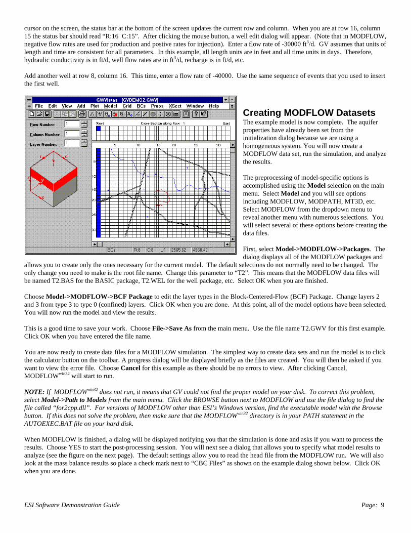
Now, let’s change the font size used for the rowand column labels. All text used to annotate theGV model may be modified in terms of fontstyle and size. To change the font for the rowand column labels, select Grid->Options andclick the font button. Change the font size to 8points and click OK to return to the GridOptions dialog. Click OK again to return to theGV menu.
You will now import a base map to display withthe model. Select File->Map->GW Vistas. Afile open dialog will be displayed. Choose themap called “t2.map”, which can be found in thedemo directory (the default location isc:\esidemo). After importing the map, selectView->Full->Screen to fit everything back inthe GV window. Your screen should now looksimilar to the one shown below.
Adding Rows & Columns
GV has four different modes when designing themodel. These include Analytic Elements, Grid,Boundary condition, and Property zones. Thedesign operation that you may perform isdetermined on the Edit menu. Select Edit fromthe main menu. At the bottom of the pulldownmenu you will see selections entitled Grid,Aquifer Properties, Boundary Conditions, andAnalytic Elements. A check mark appears nextto the option that is the current selection and theappropriate button is pushed down on the
toolbar. The button represents Analytic
Elements, represents Boundary Conditions,
stands for Property Zones, and represents Grid operations. The Grid optionallows you to add, delete, and move rows,
columns, and layers. Aquifer Properties refers to assigning physical properties (e.g., hydraulic conductivity) to each cell in the model.Analytic Elements refers to the grid-independent boundary conditions in GV. You will see the buttons on the right side of the toolbarchange depending upon which button is pressed down. This customization provides you with the most commonly used commands foreach mode.
GV gives you the ability to insert, move, and delete rows, columns, and layers. In order to perform these operations, you must be in
“grid” mode. This is accomplished by selecting Edit->Grid from the main menu or by pressing the button on the toolbar. Theword grid will appear in one of the panes of the status bar at the bottom of the GV window.
Once in grid mode, the cursor behaves differently than in other modes. When you are close to a row or column grid line, the cursorchanges shape to either a left-right or up-down arrow. Pressing the left mouse button when this cursor appears allows you to slide therow or column line to a new position. You may not slide it beyond the adjacent row or column, however.You may insert or delete rows, columns, and layers using the menu commands. These are fairly straight forward. Select the command(Grid->Insert->Row for example), move the cursor on the screen, and click the left mouse button. When deleting a row or column,

ESI Software Demonstration Guide Page: 8
the row or column closest to the cursor is deleted. Layers may be added above or below the current layer (the current layer isdisplayed as L:1,2,3,... on the status bar).
The right mouse button has a special use in GV. When you are in Grid mode, the right mouse button inserts a row or column into themodel or deletes the nearst row or column. The current grid operation (shown at the bottom of the Grid menu) determines what isadded or deleted. To add rows or columns to the model, select Grid->Insert Row or Grid->Insert Column from the menu. To deleterows or columns from the model, select Grid->Delete Row or Grid->Delete Column from the menu. A check mark appears next tothe type of action that GV will take when the right mouse button is clicked in Grid mode. The appropriate button is also pushed down
on the toolbar ( to delete a row, to insert a row, to delete a column, and to insert a column).
In this example, you will add two rows and two columns to the model. First, click the button on the toolbar to enter Grid mode.Next, split row 15 into two new rows by placing the cursor anywhere within row 15 and click the right mouse button. Repeat thisprocedure for the next row to the south (Row 16 of the original model). When you insert a row or column, the default behavior is tosplit the current cell in half. You may change the way rows/columns are inserted by selecting Grid->Options.
Adding columns works the same way. Start by selecting Grid->Insert Column to place a check mark next to “Insert Column” on theGrid menu. Now split columns 14 and 15 just like you did for rows 15 and 16 above. Position the cursor within Column 15 and clickthe right mouse button. Repeat for the original column 16. Your screen should look like the one shown below:
Adding Boundary Conditions
You will now select Boundary Conditions as thecurrent design mode so that you can addboundary condition cells to the model design.Select Boundary Conditions on the Editpulldown menu. You may also click the toobar
icon .
In this example, you will add a column ofconstant heads along the left edge of the modelin layer 1. You will then add two wells in thebottom layer (layer 3) of the model.
The easiest way to set a large number ofboundary conditions is to use the Windowcommand. Select BCs->Insert->Window from
the main menu (or from the toolbar). Thecursor will change shape and appear like a mini-
finite-difference grid. Move the cursor to the upper left corner of the model (row 1, column 1) and press the left mouse button. Holdthe mouse button down and move the cursor to the lower left corner (row 30, column 1). Release the mouse button and a dialogappears to confirm the coordinates of the window that you just created. Simply press the OK button to accept these coordinates. Next,a constant head dialog appears. The only item that must be changed is the value of constant head. Change this value to 150 ft. Noticethat by default the boundary condition is “steady-state”. This means that the boundary cells will be active during the entire simulation.In MODFLOW, constant heads are active for the entire simulation and cannot be changed. Your screen should now look like the oneshown on the next page.
Now, move to layer 3 of the model. The easiest way to change layers is by clicking the “+” button next to “Layer” on the 3D cube(called the Reference Cube) that is on the left side of the screen. Click the “+” button twice to get to Layer 3. The model will beredrawn and the constant head cells will disappear. This happens because these constant head cells were defined in layer 1 (the toplayer) and we are now viewing the bottom layer of the model. You should still see one constant head in the upper left corner of thecross-section view however.Select BCs->Well from the main menu. This places a check mark next to the word “Well” indicating that we are now editing wells.Next, select BCs->Insert->Single Cell. Move the cursor to row 16, column 15 and click the left mouse button. (You could also add awell by simply moving the cursor to row 16, column 15 and clicking the right mouse button.) You will notice that as you move the
ESI Software Demonstration Guide Page: 9
cursor on the screen, the status bar at the bottom of the screen updates the current row and column. When you are at row 16, column15 the status bar should read “R:16 C:15”. After clicking the mouse button, a well edit dialog will appear. (Note that in MODFLOW,negative flow rates are used for production and postive rates for injection). Enter a flow rate of -30000 ft3/d. GV assumes that units oflength and time are consistent for all parameters. In this example, all length units are in feet and all time units in days. Therefore,hydraulic conductivity is in ft/d, well flow rates are in ft3/d, recharge is in ft/d, etc.
Add another well at row 8, column 16. This time, enter a flow rate of -40000. Use the same sequence of events that you used to insertthe first well.
Creating MODFLOW DatasetsThe example model is now complete. The aquiferproperties have already been set from theinitialization dialog because we are using ahomogeneous system. You will now create aMODFLOW data set, run the simulation, and analyzethe results.
The preprocessing of model-specific options isaccomplished using the Model selection on the mainmenu. Select Model and you will see optionsincluding MODFLOW, MODPATH, MT3D, etc.Select MODFLOW from the dropdown menu toreveal another menu with numerous selections. Youwill select several of these options before creating thedata files.
First, select Model->MODFLOW->Packages. Thedialog displays all of the MODFLOW packages and
allows you to create only the ones necessary for the current model. The default selections do not normally need to be changed. Theonly change you need to make is the root file name. Change this parameter to “T2”. This means that the MODFLOW data files willbe named T2.BAS for the BASIC package, T2.WEL for the well package, etc. Select OK when you are finished.
Choose Model->MODFLOW->BCF Package to edit the layer types in the Block-Centered-Flow (BCF) Package. Change layers 2and 3 from type 3 to type 0 (confined) layers. Click OK when you are done. At this point, all of the model options have been selected.You will now run the model and view the results.
This is a good time to save your work. Choose File->Save As from the main menu. Use the file name T2.GWV for this first example.Click OK when you have entered the file name.
You are now ready to create data files for a MODFLOW simulation. The simplest way to create data sets and run the model is to clickthe calculator button on the toolbar. A progress dialog will be displayed briefly as the files are created. You will then be asked if youwant to view the error file. Choose Cancel for this example as there should be no errors to view. After clicking Cancel,MODFLOWwin32 will start to run.
NOTE: If MODFLOWwin32 does not run, it means that GV could not find the proper model on your disk. To correct this problem,select Model->Path to Models from the main menu. Click the BROWSE button next to MODFLOW and use the file dialog to find thefile called “for2cpp.dll”. For versions of MODFLOW other than ESI’s Windows version, find the executable model with the Browsebutton. If this does not solve the problem, then make sure that the MODFLOWwin32 directory is in your PATH statement in theAUTOEXEC.BAT file on your hard disk.
When MODFLOW is finished, a dialog will be displayed notifying you that the simulation is done and asks if you want to process theresults. Choose YES to start the post-processing session. You will next see a dialog that allows you to specify what model results toanalyze (see the figure on the next page). The default settings allow you to read the head file from the MODFLOW run. We will alsolook at the mass balance results so place a check mark next to “CBC Files” as shown on the example dialog shown below. Click OKwhen you are done.

ESI Software Demonstration Guide Page: 10
GV automatically contours the head results for thecurrent layer and cross-section views. The resultingcontours for layer 3 and for the cross-section along row1 are shown below. Your screen should look similar,unless you have changed to another layer. You maycontour any layer or cross-section by simply changingthe settings on the reference cube. For example, if youclick the “-“ button next to Layer on the cube, the layerabove the current layer will be contoured and displayed.Similarly, if you select a new cross-section, it will alsobe recontoured. You may plot velocity vectors on themap and cross-section by selecting Plot->What toDisplay… from the main menu and placing a checkmark next to Vectors on the dialog. You may alsoproduce a color flood map by placing a check next to
“Color Flood”. You display all or none of thesegraphics using this dialog.
GV gives you full control over the contouring ofMODFLOW results. You may change thecontour interval, the font used to draw contours,the distance between contour labels, etc. Thesechanges are made by selecting Plot->Contour->Parameters (Plan). Change the startingcontour level to 149.0 and the contour intervalto 0.2 ft. Also, change the font size to 10 points.This is done by clicking the font button on thedialog. Click OK when you are done. A dialogwill then tell you that the view should berecontoured. Click OK to proceed.
Other Types of Plots
GV provides you with the tools to create manytypes of maps and graphs that are useful inanalyzing model results. These are accessed
from the Plot menu. We will explore a few of these plots now.
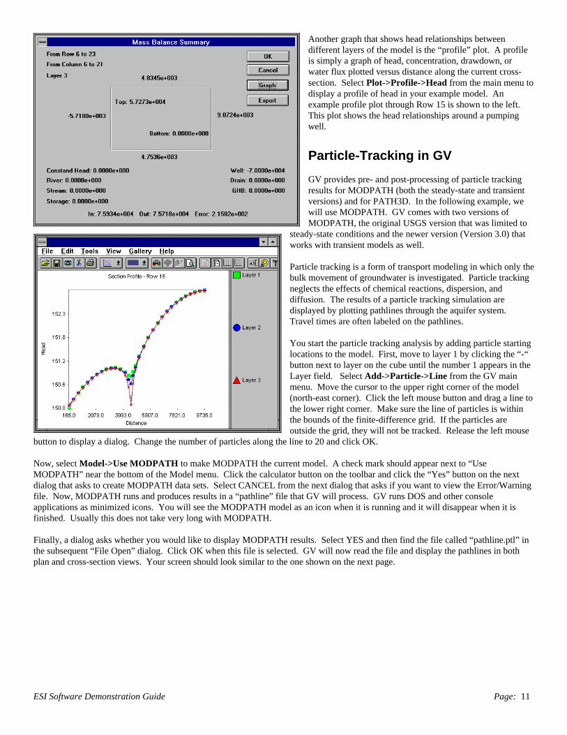
Select Plot->Mass Balance->Window from the main menu.Next drag a rectangular region on the screen. After you releasethe left mouse button, a dialog appears summarizing the flow ofwater into and out of the rectangular region you defined. Thesummary includes any boundary conditions that are within thatrectangle in the current layer. An example is shown on the nextpage.
You may produce a bar chart of the mass balance results bysimply clicking on the “Graph” button on the dialog. An exampleis shown to the left. Another useful mass balance feature of GVis that the flux rate of water into or out of a boundary cell isdisplayed on the status bar when the cursor moves over aboundary cell. Try this feature by moving the cursor over aconstant in layer 1. The flow rate into the constant head for Row1, Column 1 should be about -1561 ft3/d (NOTE: You must be inBoundary Condition mode to view fluxes; press the “B” button on
the tool bar to enter BC mode). The negative sign is the MODFLOW convention for water being removed from the aquifer.
ESI Software Demonstration Guide Page: 11
Another graph that shows head relationships betweendifferent layers of the model is the “profile” plot. A profileis simply a graph of head, concentration, drawdown, orwater flux plotted versus distance along the current cross-section. Select Plot->Profile->Head from the main menu todisplay a profile of head in your example model. Anexample profile plot through Row 15 is shown to the left.This plot shows the head relationships around a pumpingwell.
Particle-Tracking in GV
GV provides pre- and post-processing of particle trackingresults for MODPATH (both the steady-state and transientversions) and for PATH3D. In the following example, wewill use MODPATH. GV comes with two versions ofMODPATH, the original USGS version that was limited to
steady-state conditions and the newer version (Version 3.0) thatworks with transient models as well.
Particle tracking is a form of transport modeling in which only thebulk movement of groundwater is investigated. Particle trackingneglects the effects of chemical reactions, dispersion, anddiffusion. The results of a particle tracking simulation aredisplayed by plotting pathlines through the aquifer system.Travel times are often labeled on the pathlines.
You start the particle tracking analysis by adding particle startinglocations to the model. First, move to layer 1 by clicking the “-“button next to layer on the cube until the number 1 appears in theLayer field. Select Add->Particle->Line from the GV mainmenu. Move the cursor to the upper right corner of the model(north-east corner). Click the left mouse button and drag a line tothe lower right corner. Make sure the line of particles is withinthe bounds of the finite-difference grid. If the particles areoutside the grid, they will not be tracked. Release the left mouse
button to display a dialog. Change the number of particles along the line to 20 and click OK.
Now, select Model->Use MODPATH to make MODPATH the current model. A check mark should appear next to “UseMODPATH” near the bottom of the Model menu. Click the calculator button on the toolbar and click the “Yes” button on the nextdialog that asks to create MODPATH data sets. Select CANCEL from the next dialog that asks if you want to view the Error/Warningfile. Now, MODPATH runs and produces results in a “pathline” file that GV will process. GV runs DOS and other consoleapplications as minimized icons. You will see the MODPATH model as an icon when it is running and it will disappear when it isfinished. Usually this does not take very long with MODPATH.
Finally, a dialog asks whether you would like to display MODPATH results. Select YES and then find the file called “pathline.ptl” inthe subsequent “File Open” dialog. Click OK when this file is selected. GV will now read the file and display the pathlines in bothplan and cross-section views. Your screen should look similar to the one shown on the next page.

ESI Software Demonstration Guide Page: 12
Model Calibration with GVCalibration is one of the most complex parts ofapplying groundwater models. GV assistsmodel calibration in three ways: (1) calculationof calibration statistics for head, drawdown,concentration, or flux, (2) automated parametersensitivity analysis, and (3) support for thePEST model-independent calibration software.You start by adding calibration targets to themodel. A calibration target is a point in theaquifer where a measurement of head,drawdown, concentration, or flux has beenmade. Calibration targets may be either steady-state or transient. When you run the model tocompare against the target values, GV reads themodel results and interpolates the model resultin both space and time to compute an error orresidual. Analysis of residual statistics is apowerful way of determining calibration qualityand guiding further refinements to the model.The following exercise will illustrate the
calculation of calibration statistics and automatic sensitivity analysis. PEST support is not covered in this demo.
We will start by defining 16 head target locations in our example model. Rather than type in the data manually, you will import a textfile containing the target data. GV provides many data import features for calibration targets, boundary conditions, aquifer properties,and base maps. Select Plot->Calibration->Import Targets from the main menu. Find the file called “targets.dat”, which should bein the demo directory (default is c:\esidemos). Click OK when you have found it. GV will report the number of targets successfullyimported. In this example, there should be 16. The targets will appear on the plan view as small blue dots. Targets are only displayedfor the layer in which they are defined. You should see 6 in layer 1, 5 in layer 2, and 5 in layer 3. You may edit target information by
double-clicking on a target symbol (You must be in Analytic Element mode, however; click the button on the tool bar to edittargets in this manner).
You will need to import model results again in order to computethe calibration statistics. Select Plot->Import Results and clickOK on the dialog. All of the options should be set properly fromthe last run you made. You may view the calibration statistics byselecting Plot->Calibration->Statistics/Plots… A dialog isdisplayed that allows you to select the type of targets to use in thecalculation (head, concentration, drawdown, or flux). You mayalso plot only selected ranges of layers. To view the statistics forthis model, click the Statistics button. The residual sum ofsquares should be about 7.06E-03 ft2. Click OK to leave thisdialog. Now click the Plot button. A graph of observed vs.computed heads is displayed. Targets are color coded by layer.Your plot should be similar to the one shown to the left.
Another way to view the target residuals (errors) is to post themon the contour map. You do this by selecting Plot->Calibration->Post Residuals. Target residuals are posted when a check markis displayed next to “Post Residuals” on this menu. In thisexample, the residuals are too small to read. You may change the
font size by selecting Plot->Calibration->Target Options. Click the font button to change the size or font. Select View->Refresh toredraw the window with the new font.
Sensitivity analysis is an integral part of model calibration. Sensitivity analysis is the process whereby model parameters or boundaryconditions are altered slightly and the effect on model calibration statistics is observed. By producing a series of simulations withdifferent values for a single model parameter, you get a feel for how a parameter may be modified in order to achieve a bettercalibration. This is a tedious process because many simulations are required for each parameter and there are often many parameters

ESI Software Demonstration Guide Page: 13
to analyze. GV provides you with an automated way of performing a sensitivity analysis that greatly improves the process. Yousimply choose a parameter type, the number of simulations, and a parameter multiplier for each simulation. GV then runs MODFLOWthe desired number of times and produces a sensitivity plot. For each simulation, GV multiplies your initial parameter value by themultiplier you specify. After all of the simulations are finished, GV plots calibration statistics versus parameter multiplier to visuallyshow the results of the analysis.
You start a sensitivity analysis by selecting Model->SensitivitySetup. Select Kz as the parameter to vary. Keep the default ofZone number 1 and 5 simulations. Click on the “Multipliers”button. Enter the values 0.2, 0.5, 1.0, 1.5, and 2.0 for simulations1 through 5, respectively. Click OK when you are done and clickOK on the main dialog. Running the analysis is as simple asselecting Models->Run Sensitivity from the main menu. Youwill see MODFLOW flash on your screen five times and after thelast simulation a dialog will ask whether you would like to see theresults. Select “Yes” and you are asked to choose a variable toplot for each run. The choices include sum of squared residuals,residual mean, residual standard deviation, average drawdown,and total flux to a designated boundary condition reach. A plot ofresidual sum of squares vs. multiplier is displayed at the left forthis example.
By producing a series of sensitivity plots, you can quicklydetermine the optimum parameter values to assign in yourcalibrated model. Of course, these parameters should be
reasonable values given your knowledge of the aquifer system.
Editing Aquifer PropertiesAquifer properties, such as hydraulic conductivity, are defined in GV using the “zone” concept (See the Help File topic entitledConcepts for a more elaborate discussion on zones). This means that you define a finite number of zones for each parameter andassign a zone number to each cell in the model. A zone number represents a fixed value for the parameter. When you first set up amodel, every parameter is assumed to be homogeneous and every cell in the model is assigned a zone number of 1. For example, youentered an initial hydraulic conductivity value of 100 ft/d in the first GV dialog. GV assigns this value to zone 1 and then assigns zone1 to each cell in the model.
GV displays zones using colors and fill patterns. To view and edit parameter zone values, select Edit->Aquifer Properties or click on
the button on the toolbar. Pull down the Props menu and you will see all of the available properties listed at the bottom of themenu. The property type with the check mark next to it is the one you are currently viewing and editing. Simply click on anotherproperty type to change the current property.
If the parameter zone is homogeneous, GV does not fill in the cells in your model. However, you may see the zone and property valueassigned to cells by simply moving the cursor around the grid. The zone number and property value assigned to that number aredisplayed on the left side of the status bar at the bottom of the GV window. Do this now and you should see Zone:1 Kx=100.0. Thismeans that the cells in you model are assigned a hydraulic conductivity (K) zone number of 1 and that zone 1 represents a K value of100.0 ft/d.
We will now change the distribution of hydraulic conductivity in your model by first defining another zone value and then assigningthis new zone to some cells in your model. The first step is to modify the database of zone numbers for hydraulic conductivity. Select
Props->Property Values->Database or press on the toolbar. You will see a dialog that lists zone numbers on the left (NOTE:these are NOT layer numbers). There are three columns labeled Kx, Ky, and Kz. These are the three directional values of hydraulicconductivity. You should also see that zone 1 has been assigned values of 100.0, 100.0, and 10.0 for these three parameters,respectively. All other zone numbers in the database have values of zero. Now, change the Kx, Ky, and Kz values for zone 2 to 25.0,25.0, and 2.5. Click OK to save these values.
By changing the value of the property assigned to zone 2, you have not changed the model at all because no cells are currently assignedzone 2! You have simply allowed for the possibility that a value of 25.0 ft/d may be assigned for hydraulic conductivity. To actuallychange certain cells to this new property value, select Props->Set Zone Numbers->Window. Now move the cursor to a location

ESI Software Demonstration Guide Page: 14
within the model and drag a rectangle on the screen. Release the left mouse button and you will see a dialog asking for the zonenumber to assign to this region. Enter a value of 2 and click the OK button (or simply hit the Enter key). The screen will now beredrawn and you should see blue cells for the region covered by zone 1 and red for the region covered by zone 2. As you add morezone numbers, the colors change so that blue is assigned to zone 1 and red to the highest zone. A spectrum of colors is assignedbetween the two extremes. You may change the color and pattern assigned to each zone by selecting Props->Property Values->EditZone Colors and Props->Property Values->Edit Zone Patterns.
The Future of GV…
ESI is committed to making GV the most comprehensive and least expensive modeling platform in the industry. We have manyenhancements planned for the near future. Many of these enhancements will be sent to GV users free of charge or distributed overInternet. The following are some of the new features that will be added over the coming months:
Telescopic Mesh Refinement (TMR)TMR is the ability to create a new refined model covering a subregion of a larger model. The new model has smaller grid spacings andusually more nodes than the large-scale model. This technique is useful for performing transport modeling over a portion of theoriginal model. The TMR technique applies boundary conditions from the regional model to the subregional model based upon theuser’s choice of constant head, constant flux, or head-dependent flux boundary conditions. These boundaries are interpolated from thelarger-scale model automatically by GV. The small-scale model captures all of the complexity of the regional model and preserves theregional flow effects at the local scale. TMR is planned for release in GV by the end of September 1996.
3D Graphical DisplaysIn order to keep the price of GV as low as possible, ESI will not build three-dimensional visualization directly into GV. Rather, weintend to offer file export features in GV that will allow you to use whatever graphics program you wish. The supported visualizationpackages will include (from least to most expensive): Slicer by Fortner Research (formerly SpyGlass), Environmental Workbench bySSESCO, and EVS. Many other packages can be supported using GV’s generic 3D data export feature. These file export options areexpected to be complete by the end of October 1996.
Stochastic SimulationGV will be enhanced this fall to include pre- and post-processing capabilities for stochastic simulation using Stochastic MODFLOW.ESI, in cooperation with the author of Stochastic MODFLOW, will offer a free upgrade to GV for these stochastic enhancements and afee for the purchase of Stochastic MODFLOW for Windows. You will be able to perform Monte Carlo simulations using bothMODFLOW and MODPATH. These enhancements are planned for January 1997.
Automated Calibration TechniquesGroundwater Vistas already offers the most powerful set of calibration features of any modeling system. The most significant toapplied modelers is the automatic sensitivity analysis as demonstrated above. The automatic sensitivity analysis will be taken one stepfurther to include a nonlinear least-squares approach to model calibration. You will simply choose which parameters to estimate, setbounds for the estimated parameters, and GV will run MODFLOW, MODFLOWT, MODFLOW-SURFACT, or MT3D many times toperform the least squares analysis. While there are several such inverse models on the market (including PEST which comes with GVin a trial version), GV will be unique in providing you the ability to monitor the progress of the calibration and intervene during theprocess. Automated Calibration is planned for late 1996.

ESI Software Demonstration Guide Page: 15
MODFLOWwin32 Demo!
MODFLOWwin32 is Environmental Simulation’s version of the popular USGS groundwater flow model. It has all of the features of otherMODFLOW versions, including the newest packages added over the years since MODFLOW’s original release by the USGS. These newpackages include the Stream Routing Package, Aquifer Compaction Package, Horizontal Flow Barrier Package, BCF2 and BCF3Packages, and the new PCG2 solver. In addition, MODFLOWwin32 will create files for use with MODPATH (a particle-tracking model)and MT3D (a solute transport model). MODFLOWwin32, as its name implies, is a 32-bit program designed to address all of the memoryavailable to Windows. The software will run in all versions of Windows including Version 3.1, 3.11, Windows 95, and Windows NT.
MODFLOWwin32 is a true Windows program; not just a DOS program that will run in Windows’ DOS box. A comprehensive contouringprogram, called Contourwin32, is included with MODFLOWwin32 to provide for post-processing of MODFLOW simulation results. Bothhead and drawdown may be contoured from any time-step, stress period, or layer. You may also overlay a base map in WinFlow,QuickFlow, ModelCad, and DXF formats. Particle-tracking results from MODPATH (not included with this MODFLOWwin32) may alsobe displayed on the contour maps. In addition, the finite-difference grid may be plotted over the contours.
MODFLOWwin32 does not include any preprocessing software; however, you may purchase ESI’s Groundwater Vistas preprocessingsoftware at a special price when you also buy MODFLOWwin32. The cost of MODFLOWwin32 bundled with Groundwater Vistas is half thecost of Visual MODFLOW and also much less expensive than PMWIN or ModelCad.
This demonstration version of MODFLOWwin32 is fully functional with the following limitations: (1) MODFLOW has been limited to thesize of the demo problem (about 2,700 nodes), and (2) Contourwin32 will not print or save files. (Please note that you must be runningWindows Version 3.1 or higher with at least 4 megabytes of RAM and 4 megabytes of disk space available.) We hope that this demoversion will assist you in your decision to purchase MODFLOWwin32. If you have any questions, please feel free to give us a call.

ESI Software Demonstration Guide Page: 16
MODFLOW Features
MODFLOWwin32 is ESI’s version of this popular groundwater flow model, originally developed by the USGS. MODFLOW is a 3Dfinite-difference groundwater flow model and there are many versions available. Unlike MODFLOW versions from other vendors,however, ESI’s MODFLOWwin32 was developed specifically for Microsoft Windows (Win32s) and Windows NT. Using a uniquetechnology, MODFLOWwin32 runs as a DLL which is controlled by a shell program or by ESI’s Contourwin32 which is provided withMODFLOWwin32.
MODFLOWwin32 contains all of the popular add-on packages (BCF2, BCF3, PCG2, HFB, Compaction, Stream Routing) and is a 32-bit program utilizing all available memory. Contourwin32 is a postprocessor for contouring MODFLOW results and displaying particletrace pathlines computed by MODPATH. The following are a list of capabilities for this unique software combination:
MODFLOWwin32:
ÿ Runs 10 to 20 percent faster than other versions of MODFLOW for DOS!ÿ Contains the BCF2, BCF3, PCG2, STREAM Routing, and Aquifer Compaction Packages;ÿ User interface organizes file names and allows user to “abort” the simulation or force convergence when the solution oscillates;ÿ Uses all memory available to Windows, including virtual memory;ÿ Runs as a 32-bit DLL in Windows V3.1+, Windows NT, and Windows 95;ÿ Reads files created by all popular MODFLOW preprocessors;ÿ All MODFLOW manuals have been reformatted as Windows Help files;ÿ Provides several user-selectable levels of multi-tasking, even under Windows V3.1;ÿ Iteration data displayed as MODFLOW runs.
Contourwin32:
ÿ Included with MODFLOWwin32!ÿ Displays contours of head and drawdown for any layer and for subregions within the model;ÿ Overlay base maps in DXF, ModelCad, or WinFlow format;ÿ Contour head and drawdown while MODFLOWwin32 is running;ÿ WYSIWYG printing with print preview and user-defined margins to any Windows device;ÿ Export contour maps in Spyglass, Geosoft, SURFER, DXF, and Windows Metafile formats;ÿ Displays particle traces from MODPATH;ÿ Displays finite-difference grid;ÿ Annotate maps with scale bar, titles, arrows & travel times on particle traces;ÿ Computes calibration target statistics and post residuals (errors) on map.

ESI Software Demonstration Guide Page: 17
Exploring MODFLOWwin32
The MODFLOWwin32 demonstration, described below, introduces you to most of the important features of this software in a step-by-step example. You will be given very specific instructions to show how to use MODFLOW to solve real-world problems. In agraphical user environment such as Windows, it is difficult to tell you exactly what to do during each step, however, because many ofthe steps involve using the mouse. This demonstration provides several snap-shots of the MODFLOWwin32 and Contourwin32 screensto show you what your screen should look like.
The exercise below tells you to select menu items and a short-hand method is used to indicate what menu items are to be selected. Themenu items are listed in order of selection and are separated by a “->“ symbol. For example, instead of writing the following text:
Select File from the main menu and then select Open from the pulldown menu
the following shortened version is adopted in this manual:
Select File->Open
Some instructions for using the mouse should also be explained here, although most Windows users understand these concepts. Theword “click” refers to pressing the left mouse button once and “double-click” means to press the mouse button twice in rapidsuccesion. The word “drag” means to press the left mouse button and move the mouse to another location on the screen while keepingthe button pressed down. Release the mouse button when the cursor is on the desired location.
Running a MODFLOW Model
We will start this demonstration by showing you MODFLOWwin32 and Contourwine32 separately. The final section will illustrate howthe two programs work together. To start, double-click on the MODFLOWwin32 icon now. You will see a tab dialog interface with thefollowing sections or tabs:
l Simulation - reads in a MODFLOWwin32 simulation input file (containing all data set names),l Input - allows you to specify the names of MODFLOW input files (Basic Package etc.),l Output - specify output file names (Head-save, cell-by-cell, etc.),l Progress - displays iteration and error summaries as the model runs, andl Head/Drawdown - communication with Contourwin32
You will select “Input” by clicking the mouse on the Input tab. Click the Input File button to start entering file names for aMODFLOW simulation. Select T1.BAS from the file list and click OK. This is the way you will start MODFLOWwin32 using existingMODFLOW data sets. Now, click the Run button at the bottom of the MODFLOWwin32 dialog. You will be asked to provide filenames for packages and output files needed for the simulation. Simply select the only file name given (T1.*), in the order below:
T1.BCF - Block-Centered Flow PackageT1.WEL - Well PackageT1.RIV - River PackageT1.RCH - Recharge PackageT1.SIP - SIP SolverT1.OC - Output Control
After the output control file, you must enter two additional files for computed head and drawdown. These files do not exist, so no filenames appear in the dialog. Simply type the following names in the order shown below:
T1.HDS You will type in this name for head output for contouringT1.DDN You will type in this name for drawdown output for contouring
After entering the drawdown file name (T1.DDN), click the Progress tab to see how the simulation progresses. This particular runconsists of 2 stress periods with 20 time steps each. The model is relatively small so the simulation should not take long. Whenfinished, your screen should look like the screen shown below:

ESI Software Demonstration Guide Page: 18
Now, you will save this simulation in aMODFLOWwin32 file for processing bythe contouring program. Click theSimulation tab and then click the SaveAs button. Enter a file name ofT1.MFW. Click the OK button whenfinished. Finally, click the Close buttonat the bottom of the dialog to end theMODFLOW session.
Contouring the Results
We will now show you the procedure forcontouring MODFLOWwin32 output.Double-click the Contourwin32 icon.Start a new map by selecting File->Newfrom the menu. You may also press the
button on the toolbar below themenu. To load a set of heads ordrawdowns from the MODFLOWsimulation, select File->Model andchoose the T1.MFW file. Click OK when you are finished selecting the MODFLOWwin32 file. After a few seconds, a list of heads anddrawdowns are presented showing the variable type (Head or Drawdown), Stress Period number, Time Step number, and Layernumber. Choose Heads in Stress Period 2, Time Step 20, Layer 3 and click the OK button. Head contours will be displayed on yourscreen for the selected time and layer.
Overlay a digitized base map by selectingFile->Map->WinFlow from the menu.Select T2.MAP and click OK. A furtherdialog is displayed asking for coordinatetransformation details. Simply click OKto accept the defaults (If you are usingModelCad, you can enter the offsets androtation to adjust the map to the modelgrid using this dialog). Your screenshould look like the one shown at the left.
Contourwin32 can plot the finite-differencegrid on the contour map. Select Options->Grid from the menu. Click “DisplayNumbers” for both rows and columns.Click “Display Grid” to plot the grid onthe screen. Finally, change the Interval to5 so that row and column numbers arelabelled every 5 cells. Click OK whenyou are done and your screen should looklike the one at the top of the next page:
By default, Contourwin32 selects a contourinterval to show 10 contour levels. You
may change the contouring parameters by selecting Options->Contour->Parameters from the menu. Change the minimum contourlevel to 150.0 ft and the contour interval to 0.2 ft. Click OK when you are finished. A message will then appear asking you if youwant to recontour using these parameters. Select Yes to do this.

ESI Software Demonstration Guide Page: 19
Although MODPATH is not part of the MODFLOWwin32 package (a version is included with Groundwater Vistas, however),Contourwin32 will display MODPATH results and MODFLOWwin32 output files are compatible with most MODPATH versions fromother vendors. We have provided a MODPATH output file with this demo to show you how to process particle-traces.
Select Options->Particle from the menu.Click the Browse button to show a list offiles and select the file calledPATHLINE.PTL. Also, click the“Display traces” button on the dialogafter selecting the file. Click OK whenyou are finished. Your screen shouldlook like the one shown below:
Particle traces may be annotated withtravel time and arrows. Select Options->Arrow from the menu and click“Display Arrows” on the dialog. ClickOK when you are done. This causesarrow-heads to be displayed on thetraces. You can add time postings usingOptions->Time.
Contouring WhileMODFLOW is Running
We will now show you howMODFLOWwin32 and Contourwin32 canwork together. Under all versions ofWindows, the two programs(MODFLOW and Contour) are totallylinked. MODFLOWwin32 can start theContourwin32 program and vice versa.
Double-click the MODFLOWwin32 iconto run the model again and click theOpen button in the MODFLOW dialog.Select the T1.MFW file and click OK.Start the model simulation by clickingthe Run button. Now click theHead/Drawdown tab to see heads anddrawdown data written to the outputfiles. When some appear on the screen,select one by clicking on the linecontaining the desired variable, stressperiod, time step, and layer number.Choose any one and click the Contourbutton. This causes MODFLOWwin32 torun Contourwin32 and pass the data toContourwin32, which will open a newdocument and contour the data. Youshould see contours being displayedbehind the MODFLOWwin32 dialog.Press ALT-TAB to see the entire map and ALT-TAB again to get back to MODFLOWwin23.

ESI Software Demonstration Guide Page: 20
WinFlow Demo!
WinFlow is a powerful yet easy-to-use groundwater flow model. The model is similar to Geraghty & Miller's popular QuickFlowmodel, which was developed by Jim Rumbaugh, one of the authors of WinFlow. The most notable improvement over QuickFlow iscompatibility with Microsoft WindowsTM V3.1. It is not just a DOS program that happens to run under Windows in a DOS shell.WinFlow is a true Windows program incorporating a multiple document interface (MDI). The following discussion explains the basicfeatures of WinFlow, how to install the demonstration version of the software, and the many differences between WinFlow andQuickFlow.
WinFlow is an interactive, analytical model that simulates two-dimensional steady-state and transient ground-water flow. The steady-state module simulates ground-water flow in a horizontal plane using analytical functions developed by Strack (1989). The transientmodule uses equations developed by Theis (1935) and by Hantush and Jacob (1955) for confined and leaky aquifers, respectively.Each module uses the principle of superposition to evaluate the effects from multiple analytical functions (wells, etc.) in a uniformregional flow field.
The steady-state module simulates the effects of the following analytic elements in two-dimensional flow: wells, uniform recharge,circular recharge/discharge areas, and line sources or sinks. Any number of these elements may be added to the model, including auniform regional hydraulic gradient. The model depicts the flow field using streamlines, particle traces, and contours of hydraulichead. The streamlines are computed semi-analytically to illustrate ground-water flow directions. Particle-tracking techniques areimplemented numerically to compute travel times and flow directions. Both confined and unconfined aquifers are simulated withthe steady-state module.
The transient module simulates the effects of wells, circular ponds, linesinks, and a uniform regional gradient for confined and leakyaquifers. Numerical particle-tracking is also available in the transient module. The transient module computes hydraulic heads usingthe Theis (1935) equation for confined aquifers and the Hantush and Jacob (1955) equation for leaky aquifers.
WinFlow is simple to use and highly interactive, allowing you to create an analytical model in minutes. The software features standardWindows pulldown menus and dialogs to facilitate the model design. The model is recomputed and recontoured either by selecting amenu item or by pressing a toolbar button. Streamlines and particle-traces are added interactively and recomputed each time new wellsor other elements are added.
WinFlow can import a Drawing Interchange Format (DXF) file (from AutoCAD for example) to use as a digitized base map.QuickFlow and ModelCad-format map files may also be imported into WinFlow. The digitized map gives the modeler a frame ofreference for designing the analytical model.
WinFlow produces report-quality graphics using any Windows device driver. Output may also be exported to a wide variety of filetypes, including SURFER, Geosoft, Spyglass, Windows Metafiles, and AutoCAD-compatible DXF files.
WinFlow Features
The WinFlow demonstration version is fully functional, with the exception that models cannot be saved or printed. All other featuresare functional, including the on-line help system which contains the entire WinFlow manual. Press F1 at any time to view the Helpfile. WinFlow has the same basic capabilities as Geraghty & Miller’s QuickFlow software, although many features are different orenhanced. The features that WinFlow has in common with QuickFlow include the following:
ÿ Simulates both steady-state and transient flow;ÿ Simulates both unconfined and confined aquifers;ÿ Simulates effects of wells, linesinks, ponds, and recharge;ÿ Imports map files in DXF format, QuickFlow format, or ModelCad format;ÿ Visualizes model results with water-level contour maps;

ESI Software Demonstration Guide Page: 21
ÿ Illustrates groundwater flowpaths using streamlines and particle traces;
The most notable enhancement is that WinFlow is a standard Windows MDI (Multiple Document Interface) application. ExperiencedQuickFlow users should scan the following list to get a feel for these enhanced features:
ÿ Linesinks and ponds included in the Transient model;ÿ Calibration targets and calculation of calibration statistics;ÿ Each analytic element may have a title with full font selection;ÿ Double-click an element to edit;ÿ Click and drag to reposition elements, streamlines, or particles;ÿ Click and drag to resize linesinks and ponds;ÿ Multiple document interface (MDI) allows multiple models to be open at the same time;ÿ Cut, copy, and paste elements to/from the clipboard;ÿ Maps may be printed using any Windows device driver;ÿ Coordinates and head are displayed as the cursor is moved;ÿ Full context-sensitive help system (the entire manual is on-line);ÿ DXF file import from within WinFlow;ÿ Common commands are available on the Toolbar; andÿ Drag-and-drop input files into the WinFlow window.
Exploring WinFlow
After installing the demo version of WinFlow, you have several alternatives for exploring its features. The first is to run through thedemonstration described below. This describes most of the basic WinFlow features. Another option is to run the example WinFlowdata sets contained on the demo disk. Select File from the main menu and Open from the dropdown menu. You should see three files(ex1.wfl, ex2.wfl, and ex3.wfl). Select any of the three examles and choose OK. Use the on-line help and your own intuition toexplore from here (Press F1 at any time for help). The final alternative is to load existing QuickFlow files. This is done by selectingFile and Open from the main menu. Next, select QuickFlow under the button labeled “List Files of Type” (NOTE: your QuickFlowfiles must end in the extention qfl).
Introduction
The WinFlow demonstration guide introduces you to most of the important features of this software in a step-by-step example. Youwill be given very specific instructions to show how to use WinFlow to solve real-world problems. In a graphical user environmentsuch as Windows, it is difficult to tell you exactly what to do during each step, however, because many of the steps involve using themouse. This demonstration guide provides several snap-shots of the WinFlow screen to show you what your screen should look like.In addition, the final data files are provided so that you may skip most of the following steps but still get a feel for how WinFlowworks.
The demonstration guide tells you to select menu items and a short-hand method is used to indicate what menu items are to be selected.Thus, the menu items are listed in order of selection and are separated by a “->“ symbol. For example, instead of writing thefollowing text:
Select File from the main menu and then select Open from the pulldown menu
the following shortened version is adopted in this manual:
Select File->Open
Some instructions for using the mouse should also be explained here, although most Windows users understand these concepts. Theword “click” refers to pressing the left mouse button once and “double-click” means to press the mouse button twice in rapidsuccesion. The word “drag” means to press the left mouse button and move the mouse to another location on the screen while keepingthe button pressed down. Release the mouse button when the cursor is on the desired location.

ESI Software Demonstration Guide Page: 22
Setting Up the Model
Start the WinFlow program by double-clicking on its icon, . You should see a simple menu displayed above a blank window. A
new model is started by selecting File->New or by pressing the button on the toolbar below the menu. Now you can start todesign the model.
The first step in most models is to import a base map that will serve as your reference point for the model. Two maps have beensupplied for use in the demonstration guide. You will import the map called PLUME1.MAP. Select File->Map->WinFlow andchoose plume1.map in the standard Windows file dialog. Your screen should now look like the screen shown below. Notice the greenarrow in the center of the screen, which denotes the location of the “reference head”. The reference head is actually located at thecenter of the base of the arrow. The reference head is a point in the aquifer where the head is fixed during the simulation and cannotchange. This is analogous to a “constant head” in a numerical model, such as MODFLOW. You must be careful to locate thereference head as far from the area of interest in your model (e.g., pumping wells) as you can.
In this example, we want to move the reference head to the upper left portion of the screen. You should now move the green arrow to
coordinates X=167600 and Y=163180. Place the cursor over the green arrow until you see the cursor. Now, hold down the leftmouse button and drag the green arrow to the desired coordinates. The coordinates are displayed in the lower right corner of the statusbar at the bottom of the screen. The coordinates do not have to be exact, since you will be able to edit them when you release themouse button.
Now, again place the cursor over the reference head(green arrow) and double-click the left mouse button.You will see a dialog that lists data corresponding to thereference head. Check the coordinates listed in thedialog and make sure the coordinates are close to theones given above. Next, change the hydraulic gradientto 1.0e-03 and the angle to 135 degrees. Click on theOK button when you are done.
The next step is to make sure that the aquifer propertiesare set correctly. Select Edit->Parameters and changethe top elevation of the aquifer to 500 ft. In the steady-state model, WinFlow automatically determines whetheran aquifer is confined or unconfined. The aquifer isunconfined when the head is below the top of the aquiferand it is confined if the head is above the top of the
aquifer. In this example, the aquifer is unconfined, so you will make the top of the aquifer very high (e.g., a large distance above thereference head value of 200 ft.). The top elevation is the only parameter to change in this example, so click the OK button.
The previous dialog contained a list of all aquifer properties in the WinFlow model. You need to maintain a consistent set of unitswhen you assign these parameters. This is done by selecting one unit of measure for length (e.g. feet) and one unit of measure for time(e.g. days). Using these examples, hydraulic conductivity has units of ft/d and pumping rates are in ft3/d.
You have now set up the most important parts of the WinFlow model! To see the results, simply select Calc->Recalculate or click the button. You should see a series of contours that are straight lines, representing the uniform regional hydraulic gradient. You will
also note that the contour interval is uneven. When a new model is started, WinFlow simply computes the maximum head differencein the model and divides this number by ten to get the starting contour interval. You should change the contouring parameters byselecting Options->Contour->Parameters. Change the minimum contour level to 198 and the contour interval to 1.0 ft. Click OKwhen you are done. WinFlow will now ask whether you would like to recontour the current model. Choose YES and your screenshould look like the one shown below.

ESI Software Demonstration Guide Page: 23
This is a good time to save your work. Select File->SaveAs and enter the name EX1 in the dialog. ClickOK when you are down. WinFlow automaticallyattaches the file extension “.wfl” to the file name.Sorry, the demonstration version does not save files, butthis is how you would do it in the full version.
Adding FeaturesMost models are more complex that the one you justcreated. Usually, you would like to analyze the effectsof pumping wells or other features. In the next section,you will add a pumping well to the model and evaluatethe capture zone of the well by adding streamlines. Youwill also learn how to change the pumping rate of thewell.
You should see a red oval shape in the center of the base map. This area is labeled “plume” and represents an area to be captured in apump-and-treat system. Add a well at the downgradient edge of the plume by selecting Add->Well or by clicking the button.Move the cursor to coordinates X=171500 and Y=160500 and click the left mouse button. The well will be added where the point ofthe arrow cursor indicates. Next, a dialog box for the well will be displayed; enter a pumping rate of 20,000 ft3/d and click the OKbutton. Note that the word “ReCalculate” appears in the status bar. This reminds you that the contours on the screen may not berepresentative of your current model. Click the calculate button to recompute the model.
The contours should show a slight cone of depression around the well you added. To see if the well captures the plume, you will needto add several streamlines. Streamlines are used to illustrate groundwater flow directions. Select Add->Streamlines->Line. You willnow drag a line along the 208 ft contour line in the lower right portion of the screen. After dragging the line, a dialog is displayed.Change the number of streamlines to 20 and click the OK button. The streamlines will then be drawn on the contour map. It is oftenuseful to add arrow-heads to the streamlines to more clearly show the direction of flow. Select Options->Arrow and change thedistance between arrows to 500 ft and the arrow size to 100. Finally, click on the “Display Arrows” field and then the OK button.
Your screen should look like the one shown below. Note that the capture zone of the pumping well does not quite cover the entire
plume area. You can increase the amount of pumping from the well by moving the cursor over the well until you see the cursor.Now, double-click on the well and the well dialog appears. Change the pumping rate to 50,000 ft3/d and recalculate the model. Thecapture zone should now cover the entire plume.
Now let’s examine other aspects of the map. The blueline on the map represents a river. Thus far, we haveignored the river in our model. WinFlow can simulatethe influence of rivers or drains using linesinks.Linesinks can be defined using either a head value or aflux value. In a head linesink, WinFlow computes theflux needed to maintain the head at the specified value atthe center of the linesink. In a flux linesink, you supplyWinFlow with the flow rate into or out of the linesinkper unit length (take the total flow and divide by thelength of the linesink). In this example, you will add 9linesinks to the model along the river to evaluate theimpact on the recovery system.
First, in order to give you a better frame of reference forthe linesinks, you will import a new map file. WinFlow
allows only one digitized map to be used at any one time. When you import a map file into a model that already has a map, WinFlowdeletes the first map and displays the second one. Select File->Map->WinFlow and choose PLUME2.MAP. This map has a series of“x”s along the river and numbers between the “x”s. You must add a head linesink between each pair of “x”s and set the head to thevalue displayed on the map.

ESI Software Demonstration Guide Page: 24
For example, you will add a head linesink in the upperleft corner at a head value of 200 ft. Select Add->HeadLinesink or click the button. Drag a line betweenthe last two “x”s on the left side of the river. A dialogwill be displayed; enter a head value of 200 ft and clickthe OK button. Now add the remaining 8 linesinks inintervals of 1 ft between the “x”s. Finally, recomputethe model and your screen should look like the one tothe left.
After adding all of the linesinks, your screen should looksimilar to the one at the left. You can see that thelinesinks have a subtle effect on the flow field. You canalso determine how much groundwater the river isgaining or losing. To find out the flow rate of a linesink,
place the cursor on a linesink (you will see the cursor) and double-click. The dialog shows the flow rate in ft3/d per ft of river. All of the linesinks are removing water from theaquifer except the one labeled 204. A linesink removes water from the aquifer if the sign on the flow rate is positive and losing waterto the aquifer if the flow rate is negative. Check thelinesink flows with your model.
You may want to compare the two models (with andwithout linesinks) more closely to determine the impactof the river on the aquifer. You could print the contourmaps using File->Print or you could have both modelsdisplayed simultaneously on your screen. You can dothis by selecting File->Open and choosing the fileEX2.WFL. By default, WinFlow overlays the twomodels so that you can only see one at a time. SelectWindow->Tile and both models will be displayed at thesame time. You can resize the windows and move themodel windows around. Try to get your screen to looklike the one at the right.

ESI Software Demonstration Guide Page: 25
WinTran Demo!
Thank you for trying the WinTran demo. We think you will find the software to be the easiest contaminant transport model to use,especially since it is a true Windows program. The WinTran demo is a fully functional copy of WinTran that will not print maps nor savefiles. It will perform all other functions, however. Please pay special attention to the installation section. WinTran is a 32-bit applicationthat requires you to install Microsoft’s Win32s system unless you are running Windows NT or 95. After you are finished evaluatingWinTran, you may safely remove Win32s according to the uninstall section of this document.
WinTran is unique in that it provides you with a sophisticated finite-element transport model that works like an analytic model. All of thefinite-element mesh design chores go on behind the scenes, freeing you to work on the conceptual model and to try different solutions toyour problem. WinTran incorporates the steady-state flow model from WinFlow and, therefore, looks very much like WinFlow. Theprimary differences between WinFlow and WinTran are the following:
l WinTran requires substantially more memory than WinFlow and thus on some systems (< 8 Mbytes of RAM) it will be slower.l WinTran does not have WinFlow’s transient flow model.
If you plan to do a lot of flow simulation work in addition to transport, we recommend purchasing both models and we have providedspecial pricing considerations to allow you to obtain both models cost-effectively.
Please work through the tutorial at the end of this document for an introduction to WinTran. If you have any questions as you are runningthe demo please give us a call. Note that the minimum system requirements are Windows V3.1 or higher (or 95 or NT) running inenhanced mode with at least 8 megabytes of RAM (8 preferred) and 3 megabytes of disk space.
WinTran FeaturesWinTran couples the steady-state groundwater flow model from WinFlowwith a contaminant transport model. The transport model has the feel ofan analytic model but is actually an embedded finite-element simulator.The finite-element transport model is constructed automatically by thesoftware but displays numerical criteria (Peclet and Courant numbers) toallow the user to avoid numerical or mass balance problems.
Contaminant mass may be injected or extracted using any of the analyticelements, including wells, ponds, and linesinks. In addition, constantconcentration elements have been added. WinTran displays both headand concentration contours and concentration may be plotted versus timeat selected monitoring locations. The transport model includes the effectsof dispersion, linear sorption (retardation), and first-order decay. Otherfeatures include:
ÿ Simulates steady-state flow and transient transport in confined & unconfined aquifers;ÿ Simulates effects of wells, linesinks, ponds, and constant concentration sources;ÿ 32-bit software uses all memory available to Windows;ÿ Supports Windows V3.1 (with Win32s), Windows NT, and Windows 95;ÿ Displays Peclet and Courant criteria during transport simulation;ÿ Displays mass balance error during simulation;ÿ Contours concentration at user-specified time steps during simulation;ÿ Velocities computed either analytically or using finite-element flow model;ÿ Maps may be printed using any Windows device driver;ÿ WYSIWYG printing with print preview and user-defined margins;ÿ Full context-sensitive help system (the entire manual is on-line);ÿ All other features are the same as WinFlow (except transient flow model)
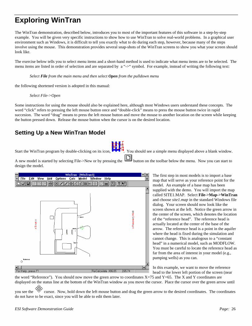
ESI Software Demonstration Guide Page: 26
Exploring WinTran
The WinTran demonstration, described below, introduces you to most of the important features of this software in a step-by-stepexample. You will be given very specific instructions to show how to use WinTran to solve real-world problems. In a graphical userenvironment such as Windows, it is difficult to tell you exactly what to do during each step, however, because many of the stepsinvolve using the mouse. This demonstration provides several snap-shots of the WinTran screens to show you what your screen shouldlook like.
The exercise below tells you to select menu items and a short-hand method is used to indicate what menu items are to be selected. Themenu items are listed in order of selection and are separated by a “->“ symbol. For example, instead of writing the following text:
Select File from the main menu and then select Open from the pulldown menu
the following shortened version is adopted in this manual:
Select File->Open
Some instructions for using the mouse should also be explained here, although most Windows users understand these concepts. Theword “click” refers to pressing the left mouse button once and “double-click” means to press the mouse button twice in rapidsuccesion. The word “drag” means to press the left mouse button and move the mouse to another location on the screen while keepingthe button pressed down. Release the mouse button when the cursor is on the desired location.
Setting Up a New WinTran Model
Start the WinTran program by double-clicking on its icon, . You should see a simple menu displayed above a blank window.
A new model is started by selecting File->New or by pressing the button on the toolbar below the menu. Now you can start todesign the model.
The first step in most models is to import a basemap that will serve as your reference point for themodel. An example of a base map has beensupplied with the demo. You will import the mapcalled SITE1.MAP. Select File->Map->WinTranand choose site1.map in the standard Windows filedialog. Your screen should now look like thescreen shown at the left. Notice the green arrow inthe center of the screen, which denotes the locationof the “reference head”. The reference head isactually located at the center of the base of thearrow. The reference head is a point in the aquiferwhere the head is fixed during the simulation andcannot change. This is analogous to a “constanthead” in a numerical model, such as MODFLOW.You must be careful to locate the reference head asfar from the area of interest in your model (e.g.,pumping wells) as you can.
In this example, we want to move the referencehead to the lower left portion of the screen (near
the word “Reference”). You should now move the green arrow to coordinates X=75 and Y=65. The X and Y coordinates aredisplayed on the status line at the bottom of the WinTran window as you move the cursor. Place the cursor over the green arrow until
you see the cursor. Now, hold down the left mouse button and drag the green arrow to the desired coordinates. The coordinatesdo not have to be exact, since you will be able to edit them later.

ESI Software Demonstration Guide Page: 27
Now, again place the cursor over the reference head (green arrow) and double-click the left mouse button. You will see a dialog thatlists data corresponding to the reference head. Check the coordinates listed in the dialog and make sure the coordinates are close to theones given above. Next, change the hydraulic gradient to 0.01 and the head value to 25. Click on the OK button when you are done.
The next step is to make sure that the aquifer properties are set correctly. Select Edit-> Flow Parameters and make sure that theparameters are set to the values below:
Hydraulic conductivity = 100 ft/dBottom Elevation = 0.0 ftTop Elevation = 100.0 ftReference Head = 25.0 ftGradient = 0.01 ft/ftRecharge = 0.0 ft/dPorosity = 0.2
Note that in the steady-state flow model, WinTran automatically determines whether an aquifer is confined or unconfined. The aquiferis unconfined when the head is below the top of the aquifer and it is confined if the head is above the top of the aquifer. In thisexample, the aquifer is unconfined, so you will make the top of the aquifer very high (e.g., a large distance above the reference headvalue of 25 ft.). Click the OK button to end this dialog.
The previous dialog contained a list of all aquifer properties in the WinTran model. You need to maintain a consistent set of unitswhen you assign these parameters. This is done by selecting one unit of measure for length (e.g. feet) and one unit of measure for time(e.g. days). Using these examples, hydraulic conductivity has units of ft/d and pumping rates are in ft3/d.
Now, edit the transport parameters by selecting Edit->Transport from the menu. Change the longitudinal dispersivity to 30 ft and thetransverse dispersivity to 6 ft. Click the OK button when you are done. Finally, we will change the time-stepping parameters for thetransport simulation. Select Edit->Time Stepping from the menu. Change the number of time steps to 30 and the maximum time stepsize to 100 days. Click the OK button when you are done.
In order to run the transport model, you need either initial concentrations other than zero or a source of contamination in the model.Sources of contaminant can be injection wells, ponds that recharge the aquifer, or linesinks that are injecting water into the aquifer. Inthis example, you will add a well at the point on the map labeled “Source”. Add a well at this location by selecting Add->Well or byclicking the button. Move the cursor to coordinates X=145 and Y=225 and click the left mouse button. The well will be addedwhere the point of the arrow cursor indicates. Next, a dialog box for the well will be displayed; enter a pumping rate of -1 ft3/d (thenegative sign denotes an injection rate) and a concentration of 100. Now, click the OK button. Note that the word “ReCalculate”appears in the status bar. This reminds you that the contours on the screen may not be representative of your current model.
You have now set up the initial WinTran demo model! To see the results, simply select Calc->Recalculate or click the button.You should see a series of contours that are straight lines, representing the uniform regional hydraulic gradient, but there are noconcentration contours. This is because we have not told WinTran to run the transport model yet; only the flow model was simulated.
Before running the transport model, change the contouring options for both the flow model and for the transport model. SelectOptions->Contour->Flow from the menu. Change the minimum contour level to 18.0 ft and the contour interval to 0.5 ft. Also,change the precision value to 1 and click the OK button. A dialog will prompt you to recontour; select YES to perform therecontouring. Next, choose Options->Contour->Transport. We will contour concentrations every 10 time steps (first parameter onthe dialog) with a starting log cycle concentration of 0.01 and 5 contours per log cycle. Unlike flow, where head is computed on aregular contour interval, concentration is contoured using log intervals. Click the OK button when you are done. Finally, selectOptions->Colors and change the concentration contour color to red.
To run transport, select Model->Transport from the menu. Now select Calc->Recalculate and the flow and transport model will run.You will first see the flow model computed, followed by a progress dialog showing the percentage complete for the transportsimulation. In one of the dialogs above, we told WinTran to contour the results every 10 time steps. You also specified a total of 30time steps for the simulation. You should see WinTran contour concentration 3 times for this simulation. At each time step, youshould see the plume grow larger. The final plume is shown below:

ESI Software Demonstration Guide Page: 28
You should also see information displayed on thestatus line at the bottom of the window. The leftside of the status line will show the current timestep number and time value (time from the start ofthe simulation), as well as the mass balance error.This value should be small (0.01 percent in thiscase). To the right, WinTran displays the Pecletand Courant Criteria for the transport simulation.Generally, the Peclet number should be less than 2and the Courant number less than 1. In this case,the Courant number is a bit high, but the massbalance is good (so we will not worry about it forthis demo).
Simulating RemediationThe next step in the demonstration is to add arecovery well to the model. Select Add->Wellfrom the menu or click the button on thetoolbar. Move the cursor to coordinates X=620,Y=225 (near the word “Recovery Well”) and click
the left mouse button. Change the pumping rate to 10,000 ft3/d and click the OK button.
You will now save the concentrations computed atthe end of the last simulation as initialconcentrations for the remediation scenario. Bydefault, WinTran assumes that initial concentrationsare zero everywhere in the aquifer. You mayoverride this default by selecting Calc->Restartfrom the menu. This action saves the currentconcentrations as initial conditions for the next run.Do this now.
To see the results, simply select Calc->Recalculateor click the button. This time, you will see thecone of depression around the recovery well and theconcentration contours stop at the recovery well.Note that the source is still in place, so a steady-stateconcentration distribution develops between thesource and recovery well, as shown in the figure atthe left.
As a final demonstration, we will remove the source
to observe the clean-up of the plume. First, place the cursor over the source well until you see the cursor. Click the left mousebutton to select the well. Now, press the Del key or select Edit->Delete from the menu to remove the well. Select Calc->Restart tosave the previous concentrations as intial conditions and select Calc->Recalculate to see the results. Notice that the plume disappearsquickly. To get a better picture of the cleanup, select Edit->Time Stepping and change the number of time steps to 10 and themaximum time step size to 10. Select Calc->Recalculate and your screen should look like the following:

ESI Software Demonstration Guide Page: 29
.
Concentration Breakthrough Curves
In addition to contours of concentration and head, WinTran can plot concentration over time at observation wells. You defineobservation wells by clicking on the check-box labeled “Monitor Concentration vs. Time” on the well dialog. The next time you runthe model, WinTran will store concentrations computed at all observation wells for all time steps. You plot the results by selectingCalc->Plot C vs. T from the main menu. The following will show you how to create a Concentration vs. Time plot.
First, we will start with our original example. Close the current model by selecting File->Close. Now read in a new model byselecting File->Open. Choose the file called “ex1.wtr” in the file open dialog. Click OK when you have found this file. WinTran willread the file and compute heads only. WinTran does not compute the transport model when you open a new file because thesesimulations can be quite long for complex models.
Before running the transport model, we will define two observation well locations. Select Add->Well from the menu or click the button on the toolbar. Move the cursor to coordinates X=340, Y=230 and click the left mouse button. The coordinates do not need tobe exact. Change the pumping rate to 0.0 and click the check-box labeled “Monitor Concentration vs. Time”. A check mark in thisbox tells WinTran to store concentration information at this well location. Click on the button labeled “Name” and enter a name of“MW1” for this well. Naming the well will allow you to distinguish between multiple observation wells on the plot. The zeropumping rate means that the well is for observation purposes only. You may also monitor concentration vs. time in pumping wells.Click the OK button to end this dialog. Now, repeat this procedure to add an observation well at X=500, Y=230. Call this well MW2.
Select Model->Transport and click the calculator button to run the transport model. When the model is finished running, select Calc->Plot C vs. T from the main menu. A dialog will be displayed that allows you to set up the axes of the graph. Enter the followingnumbers:
Minimum Time 0.0Maximum Time 1000.0Delta T 100.0Number of decimals 0
Minimum Concentration 0.0Maximum Concentration 0.04Delta-C 0.005Number of decimals 3

ESI Software Demonstration Guide Page: 30
Click OK to end editing on this dialog and a plot of concentration versus time is created for the two observation wells. You screenshould look like the one shown below:
We hope that this brief demonstration has shown you what a powerful tool WinTran can be in simulating the fate and transport ofdissolved contaminants in groundwater. If you have any questions or would like to order WinTran, please give us a call.
Scientific Software GroupPO Box 23041Washington, DC 20026-3041Phone: 703-620-9214Fax: 703-620-6793e-mail: [email protected] site: http://www.scisoftware.com