Embed Size (px)
Citation preview

GROMACSUSER
MANUALGroningen Machine for Chemical Simulations
Version 3.1.1

GROMACSUSER MANUAL
Version 3.1.1
David van der SpoelAldert R. van Buuren
Emile ApolPieter J. MeulenhoffD. Peter Tieleman
Alfons L.T.M. SijbersBerk Hess
K. Anton FeenstraErik Lindahl
Rudi van DrunenHerman J.C. Berendsen
c© 1991–2002Department of Biophysical Chemistry, University of Groningen.
Nijenborgh 4, 9747 AG Groningen, The Netherlands.
iv
Preface & Disclaimer
This manual is not complete and has no pretention to be so due to lack of time of the contributors– our first priority is to improve the software. It is meant as a source of information and referencesfor the GROMACS user. It covers both the physical background of MD simulations in general anddetails of the GROMACS software in particular. The manual is continuously being worked on,which in some cases might mean the information is not entirely correct.
When citing this document in any scientific publication please refer to it as:
D. van der Spoel, A. R. van Buuren, E. Apol, P. J. Meulenhoff, D. P. Tieleman,A. L. T. M. Sijbers, B. Hess, K. A. Feenstra, E. Lindahl, R. van Drunen and H. J. C.Berendsen, Gromacs User Manual version 3.1.1, Nijenborgh 4, 9747 AGGroningen, The Netherlands. Internet:www.gromacs.org(2002)
or, if you use BibTeX, you can directly copy the following:
@Manual{gmx31,title = "Gromacs {U}ser {M}anual version 3.1",author = "David van der Spoel and Aldert R. van Buuren and
Emile Apol and Pieter J. Meulen\-hoff and D. PeterTieleman and Alfons L. T. M. Sij\-bers and Berk Hessand K. Anton Feenstra and Erik Lindahl andRudi van Drunen and Herman J. C. Berendsen",
address= "Nij\-enborgh 4, 9747 AG Groningen, The Netherlands.Internet: http://www.gromacs.org",
year = "2001"}
We humbly ask that you cite the GROMACS papers [1, 2] when you publish your results. Anyfuture development depends on academic research grants, since the package is distributed as freesoftware!
Comments are welcome, please send them by e-mail [email protected].
Groningen, April 18, 2002.
Department of Biophysical ChemistryUniversity of GroningenNijenborgh 49747 AG GroningenThe NetherlandsFax: +31-503634800

v
Online Resources
You can find more documentation and other material at our homepagewww.gromacs.org. Amongother things there is an online reference, several GROMACS mailing lists with archives and con-tributed topologies/force fields.
Manual and GROMACS versions
We try to release an updated version of the manual whenever we release a new version of the soft-ware, so in general it is a good idea to use a manual with the same major and minor release numberas your GROMACS installation. Any revision numbers (like 3.1.1) are however independent, tomake it possible to implement bugfixes and manual improvements if necessary.
GROMACS is Free Software
The entire GROMACS package is available under the GNU General Public License. This meansit’s free as in free speech, not just that you can use it without paying us money. For details, checkthe COPYING file in the source code or consultwww.gnu.org/copyleft/gpl.html.
The GROMACS source code and Linux packages are available on our homepage!

vi
Contents
1 Introduction 1
1.1 Computational Chemistry and Molecular Modeling. . . . . . . . . . . . . . . . 1
1.2 Molecular Dynamics Simulations. . . . . . . . . . . . . . . . . . . . . . . . . . 2
1.3 Energy Minimization and Search Methods. . . . . . . . . . . . . . . . . . . . . 5
2 Definitions and Units 7
2.1 Notation. . . . . . . . . . . . . . . . . . . . . . . . . . . . . . . . . . . . . . . 7
2.2 MD units . . . . . . . . . . . . . . . . . . . . . . . . . . . . . . . . . . . . . . 7
2.3 Reduced units. . . . . . . . . . . . . . . . . . . . . . . . . . . . . . . . . . . . 9
3 Algorithms 11
3.1 Introduction. . . . . . . . . . . . . . . . . . . . . . . . . . . . . . . . . . . . . 11
3.2 Periodic boundary conditions. . . . . . . . . . . . . . . . . . . . . . . . . . . . 11
3.2.1 Some useful box types. . . . . . . . . . . . . . . . . . . . . . . . . . . 13
3.2.2 Cutoff restrictions . . . . . . . . . . . . . . . . . . . . . . . . . . . . . 14
3.3 The group concept. . . . . . . . . . . . . . . . . . . . . . . . . . . . . . . . . 14
3.4 Molecular Dynamics. . . . . . . . . . . . . . . . . . . . . . . . . . . . . . . . 15
3.4.1 Initial conditions . . . . . . . . . . . . . . . . . . . . . . . . . . . . . . 15
3.4.2 Neighbor searching. . . . . . . . . . . . . . . . . . . . . . . . . . . . . 18
3.4.3 Compute forces. . . . . . . . . . . . . . . . . . . . . . . . . . . . . . . 20
3.4.4 Update configuration. . . . . . . . . . . . . . . . . . . . . . . . . . . . 21
3.4.5 Temperature coupling. . . . . . . . . . . . . . . . . . . . . . . . . . . 22
3.4.6 Pressure coupling. . . . . . . . . . . . . . . . . . . . . . . . . . . . . . 24
3.4.7 Output step. . . . . . . . . . . . . . . . . . . . . . . . . . . . . . . . . 28
3.5 Shell molecular dynamics. . . . . . . . . . . . . . . . . . . . . . . . . . . . . . 28
3.5.1 Optimization of the shell positions. . . . . . . . . . . . . . . . . . . . . 28
viii Contents
3.6 Constraint algorithms. . . . . . . . . . . . . . . . . . . . . . . . . . . . . . . . 29
3.6.1 SHAKE. . . . . . . . . . . . . . . . . . . . . . . . . . . . . . . . . . . 29
3.6.2 LINCS . . . . . . . . . . . . . . . . . . . . . . . . . . . . . . . . . . . 30
3.7 Simulated Annealing. . . . . . . . . . . . . . . . . . . . . . . . . . . . . . . . 32
3.8 Stochastic Dynamics. . . . . . . . . . . . . . . . . . . . . . . . . . . . . . . . 32
3.9 Brownian Dynamics . . . . . . . . . . . . . . . . . . . . . . . . . . . . . . . . 33
3.10 Energy Minimization. . . . . . . . . . . . . . . . . . . . . . . . . . . . . . . . 33
3.10.1 Steepest Descent. . . . . . . . . . . . . . . . . . . . . . . . . . . . . . 33
3.10.2 Conjugate Gradient. . . . . . . . . . . . . . . . . . . . . . . . . . . . . 34
3.11 Normal Mode Analysis. . . . . . . . . . . . . . . . . . . . . . . . . . . . . . . 34
3.12 Free energy calculations. . . . . . . . . . . . . . . . . . . . . . . . . . . . . . 35
3.13 Essential Dynamics Sampling. . . . . . . . . . . . . . . . . . . . . . . . . . . 37
3.14 Parallelization. . . . . . . . . . . . . . . . . . . . . . . . . . . . . . . . . . . . 38
3.14.1 Methods of parallelization. . . . . . . . . . . . . . . . . . . . . . . . . 38
3.14.2 MD on a ring of processors. . . . . . . . . . . . . . . . . . . . . . . . . 39
3.15 Parallel Molecular Dynamics. . . . . . . . . . . . . . . . . . . . . . . . . . . . 43
3.15.1 Domain decomposition. . . . . . . . . . . . . . . . . . . . . . . . . . . 43
3.15.2 Domain decomposition for non-bonded forces. . . . . . . . . . . . . . . 44
3.15.3 Parallel PPPM. . . . . . . . . . . . . . . . . . . . . . . . . . . . . . . 45
3.15.4 Parallel sorting. . . . . . . . . . . . . . . . . . . . . . . . . . . . . . . 46
4 Force fields 49
4.1 Non-bonded interactions. . . . . . . . . . . . . . . . . . . . . . . . . . . . . . 50
4.1.1 The Lennard-Jones interaction. . . . . . . . . . . . . . . . . . . . . . . 50
4.1.2 Buckingham potential. . . . . . . . . . . . . . . . . . . . . . . . . . . 51
4.1.3 Coulomb interaction. . . . . . . . . . . . . . . . . . . . . . . . . . . . 52
4.1.4 Coulomb interaction with reaction field. . . . . . . . . . . . . . . . . . 52
4.1.5 Modified non-bonded interactions. . . . . . . . . . . . . . . . . . . . . 53
4.1.6 Modified short-range interactions with Ewald summation. . . . . . . . . 55
4.2 Bonded interactions. . . . . . . . . . . . . . . . . . . . . . . . . . . . . . . . . 56
4.2.1 Bond stretching. . . . . . . . . . . . . . . . . . . . . . . . . . . . . . . 56
4.2.2 Morse potential bond stretching. . . . . . . . . . . . . . . . . . . . . . 57
4.2.3 Cubic bond stretching potential. . . . . . . . . . . . . . . . . . . . . . 58
4.2.4 Harmonic angle potential. . . . . . . . . . . . . . . . . . . . . . . . . . 58
Contents ix
4.2.5 Cosine based angle potential. . . . . . . . . . . . . . . . . . . . . . . . 59
4.2.6 Improper dihedrals. . . . . . . . . . . . . . . . . . . . . . . . . . . . . 59
4.2.7 Proper dihedrals. . . . . . . . . . . . . . . . . . . . . . . . . . . . . . 59
4.2.8 Special interactions. . . . . . . . . . . . . . . . . . . . . . . . . . . . . 62
4.2.9 Position restraints. . . . . . . . . . . . . . . . . . . . . . . . . . . . . . 63
4.2.10 Angle restraints. . . . . . . . . . . . . . . . . . . . . . . . . . . . . . . 64
4.2.11 Distance restraints. . . . . . . . . . . . . . . . . . . . . . . . . . . . . 64
4.2.12 Orientation restraints. . . . . . . . . . . . . . . . . . . . . . . . . . . . 68
4.3 Free energy interactions. . . . . . . . . . . . . . . . . . . . . . . . . . . . . . . 71
4.3.1 Soft-core interactions. . . . . . . . . . . . . . . . . . . . . . . . . . . . 74
4.4 Methods. . . . . . . . . . . . . . . . . . . . . . . . . . . . . . . . . . . . . . . 75
4.4.1 Exclusions and 1-4 Interactions.. . . . . . . . . . . . . . . . . . . . . . 75
4.4.2 Charge Groups.. . . . . . . . . . . . . . . . . . . . . . . . . . . . . . . 75
4.4.3 Treatment of cutoffs. . . . . . . . . . . . . . . . . . . . . . . . . . . . 76
4.5 Dummy atoms. . . . . . . . . . . . . . . . . . . . . . . . . . . . . . . . . . . . 76
4.6 Long Range Electrostatics. . . . . . . . . . . . . . . . . . . . . . . . . . . . . 80
4.6.1 Ewald summation. . . . . . . . . . . . . . . . . . . . . . . . . . . . . . 80
4.6.2 PME . . . . . . . . . . . . . . . . . . . . . . . . . . . . . . . . . . . . 81
4.6.3 PPPM. . . . . . . . . . . . . . . . . . . . . . . . . . . . . . . . . . . . 81
4.6.4 Optimizing Fourier transforms. . . . . . . . . . . . . . . . . . . . . . . 82
4.7 All-hydrogen force-field . . . . . . . . . . . . . . . . . . . . . . . . . . . . . . 83
4.8 GROMOS-96 notes. . . . . . . . . . . . . . . . . . . . . . . . . . . . . . . . . 83
4.8.1 The GROMOS-96 force field. . . . . . . . . . . . . . . . . . . . . . . . 83
4.8.2 GROMOS-96 files. . . . . . . . . . . . . . . . . . . . . . . . . . . . . 84
5 Topologies 85
5.1 Introduction. . . . . . . . . . . . . . . . . . . . . . . . . . . . . . . . . . . . . 85
5.2 Particle type. . . . . . . . . . . . . . . . . . . . . . . . . . . . . . . . . . . . . 85
5.2.1 Atom types. . . . . . . . . . . . . . . . . . . . . . . . . . . . . . . . . 86
5.2.2 Dummy atoms. . . . . . . . . . . . . . . . . . . . . . . . . . . . . . . 87
5.3 Parameter files . . . . . . . . . . . . . . . . . . . . . . . . . . . . . . . . . . . 88
5.3.1 Atoms. . . . . . . . . . . . . . . . . . . . . . . . . . . . . . . . . . . . 88
5.3.2 Bonded parameters. . . . . . . . . . . . . . . . . . . . . . . . . . . . . 89
5.3.3 Non-bonded parameters. . . . . . . . . . . . . . . . . . . . . . . . . . 90
x Contents
5.3.4 Pair interactions . . . . . . . . . . . . . . . . . . . . . . . . . . . . . . 91
5.3.5 Exclusions . . . . . . . . . . . . . . . . . . . . . . . . . . . . . . . . . 91
5.4 Constraints . . . . . . . . . . . . . . . . . . . . . . . . . . . . . . . . . . . . . 92
5.5 Databases. . . . . . . . . . . . . . . . . . . . . . . . . . . . . . . . . . . . . . 92
5.5.1 Residue database. . . . . . . . . . . . . . . . . . . . . . . . . . . . . . 92
5.5.2 Hydrogen database. . . . . . . . . . . . . . . . . . . . . . . . . . . . . 94
5.5.3 Termini database. . . . . . . . . . . . . . . . . . . . . . . . . . . . . . 96
5.6 File formats . . . . . . . . . . . . . . . . . . . . . . . . . . . . . . . . . . . . . 97
5.6.1 Topology file . . . . . . . . . . . . . . . . . . . . . . . . . . . . . . . . 97
5.6.2 Molecule.itp file . . . . . . . . . . . . . . . . . . . . . . . . . . . . . . 103
5.6.3 Ifdef option. . . . . . . . . . . . . . . . . . . . . . . . . . . . . . . . .104
5.6.4 Free energy calculations. . . . . . . . . . . . . . . . . . . . . . . . . . 105
5.6.5 Constraint force. . . . . . . . . . . . . . . . . . . . . . . . . . . . . . .107
5.6.6 Coordinate file. . . . . . . . . . . . . . . . . . . . . . . . . . . . . . .108
5.7 Force-field organization . . . . . . . . . . . . . . . . . . . . . . . . . . . . . . 108
5.7.1 Force-field files. . . . . . . . . . . . . . . . . . . . . . . . . . . . . . .108
5.7.2 Changing force-field parameters. . . . . . . . . . . . . . . . . . . . . . 109
5.7.3 Adding atom types. . . . . . . . . . . . . . . . . . . . . . . . . . . . . 110
6 Special Topics 111
6.1 Calculating potentials of mean force: the pull code. . . . . . . . . . . . . . . . 111
6.1.1 Overview . . . . . . . . . . . . . . . . . . . . . . . . . . . . . . . . . .111
6.1.2 Usage. . . . . . . . . . . . . . . . . . . . . . . . . . . . . . . . . . . .112
6.1.3 Output . . . . . . . . . . . . . . . . . . . . . . . . . . . . . . . . . . .115
6.1.4 Limitations . . . . . . . . . . . . . . . . . . . . . . . . . . . . . . . . .115
6.1.5 Implementation. . . . . . . . . . . . . . . . . . . . . . . . . . . . . . .116
6.1.6 Future development. . . . . . . . . . . . . . . . . . . . . . . . . . . . . 116
6.2 Removing fastest degrees of freedom. . . . . . . . . . . . . . . . . . . . . . . . 116
6.2.1 Hydrogen bond-angle vibrations. . . . . . . . . . . . . . . . . . . . . . 117
6.2.2 Out-of-plane vibrations in aromatic groups. . . . . . . . . . . . . . . . 118
6.3 Viscosity calculation . . . . . . . . . . . . . . . . . . . . . . . . . . . . . . . .119
6.4 Tabulated functions. . . . . . . . . . . . . . . . . . . . . . . . . . . . . . . . .121
6.4.1 Cubic splines for potentials. . . . . . . . . . . . . . . . . . . . . . . . . 121
6.4.2 User specified potential functions. . . . . . . . . . . . . . . . . . . . . 122
Contents xi
7 Run parameters and Programs 125
7.1 Online and html manuals. . . . . . . . . . . . . . . . . . . . . . . . . . . . . . 125
7.2 File types . . . . . . . . . . . . . . . . . . . . . . . . . . . . . . . . . . . . . .125
7.3 Run Parameters. . . . . . . . . . . . . . . . . . . . . . . . . . . . . . . . . . .127
7.3.1 General. . . . . . . . . . . . . . . . . . . . . . . . . . . . . . . . . . .127
7.3.2 Preprocessing. . . . . . . . . . . . . . . . . . . . . . . . . . . . . . . .127
7.3.3 Run control. . . . . . . . . . . . . . . . . . . . . . . . . . . . . . . . .127
7.3.4 Langevin dynamics. . . . . . . . . . . . . . . . . . . . . . . . . . . . . 129
7.3.5 Energy minimization. . . . . . . . . . . . . . . . . . . . . . . . . . . . 129
7.3.6 Shell Molecular Dynamics. . . . . . . . . . . . . . . . . . . . . . . . . 129
7.3.7 Output control . . . . . . . . . . . . . . . . . . . . . . . . . . . . . . .129
7.3.8 Neighbor searching. . . . . . . . . . . . . . . . . . . . . . . . . . . . . 130
7.3.9 Electrostatics and VdW. . . . . . . . . . . . . . . . . . . . . . . . . . . 131
7.3.10 Temperature coupling. . . . . . . . . . . . . . . . . . . . . . . . . . . 133
7.3.11 Pressure coupling. . . . . . . . . . . . . . . . . . . . . . . . . . . . . . 134
7.3.12 Simulated annealing. . . . . . . . . . . . . . . . . . . . . . . . . . . . 135
7.3.13 Velocity generation. . . . . . . . . . . . . . . . . . . . . . . . . . . . . 136
7.3.14 Bonds. . . . . . . . . . . . . . . . . . . . . . . . . . . . . . . . . . . .136
7.3.15 Energy group exclusions. . . . . . . . . . . . . . . . . . . . . . . . . . 137
7.3.16 NMR refinement. . . . . . . . . . . . . . . . . . . . . . . . . . . . . . 138
7.3.17 Free Energy Perturbation. . . . . . . . . . . . . . . . . . . . . . . . . . 139
7.3.18 Non-equilibrium MD. . . . . . . . . . . . . . . . . . . . . . . . . . . . 139
7.3.19 Electric fields. . . . . . . . . . . . . . . . . . . . . . . . . . . . . . . .140
7.3.20 User defined thingies. . . . . . . . . . . . . . . . . . . . . . . . . . . . 140
7.4 Programs by topic. . . . . . . . . . . . . . . . . . . . . . . . . . . . . . . . . .140
8 Analysis 145
8.1 Groups in Analysis.. . . . . . . . . . . . . . . . . . . . . . . . . . . . . . . . .145
8.1.1 Default Groups. . . . . . . . . . . . . . . . . . . . . . . . . . . . . . .146
8.2 Looking at your trajectory . . . . . . . . . . . . . . . . . . . . . . . . . . . . . 147
8.3 General properties. . . . . . . . . . . . . . . . . . . . . . . . . . . . . . . . . .147
8.4 Radial distribution functions. . . . . . . . . . . . . . . . . . . . . . . . . . . . 148
8.5 Correlation functions. . . . . . . . . . . . . . . . . . . . . . . . . . . . . . . .149
8.5.1 Theory of correlation functions. . . . . . . . . . . . . . . . . . . . . . 149
xii Contents
8.5.2 Using FFT for computation of the ACF. . . . . . . . . . . . . . . . . . 151
8.5.3 Special forms of the ACF. . . . . . . . . . . . . . . . . . . . . . . . . . 151
8.5.4 Some Applications. . . . . . . . . . . . . . . . . . . . . . . . . . . . . 151
8.5.5 Mean Square Displacement. . . . . . . . . . . . . . . . . . . . . . . . 152
8.6 Bonds, angles and dihedrals. . . . . . . . . . . . . . . . . . . . . . . . . . . . 152
8.7 Radius of gyration and distances. . . . . . . . . . . . . . . . . . . . . . . . . . 155
8.8 Root mean square deviations in structure. . . . . . . . . . . . . . . . . . . . . . 156
8.9 Covariance analysis. . . . . . . . . . . . . . . . . . . . . . . . . . . . . . . . .157
8.10 Hydrogen bonds. . . . . . . . . . . . . . . . . . . . . . . . . . . . . . . . . . .158
8.11 Protein related items. . . . . . . . . . . . . . . . . . . . . . . . . . . . . . . .160
8.12 Interface related items. . . . . . . . . . . . . . . . . . . . . . . . . . . . . . . .162
8.13 Chemical shifts. . . . . . . . . . . . . . . . . . . . . . . . . . . . . . . . . . .163
A Technical Details 165
A.1 Installation . . . . . . . . . . . . . . . . . . . . . . . . . . . . . . . . . . . . .165
A.2 Single or Double precision. . . . . . . . . . . . . . . . . . . . . . . . . . . . . 165
A.3 Porting GROMACS. . . . . . . . . . . . . . . . . . . . . . . . . . . . . . . . .166
A.3.1 Multi-processor Optimization. . . . . . . . . . . . . . . . . . . . . . . 167
A.4 Environment Variables. . . . . . . . . . . . . . . . . . . . . . . . . . . . . . .167
A.5 Running GROMACS in parallel . . . . . . . . . . . . . . . . . . . . . . . . . . 168
B Some implementation details 171
B.1 Single Sum Virial in GROMACS. . . . . . . . . . . . . . . . . . . . . . . . . . 171
B.1.1 Virial. . . . . . . . . . . . . . . . . . . . . . . . . . . . . . . . . . . . .171
B.1.2 Virial from non-bonded forces.. . . . . . . . . . . . . . . . . . . . . . . 172
B.1.3 The intramolecular shift (mol-shift).. . . . . . . . . . . . . . . . . . . . 172
B.1.4 Virial from Covalent Bonds.. . . . . . . . . . . . . . . . . . . . . . . . 173
B.1.5 Virial from Shake. . . . . . . . . . . . . . . . . . . . . . . . . . . . . . 174
B.2 Optimizations. . . . . . . . . . . . . . . . . . . . . . . . . . . . . . . . . . . .174
B.2.1 Inner Loops for Water. . . . . . . . . . . . . . . . . . . . . . . . . . . 174
B.2.2 Fortran Code. . . . . . . . . . . . . . . . . . . . . . . . . . . . . . . .175
B.3 Computation of the 1.0/sqrt function.. . . . . . . . . . . . . . . . . . . . . . . . 175
B.3.1 Introduction. . . . . . . . . . . . . . . . . . . . . . . . . . . . . . . . .175
B.3.2 General. . . . . . . . . . . . . . . . . . . . . . . . . . . . . . . . . . .175
B.3.3 Applied to floating point numbers. . . . . . . . . . . . . . . . . . . . . 176
Contents xiii
B.3.4 Specification of the lookup table. . . . . . . . . . . . . . . . . . . . . . 177
B.3.5 Separate exponent and fraction computation. . . . . . . . . . . . . . . . 178
B.3.6 Implementation. . . . . . . . . . . . . . . . . . . . . . . . . . . . . . .179
C Long range corrections 181
C.1 Dispersion. . . . . . . . . . . . . . . . . . . . . . . . . . . . . . . . . . . . . .181
C.1.1 Energy . . . . . . . . . . . . . . . . . . . . . . . . . . . . . . . . . . .181
C.1.2 Virial and pressure. . . . . . . . . . . . . . . . . . . . . . . . . . . . . 182
D Averages and fluctuations 185
D.1 Formulae for averaging. . . . . . . . . . . . . . . . . . . . . . . . . . . . . . .185
D.2 Implementation. . . . . . . . . . . . . . . . . . . . . . . . . . . . . . . . . . .186
D.2.1 Part of a Simulation . . . . . . . . . . . . . . . . . . . . . . . . . . . . 187
D.2.2 Combining two simulations. . . . . . . . . . . . . . . . . . . . . . . . 187
D.2.3 Summing energy terms. . . . . . . . . . . . . . . . . . . . . . . . . . . 188
E Manual Pages 191
E.1 options. . . . . . . . . . . . . . . . . . . . . . . . . . . . . . . . . . . . . . . .191
E.2 dodssp . . . . . . . . . . . . . . . . . . . . . . . . . . . . . . . . . . . . . . .192
E.3 editconf . . . . . . . . . . . . . . . . . . . . . . . . . . . . . . . . . . . . . . .193
E.4 eneconv. . . . . . . . . . . . . . . . . . . . . . . . . . . . . . . . . . . . . . .194
E.5 ffscan . . . . . . . . . . . . . . . . . . . . . . . . . . . . . . . . . . . . . . . .195
E.6 g anaeig. . . . . . . . . . . . . . . . . . . . . . . . . . . . . . . . . . . . . . .195
E.7 g analyze . . . . . . . . . . . . . . . . . . . . . . . . . . . . . . . . . . . . . .197
E.8 g angle . . . . . . . . . . . . . . . . . . . . . . . . . . . . . . . . . . . . . . .198
E.9 g bond. . . . . . . . . . . . . . . . . . . . . . . . . . . . . . . . . . . . . . . .199
E.10 gbundle. . . . . . . . . . . . . . . . . . . . . . . . . . . . . . . . . . . . . . .200
E.11 gchi . . . . . . . . . . . . . . . . . . . . . . . . . . . . . . . . . . . . . . . . .201
E.12 gcluster . . . . . . . . . . . . . . . . . . . . . . . . . . . . . . . . . . . . . . .202
E.13 gclustsize. . . . . . . . . . . . . . . . . . . . . . . . . . . . . . . . . . . . . .203
E.14 gconfrms . . . . . . . . . . . . . . . . . . . . . . . . . . . . . . . . . . . . . .204
E.15 gcovar . . . . . . . . . . . . . . . . . . . . . . . . . . . . . . . . . . . . . . .204
E.16 gdensity . . . . . . . . . . . . . . . . . . . . . . . . . . . . . . . . . . . . . .205
E.17 gdielectric . . . . . . . . . . . . . . . . . . . . . . . . . . . . . . . . . . . . .206
E.18 gdih . . . . . . . . . . . . . . . . . . . . . . . . . . . . . . . . . . . . . . . . .207
xiv Contents
E.19 gdipoles . . . . . . . . . . . . . . . . . . . . . . . . . . . . . . . . . . . . . .207
E.20 gdisre . . . . . . . . . . . . . . . . . . . . . . . . . . . . . . . . . . . . . . . .209
E.21 gdist . . . . . . . . . . . . . . . . . . . . . . . . . . . . . . . . . . . . . . . .209
E.22 gdyndom . . . . . . . . . . . . . . . . . . . . . . . . . . . . . . . . . . . . . .210
E.23 genbox. . . . . . . . . . . . . . . . . . . . . . . . . . . . . . . . . . . . . . . .210
E.24 genconf . . . . . . . . . . . . . . . . . . . . . . . . . . . . . . . . . . . . . . .211
E.25 genemat . . . . . . . . . . . . . . . . . . . . . . . . . . . . . . . . . . . . . .212
E.26 genergy. . . . . . . . . . . . . . . . . . . . . . . . . . . . . . . . . . . . . . .213
E.27 genion. . . . . . . . . . . . . . . . . . . . . . . . . . . . . . . . . . . . . . . .214
E.28 genpr . . . . . . . . . . . . . . . . . . . . . . . . . . . . . . . . . . . . . . . .215
E.29 ggyrate . . . . . . . . . . . . . . . . . . . . . . . . . . . . . . . . . . . . . . .215
E.30 gh2order . . . . . . . . . . . . . . . . . . . . . . . . . . . . . . . . . . . . . .216
E.31 ghbond . . . . . . . . . . . . . . . . . . . . . . . . . . . . . . . . . . . . . . .216
E.32 ghelix . . . . . . . . . . . . . . . . . . . . . . . . . . . . . . . . . . . . . . . .218
E.33 glie . . . . . . . . . . . . . . . . . . . . . . . . . . . . . . . . . . . . . . . . .219
E.34 gmdmat. . . . . . . . . . . . . . . . . . . . . . . . . . . . . . . . . . . . . . .219
E.35 gmindist . . . . . . . . . . . . . . . . . . . . . . . . . . . . . . . . . . . . . .220
E.36 gmorph . . . . . . . . . . . . . . . . . . . . . . . . . . . . . . . . . . . . . . .220
E.37 gmsd . . . . . . . . . . . . . . . . . . . . . . . . . . . . . . . . . . . . . . . .221
E.38 gmxcheck. . . . . . . . . . . . . . . . . . . . . . . . . . . . . . . . . . . . . .221
E.39 gmxdump. . . . . . . . . . . . . . . . . . . . . . . . . . . . . . . . . . . . . .222
E.40 gnmeig . . . . . . . . . . . . . . . . . . . . . . . . . . . . . . . . . . . . . . .222
E.41 gnmens. . . . . . . . . . . . . . . . . . . . . . . . . . . . . . . . . . . . . . .223
E.42 gorder . . . . . . . . . . . . . . . . . . . . . . . . . . . . . . . . . . . . . . .223
E.43 gpotential. . . . . . . . . . . . . . . . . . . . . . . . . . . . . . . . . . . . . .224
E.44 grama. . . . . . . . . . . . . . . . . . . . . . . . . . . . . . . . . . . . . . . .225
E.45 grdf . . . . . . . . . . . . . . . . . . . . . . . . . . . . . . . . . . . . . . . . .225
E.46 grms . . . . . . . . . . . . . . . . . . . . . . . . . . . . . . . . . . . . . . . .226
E.47 grmsdist . . . . . . . . . . . . . . . . . . . . . . . . . . . . . . . . . . . . . .227
E.48 grmsf . . . . . . . . . . . . . . . . . . . . . . . . . . . . . . . . . . . . . . . .228
E.49 grompp . . . . . . . . . . . . . . . . . . . . . . . . . . . . . . . . . . . . . . .229
E.50 grotacf . . . . . . . . . . . . . . . . . . . . . . . . . . . . . . . . . . . . . . .230
E.51 gsaltbr . . . . . . . . . . . . . . . . . . . . . . . . . . . . . . . . . . . . . . .231
E.52 gsas. . . . . . . . . . . . . . . . . . . . . . . . . . . . . . . . . . . . . . . . .231

Contents xv
E.53 gsgangle . . . . . . . . . . . . . . . . . . . . . . . . . . . . . . . . . . . . . .232
E.54 gsorient. . . . . . . . . . . . . . . . . . . . . . . . . . . . . . . . . . . . . . .233
E.55 gtcaf . . . . . . . . . . . . . . . . . . . . . . . . . . . . . . . . . . . . . . . .233
E.56 gtraj . . . . . . . . . . . . . . . . . . . . . . . . . . . . . . . . . . . . . . . . .234
E.57 gvelacc . . . . . . . . . . . . . . . . . . . . . . . . . . . . . . . . . . . . . . .235
E.58 highway. . . . . . . . . . . . . . . . . . . . . . . . . . . . . . . . . . . . . . .236
E.59 makendx . . . . . . . . . . . . . . . . . . . . . . . . . . . . . . . . . . . . . .236
E.60 mdrun . . . . . . . . . . . . . . . . . . . . . . . . . . . . . . . . . . . . . . . .237
E.61 mkangndx . . . . . . . . . . . . . . . . . . . . . . . . . . . . . . . . . . . . .238
E.62 ngmx . . . . . . . . . . . . . . . . . . . . . . . . . . . . . . . . . . . . . . . .238
E.63 pdb2gmx . . . . . . . . . . . . . . . . . . . . . . . . . . . . . . . . . . . . . .239
E.64 protonate . . . . . . . . . . . . . . . . . . . . . . . . . . . . . . . . . . . . . .240
E.65 tpbconv . . . . . . . . . . . . . . . . . . . . . . . . . . . . . . . . . . . . . . .241
E.66 trjcat. . . . . . . . . . . . . . . . . . . . . . . . . . . . . . . . . . . . . . . . .241
E.67 trjconv. . . . . . . . . . . . . . . . . . . . . . . . . . . . . . . . . . . . . . . .242
E.68 trjorder . . . . . . . . . . . . . . . . . . . . . . . . . . . . . . . . . . . . . . .244
E.69 wheel . . . . . . . . . . . . . . . . . . . . . . . . . . . . . . . . . . . . . . . .244
E.70 x2top . . . . . . . . . . . . . . . . . . . . . . . . . . . . . . . . . . . . . . . .245
E.71 xpm2ps . . . . . . . . . . . . . . . . . . . . . . . . . . . . . . . . . . . . . . .245
E.72 xrama . . . . . . . . . . . . . . . . . . . . . . . . . . . . . . . . . . . . . . . .246
Bibliography 249
Index 255

xvi Contents
Chapter 1
Introduction
1.1 Computational Chemistry and Molecular Modeling
GROMACS is an engine to perform molecular dynamics simulations and energy minimization.These are two of the many techniques that belong to the realm of computational chemistry andmolecular modeling.Computational Chemistryis just a name to indicate the use of computationaltechniques in chemistry, ranging from quantum mechanics of molecules to dynamics of largecomplex molecular aggregates.Molecular modelingindicates the general process of describingcomplex chemical systems in terms of a realistic atomic model, with the aim to understand andpredict macroscopic properties based on detailed knowledge on an atomic scale. Often molecularmodeling is used to design new materials, for which the accurate prediction of physical propertiesof realistic systems is required.
Macroscopic physical properties can be distinguished in (a) static equilibrium properties, such asthe binding constant of an inhibitor to an enzyme, the average potential energy of a system, orthe radial distribution function in a liquid, and (b) dynamic or non-equilibrium properties, suchas the viscosity of a liquid, diffusion processes in membranes, the dynamics of phase changes,reaction kinetics, or the dynamics of defects in crystals. The choice of technique depends on thequestion asked and on the feasibility of the method to yield reliable results at the present state ofthe art. Ideally, the (relativistic) time-dependent Schrodinger equation describes the properties ofmolecular systems with high accuracy, but anything more complex than the equilibrium state of afew atoms cannot be handled at thisab initio level. Thus approximations are necessary; the higherthe complexity of a system and the longer the time span of the processes of interest is, the moresevere the required approximations are. At a certain point (reached very much earlier than onewould wish) theab initio approach must be augmented or replaced byempiricalparameterizationof the model used. Where simulations based on physical principles of atomic interactions still faildue to the complexity of the system (as is unfortunately still the case for the prediction of proteinfolding; but: there is hope!) molecular modeling is based entirely on a similarity analysis of knownstructural and chemical data. The QSAR methods (Quantitative Structure-Activity Relations) andmany homology-based protein structure predictions belong to the latter category.
Macroscopic properties are always ensemble averages over a representative statistical ensemble

2 Chapter 1. Introduction
(either equilibrium or non-equilibrium) of molecular systems. For molecular modeling this hastwo important consequences:
• The knowledge of a single structure, even if it is the structure of the global energy min-imum, is not sufficient. It is necessary to generate a representative ensemble at a giventemperature, in order to compute macroscopic properties. But this is not enough to computethermodynamic equilibrium properties that are based on free energies, such as phase equi-libria, binding constants, solubilities, relative stability of molecular conformations, etc. Thecomputation of free energies and thermodynamic potentials requires special extensions ofmolecular simulation techniques.
• While molecular simulations in principle provide atomic details of the structures and mo-tions, such details are often not relevant for the macroscopic properties of interest. Thisopens the way to simplify the description of interactions and average over irrelevant details.The science of statistical mechanics provides the theoretical framework for such simpli-fications. There is a hierarchy of methods ranging from considering groups of atoms asone unit, describing motion in a reduced number of collective coordinates, averaging oversolvent molecules with potentials of mean force combined with stochastic dynamics [3],to mesoscopic dynamicsdescribing densities rather than atoms and fluxes as response tothermodynamic gradients rather than velocities or accelerations as response to forces [4].
For the generation of a representative equilibrium ensemble two methods are available: (a) MonteCarlo simulationsand (b) Molecular Dynamics simulations. For the generation of non-equilibriumensembles and for the analysis of dynamic events, only the second method is appropriate. WhileMonte Carlo simulations are more simple than MD (they do not require the computation of forces),they do not yield significantly better statistics than MD in a given amount of computer time. There-fore MD is the more universal technique. If a starting configuration is very far from equilibrium,the forces may be excessively large and the MD simulation may fail. In those cases a robusten-ergy minimizationis required. Another reason to perform an energy minimization is the removalof all kinetic energy from the system: if several ’snapshots’ from dynamic simulations must becompared, energy minimization reduces the thermal noise in the structures and potential energies,so that they can be compared better.
1.2 Molecular Dynamics Simulations
MD simulations solve Newton’s equations of motion for a system ofN interacting atoms:
mi∂2ri
∂t2= F i, i = 1 . . . N. (1.1)
The forces are the negative derivatives of a potential functionV (r1, r2, . . . , rN ):
F i = −∂V∂ri
(1.2)
The equations are solved simultaneously in small time steps. The system is followed for sometime, taking care that the temperature and pressure remain at the required values, and the coor-dinates are written to an output file at regular intervals. The coordinates as a function of time
1.2. Molecular Dynamics Simulations 3
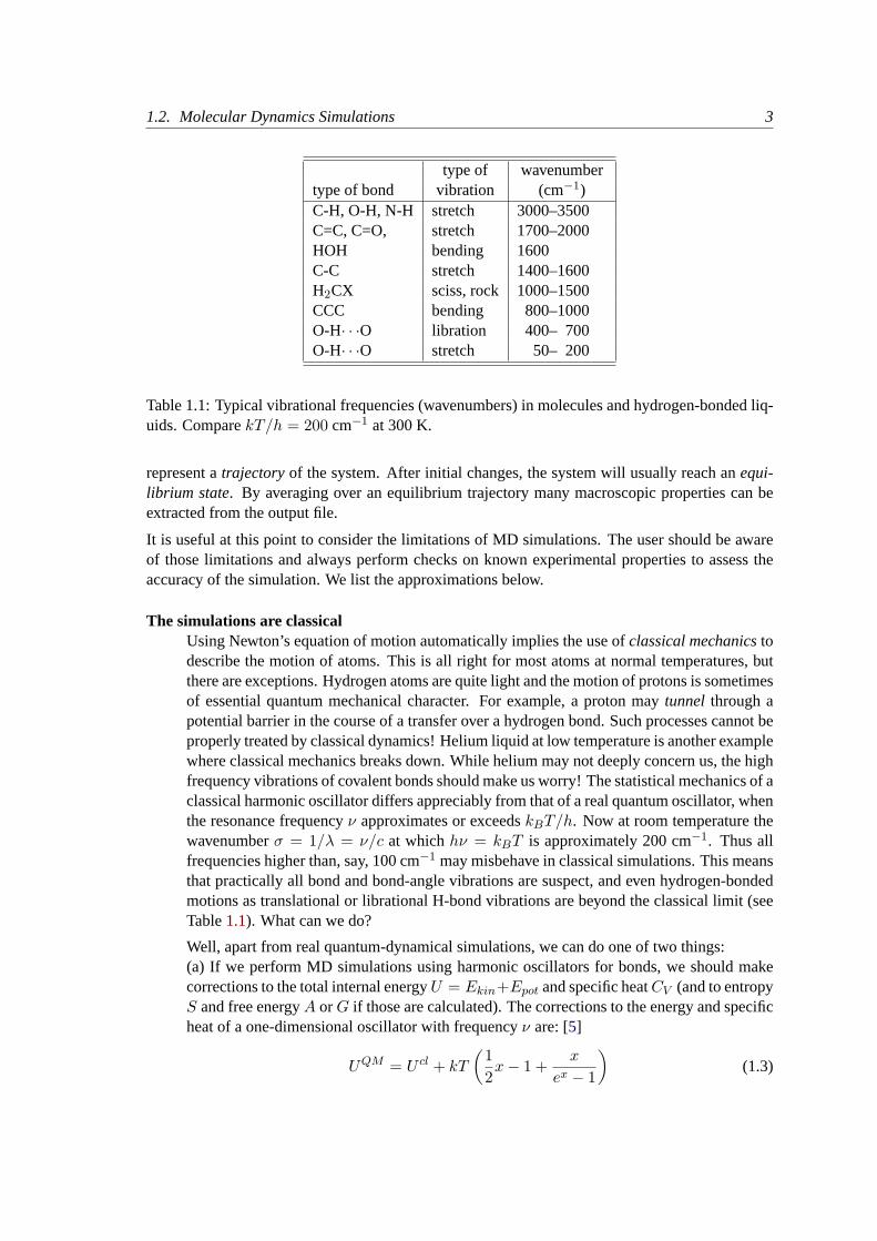
type of wavenumbertype of bond vibration (cm−1)C-H, O-H, N-H stretch 3000–3500C=C, C=O, stretch 1700–2000HOH bending 1600C-C stretch 1400–1600H2CX sciss, rock 1000–1500CCC bending 800–1000O-H· · ·O libration 400– 700O-H· · ·O stretch 50– 200
Table 1.1: Typical vibrational frequencies (wavenumbers) in molecules and hydrogen-bonded liq-uids. ComparekT/h = 200 cm−1 at 300 K.
represent atrajectoryof the system. After initial changes, the system will usually reach anequi-librium state. By averaging over an equilibrium trajectory many macroscopic properties can beextracted from the output file.
It is useful at this point to consider the limitations of MD simulations. The user should be awareof those limitations and always perform checks on known experimental properties to assess theaccuracy of the simulation. We list the approximations below.
The simulations are classicalUsing Newton’s equation of motion automatically implies the use ofclassical mechanicstodescribe the motion of atoms. This is all right for most atoms at normal temperatures, butthere are exceptions. Hydrogen atoms are quite light and the motion of protons is sometimesof essential quantum mechanical character. For example, a proton maytunnel through apotential barrier in the course of a transfer over a hydrogen bond. Such processes cannot beproperly treated by classical dynamics! Helium liquid at low temperature is another examplewhere classical mechanics breaks down. While helium may not deeply concern us, the highfrequency vibrations of covalent bonds should make us worry! The statistical mechanics of aclassical harmonic oscillator differs appreciably from that of a real quantum oscillator, whenthe resonance frequencyν approximates or exceedskBT/h. Now at room temperature thewavenumberσ = 1/λ = ν/c at whichhν = kBT is approximately 200 cm−1. Thus allfrequencies higher than, say, 100 cm−1 may misbehave in classical simulations. This meansthat practically all bond and bond-angle vibrations are suspect, and even hydrogen-bondedmotions as translational or librational H-bond vibrations are beyond the classical limit (seeTable1.1). What can we do?
Well, apart from real quantum-dynamical simulations, we can do one of two things:(a) If we perform MD simulations using harmonic oscillators for bonds, we should makecorrections to the total internal energyU = Ekin+Epot and specific heatCV (and to entropyS and free energyA orG if those are calculated). The corrections to the energy and specificheat of a one-dimensional oscillator with frequencyν are: [5]
UQM = U cl + kT
(12x− 1 +
x
ex − 1
)(1.3)
4 Chapter 1. Introduction
CQMV = Ccl
V + k
(x2ex
(ex − 1)2− 1
), (1.4)
wherex = hν/kT . The classical oscillator absorbs too much energy (kT ), while the high-frequency quantum oscillator is in its ground state at the zero-point energy level of1
2hν.(b) We can treat the bonds (and bond angles) asconstraintsin the equation of motion. Therational behind this is that a quantum oscillator in its ground state resembles a constrainedbond more closely than a classical oscillator. A good practical reason for this choice isthat the algorithm can use larger time steps when the highest frequencies are removed. Inpractice the time step can be made four times as large when bonds are constrained thanwhen they are oscillators [6]. GROMACS has this option for the bonds and bond angles.The flexibility of the latter is rather essential to allow for the realistic motion and coverageof configurational space [6].
Electrons are in the ground stateIn MD we use aconservativeforce field that is a function of the positions of atoms only.This means that the electronic motions are not considered: the electrons are supposed toadjust their dynamics instantly when the atomic positions change (theBorn-Oppenheimerapproximation), and remain in their ground state. This is really all right, almost always. Butof course, electron transfer processes and electronically excited states can not be treated.Neither can chemical reactions be treated properly, but there are other reasons to shy awayfrom reactions for the time being.
Force fields are approximateForce fields provide the forces. They are not really a part of the simulation method and theirparameters can be user-modified as the need arises or knowledge improves. But the formof the forces that can be used in a particular program is subject to limitations. The forcefield that is incorporated in GROMACS is described in Chapter 4. In the present versionthe force field is pair-additive (apart from long-range coulomb forces), it cannot incorporatepolarizabilities, and it does not contain fine-tuning of bonded interactions. This urges theinclusion of some limitations in this list below. For the rest it is quite useful and fairlyreliable for bio macro-molecules in aqueous solution!
The force field is pair-additiveThis means that allnon-bondedforces result from the sum of non-bonded pair interactions.Non pair-additive interactions, the most important example of which is interaction throughatomic polarizability, are represented byeffective pair potentials. Only average non pair-additive contributions are incorporated. This also means that the pair interactions are notpure,i.e., they are not valid for isolated pairs or for situations that differ appreciably from thetest systems on which the models were parameterized. In fact, the effective pair potentialsare not that bad in practice. But the omission of polarizability also means that electrons inatoms do not provide a dielectric constant as they should. For example, real liquid alkaneshave a dielectric constant of slightly more than 2, which reduce the long-range electrostaticinteraction between (partial) charges. Thus the simulations will exaggerate the long-rangeCoulomb terms. Luckily, the next item compensates this effect a bit.
Long-range interactions are cutoffIn this version GROMACS always uses a cutoff radius for the Lennard-Jones interactions
1.3. Energy Minimization and Search Methods 5
and sometimes for the Coulomb interactions as well. Due to the minimum-image convention(only one image of each particle in the periodic boundary conditions is considered for a pairinteraction), the cutoff range can not exceed half the box size. That is still pretty big forlarge systems, and trouble is only expected for systems containing charged particles. Butthen truly bad things can happen, like accumulation of charges at the cutoff boundary orvery wrong energies! For such systems you should consider using one of the implementedlong-range electrostatic algorithms.
Boundary conditions are unnaturalSince system size is small (even 10,000 particles is small), a cluster of particles will have alot of unwanted boundary with its environment (vacuum). This we must avoid if we wishto simulate a bulk system. So we use periodic boundary conditions, to avoid real phaseboundaries. But liquids are not crystals, so something unnatural remains. This item ismentioned last because it is the least of the evils. For large systems the errors are small,but for small systems with a lot of internal spatial correlation, the periodic boundaries mayenhance internal correlation. In that case, beware and test the influence of system size. Thisis especially important when using lattice sums for long-range electrostatics, since these areknown to sometimes introduce extra ordering.
1.3 Energy Minimization and Search Methods
As mentioned in sec.1.1, in many cases energy minimization is required. GROMACS provides asimple form of local energy minimization, thesteepest descentmethod.
The potential energy function of a (macro)molecular system is a very complex landscape (orhypersurface) in a large number of dimensions. It has one deepest point, theglobal minimumand avery large number oflocal minima, where all derivatives of the potential energy function withrespect to the coordinates are zero and all second derivatives are nonnegative. The matrix ofsecond derivatives, which is called theHessian matrix, has nonnegative eigenvalues; only thecollective coordinates that correspond to translation and rotation (for an isolated molecule) havezero eigenvalues. In between the local minima there aresaddle points, where the Hessian matrixhas only one negative eigenvalue. These points are the mountain passes through which the systemcan migrate from one local minimum to another.
Knowledge of all local minima, including the global one, and of all saddle points would enableus to describe the relevant structures and conformations and their free energies, as well as thedynamics of structural transitions. Unfortunately, the dimensionality of the configurational spaceand the number of local minima is so high that it is impossible to sample the space at a sufficientnumber of points to obtain a complete survey. In particular, no minimization method exists thatguarantees the determination of the global minimum in any practical amount of time [Impracticalmethods exist, some much faster than others [7]]. However, given a starting configuration, itis possible to find thenearest local minimum. Nearest in this context does not always implynearest in a geometrical sense (i.e., the least sum of square coordinate differences), but means theminimum that can be reached by systematically moving down the steepest local gradient. Findingthis nearest local minimum is all that GROMACS can do for you, sorry! If you want to find otherminima and hope to discover the global minimum in the process, the best advice is to experiment
6 Chapter 1. Introduction
with temperature-coupled MD: run your system at a high temperature for a while and then quenchit slowly down to the required temperature; do this repeatedly! If something as a melting or glasstransition temperature exists, it is wise to stay for some time slightly below that temperature andcool down slowly according to some clever scheme, a process calledsimulated annealing. Sinceno physical truth is required, you can use your imagination to speed up this process. One trickthat often works is to make hydrogen atoms heavier (mass 10 or so): although that will slowdown the otherwise very rapid motions of hydrogen atoms, it will hardly influence the slowermotions in the system while enabling you to increase the time step by a factor of 3 or 4. You canalso modify the potential energy function during the search procedure,e.g.by removing barriers(remove dihedral angle functions or replace repulsive potentials bysoft corepotentials [8]), butalways take care to restore the correct functions slowly. The best search method that allows ratherdrastic structural changes is to allow excursions into four-dimensional space [9], but this requiressome extra programming beyond the standard capabilities of GROMACS.
Three possible energy minimization methods are:
• Those that require only function evaluations. Examples are the simplex method and itsvariants. A step is made on the basis of the results of previous evaluations. If derivativeinformation is available, such methods are inferior to those that use this information.
• Those that use derivative information. Since the partial derivatives of the potential energywith respect to all coordinates are known in MD programs (these are equal to minus theforces) this class of methods is very suitable as modification of MD programs.
• Those that use second derivative information as well. These methods are superior in theirconvergence properties near the minimum: a quadratic potential function is minimized inone step! The problem is that forN particles a3N × 3N matrix must be computed, storedand inverted. Apart from the extra programming to obtain second derivatives, for mostsystems of interest this is beyond the available capacity. There are intermediate methodsbuilding up the Hessian matrix on the fly, but they also suffer from excessive storage re-quirements. So GROMACS will shy away from this class of methods.
The steepest descentmethod, available in GROMACS, is of the second class. It simply takesa step in the direction of the negative gradient (hence in the direction of the force), without anyconsideration of the history built up in previous steps. The step size is adjusted such that the searchis fast but the motion is always downhill. This is a simple and sturdy, but somewhat stupid, method:its convergence can be quite slow, especially in the vicinity of the local minimum! The fasterconvergingconjugate gradient method(seee.g. [10]) uses gradient information from previoussteps. In general, steepest descents will bring you close to the nearest local minimum very quickly,while conjugate gradients brings youveryclose to the local minimum, but performs worse far awayfrom the minimum.
Chapter 2
Definitions and Units
2.1 Notation
The following conventions for mathematical typesetting are used throughout this document:Item Notation ExampleVector Bold italic ri
Vector Length Italic ri
We define thelowercasesubscriptsi, j, k and l to denote particles:ri is theposition vectorofparticlei, and using this notation:
rij = rj − ri (2.1)
rij = |rij | (2.2)
The force on particlei is denoted byF i and
F ij = force oni exerted byj (2.3)
Please note that we changed notation as of ver. 2.0 torij = rj − ri since this is the notationcommonly used. If you encounter an error, let us know.
2.2 MD units
GROMACS uses a consistent set of units that produce values in the vicinity of unity for mostrelevant molecular quantities. Let us call themMD units. The basic units in this system are nm,ps, K, electron charge (e) and atomic mass unit (u), see Table2.1.
Consistent with these units are a set of derived units, given in Table2.2.
The electric conversion factorf = 14πεo
= 138.935 485(9) kJ mol−1 nm e−2. It relates themechanical quantities to the electrical quantities as in
V = fq2
ror F = f
q2
r2(2.4)
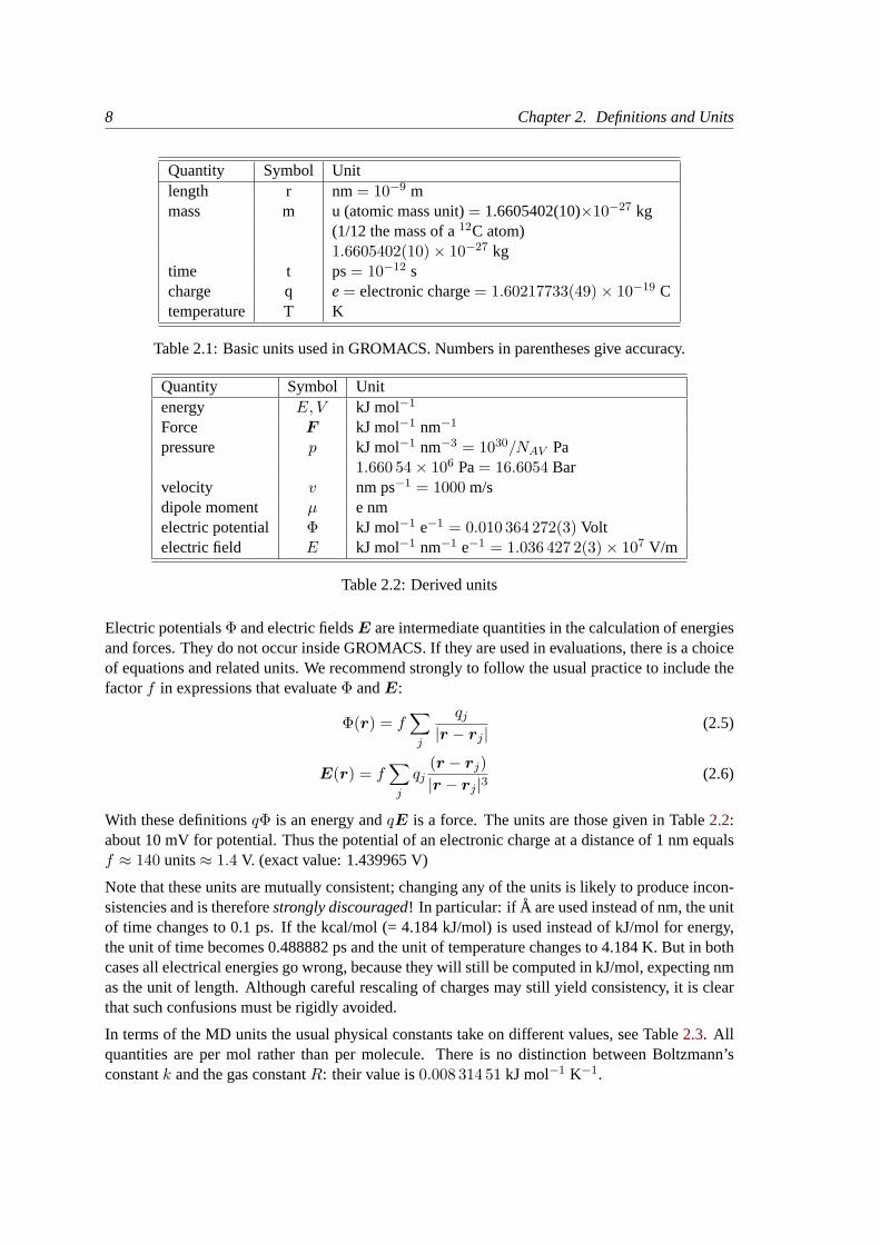
8 Chapter 2. Definitions and Units
Quantity Symbol Unitlength r nm= 10−9 mmass m u (atomic mass unit)= 1.6605402(10)×10−27 kg
(1/12 the mass of a12C atom)1.6605402(10)× 10−27 kg
time t ps= 10−12 scharge q e= electronic charge= 1.60217733(49)× 10−19 Ctemperature T K
Table 2.1: Basic units used in GROMACS. Numbers in parentheses give accuracy.
Quantity Symbol Unitenergy E, V kJ mol−1
Force F kJ mol−1 nm−1
pressure p kJ mol−1 nm−3 = 1030/NAV Pa1.660 54× 106 Pa= 16.6054 Bar
velocity v nm ps−1 = 1000 m/sdipole moment µ e nmelectric potential Φ kJ mol−1 e−1 = 0.010 364 272(3) Voltelectric field E kJ mol−1 nm−1 e−1 = 1.036 427 2(3)× 107 V/m
Table 2.2: Derived units
Electric potentialsΦ and electric fieldsE are intermediate quantities in the calculation of energiesand forces. They do not occur inside GROMACS. If they are used in evaluations, there is a choiceof equations and related units. We recommend strongly to follow the usual practice to include thefactorf in expressions that evaluateΦ andE:
Φ(r) = f∑j
qj|r − rj |
(2.5)
E(r) = f∑j
qj(r − rj)|r − rj |3
(2.6)
With these definitionsqΦ is an energy andqE is a force. The units are those given in Table2.2:about 10 mV for potential. Thus the potential of an electronic charge at a distance of 1 nm equalsf ≈ 140 units≈ 1.4 V. (exact value: 1.439965 V)
Note that these units are mutually consistent; changing any of the units is likely to produce incon-sistencies and is thereforestrongly discouraged! In particular: if A are used instead of nm, the unitof time changes to 0.1 ps. If the kcal/mol (= 4.184 kJ/mol) is used instead of kJ/mol for energy,the unit of time becomes 0.488882 ps and the unit of temperature changes to 4.184 K. But in bothcases all electrical energies go wrong, because they will still be computed in kJ/mol, expecting nmas the unit of length. Although careful rescaling of charges may still yield consistency, it is clearthat such confusions must be rigidly avoided.
In terms of the MD units the usual physical constants take on different values, see Table2.3. Allquantities are per mol rather than per molecule. There is no distinction between Boltzmann’sconstantk and the gas constantR: their value is0.008 314 51 kJ mol−1 K−1.
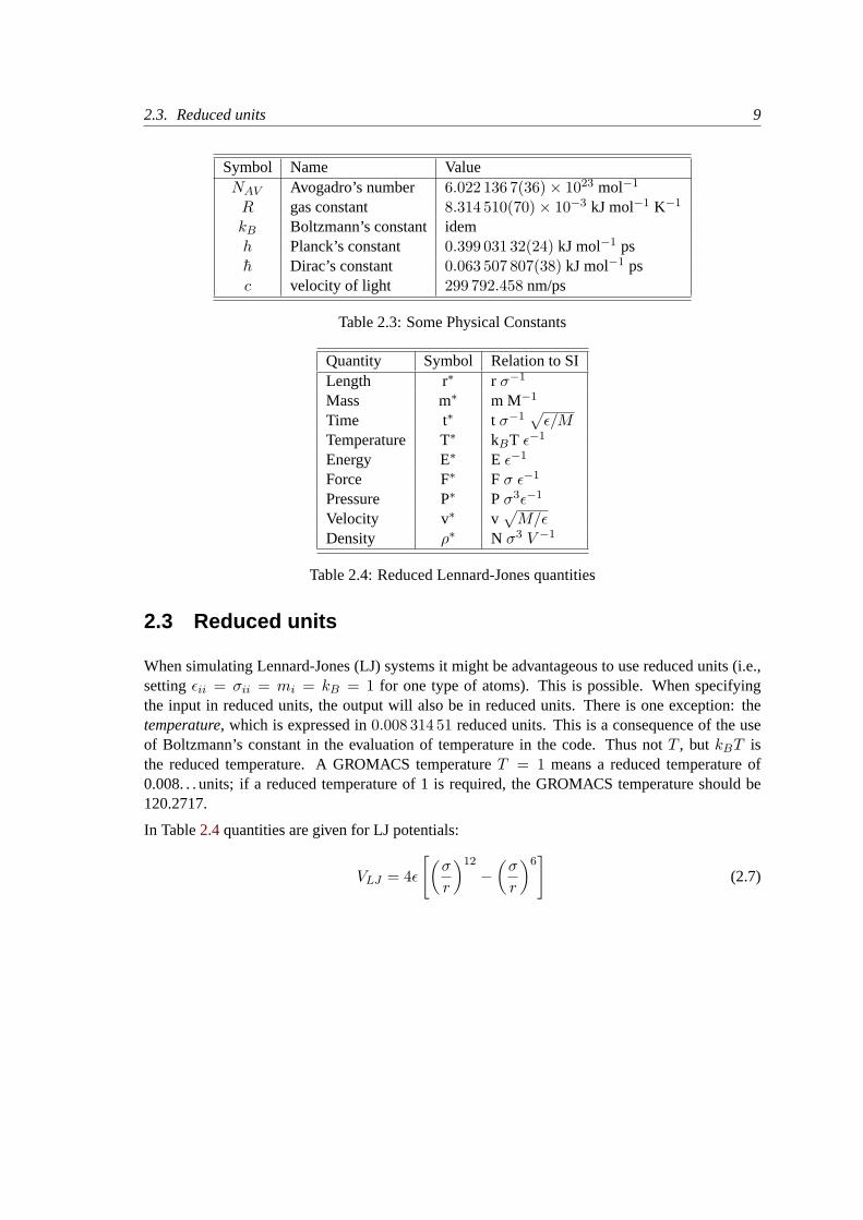
2.3. Reduced units 9
Symbol Name ValueNAV Avogadro’s number 6.022 136 7(36)× 1023 mol−1
R gas constant 8.314 510(70)× 10−3 kJ mol−1 K−1
kB Boltzmann’s constant idemh Planck’s constant 0.399 031 32(24) kJ mol−1 psh Dirac’s constant 0.063 507 807(38) kJ mol−1 psc velocity of light 299 792.458 nm/ps
Table 2.3: Some Physical Constants
Quantity Symbol Relation to SILength r∗ r σ−1
Mass m∗ m M−1
Time t∗ t σ−1√ε/M
Temperature T∗ kBT ε−1
Energy E∗ E ε−1
Force F∗ F σ ε−1
Pressure P∗ Pσ3ε−1
Velocity v∗ v√M/ε
Density ρ∗ N σ3 V −1
Table 2.4: Reduced Lennard-Jones quantities
2.3 Reduced units
When simulating Lennard-Jones (LJ) systems it might be advantageous to use reduced units (i.e.,settingεii = σii = mi = kB = 1 for one type of atoms). This is possible. When specifyingthe input in reduced units, the output will also be in reduced units. There is one exception: thetemperature, which is expressed in0.008 314 51 reduced units. This is a consequence of the useof Boltzmann’s constant in the evaluation of temperature in the code. Thus notT , but kBT isthe reduced temperature. A GROMACS temperatureT = 1 means a reduced temperature of0.008. . . units; if a reduced temperature of 1 is required, the GROMACS temperature should be120.2717.
In Table2.4quantities are given for LJ potentials:
VLJ = 4ε
[(σ
r
)12
−(σ
r
)6]
(2.7)

10 Chapter 2. Definitions and Units

Chapter 3
Algorithms
3.1 Introduction
In this chapter we first give describe two general concepts used in GROMACS:periodic boundaryconditions(sec.3.2) and thegroup concept(sec.3.3). The MD algorithm is described in sec.3.4:first a global form of the algorithm is given, which is refined in subsequent subsections. The(simple) EM (Energy Minimization) algorithm is described in sec.3.10. Some other algorithmsfor special purpose dynamics are described after this. In the final sec.3.14of this chapter a fewprinciples are given on which parallelization of GROMACS is based. The parallelization is hardlyvisible for the user and is therefore not treated in detail.
A few issues are of general interest. In all cases thesystemmust be defined, consisting ofmolecules. Molecules again consist of particles with defined interaction functions. The detaileddescription of thetopologyof the molecules and of theforce fieldand the calculation of forces isgiven in chapter4. In the present chapter we describe other aspects of the algorithm, such as pairlist generation, update of velocities and positions, coupling to external temperature and pressure,conservation of constraints. Theanalysisof the data generated by an MD simulation is treated inchapter8.
3.2 Periodic boundary conditions
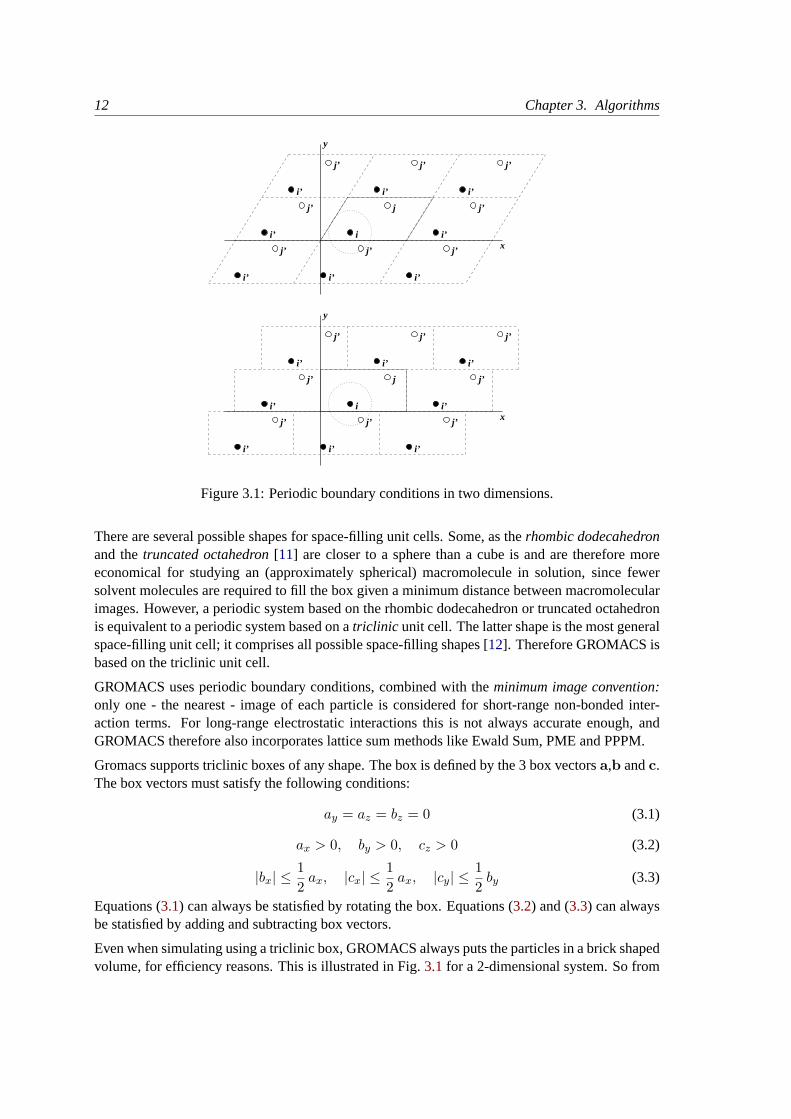
The classical way to minimize edge effects in a finite system is to applyperiodic boundary condi-tions. The atoms of the system to be simulated are put into a space-filling box, which is surroundedby translated copies of itself (Fig.3.1). Thus there are no boundaries of the system; the artifactcaused by unwanted boundaries in an isolated cluster is now replaced by the artifact of periodicconditions. If a crystal is simulated, such boundary conditions are desired (although motions arenaturally restricted to periodic motions with wavelengths fitting into the box). If one wishes tosimulate non-periodic systems, as liquids or solutions, the periodicity by itself causes errors. Theerrors can be evaluated by comparing various system sizes; they are expected to be less severethan the errors resulting from an unnatural boundary with vacuum.
12 Chapter 3. Algorithms
j’ j’
i’ i’i’
i’
j’
i’ i’
y
x
y
x
j’ j’
i’
i’
i’i
j’
j’ j’j’
i’ii’
j’j’
j’
j
i’ i’i’
j’
i’ i’
j’
j’j’
j
Figure 3.1: Periodic boundary conditions in two dimensions.
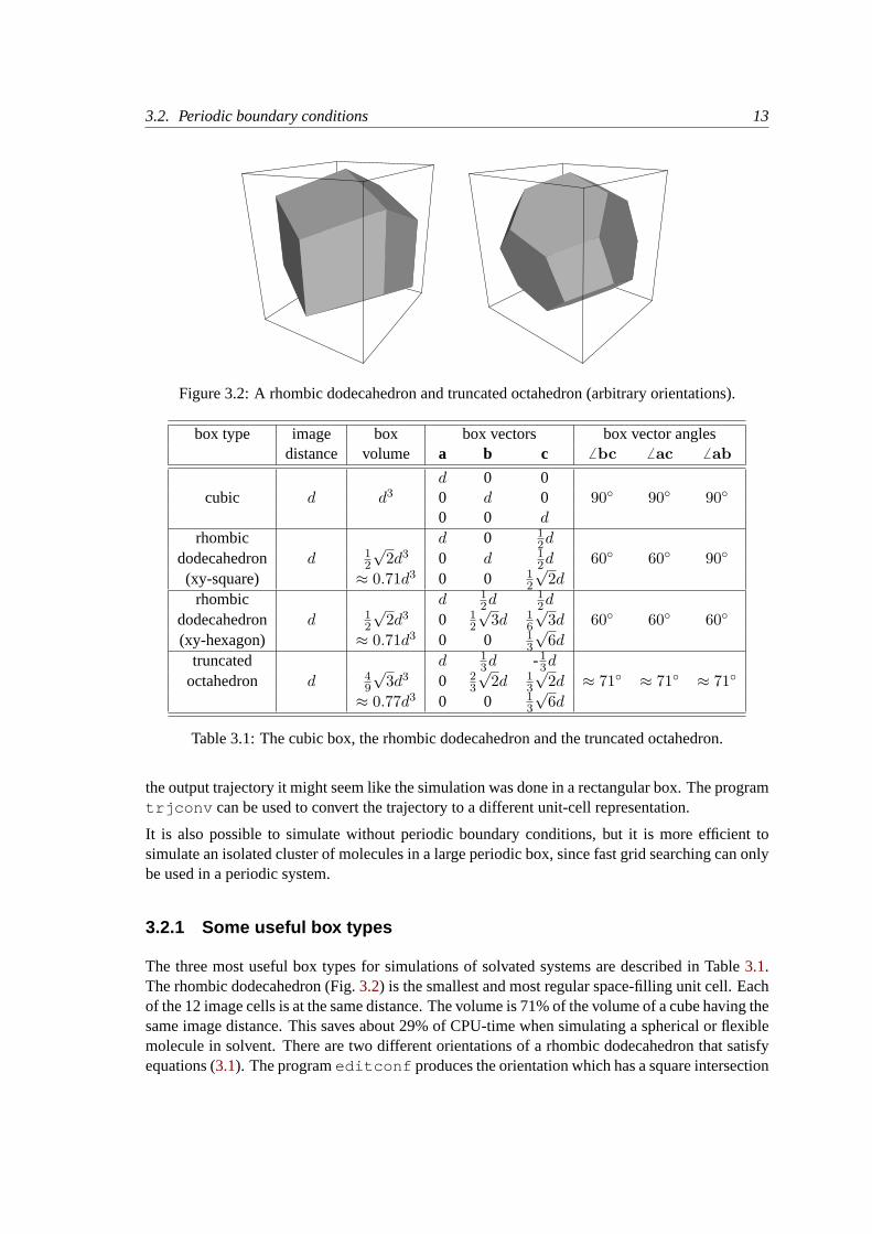
There are several possible shapes for space-filling unit cells. Some, as therhombic dodecahedronand thetruncated octahedron[11] are closer to a sphere than a cube is and are therefore moreeconomical for studying an (approximately spherical) macromolecule in solution, since fewersolvent molecules are required to fill the box given a minimum distance between macromolecularimages. However, a periodic system based on the rhombic dodecahedron or truncated octahedronis equivalent to a periodic system based on atriclinic unit cell. The latter shape is the most generalspace-filling unit cell; it comprises all possible space-filling shapes [12]. Therefore GROMACS isbased on the triclinic unit cell.
GROMACS uses periodic boundary conditions, combined with theminimum image convention:only one - the nearest - image of each particle is considered for short-range non-bonded inter-action terms. For long-range electrostatic interactions this is not always accurate enough, andGROMACS therefore also incorporates lattice sum methods like Ewald Sum, PME and PPPM.
Gromacs supports triclinic boxes of any shape. The box is defined by the 3 box vectorsa,b andc.The box vectors must satisfy the following conditions:
ay = az = bz = 0 (3.1)
ax > 0, by > 0, cz > 0 (3.2)
|bx| ≤12ax, |cx| ≤
12ax, |cy| ≤
12by (3.3)
Equations (3.1) can always be statisfied by rotating the box. Equations (3.2) and (3.3) can alwaysbe statisfied by adding and subtracting box vectors.
Even when simulating using a triclinic box, GROMACS always puts the particles in a brick shapedvolume, for efficiency reasons. This is illustrated in Fig.3.1 for a 2-dimensional system. So from
3.2. Periodic boundary conditions 13
Figure 3.2: A rhombic dodecahedron and truncated octahedron (arbitrary orientations).
box type image box box vectors box vector anglesdistance volume a b c 6 bc 6 ac 6 ab
d 0 0cubic d d3 0 d 0 90◦ 90◦ 90◦
0 0 d
rhombic d 0 12d
dodecahedron d 12
√2d3 0 d 1
2d 60◦ 60◦ 90◦
(xy-square) ≈ 0.71d3 0 0 12
√2d
rhombic d 12d
12d
dodecahedron d 12
√2d3 0 1
2
√3d 1
6
√3d 60◦ 60◦ 60◦
(xy-hexagon) ≈ 0.71d3 0 0 13
√6d
truncated d 13d -1
3d
octahedron d 49
√3d3 0 2
3
√2d 1
3
√2d ≈ 71◦ ≈ 71◦ ≈ 71◦
≈ 0.77d3 0 0 13
√6d
Table 3.1: The cubic box, the rhombic dodecahedron and the truncated octahedron.
the output trajectory it might seem like the simulation was done in a rectangular box. The programtrjconv can be used to convert the trajectory to a different unit-cell representation.
It is also possible to simulate without periodic boundary conditions, but it is more efficient tosimulate an isolated cluster of molecules in a large periodic box, since fast grid searching can onlybe used in a periodic system.
3.2.1 Some useful box types
The three most useful box types for simulations of solvated systems are described in Table3.1.The rhombic dodecahedron (Fig.3.2) is the smallest and most regular space-filling unit cell. Eachof the 12 image cells is at the same distance. The volume is 71% of the volume of a cube having thesame image distance. This saves about 29% of CPU-time when simulating a spherical or flexiblemolecule in solvent. There are two different orientations of a rhombic dodecahedron that satisfyequations (3.1). The programeditconf produces the orientation which has a square intersection
14 Chapter 3. Algorithms
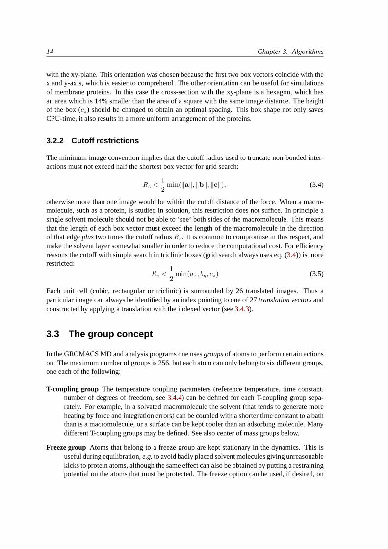
with the xy-plane. This orientation was chosen because the first two box vectors coincide with thex and y-axis, which is easier to comprehend. The other orientation can be useful for simulationsof membrane proteins. In this case the cross-section with the xy-plane is a hexagon, which hasan area which is 14% smaller than the area of a square with the same image distance. The heightof the box (cz) should be changed to obtain an optimal spacing. This box shape not only savesCPU-time, it also results in a more uniform arrangement of the proteins.
3.2.2 Cutoff restrictions
The minimum image convention implies that the cutoff radius used to truncate non-bonded inter-actions must not exceed half the shortest box vector for grid search:
Rc <12
min(‖a‖, ‖b‖, ‖c‖), (3.4)
otherwise more than one image would be within the cutoff distance of the force. When a macro-molecule, such as a protein, is studied in solution, this restriction does not suffice. In principle asingle solvent molecule should not be able to ‘see’ both sides of the macromolecule. This meansthat the length of each box vector must exceed the length of the macromolecule in the directionof that edgeplus two times the cutoff radiusRc. It is common to compromise in this respect, andmake the solvent layer somewhat smaller in order to reduce the computational cost. For efficiencyreasons the cutoff with simple search in triclinic boxes (grid search always uses eq. (3.4)) is morerestricted:
Rc <12
min(ax, by, cz) (3.5)
Each unit cell (cubic, rectangular or triclinic) is surrounded by 26 translated images. Thus aparticular image can always be identified by an index pointing to one of 27translation vectorsandconstructed by applying a translation with the indexed vector (see3.4.3).
3.3 The group concept
In the GROMACS MD and analysis programs one usesgroupsof atoms to perform certain actionson. The maximum number of groups is 256, but each atom can only belong to six different groups,one each of the following:
T-coupling group The temperature coupling parameters (reference temperature, time constant,number of degrees of freedom, see3.4.4) can be defined for each T-coupling group sepa-rately. For example, in a solvated macromolecule the solvent (that tends to generate moreheating by force and integration errors) can be coupled with a shorter time constant to a baththan is a macromolecule, or a surface can be kept cooler than an adsorbing molecule. Manydifferent T-coupling groups may be defined. See also center of mass groups below.
Freeze group Atoms that belong to a freeze group are kept stationary in the dynamics. This isuseful during equilibration,e.g.to avoid badly placed solvent molecules giving unreasonablekicks to protein atoms, although the same effect can also be obtained by putting a restrainingpotential on the atoms that must be protected. The freeze option can be used, if desired, on
3.4. Molecular Dynamics 15
just one or two coordinates of an atom, thereby freezing the atoms in a plane or on a line.Many freeze groups can be defined.
Accelerate group On each atom in an ’accelerate group’ an accelerationag is imposed. Thisis equivalent to an external force. This feature makes it possible to drive the system intoa non-equilibrium state and enables the performance of non-equilibrium MD and hence toobtain transport properties.
Energy monitor group Mutual interactions between all energy monitor groups are compiled dur-ing the simulation. This is done separately for Lennard-Jones and Coulomb terms. In prin-ciple up to 256 groups could be defined, but that would lead to 256×256 items! Better usethis concept sparingly.
All non-bonded interactions between pairs of energy monitor groups can be excluded (seesec.7.3.1). Pairs of particles from excluded pairs of energy monitor groups are not putinto the pair list. This can result in a significant speedup for simulations where interactionswithin or between parts of the system are not required.
Center of mass group In GROMACS the center of mass (COM) motion can be removed, foreither the complete system or for groups of atoms. The latter is useful,e.g. for systemswhere there is limited friction (e.g.gas systems) to prevent center of mass motion to occur.It makes sense to use the same groups for Temperature coupling and center of mass motionremoval.
XTC output group In order to reduce the size of the XTC trajectory file, only a subset of allparticles can be stored. All XTC groups that are specified are saved, the rest is not. If noXTC groups are specified, than all atoms are saved to the XTC file.
The use of groups in analysis programs is described in chapter8.
3.4 Molecular Dynamics
A global flow scheme for MD is given in Fig.3.3. Each MD or EM run requires as input a set ofinitial coordinates and - optionally - initial velocities of all particles involved. This chapter doesnot describe how these are obtained; for the setup of an actual MD run check the online manual atwww.gromacs.org.
3.4.1 Initial conditions
Topology and force field
The system topology, including a description of the force field, must be loaded. These items aredescribed in chapter4. All this information is static; it is never modified during the run.

16 Chapter 3. Algorithms
THE GLOBAL MD ALGORITHM
1. Input initial conditions
Potential interactionV as a function of atom positionsPositionsr of all atoms in the systemVelocitiesv of all atoms in the system
⇓
repeat 2,3,4for the required number of steps:
2. Compute forces
The force on any atom
F i = − ∂V∂ri
is computed by calculating the force between non-bonded atompairs:
F i =∑
j F ij
plus the forces due to bonded interactions (which may depend on 1,2, 3, or 4 atoms), plus restraining and/or external forces.
The potential and kinetic energies and the pressure tensor arecomputed.
⇓3. Update configuration
The movement of the atoms is simulated by numerically solvingNewton’s equations of motion
d2ri
dt2=
F i
miordri
dt= vi;
dvi
dt=
F i
mi
⇓4. if required:Output step
write positions, velocities, energies, temperature, pressure, etc.
Figure 3.3: The global MD algorithm
3.4. Molecular Dynamics 17
0�
Velocity�
0.0
Pro
babi
lity
�
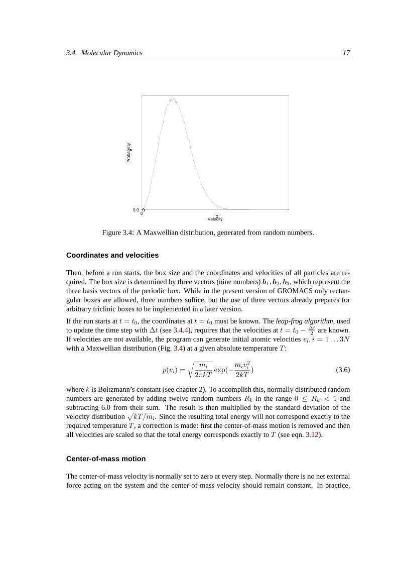
Figure 3.4: A Maxwellian distribution, generated from random numbers.
Coordinates and velocities
Then, before a run starts, the box size and the coordinates and velocities of all particles are re-quired. The box size is determined by three vectors (nine numbers)b1, b2, b3, which represent thethree basis vectors of the periodic box. While in the present version of GROMACS only rectan-gular boxes are allowed, three numbers suffice, but the use of three vectors already prepares forarbitrary triclinic boxes to be implemented in a later version.
If the run starts att = t0, the coordinates att = t0 must be known. Theleap-frog algorithm,usedto update the time step with∆t (see3.4.4), requires that the velocities att = t0 − ∆t
2 are known.If velocities are not available, the program can generate initial atomic velocitiesvi, i = 1 . . . 3Nwith a Maxwellian distribution (Fig.3.4) at a given absolute temperatureT :
p(vi) =√
mi
2πkTexp(−miv
2i
2kT) (3.6)
wherek is Boltzmann’s constant (see chapter2). To accomplish this, normally distributed randomnumbers are generated by adding twelve random numbersRk in the range0 ≤ Rk < 1 andsubtracting 6.0 from their sum. The result is then multiplied by the standard deviation of thevelocity distribution
√kT/mi. Since the resulting total energy will not correspond exactly to the
required temperatureT , a correction is made: first the center-of-mass motion is removed and thenall velocities are scaled so that the total energy corresponds exactly toT (see eqn.3.12).
Center-of-mass motion
The center-of-mass velocity is normally set to zero at every step. Normally there is no net externalforce acting on the system and the center-of-mass velocity should remain constant. In practice,
18 Chapter 3. Algorithms
however, the update algorithm develops a very slow change in the center-of-mass velocity, andthus in the total kinetic energy of the system, specially when temperature coupling is used. If suchchanges are not quenched, an appreciable center-of-mass motion develops eventually in long runs,and the temperature will be significantly misinterpreted. The same may happen due to overallrotational motion, but only when an isolated cluster is simulated. In periodic systems with filledboxes, the overall rotational motion is coupled to other degrees of freedom and does not give anyproblems.
3.4.2 Neighbor searching
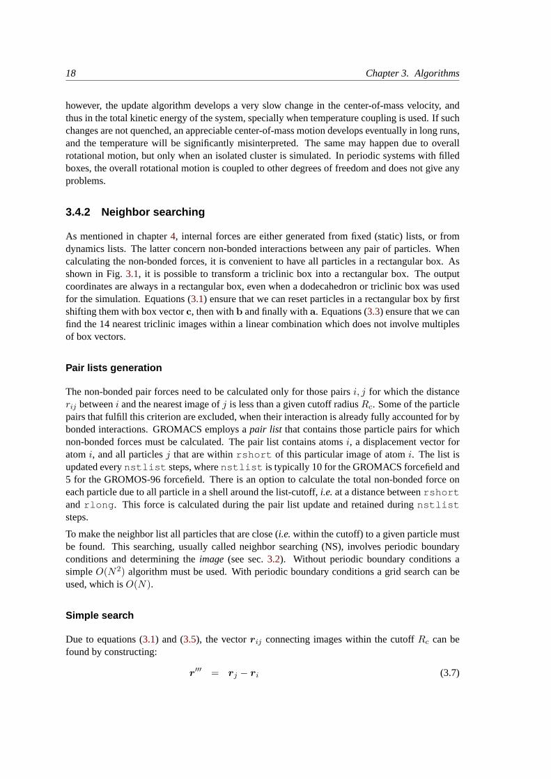
As mentioned in chapter4, internal forces are either generated from fixed (static) lists, or fromdynamics lists. The latter concern non-bonded interactions between any pair of particles. Whencalculating the non-bonded forces, it is convenient to have all particles in a rectangular box. Asshown in Fig.3.1, it is possible to transform a triclinic box into a rectangular box. The outputcoordinates are always in a rectangular box, even when a dodecahedron or triclinic box was usedfor the simulation. Equations (3.1) ensure that we can reset particles in a rectangular box by firstshifting them with box vectorc, then withb and finally witha. Equations (3.3) ensure that we canfind the 14 nearest triclinic images within a linear combination which does not involve multiplesof box vectors.
Pair lists generation
The non-bonded pair forces need to be calculated only for those pairsi, j for which the distancerij betweeni and the nearest image ofj is less than a given cutoff radiusRc. Some of the particlepairs that fulfill this criterion are excluded, when their interaction is already fully accounted for bybonded interactions. GROMACS employs apair list that contains those particle pairs for whichnon-bonded forces must be calculated. The pair list contains atomsi, a displacement vector foratomi, and all particlesj that are withinrshort of this particular image of atomi. The list isupdated everynstlist steps, wherenstlist is typically 10 for the GROMACS forcefield and5 for the GROMOS-96 forcefield. There is an option to calculate the total non-bonded force oneach particle due to all particle in a shell around the list-cutoff,i.e.at a distance betweenrshortand rlong . This force is calculated during the pair list update and retained duringnstliststeps.
To make the neighbor list all particles that are close (i.e.within the cutoff) to a given particle mustbe found. This searching, usually called neighbor searching (NS), involves periodic boundaryconditions and determining theimage (see sec.3.2). Without periodic boundary conditions asimpleO(N2) algorithm must be used. With periodic boundary conditions a grid search can beused, which isO(N).
Simple search
Due to equations (3.1) and (3.5), the vectorrij connecting images within the cutoffRc can befound by constructing:
r′′′ = rj − ri (3.7)
3.4. Molecular Dynamics 19
� � � � �� � � � �
� � � �� � � �
� � � � � � � � �� � � � � � � � �� � � � � � � � �
� � � � � � � �� � � � � � � �� � � � � � � �
� � � � � � � � � �� � � � � � � � � �� � � � � � � � � �� � � � � � � � � �� � � � � � � � � �
� � � � � � � � � �� � � � � � � � � �� � � � � � � � � �� � � � � � � � � �� � � � � � � � � �� � � � � � �
� � � � � � �� � � � � �� � � � � �
� � �� � � j
i
i’
� � � � � � � � � � � � � � �� � � � �� � � � �� � � � �� � � � �� � � � �� � � � �� � � � �� � � � �
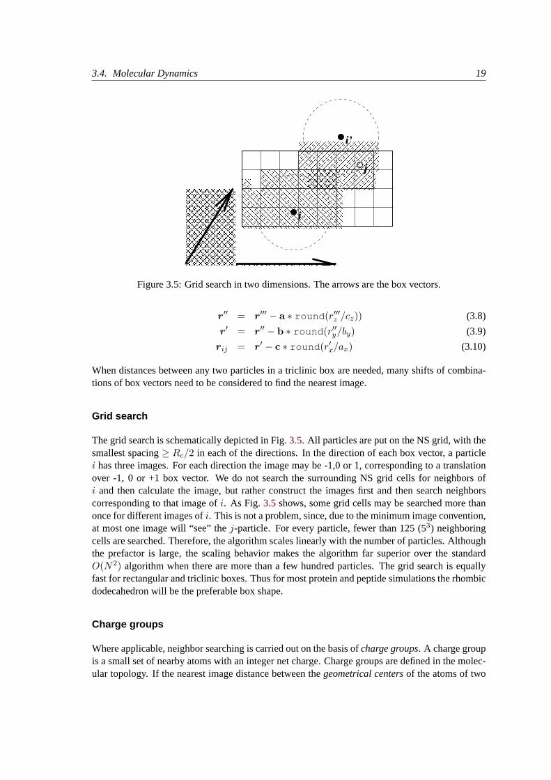
Figure 3.5: Grid search in two dimensions. The arrows are the box vectors.
r′′ = r′′′ − a ∗ round (r′′′z /cz)) (3.8)
r′ = r′′ − b ∗ round (r′′y/by) (3.9)
rij = r′ − c ∗ round (r′x/ax) (3.10)
When distances between any two particles in a triclinic box are needed, many shifts of combina-tions of box vectors need to be considered to find the nearest image.
Grid search
The grid search is schematically depicted in Fig.3.5. All particles are put on the NS grid, with thesmallest spacing≥ Rc/2 in each of the directions. In the direction of each box vector, a particlei has three images. For each direction the image may be -1,0 or 1, corresponding to a translationover -1, 0 or +1 box vector. We do not search the surrounding NS grid cells for neighbors ofi and then calculate the image, but rather construct the images first and then search neighborscorresponding to that image ofi. As Fig.3.5 shows, some grid cells may be searched more thanonce for different images ofi. This is not a problem, since, due to the minimum image convention,at most one image will “see” thej-particle. For every particle, fewer than 125 (53) neighboringcells are searched. Therefore, the algorithm scales linearly with the number of particles. Althoughthe prefactor is large, the scaling behavior makes the algorithm far superior over the standardO(N2) algorithm when there are more than a few hundred particles. The grid search is equallyfast for rectangular and triclinic boxes. Thus for most protein and peptide simulations the rhombicdodecahedron will be the preferable box shape.
Charge groups
Where applicable, neighbor searching is carried out on the basis ofcharge groups. A charge groupis a small set of nearby atoms with an integer net charge. Charge groups are defined in the molec-ular topology. If the nearest image distance between thegeometrical centersof the atoms of two
20 Chapter 3. Algorithms
charge groups is less than the cutoff radius, all atom pairs between the charge groups are includedin the pair list. This procedure avoids the creation of charges due to the use of a cutoff (when onecharge of a dipole is within range and the other not), which can have disastrous consequences forthe behavior of the Coulomb interaction function at distances near the cutoff radius. If moleculargroups have full charges (ions), charge groups do not avoid adverse cutoff effects, and you shouldconsider using one of the lattice sum methods supplied by GROMACS [13].
If appropriately constructed shift functions are used for the electrostatic forces, no charge groupsare needed. Such shift functions are implemented in GROMACS (see chapter4) but must be usedwith care: in principle, they should be combined with a lattice sum for long-range electrostatics.
3.4.3 Compute forces
Potential energy
When forces are computed, the potential energy of each interaction term is computed as well.The total potential energy is summed for various contributions, such as Lennard-Jones, Coulomb,and bonded terms. It is also possible to compute these contributions forgroupsof atoms that areseparately defined (see sec.3.3).
Kinetic energy and temperature
The temperature is given by the total kinetic energy of theN -particle system:
Ekin =12
N∑i=1
miv2i (3.11)
From this the absolute temperatureT can be computed using:
12NdfkT = Ekin (3.12)
wherek is Boltzmann’s constant andNdf is the number of degrees of freedom which can becomputed from:
Ndf = 3N −Nc −Ncom (3.13)
HereNc is the number ofconstraintsimposed on the system. When performing molecular dynam-icsNcom = 3 additional degrees of freedom must be removed, because the three center-of-massvelocities are constants of the motion, which are usually set to zero. When simulating in vacuo,the rotation around the center of mass can also be removed, in this caseNcom = 6. When morethan one temperature coupling group is used, the number of degrees of freedom for groupi is:
N idf = (3N i −N i
c)3N −Nc −Ncom
3N −Nc(3.14)
The kinetic energy can also be written as a tensor, which is necessary for pressure calculation in atriclinic system, or systems where shear forces are imposed:
Ekin =12
N∑i
mivi ⊗ vi (3.15)
3.4. Molecular Dynamics 21
1 20 t
x v x
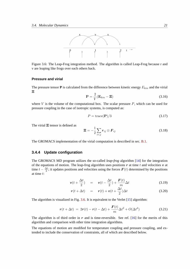
Figure 3.6: The Leap-Frog integration method. The algorithm is called Leap-Frog because r andv are leaping like frogs over each others back.
Pressure and virial
The pressure tensorP is calculated from the difference between kinetic energyEkin and the virialΞ
P =2V
(Ekin −Ξ) (3.16)
whereV is the volume of the computational box. The scalar pressureP , which can be used forpressure coupling in the case of isotropic systems, is computed as:
P = trace(P)/3 (3.17)
The virialΞ tensor is defined as
Ξ = −12
∑i<j
rij ⊗ F ij (3.18)
The GROMACS implementation of the virial computation is described in sec.B.1.
3.4.4 Update configuration
The GROMACS MD program utilizes the so-calledleap-frogalgorithm [14] for the integrationof the equations of motion. The leap-frog algorithm uses positionsr at timet and velocitiesv attime t− ∆t
2 ; it updates positions and velocities using the forcesF (t) determined by the positionsat timet:
v(t+∆t2
) = v(t− ∆t2
) +F (t)m
∆t (3.19)
r(t+ ∆t) = r(t) + v(t+∆t2
)∆t (3.20)
The algorithm is visualized in Fig.3.6. It is equivalent to the Verlet [15] algorithm:
r(t+ ∆t) = 2r(t)− r(t−∆t) +F (t)m
∆t2 +O(∆t4) (3.21)
The algorithm is of third order inr and is time-reversible. See ref. [16] for the merits of thisalgorithm and comparison with other time integration algorithms.
The equations of motion are modified for temperature coupling and pressure coupling, and ex-tended to include the conservation of constraints, all of which are described below.
22 Chapter 3. Algorithms
3.4.5 Temperature coupling
For several reasons (drift during equilibration, drift as a result of force truncation and integrationerrors, heating due to external or frictional forces), it is necessary to control the temperature of thesystem. GROMACS can use either theweak couplingscheme of Berendsen [17] or the extendedensemble Nose-Hoover scheme [18, 19].
Berendsen temperature coupling
The Berendsen algorithm mimics weak coupling with first-order kinetics to an external heat bathwith given temperatureT0. See ref. [20] for a comparison with the Nose-Hoover scheme. Theeffect of this algorithm is that a deviation of the system temperature fromT0 is slowly correctedaccording to
dTdt
=T0 − T
τ(3.22)
which means that a temperature deviation decays exponentially with a time constantτ . Thismethod of coupling has the advantage that the strength of the coupling can be varied and adaptedto the user requirement: for equilibration purposes the coupling time can be taken quite short (e.g.0.01 ps), but for reliable equilibrium runs it can be taken much longer (e.g.0.5 ps) in which caseit hardly influences the conservative dynamics.
The heat flow into or out of the system is effected by scaling the velocities of each particle everystep with a time-dependent factorλ, given by
λ =
[1 +
∆tτT
{T0
T (t− ∆t2 )
− 1
}]1/2
(3.23)
The parameterτT is close to, but not exactly equal to the time constantτ of the temperaturecoupling (eqn.3.22):
τ = 2CV τT /Ndfk (3.24)
whereCV is the total heat capacity of the system,k is Boltzmann’s constant, andNdf is thetotal number of degrees of freedom. The reason thatτ 6= τT is that the kinetic energy changecaused by scaling the velocities is partly redistributed between kinetic and potential energy andhence the change in temperature is less than the scaling energy. In practice, the ratioτ/τT rangesfrom 1 (gas) to 2 (harmonic solid) to 3 (water). When we use the term ’temperature couplingtime constant’, we mean the parameterτT . Note that in practice the scaling factorλ is limitedto the range of 0.8<= λ <= 1.25, to avoid scaling by very large numbers which may crash thesimulation. In normal use,λ will always be much closer to 1.0.
Strictly, for computing the scaling factor the temperatureT is needed at timet, but this is notavailable in the algorithm. In practice, the temperature at the previous time step is used (as indi-cated in eqn.3.23), which is perfectly all right since the coupling time constant is much longerthan one time step. The Berendsen algorithm is stable up toτT ≈ ∆t. [A simple steepest-descentminimizer can be implemented by settingT = 0 andτT � δt.]
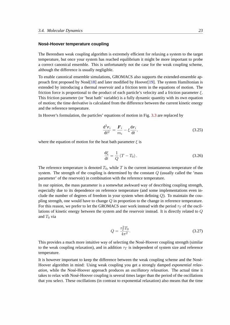
3.4. Molecular Dynamics 23
Nose-Hoover temperature coupling
The Berendsen weak coupling algorithm is extremely efficient for relaxing a system to the targettemperature, but once your system has reached equilibrium it might be more important to probea correct canonical ensemble. This is unfortunately not the case for the weak coupling scheme,although the difference is usually negligible.
To enable canonical ensemble simulations, GROMACS also supports the extended-ensemble ap-proach first proposed by Nose[18] and later modified by Hoover[19]. The system Hamiltonian isextended by introducing a thermal reservoir and a friction term in the equations of motion. Thefriction force is proportional to the product of each particle’s velocity and a friction parameterξ.This friction parameter (or ’heat bath’ variable) is a fully dynamic quantity with its own equationof motion; the time derivative is calculated from the difference between the current kinetic energyand the reference temperature.
In Hoover’s formulation, the particles’ equations of motion in Fig.3.3are replaced by
d2ri
dt2=
F i
mi− ξ
dri
dt, (3.25)
where the equation of motion for the heat bath parameterξ is
dξdt
=1Q
(T − T0) . (3.26)
The reference temperature is denotedT0, while T is the current instantaneous temperature of thesystem. The strength of the coupling is determined by the constantQ (usually called the ’massparameter’ of the reservoir) in combination with the reference temperature.
In our opinion, the mass parameter is a somewhat awkward way of describing coupling strength,especially due to its dependence on reference temperature (and some implementations even in-clude the number of degrees of freedom in your system when definingQ). To maintain the cou-pling strength, one would have to changeQ in proportion to the change in reference temperature.For this reason, we prefer to let the GROMACS user work instead with the periodτT of the oscil-lations of kinetic energy between the system and the reservoir instead. It is directly related toQandT0 via
Q =τ2TT0
4π2. (3.27)
This provides a much more intuitive way of selecting the Nose-Hoover coupling strength (similarto the weak coupling relaxation), and in additionτT is independent of system size and referencetemperature.
It is however important to keep the difference between the weak coupling scheme and the Nose-Hoover algorithm in mind: Using weak coupling you get a strongly dampedexponential relax-ation, while the Nose-Hoover approach produces anoscillatory relaxation. The actual time ittakes to relax with Nose-Hoover coupling is several times larger than the period of the oscillationsthat you select. These oscillations (in contrast to exponential relaxation) also means that the time
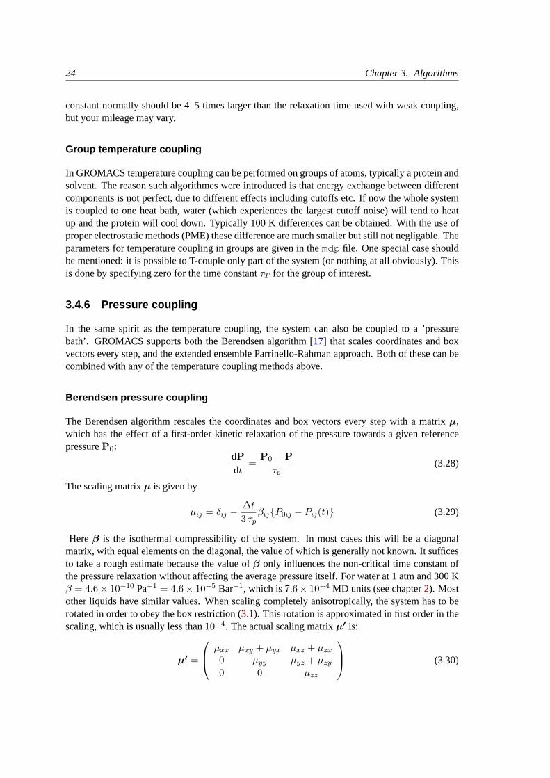
24 Chapter 3. Algorithms
constant normally should be 4–5 times larger than the relaxation time used with weak coupling,but your mileage may vary.
Group temperature coupling
In GROMACS temperature coupling can be performed on groups of atoms, typically a protein andsolvent. The reason such algorithmes were introduced is that energy exchange between differentcomponents is not perfect, due to different effects including cutoffs etc. If now the whole systemis coupled to one heat bath, water (which experiences the largest cutoff noise) will tend to heatup and the protein will cool down. Typically 100 K differences can be obtained. With the use ofproper electrostatic methods (PME) these difference are much smaller but still not negligable. Theparameters for temperature coupling in groups are given in themdpfile. One special case shouldbe mentioned: it is possible to T-couple only part of the system (or nothing at all obviously). Thisis done by specifying zero for the time constantτT for the group of interest.
3.4.6 Pressure coupling
In the same spirit as the temperature coupling, the system can also be coupled to a ’pressurebath’. GROMACS supports both the Berendsen algorithm [17] that scales coordinates and boxvectors every step, and the extended ensemble Parrinello-Rahman approach. Both of these can becombined with any of the temperature coupling methods above.
Berendsen pressure coupling
The Berendsen algorithm rescales the coordinates and box vectors every step with a matrixµ,which has the effect of a first-order kinetic relaxation of the pressure towards a given referencepressureP0:
dPdt
=P0 −Pτp
(3.28)
The scaling matrixµ is given by
µij = δij −∆t3 τp
βij{P0ij − Pij(t)} (3.29)
Hereβ is the isothermal compressibility of the system. In most cases this will be a diagonalmatrix, with equal elements on the diagonal, the value of which is generally not known. It sufficesto take a rough estimate because the value ofβ only influences the non-critical time constant ofthe pressure relaxation without affecting the average pressure itself. For water at 1 atm and 300 Kβ = 4.6× 10⁻¹⁰ Pa−1 = 4.6× 10⁻⁵ Bar−1, which is7.6× 10−4 MD units (see chapter2). Mostother liquids have similar values. When scaling completely anisotropically, the system has to berotated in order to obey the box restriction (3.1). This rotation is approximated in first order in thescaling, which is usually less than10−4. The actual scaling matrixµ′ is:
µ′ =
µxx µxy + µyx µxz + µzx
0 µyy µyz + µzy
0 0 µzz
(3.30)
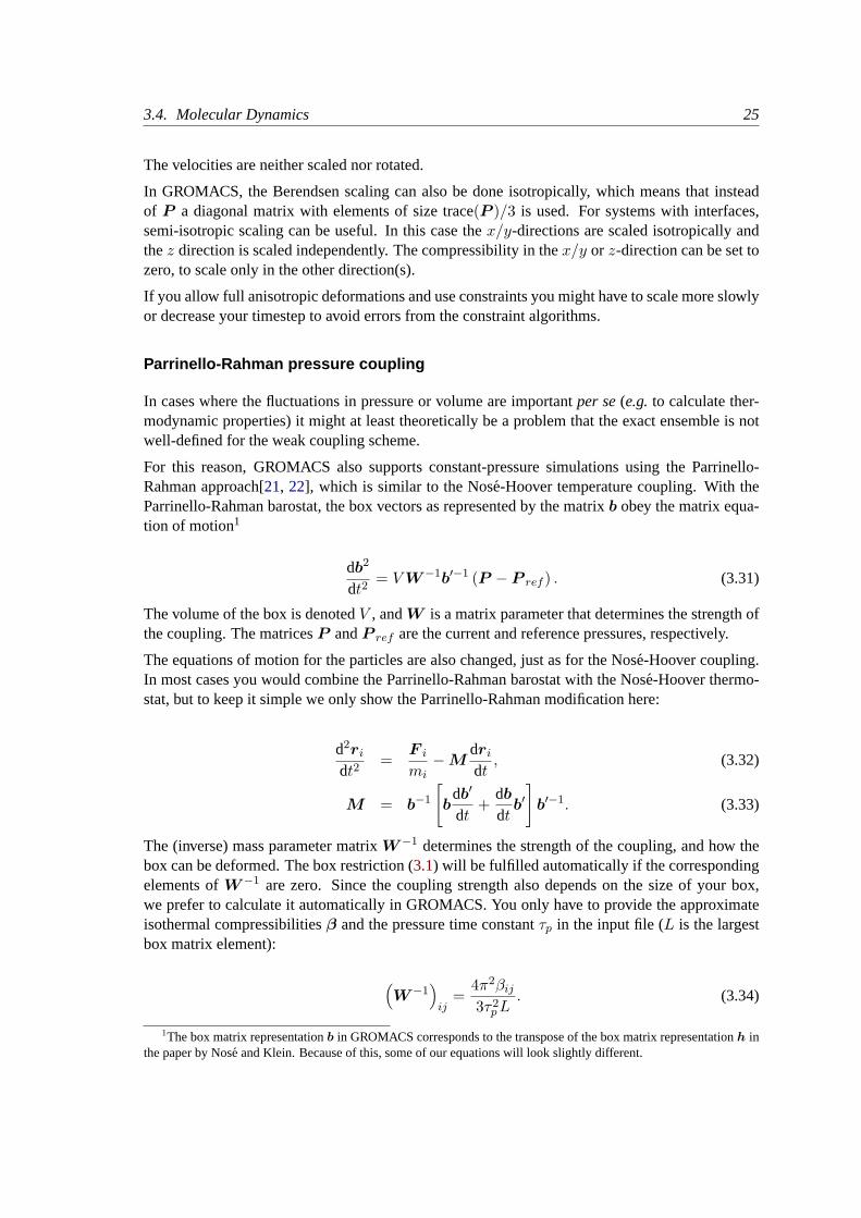
3.4. Molecular Dynamics 25
The velocities are neither scaled nor rotated.
In GROMACS, the Berendsen scaling can also be done isotropically, which means that insteadof P a diagonal matrix with elements of size trace(P )/3 is used. For systems with interfaces,semi-isotropic scaling can be useful. In this case thex/y-directions are scaled isotropically andthez direction is scaled independently. The compressibility in thex/y or z-direction can be set tozero, to scale only in the other direction(s).
If you allow full anisotropic deformations and use constraints you might have to scale more slowlyor decrease your timestep to avoid errors from the constraint algorithms.
Parrinello-Rahman pressure coupling
In cases where the fluctuations in pressure or volume are importantper se(e.g.to calculate ther-modynamic properties) it might at least theoretically be a problem that the exact ensemble is notwell-defined for the weak coupling scheme.
For this reason, GROMACS also supports constant-pressure simulations using the Parrinello-Rahman approach[21, 22], which is similar to the Nose-Hoover temperature coupling. With theParrinello-Rahman barostat, the box vectors as represented by the matrixb obey the matrix equa-tion of motion1
db2
dt2= VW−1b′−1 (P − P ref ) . (3.31)
The volume of the box is denotedV , andW is a matrix parameter that determines the strength ofthe coupling. The matricesP andP ref are the current and reference pressures, respectively.
The equations of motion for the particles are also changed, just as for the Nose-Hoover coupling.In most cases you would combine the Parrinello-Rahman barostat with the Nose-Hoover thermo-stat, but to keep it simple we only show the Parrinello-Rahman modification here:
d2ri
dt2=
F i
mi−M
dri
dt, (3.32)
M = b−1
[b
db′
dt+
db
dtb′]
b′−1. (3.33)
The (inverse) mass parameter matrixW−1 determines the strength of the coupling, and how thebox can be deformed. The box restriction (3.1) will be fulfilled automatically if the correspondingelements ofW−1 are zero. Since the coupling strength also depends on the size of your box,we prefer to calculate it automatically in GROMACS. You only have to provide the approximateisothermal compressibilitiesβ and the pressure time constantτp in the input file (L is the largestbox matrix element):
(W−1
)ij
=4π2βij
3τ2pL
. (3.34)
1The box matrix representationb in GROMACS corresponds to the transpose of the box matrix representationh inthe paper by Nose and Klein. Because of this, some of our equations will look slightly different.
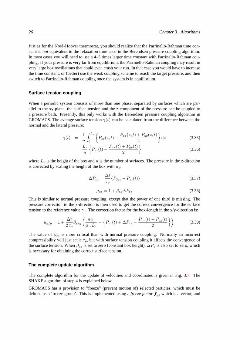
26 Chapter 3. Algorithms
Just as for the Nose-Hoover thermostat, you should realize that the Parrinello-Rahman time con-stant isnot equivalent to the relaxation time used in the Berendsen pressure coupling algorithm.In most cases you will need to use a 4–5 times larger time constant with Parrinello-Rahman cou-pling. If your pressure is very far from equilibrium, the Parrinello-Rahman coupling may result invery large box oscillations that could even crash your run. In that case you would have to increasethe time constant, or (better) use the weak coupling scheme to reach the target pressure, and thenswitch to Parrinello-Rahman coupling once the system is in equilibrium.
Surface tension coupling
When a periodic system consists of more than one phase, separated by surfaces which are par-allel to the xy-plane, the surface tension and the z-component of the pressure can be coupled toa pressure bath. Presently, this only works with the Berendsen pressure coupling algorithm inGROMACS. The average surface tensionγ(t) can be calculated from the difference between thenormal and the lateral pressure:
γ(t) =1n
∫ Lz
0
{Pzz(z, t)−
Pxx(z, t) + Pyy(z, t)2
}dz (3.35)
=Lz
n
{Pzz(t)−
Pxx(t) + Pyy(t)2
}(3.36)
whereLz is the height of the box andn is the number of surfaces. The pressure in the z-directionis corrected by scaling the height of the box withµz:
∆Pzz =∆tτp{P0zz − Pzz(t)} (3.37)
µzz = 1 + βzz∆Pzz (3.38)
This is similar to normal pressure coupling, except that the power of one third is missing. Thepressure correction in the z-direction is then used to get the correct convergence for the surfacetension to the reference valueγ0. The correction factor for the box-length in the x/y-direction is:
µx/y = 1 +∆t2 τp
βx/y
(nγ0
µzzLz−{Pzz(t) + ∆Pzz −
Pxx(t) + Pyy(t)2
})(3.39)
The value ofβzz is more critical than with normal pressure coupling. Normally an incorrectcompressibility will just scaleτp, but with surface tension coupling it affects the convergence ofthe surface tension. Whenβzz is set to zero (constant box height),∆Pz is also set to zero, whichis necessary for obtaining the correct surface tension.
The complete update algorithm
The complete algorithm for the update of velocities and coordinates is given in Fig.3.7. TheSHAKE algorithm of step 4 is explained below.
GROMACS has a provision to ”freeze” (prevent motion of) selected particles, which must bedefined as a ’freeze group’. This is implemented using afreeze factorfg, which is a vector, and

3.4. Molecular Dynamics 27
THE UPDATE ALGORITHM
Given:Positionsr of all atoms at timet
Velocitiesv of all atoms at timet− ∆t2
AccelerationsF /m on all atoms at timet.(Forces are computed disregarding any constraints)
Total kinetic energy and virial⇓
1. Compute the scaling factorsλ andµaccording to eqns.3.23and3.29
⇓2. Update and scale velocities:v′ = λ(v + a∆t)
⇓3. Compute new unconstrained coordinates:r′ = r + v′∆t
⇓4. Apply constraint algorithm to coordinates: constrain(r
′ → r′′; r)⇓
5. Correct velocities for constraints:v = (r′′ − r)/∆t⇓
6. Scale coordinates and box:r = µr′′; b = µb
Figure 3.7: The MD update algorithm
28 Chapter 3. Algorithms
differs for eachfreezegroup(see sec.3.3). This vector contains only zero (freeze) or one (don’tfreeze). When we take this freeze factor and the external accelerationah into account the updatealgorithm for the velocities becomes:
v(t+∆t2
) = fg ∗ λ ∗[v(t− ∆t
2) +
F (t)m
∆t+ ah∆t]
(3.40)
whereg andh are group indices which differ per atom.
3.4.7 Output step
The important output of the MD run is thetrajectory file name.trj which contains particlecoordinates and -optionally- velocities at regular intervals. Since the trajectory files are lengthy,one should not save every step! To retain all information it suffices to write a frame every 15 steps,since at least 30 steps are made per period of the highest frequency in the system, and Shannon’ssampling theorem states that two samples per period of the highest frequency in a band-limitedsignal contain all available information. But that still gives very long files! So, if the highestfrequencies are not of interest, 10 or 20 samples per ps may suffice. Be aware of the distortion ofhigh-frequency motions by thestroboscopic effect, calledaliasing: higher frequencies are mirroredwith respect to the sampling frequency and appear as lower frequencies.
3.5 Shell molecular dynamics
GROMACS can simulate polarizability using the shell model of Dick and Overhauser [23]. Insuch models a shell particle representing the electronic degrees of freedom is attached to a nucleusby a spring. The potential energy is minimized with respect to the shell position at every stepof the simulation (see below). Succesfull applications of shell models in GROMACS have beenpublished forN2 [24] and water [25].
3.5.1 Optimization of the shell positions
The forceF S on a shell particleS can be decomposed into two components:
F S = F bond + F nb (3.41)
whereF bond denotes the component representing the polarization energy, usually represented by aharmonic potential andF nb is the sum of Coulomb and Van der Waals interactions. If we assumethatF nb is almost constant we can analytically derive the optimal position of the shell, i.e. whereF S = 0. If we have the shell S connected to atom A we have
F bond = kb (xS − xA) (3.42)
In an iterative solver, we have positionsxS(n) wheren is the iteration count. We now have ititerationn:
F nb = F S − kb (xS(n)− xA) (3.43)
3.6. Constraint algorithms 29
and the optimal position for the shellsxS(n+ 1) thus follows from
F S − kb (xS(n)− xA) + kb (xS(n+ 1)− xA) = 0 (3.44)
if we write∆xS = xS(n+ 1)− xS(n) (3.45)
we finally obtain∆xS = F S/kb (3.46)
which then yields the algorithm to compute the next trial in the optimization of shell positions:
xS(n+ 1) = xS(n) + F S/kb (3.47)
3.6 Constraint algorithms
Constraints can be imposed in GROMACS using LINCS (default) or the traditional SHAKEmethod.
3.6.1 SHAKE
The SHAKE [26] algorithm changes a set of unconstrained coordinatesr′
to a set of coordinatesr′′ that fulfill a list of distance constraints, using a setr as reference:
SHAKE(r′ → r′′; r)
This action is consistent with solving a set of Lagrange multipliers in the constrained equations ofmotion. SHAKE needs atoleranceTOL; it will continue until all constraints are satisfied within arelativetoleranceTOL. An error message is given if SHAKE cannot reset the coordinates becausethe deviation is too large, or if a given number of iterations is surpassed.
Assume the equations of motion must fulfillK holonomic constraints, expressed as
σk(r1 . . . rN ) = 0; k = 1 . . .K (3.48)
(e.g.(r1 − r2)2 − b2 = 0). Then the forces are defined as
− ∂
∂ri
(V +
K∑k=1
λkσk
)(3.49)
whereλk are Lagrange multipliers which must be solved to fulfill the constraint equations. Thesecond part of this sum determines theconstraint forcesGi, defined by
Gi = −K∑
k=1
λk∂σk
∂ri(3.50)
The displacement due to the constraint forces in the leap frog or Verlet algorithm is equal to(Gi/mi)(∆t)2. Solving the Lagrange multipliers (and hence the displacements) requires the so-lution of a set of coupled equations of the second degree. These are solved iteratively by SHAKE.For the special case of rigid water molecules, that often make up more than 80% of the simulationsystem we have implemented the SETTLE algorithm [27] (sec.5.4).
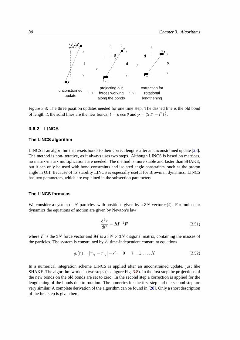
30 Chapter 3. Algorithms
����
����
������������
����
����
������������
� � � ���������������������
������������������������������������������������������
������������������������������������������������������
unconstrainedupdate
correction forrotational
lengthening
projecting outforces working
along the bonds
θ
d
l d
pd
Figure 3.8: The three position updates needed for one time step. The dashed line is the old bondof lengthd, the solid lines are the new bonds.l = d cos θ andp = (2d2 − l2)
12 .
3.6.2 LINCS
The LINCS algorithm
LINCS is an algorithm that resets bonds to their correct lengths after an unconstrained update [28].The method is non-iterative, as it always uses two steps. Although LINCS is based on matrices,no matrix-matrix multiplications are needed. The method is more stable and faster than SHAKE,but it can only be used with bond constraints and isolated angle constraints, such as the protonangle in OH. Because of its stability LINCS is especially useful for Brownian dynamics. LINCShas two parameters, which are explained in the subsection parameters.
The LINCS formulas
We consider a system ofN particles, with positions given by a3N vectorr(t). For moleculardynamics the equations of motion are given by Newton’s law
d2r
dt2= M−1F (3.51)
whereF is the3N force vector andM is a3N × 3N diagonal matrix, containing the masses ofthe particles. The system is constrained byK time-independent constraint equations
gi(r) = |ri1 − ri2 | − di = 0 i = 1, . . . ,K (3.52)
In a numerical integration scheme LINCS is applied after an unconstrained update, just likeSHAKE. The algorithm works in two steps (see figure Fig.3.8). In the first step the projections ofthe new bonds on the old bonds are set to zero. In the second step a correction is applied for thelengthening of the bonds due to rotation. The numerics for the first step and the second step arevery similar. A complete derivation of the algorithm can be found in [28]. Only a short descriptionof the first step is given here.
3.6. Constraint algorithms 31
A new notation is introduced for the gradient matrix of the constraint equations which appears onthe right hand side of the equation
Bhi =∂gh
∂ri(3.53)
Notice thatB is aK×3N matrix, it contains the directions of the constraints. The following equa-tion shows how the new constrained coordinatesrn+1 are related to the unconstrained coordinatesrunc
n+1
rn+1 = (I − T nBn)runcn+1 + T nd =
runcn+1 −M−1Bn(BnM−1BT
n )−1(Bnruncn+1 − d)
(3.54)
whereT = M−1BT (BM−1BT )−1. The derivation of this equation from eqns.3.51and3.52can be found in [28].
This first step does not set the real bond lengths to the prescribed lengths, but the projection of thenew bonds onto the old directions of the bonds. To correct for the rotation of bondi, the projectionof the bond on the old direction is set to
pi =√
2d2i − l2i (3.55)
whereli is the bond length after the first projection. The corrected positions are
r∗n+1 = (I − T nBn)rn+1 + T np (3.56)
This correction for rotational effects is actually an iterative process, but during MD only oneiteration is applied. The relative constraint deviation after this procedure will be less than 0.0001for every constraint. In energy minimization this might not be accurate enough, so the number ofiterations is equal to the order of the expansion (see below).
Half of the CPU time goes to inverting the constraint coupling matrixBnM−1BTn , which has to
be done every time step. ThisK×K matrix has1/mi1 +1/mi2 on the diagonal. The off-diagonalelements are only non-zero when two bonds are connected, then the element iscosφ/mc, wheremc is the mass of the atom connecting the two bonds andφ is the angle between the bonds.
The matrixT is inverted through a power expansion. AK ×K matrix S is introduced which isthe inverse square root of the diagonal ofBnM−1BT
n . This matrix is used to convert the diagonalelements of the coupling matrix to one
(BnM−1BTn )−1 = SS−1(BnM−1BT
n )−1S−1S
= S(SBnM−1BTnS)−1S = S(I −An)−1S
(3.57)
The matrixAn is symmetric and sparse and has zeros on the diagonal. Thus a simple trick can beused to calculate the inverse
(I −An)−1 = I + An + A2n + A3
n + . . . (3.58)
This inversion method is only valid if the absolute values of all the eigenvalues ofAn are smallerthan one. In molecules with only bond constraints the connectivity is so low that this will alwaysbe true, even if ring structures are present. Problems can arise in angle-constrained molecules. Byconstraining angles with additional distance constraints multiple small ring structures are intro-duced. This gives a high connectivity, leading to large eigenvalues. Therefore LINCS should NOTbe used with coupled angle-constraints.
32 Chapter 3. Algorithms
The LINCS Parameters
The accuracy of LINCS depends on the number of matrices used in the expansion eqn.3.58. ForMD calculations a fourth order expansion is enough. For Brownian dynamics with large time stepsan eighth order expansion may be necessary. The order is a parameter in the input file formdrun .The implementation of LINCS is done in such a way that the algorithm will never crash. Evenwhen it is impossible to to reset the constraints LINCS will generate a conformation which fulfillsthe constraints as well as possible. However, LINCS will generate a warning when in one step abond rotates over more than a predefined angle. This angle is set by the user in the input file formdrun .
3.7 Simulated Annealing
The well known simulated annealing (SA) protocol is implemented in a simple way into GRO-MACS. A modification of the temperature coupling scheme is used as a very basic implementa-tion of the SA algorithm. The method works as follows: the reference temperature for couplingT0 (eqn.3.22) is not constant but can be varied linearly:
T0(step) = T0 ∗ (λ0 + ∆λ ∗ step) (3.59)
if λ0 = 1 and∆λ is 0 this is the plain MD algorithm. Note that for standard SA∆λ must benegative. WhenT0(step)< 0 it is set to 0, as negative temperatures do not have a physical meaning.This “feature” allows for an annealing strategy in which at first the temperature is scaled downlinearly until 0 K, and when more steps are taken the simulation proceeds at 0 K. Since the weakcoupling scheme does not couple instantaneously, the actual temperature will always be slightlyhigher than 0 K.
3.8 Stochastic Dynamics
Stochastic or velocity Langevin dynamics adds a friction and a noise term to Newton’s equationsof motion:
mid2ri
dt2= −miξi
dri
dt+ F i(r)+
◦ri (3.60)
whereξi is the friction constant[1/ps] and◦ri (t) is a noise process with〈◦ri (t)
◦rj (t + s)〉 =
2miξikBTδ(s)δij . When1/ξi is large compared to the time scales present in the system, onecould see stochastic dynamics as molecular dynamics with stochastic temperature-coupling. Theadvantage compared to MD with Berendsen temperature-coupling is that in case of SD the gen-erated ensemble is known. For simulating a system in vacuum there is the additional advantagethat there is no accumulation of errors for the overall translational and rotational degrees of free-dom. When1/ξi is small compared to the time scales present in the system, the dynamics will becompletely different from MD, but the sampling is still correct.
GROMACS uses a complicated third-order leap-frog algorithm [29] to integrate equation (3.60).When constraints are present in the system, two constraint steps are performed per time step. The
3.9. Brownian Dynamics 33
kinetic energy is computed at the whole time step, this is done by averaging the velocities at minusand plus a half time step, with a correction for the friction:
v(t) =12
(v
(t− ∆t
2
)+ v
(t+
∆t2
))(e−ξ∆t +
√2(1− e−ξ∆t
))(3.61)
Exact continuation of a stochastic dynamics simulation is not possible, since apart from the coor-dinates and the velocities one random term of the previous step in required, however, the error willbe very small.
3.9 Brownian Dynamics
In the limit of high friction stochastic dynamics reduces to Brownian dynamics, also called posi-tion Langevin dynamics. This applies to over-damped systems,i.e. systems in which the inertiaeffects are negligible. The equation is:
dri
dt=
1γi
F i(r)+◦ri (3.62)
whereγi is the friction coefficient[amu/ps] and◦ri(t) is a noise process with〈◦ri(t)
◦rj(t + s)〉 =
2δ(s)δijkBT/γi. In GROMACS the equations are integrated with a simple, explicit scheme:
ri(t+ ∆t) = ri(t) +∆tγi
F i(r(t)) +
√2kBT
∆tγi
rGi (3.63)
whererGi is Gaussian distributed noise withµ = 0, σ = 1. The friction coefficientsγi can be
chosen the same for all particles or asγi = mi/ξi, where the friction constantsξi can be differentfor different groups of atoms. Because the system is assumed to be over damped, large time-stepscan be used. LINCS should be used for the constraints since SHAKE will not converge for largeatomic displacements. BD is an option of themdrun program.
3.10 Energy Minimization
Energy minimization in GROMACS can be done using a steepest descent or conjugate gradientmethod. EM is just an option of themdrun program.
3.10.1 Steepest Descent
Although steepest descent is certainly not the most efficient algorithm for searching, it is robustand easy to implement.
We define the vectorr as the vector of all3N coordinates. Initially a maximum displacementh0
(e.g.0.01 nm) must be given.
First the forcesF and potential energy are calculated. New positions are calculated by
rn+1 = rn +F n
max(|F n|)hn (3.64)
34 Chapter 3. Algorithms
wherehn is the maximum displacement andF n is the force, or the negative gradient of the poten-tial V . The notationmax(|F n|) means the largest of the absolute values of the force components.The forces and energy are again computed for the new positionsIf (Vn+1 < Vn) the new positions are accepted andhn+1 = 1.2hn.If (Vn+1 ≥ Vn) the new positions are rejected andhn = 0.2hn.
The algorithm stops when either a user specified number of force evaluations has been performed(e.g.100), or when the maximum of the absolute values of the force (gradient) components issmaller than a specified valueε. Since force truncation produces some noise in the energy evalua-tion, the stopping criterion should not be made too tight to avoid endless iterations. A reasonablevalue forε can be estimated from the root mean square forcef a harmonic oscillator would exhibitat a temperatureT This value is
f = 2πν√
2mkT (3.65)
whereν is the oscillator frequency,m the (reduced) mass, andk Boltzmann’s constant. For aweak oscillator with a wave number of 100 cm−1 and a mass of 10 atomic units, at a temperatureof 1 K, f = 7.7 kJ mol−1 nm−1. A value forε between 1 and 10 is acceptable.
3.10.2 Conjugate Gradient
Conjugate gradient is slower than steepest descent in the early stages of the minimization, butbecomes more efficient closer to the energy minimum. The parameters and stop criterion are thesame as for steepest descent. In GROMACS conjugate gradient can not be used with constraints,as this has not been implemented. This is not really a restriction, since the accuracy of conjugategradient is only required for minimization prior to a normal mode analysis, which can not beperformed with constraints. For most other purposes steepest descent is efficient enough.
3.11 Normal Mode Analysis
Normal mode analysis [30, 31, 32] can be performed using GROMACS, by diagonalization of themass-weighted HessianH:
RTM−1/2HM−1/2R = diag(λ1, . . . , λ3N ) (3.66)
λi = (2πωi)2 (3.67)
whereM contains the atomic masses,R is a matrix that contains the eigenvectors as columns,λi
are the eigenvalues andωi are the corresponding frequencies.
First the Hessian matrix, which is a3N × 3N matrix whereN is the number of atoms, needs tobe calculated:
Hij =∂2V
∂xi∂xj(3.68)
wherexi andxj denote the atomic x, y or z coordinates. In practice, this equation is not used, butthe Hessian is calculated numerically from the force as:
Hij = −fi(x + hej)− fi(x− hej)2h
(3.69)
3.12. Free energy calculations 35
fi = −∂V∂xi
(3.70)
whereej is the unit vector in directionj. It should be noted that for a usual Normal Mode calcula-tion, it is necessary to completely minimize the energy prior to computation of the Hessian. Whattolerance is required depends on the type of system, but a rough indication is 0.001 kJ mol−1. Thisshould be done with conjugate gradient in double precision.
A number of GROMACS programs are involved in these calculations. First the energy should beminimized usingmdrun . Thenmdrun computes the Hessian, note that for generating the runinput file one should use the minimized conformation from the full precision trajectory file, asthe structure file is not accurate enough.g nmeig does the diagonalization and the sorting ofthe normal modes according to their frequencies. Bothmdrun andg nmeig should be run indouble precision. The normal modes can be analyzed with the programg anaeig . Ensembles ofstructures at any temperature and for any subset of normal modes can be generated withg nmens.An overview of normal mode analysis and the related principal component analysis (see sec.8.9)can be found in [33].
3.12 Free energy calculations
Free energy calculations can be performed in GROMACS using slow-growth methods. An exam-ple problem might be: calculate the difference in free energy of binding of an inhibitorI to anenzymeE and to a mutated enzymeE′. It is not feasible with computer simulations to perform adocking calculation for such a large complex, or even releasing the inhibitor from the enzyme in areasonable amount of computer time with reasonable accuracy. However, if we consider the freeenergy cycle in (Fig.3.9A) we can write
∆G1 −∆G2 = ∆G3 −∆G4 (3.71)
If we are interested in the left-hand term we can equally well compute the right-hand term.
If we want to compute the difference in free energy of binding of two inhibitorsI and I ′ to anenzymeE (Fig. 3.9B) we can again use eqn.3.71to compute the desired property.
Free energy differences between two molecular species can be calculated in GROMACS using the“slow-growth” method. In fact, such free energy differences between different molecular speciesare physically meaningless, but they can be used to obtain meaningful quantities employing athermodynamic cycle. The method requires a simulation during which the Hamiltonian of thesystem changes slowly from that describing one system (A) to that describing the other system(B). The change must be so slow that the system remains in equilibrium during the process; if thatrequirement is fulfilled, the change is reversible and a slow-growth simulation from B to A willyield the same results (but with a different sign) as a slow-growth simulation from A to B. This isa useful check, but the user should be aware of the danger that equality of forward and backwardgrowth results does not guarantee correctness of the results.
The required modification of the HamiltonianH is realized by makingH a function of acouplingparameterλ : H = H(p, q;λ) in such a way thatλ = 0 describes system A andλ = 1 describessystem B:
H(p, q; 0) = HA(p, q); H(p, q; 1) = HB(p, q). (3.72)
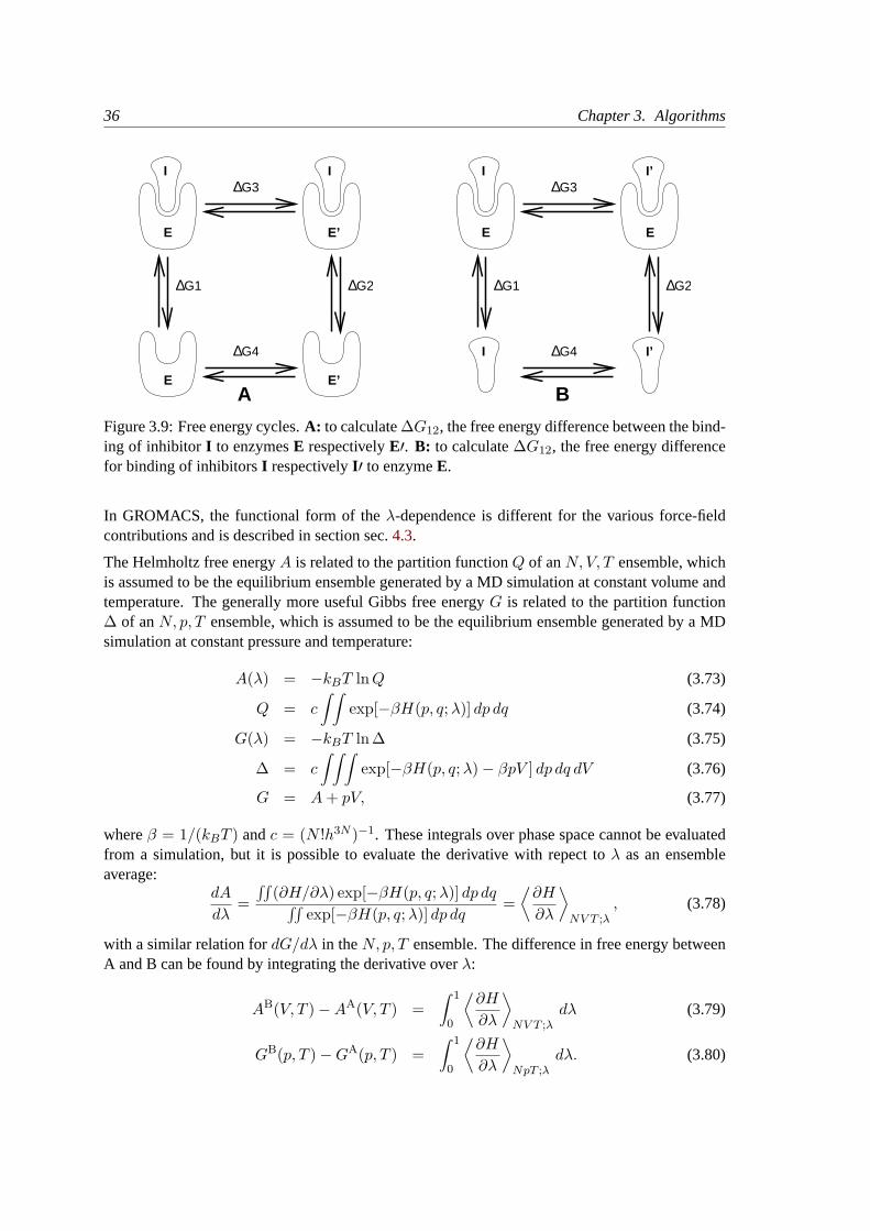
36 Chapter 3. Algorithms
I
E’E
I
E E’
G1∆ ∆G2
∆G4
∆G3
A
G1∆ ∆G2
∆G3
I I’
E
I
E
I’
∆G4
B
Figure 3.9: Free energy cycles.A: to calculate∆G12, the free energy difference between the bind-ing of inhibitor I to enzymesE respectivelyE′. B: to calculate∆G12, the free energy differencefor binding of inhibitorsI respectivelyI ′ to enzymeE.
In GROMACS, the functional form of theλ-dependence is different for the various force-fieldcontributions and is described in section sec.4.3.
The Helmholtz free energyA is related to the partition functionQ of anN,V, T ensemble, whichis assumed to be the equilibrium ensemble generated by a MD simulation at constant volume andtemperature. The generally more useful Gibbs free energyG is related to the partition function∆ of anN, p, T ensemble, which is assumed to be the equilibrium ensemble generated by a MDsimulation at constant pressure and temperature:
A(λ) = −kBT lnQ (3.73)
Q = c
∫ ∫exp[−βH(p, q;λ)] dp dq (3.74)
G(λ) = −kBT ln∆ (3.75)
∆ = c
∫ ∫ ∫exp[−βH(p, q;λ)− βpV ] dp dq dV (3.76)
G = A+ pV, (3.77)
whereβ = 1/(kBT ) andc = (N !h3N )−1. These integrals over phase space cannot be evaluatedfrom a simulation, but it is possible to evaluate the derivative with repect toλ as an ensembleaverage:
dA
dλ=∫∫
(∂H/∂λ) exp[−βH(p, q;λ)] dp dq∫∫exp[−βH(p, q;λ)] dp dq
=⟨∂H
∂λ
⟩NV T ;λ
, (3.78)
with a similar relation fordG/dλ in theN, p, T ensemble. The difference in free energy betweenA and B can be found by integrating the derivative overλ:
AB(V, T )−AA(V, T ) =∫ 1
0
⟨∂H
∂λ
⟩NV T ;λ
dλ (3.79)
GB(p, T )−GA(p, T ) =∫ 1
0
⟨∂H
∂λ
⟩NpT ;λ
dλ. (3.80)

3.13. Essential Dynamics Sampling 37
If one wishes to evaluateGB(p, T ) − GA(p, T ), the natural choice is a constant-pressure simu-lation. However, this quantity can also be obtained from a slow-growth simulation at constantvolume, starting with system A at pressurep and volumeV and ending with system B at pressurepB, by applying the following small correction:
GB(p)−GA(p) = AB(V )−AA(V )−∫ pB
p[V B(p′)− V ] dp′ (3.81)
Here we omitted the constantT from the notation. This correction is roughly equal to−12(pB −
p)∆V = (∆V )2/(2κV ), where∆V is the volume change atp andκ is the isothermal compress-ibility. This is usually negligible. For example, the growth of a water molecule from nothing in abath of 1000 water molecules at constant volume would produce an additional pressure of 22 barand a correction to the Helmholtz free energy of -20 J/mol.
In cartesian coordinates, the kinetic energy term in the Hamiltonian depends only on the momenta,and can be separately integrated and in fact removed from the equations. When masses do notchange, there is no contribution from the kinetic energy at all; otherwise the integrated contributionto the free energy is−3
2kBT ln(mB/mA). This is no longer true in the presence of constraints.
GROMACS offers the possibility to integrate eq.3.79or eq. 3.80in one simulation over the fullrange from A to B. However, if the change is large and sampling insufficiency can be expected,the user may prefer to determine the value of〈dG/dλ〉 accurately at a number of well-chosenintermediate values ofλ. This can be easily done by setting the stepsizedelta lambda to zero.Each simulation can be equilibrated first, and a proper error estimate can be made for each value ofdG/dλ from the fluctuation of∂H/∂λ. The total free energy change is then determined afterwardsby an appropriate numerical integration procedure.
Theλ-dependence for the force-field contributions is described in section sec.4.3.
3.13 Essential Dynamics Sampling
The results from Essential Dynamics (see sec.8.9) of a protein can be used to guide MD simula-tions. The idea is that from an initial MD simulation (or from other sources) a definition of thecollective fluctuations with largest amplitude is obtained. The position along one or more of thesecollective modes can be constrained in a (second) MD simulation in a number of ways for severalpurposes. For example, the position along a certain mode may be kept fixed to monitor the averageforce (free-energy gradient) on that coordinate in that position. Another application is to enhancesampling efficiency with respect to usual MD [34, 35]. In this case, the system is encouragedto sample its available configuration space more systematically than in a diffusion-like path thatproteins usually take.
All available constraint types are described in the appropriate chapter of the WHAT IF [36] man-ual.
38 Chapter 3. Algorithms
3.14 Parallelization
The purpose of this section is to discuss the parallelization of the principle MD algorithm and not todescribe the algorithms that are in practical use for molecular systems with their complex variety ofatoms and terms in the force field descriptions. We shall therefore consider as an example a simplesystem consisting only of a single type of atoms with a simple form of the interaction potential.The emphasis will be on the special problems that arise when the algorithm is implemented on aparallel computer.
The simple model problem already contains the bottleneck of all MD simulations: the compu-tationally intensive evaluation of thenon-bondedforces between pairs of atoms, based on thedistance between particles. Complex molecular systems will in addition involve many differentkinds ofbondedforces between designated atoms. Such interactions add to the complexity of thealgorithm but do not modify the basic considerations concerning parallelization.
3.14.1 Methods of parallelization
There are a number of methods to parallelize the MD algorithm, each of them with their ownadvantages and disadvantages. The method to choose depends on the hardware and compilersavailable. We list them here:
1 Message Passing.In this method, which is more or less the traditional way of parallel programming, all theparallelism is explicitly programmed by the user. The disadvantage is that it takes extra codeand effort, the advantage is that the programmer keeps full control over the data flow andcan do optimizations a compiler could not come up with.
The implementation is typically done by calling a set of library routines to send and re-ceive data to and from other processors. Almost all hardware vendors support this way ofparallelism in their C and Fortran compilers.
2 Data Parallel.This method lets the user define arrays on which to operate in parallel. Programming thisway is much like vectorizing: recurrence is not parallelized (e.g.for(i=1; (i<MAX);i++) a[i] = a[i-1] + 1; does not vectorize and not parallelize, because for everyi the result from the previous step is needed).
The advantage of data parallelism is that it is easier for the user; the compiler takes care ofthe parallelism. The disadvantage is that it is supported by a small (though growing) numberof hardware vendors, and that it is much harder to maintain a program that has to run onboth parallel and sequential machines, because the only standard language that supports itis Fortran-90 which is not available on many platforms.
Both methods allow for the MD algorithm to be implemented without much trouble. Messagepassing MD algorithms have been published since the mid 80’s ([37], [38]) and development isstill continuing. Data parallel programming is newer, but starting from a well vectorized programit is not hard to do.
3.14. Parallelization 39
Our implementation of MD is a message passing one, the reason for which is partly historical:the project to develop a parallel MD program started when Fortran-90 was still in the making,and no compilers were expected to be available. At current, we still believe that message passingis the way to go, after having done some experiments with data parallel programming on a Con-nection Machine (CM-5), because of portability to other hardware, the poor performance of thecode produced by the compilers and because this way of programming has the same drawback asvectorization: the part of the program that is not vectorized or parallelized determines the runtimeof the program (Amdahl’s law).
The approach we took to parallelism was a minimalist one: use as few non-standard elements inthe software as possible, and use the simplest processor topology that does the job. We thereforedecided to use a standard language (ANSI-C) with as few non-standard routines as possible. Weonly use 5 communication routines that are non-standard. It is therefore very easy to port our codeto other machines.
For anO(N2) problem like MD, one of the best schemes for the interprocessor connections is aring, so our software demands that a ring is present in the interprocessor connections. A ring canessentially always be mapped onto another network like a hypercube, a bus interface (Ethernete.g.using Message Passing Interface MPI) or a tree (CM-5). Some hardware vendors have veryluxurious connection schemes that connect every processor to every other processor, but we do notreally need it and so do not use it even though it might come in handy at times. The advantage withthis simple scheme is that GROMACS performs extremely well even on inexpensive workstationclusters.
When using a message passing scheme one has to divide the particles over processors, which canbe done in two ways:
• Space Decomposition.An element of space is allocated to each processor, when dividing a cubic box with edgeb overP processors this can be done by giving each processor a slab of lengthb/P . Thismethod has the advantage that each processor has about the same number of interactions tocalculate (at least when the simulated system has a homogeneous density, like a liquid or agas). The disadvantage is that a lot of bookkeeping is necessary for particles that move overprocessor boundaries. When using more complex systems, such as macromolecules thereare also 3- and 4-atom interactions that make the bookkeeping too complicated for our taste.
• Particle Decomposition.Every processor is allocated a number of particles. When dividingN particles overPprocessors each processor will getN/P particles. The implementation of this method isdescribed in the next section.
3.14.2 MD on a ring of processors
When a neighbor list is not used the MD problem is in principle anO(N2) problem as each particlecan interact with every other. This can be simplified using Newton’s third law
Fij = − Fji (3.82)
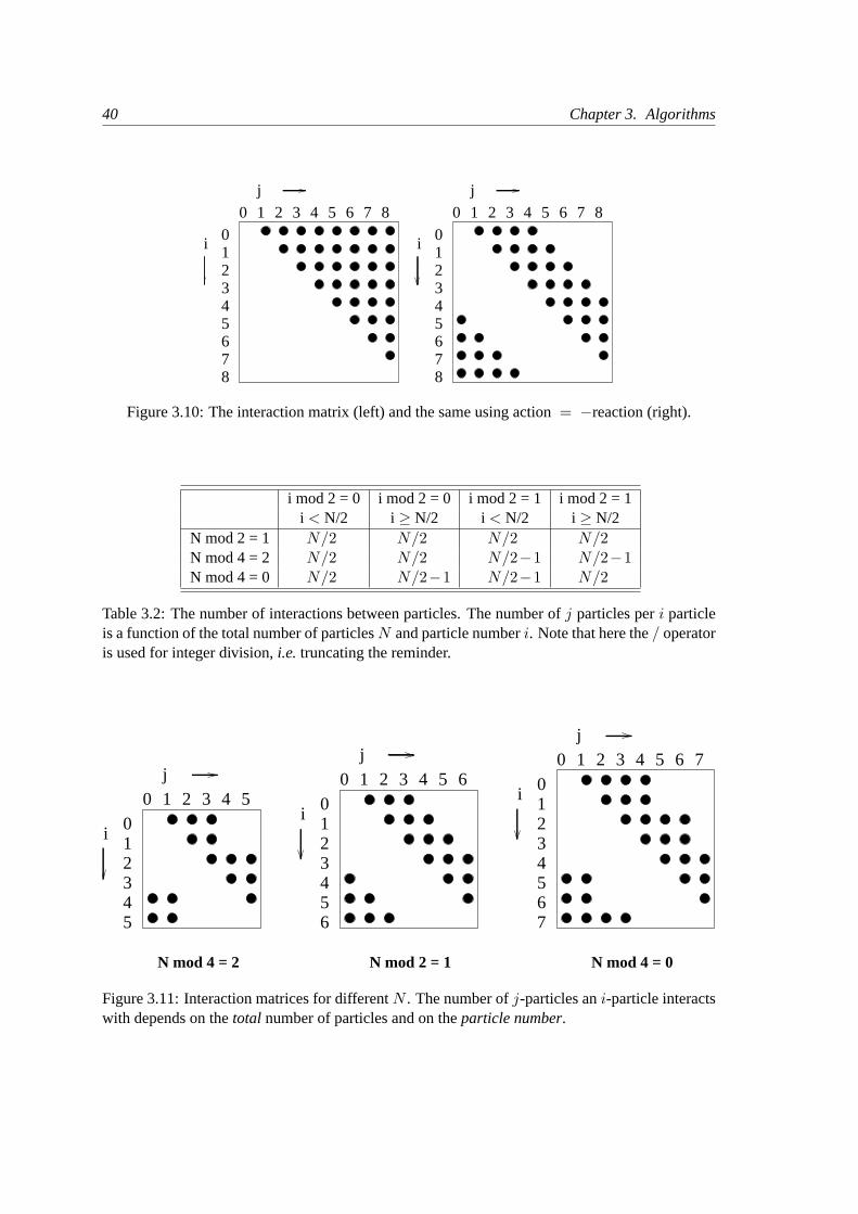
40 Chapter 3. Algorithms
012345678
012345678
0 1 2 3 4 5 6 7 8 0 1 2 3 4 5 6 7 8j j
i i
Figure 3.10: The interaction matrix (left) and the same using action= −reaction (right).
i mod 2 = 0 i mod 2 = 0 i mod 2 = 1 i mod 2 = 1i < N/2 i ≥ N/2 i < N/2 i ≥ N/2
N mod 2 = 1 N/2 N/2 N/2 N/2N mod 4 = 2 N/2 N/2 N/2−1 N/2−1N mod 4 = 0 N/2 N/2−1 N/2−1 N/2
Table 3.2: The number of interactions between particles. The number ofj particles peri particleis a function of the total number of particlesN and particle numberi. Note that here the/ operatoris used for integer division,i.e. truncating the reminder.
j
i
j
i
j
i012345
0 1 2 3 4 501234567
0 1 2 3 4 5 6 7
0123456
0 1 2 3 4 5 6
N mod 4 = 2 N mod 2 = 1 N mod 4 = 0
Figure 3.11: Interaction matrices for differentN . The number ofj-particles ani-particle interactswith depends on thetotal number of particles and on theparticle number.
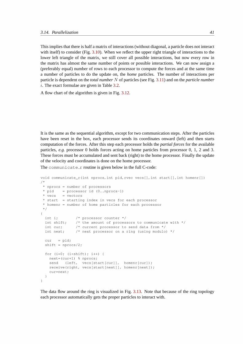
3.14. Parallelization 41
This implies that there is half a matrix of interactions (without diagonal, a particle does not interactwith itself) to consider (Fig.3.10). When we reflect the upper right triangle of interactions to thelower left triangle of the matrix, we still cover all possible interactions, but now every row inthe matrix has almost the same number of points or possible interactions. We can now assign a(preferably equal) number of rows to each processor to compute the forces and at the same timea number of particles to do the update on, thehomeparticles. The number of interactions perparticle is dependent on thetotal numberN of particles (see Fig.3.11) and on theparticle numberi. The exact formulae are given in Table3.2.
A flow chart of the algorithm is given in Fig.3.12.
It is the same as the sequential algorithm, except for two communication steps. After the particleshave been reset in the box, each processor sends its coordinates onward (left) and then startscomputation of the forces. After this step each processor holds thepartial forcesfor the availableparticles,e.g. processor 0 holds forces acting on home particles from processor 0, 1, 2 and 3.These forces must be accumulated and sent back (right) to the home processor. Finally the updateof the velocity and coordinates is done on the home processor.
Thecommunicate r routine is given below in the full C-code:
void communicate_r(int nprocs,int pid,rvec vecs[],int start[],int homenr[])/*
* nprocs = number of processors* pid = processor id (0..nprocs-1)* vecs = vectors* start = starting index in vecs for each processor* homenr = number of home particles for each processor*/
{int i; /* processor counter */int shift; /* the amount of processors to communicate with */int cur; /* current processor to send data from */int next; /* next processor on a ring (using modulo) */
cur = pid;shift = nprocs/2;
for (i=0; (i<shift); i++) {next=(cur+1) % nprocs;send (left, vecs[start[cur]], homenr[cur]);receive(right, vecs[start[next]], homenr[next]);cur=next;
}}
The data flow around the ring is visualized in Fig.3.13. Note that because of the ring topologyeach processor automatically gets the proper particles to interact with.
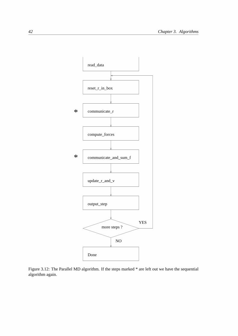
42 Chapter 3. Algorithms
read_data
Done
NO
output_step
update_r_and_v
more steps ?YES
compute_forces
*
*
reset_r_in_box
communicate_r
communicate_and_sum_f
Figure 3.12: The Parallel MD algorithm. If the steps marked * are left out we have the sequentialalgorithm again.
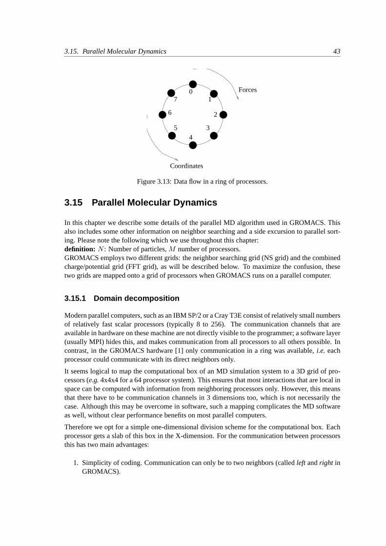
3.15. Parallel Molecular Dynamics 43
01
2
34
5
6
7Forces
Coordinates
Figure 3.13: Data flow in a ring of processors.
3.15 Parallel Molecular Dynamics
In this chapter we describe some details of the parallel MD algorithm used in GROMACS. Thisalso includes some other information on neighbor searching and a side excursion to parallel sort-ing. Please note the following which we use throughout this chapter:definition: N : Number of particles,M number of processors.GROMACS employs two different grids: the neighbor searching grid (NS grid) and the combinedcharge/potential grid (FFT grid), as will be described below. To maximize the confusion, thesetwo grids are mapped onto a grid of processors when GROMACS runs on a parallel computer.
3.15.1 Domain decomposition
Modern parallel computers, such as an IBM SP/2 or a Cray T3E consist of relatively small numbersof relatively fast scalar processors (typically 8 to 256). The communication channels that areavailable in hardware on these machine are not directly visible to the programmer; a software layer(usually MPI) hides this, and makes communication from all processors to all others possible. Incontrast, in the GROMACS hardware [1] only communication in a ring was available,i.e. eachprocessor could communicate with its direct neighbors only.
It seems logical to map the computational box of an MD simulation system to a 3D grid of pro-cessors (e.g.4x4x4 for a 64 processor system). This ensures that most interactions that are local inspace can be computed with information from neighboring processors only. However, this meansthat there have to be communication channels in 3 dimensions too, which is not necessarily thecase. Although this may be overcome in software, such a mapping complicates the MD softwareas well, without clear performance benefits on most parallel computers.
Therefore we opt for a simple one-dimensional division scheme for the computational box. Eachprocessor gets a slab of this box in the X-dimension. For the communication between processorsthis has two main advantages:
1. Simplicity of coding. Communication can only be to two neighbors (calledleft andright inGROMACS).
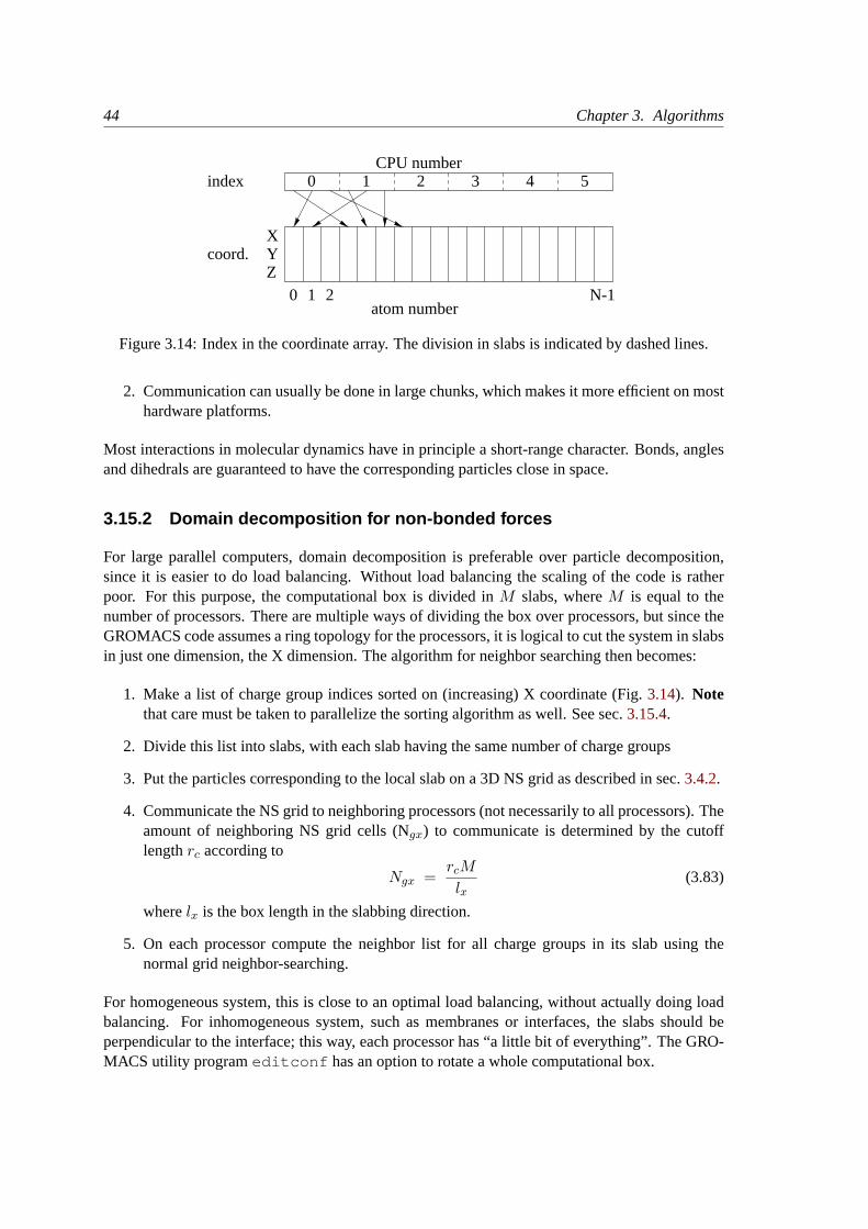
44 Chapter 3. Algorithms
XYZ
0 1 2 N-1
0 1 2 3 4 5CPU number
atom number
index
coord.
Figure 3.14: Index in the coordinate array. The division in slabs is indicated by dashed lines.
2. Communication can usually be done in large chunks, which makes it more efficient on mosthardware platforms.
Most interactions in molecular dynamics have in principle a short-range character. Bonds, anglesand dihedrals are guaranteed to have the corresponding particles close in space.
3.15.2 Domain decomposition for non-bonded forces
For large parallel computers, domain decomposition is preferable over particle decomposition,since it is easier to do load balancing. Without load balancing the scaling of the code is ratherpoor. For this purpose, the computational box is divided inM slabs, whereM is equal to thenumber of processors. There are multiple ways of dividing the box over processors, but since theGROMACS code assumes a ring topology for the processors, it is logical to cut the system in slabsin just one dimension, the X dimension. The algorithm for neighbor searching then becomes:
1. Make a list of charge group indices sorted on (increasing) X coordinate (Fig.3.14). Notethat care must be taken to parallelize the sorting algorithm as well. See sec.3.15.4.
2. Divide this list into slabs, with each slab having the same number of charge groups
3. Put the particles corresponding to the local slab on a 3D NS grid as described in sec.3.4.2.
4. Communicate the NS grid to neighboring processors (not necessarily to all processors). Theamount of neighboring NS grid cells (Ngx) to communicate is determined by the cutofflengthrc according to
Ngx =rcM
lx(3.83)
wherelx is the box length in the slabbing direction.
5. On each processor compute the neighbor list for all charge groups in its slab using thenormal grid neighbor-searching.
For homogeneous system, this is close to an optimal load balancing, without actually doing loadbalancing. For inhomogeneous system, such as membranes or interfaces, the slabs should beperpendicular to the interface; this way, each processor has “a little bit of everything”. The GRO-MACS utility programeditconf has an option to rotate a whole computational box.
3.15. Parallel Molecular Dynamics 45
The following observations are important here:
• Particles may diffuse from one slab to the other, therefore each processor must hold coordi-nates for all particles all the time, and distribute forces back to all processors as well.
• Velocities are kept on the “home processor” for each particle, where the integration of New-ton’s equations is done.
• Fixed interaction lists (bonds, angles etc.) are kept each on a single processor. Since allprocessors have all coordinates, it does not matter where interactions are calculated. Thedivision is actually done by the GROMACS preprocessorgrompp and care is taken that, asfar as possible, every processor gets the same number of bonded interactions.
In all, this makes for a mixed particle decomposition/domain decomposition scheme for paral-lelization of the MD code. The communication costs are four times higher than for the simpleparticle decomposition method described in sec.3.14 (the whole coordinate and force array arecommunicated across the whole ring, rather than half the array over half the ring). However, forlarge numbers of processors the improved load balancing compensates this easily.
3.15.3 Parallel PPPM
A further reason for domain decomposition is the PPPM algorithm. This algorithm works witha 3D Fast Fourier Transform. It employs a discrete grid of dimensions (nx,ny,nz), the FFT grid.The algorithm consist of five steps, each of which have to be parallelized:
1. Spreading charges on the FFT grid to obtain the charge distributionρ(r). This bit involvesthe following sub-steps:
a. put particle in the box
b. find the FFT grid cell in which the particle resides
c. add the charge of the particle times the appropriate weight factor (see sec.4.6.3) toeach of the 27 grid points (3 x 3 x 3).
In the parallel case, the FFT grid must be filled on each processor with its share of the par-ticles, and subsequently the FFT grids of all processors must be summed to find the totalcharge distribution. It may be clear that this induces a large amount of unnecessary work,unless we use domain decomposition. If each processor only has particles in a certain re-gion of space, it only has to calculate the charge distribution for that region of space. SinceGROMACS works with slabs, this means that each processor fills the FFT grid cells corre-sponding to it’s slab in space and addition of FFT grids need only be done for neighboringslabs.To be more precise, the slabx for processori is defined as:
ilxM
≤ x < (i+ 1)lxM
(3.84)
46 Chapter 3. Algorithms
Particle with thisx coordinate range will add to the charge distribution on the followingrange of of FFT grid slabs in thex direction:
trunc(ilxnx
M
)− 1 ≤ ix ≤ trunc
((i+ 1)
lxnx
M
)+ 2 (3.85)
where trunc indicates the truncation of a real number to the largest integer smaller than orequal to that real number.
2. Doing the Fourier transform of the charge distributionρ(r) in parallel to obtainρ(k). Thisis done using the FFTW library (seewww.fftw.org) which employs the MPI library formessage passing programs (note that there are also shared memory versions of the FFTWcode).This FFT algorithm actually use slabs as well (good thinking!). Each processor does 2DFFTs on its slab, and then the whole FFT grid is transposedin place(i.e.without using extramemory). This means that after the FFT the X and Y components are swapped. To completethe FFT, this swapping should be undone in principle (by transposing back). Happily theFFTW code has an option to omit this, which we use in the next step.
3. Convoluteρ(k) with the Fourier transform of the charge spread functiong(k) (which wehave tabulated before) to obtain the potentialφ(k). As an optimization, we store theg(k)in transposed form as well, matching the transposed form ofρ(k) which we get from theFFTW routine. After this step we have the potentialφ(k) in Fourier space, but still on thetransposed FFT grid.
4. Do an inverse transform ofφ(k) to obtainφ(r). Since the algorithm must do a transpose ofthe data this step actually yields the wanted result: the un-transposed potential in real space.
5. Interpolate the potentialφ(r) in real space at the particle positions to obtain forces andenergy. For this bit the same considerations about parallelism hold as for the charge spread-ing. However in this case more neighboring grid cells are needed, implying that we needthe following set of FFT grid slabs in thex direction:
trunc(ilxnx
M
)− 3 ≤ ix ≤ trunc
((i+ 1)
lxnx
M
)+ 4 (3.86)
The algorithm as sketched above requires communication for spreading the charges, for the for-ward and backward FFTs, and for interpolating the forces. The GROMACS bits of the programuse only left and right communication,i.e. using two communication channels. The FFTW rou-tines actually use other forms of communication as well, and these routines are coded with MPIroutines for message passing. This implies that GROMACS can only perform the PPPM algo-rithm on parallel computers that support MPI. However, most shared memory computers, such asthe SGI Origin, also support MPI using the shared memory for communication.
3.15.4 Parallel sorting
For the domain decomposition bit of GROMACS it is necessary to sort the coordinates (or ratherthe index to coordinates) every time a neighbor list is made. If we use brute force, and sort all co-ordinates on each processor (which is technically possible since we have all the coordinates), then

3.15. Parallel Molecular Dynamics 47
this sorting procedure will take a constant wallclock time, proportional toN2 logN , regardless ofthe number of processors. We can however do a little better, if we assume that particles diffuseonly slowly. A parallel sorting algorithm can be conceived as follows:At the first step of the simulation
1. Do a full sort of all indices usinge.g.the Quicksort algorithm that is built-in in the standardC-library
2. Divide the sorted array into slabs (as described above see Fig.3.14).
At subsequent steps of the simulation:
1. Send the indices for each processor to the preceding processor (if not processor 0) andto the next processor (if notM -1). The communication associated with this operation isproportional to 2N /M .
2. Sort the combined indices of the three (or two) processors. Note that the CPU time associ-ated with sorting is now (3N /M )2 log (3N /M ).
3. On each processor, the indices belonging to it’s slab can be determined from the order ofthe array (Fig.3.14).

48 Chapter 3. Algorithms
Chapter 4
Force fields
A force field is built up from two distinct components:
• The set of equations (called thepotential functions) used to generate the potential energiesand their derivatives, the forces.
• The parameters used in this set of equations
Within one set of equations various sets of parameters can be used. Care must be taken that thecombination of equations and parameters form a consistent set. It is in general dangerous to makead hocchanges in a subset of parameters, because the various contributions to the total force areusually interdependent.
GROMACS 3.1.1 includes two GROMACS force fields and three GROMOS forcefields. TheGROMACS forcefields are based on GROMOS-87 [39], with a small modification concerning theinteraction between water-oxygens and carbon atoms [40, 41], as well as 10 extra atom types [42,43, 40, 41, 44]. However, the user is free to make her own modifications (beware!). This will beexplained in details in chapter5, which deals with theTopology. The organization of the forcefield files is described in sec.5.7.
To accommodate the potential functions used in some popular force fields, GROMACS offersa choice of functions, both for non-bonded interaction and for dihedral interactions. They aredescribed in the appropriate subsections.
The potential functions can be subdivided into three parts
1. Non-bonded: Lennard-Jones or Buckingham, and Coulomb or modified Coulomb. The non-bonded interactions are computed on the basis of a neighbor list (a list of non-bonded atomswithin a certain radius), in which exclusions are already removed.
2. Bonded: covalent bond-stretching, angle-bending, improper dihedrals, and proper dihedrals.These are computed on the basis of fixed lists.
3. Special: position restraints and distance restraints, based on fixed lists.
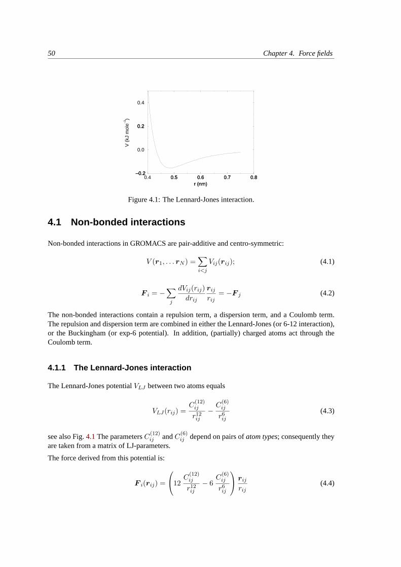
50 Chapter 4. Force fields
0.4 0.5 0.6 0.7 0.8r (nm)
–0.2
0.0
0.2
0.4
V (
kJ m
ole–1
)
Figure 4.1: The Lennard-Jones interaction.
4.1 Non-bonded interactions
Non-bonded interactions in GROMACS are pair-additive and centro-symmetric:
V (r1, . . . rN ) =∑i<j
Vij(rij); (4.1)
F i = −∑j
dVij(rij)drij
rij
rij= −F j (4.2)
The non-bonded interactions contain a repulsion term, a dispersion term, and a Coulomb term.The repulsion and dispersion term are combined in either the Lennard-Jones (or 6-12 interaction),or the Buckingham (or exp-6 potential). In addition, (partially) charged atoms act through theCoulomb term.
4.1.1 The Lennard-Jones interaction
The Lennard-Jones potentialVLJ between two atoms equals
VLJ(rij) =C
(12)ij
r12ij
−C
(6)ij
r6ij(4.3)
see also Fig.4.1The parametersC(12)ij andC(6)
ij depend on pairs ofatom types; consequently theyare taken from a matrix of LJ-parameters.
The force derived from this potential is:
F i(rij) =
12C
(12)ij
r12ij
− 6C
(6)ij
r6ij
rij
rij(4.4)
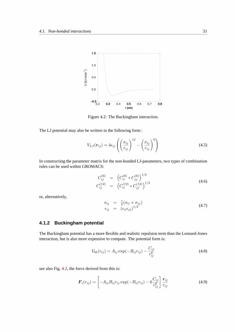
4.1. Non-bonded interactions 51
0.2 0.3 0.4 0.5 0.6 0.7 0.8r (nm)
–0.5
0.0
0.5
1.0
1.5
V (
kJ m
ole–1
)
Figure 4.2: The Buckingham interaction.
The LJ potential may also be written in the following form :
VLJ(rij) = 4εij
(σij
rij
)12
−(σij
rij
)6 (4.5)
In constructing the parameter matrix for the non-bonded LJ-parameters, two types of combinationrules can be used within GROMACS:
C(6)ij =
(C
(6)ii ∗ C(6)
jj
)1/2
C(12)ij =
(C
(12)ii ∗ C(12)
jj
)1/2 (4.6)
or, alternatively,σij = 1
2(σii + σjj)εij = (εiiεjj)
1/2 (4.7)
4.1.2 Buckingham potential
The Buckingham potential has a more flexible and realistic repulsion term than the Lennard-Jonesinteraction, but is also more expensive to compute. The potential form is:
Vbh(rij) = Aij exp(−Bijrij)−Cij
r6ij(4.8)
see also Fig.4.2, the force derived from this is:
F i(rij) =
[−AijBijrij exp(−Bijrij)− 6
Cij
r6ij
]rij
rij(4.9)
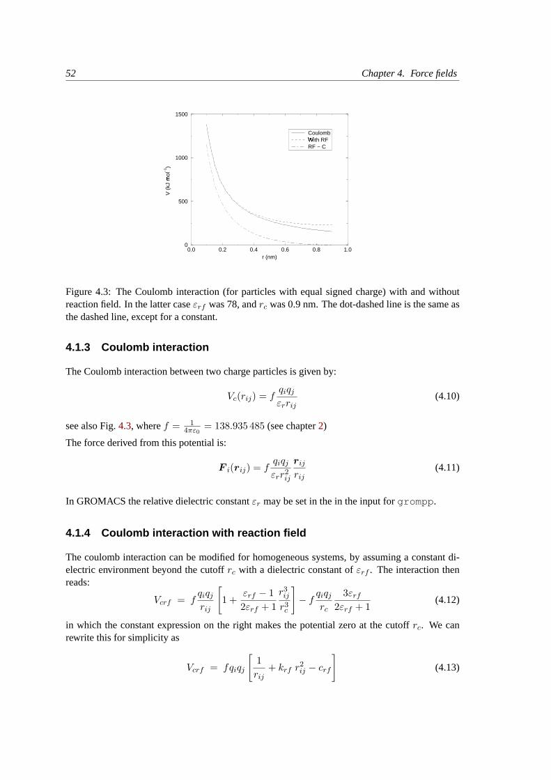
52 Chapter 4. Force fields
0.0 0.2 0.4 0.6 0.8 1.0r (nm)
0
500
1000
1500
V (
kJ m
ol�
−1 )
CoulombWith RF
�
RF − C
Figure 4.3: The Coulomb interaction (for particles with equal signed charge) with and withoutreaction field. In the latter caseεrf was 78, andrc was 0.9 nm. The dot-dashed line is the same asthe dashed line, except for a constant.
4.1.3 Coulomb interaction
The Coulomb interaction between two charge particles is given by:
Vc(rij) = fqiqjεrrij
(4.10)
see also Fig.4.3, wheref = 14πε0
= 138.935 485 (see chapter2)
The force derived from this potential is:
F i(rij) = fqiqjεrr2ij
rij
rij(4.11)
In GROMACS the relative dielectric constantεr may be set in the in the input forgrompp .
4.1.4 Coulomb interaction with reaction field
The coulomb interaction can be modified for homogeneous systems, by assuming a constant di-electric environment beyond the cutoffrc with a dielectric constant ofεrf . The interaction thenreads:
Vcrf = fqiqjrij
[1 +
εrf − 12εrf + 1
r3ijr3c
]− f
qiqjrc
3εrf
2εrf + 1(4.12)
in which the constant expression on the right makes the potential zero at the cutoffrc. We canrewrite this for simplicity as
Vcrf = fqiqj
[1rij
+ krf r2ij − crf
](4.13)
4.1. Non-bonded interactions 53
with
krf =1r3c
εrf − 1(2εrf + 1)
(4.14)
crf =1rc
+ krf r2c =
1rc
3εrf
(2εrf + 1)(4.15)
For largeεrf the krf goes to 0.5r−3c , while for εrf = 1 the correction vanishes. This makes it
possible to use the same expression with and without reaction field, albeit at some computationalcost. In Fig.4.3 the modified interaction is plotted, and it is clear that the derivative with respectto rij (= -force) goes to zero at the cutoff distance. The force derived from this potential reads:
F i(rij) = fqiqj
[1r2ij
− 2krfrij
]rij
rij(4.16)
Tironi et al. have introduced a generalized reaction field in which the dielectric continuum beyondthe cutoffrc also has an ionic strengthI [45]. In this case we can rewrite the constantskrf andcrf using the inverse Debye screening lengthκ:
κ =2I F 2
ε0εrfRT=
F 2
ε0εrfRT
K∑i=1
cizi (4.17)
krf =1r3c
(εrf − 1)(1 + κrc) + εrf (κrc)2
(2εrf + 1)(1 + κrc) + 2εrf (κrc)2(4.18)
crf =1rc
3εrf (1 + κrc + (κrc)2)(2εrf + 1)(1 + κrc) + 2εrf (κrc)2
(4.19)
whereF is Faraday’s constant,R is the ideal gas constant,T the absolute temperature,ci themolar concentration for speciesi andzi the charge number of speciesi where we haveK differentspecies. In the limit of zero ionic strength (κ = 0) eqns.4.18and4.19reduce to the simple formsof eqns.4.14and4.15respectively.
4.1.5 Modified non-bonded interactions
In the GROMACS force field the non-bonded potentials can be modified by a shift function. Thepurpose of this is to replace the truncated forces by forces that are continuous and have continuousderivatives at the cutoff radius. With such forces the time-step integration produces much smallererrors and there are no such complications as creating charges from dipoles by the truncationprocedure. In fact, by using shifted forces there is no need for charge groups in the construction ofneighbor lists. However, the shift function produces a considerable modification of the Coulombpotential. Unless the ’missing’ long-range potential is properly calculated and added (through theuse of PPPM, Ewald, or PME), the effect of such modifications must be carefully evaluated. Themodification of the Lennard-Jones dispersion and repulsion is only minor, but it does remove thenoise caused by cutoff effects.
There isno fundamental difference between a switch function (which multiplies the potential witha function) and a shift function (which adds a function to the force or potential). The switch
54 Chapter 4. Force fields
function is a special case of the shift function, which we apply to theforce functionF (r), relatedto the electrostatic or Van der Waals force acting on particlei by particlej as
F i = cF (rij)rij
rij(4.20)
For pure Coulomb or Lennard-Jones interactionsF (r) = Fα(r) = r−(α+1). The shifted forceFs(r) can generally be written as:
Fs(r) = Fα(r) r < r1
Fs(r) = Fα(r) + S(r) r1 ≤ r < rc
Fs(r) = 0 rc ≤ r
(4.21)
When r1 = 0 this is a traditional shift function, otherwise it acts as a switch function. Thecorresponding shifted coulomb potential then reads:
Vs(rij) = fΦs(rij)qiqj (4.22)
whereΦ(r) is the potential function
Φs(r) =∫ ∞
rFs(x) dx (4.23)
The GROMACS shift function should be smooth at the boundaries, therefore the following bound-ary conditions are imposed on the shift function:
S(r1) = 0S′(r1) = 0S(rc) = −Fα(rc)S′(rc) = −F ′α(rc)
(4.24)
A 3rd degree polynomial of the form
S(r) = A(r − r1)2 +B(r − r1)3 (4.25)
fulfills these requirements. The constants A and B are given by the boundary condition atrc:
A = −(α+ 4)rc − (α+ 1)r1rα+2c (rc − r1)2
B =(α+ 3)rc − (α+ 1)r1
rα+2c (rc − r1)3
(4.26)
Thus the total force function is
Fs(r) =1
rα+1+A(r − r1)2 +B(r − r1)3 (4.27)
and the potential function reads
Φ(r) =1rα
− A
3(r − r1)3 −
B
4(r − r1)4 − C (4.28)
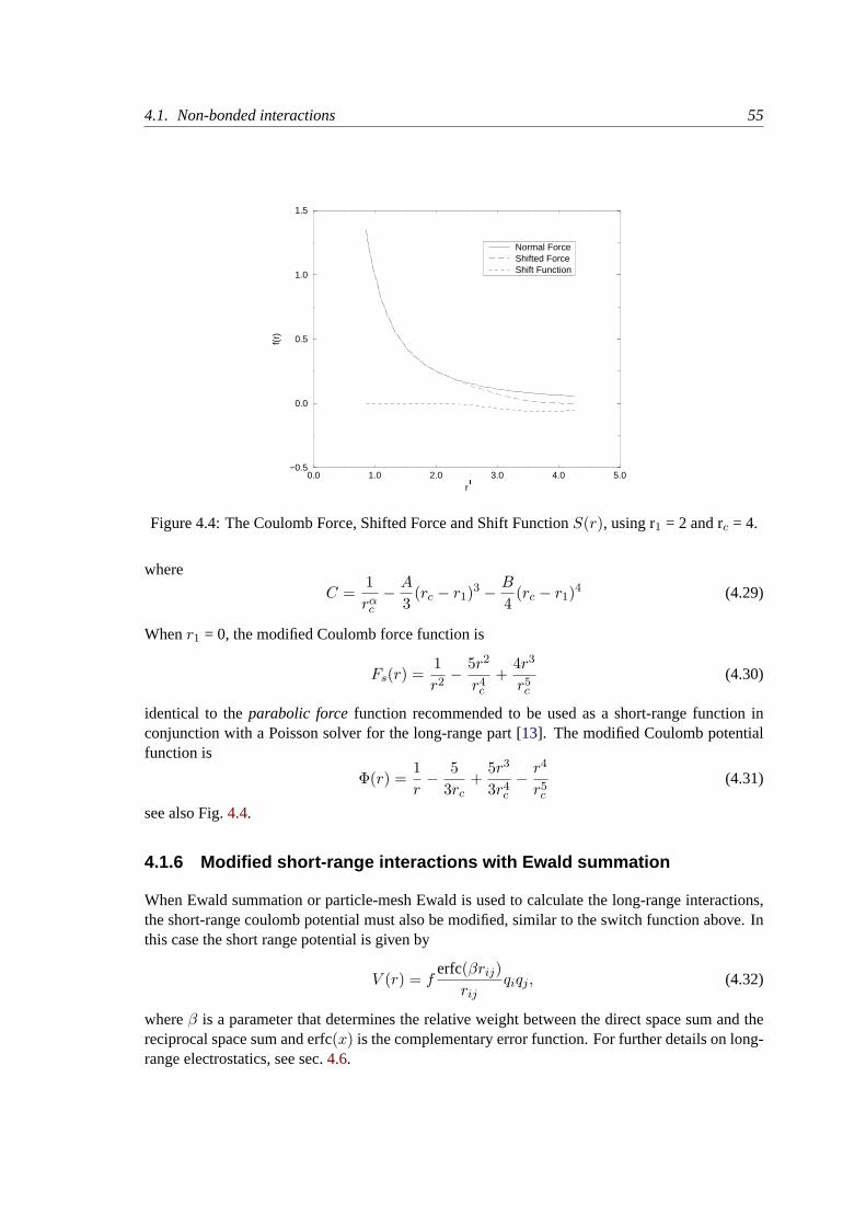
4.1. Non-bonded interactions 55
0.0 1.0 2.0 3.0 4.0 5.0r�
−0.5
0.0
0.5
1.0
1.5
f(r)
Normal ForceShifted ForceShift Function
Figure 4.4: The Coulomb Force, Shifted Force and Shift FunctionS(r), using r1 = 2 and rc = 4.
where
C =1rαc
− A
3(rc − r1)3 −
B
4(rc − r1)4 (4.29)
Whenr1 = 0, the modified Coulomb force function is
Fs(r) =1r2− 5r2
r4c+
4r3
r5c(4.30)
identical to theparabolic forcefunction recommended to be used as a short-range function inconjunction with a Poisson solver for the long-range part [13]. The modified Coulomb potentialfunction is
Φ(r) =1r− 5
3rc+
5r3
3r4c− r4
r5c(4.31)
see also Fig.4.4.
4.1.6 Modified short-range interactions with Ewald summation
When Ewald summation or particle-mesh Ewald is used to calculate the long-range interactions,the short-range coulomb potential must also be modified, similar to the switch function above. Inthis case the short range potential is given by
V (r) = ferfc(βrij)
rijqiqj , (4.32)
whereβ is a parameter that determines the relative weight between the direct space sum and thereciprocal space sum and erfc(x) is the complementary error function. For further details on long-range electrostatics, see sec.4.6.
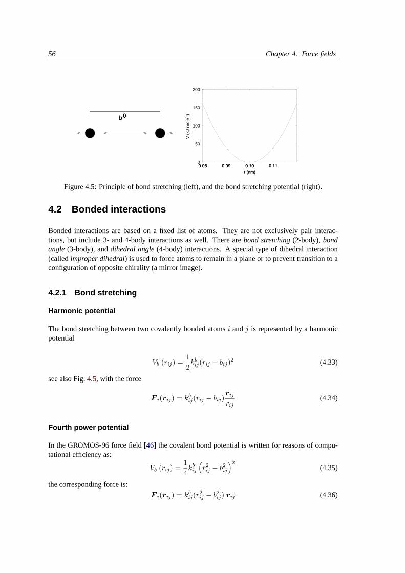
56 Chapter 4. Force fields
b0
0.08 0.09 0.10 0.11r (nm)
0
50
100
150
200
V (
kJ m
ole–1
)Figure 4.5: Principle of bond stretching (left), and the bond stretching potential (right).
4.2 Bonded interactions
Bonded interactions are based on a fixed list of atoms. They are not exclusively pair interac-tions, but include 3- and 4-body interactions as well. There arebond stretching(2-body),bondangle(3-body), anddihedral angle(4-body) interactions. A special type of dihedral interaction(calledimproper dihedral) is used to force atoms to remain in a plane or to prevent transition to aconfiguration of opposite chirality (a mirror image).
4.2.1 Bond stretching
Harmonic potential
The bond stretching between two covalently bonded atomsi andj is represented by a harmonicpotential
Vb (rij) =12kb
ij(rij − bij)2 (4.33)
see also Fig.4.5, with the force
F i(rij) = kbij(rij − bij)
rij
rij(4.34)
Fourth power potential
In the GROMOS-96 force field [46] the covalent bond potential is written for reasons of compu-tational efficiency as:
Vb (rij) =14kb
ij
(r2ij − b2ij
)2(4.35)
the corresponding force is:
F i(rij) = kbij(r
2ij − b2ij) rij (4.36)
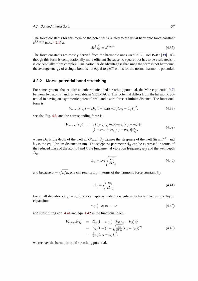
4.2. Bonded interactions 57
The force constants for this form of the potential is related to the usual harmonic force constantkb,harm (sec.4.2.1) as
2kbb2ij = kb,harm (4.37)
The force constants are mostly derived from the harmonic ones used in GROMOS-87 [39]. Al-though this form is computationally more efficient (because no square root has to be evaluated), itis conceptually more complex. One particular disadvantage is that since the form is not harmonic,the average energy of a single bond is not equal to1
2kT as it is for the normal harmonic potential.
4.2.2 Morse potential bond stretching
For some systems that require an anharmonic bond stretching potential, the Morse potential [47]between two atomsi andj is available in GROMACS. This potential differs from the harmonic po-tential in having an asymmetric potential well and a zero force at infinite distance. The functionalform is:
Vmorse(rij) = Dij [1− exp(−βij(rij − bij))]2, (4.38)
see also Fig.4.6, and the corresponding force is:
Fmorse(rij) = 2Dijβijrij exp(−βij(rij − bij))∗[1− exp(−βij(rij − bij))]
rijrij ,
(4.39)
whereDij is the depth of the well in kJ/mol,βij defines the steepness of the well (in nm−1), andbij is the equilibrium distance in nm. The steepness parameterβij can be expressed in terms ofthe reduced mass of the atomsi andj, the fundamental vibration frequencyωij and the well depthDij :
βij = ωij
õij
2Dij(4.40)
and becauseω =√k/µ, one can rewriteβij in terms of the harmonic force constantkij
βij =
√kij
2Dij(4.41)
For small deviations(rij − bij), one can approximate theexp-term to first-order using a Taylorexpansion:
exp(−x) ≈ 1− x (4.42)
and substituting eqn.4.41and eqn.4.42in the functional from,
Vmorse(rij) = Dij [1− exp(−βij(rij − bij))]2
= Dij [1− (1−√
kij
2Dij(rij − bij))]2
= 12kij(rij − bij))2,
(4.43)
we recover the harmonic bond stretching potential.
58 Chapter 4. Force fields
0.1 0.2 0.3 0.4 0.5 0.6rij (nm)
0
100
200
300
400
Vij (
kJ /
mol
)
Figure 4.6: The Morse potential well, with bond length 0.15 nm.
4.2.3 Cubic bond stretching potential
Another anharmonic bond stretching potential that is slightly simpler than the Morse potentialadds a cubic term in the distance to the simple harmonic form:
Vb (rij) = kbij(rij − bij)2 + kb
ijkcubij (rij − bij)3 (4.44)
A flexible water model (based on the SPC water model [48]) including a cubic bond stretchingpotential for the O-H bond was developed by Ferguson [49]. This model was found to yield areasonable infrared spectrum. The Ferguson water model is available in the GROMACS library.It should be noted that the potential is asymmetric: overstretching leads to infinitely low energies.The integration timestep is therefore limited to 1 fs.
The force corresponding to this potential is:
F i(rij) = 2kbij(rij − bij)
rij
rij+ 3kb
ijkcubij (rij − bij)2
rij
rij(4.45)
4.2.4 Harmonic angle potential
The bond angle vibration between a triplet of atomsi - j - k is also represented by a harmonicpotential on the angleθijk
Va(θijk) =12kθ
ijk(θijk − θ0ijk)
2 (4.46)
As the bond-angle vibration is represented by a harmonic potential, the form is the same as thebond stretching (Fig.4.5).
The force equations are given by the chain rule:
F i = − dVa(θijk)dri
F k = − dVa(θijk)drk
F j = − F i − F k
where θijk = arccos(rij · rkj)rijrkj
(4.47)
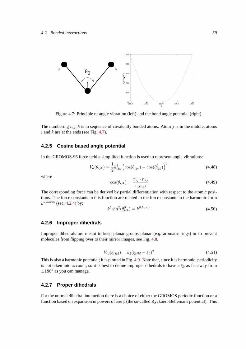
4.2. Bonded interactions 59
θ0
100.0�
110.0�
120.0�
130.0�
140.0�
θ
0.0
10.0
20.0
30.0
40.0
50.0
Va
(kJ
mol
e
�
–1)
Figure 4.7: Principle of angle vibration (left) and the bond angle potential (right).
The numberingi, j, k is in sequence of covalently bonded atoms. Atomj is in the middle; atomsi andk are at the ends (see Fig.4.7).
4.2.5 Cosine based angle potential
In the GROMOS-96 force field a simplified function is used to represent angle vibrations:
Va(θijk) =12kθ
ijk
(cos(θijk)− cos(θ0
ijk))2
(4.48)
wherecos(θijk) =
rij · rkj
rijrkj(4.49)
The corresponding force can be derived by partial differentiation with respect to the atomic posi-tions. The force constants in this function are related to the force constants in the harmonic formkθ,harm (sec.4.2.4) by:
kθ sin2(θ0ijk) = kθ,harm (4.50)
4.2.6 Improper dihedrals
Improper dihedrals are meant to keep planar groups planar (e.g. aromatic rings) or to preventmolecules from flipping over to their mirror images, see Fig.4.8.
Vid(ξijkl) = kξ(ξijkl − ξ0)2 (4.51)
This is also a harmonic potential; it is plotted in Fig.4.9. Note that, since it is harmonic, periodicityis not taken into account, so it is best to define improper dihedrals to have aξ0 as far away from±180◦ as you can manage.
4.2.7 Proper dihedrals
For the normal dihedral interaction there is a choice of either the GROMOS periodic function or afunction based on expansion in powers ofcosφ (the so-called Ryckaert-Bellemans potential). This

60 Chapter 4. Force fields
k
li
j
i
kj
l
k
i
j
l
Figure 4.8: Principle of improper dihedral angles. Out of plane bending for rings (left), sub-stituents of rings (middle), out of tetrahedral (right). The improper dihedral angleξ is defined asthe angle between planes (i,j,k) and (j,k,l) in all cases.
–20.0 –10.0 0.0 10.0�
20.0�
ξ
0.0
10.0
20.0
30.0
Vi (
kJ m
ole
�
–1)
Figure 4.9: Improper dihedral potential.
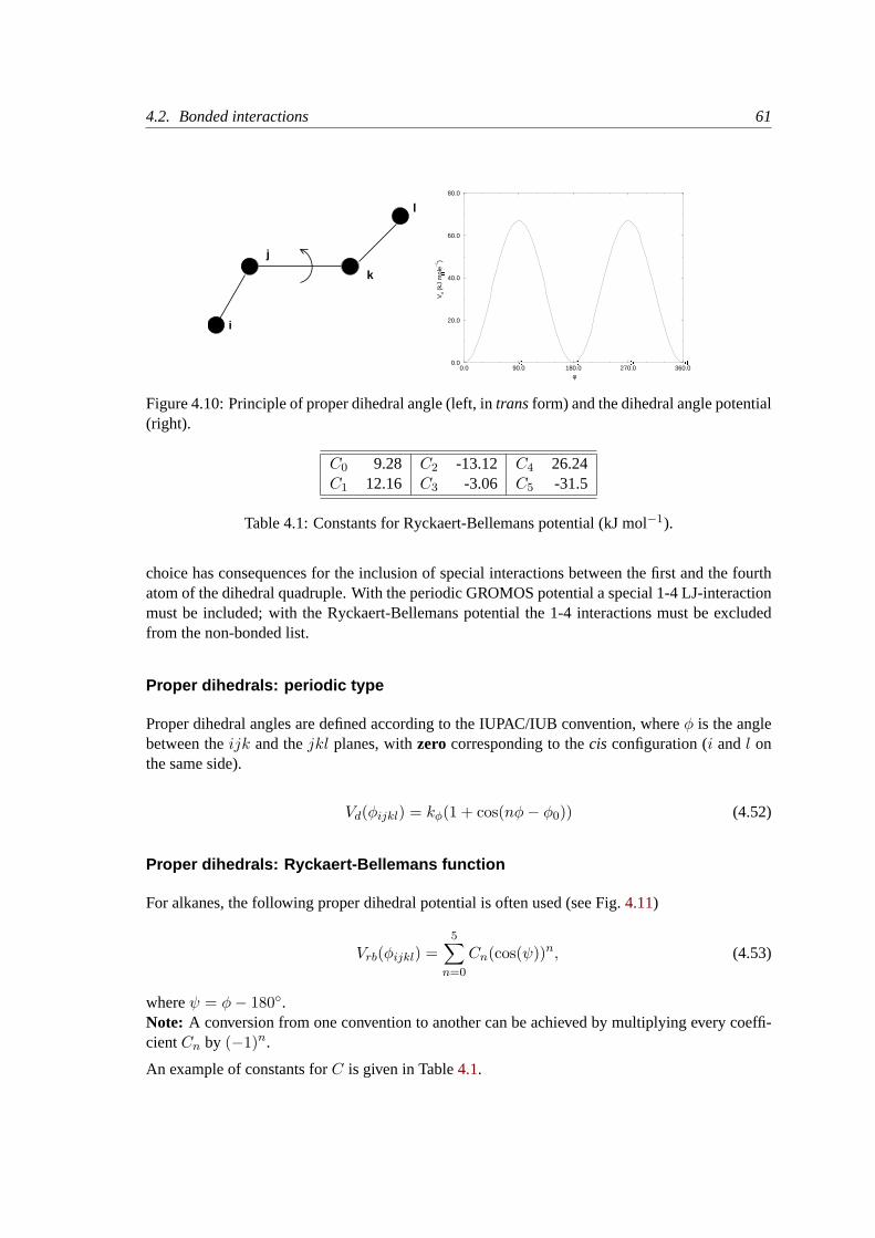
4.2. Bonded interactions 61
j
k
l
i
0.0 90.0�
180.0�
270.0�
360.0�
φ
0.0
20.0
40.0
60.0
80.0
Vd
(kJ
mol
e
�
–1)
Figure 4.10: Principle of proper dihedral angle (left, intransform) and the dihedral angle potential(right).
C0 9.28 C2 -13.12 C4 26.24C1 12.16 C3 -3.06 C5 -31.5
Table 4.1: Constants for Ryckaert-Bellemans potential (kJ mol−1).
choice has consequences for the inclusion of special interactions between the first and the fourthatom of the dihedral quadruple. With the periodic GROMOS potential a special 1-4 LJ-interactionmust be included; with the Ryckaert-Bellemans potential the 1-4 interactions must be excludedfrom the non-bonded list.
Proper dihedrals: periodic type
Proper dihedral angles are defined according to the IUPAC/IUB convention, whereφ is the anglebetween theijk and thejkl planes, withzero corresponding to thecis configuration (i andl onthe same side).
Vd(φijkl) = kφ(1 + cos(nφ− φ0)) (4.52)
Proper dihedrals: Ryckaert-Bellemans function
For alkanes, the following proper dihedral potential is often used (see Fig.4.11)
Vrb(φijkl) =5∑
n=0
Cn(cos(ψ))n, (4.53)
whereψ = φ− 180◦.Note: A conversion from one convention to another can be achieved by multiplying every coeffi-cientCn by (−1)n.
An example of constants forC is given in Table4.1.
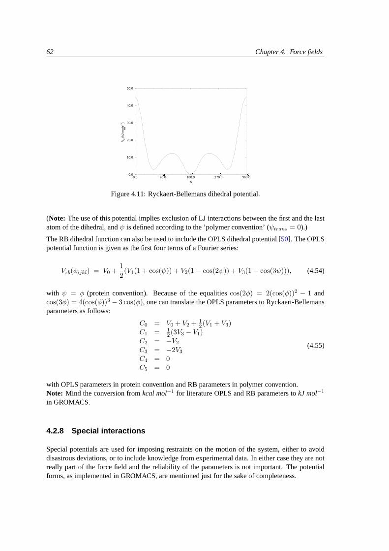
62 Chapter 4. Force fields
0.0 90.0�
180.0�
270.0�
360.0�
φ
0.0
10.0
20.0
30.0
40.0
50.0
Vd
(kJ
mol
e
�
–1)
Figure 4.11: Ryckaert-Bellemans dihedral potential.
(Note: The use of this potential implies exclusion of LJ interactions between the first and the lastatom of the dihedral, andψ is defined according to the ’polymer convention’ (ψtrans = 0).)
The RB dihedral function can also be used to include the OPLS dihedral potential [50]. The OPLSpotential function is given as the first four terms of a Fourier series:
Vrb(φijkl) = V0 +12(V1(1 + cos(ψ)) + V2(1− cos(2ψ)) + V3(1 + cos(3ψ))), (4.54)
with ψ = φ (protein convention). Because of the equalitiescos(2φ) = 2(cos(φ))2 − 1 andcos(3φ) = 4(cos(φ))3 − 3 cos(φ), one can translate the OPLS parameters to Ryckaert-Bellemansparameters as follows:
C0 = V0 + V2 + 12(V1 + V3)
C1 = 12(3V3 − V1)
C2 = −V2
C3 = −2V3
C4 = 0C5 = 0
(4.55)
with OPLS parameters in protein convention and RB parameters in polymer convention.Note: Mind the conversion fromkcal mol−1 for literature OPLS and RB parameters tokJ mol−1
in GROMACS.
4.2.8 Special interactions
Special potentials are used for imposing restraints on the motion of the system, either to avoiddisastrous deviations, or to include knowledge from experimental data. In either case they are notreally part of the force field and the reliability of the parameters is not important. The potentialforms, as implemented in GROMACS, are mentioned just for the sake of completeness.
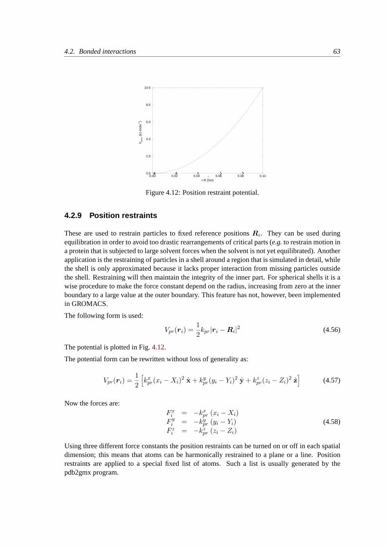
4.2. Bonded interactions 63
0.00�
0.02�
0.04�
0.06�
0.08�
0.10�
r-R (nm)�
0.0
2.0
4.0
6.0
8.0
10.0
Vpo
sre
(kJ
mol
e–1)
Figure 4.12: Position restraint potential.
4.2.9 Position restraints
These are used to restrain particles to fixed reference positionsRi. They can be used duringequilibration in order to avoid too drastic rearrangements of critical parts (e.g.to restrain motion ina protein that is subjected to large solvent forces when the solvent is not yet equilibrated). Anotherapplication is the restraining of particles in a shell around a region that is simulated in detail, whilethe shell is only approximated because it lacks proper interaction from missing particles outsidethe shell. Restraining will then maintain the integrity of the inner part. For spherical shells it is awise procedure to make the force constant depend on the radius, increasing from zero at the innerboundary to a large value at the outer boundary. This feature has not, however, been implementedin GROMACS.
The following form is used:
Vpr(ri) =12kpr|ri −Ri|2 (4.56)
The potential is plotted in Fig.4.12.
The potential form can be rewritten without loss of generality as:
Vpr(ri) =12
[kx
pr(xi −Xi)2 x + kypr(yi − Yi)2 y + kz
pr(zi − Zi)2 z]
(4.57)
Now the forces are:F x
i = −kxpr (xi −Xi)
F yi = −ky
pr (yi − Yi)F z
i = −kzpr (zi − Zi)
(4.58)
Using three different force constants the position restraints can be turned on or off in each spatialdimension; this means that atoms can be harmonically restrained to a plane or a line. Positionrestraints are applied to a special fixed list of atoms. Such a list is usually generated by thepdb2gmx program.
64 Chapter 4. Force fields
4.2.10 Angle restraints
These are used to restrain the angle between two pairs of particles or between one pair of particlesand the Z-axis. The functional form is similar to that of a proper dihedral. For two pairs of atoms:
Var(ri, rj , rk, rl) = kar(1− cos(n(θ − θ0))), where θ = arccos
(rj − ri
‖rj − ri‖· rl − rk
‖rl − rk‖
)(4.59)
For one pair of atoms and the Z-axis:
Var(ri, rj) = kar(1− cos(n(θ − θ0))), where θ = arccos
rj − ri
‖rj − ri‖·
001
(4.60)
A multiplicity (n) of 2 is useful when you do not want to distinguish between parallel and anti-parallel vectors.
4.2.11 Distance restraints
Distance restraints add a penalty to the potential when the distance between specified pairs ofatoms exceeds a threshold value. They are normally used to impose experimental restraints, asfrom experiments in nuclear magnetic resonance (NMR), on the motion of the system. Thus MDcan be used for structure refinement using NMR data. If one just wants to the restrain the distancebetween two particles using a harmonic potential one should use[ bonds ] type 6 (see5.3.5).The potential form for distance restraints is quadratic below a specified lower bound and betweentwo specified upper bounds and linear beyond the largest bound (see Fig.4.13).
Vdr(rij) =
12kdr(rij − r0)2 for rij < r0
0 for r0 ≤ rij < r1
12kdr(rij − r1)2 for r1 ≤ rij < r2
12kdr(r2 − r1)(2rij − r2 − r1) for r2 ≤ rij
(4.61)
The forces are
F i =
−kdr(rij − r0)rij
rijfor rij < r0
0 for r0 ≤ rij < r1
−kdr(rij − r1)rij
rijfor r1 ≤ rij < r2
−kdr(r2 − r1)rij
rijfor r2 ≤ rij
(4.62)
Time averaging
Distance restraints based on instantaneous distances can potentially reduce the fluctuations in amolecule significantly. This problem can be overcome by restraining to atime averageddis-
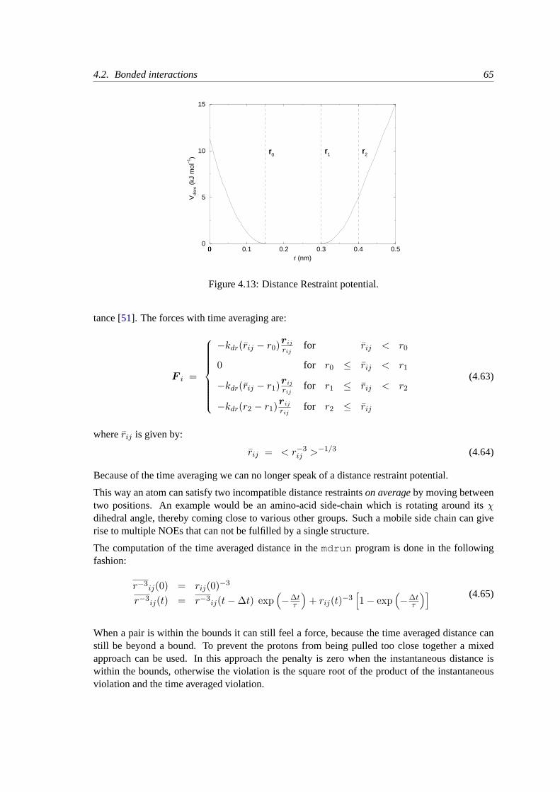
4.2. Bonded interactions 65
0�
0.1 0.2 0.3 0.4 0.5r (nm)
0
5
10
15
Vdi
sre
(kJ
mol
−1 )
r0 r1 r2
Figure 4.13: Distance Restraint potential.
tance [51]. The forces with time averaging are:
F i =
−kdr(rij − r0)rij
rijfor rij < r0
0 for r0 ≤ rij < r1
−kdr(rij − r1)rij
rijfor r1 ≤ rij < r2
−kdr(r2 − r1)rij
rijfor r2 ≤ rij
(4.63)
whererij is given by:
rij = < r−3ij >−1/3 (4.64)
Because of the time averaging we can no longer speak of a distance restraint potential.
This way an atom can satisfy two incompatible distance restraintson averageby moving betweentwo positions. An example would be an amino-acid side-chain which is rotating around itsχdihedral angle, thereby coming close to various other groups. Such a mobile side chain can giverise to multiple NOEs that can not be fulfilled by a single structure.
The computation of the time averaged distance in themdrun program is done in the followingfashion:
r−3ij(0) = rij(0)−3
r−3ij(t) = r−3
ij(t−∆t) exp(−∆t
τ
)+ rij(t)−3
[1− exp
(−∆t
τ
)] (4.65)
When a pair is within the bounds it can still feel a force, because the time averaged distance canstill be beyond a bound. To prevent the protons from being pulled too close together a mixedapproach can be used. In this approach the penalty is zero when the instantaneous distance iswithin the bounds, otherwise the violation is the square root of the product of the instantaneousviolation and the time averaged violation.
66 Chapter 4. Force fields
Averaging over multiple pairs
Sometimes it is unclear from experimental data which atom pair gives rise to a single NOE, inother occasions it can be obvious that more than one pair contributes due to the symmetry of thesystem,e.g.a methyl group with three protons. For such a group it is not possible to distinguishbetween the protons, therefore they should all be taken into account when calculating the distancebetween this methyl group and another proton (or group of protons). Due to the physical nature ofmagnetic resonance, the intensity of the NOE signal is inversely proportional to the sixth powerof the interatomic distance. Thus, when combining atom pairs, a fixed list ofN restraints may betaken together, where the apparent “distance” is given by:
rN (t) =
[N∑
n=1
rn(t)−6
]−1/6
(4.66)
where we userij or eqn.4.64for thern. TherN of the instantaneous and time-averaged distancescan be combined to do a mixed restraining as indicated above. As more pairs of protons contributeto the same NOE signal, the intensity will increase, and the summed “distance” will be shorterthan any of its components due to the reciprocal summation.
There are two options for distributing the forces over the atom pairs. In the conservative optionthe force is defined as the derivative of the restraint potential with respect to the coordinates. Thisresults in a conservative potential when time averaging is not used. The force distribution over thepairs is proportional tor−6. This means that a close pair feels a much larger force than a distantpair, which might lead to a ’too rigid’ molecule. The other option is an equal force distribution.In this case each pair feels1/N of the derivative of the restraint potential with respect torN . Theadvantage of this method is that more conformations might be sampled, but the non-conservativenature of the forces can lead to local heating of the protons.
It is also possible to useensemble averagingusing multiple (protein) molecules. In this case thebounds should be lowered as in:
r1 = r1 ∗M−1/6
r2 = r2 ∗M−1/6 (4.67)
whereM is the number of molecules. The GROMACS preprocessorgrompp can do this auto-matically when the appropriate option is given. The resulting “distance” is then used to calculatethe scalar force according to:
F i = 0 rN < r1= − kdr(rN − r1)
rij
rijr1 ≤ rN < r2
= − kdr(r2 − r1)rij
rijrN ≥ r2
(4.68)
wherei andj denote the atoms of all the pairs that contribute to the NOE signal.
Using distance restraints
A list of distance restrains based on NOE data can be added to a molecule definition in yourtopology file, like in the following example:
4.2. Bonded interactions 67
[ distance_restraints ]; ai aj type index type’ low up1 up2 fac10 16 1 0 1 0.0 0.3 0.4 1.010 28 1 1 1 0.0 0.3 0.4 1.010 46 1 1 1 0.0 0.3 0.4 1.016 22 1 2 1 0.0 0.3 0.4 2.516 34 1 3 1 0.0 0.5 0.6 1.0
In this example a number of features can be found. In columnsai andaj you find the atomnumbers of the particles to be restrained. Thetype column should always be 1. As explainedin sec.4.2.11, multiple distances can contribute to a single NOE signal. In the topology this canbe set using theindex column. In our example, the restraints 10-28 and 10-46 both have index1, therefore they are treated simultaneously. An extra requirement for treating restraints together,is that the restraints should be on successive lines, without any other intervening restraint. Thetype’ column will usually be 1, but can be set to 2 to obtain a distance restraint which will neverbe time and ensemble averaged; this can be useful for restraining hydrogen bonds. The columnslow , up1 andup2 hold the values ofr0, r1 andr2 from eqn.4.61. In some cases it can be usefulto have different force constants for some restraints; this is controlled by the columnfac . Theforce constant in the parameter file is multiplied by the value in the columnfac for each restraint.
Some parameters for NMR refinement can be specified in thegrompp.mdp file:
disre : type of distance restraining. The disre variable sets the type of distance restraint.no/simple turns the distance restraints off/on. When multiple proteins or peptides arepresent in one simulation box, ensemble averaging can be turned on by settingdisre =ensemble . Normally one would perform ensemble averaging over multiple subsystems,each in a separate box, usingmdrun -multi ; supplytopol0.tpr , topol1.tpr , ...with different coordiates and/or velocities.
disre weighting : force-weighting in restraints with multiple pairs. By default, the forcedue to the distance restraint is distributed equally over all the pairs involved in the restraint.This can also be explicitly selected withdisre weighting = equal . If you insteadset this option todisre weighting = conservative you get conservative forceswhendisre tau = 0 .
disre mixed : how to calculate the violations. disre mixed = no gives normal time-averagedviolations. Whendisre mixed = yes the square root of the product of the time-averaged and the instantaneous violations is used.
disre fc : force constantkdr for distance restraints. kdr (eqn. 4.61) can be set as variabledisre fc = 1000 for a force constant of 1000 kJ mol−1 nm−2. This value is multi-plied by the value in thefac column in the distance restraint entries in the topology file.
disre tau : time constant for restraints. τ (eqn.4.65) can be set as variabledisre tau =10 for a time constant of 10 ps. Time averaging can be turned off by settingdisre tauto 0.
nstdisreout : pair distance output frequency. Determines how often the time-averaged andinstantaneous distances of all atom pairs involved in distance restraints are written to theenergy file.
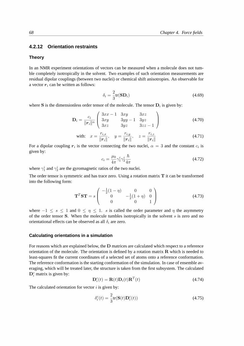
68 Chapter 4. Force fields
4.2.12 Orientation restraints
Theory
In an NMR experiment orientations of vectors can be measured when a molecule does not tum-ble completely isotropically in the solvent. Two examples of such orientation measurements areresidual dipolar couplings (between two nuclei) or chemical shift anisotropies. An observable fora vectorri can be written as follows:
δi =23
tr(SDi) (4.69)
whereS is the dimensionless order tensor of the molecule. The tensorDi is given by:
Di =ci
‖ri‖α
3xx− 1 3xy 3xz3xy 3yy − 1 3yz3xz 3yz 3zz − 1
(4.70)
with: x =ri,x‖ri‖
, y =ri,y‖ri‖
, z =ri,z‖ri‖
(4.71)
For a dipolar couplingri is the vector connecting the two nuclei,α = 3 and the constantci isgiven by:
ci =µ0
4πγi
1γi2
h
4π(4.72)
whereγi1 andγi
2 are the gyromagnetic ratios of the two nuclei.
The order tensor is symmetric and has trace zero. Using a rotation matrixT it can be transformedinto the following form:
TTST = s
−12(1− η) 0 0
0 −12(1 + η) 0
0 0 1
(4.73)
where−1 ≤ s ≤ 1 and 0 ≤ η ≤ 1. s is called the order parameter andη the asymmetryof the order tensorS. When the molecule tumbles isotropically in the solvents is zero and noorientational effects can be observed as allδi are zero.
Calculating orientations in a simulation
For reasons which are explained below, theD matrices are calculated which respect to a referenceorientation of the molecule. The orientation is defined by a rotation matrixR which is needed toleast-squares fit the current coordinates of a selected set of atoms onto a reference conformation.The reference conformation is the starting conformation of the simulation. In case of ensemble av-eraging, which will be treated later, the structure is taken from the first subsystem. The calculatedDc
i matrix is given by:Dc
i (t) = R(t)Di(t)RT (t) (4.74)
The calculated orientation for vectori is given by:
δci (t) =
23
tr(S(t)Dci (t)) (4.75)
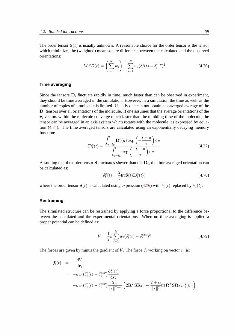
4.2. Bonded interactions 69
The order tensorS(t) is usually unknown. A reasonable choice for the order tensor is the tensorwhich minimizes the (weighted) mean square difference between the calculated and the observedorientations:
MSD(t) =
(N∑
i=1
wi
)−1 N∑i=1
wi(δci (t)− δexp
i )2 (4.76)
Time averaging
Since the tensorsDi fluctuate rapidly in time, much faster than can be observed in experiment,they should be time averaged in the simulation. However, in a simulation the time as well as thenumber of copies of a molecule is limited. Usually one can not obtain a converged average of theDi tensors over all orientations of the molecule. If one assumes that the average orientations of theri vectors within the molecule converge much faster than the tumbling time of the molecule, thetensor can be averaged in an axis system which rotates with the molecule, as expressed by equa-tion (4.74). The time averaged tensors are calculated using an exponentially decaying memoryfunction:
Dai (t) =
∫ t
u=t0Dc
i (u) exp(− t− u
τ
)du∫ t
u=t0exp
(− t− u
τ
)du
(4.77)
Assuming that the order tensorS fluctuates slower than theDi, the time averaged orientation canbe calculated as:
δai (t) =
23
tr(S(t)Dai (t)) (4.78)
where the order tensorS(t) is calculated using expression (4.76) with δci (t) replaced byδa
i (t).
Restraining
The simulated structure can be restrained by applying a force proportional to the difference be-tween the calculated and the experimental orientations. When no time averaging is applied aproper potential can be defined as:
V =12k
N∑i=1
wi(δci (t)− δexp
i )2 (4.79)
The forces are given by minus the gradient ofV . The forcefi working on vectorri is:
fi(t) = −dVdri
= −kwi(δci (t)− δexp
i )dδi(t)dri
= −kwi(δci (t)− δexp
i )2ci
‖r‖2+α
(2RTSRri −
2 + α
‖r‖2tr(RTSRrir
Ti )ri
)
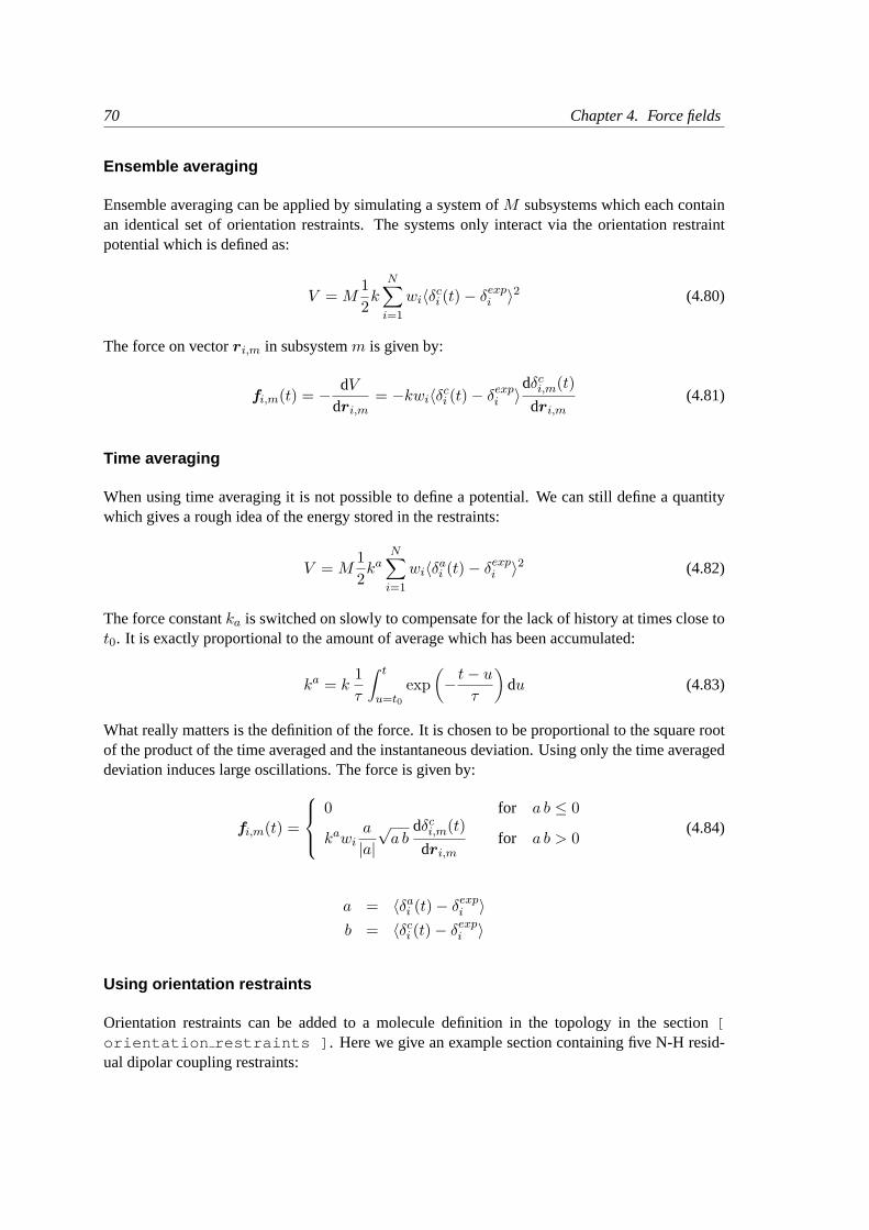
70 Chapter 4. Force fields
Ensemble averaging
Ensemble averaging can be applied by simulating a system ofM subsystems which each containan identical set of orientation restraints. The systems only interact via the orientation restraintpotential which is defined as:
V = M12k
N∑i=1
wi〈δci (t)− δexp
i 〉2 (4.80)
The force on vectorri,m in subsystemm is given by:
fi,m(t) = − dVdri,m
= −kwi〈δci (t)− δexp
i 〉dδc
i,m(t)dri,m
(4.81)
Time averaging
When using time averaging it is not possible to define a potential. We can still define a quantitywhich gives a rough idea of the energy stored in the restraints:
V = M12ka
N∑i=1
wi〈δai (t)− δexp
i 〉2 (4.82)
The force constantka is switched on slowly to compensate for the lack of history at times close tot0. It is exactly proportional to the amount of average which has been accumulated:
ka = k1τ
∫ t
u=t0exp
(− t− u
τ
)du (4.83)
What really matters is the definition of the force. It is chosen to be proportional to the square rootof the product of the time averaged and the instantaneous deviation. Using only the time averageddeviation induces large oscillations. The force is given by:
fi,m(t) =
0 for a b ≤ 0
kawia
|a|√a b
dδci,m(t)
dri,mfor a b > 0
(4.84)
a = 〈δai (t)− δexp
i 〉b = 〈δc
i (t)− δexpi 〉
Using orientation restraints
Orientation restraints can be added to a molecule definition in the topology in the section[orientation restraints ] . Here we give an example section containing five N-H resid-ual dipolar coupling restraints:
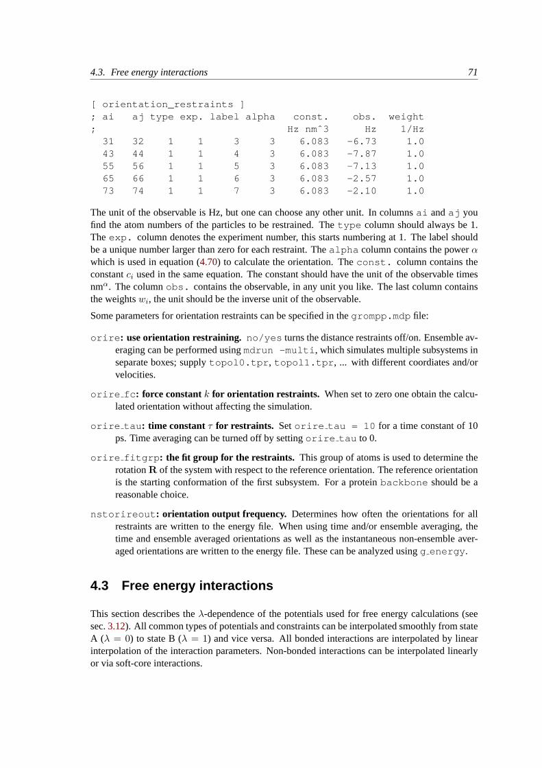
4.3. Free energy interactions 71
[ orientation_restraints ]; ai aj type exp. label alpha const. obs. weight; Hz nmˆ3 Hz 1/Hz
31 32 1 1 3 3 6.083 -6.73 1.043 44 1 1 4 3 6.083 -7.87 1.055 56 1 1 5 3 6.083 -7.13 1.065 66 1 1 6 3 6.083 -2.57 1.073 74 1 1 7 3 6.083 -2.10 1.0
The unit of the observable is Hz, but one can choose any other unit. In columnsai andaj youfind the atom numbers of the particles to be restrained. Thetype column should always be 1.Theexp. column denotes the experiment number, this starts numbering at 1. The label shouldbe a unique number larger than zero for each restraint. Thealpha column contains the powerαwhich is used in equation (4.70) to calculate the orientation. Theconst. column contains theconstantci used in the same equation. The constant should have the unit of the observable timesnmα. The columnobs. contains the observable, in any unit you like. The last column containsthe weightswi, the unit should be the inverse unit of the observable.
Some parameters for orientation restraints can be specified in thegrompp.mdp file:
orire : use orientation restraining. no/yes turns the distance restraints off/on. Ensemble av-eraging can be performed usingmdrun -multi , which simulates multiple subsystems inseparate boxes; supplytopol0.tpr , topol1.tpr , ... with different coordiates and/orvelocities.
orire fc : force constantk for orientation restraints. When set to zero one obtain the calcu-lated orientation without affecting the simulation.
orire tau : time constant τ for restraints. Setorire tau = 10 for a time constant of 10ps. Time averaging can be turned off by settingorire tau to 0.
orire fitgrp : the fit group for the restraints. This group of atoms is used to determine therotationR of the system with respect to the reference orientation. The reference orientationis the starting conformation of the first subsystem. For a proteinbackbone should be areasonable choice.
nstorireout : orientation output frequency. Determines how often the orientations for allrestraints are written to the energy file. When using time and/or ensemble averaging, thetime and ensemble averaged orientations as well as the instantaneous non-ensemble aver-aged orientations are written to the energy file. These can be analyzed usingg energy .
4.3 Free energy interactions
This section describes theλ-dependence of the potentials used for free energy calculations (seesec.3.12). All common types of potentials and constraints can be interpolated smoothly from stateA (λ = 0) to state B (λ = 1) and vice versa. All bonded interactions are interpolated by linearinterpolation of the interaction parameters. Non-bonded interactions can be interpolated linearlyor via soft-core interactions.
72 Chapter 4. Force fields
Harmonic potentials
The example given here is for the bond potential, which is harmonic in GROMACS. However,these equations apply to the angle potential and the improper dihedral potential as well.
Vb =12((1− λ)kA
b + λkBb )(b− (1− λ)bA0 − λbB0 )2 (4.85)
∂Vb
∂λ=
12(kB
b − kAb )[b− (1− λ)bA0 + λbB0 )2 + (bA0 − bB0 )(b− (1− λ)bA0 − λbB0 )
](4.86)
GROMOS-96 bonds and angles
Fourth power bond stretching and cosine based angle potentials are interpolated by linear interpo-lation of the force constant and the equilibrium position. Formulas are not given here.
Proper dihedrals
For the proper dihedrals, the equations are somewhat more complicated:
Vd = ((1− λ)kAd + λkB
d )(1 + cos(nφφ− ((1− λ)φA0 + λφB
0 )) (4.87)∂Vd
∂λ= (kB
d − kAd )[1 + cos(nφφ− [(1− λ)φA
0 + λφB0 ])−
((1− λ)kAd + λkB
d )(φA0 − φB
0 ) sin(nφφ− [(1− λ)φA0 + λφB
0 ]]
(4.88)
Note: that the multiplicitynφ can not be parameterized because the function should remain peri-odic on the interval[0, 2π].
Coulomb interaction
The Coulomb interaction between two particles of which the charge varies withλ is:
Vc =f
εrfrij
[((1− λ)qA
i + λqBi ) · ((1− λ)qA
j + λqBi )]
(4.89)
∂Vc
∂λ=
f
εrfrij
[(qB
j − qAj )((1− λ)qA
i + λqBi ) + (qB
i − qAi )((1− λ)qA
j + λqBj )](4.90)
wheref = 14πε0
= 138.935 485 (see chapter2)
Coulomb interaction with Reaction Field
The coulomb interaction including a reaction field, between two particles of which the chargevaries withλ is:
Vc = f
[1rij
+ krf r2ij − crf
] [((1− λ)qA
i + λqBi ) · ((1− λ)qA
j + λqBi )]
(4.91)
4.3. Free energy interactions 73
∂Vc
∂λ= f
[1rij
+ krf r2ij − crf
]·[
(qBj − qA
j )((1− λ)qAi + λqB
i ) + (qBi − qA
i )((1− λ)qAj + λqB
j )]
(4.92)
Note that the constantskrf andcrf are defined using the dielectric constantεrf of the medium(see sec.4.1.4).
Lennard-Jones interaction
For the Lennard-Jones interaction between two particles of which theatom typevaries withλ wecan write:
VLJ =((1− λ)CA
12 + λCB12)
r12ij
− (1− λ)CA6 + λCB
6
r6ij(4.93)
∂VLJ
∂λ=
CB12 − CA
12
r12ij
− CB6 − CA
6
r6ij(4.94)
It should be noted that it is also possible to express a pathway from state A to state B usingσ andε (see eqn.4.5). It may seem to make sense physically, to vary the forcefield parametersσ andεrather than the derived parametersC12 andC6. However, the difference between the pathways inparameter space is not large, and the free energy itself does not depend on the pathway, so we usethe simple formulation presented above.
Kinetic Energy
When the mass of a particle changes, there is also a contribution of the kinetic energy to the freeenergy (note that we can not write the momentump as mv, since that would result in the sign of∂Ek∂λ being incorrect [52]):
Ek =12
p2
(1− λ)mA + λmB(4.95)
∂Ek
∂λ= −1
2p2(mB −mA)
((1− λ)mA + λmB)2(4.96)
after taking the derivative, wecan insertp = mv, such that:
∂Ek
∂λ= − 1
2v2(mB −mA) (4.97)
Constraints
The constraints are formally part of the Hamiltonian, and therefore they give a contribution to thefree energy. In GROMACS this can be calculated using the LINCS or the SHAKE algorithm. Ifwe have a number of constraint equationsgk:
gk = rk − dk (4.98)

74 Chapter 4. Force fields
0�
0.5 1� 1.5 2�
2.5 3�
r�
−1
0
1
2
3
4
5
Vsc�
LJ, α=0LJ, α=1.5LJ, α=23/r,
�α=0
3/r, �
α=1.53/r,
�α=2
Figure 4.14: Soft-core interactions atλ = 0.5, with CA6 = CA
12 = CB6 = CB
12 = 1.
whererk is the distance vector between two particles anddk is the constraint distance betweenthe two particles, we can write this using aλ-dependent distance as
gk = rk −((1− λ)dA
k + λdBk
)(4.99)
the contributionCλ to the Hamiltonian using Lagrange multipliersλ:
Cλ =∑k
λkgk (4.100)
∂Cλ
∂λ=
∑k
λk
(dB
k − dAk
)(4.101)
4.3.1 Soft-core interactions
The linear interpolation of the Lennard-Jones and Coulomb potentials gives problems when grow-ing particles out of nothing or when making particles disappear (λ close to 0 or 1). To circumventthese problems, the singularities in the potentials need to be removed. This is done with soft-corepotentials. In GROMACS the soft-core potentialVsc is:
Vsc(r) = (1− λ)V A(rA) + λV B(rB) (4.102)
rA =(ασ6
Aλ2 + r6
) 16 (4.103)
rB =(ασ6
B(1− λ)2 + r6) 1
6 (4.104)
whereV A andV B are the normal “hard core” Van der Waals or electrostatic potentials in state A(λ = 0) and state B (λ = 1) respectively,α is the soft-core parameter, which mainly controls theheight of the potential aroundr = 0, σ is the radius of the interaction, which is(C12/C6)1/6 ora predefined value whenC6 or C12 is zero. For intermediateλ, rA andrB alter the interactions

4.4. Methods 75
i+1 i+3
i i+2 i+4
Figure 4.15: Atoms along an alkane chain.
very little whenr > α1/6σ and they quickly switch the soft-core interaction to an almost constantvalue whenr becomes smaller (Fig.4.14). The force is:
Fsc(r) = −∂Vsc(r)∂r
= (1− λ)FA(rA)(r
rA
)5
+ λFB(rB)(r
rB
)5
(4.105)
whereFA andFB are the ’hard core’ forces. The contribution to the derivative of the free energyis:
∂Vsc(r)∂λ
= −V A(rA) + V B(rB) +13αλ(1− λ)
(−FA(rA)σ6
Ar−5A + FB(rB)σ6
Br−5B
)(4.106)
4.4 Methods
4.4.1 Exclusions and 1-4 Interactions.
Atoms within a molecule that are close by in the chain,i.e. atoms that are covalently bonded, orlinked by one respectively two atoms are so-calledfirst neighbors, second neighborsand thirdneighbors, (see Fig.4.15). Since the interactions of atomi with atomsi+1 andi+2
are mainly quantum mechanical, they can not be modeled by a Lennard-Jones potential. Instead itis assumed that these interactions are adequately modeled by a harmonic bond term or constraint(i, i+1) and a harmonic angle term (i, i+2). The first and second neighbors (atomsi+1 andi+2) arethereforeexcludedfrom the Lennard-Jones interaction list of atomi; atomsi+1 andi+2 are calledexclusionsof atomi.
For third neighbors the normal Lennard-Jones repulsion is sometimes still too strong, which meansthat when applied to a molecule the molecule would deform or break due to the internal strain.This is especially the case for carbon-carbon interactions in acis-conformation (e.g. cis-butane).Therefore for some of these interactions the Lennard-Jones repulsion has been reduced in theGROMOS force field, which is implemented by keeping a separate list of 1-4 and normal Lennard-Jones parameters. In other force fields, such as OPLS [50], the standard Lennard-Jones parametersare reduced by a factor of two, but in that case also the dispersion (r−6) and the coulomb interactionare scaled. GROMACS can use either of these methods.
4.4.2 Charge Groups.
In principle the force calculation in MD is anO(N2) problem. Therefore we apply a cutoff fornon-bonded force (NBF) calculations: only the particles within a certain distance of each other
76 Chapter 4. Force fields
are interacting. This reduces the cost toO(N) (typically 100N to 200N ) of the NBF. It alsointroduces an error, which is, in most cases, acceptable, except when applying the cutoff impliesthe creation of charges, in which case you should consider using the lattice sum methods providedby GROMACS.
Consider a water molecule interacting with another atom. When we would apply the cutoff on anatom-atom basis we might include the atom-Oxygen interaction (with a charge of -0.82) withoutthe compensating charge of the protons and so induce a large dipole moment over the system.Therefore we have to keep groups of atoms with total charge 0 together. These groups are calledcharge groups.
4.4.3 Treatment of cutoffs
GROMACS is quite flexible in treating cutoffs, which implies there can be quite a number ofparameters to set. These parameters are set in the input file for grompp. There are two sort ofparameters that affect the cutoff interactions; you can select which type of interaction to use ineach case, and which cutoffs should be used in the neighborsearching.
For both Coulomb and van der Waals interactions there are interaction type selectors (termedvdwtype and coulombtype ) and two parameters, for a total of six nonbonded interactionparameters. See sec.7.3.1for a complete description of these parameters.
The neighbor searching (NS) can be performed using a single-range, or a twin-range approach.Since the former is merely a special case of the latter we will discuss the more general twin-range.In this case NS is described by two radiirlist and max(rcoulomb ,rvdw ). Usually one buildsthe neighbor list every 10 time steps or every 20 fs (parameternstlist ). In the neighbor list allinteraction pairs that fall withinrlist are stored. Furthermore, the interactions between pairsthat do not fall withinrlist but do fall within max(rcoulomb ,rvdw ) are computed duringNS, and the forces and energy are stored separately, and added to short-range forces at every timestep between successive NS. Ifrlist = max(rcoulomb ,rvdw ), no forces are evaluated duringneighbor list generation. The virial is calculated from the sum of the short- and long-range forces.This means that the virial can be slightly asymmetrical at non-NS steps. In single precision thevirial is almost always asymmetrical, because the off-diagonal elements are about as large as eachelement in the sum. In most cases this is not really a problem, since the fluctuations in de virialcan be 2 orders of magnitude larger than the average.
Except for the plain cutoff, all of the interaction functions in Table4.2 require that neighborsearching is done with a larger radius than therc specified for the functional form, because of theuse of charge groups. The extra radius is typically of the order of 0.25 nm (roughly the largestdistance between two atoms in a charge group plus the distance a charge group can diffuse withinneighbor list updates).
4.5 Dummy atoms.
Dummy atoms can be used in GROMACS in a number of ways. We write the position of thedummy particlerd as a function of the positions of other particlesri: rd = f(r1..rn). Thedummy, which may carry charge, or can be involved in other interactions can now be used in the
4.5. Dummy atoms. 77
Type ParametersCoulomb Plain cutoff rc, εr
Reaction field rc, εrf
Shift function r1, rc, εrSwitch function r1, rc, εr
VdW Plain cutoff rcShift function r1, rcSwitch function r1, rc
Table 4.2: Parameters for the different functional forms of the non-bonded interactions.
force calculation. The force acting on the dummy particle must be redistributed over the atomsin a consistent way. A good way to do this can be found in ref. [53]. We can write the potentialenergy as
V = V (rd, r1..rn) = V ∗(r1..rn) (4.107)
The force on the particlei is then
F i = −∂V∗
∂ri= −∂V
∂ri− ∂rd
∂ri
∂V
∂rd= F direct
i + F ′i (4.108)
the first term of which is the normal force. The second term is the force on particlei due to thedummy particle, which can be written in tensor notation:
F ′i =
∂xd
∂xi
∂yd
∂xi
∂zd∂xi
∂xd
∂yi
∂yd
∂yi
∂zd∂yi
∂xd
∂zi
∂yd
∂zi
∂zd∂zi
F d (4.109)
whereF d is the force on the dummy particle andxd, yd andzd are the coordinates of the dummyparticle. In this way the total force and the total torque are conserved [53].
As a further note, the computation of the virial (eqn.3.18) is non-trivial when dummy atoms areused. Since the virial involves a summation over all the atoms (rather than virtual particles) theforces most be redistributed from the dummies to the atoms (using eqn.4.109) beforecomputationof the virial. In some special cases where the forces on the atoms can be written as a linearcombination of the forces on the dummies (types 2 and 3 below) there is no difference betweencomputing the virial before and after the redistribution of forces. However, in the general caseredistribution should be done first.
There are six ways to construct dummies from surrounding atoms in GROMACS, which we clas-sify by the number of constructing atoms. Note that all dummy types mentioned can be con-structed from types 3fd (normalized, in-plane) and 3out (non-normalized, out of plane). However,the amount of computation involved increases sharply along this list, so we strongly recommendedusing the first adequate dummy type that will be sufficient for a certain purpose. Fig.4.16givesan overview of the available dummy constructions.
2. As a linear combination of two atoms (Fig.4.162):
rd = ri + arij (4.110)
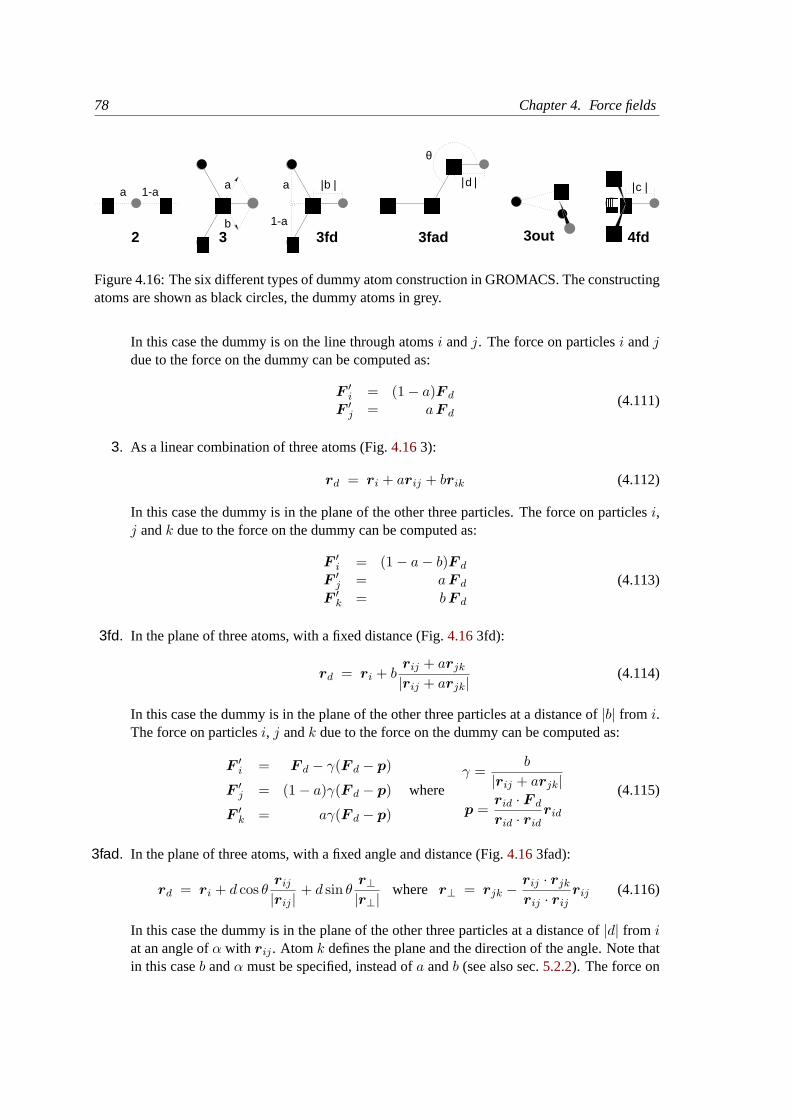
78 Chapter 4. Force fields
������������������������������������ ����������
���������� | |
3fd
| || |1-a
a
b
a
1-a
a������������������������ ���
�������
2 3fad 3out 4fd
cb
3
������������������������
θ
d
� � � � ����������
������������������������
������������������������
�������������������������������
�����������������
�������������������� �����
��������������� �������
�����������������
��������������������
Figure 4.16: The six different types of dummy atom construction in GROMACS. The constructingatoms are shown as black circles, the dummy atoms in grey.
In this case the dummy is on the line through atomsi andj. The force on particlesi andjdue to the force on the dummy can be computed as:
F ′i = (1− a)F d
F ′j = aF d
(4.111)
3. As a linear combination of three atoms (Fig.4.163):
rd = ri + arij + brik (4.112)
In this case the dummy is in the plane of the other three particles. The force on particlesi,j andk due to the force on the dummy can be computed as:
F ′i = (1− a− b)F d
F ′j = aF d
F ′k = bF d
(4.113)
3fd. In the plane of three atoms, with a fixed distance (Fig.4.163fd):
rd = ri + brij + arjk
|rij + arjk|(4.114)
In this case the dummy is in the plane of the other three particles at a distance of|b| from i.The force on particlesi, j andk due to the force on the dummy can be computed as:
F ′i = F d − γ(F d − p)
F ′j = (1− a)γ(F d − p)
F ′k = aγ(F d − p)
whereγ =
b
|rij + arjk|
p =rid · F d
rid · ridrid
(4.115)
3fad. In the plane of three atoms, with a fixed angle and distance (Fig.4.163fad):
rd = ri + d cos θrij
|rij |+ d sin θ
r⊥|r⊥|
where r⊥ = rjk −rij · rjk
rij · rijrij (4.116)
In this case the dummy is in the plane of the other three particles at a distance of|d| from iat an angle ofα with rij . Atom k defines the plane and the direction of the angle. Note thatin this caseb andα must be specified, instead ofa andb (see also sec.5.2.2). The force on
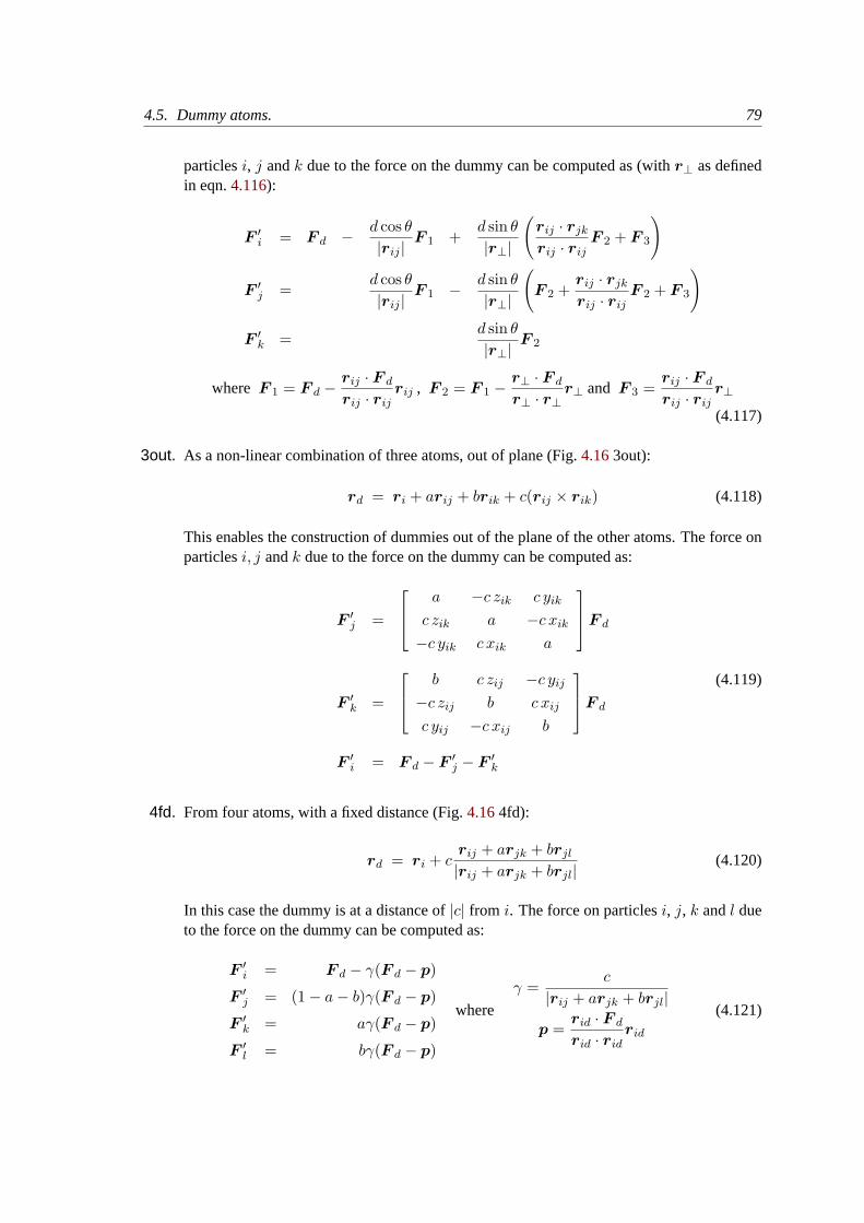
4.5. Dummy atoms. 79
particlesi, j andk due to the force on the dummy can be computed as (withr⊥ as definedin eqn.4.116):
F ′i = F d − d cos θ
|rij |F 1 +
d sin θ|r⊥|
(rij · rjk
rij · rijF 2 + F 3
)
F ′j =
d cos θ|rij |
F 1 − d sin θ|r⊥|
(F 2 +
rij · rjk
rij · rijF 2 + F 3
)
F ′k =
d sin θ|r⊥|
F 2
where F 1 = F d −rij · F d
rij · rijrij , F 2 = F 1 −
r⊥ · F d
r⊥ · r⊥r⊥ and F 3 =
rij · F d
rij · rijr⊥
(4.117)
3out. As a non-linear combination of three atoms, out of plane (Fig.4.163out):
rd = ri + arij + brik + c(rij × rik) (4.118)
This enables the construction of dummies out of the plane of the other atoms. The force onparticlesi, j andk due to the force on the dummy can be computed as:
F ′j =
a −c zik c yik
c zik a −c xik
−c yik c xik a
F d
F ′k =
b c zij −c yij
−c zij b c xij
c yij −c xij b
F d
F ′i = F d − F ′
j − F ′k
(4.119)
4fd. From four atoms, with a fixed distance (Fig.4.164fd):
rd = ri + crij + arjk + brjl
|rij + arjk + brjl|(4.120)
In this case the dummy is at a distance of|c| from i. The force on particlesi, j, k andl dueto the force on the dummy can be computed as:
F ′i = F d − γ(F d − p)
F ′j = (1− a− b)γ(F d − p)
F ′k = aγ(F d − p)
F ′l = bγ(F d − p)
where
γ =c
|rij + arjk + brjl|
p =rid · F d
rid · ridrid
(4.121)
80 Chapter 4. Force fields
4.6 Long Range Electrostatics
4.6.1 Ewald summation
The total electrostatic energy ofN particles and the periodic images are given by
V =f
2
∑nx
∑ny
∑nz∗
N∑i
N∑j
qiqjrij,n
. (4.122)
(nx, ny, nz) = n is the box index vector, and the star indicates that terms withi = j should beomitted when(nx, ny, nz) = (0, 0, 0). The distancerij,n is the real distance between the chargesand not the minimum-image. This sum is conditionally convergent, but very slow.
Ewald summation was first introduced as a method to calculate long-range interactions of the pe-riodic images in crystals [54]. The idea is to convert the single slowly-converging sum eqn.4.122into two quickly-converging terms and a constant term:
V = Vdir + Vrec + V0 (4.123)
Vdir =f
2
N∑i,j
∑nx
∑ny
∑nz∗
qiqjerfc(βrij,n)
rij,n(4.124)
Vrec =f
2πV
N∑i,j
qiqj∑mx
∑my
∑mz∗
exp(−(πm/β)2 + 2πim · (ri − rj)
)m2
(4.125)
V0 = − fβ√π
N∑i
q2i , (4.126)
whereβ is a parameter that determines the relative weight of the direct and reciprocal sums andm = (mx,my,mz). In this way we can use a short cutoff (of the order of1 nm) in the directspace sum and a short cutoff in the reciprocal space sum (e.g.10 wave vectors in each direction).Unfortunately, the computational cost of the reciprocal part of the sum increases asN2 (orN3/2
with a slightly better algorithm) and it is therefore not realistic for use in large systems.
Using Ewald
Don’t use Ewald unless you are absolutely sure this is what you want - for almost all cases the PMEmethod below will perform much better. If you still want to employ classical Ewald summationenter this in your.mdp file, if the side of your box is about3 nm:
coulombtype = Ewaldrvdw = 0.9rlist = 0.9rcoulomb = 0.9fourierspacing = 0.6ewald_rtol = 1e-5

4.6. Long Range Electrostatics 81
The fourierspacing parameter times the box dimensions determines the highest magnitudeof wave vectorsmx,my,mz to use in each direction. With a 3 nm cubic box this example woulduse11 wave vectors (from−5 to 5) in each direction. Theewald rtol parameter is the relativestrength of the electrostatic interaction at the cutoff. Decreasing this gives you a more accuratedirect sum, but a less accurate reciprocal sum.
4.6.2 PME
Particle-mesh Ewald is a method proposed by Tom Darden [55, 56] to improve the performanceof the reciprocal sum. Instead of directly summing wave vectors, the charges are assigned to agrid using cardinal B-spline interpolation. This grid is then Fourier transformed with a 3D FFTalgorithm and the reciprocal energy term obtained by a single sum over the grid in k-space.
The potential at the grid points is calculated by inverse transformation, and by using the interpo-lation factors we get the forces on each atom.
The PME algorithm scales asN log(N), and is substantially faster than ordinary Ewald summa-tion on medium to large systems. On very small systems it might still be better to use Ewald toavoid the overhead in setting up grids and transforms.
Using PME
To use Particle-mesh Ewald summation in GROMACS, specify the following lines in your.mdpfile:
coulombtype = PMErvdw = 0.9rlist = 0.9rcoulomb = 0.9fourierspacing = 0.12pme_order = 4ewald_rtol = 1e-5
In this case thefourierspacing parameter determines the maximum spacing for the FFT gridandpme order controls the interpolation order. Using 4th order (cubic) interpolation and thisspacing should give electrostatic energies accurate to about5 · 10−3. Since the Lennard-Jonesenergies are not this accurate it might even be possible to increase this spacing slightly.
Pressure scaling works with PME, but be aware of the fact that anisotropic scaling can introduceartificial ordering in some systems.
4.6.3 PPPM
The Particle-Particle Particle-Mesh methods of Hockney & Eastwood can also be applied in GRO-MACS for the treatment of long range electrostatic interactions [57, 55, 58]. With this algorithmthe charges of all particles are spread over a grid of dimensions (nx,ny,nz) using a weighting
82 Chapter 4. Force fields
function called the triangle-shaped charged distribution:
W (r) = W (x) W (y) W (z)
W (ξ) =
34 −
(ξh
)2|ξ| ≤ h
2
12
(32 −
|ξ|h
)2h2 < |ξ| < 3h
2
0 3h2 ≤ |ξ|
(4.127)
whereξ (is x, y or z) is the distance to a grid point in the corresponding dimension. Only the 27closest grid points need to be taken into account for each charge.
Then, this charge distribution is Fourier transformed using a 3D inverse FFT routine. In Fourierspace a convolution with functionG is performed:
G(k) =g(k)ε0k2
(4.128)
where g is the Fourier transform of the charge spread function g(r). This yield the long rangepotentialφ(k) on the mesh, which can be transformed using a forward FFT routine into the realspace potential. Finally the potential and forces are retrieved using interpolation [58]. It is not easyto calculate the full long-range virial tensor with PPPM, but it is possible to obtain the trace. Thismeans that the sum of the pressure components is correct (and therefore the isotropic pressure) butnot necessarily the individual pressure components!
Using PPPM
To use the PPPM algorithm in GROMACS, specify the following lines in your.mdp file:
coulombtype = PPPMrlist = 1.0rcoulomb = 0.85rcoulomb_switch = 0.0rvdw = 1.0fourierspacing = 0.075
For details on the switch parameters see the section on modified long-range interactions in thismanual. When using PPPM we recommend to take at most 0.075 nm per gridpoint (e.g.20 grid-points for 1.5 nm). PPPM does not provide the same accuracy as PME but can be slightly fasterin some cases. Due to the problem with the pressure tensor you shouldn’t use it with pressurecoupling.
We’re somewhat ambivalent about PPPM, so if you use it please contact us - otherwise it might beremoved from future relases so we can concentrate our efforts on PME.
4.6.4 Optimizing Fourier transforms
To get the best possible performance you should try to avoid large prime numbers for grid dimen-sions. The FFT code used in GROMACS is optimized for grid sizes of the form2a3b5c7d11e13f ,
4.7. All-hydrogen force-field 83
wheree+ f is 0 or 1 and the other exponents arbitrary. (See further the documentation of the FFTalgorithms atwww.fftw.org.
It is also possible to optimize the transforms for the current problem by performing some calcula-tions at the start of the run. This is not done per default since it takes a couple of minutes, but forlarge runs it will save time. Turn it on by specifying
optimize_fft = yes
in your .mdp file.
When running in parallel the grid must be communicated several times and thus hurting scalingperformance. With PME you can improve this by increasing grid spacing while simultaneouslyincreasing the interpolation toe.g.6th order. Since the interpolation is entirely local a this willimprove the scaling in most cases.
4.7 All-hydrogen force-field
The GROMACS all-hydrogen force-field is almost identical to the normal GROMACS forcefield,since the extra hydrogens have no Lennard-Jones interaction and zero charge. The only differencesare in the bond angle and improper dihedral angle terms. This forcefield is only useful whenyou need the exact hydrogen positions, for instance for distance restraints derived from NMRmeasurements.
4.8 GROMOS-96 notes
4.8.1 The GROMOS-96 force field
GROMACS supports the GROMOS-96 force fields [46]. All parameters for the 43a1, 43a2 (de-velopment, improved alkane dihedrals) and 43b1 (vacuum) force fields are included. All stan-dard building blocks are included and topologies can be build automatically bypdb2gmx . TheGROMOS-96 force field is a further development of the GROMOS-87 force field on which theGROMACS forcefield is based. The GROMOS-96 force field has improvements over the GRO-MACS force field for proteins and small molecules. It is not, however, recommended for use withlong alkanes and lipids. The GROMOS-96 force field differs from the GROMACS force field in afew aspects:
• the force field parameters
• the parameters for the bonded interactions are not linked to atom types
• a fourth power bond stretching potential (sec.4.2.1)
• an angle potential based on the cosine of the angle (sec.4.2.4)
There are two differences in implementation between GROMACS and GROMOS-96 which canlead to slightly different results when simulating the same system with both packages:
84 Chapter 4. Force fields
• in GROMOS-96 neighbor searching for solvents is performed on the first atom of the solventmolecule, this is not implemented in GROMACS, but the difference with searching withcenters of charge groups is very small
• the virial in GROMOS-96 is molecule-based. This is not implemented in GROMACS,which uses atomic virials
The GROMOS-96 force field was parameterized with a Lennard-Jones cutoff of 1.4 nm, so be sureto use a Lennard-Jones cutoff of at least 1.4. A larger cutoff is possible, because the Lennard-Jonespotential and forces are almost zero beyond 1.4 nm.
4.8.2 GROMOS-96 files
GROMACS can read and write GROMOS-96 coordinate and trajectory files. These files shouldhave the extension.g96 . Such a file can be a GROMOS-96 initial/final configuration file or acoordinate trajectory file or a combination of both. The file is fixed format; all floats are writtenas 15.9 (files can get huge). GROMACS supports the following data blocks in the given order:
• Header block:
TITLE (mandatory)
• Frame blocks:
TIMESTEP (optional)POSITION/POSITIONRED (mandatory)VELOCITY/VELOCITYRED (optional)BOX (optional)
See the GROMOS-96 manual [46] for a complete description of the blocks. Note that all GRO-MACS programs can read compressed (.Z) or gzipped (.gz) files.
Chapter 5
Topologies
5.1 Introduction
GROMACS must know on which atoms and combinations of atoms the various contributions tothe potential functions (see chapter4) must act. It must also know what parameters must beapplied to the various functions. All this is described in thetopologyfile *.top , which lists theconstant attributesof each atom. There are many more atom types than elements, but only atomtypes present in biological systems are parameterized in the force field, plus some metals, ions andsilicon. The bonded and special interactions are determined by fixed lists that are included in thetopology file. Certain non-bonded interactions must be excluded (first and second neighbors), asthese are already treated in bonded interactions. In addition there aredynamic attributesof atoms:their positions, velocities and forces, but these do not strictly belong to the molecular topology.
This Chapter describes the set up of the topology file, the*.top file and the database files:what the parameters stand for and how/where to change them if needed. First all file formats areexplained. Section5.7.1describes the organization of the force-field files.
Note: if you construct your own topologies, we encourage you to upload them to our topologyarchive at www.gromacs.org! Just imagine how thankful you’d have been if your topology hadbeen available there before you started. The same goes for new force field or modified versions ofthe standard force fields - contribute them to the force field archive!
5.2 Particle type
In GROMACS there are 5 types of particles, see Table5.1. Only regular atoms and dummyparticles are used in GROMACS; shells are necessary for polarizable models like the Shell-Watermodels [25].
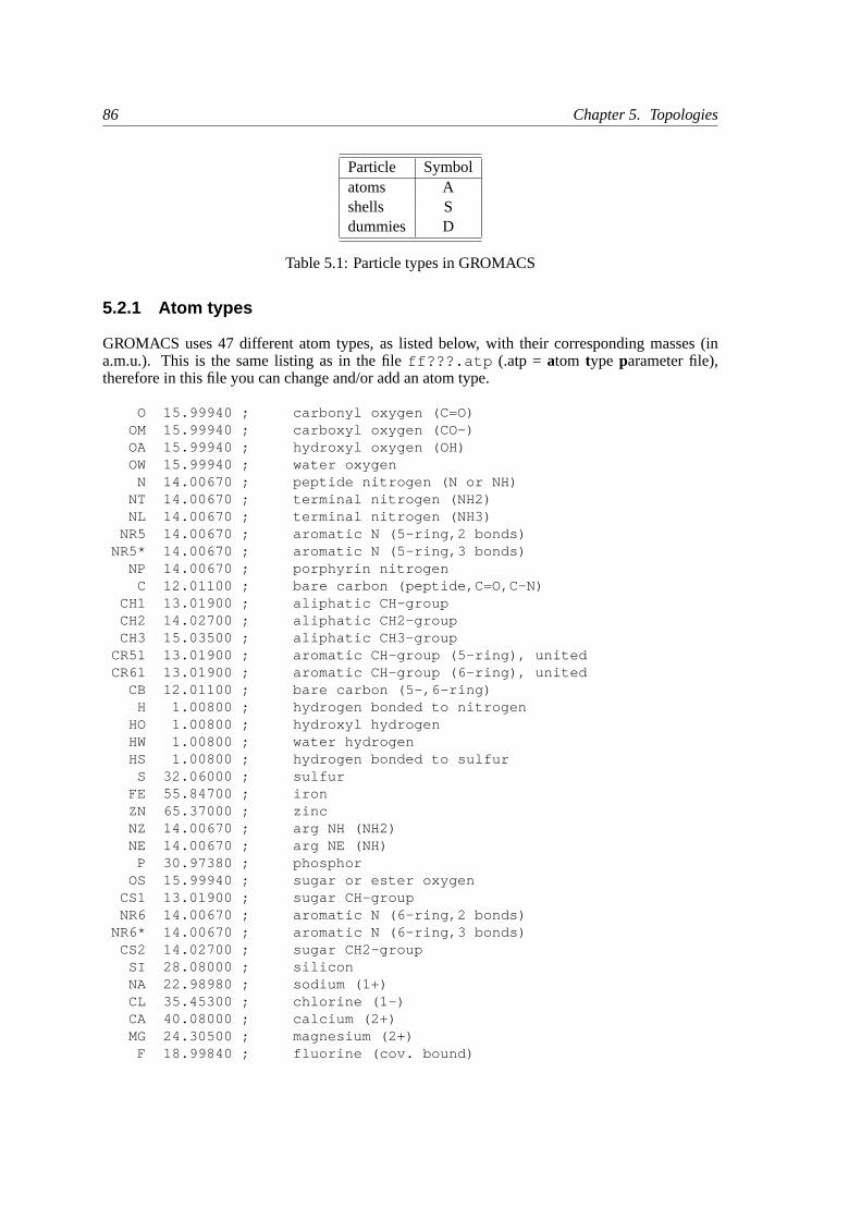
86 Chapter 5. Topologies
Particle Symbolatoms Ashells Sdummies D
Table 5.1: Particle types in GROMACS
5.2.1 Atom types
GROMACS uses 47 different atom types, as listed below, with their corresponding masses (ina.m.u.). This is the same listing as in the fileff???.atp (.atp = atom type parameter file),therefore in this file you can change and/or add an atom type.
O 15.99940 ; carbonyl oxygen (C=O)OM 15.99940 ; carboxyl oxygen (CO-)OA 15.99940 ; hydroxyl oxygen (OH)OW 15.99940 ; water oxygen
N 14.00670 ; peptide nitrogen (N or NH)NT 14.00670 ; terminal nitrogen (NH2)NL 14.00670 ; terminal nitrogen (NH3)
NR5 14.00670 ; aromatic N (5-ring,2 bonds)NR5* 14.00670 ; aromatic N (5-ring,3 bonds)
NP 14.00670 ; porphyrin nitrogenC 12.01100 ; bare carbon (peptide,C=O,C-N)
CH1 13.01900 ; aliphatic CH-groupCH2 14.02700 ; aliphatic CH2-groupCH3 15.03500 ; aliphatic CH3-group
CR51 13.01900 ; aromatic CH-group (5-ring), unitedCR61 13.01900 ; aromatic CH-group (6-ring), united
CB 12.01100 ; bare carbon (5-,6-ring)H 1.00800 ; hydrogen bonded to nitrogen
HO 1.00800 ; hydroxyl hydrogenHW 1.00800 ; water hydrogenHS 1.00800 ; hydrogen bonded to sulfur
S 32.06000 ; sulfurFE 55.84700 ; ironZN 65.37000 ; zincNZ 14.00670 ; arg NH (NH2)NE 14.00670 ; arg NE (NH)
P 30.97380 ; phosphorOS 15.99940 ; sugar or ester oxygen
CS1 13.01900 ; sugar CH-groupNR6 14.00670 ; aromatic N (6-ring,2 bonds)
NR6* 14.00670 ; aromatic N (6-ring,3 bonds)CS2 14.02700 ; sugar CH2-group
SI 28.08000 ; siliconNA 22.98980 ; sodium (1+)CL 35.45300 ; chlorine (1-)CA 40.08000 ; calcium (2+)MG 24.30500 ; magnesium (2+)
F 18.99840 ; fluorine (cov. bound)

5.2. Particle type 87
CP2 14.02700 ; aliphatic CH2-group using Ryckaert-Bell.CP3 15.03500 ; aliphatic CH3-group using Ryckaert-Bell.CR5 12.01100 ; aromatic CH-group (5-ring)+HCR6 12.01100 ; aromatic C- bonded to H (6-ring)+HHCR 1.00800 ; H attached to aromatic C (5 or 6 ri
OWT3 15.99940 ; TIP3P water oxygenSD 32.06000 ; DMSO SulphurOD 15.99940 ; DMSO OxygenCD 15.03500 ; DMSO Carbon
Atomic detail is used except for hydrogen atoms bound to (aliphatic) carbon atoms, which aretreated asunited atoms. No special hydrogen-bond term is included.
The last 10 atom types are extra atom types with respect to the GROMOS-87 force field [39]:
• F was taken from ref. [43],
• CP2 and CP3 from ref. [40] and references cited therein,
• CR5, CR6 and HCR from ref. [59]
• OWT3 from ref. [42]
• SD, OD and CD from ref. [44]
Therefore, if you use the GROMACS force field as it is, be sure to include these references inyour publications.
Note: GROMACS makes use of the atom types as a name,notas a number (ase.g.in GROMOS).
5.2.2 Dummy atoms
Some force fields use dummy atoms (virtual sites that are constructed from real atoms) on whichcertain interactions are located (e.g.on benzene rings, to reproduce the correct quadrupole). Thisis described in sec.4.5.
To make dummy atoms in your system, you should include a section[ dummies? ] in yourtopology file, where the ‘?’ stands for the number constructing atoms for the dummy atom. Thiswill be ‘2’ for type 2, ‘3’ for types 3, 3fd, 3fad and 3out and ‘4’ for type 4fd (the different typesare explained in sec.4.5).
Parameters for type 2 should look like this:
[ dummies2 ]; Dummy from funct a5 1 2 1 0.7439756
for type 3 like this:
[ dummies3 ]; Dummy from funct a b5 1 2 3 1 0.7439756 0.128012
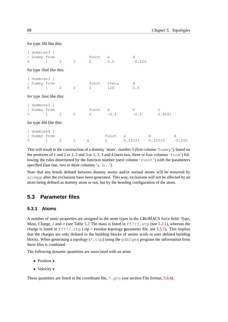
88 Chapter 5. Topologies
for type 3fd like this:
[ dummies3 ]; Dummy from funct a d5 1 2 3 2 0.5 -0.105
for type 3fad like this:
[ dummies3 ]; Dummy from funct theta d5 1 2 3 3 120 0.5
for type 3out like this:
[ dummies3 ]; Dummy from funct a b c5 1 2 3 4 -0.4 -0.4 6.9281
for type 4fd like this:
[ dummies4 ]; Dummy from funct a b d5 1 2 3 4 1 0.33333 0.33333 -0.105
This will result in the construction of a dummy ‘atom’, number 5 (first column ‘Dummy’), based onthe positions of 1 and 2 or 1, 2 and 3 or 1, 2, 3 and 4 (next two, three or four columns ‘from ’) fol-lowing the rules determined by the function number (next column ‘funct ’) with the parametersspecified (last one, two or three columns ‘a b . .’).
Note that any bonds defined between dummy atoms and/or normal atoms will be removed bygrompp after the exclusions have been generated. This way, exclusions will not be affected by anatom being defined as dummy atom or not, but by the bonding configuration of the atom.
5.3 Parameter files
5.3.1 Atoms
A number ofstaticproperties are assigned to the atom types in the GROMACS force field: Type,Mass, Charge,ε andσ (see Table5.2The mass is listed inff???.atp (see5.2.1), whereas thecharge is listed inff???.rtp (.rtp = residuetopologyparameter file, see5.5.1). This impliesthat the charges are only defined in the building blocks of amino acids or user defined buildingblocks. When generating a topology (*.top ) using thepdb2gmx program the information fromthese files is combined.
The followingdynamicquantities are associated with an atom
• Positionx
• Velocity v
These quantities are listed in the coordinate file,*.gro (see section File format,5.6.6).
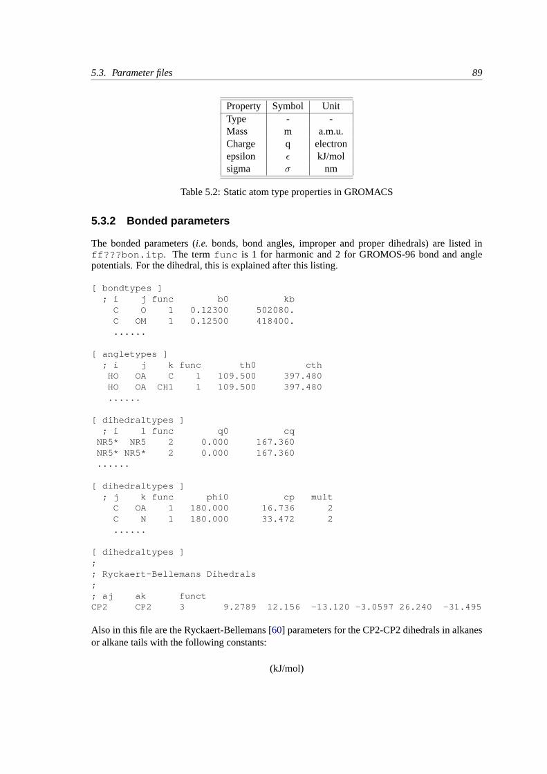
5.3. Parameter files 89
Property Symbol UnitType - -Mass m a.m.u.Charge q electronepsilon ε kJ/molsigma σ nm
Table 5.2: Static atom type properties in GROMACS
5.3.2 Bonded parameters
The bonded parameters (i.e. bonds, bond angles, improper and proper dihedrals) are listed inff???bon.itp . The termfunc is 1 for harmonic and 2 for GROMOS-96 bond and anglepotentials. For the dihedral, this is explained after this listing.
[ bondtypes ]; i j func b0 kb
C O 1 0.12300 502080.C OM 1 0.12500 418400.......
[ angletypes ]; i j k func th0 cth
HO OA C 1 109.500 397.480HO OA CH1 1 109.500 397.480......
[ dihedraltypes ]; i l func q0 cq
NR5* NR5 2 0.000 167.360NR5* NR5* 2 0.000 167.360......
[ dihedraltypes ]; j k func phi0 cp mult
C OA 1 180.000 16.736 2C N 1 180.000 33.472 2......
[ dihedraltypes ];; Ryckaert-Bellemans Dihedrals;; aj ak functCP2 CP2 3 9.2789 12.156 -13.120 -3.0597 26.240 -31.495
Also in this file are the Ryckaert-Bellemans [60] parameters for the CP2-CP2 dihedrals in alkanesor alkane tails with the following constants:
(kJ/mol)
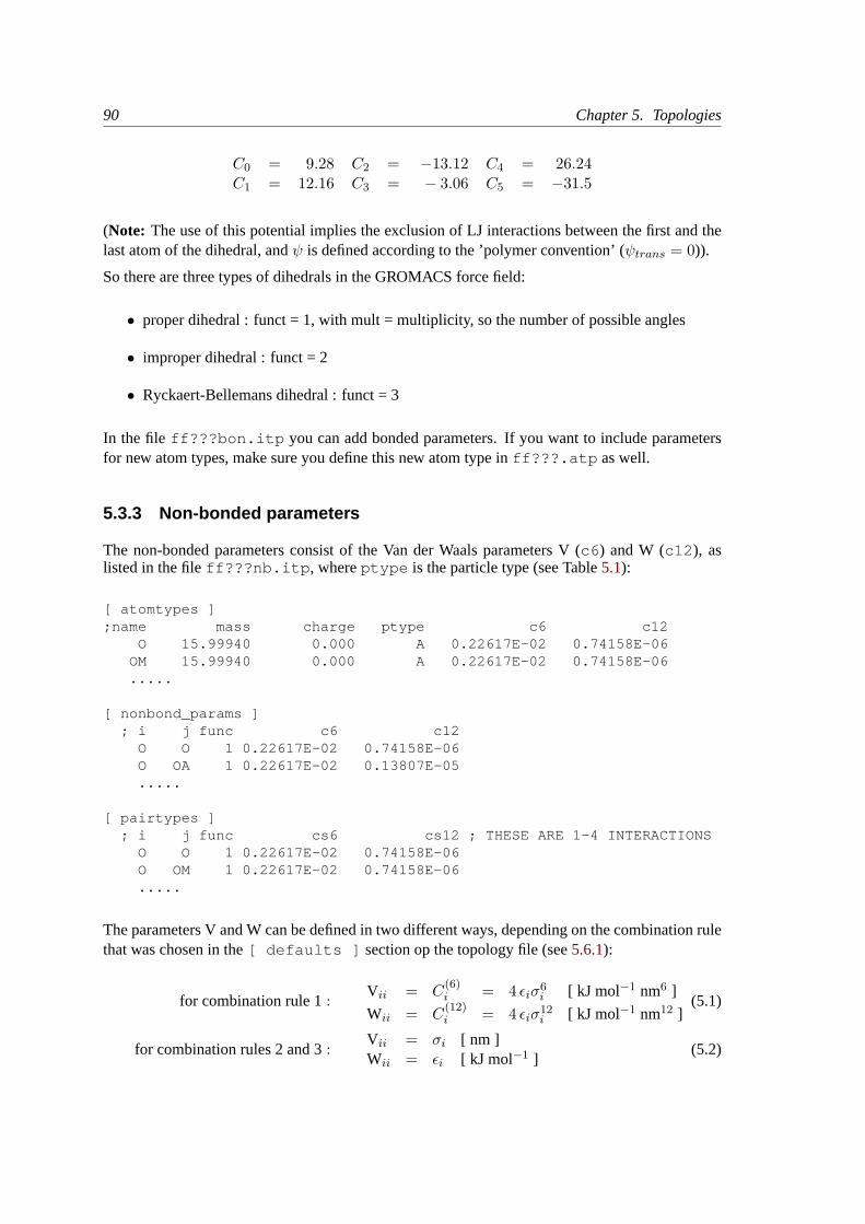
90 Chapter 5. Topologies
C0 = 9.28 C2 = −13.12 C4 = 26.24C1 = 12.16 C3 = − 3.06 C5 = −31.5
(Note: The use of this potential implies the exclusion of LJ interactions between the first and thelast atom of the dihedral, andψ is defined according to the ’polymer convention’ (ψtrans = 0)).
So there are three types of dihedrals in the GROMACS force field:
• proper dihedral : funct = 1, with mult = multiplicity, so the number of possible angles
• improper dihedral : funct = 2
• Ryckaert-Bellemans dihedral : funct = 3
In the file ff???bon.itp you can add bonded parameters. If you want to include parametersfor new atom types, make sure you define this new atom type inff???.atp as well.
5.3.3 Non-bonded parameters
The non-bonded parameters consist of the Van der Waals parameters V (c6 ) and W (c12 ), aslisted in the fileff???nb.itp , whereptype is the particle type (see Table5.1):
[ atomtypes ];name mass charge ptype c6 c12
O 15.99940 0.000 A 0.22617E-02 0.74158E-06OM 15.99940 0.000 A 0.22617E-02 0.74158E-06.....
[ nonbond_params ]; i j func c6 c12
O O 1 0.22617E-02 0.74158E-06O OA 1 0.22617E-02 0.13807E-05.....
[ pairtypes ]; i j func cs6 cs12 ; THESE ARE 1-4 INTERACTIONS
O O 1 0.22617E-02 0.74158E-06O OM 1 0.22617E-02 0.74158E-06.....
The parameters V and W can be defined in two different ways, depending on the combination rulethat was chosen in the[ defaults ] section op the topology file (see5.6.1):
for combination rule 1:Vii = C
(6)i = 4 εiσ6
i [ kJ mol−1 nm6 ]
Wii = C(12)i = 4 εiσ12
i [ kJ mol−1 nm12 ](5.1)
for combination rules 2 and 3:Vii = σi [ nm ]Wii = εi [ kJ mol−1 ]
(5.2)
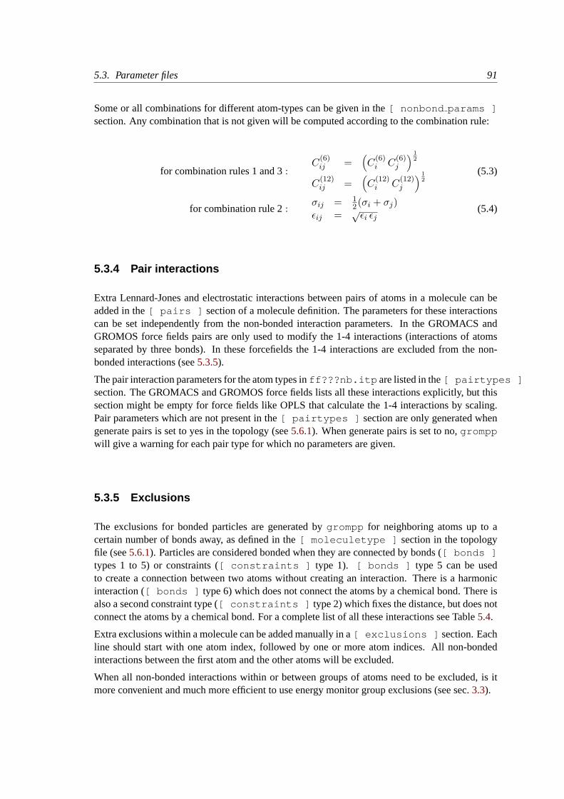
5.3. Parameter files 91
Some or all combinations for different atom-types can be given in the[ nonbond params ]section. Any combination that is not given will be computed according to the combination rule:
for combination rules 1 and 3:C
(6)ij =
(C
(6)i C
(6)j
) 12
C(12)ij =
(C
(12)i C
(12)j
) 12
(5.3)
for combination rule 2:σij = 1
2(σi + σj)εij = √
εi εj(5.4)
5.3.4 Pair interactions
Extra Lennard-Jones and electrostatic interactions between pairs of atoms in a molecule can beadded in the[ pairs ] section of a molecule definition. The parameters for these interactionscan be set independently from the non-bonded interaction parameters. In the GROMACS andGROMOS force fields pairs are only used to modify the 1-4 interactions (interactions of atomsseparated by three bonds). In these forcefields the 1-4 interactions are excluded from the non-bonded interactions (see5.3.5).
The pair interaction parameters for the atom types inff???nb.itp are listed in the[ pairtypes ]section. The GROMACS and GROMOS force fields lists all these interactions explicitly, but thissection might be empty for force fields like OPLS that calculate the 1-4 interactions by scaling.Pair parameters which are not present in the[ pairtypes ] section are only generated whengenerate pairs is set to yes in the topology (see5.6.1). When generate pairs is set to no,gromppwill give a warning for each pair type for which no parameters are given.
5.3.5 Exclusions
The exclusions for bonded particles are generated bygrompp for neighboring atoms up to acertain number of bonds away, as defined in the[ moleculetype ] section in the topologyfile (see5.6.1). Particles are considered bonded when they are connected by bonds ([ bonds ]types 1 to 5) or constraints ([ constraints ] type 1). [ bonds ] type 5 can be usedto create a connection between two atoms without creating an interaction. There is a harmonicinteraction ([ bonds ] type 6) which does not connect the atoms by a chemical bond. There isalso a second constraint type ([ constraints ] type 2) which fixes the distance, but does notconnect the atoms by a chemical bond. For a complete list of all these interactions see Table5.4.
Extra exclusions within a molecule can be added manually in a[ exclusions ] section. Eachline should start with one atom index, followed by one or more atom indices. All non-bondedinteractions between the first atom and the other atoms will be excluded.
When all non-bonded interactions within or between groups of atoms need to be excluded, is itmore convenient and much more efficient to use energy monitor group exclusions (see sec.3.3).
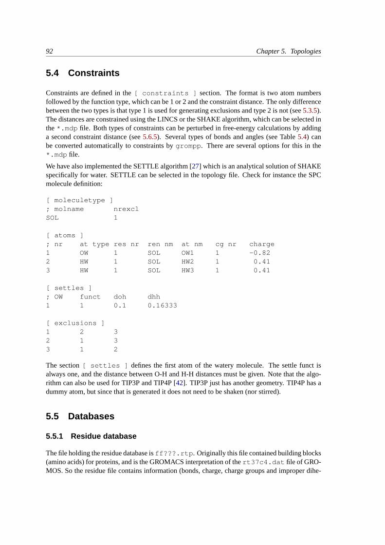
92 Chapter 5. Topologies
5.4 Constraints
Constraints are defined in the[ constraints ] section. The format is two atom numbersfollowed by the function type, which can be 1 or 2 and the constraint distance. The only differencebetween the two types is that type 1 is used for generating exclusions and type 2 is not (see5.3.5).The distances are constrained using the LINCS or the SHAKE algorithm, which can be selected inthe*.mdp file. Both types of constraints can be perturbed in free-energy calculations by addinga second constraint distance (see5.6.5). Several types of bonds and angles (see Table5.4) canbe converted automatically to constraints bygrompp . There are several options for this in the*.mdp file.
We have also implemented the SETTLE algorithm [27] which is an analytical solution of SHAKEspecifically for water. SETTLE can be selected in the topology file. Check for instance the SPCmolecule definition:
[ moleculetype ]; molname nrexclSOL 1
[ atoms ]; nr at type res nr ren nm at nm cg nr charge1 OW 1 SOL OW1 1 -0.822 HW 1 SOL HW2 1 0.413 HW 1 SOL HW3 1 0.41
[ settles ]; OW funct doh dhh1 1 0.1 0.16333
[ exclusions ]1 2 32 1 33 1 2
The section[ settles ] defines the first atom of the watery molecule. The settle funct isalways one, and the distance between O-H and H-H distances must be given. Note that the algo-rithm can also be used for TIP3P and TIP4P [42]. TIP3P just has another geometry. TIP4P has adummy atom, but since that is generated it does not need to be shaken (nor stirred).
5.5 Databases
5.5.1 Residue database
The file holding the residue database isff???.rtp . Originally this file contained building blocks(amino acids) for proteins, and is the GROMACS interpretation of thert37c4.dat file of GRO-MOS. So the residue file contains information (bonds, charge, charge groups and improper dihe-
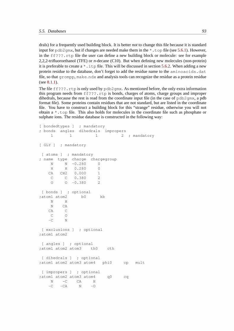
5.5. Databases 93
drals) for a frequently used building block. It is betternot to change this file because it is standardinput forpdb2gmx , but if changes are needed make them in the*.top file (see5.6.1). However,in the ff???.rtp file the user can define a new building block or molecule: see for example2,2,2-trifluoroethanol (TFE) orn-decane (C10). But when defining new molecules (non-protein)it is preferable to create a*.itp file. This will be discussed in section5.6.2. When adding a newprotein residue to the database, don’t forget to add the residue name to theaminoacids.datfile, so thatgrompp , make ndx and analysis tools can recognize the residue as a protein residue(see8.1.1).
The fileff???.rtp is only used bypdb2gmx . As mentioned before, the only extra informationthis program needs fromff???.rtp is bonds, charges of atoms, charge groups and improperdihedrals, because the rest is read from the coordinate input file (in the case ofpdb2gmx , a pdbformat file). Some proteins contain residues that are not standard, but are listed in the coordinatefile. You have to construct a building block for this “strange” residue, otherwise you will notobtain a*.top file. This also holds for molecules in the coordinate file such as phosphate orsulphate ions. The residue database is constructed in the following way:
[ bondedtypes ] ; mandatory; bonds angles dihedrals impropers
1 1 1 2 ; mandatory
[ GLY ] ; mandatory
[ atoms ] ; mandatory; name type charge chargegroup
N N -0.280 0H H 0.280 0
CA CH2 0.000 1C C 0.380 2O O -0.380 2
[ bonds ] ; optional;atom1 atom2 b0 kb
N HN CA
CA CC O
-C N
[ exclusions ] ; optional;atom1 atom2
[ angles ] ; optional;atom1 atom2 atom3 th0 cth
[ dihedrals ] ; optional;atom1 atom2 atom3 atom4 phi0 cp mult
[ impropers ] ; optional;atom1 atom2 atom3 atom4 q0 cq
N -C CA H-C -CA N -O
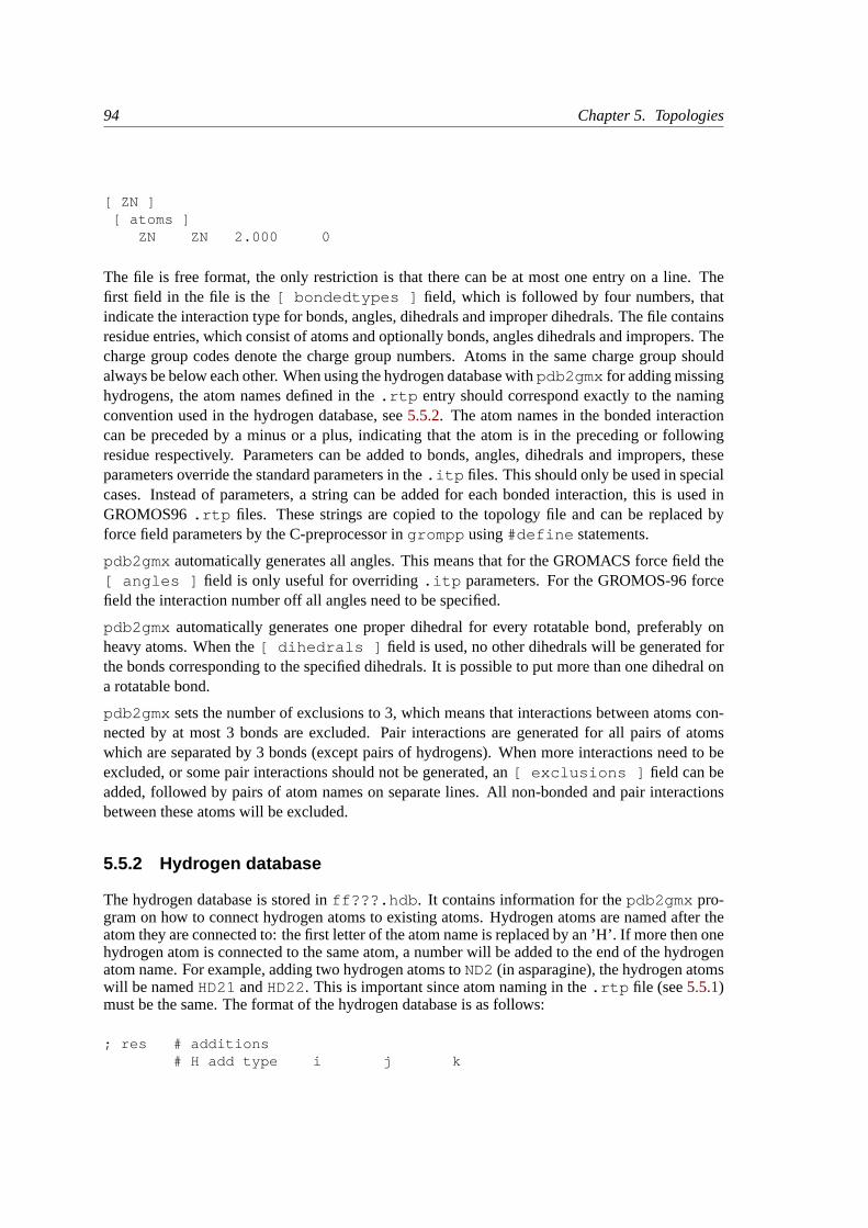
94 Chapter 5. Topologies
[ ZN ][ atoms ]
ZN ZN 2.000 0
The file is free format, the only restriction is that there can be at most one entry on a line. Thefirst field in the file is the[ bondedtypes ] field, which is followed by four numbers, thatindicate the interaction type for bonds, angles, dihedrals and improper dihedrals. The file containsresidue entries, which consist of atoms and optionally bonds, angles dihedrals and impropers. Thecharge group codes denote the charge group numbers. Atoms in the same charge group shouldalways be below each other. When using the hydrogen database withpdb2gmx for adding missinghydrogens, the atom names defined in the.rtp entry should correspond exactly to the namingconvention used in the hydrogen database, see5.5.2. The atom names in the bonded interactioncan be preceded by a minus or a plus, indicating that the atom is in the preceding or followingresidue respectively. Parameters can be added to bonds, angles, dihedrals and impropers, theseparameters override the standard parameters in the.itp files. This should only be used in specialcases. Instead of parameters, a string can be added for each bonded interaction, this is used inGROMOS96.rtp files. These strings are copied to the topology file and can be replaced byforce field parameters by the C-preprocessor ingrompp using#define statements.
pdb2gmx automatically generates all angles. This means that for the GROMACS force field the[ angles ] field is only useful for overriding.itp parameters. For the GROMOS-96 forcefield the interaction number off all angles need to be specified.
pdb2gmx automatically generates one proper dihedral for every rotatable bond, preferably onheavy atoms. When the[ dihedrals ] field is used, no other dihedrals will be generated forthe bonds corresponding to the specified dihedrals. It is possible to put more than one dihedral ona rotatable bond.
pdb2gmx sets the number of exclusions to 3, which means that interactions between atoms con-nected by at most 3 bonds are excluded. Pair interactions are generated for all pairs of atomswhich are separated by 3 bonds (except pairs of hydrogens). When more interactions need to beexcluded, or some pair interactions should not be generated, an[ exclusions ] field can beadded, followed by pairs of atom names on separate lines. All non-bonded and pair interactionsbetween these atoms will be excluded.
5.5.2 Hydrogen database
The hydrogen database is stored inff???.hdb . It contains information for thepdb2gmx pro-gram on how to connect hydrogen atoms to existing atoms. Hydrogen atoms are named after theatom they are connected to: the first letter of the atom name is replaced by an ’H’. If more then onehydrogen atom is connected to the same atom, a number will be added to the end of the hydrogenatom name. For example, adding two hydrogen atoms toND2(in asparagine), the hydrogen atomswill be namedHD21andHD22. This is important since atom naming in the.rtp file (see5.5.1)must be the same. The format of the hydrogen database is as follows:
; res # additions# H add type i j k
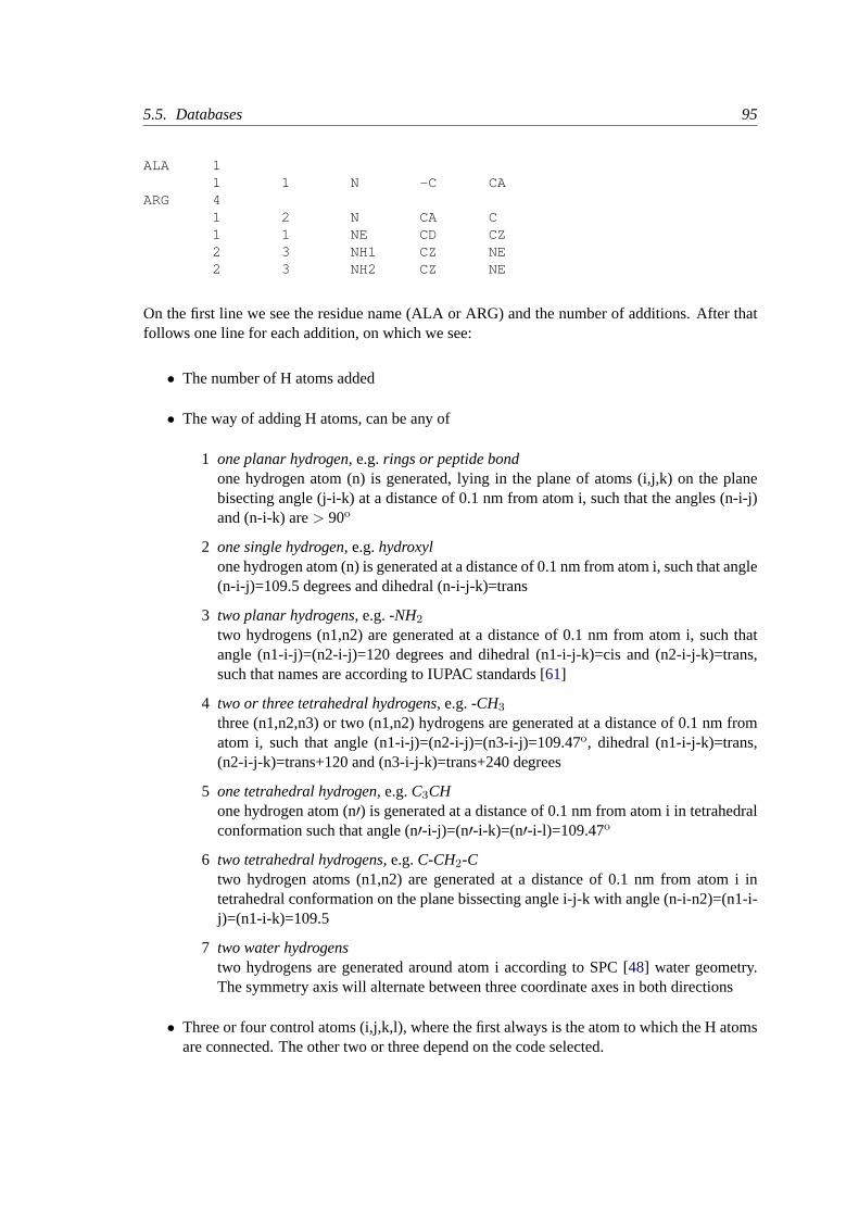
5.5. Databases 95
ALA 11 1 N -C CA
ARG 41 2 N CA C1 1 NE CD CZ2 3 NH1 CZ NE2 3 NH2 CZ NE
On the first line we see the residue name (ALA or ARG) and the number of additions. After thatfollows one line for each addition, on which we see:
• The number of H atoms added
• The way of adding H atoms, can be any of
1 one planar hydrogen,e.g.rings or peptide bondone hydrogen atom (n) is generated, lying in the plane of atoms (i,j,k) on the planebisecting angle (j-i-k) at a distance of 0.1 nm from atom i, such that the angles (n-i-j)and (n-i-k) are> 90o
2 one single hydrogen,e.g.hydroxylone hydrogen atom (n) is generated at a distance of 0.1 nm from atom i, such that angle(n-i-j)=109.5 degrees and dihedral (n-i-j-k)=trans
3 two planar hydrogens,e.g.-NH2
two hydrogens (n1,n2) are generated at a distance of 0.1 nm from atom i, such thatangle (n1-i-j)=(n2-i-j)=120 degrees and dihedral (n1-i-j-k)=cis and (n2-i-j-k)=trans,such that names are according to IUPAC standards [61]
4 two or three tetrahedral hydrogens,e.g.-CH3
three (n1,n2,n3) or two (n1,n2) hydrogens are generated at a distance of 0.1 nm fromatom i, such that angle (n1-i-j)=(n2-i-j)=(n3-i-j)=109.47o, dihedral (n1-i-j-k)=trans,(n2-i-j-k)=trans+120 and (n3-i-j-k)=trans+240 degrees
5 one tetrahedral hydrogen,e.g.C3CHone hydrogen atom (n′) is generated at a distance of 0.1 nm from atom i in tetrahedralconformation such that angle (n′-i-j)=(n′-i-k)=(n′-i-l)=109.47o
6 two tetrahedral hydrogens,e.g.C-CH2-Ctwo hydrogen atoms (n1,n2) are generated at a distance of 0.1 nm from atom i intetrahedral conformation on the plane bissecting angle i-j-k with angle (n-i-n2)=(n1-i-j)=(n1-i-k)=109.5
7 two water hydrogenstwo hydrogens are generated around atom i according to SPC [48] water geometry.The symmetry axis will alternate between three coordinate axes in both directions
• Three or four control atoms (i,j,k,l), where the first always is the atom to which the H atomsare connected. The other two or three depend on the code selected.
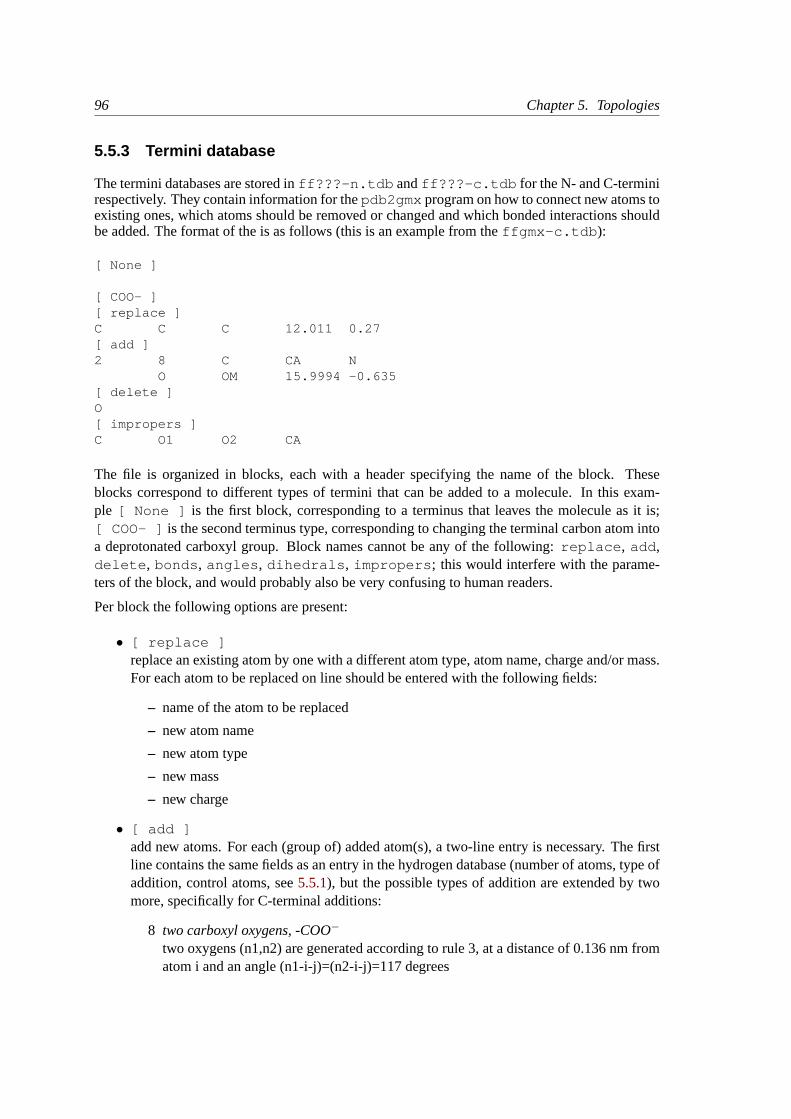
96 Chapter 5. Topologies
5.5.3 Termini database
The termini databases are stored inff???-n.tdb andff???-c.tdb for the N- and C-terminirespectively. They contain information for thepdb2gmx program on how to connect new atoms toexisting ones, which atoms should be removed or changed and which bonded interactions shouldbe added. The format of the is as follows (this is an example from theffgmx-c.tdb ):
[ None ]
[ COO- ][ replace ]C C C 12.011 0.27[ add ]2 8 C CA N
O OM 15.9994 -0.635[ delete ]O[ impropers ]C O1 O2 CA
The file is organized in blocks, each with a header specifying the name of the block. Theseblocks correspond to different types of termini that can be added to a molecule. In this exam-ple [ None ] is the first block, corresponding to a terminus that leaves the molecule as it is;[ COO- ] is the second terminus type, corresponding to changing the terminal carbon atom intoa deprotonated carboxyl group. Block names cannot be any of the following:replace , add ,delete , bonds , angles , dihedrals , impropers ; this would interfere with the parame-ters of the block, and would probably also be very confusing to human readers.
Per block the following options are present:
• [ replace ]replace an existing atom by one with a different atom type, atom name, charge and/or mass.For each atom to be replaced on line should be entered with the following fields:
– name of the atom to be replaced
– new atom name
– new atom type
– new mass
– new charge
• [ add ]add new atoms. For each (group of) added atom(s), a two-line entry is necessary. The firstline contains the same fields as an entry in the hydrogen database (number of atoms, type ofaddition, control atoms, see5.5.1), but the possible types of addition are extended by twomore, specifically for C-terminal additions:
8 two carboxyl oxygens, -COO−
two oxygens (n1,n2) are generated according to rule 3, at a distance of 0.136 nm fromatom i and an angle (n1-i-j)=(n2-i-j)=117 degrees
5.6. File formats 97
9 carboxyl oxygens and hydrogen, -COOHtwo oxygens (n1,n2) are generated according to rule 3, at distances of 0.123 nm and0.125 nm from atom i for n1 and n2 resp. and angles (n1-i-j)=121 and (n2-i-j)=115degrees. One hydrogen (n’) is generated around n2 according to rule 2, where n-i-jand n-i-j-k should be read as n’-n2-i and n’-n2-i-j resp.
After this line another line follows which specifies the details of the added atom(s), in thesame way as for replacing atoms,i.e.:
– atom name
– atom type
– mass
– charge
Like in the hydrogen database (see5.5.1), when more then one atom is connected to anexisting one, a number will be appended to the end of the atom name.
• [ delete ]delete existing atoms. One atom name per line.
• [ bonds ] , [ angles ] , [ dihedrals ] and[ impropers ]add additional bonded parameters. The format is identical to that used in theff???.rtp ,see5.5.1.
5.6 File formats
5.6.1 Topology file
The topology file is built following the GROMACS specification for a molecular topology. A*.top file can be generated bypdb2gmx . All possible entries in the topology file are listed inTable5.3 and Table5.4. Also listed are all the units of the parameters, which interactions canbe perturbed for free energy calculations, which bonded interactions are used bygrompp forgenerating exclusions and which bonded interactions can be converted to constraints bygrompp .
Description of the file layout:
• semicolon (;) and newline surround comments
• on a line ending with\ the newline character is ignored.
• directives are surrounded by[ and]
• the topology consists of three levels:
– the parameter level (see Table5.3)
– the molecule level, which should contain one or more molecule definitions (see Ta-ble5.4)
– the system level:[ system ] , [ molecules ]
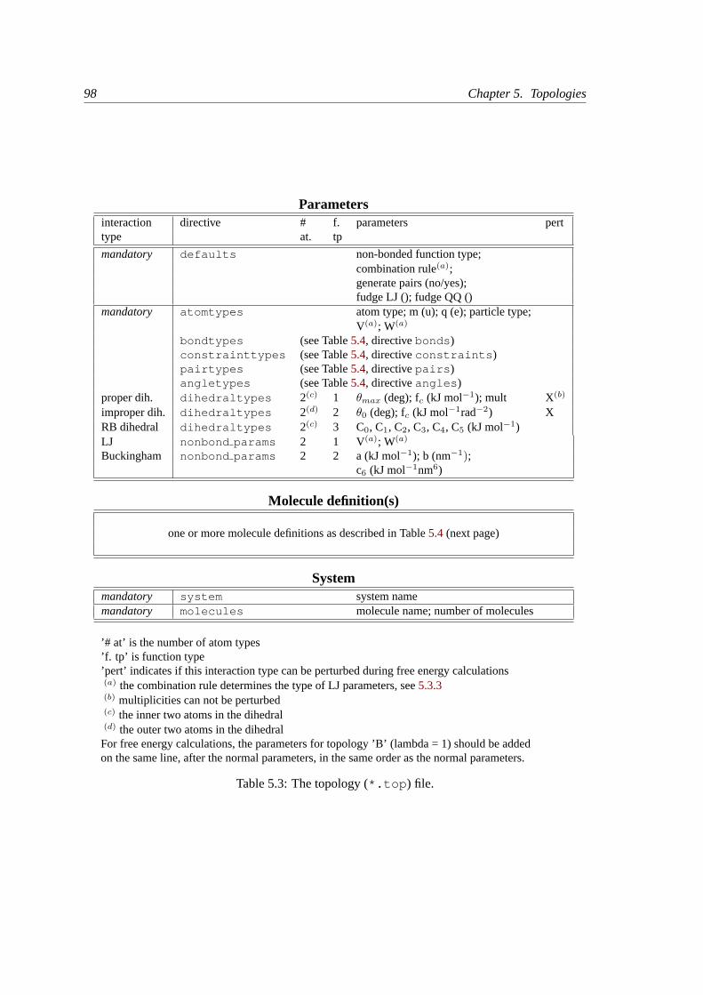
98 Chapter 5. Topologies
Parametersinteraction directive # f. parameters perttype at. tp
mandatory defaults non-bonded function type;combination rule(a);generate pairs (no/yes);fudge LJ (); fudge QQ ()
mandatory atomtypes atom type; m (u); q (e); particle type;V(a); W(a)
bondtypes (see Table5.4, directivebonds )constrainttypes (see Table5.4, directiveconstraints )pairtypes (see Table5.4, directivepairs )angletypes (see Table5.4, directiveangles )
proper dih. dihedraltypes 2(c) 1 θmax (deg); fc (kJ mol−1); mult X(b)
improper dih. dihedraltypes 2(d) 2 θ0 (deg); fc (kJ mol−1rad−2) XRB dihedral dihedraltypes 2(c) 3 C0, C1, C2, C3, C4, C5 (kJ mol−1)LJ nonbond params 2 1 V(a); W(a)
Buckingham nonbond params 2 2 a (kJ mol−1); b (nm−1);c6 (kJ mol−1nm6)
Molecule definition(s)
one or more molecule definitions as described in Table5.4(next page)
Systemmandatory system system namemandatory molecules molecule name; number of molecules
’# at’ is the number of atom types’f. tp’ is function type’pert’ indicates if this interaction type can be perturbed during free energy calculations(a) the combination rule determines the type of LJ parameters, see5.3.3(b) multiplicities can not be perturbed(c) the inner two atoms in the dihedral(d) the outer two atoms in the dihedralFor free energy calculations, the parameters for topology ’B’ (lambda = 1) should be addedon the same line, after the normal parameters, in the same order as the normal parameters.
Table 5.3: The topology (*.top ) file.
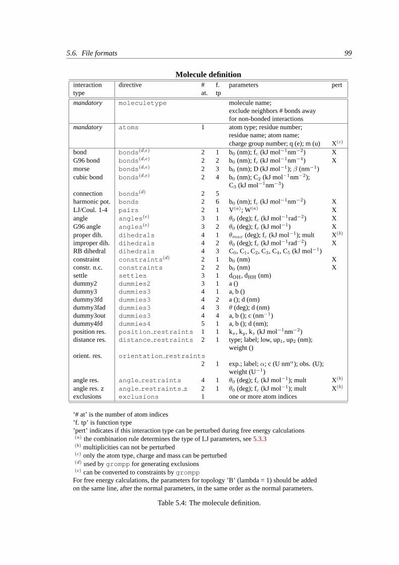
5.6. File formats 99
Molecule definitioninteraction directive # f. parameters perttype at. tp
mandatory moleculetype molecule name;exclude neighbors # bonds awayfor non-bonded interactions
mandatory atoms 1 atom type; residue number;residue name; atom name;charge group number; q (e); m (u) X(c)
bond bonds (d,e) 2 1 b0 (nm); fc (kJ mol−1nm−2) XG96 bond bonds (d,e) 2 2 b0 (nm); fc (kJ mol−1nm−4) Xmorse bonds (d,e) 2 3 b0 (nm); D (kJ mol−1); β (nm−1)cubic bond bonds (d,e) 2 4 b0 (nm); C2 (kJ mol−1nm−2);
C3 (kJ mol−1nm−3)connection bonds (d) 2 5harmonic pot. bonds 2 6 b0 (nm); fc (kJ mol−1nm−2) XLJ/Coul. 1-4 pairs 2 1 V(a); W(a) Xangle angles (e) 3 1 θ0 (deg); fc (kJ mol−1rad−2) XG96 angle angles (e) 3 2 θ0 (deg); fc (kJ mol−1) Xproper dih. dihedrals 4 1 θmax (deg); fc (kJ mol−1); mult X(b)
improper dih. dihedrals 4 2 θ0 (deg); fc (kJ mol−1rad−2) XRB dihedral dihedrals 4 3 C0, C1, C2, C3, C4, C5 (kJ mol−1)constraint constraints (d) 2 1 b0 (nm) Xconstr. n.c. constraints 2 2 b0 (nm) Xsettle settles 3 1 dOH, dHH (nm)dummy2 dummies2 3 1 a ()dummy3 dummies3 4 1 a, b ()dummy3fd dummies3 4 2 a (); d (nm)dummy3fad dummies3 4 3 θ (deg); d (nm)dummy3out dummies3 4 4 a, b (); c (nm−1)dummy4fd dummies4 5 1 a, b (); d (nm);position res. position restraints 1 1 kx, ky, kz (kJ mol−1nm−2)distance res. distance restraints 2 1 type; label; low, up1, up2 (nm);
weight ()orient. res. orientation restraints
2 1 exp.; label;α; c (U nmα); obs. (U);weight (U−1)
angle res. angle restraints 4 1 θ0 (deg); fc (kJ mol−1); mult X(b)
angle res. z angle restraints z 2 1 θ0 (deg); fc (kJ mol−1); mult X(b)
exclusions exclusions 1 one or more atom indices
’# at’ is the number of atom indices’f. tp’ is function type’pert’ indicates if this interaction type can be perturbed during free energy calculations(a) the combination rule determines the type of LJ parameters, see5.3.3(b) multiplicities can not be perturbed(c) only the atom type, charge and mass can be perturbed(d) used bygrompp for generating exclusions(e) can be converted to constraints bygromppFor free energy calculations, the parameters for topology ’B’ (lambda = 1) should be addedon the same line, after the normal parameters, in the same order as the normal parameters.
Table 5.4: The molecule definition.
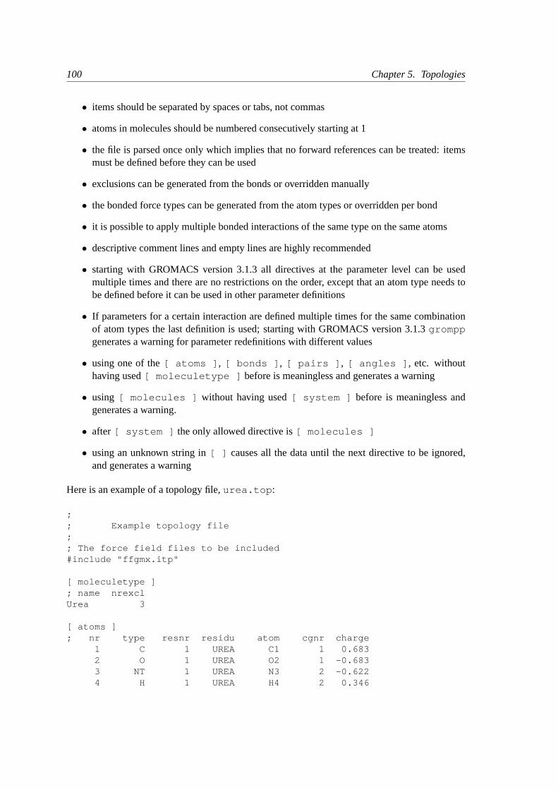
100 Chapter 5. Topologies
• items should be separated by spaces or tabs, not commas
• atoms in molecules should be numbered consecutively starting at 1
• the file is parsed once only which implies that no forward references can be treated: itemsmust be defined before they can be used
• exclusions can be generated from the bonds or overridden manually
• the bonded force types can be generated from the atom types or overridden per bond
• it is possible to apply multiple bonded interactions of the same type on the same atoms
• descriptive comment lines and empty lines are highly recommended
• starting with GROMACS version 3.1.3 all directives at the parameter level can be usedmultiple times and there are no restrictions on the order, except that an atom type needs tobe defined before it can be used in other parameter definitions
• If parameters for a certain interaction are defined multiple times for the same combinationof atom types the last definition is used; starting with GROMACS version 3.1.3gromppgenerates a warning for parameter redefinitions with different values
• using one of the[ atoms ] , [ bonds ] , [ pairs ] , [ angles ] , etc. withouthaving used[ moleculetype ] before is meaningless and generates a warning
• using [ molecules ] without having used[ system ] before is meaningless andgenerates a warning.
• after[ system ] the only allowed directive is[ molecules ]
• using an unknown string in[ ] causes all the data until the next directive to be ignored,and generates a warning
Here is an example of a topology file,urea.top :
;; Example topology file;; The force field files to be included#include "ffgmx.itp"
[ moleculetype ]; name nrexclUrea 3
[ atoms ]; nr type resnr residu atom cgnr charge
1 C 1 UREA C1 1 0.6832 O 1 UREA O2 1 -0.6833 NT 1 UREA N3 2 -0.6224 H 1 UREA H4 2 0.346
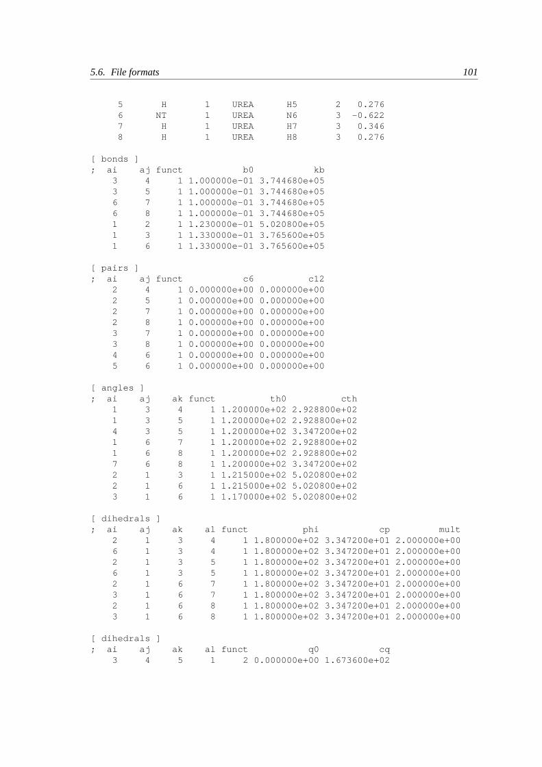
5.6. File formats 101
5 H 1 UREA H5 2 0.2766 NT 1 UREA N6 3 -0.6227 H 1 UREA H7 3 0.3468 H 1 UREA H8 3 0.276
[ bonds ]; ai aj funct b0 kb
3 4 1 1.000000e-01 3.744680e+053 5 1 1.000000e-01 3.744680e+056 7 1 1.000000e-01 3.744680e+056 8 1 1.000000e-01 3.744680e+051 2 1 1.230000e-01 5.020800e+051 3 1 1.330000e-01 3.765600e+051 6 1 1.330000e-01 3.765600e+05
[ pairs ]; ai aj funct c6 c12
2 4 1 0.000000e+00 0.000000e+002 5 1 0.000000e+00 0.000000e+002 7 1 0.000000e+00 0.000000e+002 8 1 0.000000e+00 0.000000e+003 7 1 0.000000e+00 0.000000e+003 8 1 0.000000e+00 0.000000e+004 6 1 0.000000e+00 0.000000e+005 6 1 0.000000e+00 0.000000e+00
[ angles ]; ai aj ak funct th0 cth
1 3 4 1 1.200000e+02 2.928800e+021 3 5 1 1.200000e+02 2.928800e+024 3 5 1 1.200000e+02 3.347200e+021 6 7 1 1.200000e+02 2.928800e+021 6 8 1 1.200000e+02 2.928800e+027 6 8 1 1.200000e+02 3.347200e+022 1 3 1 1.215000e+02 5.020800e+022 1 6 1 1.215000e+02 5.020800e+023 1 6 1 1.170000e+02 5.020800e+02
[ dihedrals ]; ai aj ak al funct phi cp mult
2 1 3 4 1 1.800000e+02 3.347200e+01 2.000000e+006 1 3 4 1 1.800000e+02 3.347200e+01 2.000000e+002 1 3 5 1 1.800000e+02 3.347200e+01 2.000000e+006 1 3 5 1 1.800000e+02 3.347200e+01 2.000000e+002 1 6 7 1 1.800000e+02 3.347200e+01 2.000000e+003 1 6 7 1 1.800000e+02 3.347200e+01 2.000000e+002 1 6 8 1 1.800000e+02 3.347200e+01 2.000000e+003 1 6 8 1 1.800000e+02 3.347200e+01 2.000000e+00
[ dihedrals ]; ai aj ak al funct q0 cq
3 4 5 1 2 0.000000e+00 1.673600e+02
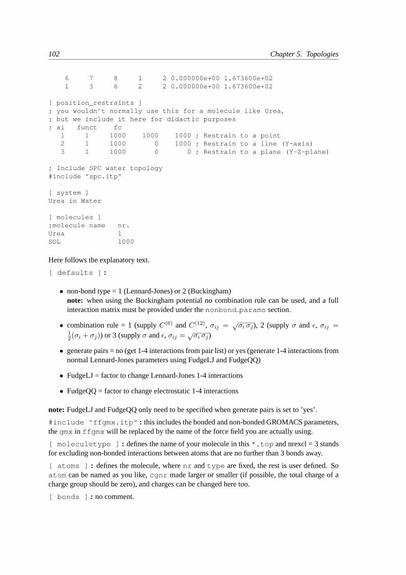
102 Chapter 5. Topologies
6 7 8 1 2 0.000000e+00 1.673600e+021 3 6 2 2 0.000000e+00 1.673600e+02
[ position_restraints ]; you wouldn’t normally use this for a molecule like Urea,; but we include it here for didactic purposes; ai funct fc
1 1 1000 1000 1000 ; Restrain to a point2 1 1000 0 1000 ; Restrain to a line (Y-axis)3 1 1000 0 0 ; Restrain to a plane (Y-Z-plane)
; Include SPC water topology#include "spc.itp"
[ system ]Urea in Water
[ molecules ];molecule name nr.Urea 1SOL 1000
Here follows the explanatory text.
[ defaults ] :
• non-bond type = 1 (Lennard-Jones) or 2 (Buckingham)note: when using the Buckingham potential no combination rule can be used, and a fullinteraction matrix must be provided under thenonbond params section.
• combination rule = 1 (supplyC(6) andC(12), σij = √σi σj), 2 (supplyσ and ε, σij =
12(σi + σj)) or 3 (supplyσ andε, σij = √
σi σj)
• generate pairs = no (get 1-4 interactions from pair list) or yes (generate 1-4 interactions fromnormal Lennard-Jones parameters using FudgeLJ and FudgeQQ)
• FudgeLJ = factor to change Lennard-Jones 1-4 interactions
• FudgeQQ = factor to change electrostatic 1-4 interactions
note: FudgeLJ and FudgeQQ only need to be specified when generate pairs is set to ’yes’.
#include "ffgmx.itp" : this includes the bonded and non-bonded GROMACS parameters,thegmx in ffgmx will be replaced by the name of the force field you are actually using.
[ moleculetype ] : defines the name of your molecule in this*.top and nrexcl = 3 standsfor excluding non-bonded interactions between atoms that are no further than 3 bonds away.
[ atoms ] : defines the molecule, wherenr andtype are fixed, the rest is user defined. Soatom can be named as you like,cgnr made larger or smaller (if possible, the total charge of acharge group should be zero), and charges can be changed here too.
[ bonds ] : no comment.
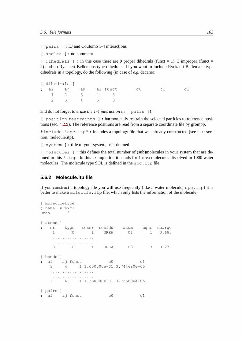
5.6. File formats 103
[ pairs ] : LJ and Coulomb 1-4 interactions
[ angles ] : no comment
[ dihedrals ] : in this case there are 9 proper dihedrals (funct = 1), 3 improper (funct =2) and no Ryckaert-Bellemans type dihedrals. If you want to include Ryckaert-Bellemans typedihedrals in a topology, do the following (in case ofe.g.decane):
[ dihedrals ]; ai aj ak al funct c0 c1 c2
1 2 3 4 32 3 4 5 3
and do not forget toerase the 1-4 interactionin [ pairs ] !!
[ position restraints ] : harmonically restrain the selected particles to reference posi-tions (sec.4.2.9). The reference positions are read from a separate coordinate file by grompp.
#include "spc.itp" : includes a topology file that was already constructed (see next sec-tion, molecule.itp).
[ system ] : title of your system, user defined
[ molecules ] : this defines the total number of (sub)molecules in your system that are de-fined in this*.top . In this example file it stands for 1 urea molecules dissolved in 1000 watermolecules. The molecule type SOL is defined in thespc.itp file.
5.6.2 Molecule.itp file
If you construct a topology file you will use frequently (like a water molecule,spc.itp ) it isbetter to make amolecule.itp file, which only lists the information of the molecule:
[ moleculetype ]; name nrexclUrea 3
[ atoms ]; nr type resnr residu atom cgnr charge
1 C 1 UREA C1 1 0.683..................................8 H 1 UREA H8 3 0.276
[ bonds ]; ai aj funct c0 c1
3 4 1 1.000000e-01 3.744680e+05..................................
1 6 1 1.330000e-01 3.765600e+05
[ pairs ]; ai aj funct c0 c1
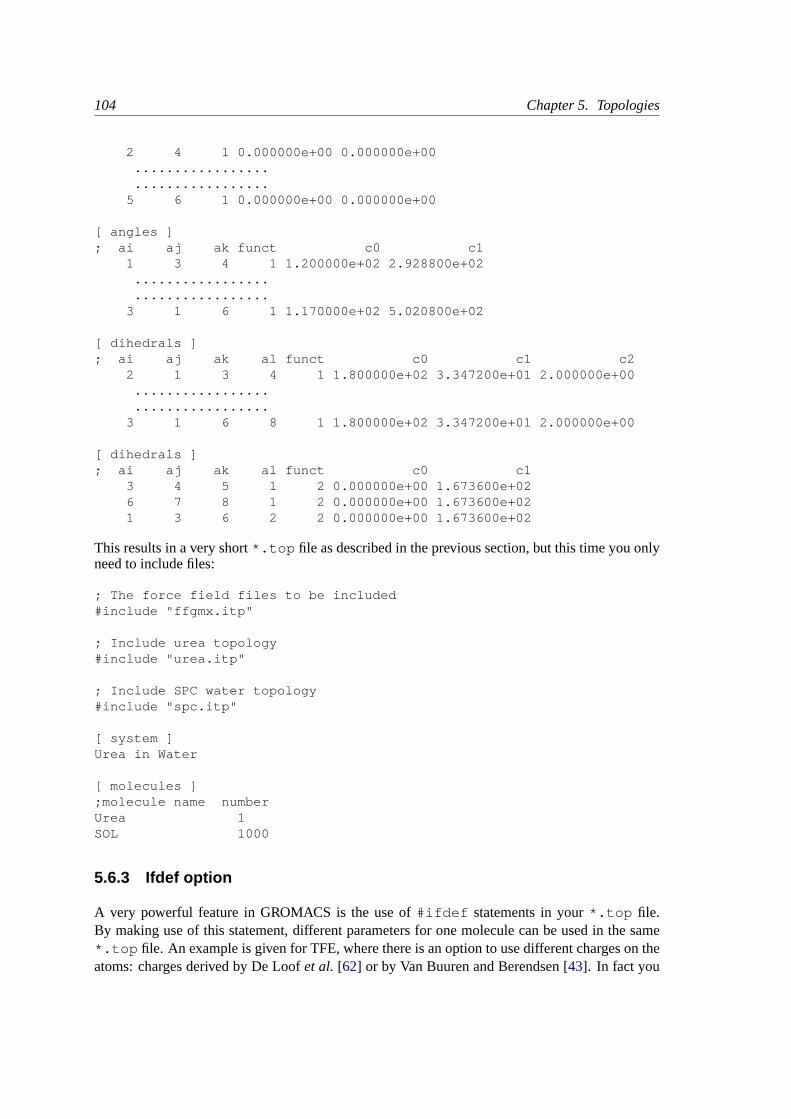
104 Chapter 5. Topologies
2 4 1 0.000000e+00 0.000000e+00..................................
5 6 1 0.000000e+00 0.000000e+00
[ angles ]; ai aj ak funct c0 c1
1 3 4 1 1.200000e+02 2.928800e+02..................................
3 1 6 1 1.170000e+02 5.020800e+02
[ dihedrals ]; ai aj ak al funct c0 c1 c2
2 1 3 4 1 1.800000e+02 3.347200e+01 2.000000e+00..................................
3 1 6 8 1 1.800000e+02 3.347200e+01 2.000000e+00
[ dihedrals ]; ai aj ak al funct c0 c1
3 4 5 1 2 0.000000e+00 1.673600e+026 7 8 1 2 0.000000e+00 1.673600e+021 3 6 2 2 0.000000e+00 1.673600e+02
This results in a very short*.top file as described in the previous section, but this time you onlyneed to include files:
; The force field files to be included#include "ffgmx.itp"
; Include urea topology#include "urea.itp"
; Include SPC water topology#include "spc.itp"
[ system ]Urea in Water
[ molecules ];molecule name numberUrea 1SOL 1000
5.6.3 Ifdef option
A very powerful feature in GROMACS is the use of#ifdef statements in your*.top file.By making use of this statement, different parameters for one molecule can be used in the same*.top file. An example is given for TFE, where there is an option to use different charges on theatoms: charges derived by De Loofet al. [62] or by Van Buuren and Berendsen [43]. In fact you
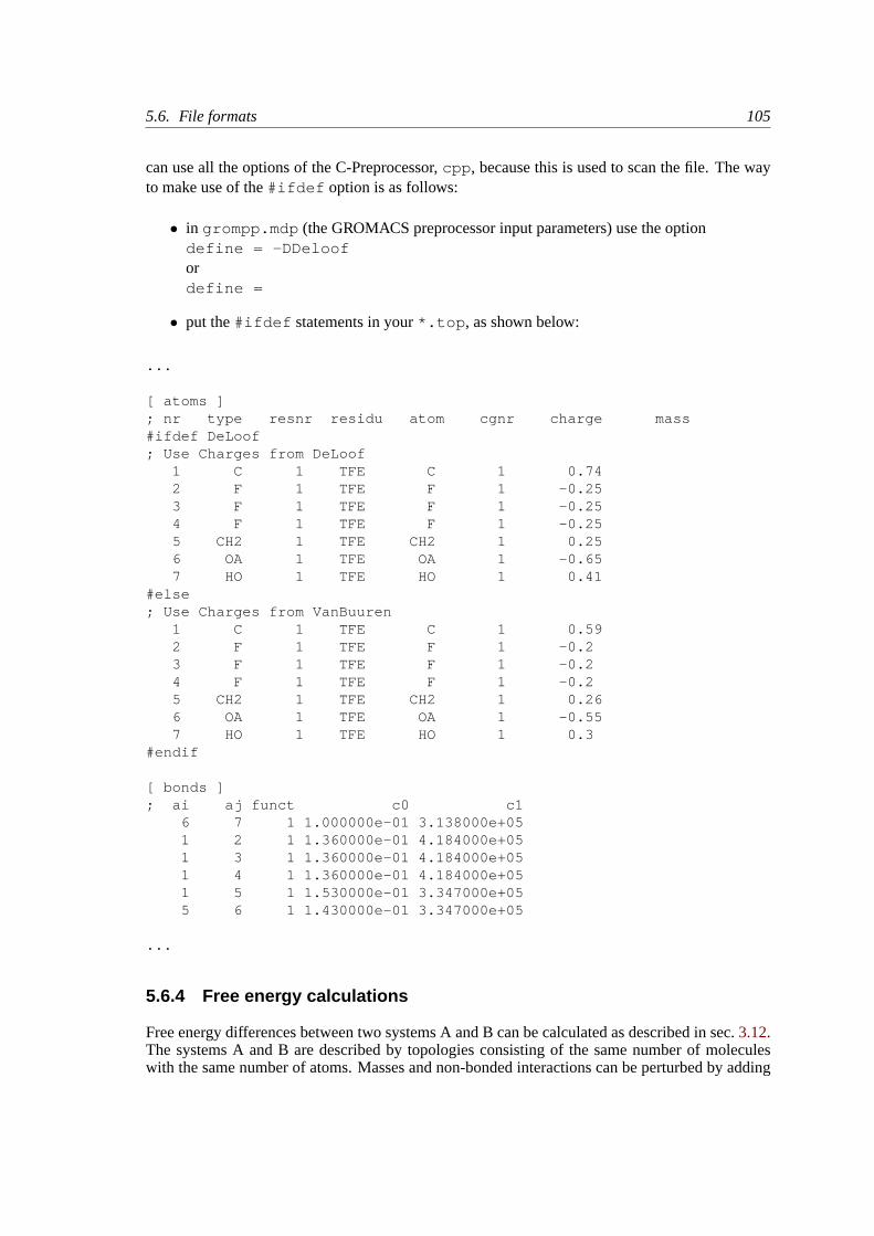
5.6. File formats 105
can use all the options of the C-Preprocessor,cpp , because this is used to scan the file. The wayto make use of the#ifdef option is as follows:
• in grompp.mdp (the GROMACS preprocessor input parameters) use the optiondefine = -DDeloofordefine =
• put the#ifdef statements in your*.top , as shown below:
...
[ atoms ]; nr type resnr residu atom cgnr charge mass#ifdef DeLoof; Use Charges from DeLoof
1 C 1 TFE C 1 0.742 F 1 TFE F 1 -0.253 F 1 TFE F 1 -0.254 F 1 TFE F 1 -0.255 CH2 1 TFE CH2 1 0.256 OA 1 TFE OA 1 -0.657 HO 1 TFE HO 1 0.41
#else; Use Charges from VanBuuren
1 C 1 TFE C 1 0.592 F 1 TFE F 1 -0.23 F 1 TFE F 1 -0.24 F 1 TFE F 1 -0.25 CH2 1 TFE CH2 1 0.266 OA 1 TFE OA 1 -0.557 HO 1 TFE HO 1 0.3
#endif
[ bonds ]; ai aj funct c0 c1
6 7 1 1.000000e-01 3.138000e+051 2 1 1.360000e-01 4.184000e+051 3 1 1.360000e-01 4.184000e+051 4 1 1.360000e-01 4.184000e+051 5 1 1.530000e-01 3.347000e+055 6 1 1.430000e-01 3.347000e+05
...
5.6.4 Free energy calculations
Free energy differences between two systems A and B can be calculated as described in sec.3.12.The systems A and B are described by topologies consisting of the same number of moleculeswith the same number of atoms. Masses and non-bonded interactions can be perturbed by adding
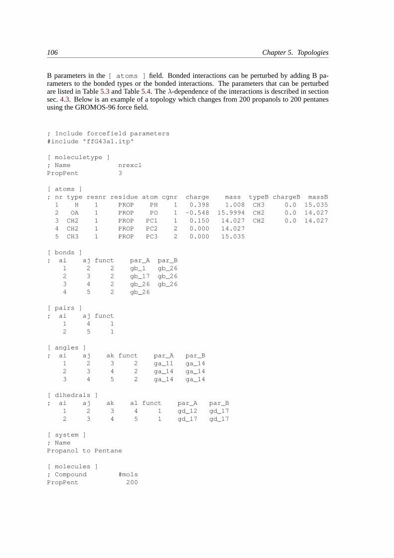
106 Chapter 5. Topologies
B parameters in the[ atoms ] field. Bonded interactions can be perturbed by adding B pa-rameters to the bonded types or the bonded interactions. The parameters that can be perturbedare listed in Table5.3and Table5.4. Theλ-dependence of the interactions is described in sectionsec.4.3. Below is an example of a topology which changes from 200 propanols to 200 pentanesusing the GROMOS-96 force field.
; Include forcefield parameters#include "ffG43a1.itp"
[ moleculetype ]; Name nrexclPropPent 3
[ atoms ]; nr type resnr residue atom cgnr charge mass typeB chargeB massB
1 H 1 PROP PH 1 0.398 1.008 CH3 0.0 15.0352 OA 1 PROP PO 1 -0.548 15.9994 CH2 0.0 14.0273 CH2 1 PROP PC1 1 0.150 14.027 CH2 0.0 14.0274 CH2 1 PROP PC2 2 0.000 14.0275 CH3 1 PROP PC3 2 0.000 15.035
[ bonds ]; ai aj funct par_A par_B
1 2 2 gb_1 gb_262 3 2 gb_17 gb_263 4 2 gb_26 gb_264 5 2 gb_26
[ pairs ]; ai aj funct
1 4 12 5 1
[ angles ]; ai aj ak funct par_A par_B
1 2 3 2 ga_11 ga_142 3 4 2 ga_14 ga_143 4 5 2 ga_14 ga_14
[ dihedrals ]; ai aj ak al funct par_A par_B
1 2 3 4 1 gd_12 gd_172 3 4 5 1 gd_17 gd_17
[ system ]; NamePropanol to Pentane
[ molecules ]; Compound #molsPropPent 200

5.6. File formats 107
Atoms that are not perturbed,PC2 andPC3, do not need B parameter specifications, the B pa-rameters will be copied from the A parameters. Bonded interactions between atoms that are notperturbed do not need B parameter specifications, here this is the case for the last bond. Topolo-gies using the GROMACS force field need no bonded parameters at all, since both the A and Bparameters are determined by the atom types. Non-bonded interactions involving one or two per-turbed atoms use the free-energy perturbation functional forms. Non-bonded interaction betweentwo non-perturbed atoms use the normal functional forms. This means that when, for instance,only the charge of a particle is perturbed, its Lennard-Jones interactions will also be affected whenlambda is not equal to zero or one.
Note that this topology uses the GROMOS-96 force field, in which the bonded interactions are notdetermined by the atom types. The bonded interaction strings are converted by the C-preprocessor.The force field parameter files contain lines like:
#define gb_26 0.1530 7.1500e+06
#define gd_17 0.000 5.86 3
5.6.5 Constraint force
The constraint force between two atoms in one molecule can be calculated with the free energyperturbation code by adding a constraint between the two atoms, with a different length in the Aand B topology. When the B length is 1 nanometer longer than the A length and lambda is keptconstant at zero, the derivative of the Hamiltonian with respect to lambda is the constraint force.For constraints between molecules the pull code can be used, see sec.6.1. Below is an example forcalculating the constraint force at 0.7 nanometer between two methanes in water, by combiningthe two methanes into one molecule. The added constraint is of function type 2, which means thatit is not used for generating exclusions (see5.3.5).
; Include forcefield parameters#include "ffG43a1.itp"
[ moleculetype ]; Name nrexclMethanes 1
[ atoms ]; nr type resnr residu atom cgnr charge mass
1 CH4 1 CH4 C1 1 0 16.0432 CH4 1 CH4 C2 2 0 16.043
[ constraints ]; ai aj funct length_A length_B
1 2 2 0.7 1.7
#include "spc.itp"
[ system ]; NameMethanes in Water

108 Chapter 5. Topologies
[ molecules ]; Compound #molsMethanes 1SOL 2002
5.6.6 Coordinate file
Files with the.gro file extension contain a molecular structure in GROMOS87 format. A samplepiece is included below:
MD of 2 waters, reformat step, PA aug-9161WATER OW1 1 0.126 1.624 1.679 0.1227 -0.0580 0.04341WATER HW2 2 0.190 1.661 1.747 0.8085 0.3191 -0.77911WATER HW3 3 0.177 1.568 1.613 -0.9045 -2.6469 1.31802WATER OW1 4 1.275 0.053 0.622 0.2519 0.3140 -0.17342WATER HW2 5 1.337 0.002 0.680 -1.0641 -1.1349 0.02572WATER HW3 6 1.326 0.120 0.568 1.9427 -0.8216 -0.0244
1.82060 1.82060 1.82060
This format is fixed,i.e. all columns are in a fixed position. If you want to read such a file in yourown program without using the GROMACS libraries you can use the following formats:
C-format: "%5i%5s%5s%5i%8.3f%8.3f%8.3f%8.4f%8.4f%8.4f"
Or to be more precise, with titleetc. it looks like this:
"%s\n", Title"%5d\n", natomsfor (i=0; (i<natoms); i++) {
"%5d%5s%5s%5d%8.3f%8.3f%8.3f%8.4f%8.4f%8.4f\n",residuenr,residuename,atomname,atomnr,x,y,z,vx,vy,vz
}"%10.5f%10.5f%10.5f%10.5f%10.5f%10.5f%10.5f%10.5f%10.5f\n",
box[X][X],box[Y][Y],box[Z][Z],box[X][Y],box[X][Z],box[Y][X],box[Y][Z],box[Z][X],box[Z][Y]
Fortran format: (i5,2a5,i5,3f8.3,3f8.4)
So confin.gro is the GROMACS coordinate file and is almost the same as the GROMOS-87 file (for GROMOS users: when used with ntx=7). The only difference is the box for whichGROMACS uses a tensor, not a vector.
5.7 Force-field organization
5.7.1 Force-field files
GROMACS 3.1.1 includes five forcefields. They are listed the fileFF.dat :
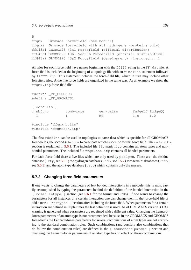
5.7. Force-field organization 109
5ffgmx Gromacs Forcefield (see manual)ffgmx2 Gromacs Forcefield with all hydrogens (proteins only)ffG43a1 GROMOS96 43a1 Forcefield (official distribution)ffG43b1 GROMOS96 43b1 Vacuum Forcefield (official distribution)ffG43a2 GROMOS96 43a2 Forcefield (development) (improved ...)
All files for each force field have names beginning with theff??? string in theFF.dat file. Aforce field is included at the beginning of a topology file with an#include statement followedby ff???.itp . This statement includes the force-field file, which in turn may include otherforcefield files. A the five force fields are organized in the same way. As an example we show theffgmx.itp force-field file:
#define _FF_GROMACS#define _FF_GROMACS1
[ defaults ]; nbfunc comb-rule gen-pairs fudgeLJ fudgeQQ
1 1 no 1.0 1.0
#include "ffgmxnb.itp"#include "ffgmxbon.itp"
The first#define can be used in topologies to parse data which is specific for all GROMACSforce-fields, the second#define to parse data which is specific for this force field. Thedefaultssection is explained in5.6.1. The included fileffgmxnb.itp contains all atom types and non-bonded parameters. The included fileffgmxbon.itp contains all bonded parameters.
For each force field there a five files which are only used bypdb2gmx . These are: the residuedatabase (.rtp , see5.5.1) the hydrogen database (.hdb , see5.5.2), two termini databases (.tdb ,see5.5.3) and the atom type database (.atp ) which contains only the masses.
5.7.2 Changing force-field parameters
If one wants to change the parameters of few bonded interactions in a molcule, this is most eas-ily accomplished by typing the parameters behind the definition of the bonded interaction in the[ moleculetype ] section (see5.6.1for the format and units). If one wants to change theparameters for all instances of a certain interaction one can change them in the force-field file oradd a new[ ???types ] section after including the force field. When parameters for a certaininteraction are defined multiple times the last definition is used. As of GROMACS version 3.1.3 awarning is generated when parameters are redefined with a different value. Changing the Lennard-Jones parameters of an atom type is not recommended, because in the GROMACS and GROMOSforce-fields the Lennard-Jones parameters for several combinations of atom types are not accord-ing to the standard combination rules. Such combinations (and possibly also combinations thatdo follow the combionation rules) are defined in the[ nonbonded params ] section andchanging the Lennard-Jones parameters of an atom type has no effect on these combinations.

110 Chapter 5. Topologies
5.7.3 Adding atom types
As of GROMACS version 3.1.3 atom types can be added in an extra[ atomtypes ] sectionafter the the inclusing of the normal forcefield. After the definition of the new atom type(s), ad-ditional non-bonded and pair parameters can be defined. In pre 3.1.3 versions of GROMACS thenew atom types needed to be added in the[ atomtypes ] section of the forcefield files, be-cause all non-bonded parameters above the last[ atomtypes ] section would be overwrittenusing the standard combination rules.
Chapter 6
Special Topics
6.1 Calculating potentials of mean force: the pull code
There are a number of options to calculate potentials of mean force and related topics. In thecurrent version of GROMACS this is implemented through some extra files formdrun .
6.1.1 Overview
Four different types of calculation are supported:
1. Constraint forcesThe distance between the centers of mass of two groups of atoms can beconstrained and the constraint force monitored. The distance can be in 1, 2, or 3 dimensions.This method uses the SHAKE algorithm but only needs 1 iteration to be exact if only twogroups are constrained.
2. Umbrella sampling A simple umbrella sampling with an harmonic umbrella potential thatacts on the center of mass of a group of atoms.
3. AFM pulling A spring is connected to an atom and slowly retracted. This has the effectof pulling an atom or group of atoms away from its initial location. The rate constant andspring constant for the spring can be varied to study e.g. the unbinding of a protein and aligand (see figure6.1).
4. Starting structures This option creates a number of starting structures for potential of meanforce calculations, moving 1 or 2 groups of atoms at a specified rate towards or away froma reference group, writing out a coordinate file at specified intervals. Note that the groupsgiven in the index file are translated a specified distance each step, but in addition alsoundergo the normal MD, subject to definitions ofe.g. temperature coupling groups, freezegroups and the like.
In the calculations, there has to be 1 reference group and 1 or 2 other groups of atoms. Forconstrained runs, the distance between the reference group and the other groups is kept constant

112 Chapter 6. Special Topics
V
zz link spring
rup
Figure 6.1: Schematic picture of pulling a lipid out of a lipid bilayer with AFM pulling.Vrup isthe velocity at which the spring is retracted,Zlink is the atom to which the spring is attached andZspring is the location of the spring.
at the distance they have in the input coordinate file (.tpr ) file.
6.1.2 Usage
Input files
Themdrun programs needs 4 additional files: 2 input files and 2 output files.
-pi pull.ppaIf this file is specified the pull code will be used. It contains the parameters that control whattype of calculation is done. A full explanation of all the options is given below.
-pn index.ndxThis file defines the different groups for use in all pull calculations. The groups are referredto by name, so the index file can contain other groups that are not used as well.
-po pullout.ppaA formatted copy of the input parameter file with the parameters that were actually used inthe run.
-pdo pull.pdoThe data file with the calculated forces (AFM pulling, constraint force) or positions (um-brella sampling).
Definition of groups
The way the reference groups and different reference types work is summarized in figure6.2.There are four different possibilities for the reference group.
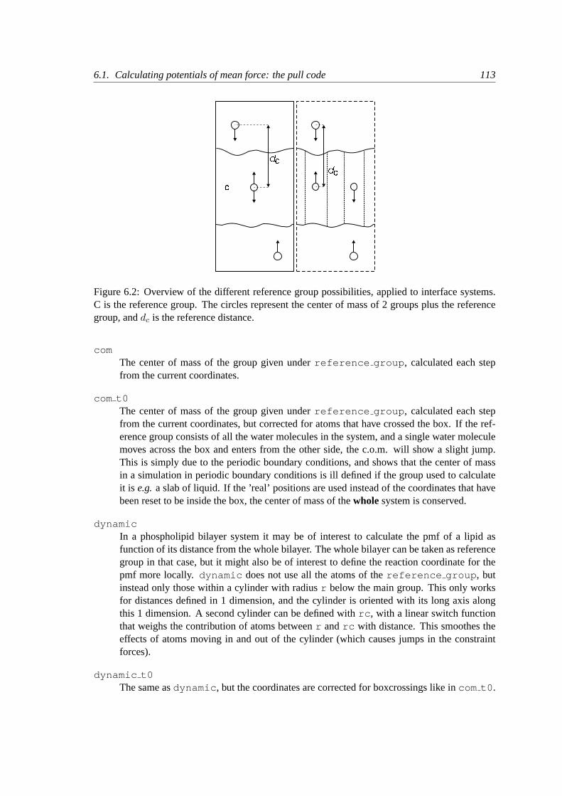
6.1. Calculating potentials of mean force: the pull code 113
�
��
��
Figure 6.2: Overview of the different reference group possibilities, applied to interface systems.C is the reference group. The circles represent the center of mass of 2 groups plus the referencegroup, anddc is the reference distance.
comThe center of mass of the group given underreference group , calculated each stepfrom the current coordinates.
com t0The center of mass of the group given underreference group , calculated each stepfrom the current coordinates, but corrected for atoms that have crossed the box. If the ref-erence group consists of all the water molecules in the system, and a single water moleculemoves across the box and enters from the other side, the c.o.m. will show a slight jump.This is simply due to the periodic boundary conditions, and shows that the center of massin a simulation in periodic boundary conditions is ill defined if the group used to calculateit is e.g.a slab of liquid. If the ’real’ positions are used instead of the coordinates that havebeen reset to be inside the box, the center of mass of thewholesystem is conserved.
dynamicIn a phospholipid bilayer system it may be of interest to calculate the pmf of a lipid asfunction of its distance from the whole bilayer. The whole bilayer can be taken as referencegroup in that case, but it might also be of interest to define the reaction coordinate for thepmf more locally. dynamic does not use all the atoms of thereference group , butinstead only those within a cylinder with radiusr below the main group. This only worksfor distances defined in 1 dimension, and the cylinder is oriented with its long axis alongthis 1 dimension. A second cylinder can be defined withrc , with a linear switch functionthat weighs the contribution of atoms betweenr andrc with distance. This smoothes theeffects of atoms moving in and out of the cylinder (which causes jumps in the constraintforces).
dynamic t0The same asdynamic , but the coordinates are corrected for boxcrossings like incom t0 .
114 Chapter 6. Special Topics
Note that strictly speaking this is not correct if the reference group is not the whole system,including the groups defined withgroup 1 andgroup 2.
To further smooth rapidly fluctuating distances between the reference group and the other groups,the average distance can be constrained instead of the instanteneous distance. This is defined bysettingreflag to the number of steps to average over. However, using this option is not strictlycorrect for calculating potentials of mean force from the average constraint force.
The parameter file
verbose = noIf this is set toyes , a large amount of detailed information is sent tostderr , which isonly useful for diagnostic purposes. The.pdo file also becomes more detailed, which isnot necessary for normal use.
runtype = constraintOptions arestart, afm, constraint, umbrella . This selects the type of cal-culation: making starting structures, AFM pulling, constraint force calculation or umbrellasampling.
group 1 = MB21 1
group 2 = MB21 2The groups with the atoms to act on. The first group is mandatory, the second optional.
reference group = OCTAThe reference group. Distances are calculated betweeengroup 1 (andgroup 2 if spec-ified) and this group. Ife.g. the constraint force between two ions is needed, you wouldspecifiygroup 1 as a group with 1 ion, andreference group as the other ion.
reftype = comThe type of reference group. Options arecom, com t0, dynamic, dynamic t0 asexplained above.
reflag = 1The position of the reference group can be taken as average over a number of steps, specifiedby reflag (see above).
direction = 0.0 0.0 1.0Distances are calculated weighted by x, y, z as specified indirection . Setting them allto 1.0 calculates the distance between two groups, setting the first two to 0.0 and the thirdto 1.0 calculates the distance in the z direction only.
reverse = to referenceThis option selects the direction in which the groups are moved with respect to the referencegroup for AFM pulling and starting structure calculations. Choices areto reference,from reference .
6.1. Calculating potentials of mean force: the pull code 115
r = 0If dynamic reference groups are selected (dynamic, dynamic t0 ), r is the radius ofthe cylinder used to define which atoms are part of the reference group (see above).
rc = 0With dynamic reference groups, the cylinder can be smoothly switched so that atoms thatfall betweenr andrc are weighted linearly from 1 to 0 going fromr to rc . As reasonableinitial values we suggestr = 1.0 andrc = 1.5 , but this will depend strongly on theexact system of interest.
update = 1The frequency with which the dynamic reference groups are recalculated. Usually there isno reason to use anything other than 1.
pullrate = 0.00005The pull rate in nm/timestep for AFM pulling.
forceconstant = 100The force constant for the spring in AFM pulling, in kJ mol−1 nm−2.
width = 0Width of the umbrella sampling potential in kJ mol−1 nm−2.
r0 group2 = 0.0 0.0 3.300The initial location of the groups with respect to the reference group. Only coordinatesselected withdirection are taken into account. The groups are moved to these initialpositions before the actual creation of a series of starting structures commences.
tolerance = 0.001The accuracy with which the actual position of the groups must match the calculated idealpositions for a starting structure (in nm).
translation rate = 0.00001The rate of translation in all directions (nm/step). As mentioned above, normal MD forcecalculations and position updates also act on the groups.
transstep = 0.2The interval in nm at which structures are written out.
6.1.3 Output
The output file is a text file with forces or positions, one per line. If there are two groups theyalternate in the output file. Currently there is no supported analysis program to read this file, but itis simple to parse.
6.1.4 Limitations
Apart from obvious limitations that are simply not implemented (e.g. a better umbrella samplingand analysis scheme), there is one important limitation: constraint forces canonly be calculated
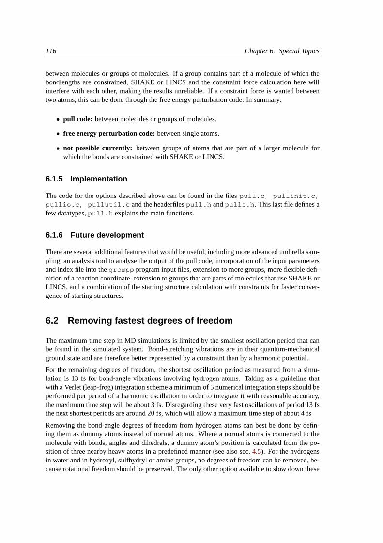
116 Chapter 6. Special Topics
between molecules or groups of molecules. If a group contains part of a molecule of which thebondlengths are constrained, SHAKE or LINCS and the constraint force calculation here willinterfere with each other, making the results unreliable. If a constraint force is wanted betweentwo atoms, this can be done through the free energy perturbation code. In summary:
• pull code: between molecules or groups of molecules.
• free energy perturbation code:between single atoms.
• not possible currently: between groups of atoms that are part of a larger molecule forwhich the bonds are constrained with SHAKE or LINCS.
6.1.5 Implementation
The code for the options described above can be found in the filespull.c, pullinit.c,pullio.c, pullutil.c and the headerfilespull.h andpulls.h . This last file defines afew datatypes,pull.h explains the main functions.
6.1.6 Future development
There are several additional features that would be useful, including more advanced umbrella sam-pling, an analysis tool to analyse the output of the pull code, incorporation of the input parametersand index file into thegrompp program input files, extension to more groups, more flexible defi-nition of a reaction coordinate, extension to groups that are parts of molecules that use SHAKE orLINCS, and a combination of the starting structure calculation with constraints for faster conver-gence of starting structures.
6.2 Removing fastest degrees of freedom
The maximum time step in MD simulations is limited by the smallest oscillation period that canbe found in the simulated system. Bond-stretching vibrations are in their quantum-mechanicalground state and are therefore better represented by a constraint than by a harmonic potential.
For the remaining degrees of freedom, the shortest oscillation period as measured from a simu-lation is 13 fs for bond-angle vibrations involving hydrogen atoms. Taking as a guideline thatwith a Verlet (leap-frog) integration scheme a minimum of 5 numerical integration steps should beperformed per period of a harmonic oscillation in order to integrate it with reasonable accuracy,the maximum time step will be about 3 fs. Disregarding these very fast oscillations of period 13 fsthe next shortest periods are around 20 fs, which will allow a maximum time step of about 4 fs
Removing the bond-angle degrees of freedom from hydrogen atoms can best be done by defin-ing them as dummy atoms instead of normal atoms. Where a normal atoms is connected to themolecule with bonds, angles and dihedrals, a dummy atom’s position is calculated from the po-sition of three nearby heavy atoms in a predefined manner (see also sec.4.5). For the hydrogensin water and in hydroxyl, sulfhydryl or amine groups, no degrees of freedom can be removed, be-cause rotational freedom should be preserved. The only other option available to slow down these
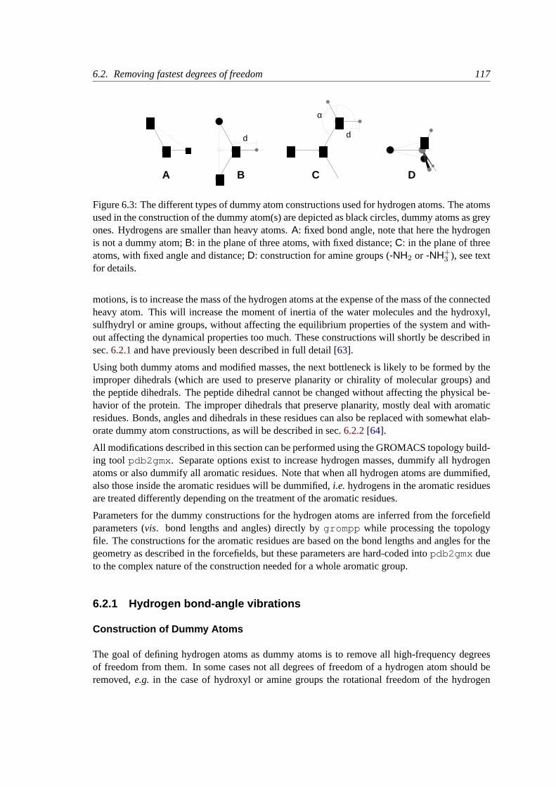
6.2. Removing fastest degrees of freedom 117
D
d
α
d
BA C
�������������������� ����������
������������������������������
��������������������
��������
��������������������
� ���
��������������������
��������������������
Figure 6.3: The different types of dummy atom constructions used for hydrogen atoms. The atomsused in the construction of the dummy atom(s) are depicted as black circles, dummy atoms as greyones. Hydrogens are smaller than heavy atoms.A: fixed bond angle, note that here the hydrogenis not a dummy atom;B: in the plane of three atoms, with fixed distance;C: in the plane of threeatoms, with fixed angle and distance;D: construction for amine groups (-NH2 or -NH+
3 ), see textfor details.
motions, is to increase the mass of the hydrogen atoms at the expense of the mass of the connectedheavy atom. This will increase the moment of inertia of the water molecules and the hydroxyl,sulfhydryl or amine groups, without affecting the equilibrium properties of the system and with-out affecting the dynamical properties too much. These constructions will shortly be described insec.6.2.1and have previously been described in full detail [63].
Using both dummy atoms and modified masses, the next bottleneck is likely to be formed by theimproper dihedrals (which are used to preserve planarity or chirality of molecular groups) andthe peptide dihedrals. The peptide dihedral cannot be changed without affecting the physical be-havior of the protein. The improper dihedrals that preserve planarity, mostly deal with aromaticresidues. Bonds, angles and dihedrals in these residues can also be replaced with somewhat elab-orate dummy atom constructions, as will be described in sec.6.2.2[64].
All modifications described in this section can be performed using the GROMACS topology build-ing tool pdb2gmx . Separate options exist to increase hydrogen masses, dummify all hydrogenatoms or also dummify all aromatic residues. Note that when all hydrogen atoms are dummified,also those inside the aromatic residues will be dummified,i.e. hydrogens in the aromatic residuesare treated differently depending on the treatment of the aromatic residues.
Parameters for the dummy constructions for the hydrogen atoms are inferred from the forcefieldparameters (vis. bond lengths and angles) directly bygrompp while processing the topologyfile. The constructions for the aromatic residues are based on the bond lengths and angles for thegeometry as described in the forcefields, but these parameters are hard-coded intopdb2gmx dueto the complex nature of the construction needed for a whole aromatic group.
6.2.1 Hydrogen bond-angle vibrations
Construction of Dummy Atoms
The goal of defining hydrogen atoms as dummy atoms is to remove all high-frequency degreesof freedom from them. In some cases not all degrees of freedom of a hydrogen atom should beremoved,e.g. in the case of hydroxyl or amine groups the rotational freedom of the hydrogen

118 Chapter 6. Special Topics
atom(s) should be preserved. Care should be taken that no unwanted correlations are introducedby the construction of dummy atoms,e.g.bond-angle vibration between the constructing atomscould translate into hydrogen bond-length vibration. Additionally, since dummy atoms are bydefinition massless, in order to preserve total system mass, the mass of each hydrogen atom thatis treated as dummy atom should be added to the bonded heavy atom.
Taking into account these considerations, the hydrogen atoms in a protein naturally fall into severalcategories, each requiring a different approach (see also Fig.6.3).
• hydroxyl (-OH) or sulfhydryl (-SH) hydrogen: The only internal degree of freedom in ahydroxyl group that can be constrained is the bending of theC-O-H angle. This angle isfixed by defining an additional bond of appropriate length, see Fig.6.3A. This removes thehigh frequency angle bending, but leaves the dihedral rotational freedom. The same goes fora sulfhydryl group. Note that in these cases the hydrogen is not treated as a dummy atom.
• single amine or amide (-NH-) and aromatic hydrogens (-CH-): The position of these hy-drogens cannot be constructed from a linear combination of bond vectors, because of theflexibility of the angle between the heavy atoms. Instead, the hydrogen atom is positionedat a fixed distance from the bonded heavy atom on a line going through the bonded heavyatom and a point on the line through both second bonded atoms, see Fig.6.3B.
• planar amine (-NH2) hydrogens:The method used for the single amide hydrogen is not wellsuited for planar amine groups, because no suitable two heavy atoms can be found to definethe direction of the hydrogen atoms. Instead, the hydrogen is constructed at a fixed distancefrom the nitrogen atom, with a fixed angle to the carbon atom, in the plane defined by oneof the other heavy atoms, see Fig.6.3C.
• amine group (umbrella-NH2 or -NH+3 ) hydrogens:Amine hydrogens with rotational free-
dom cannot be constructed as dummy atoms from the heavy atoms they are connected to,since this would result in loss of the rotational freedom of the amine group. To preservethe rotational freedom while removing the hydrogen bond-angle degrees of freedom, two“dummy masses” are constructed with the same total mass, moment of inertia (for rotationaround theC-N bond) and center of mass as the amine group. These dummy masses haveno interaction with any other atom, except for the fact that they are connected to the carbonand to each other, resulting in a rigid triangle. From these three particles the positions of thenitrogen and hydrogen atoms are constructed as linear combinations of the two carbon-massvectors and their outer product, resulting in an amine group with rotational freedom intact,but without other internal degrees of freedom. See Fig.6.3D.
6.2.2 Out-of-plane vibrations in aromatic groups
The planar arrangements in the side chains of the aromatic residues lends itself perfectly to adummy-atom construction, giving a perfectly planar group without the inherently instable con-straints that are necessary to keep normal atoms in a plane. The basic approach is to define threeatoms or dummy masses with constraints between them to fix the geometry and create the rest ofthe atoms as simple dummy type 3 atoms (see sec.4.5) from these three. Each of the aromaticresidues require a different approach:
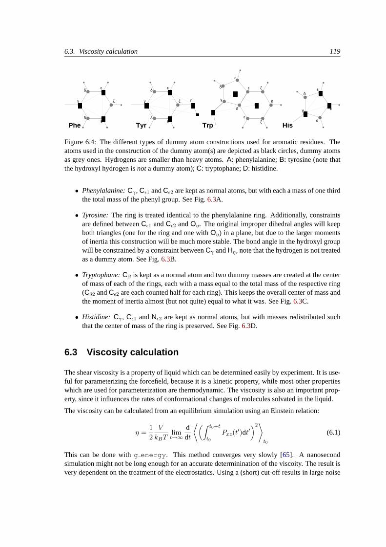
6.3. Viscosity calculation 119
ε
η
ζδ
ε
γ
ε
δ ε
δ
εδ
γ
ζε
η
εδ
γ
Phe Tyr HisTrp
ζ
ε
ζ
εδ
γ
δδ
��������������������
��������������������
��������������������
��������������������
��������
��������������������
� ���
�������������������� ��������������������
��������������������
��������������������
��������������������
����������������������������������������
Figure 6.4: The different types of dummy atom constructions used for aromatic residues. Theatoms used in the construction of the dummy atom(s) are depicted as black circles, dummy atomsas grey ones. Hydrogens are smaller than heavy atoms.A: phenylalanine;B: tyrosine (note thatthe hydroxyl hydrogen isnota dummy atom);C: tryptophane;D: histidine.
• Phenylalanine:Cγ , Cε1 andCε2 are kept as normal atoms, but with each a mass of one thirdthe total mass of the phenyl group. See Fig.6.3A.
• Tyrosine: The ring is treated identical to the phenylalanine ring. Additionally, constraintsare defined betweenCε1 andCε2 andOη. The original improper dihedral angles will keepboth triangles (one for the ring and one withOη) in a plane, but due to the larger momentsof inertia this construction will be much more stable. The bond angle in the hydroxyl groupwill be constrained by a constraint betweenCγ andHη, note that the hydrogen is not treatedas a dummy atom. See Fig.6.3B.
• Tryptophane:Cβ is kept as a normal atom and two dummy masses are created at the centerof mass of each of the rings, each with a mass equal to the total mass of the respective ring(Cδ2 andCε2 are each counted half for each ring). This keeps the overall center of mass andthe moment of inertia almost (but not quite) equal to what it was. See Fig.6.3C.
• Histidine: Cγ , Cε1 andNε2 are kept as normal atoms, but with masses redistributed suchthat the center of mass of the ring is preserved. See Fig.6.3D.
6.3 Viscosity calculation
The shear viscosity is a property of liquid which can be determined easily by experiment. It is use-ful for parameterizing the forcefield, because it is a kinetic property, while most other propertieswhich are used for parameterization are thermodynamic. The viscosity is also an important prop-erty, since it influences the rates of conformational changes of molecules solvated in the liquid.
The viscosity can be calculated from an equilibrium simulation using an Einstein relation:
η =12V
kBTlimt→∞
ddt
⟨(∫ t0+t
t0Pxz(t′)dt′
)2⟩
t0
(6.1)
This can be done withg energy . This method converges very slowly [65]. A nanosecondsimulation might not be long enough for an accurate determinination of the viscoity. The result isvery dependent on the treatment of the electrostatics. Using a (short) cut-off results in large noise
120 Chapter 6. Special Topics
on the off-diagonal pressure elements, which can increase the calculated viscosity by an order ofmagnitude.
GROMACS also has a non-equilibrium method for determining the viscosity [65]. This makes useof the fact that energy, which is fed into system by external forces, is dissipated through viscousfriction. The generated heat is removed by coupling to a heat bath. For a Newtonian liquid addinga small force will result in a velocity gradient according to the following equation:
ax(z) +η
ρ
∂2vx(z)∂z2
= 0 (6.2)
here we have applied an accelerationax(z) in the x-direction, which is a function of thez-coordinate. In GROMACS the acceleration profile is:
ax(z) = A cos(
2πzlz
)(6.3)
wherelz is the height of the box. The generated velocity profile is:
vx(z) = V cos(
2πzlz
)(6.4)
V = Aρ
η
(lz2π
)2
(6.5)
The viscosity can be calculated fromA andV :
η =A
Vρ
(lz2π
)2
(6.6)
In the simulationV is defined as:
V =
N∑i=1
mivi,x2 cos(
2πzlz
)N∑
i=1
mi
(6.7)
The generated velocity profile is not coupled to the heat bath, moreover the velocity profile isexcluded from the kinetic energy. One would likeV to be as large as possible to get good statistics.However the shear rate should not be so high that the system gets too far from equilibrium. Themaximum shear rate occurs where the cosine is zero, the rate being:
shmax = maxz
∣∣∣∣∂vx(z)∂z
∣∣∣∣ = Aρ
η
lz2π
(6.8)
For a simulation with:η = 10−3 [kg m−1 s−1], ρ = 103 [kg m−3] and lz = 2π [nm], shmax =1 [ps nm−1] A. This shear rate should be smaller than one over the longest correlation time in thesystem. For most liquids this will be the rotation correlation time, which is around 10 picoseconds.In this caseA should be smaller than 0.1 [nm ps−2]. When the shear rate is too high, the observedviscosity will be too low. BecauseV is proportional to the square of the box height, the optimal
6.4. Tabulated functions 121
box is elongated in thez-direction. In general a simulation length of 100 picoseconds is enoughto obtain an accurate value for the viscosity.
The heat generated by the viscous friction is removed by coupling to a heat bath. Because thiscoupling is not instantaneous the real temperature of the liquid will be slightly lower than theobserved temperature. Berendsen derived this temperature shift[20], which can be written in termsof the shear rate as:
Ts =η τ
2ρCvsh2max (6.9)
whereτ is the coupling time for the Berendsen thermostat andCv is the heat capacity. Usingthe values of the example above,τ = 10−13 [s] andCv = 2 · 103 [J kg−1 K−1], we get: Ts =25 [K ps−2] sh2
max. When we want the shear rate to be smaller than1/10 [ps−1], Ts is smaller than0.25 [K], which is negligible.
Note that the system has to build up the velocity profile when starting from an equilibrium state.This build-up time is of the order of the correlation time of the liquid.
Two quantities are written to the energy file, along with their averages and fluctuations:V and1/ηas obtained from (6.6).
6.4 Tabulated functions
6.4.1 Cubic splines for potentials
In some of the inner loops of GROMACS lookup tables are used for computation of potential andforces. The tables are interpolated using a cubic spline algorithm. There are separate tables forelectrostatic, dispersion and repulsion interactions, but for the sake of caching performance thesehave been combined into a single array. The cubic spline interpolation looks like this:
y(x) = ηyi + εyi+1 +h2
6
[(η3 − η)y
′′i + (ε3 − ε)y
′′i+1
](6.10)
whereε = 1-η, andyi andy′′i are the tabulated values of a functiony(x) and its second derivative
respectively. Furthermore,
h = xi+1 − xi (6.11)
ε = (x− xi)/h (6.12)
so that0 ≤ ε < 1. eqn.6.10can be rewritten as
y(x) = yi + ε
(yi+1 − yi −
h2
6
(2y
′′i + y
′′i+1
))+ ε2
(h2
2y′′i
)+ ε3
h2
6
(y′′i+1 − y
′′i
)(6.13)
Note that the x-dependence is completely inε. This can abbreviated to
y(x) = yi + εFi + ε2Gi + ε3Hi (6.14)
From this we can calculate the derivative in order to determine the forces:
dy(x)dx
=dy(x)
dεdεdx
= (Fi + 2εGi + 3ε2Hi)/h (6.15)
122 Chapter 6. Special Topics
If we store in the tableyi, Fi, Gi andHi we need a table of length 4n. The number of pointsper nanometer should be on the order of 500 to 1000, for accurate representation (relative error< 10−4 when n = 500 points/nm). The force routines get a scaling factors as a parameter that isequal to the number of points per nm. (Note thath is s−1).
The algorithm goes a little something like this:
1. Calculate distance vector (rij) and distance rij
2. Multiply r ij by s and truncate to an integer valuen0 to get a table index
3. Calculate fractional component (ε = srij − n0) andε2
4. Do the interpolation to calculate the potentialV and the the scalar forcef
5. Calculate the vector forceF by multiplyingf with rij
The tables are stored internally as yi, Fi, Gi, Hi in the order coulomb, dispersion, repulsion. Intotal there are 12 values in each table entry. However, as evident from eqn.6.10, only two values(y andy′′) are necessary to determine each of the repulsion, dispersion and Coulomb potentials;from theseyi, Fi, Gi andHi can be determined. Hence the GROMACS user only has to specifyy andy′′, for each of these, leading to a total of six functions to be specified in the input to themdrun program.
Note that table lookup is significantlyslowerthan computation of the most simple Lennard-Jonesand Coulomb interaction. However, it is much faster than the shifted coulomb function used inconjunction with the PPPM method. Finally it is much easier to modify a table for the potential(and get a graphical representation of it) than to modify the inner loops of the MD program.
6.4.2 User specified potential functions
You can also use your own potential functions without editing the GROMACS code. The potentialfunction should be according to the following equation
V (rij) =qiqj4πε0
f(rij) + C6g(rij) + C12h(rij) (6.16)
with f,g,h user defined functions. Note that if g(r) represents a normal dispersion interaction, g(r)should be< 0. C6, C12 and the charges are read from the topology. Also note that combinationrules are only supported for Lennard Jones and Buckingham, and that your tables should matchthe parameters in the binary topology.
When you add the following lines in your.mdp file:
rlist = 1.0coulombtype = Userrcoulomb = 1.0vdwtype = Userrvdw = 1.0

6.4. Tabulated functions 123
the MD program will read a single file (the name can be changed with option-table ) with sevencolumns of table lookup data in the order: x, f(x), f”(x), g(x), g”(x), h(x), h”(x). The x should runfrom 0 to rc+0.5, with a spacing of 0.002 nm when you run in single precision, or 0.0005 whenyou run in double precision. In this context rc denotes the maximum of the two cut-offsrvdw andrcoulomb (see above). These variables need not be the same (and need not be 1.0 either). Somefunctions used for potentials contain a singularity at x = 0, but since atoms are normally not closerto each other than 0.1 nm, the function value at x = 0 is not important and the tables can be startedat e.g. 0.02 nm. Finally, it is also possible to combine a standard Coulomb with a modified LJpotential (or vice versa). One then specifies e.g. coulombtype = Cut-off or coulombtype = PME,combined with vdwtype = User. The table file must always contain the 7 columns however, andmeaningful data (i.e. not zeroes) must be entered in all columns. A number of pre-built table filescan be found in the GMXLIB directory, for 6-8, 6-9, 6-10, 6-11, 6-12 Lennard Jones potentialscombined with a normal Coulomb.

124 Chapter 6. Special Topics
Chapter 7
Run parameters andPrograms
7.1 Online and html manuals
All the information in this chapter can also be found in HTML format in your GROMACS datadirectory. The path depends on where your files are installed, but the default location is
/usr/local/gromacs/share/html/online.htmlOr, if you installed from Linux packages it can be found as
/usr/local/share/gromacs/html/online.htmlYou can also use the online from our web site,
www.gromacs.org/documentation/reference3.0/online.html
In addition, we install standard UNIX manuals for all the programs. If you have sourced theGMXRCscript in the GROMACS binary directory for your host they should already be present inyour$MANPATH, and you should be able to type e.g.man grompp.
The program manual pages can also be found in AppendixE in this manual.
7.2 File types
Table7.1 lists the file types used by GROMACS along with a short description, and you can finda more detail description for each file in your HTML reference, or in our online version.
GROMACS files written in xdr format can be read on any architecture with GROMACS version1.6 or later if the configuration script found the XDR libraries on your system. They should alwaysbe present on UNIX since they are necessary for NFS support.
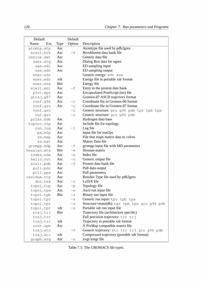
126 Chapter 7. Run parameters and Programs
Default DefaultName Ext. Type Option Description
atomtp.atp Asc Atomtype file used by pdb2gmxeiwit.brk Asc -f Brookhaven data bank file
nnnice.dat Asc Generic data fileuser.dlg Asc Dialog Box data for ngmx
sam.edi Asc ED sampling inputsam.edo Asc ED sampling output
ener.edr Generic energy:edr eneener.edr xdr Energy file in portable xdr formatener.ene Bin Energy file
eiwit.ent Asc -f Entry in the protein date bankplot.eps Asc Encapsulated PostScript (tm) file
gtraj.g87 Asc Gromos-87 ASCII trajectory formatconf.g96 Asc -c Coordinate file in Gromos-96 formatconf.gro Asc -c Coordinate file in Gromos-87 formatconf.gro -c Generic structure:gro g96 pdb tpr tpb tpa
out.gro -o Generic structure:gro g96 pdbpolar.hdb Asc Hydrogen data base
topinc.itp Asc Include file for topologyrun.log Asc -l Log file
ps.m2p Asc Input file for mat2psss.map Asc File that maps matrix data to colorsss.mat Asc Matrix Data file
grompp.mdp Asc -f grompp input file with MD parametershessian.mtx Bin -m Hessian matrix
index.ndx Asc -n Index filehello.out Asc -o Generic output fileeiwit.pdb Asc -f Protein data bank file
pull.pdo Asc Pull data outputpull.ppa Asc Pull parameters
residue.rtp Asc Residue Type file used by pdb2gmxdoc.tex Asc -o LaTeX file
topol.top Asc -p Topology filetopol.tpa Asc -s Ascii run input filetopol.tpb Bin -s Binary run input filetopol.tpr -s Generic run input:tpr tpb tpatopol.tpr -s Structure+mass(db):tpr tpb tpa gro g96 pdbtopol.tpr xdr -s Portable xdr run input file
traj.trj Bin Trajectory file (architecture specific)traj.trr Full precision trajectory:trr trjtraj.trr xdr Trajectory in portable xdr formatroot.xpm Asc X PixMap compatible matrix filetraj.xtc -f Generic trajectory:xtc trr trj gro g96 pdbtraj.xtc xdr Compressed trajectory (portable xdr format)
graph.xvg Asc -o xvgr/xmgr file
Table 7.1: The GROMACS file types.
7.3. Run Parameters 127
7.3 Run Parameters
7.3.1 General
Default values are given in parentheses. The first option is always the default option. Units aregiven in square brackets The difference between a dash and an underscore is ignored. A sample.mdp file is available. This should be appropriate to start a normal simulation. Edit it to suit yourspecific needs and desires.
7.3.2 Preprocessing
title:this is redundant, so you can type anything you want
cpp: (/lib/cpp)your preprocessor
include:directories to include in your topology. Format:-I/home/john/my lib -I../more lib
define: ()defines to pass to the preprocessor, default is no defines. You can use any defines to controloptions in your customized topology files. Options that are already available by default are:
-DFLEX SPCWill tell grompp to include FLEXSPC in stead of SPC into your topology, this is nec-essary to makeconjugate gradientwork and will allowsteepest descentto minimizefurther.
-DPOSREWill tell grompp to include posre.itp into your topology, used for position restraints.
7.3.3 Run control
integrator:
mdA leap-frog algorithm for integrating Newton’s equations of motion.
sdA leap-frog stochastic dynamics integrator. The temperature for one or more groups ofatoms (tc grps) is set withref t [K], the inverse friction constant for each group is setwith tau t [ps]. The parametertcoupl is ignored. The random generator is initializedwith ld seed.NOTE: temperature deviations decay twice as fast as with a Berendsen thermostat withthe sametau t.
128 Chapter 7. Run parameters and Programs
bdAn Euler integrator for Brownian or position Langevin dynamics, the velocity is theforce divided by a friction coefficient (bd fric [amu ps−1]) plus random thermal noise(bd temp [K]). When bd fric =0, the friction coefficient for each particle is calcu-lated as mass/tau t, as for the integratorsd . The random generator is initialized withld seed.
The following algorithms are not integrators, but selected usingthe integrator tag anyway
steepA steepest descent algorithm for energy minimization. The maximum step size isemstep[nm], the tolerance isemtol [kJ mol−1 nm−1].
cgA conjugate gradient algorithm for energy minimization, the tolerance isemtol [kJmol−1 nm−1]. CG is more efficient when a steepest descent step is done every oncein a while, this is determined bynstcgsteep. For a minimization prior to a normalmode analysis, which requires a very high accuracy, GROMACS should be compiledin double precision.
nmNormal mode analysis is performed on the structure in thetpr file. GROMACSshould be compiled in double precision.
tinit: (0) [ps]starting time for your run (only makes sense for integratorsmd, sd andbd)
dt: (0.001) [ps]time step for integration (only makes sense for integratorsmd, sd andbd)
nsteps: (0)maximum number of steps to integrate
comm mode:
LinearRemove center of mass translation
AngularRemove center of mass translation and rotation around the center of mass
NoNo restriction on the center of mass motion
nstcomm: (1) [steps]frequency for center of mass motion removal
comm grps:group(s) for center of mass motion removal, default is the whole system
7.3. Run Parameters 129
7.3.4 Langevin dynamics
bd temp: (300) [K]temperature in Brownian dynamics run (controls thermal noise level). Whenbd fric =0,ref t is used instead.
bd fric: (0) [amu ps−1]Brownian dynamics friction coefficient. Whenbd fric =0, the friction coefficient for eachparticle is calculated as mass/tau t.
ld seed: (1993) [integer]used to initialize random generator for thermal noise for stochastic and Brownian dynam-ics. Whenld seedis set to -1, the seed is calculated as(time() + getpid()) %1000000 . When running on multiple processors, each processor uses a seed equal told seedplus the processor number.
7.3.5 Energy minimization
emtol: (100.0) [kJ mol−1 nm−1]the minimization is converged when the maximum force is smaller than this value
emstep: (0.01) [nm]initial step-size
nstcgsteep: (1000) [steps]frequency of performing 1 steepest descent step while doing conjugate gradient energy min-imization.
7.3.6 Shell Molecular Dynamics
When doing shell molecular dynamics the positions of the shells are optimized at every time stepuntil either the RMS force on the shells is less than emtol, or a maximum number of iterations(niter) has been reached
emtol: (100.0) [kJ mol−1 nm−1]the minimization is converged when the maximum force is smaller than this value. For shellMD this value should be 1.0 at most, but since the variable is used for energy minimizationas well the default is 100.0.
niter: (20)maximum number of iterations for optimizing the shell positions.
7.3.7 Output control
nstxout: (100) [steps]frequency to write coordinates to output trajectory file, the last coordinates are always writ-ten
130 Chapter 7. Run parameters and Programs
nstvout: (100) [steps]frequency to write velocities to output trajectory, the last velocities are always written
nstfout: (0) [steps]frequency to write forces to output trajectory.
nstlog: (100) [steps]frequency to write energies to log file, the last energies are always written
nstenergy: (100) [steps]frequency to write energies to energy file, the last energies are always written
nstxtcout: (0) [steps]frequency to write coordinates to xtc trajectory
xtc precision: (1000) [real]precision to write to xtc trajectory
xtc grps:group(s) to write to xtc trajectory, default the whole system is written (ifnstxtcout is largerthan zero)
energygrps:group(s) to write to energy file
7.3.8 Neighbor searching
nstlist: (10) [steps]Frequency to update the neighbor list (and the long-range forces, when using twin-rangecut-off’s). When this is 0, the neighbor list is made only once.
ns type:
gridMake a grid in the box and only check atoms in neighboring grid cells when construct-ing a new neighbor list everynstlist steps. In large systems grid search is much fasterthan simple search.
simpleCheck every atom in the box when constructing a new neighbor list everynstlist steps.
pbc:
xyzUse periodic boundary conditions in all directions.
noUse no periodic boundary conditions, ignore the box. To simulate without cut-offs, setall cut-offs to 0 andnstlist=0.
rlist: (1) [nm]cut-off distance for the short-range neighbor list

7.3. Run Parameters 131
7.3.9 Electrostatics and VdW
coulombtype:
Cut-offTwin range cut-off’s with neighborlist cut-offrlist and Coulomb cut-offrcoulomb,whererlist < rvdw < rcoulomb. The dielectric constant is set withepsilon r .
EwaldClassical Ewald sum electrostatics. Usee.g.rlist =0.9,rvdw=0.9,rcoulomb=0.9. Thehighest magnitude of wave vectors used in reciprocal space is controlled byfouri-erspacing. The relative accuracy of direct/reciprocal space is controlled byewald rtol .NOTE: Ewald scales as O(N3/2) and is thus extremely slow for large systems. It isincluded mainly for reference - in most cases PME will perform much better.
PMEFast Particle-Mesh Ewald electrostatics. Direct space is similar to the Ewald sum,while the reciprocal part is performed with FFTs. Grid dimensions are controlled withfourierspacing and the interpolation order withpme order. With a grid spacing of0.1 nm and cubic interpolation the electrostatic forces have an accuracy of 2-3e-4.Since the error from the vdw-cutoff is larger than this you might try 0.15 nm. Whenrunning in parallel the interpolation parallelizes better than the FFT, so try decreasinggrid dimensions while increasing interpolation.
PPPMParticle-Particle Particle-Mesh algorithm for long range electrostatic interactions. Usefor examplerlist =1.0 , rcoulomb switch=0.0 , rcoulomb=0.85 , rvdw switch=1.0andrvdw=1.0 . The grid dimensions are controlled byfourierspacing. Reasonablegrid spacing for PPPM is 0.05-0.1 nm. SeeShift for the details of the particle-particle potential.
NOTE: the pressure in incorrect when using PPPM.
Reaction-FieldReaction field with Coulomb cut-offrcoulomb, wherercoulomb> rvdw > rlist . Thedielectric constant beyond the cut-off isepsilon r . The dielectric constant can be setto infinity by settingepsilon r=0.
Generalized-Reaction-FieldGeneralized reaction field with Coulomb cut-offrcoulomb, wherercoulomb > rvdw> rlist . The dielectric constant beyond the cut-off isepsilon r . The ionic strength iscomputed from the number of charged (i.e. with non zero charge) charge groups. Thetemperature for the GRF potential is set withref t [K].
ShiftThe Coulomb potential is decreased over the whole range and the forces decay smoothlyto zero betweenrcoulomb switch andrcoulomb. The neighbor search cut-offrlistshould be 0.1 to 0.3 nm larger thanrcoulomb to accommodate for the size of chargegroups and diffusion between neighbor list updates.
UserSpecify rlist and rcoulomb to the same value,mdrun will now expect to find a
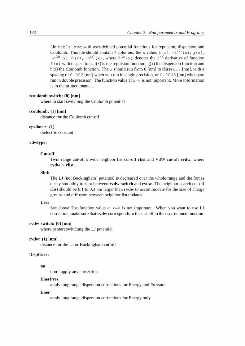
132 Chapter 7. Run parameters and Programs
file table.xvg with user-defined potential functions for repulsion, dispersion andCoulomb. This file should contain 7 columns: thex value,f(x) , -f (2)(x) , g(x) ,-g (2)(x) , h(x) , -h (2)(x) , wheref (2)(x) denotes the2nd derivative of functionf(x) with respect tox . f(x) is the repulsion function, g(x) the dispersion function andh(x) the Coulomb function. Thex should run from 0 [nm] torlist +0.5 [nm], with aspacing of0.002 [nm] when you run in single precision, or0.0005 [nm] when yourun in double precision. The function value atx=0 is not important. More informationis in the printed manual.
rcoulomb switch: (0) [nm]where to start switching the Coulomb potential
rcoulomb: (1) [nm]distance for the Coulomb cut-off
epsilon r: (1)dielectric constant
vdwtype:
Cut-offTwin range cut-off’s with neighbor list cut-offrlist and VdW cut-offrvdw , wherervdw > rlist .
ShiftThe LJ (not Buckingham) potential is decreased over the whole range and the forcesdecay smoothly to zero betweenrvdw switch andrvdw . The neighbor search cut-offrlist should be 0.1 to 0.3 nm larger thanrvdw to accommodate for the size of chargegroups and diffusion between neighbor list updates.
UserSee above The function value atx=0 is not important. When you want to use LJcorrection, make sure thatrvdw corresponds to the cut-off in the user-defined function.
rvdw switch: (0) [nm]where to start switching the LJ potential
rvdw: (1) [nm]distance for the LJ or Buckingham cut-off
DispCorr:
nodon’t apply any correction
EnerPresapply long range dispersion corrections for Energy and Pressure
Enerapply long range dispersion corrections for Energy only
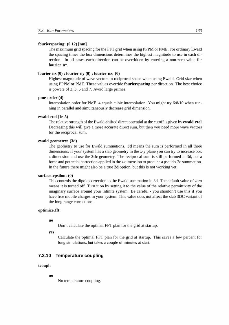
7.3. Run Parameters 133
fourierspacing: (0.12) [nm]The maximum grid spacing for the FFT grid when using PPPM or PME. For ordinary Ewaldthe spacing times the box dimensions determines the highest magnitude to use in each di-rection. In all cases each direction can be overridden by entering a non-zero value forfourier n* .
fourier nx (0) ; fourier ny (0) ; fourier nz: (0)Highest magnitude of wave vectors in reciprocal space when using Ewald. Grid size whenusing PPPM or PME. These values overridefourierspacing per direction. The best choiceis powers of 2, 3, 5 and 7. Avoid large primes.
pme order (4)Interpolation order for PME. 4 equals cubic interpolation. You might try 6/8/10 when run-ning in parallel and simultaneously decrease grid dimension.
ewald rtol (1e-5)The relative strength of the Ewald-shifted direct potential at the cutoff is given byewald rtol .Decreasing this will give a more accurate direct sum, but then you need more wave vectorsfor the reciprocal sum.
ewald geometry: (3d)The geometry to use for Ewald summations.3d means the sum is performed in all threedimensions. If your system has a slab geometry in the x-y plane you can try to increase boxz dimension and use the3dc geometry. The reciprocal sum is still performed in 3d, but aforce and potential correction applied in the z dimension to produce a pseudo-2d summation.In the future there might also be a true2d option, but this is not working yet.
surface epsilon: (0)This controls the dipole correction to the Ewald summation in 3d. The default value of zeromeans it is turned off. Turn it on by setting it to the value of the relative permittivity of theimaginary surface around your infinite system. Be careful - you shouldn’t use this if youhave free mobile charges in your system. This value does not affect the slab 3DC variant ofthe long range corrections.
optimize fft:
noDon’t calculate the optimal FFT plan for the grid at startup.
yesCalculate the optimal FFT plan for the grid at startup. This saves a few percent forlong simulations, but takes a couple of minutes at start.
7.3.10 Temperature coupling
tcoupl:
noNo temperature coupling.
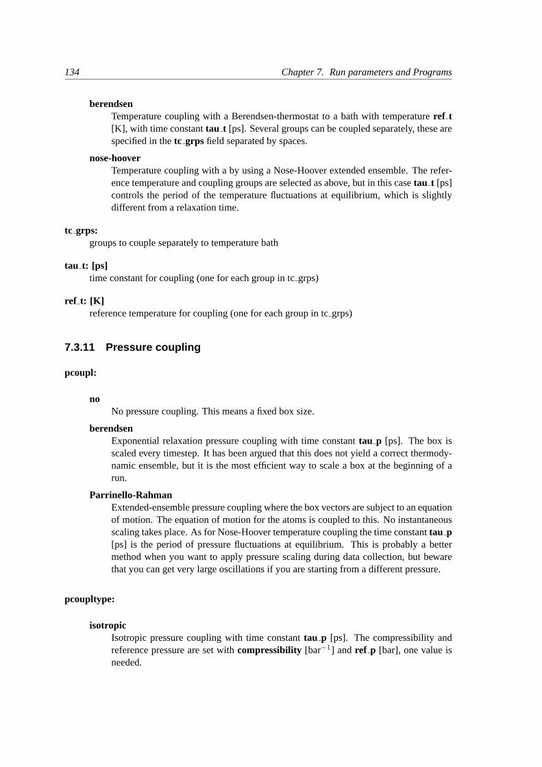
134 Chapter 7. Run parameters and Programs
berendsenTemperature coupling with a Berendsen-thermostat to a bath with temperatureref t[K], with time constanttau t [ps]. Several groups can be coupled separately, these arespecified in thetc grps field separated by spaces.
nose-hooverTemperature coupling with a by using a Nose-Hoover extended ensemble. The refer-ence temperature and coupling groups are selected as above, but in this casetau t [ps]controls the period of the temperature fluctuations at equilibrium, which is slightlydifferent from a relaxation time.
tc grps:groups to couple separately to temperature bath
tau t: [ps]time constant for coupling (one for each group in tcgrps)
ref t: [K]reference temperature for coupling (one for each group in tcgrps)
7.3.11 Pressure coupling
pcoupl:
noNo pressure coupling. This means a fixed box size.
berendsenExponential relaxation pressure coupling with time constanttau p [ps]. The box isscaled every timestep. It has been argued that this does not yield a correct thermody-namic ensemble, but it is the most efficient way to scale a box at the beginning of arun.
Parrinello-RahmanExtended-ensemble pressure coupling where the box vectors are subject to an equationof motion. The equation of motion for the atoms is coupled to this. No instantaneousscaling takes place. As for Nose-Hoover temperature coupling the time constanttau p[ps] is the period of pressure fluctuations at equilibrium. This is probably a bettermethod when you want to apply pressure scaling during data collection, but bewarethat you can get very large oscillations if you are starting from a different pressure.
pcoupltype:
isotropicIsotropic pressure coupling with time constanttau p [ps]. The compressibility andreference pressure are set withcompressibility [bar−1] and ref p [bar], one value isneeded.
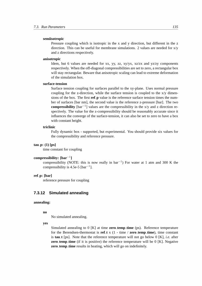
7.3. Run Parameters 135
semiisotropicPressure coupling which is isotropic in the x and y direction, but different in the zdirection. This can be useful for membrane simulations. 2 values are needed for x/yand z directions respectively.
anisotropicIdem, but 6 values are needed for xx, yy, zz, xy/yx, xz/zx and yz/zy componentsrespectively. When the off-diagonal compressibilities are set to zero, a rectangular boxwill stay rectangular. Beware that anisotropic scaling can lead to extreme deformationof the simulation box.
surface-tensionSurface tension coupling for surfaces parallel to the xy-plane. Uses normal pressurecoupling for the z-direction, while the surface tension is coupled to the x/y dimen-sions of the box. The firstref p value is the reference surface tension times the num-ber of surfaces [bar nm], the second value is the reference z-pressure [bar]. The twocompressibility [bar−1] values are the compressibility in the x/y and z direction re-spectively. The value for the z-compressibility should be reasonably accurate since itinfluences the converge of the surface-tension, it can also be set to zero to have a boxwith constant height.
triclinicFully dynamic box - supported, but experimental. You should provide six values forthe compressibility and reference pressure.
tau p: (1) [ps]time constant for coupling
compressibility: [bar−1]compressibility (NOTE: this is now really in bar−1) For water at 1 atm and 300 K thecompressibility is 4.5e-5 [bar−1].
ref p: [bar]reference pressure for coupling
7.3.12 Simulated annealing
annealing:
noNo simulated annealing.
yesSimulated annealing to 0 [K] at timezero temp time (ps). Reference temperaturefor the Berendsen-thermostat isref t x (1 - time / zero temp time), time constantis tau t [ps]. Note that the reference temperature will not go below 0 [K],i.e. afterzero temp time (if it is positive) the reference temperature will be 0 [K]. Negativezero temp time results in heating, which will go on indefinitely.
136 Chapter 7. Run parameters and Programs
zero temp time: (0) [ps]time at which temperature will be zero (can be negative). Temperature during the run can beseen as a straight line going through T=ref t [K] at t=0 [ps], and T=0 [K] at t=zero temp time[ps]. Look in our FAQ for a schematic graph of temperature versus time.
7.3.13 Velocity generation
gen vel:
noDo not generate velocities at startup. The velocities are set to zero when there are novelocities in the input structure file.
yesGenerate velocities according to a Maxwell distribution at temperaturegen temp [K],with random seedgen seed. This is only meaningful with integratormd.
gen temp: (300) [K]temperature for Maxwell distribution
gen seed: (173529) [integer]used to initialize random generator for random velocities, whengen seedis set to -1, theseed is calculated as(time() + getpid()) % 1000000
7.3.14 Bonds
constraints:
noneNo constraints,i.e.bonds are represented by a harmonic or a Morse potential (depend-ing on the setting ofmorse) and angles by a harmonic potential.
hbondsOnly constrain the bonds with H-atoms.
all-bondsConstrain all bonds.
h-anglesConstrain all bonds and constrain the angles that involve H-atoms by adding bond-constraints.
all-anglesConstrain all bonds and constrain all angles by adding bond-constraints.
constraint algorithm:
lincsLINear Constraint Solver. The accuracy in set withlincs order, which sets the numberof matrices in the expansion for the matrix inversion, 4 is enough for a ”normal” MD
7.3. Run Parameters 137
simulation, 8 is needed for BD with large time-steps. The accuracy of the constraints isprinted to the log file everynstlogsteps. If a bond rotates more thanlincs warnangle[degrees] in one step, a warning will be printed both to the log file and tostderr .Lincs should not be used with coupled angle constraints.
shakeShake is slower and less stable than Lincs, but does work with angle constraints. Therelative tolerance is set withshake tol, 0.0001 is a good value for ”normal” MD.
unconstrained start:
noapply constraints to the start configuration
yesdo not apply constraints to the start configuration
shake tol: (0.0001)relative tolerance for shake
lincs order: (4)Highest order in the expansion of the constraint coupling matrix.lincs order is also usedfor the number of Lincs iterations during energy minimization, only one iteration is used inMD.
lincs warnangle: (30) [degrees]maximum angle that a bond can rotate before Lincs will complain
morse:
nobonds are represented by a harmonic potential
yesbonds are represented by a Morse potential
7.3.15 Energy group exclusions
energygrp excl:Pairs of energy groups for which all non-bonded interactions are excluded. An example: ifyou have two energy groupsProtein andSOL, specifying
energy excl = Protein Protein SOL SOL
would give only the non-bonded interactions between the protein and the solvent. This isespecially useful for speeding up energy calculations withmdrun -rerun and for exclud-ing interactions within frozen groups.
138 Chapter 7. Run parameters and Programs
7.3.16 NMR refinement
disre:
nono distance restraints (ignore distance restraint information in topology file)
simplesimple (per-molecule) distance restraints, ensemble averaging can be performed withmdrun -multi
ensembledistance restraints over an ensemble of molecules in one simulation box, should onlybe used for special cases, such as dimers
disre weighting:
conservativethe forces are the derivative of the restraint potential, this results in an r−7 weightingof the atom pairs
equaldivide the restraint force equally over all atom pairs in the restraint
disre mixed:
nothe violation used in the calculation of the restraint force is the time averaged violation
yesthe violation used in the calculation of the restraint force is the square root of the timeaveraged violation times the instantaneous violation
disre fc: (1000) [kJ mol−1 nm−2]force constant for distance restraints, which is multiplied by a (possibly) different factor foreach restraint
disre tau: (0) [ps]time constant for distance restraints running average
nstdisreout: (100) [steps]frequency to write the running time averaged and instantaneous distances of all atom pairsinvolved in restraints to the energy file (can make the energy file very large)
orire:
nono orientation restraints (ignore orientation restraint information in topology file)
yesuse orientation restraints, ensemble averaging can be performed withmdrun -multi
7.3. Run Parameters 139
orire fc: (0) [kJ mol]force constant for orientation restraints, which is multiplied by a (possibly) different factorfor each restraint, can be set to zero to obtain the orientations from a free simulation
orire tau: (0) [ps]time constant for orientation restraints running average
orire fitgrp:fit group for orientation restraining, for a protein backbone is a good choice
nstorireout: (100) [steps]frequency to write the running time averaged orientations for all restraints to the energy file(can make the energy file very large)
7.3.17 Free Energy Perturbation
free energy:
noOnly use topology A.
yesInterpolate between topology A (lambda=0) to topology B (lambda=1) and write thederivative of the Hamiltonian with respect to lambda to the energy file and todgdl.xvg .The potentials, bond-lengths and angles are interpolated linearly as described in themanual. Whensc alpha is larger than zero, soft-core potentials are used for the LJand Coulomb interactions.
init lambda: (0)starting value for lambda
delta lambda: (0)increment per time step for lambda
sc alpha: (0)the soft-core parameter, a value of 0 results in linear interpolation of the LJ and Coulombinteractions
sc sigma: (0.3) [nm]the soft-core sigma for particles which have a C6 or C12 parameter equal to zero
7.3.18 Non-equilibrium MD
acc grps:groups for constant acceleration (e.g.: Protein Sol ) all atoms in groups Protein and Solwill experience constant acceleration as specified in theaccelerateline
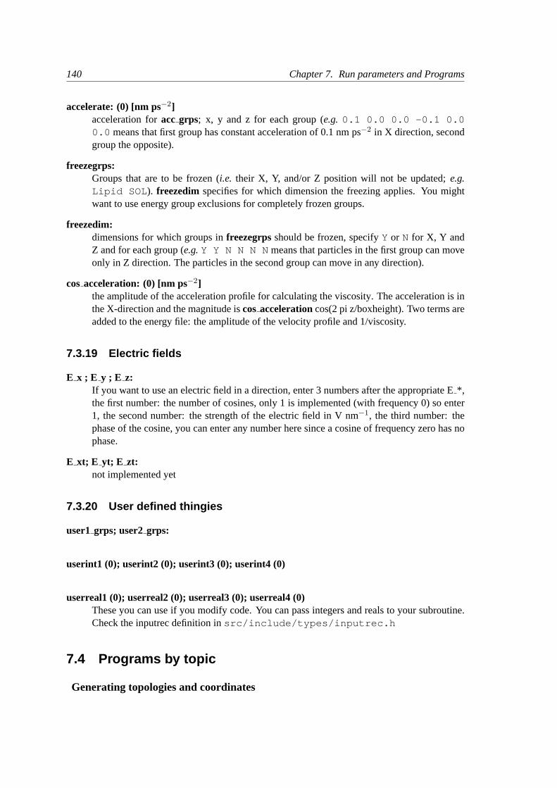
140 Chapter 7. Run parameters and Programs
accelerate: (0) [nm ps−2]acceleration foracc grps; x, y and z for each group (e.g. 0.1 0.0 0.0 -0.1 0.00.0 means that first group has constant acceleration of 0.1 nm ps−2 in X direction, secondgroup the opposite).
freezegrps:Groups that are to be frozen (i.e. their X, Y, and/or Z position will not be updated;e.g.Lipid SOL ). freezedim specifies for which dimension the freezing applies. You mightwant to use energy group exclusions for completely frozen groups.
freezedim:dimensions for which groups infreezegrpsshould be frozen, specifyY or N for X, Y andZ and for each group (e.g.Y Y N N N Nmeans that particles in the first group can moveonly in Z direction. The particles in the second group can move in any direction).
cosacceleration: (0) [nm ps−2]the amplitude of the acceleration profile for calculating the viscosity. The acceleration is inthe X-direction and the magnitude iscosaccelerationcos(2 pi z/boxheight). Two terms areadded to the energy file: the amplitude of the velocity profile and 1/viscosity.
7.3.19 Electric fields
E x ; E y ; E z:If you want to use an electric field in a direction, enter 3 numbers after the appropriate E*,the first number: the number of cosines, only 1 is implemented (with frequency 0) so enter1, the second number: the strength of the electric field in V nm−1, the third number: thephase of the cosine, you can enter any number here since a cosine of frequency zero has nophase.
E xt; E yt; E zt:not implemented yet
7.3.20 User defined thingies
user1 grps; user2 grps:
userint1 (0); userint2 (0); userint3 (0); userint4 (0)
userreal1 (0); userreal2 (0); userreal3 (0); userreal4 (0)These you can use if you modify code. You can pass integers and reals to your subroutine.Check the inputrec definition insrc/include/types/inputrec.h
7.4 Programs by topic
Generating topologies and coordinates
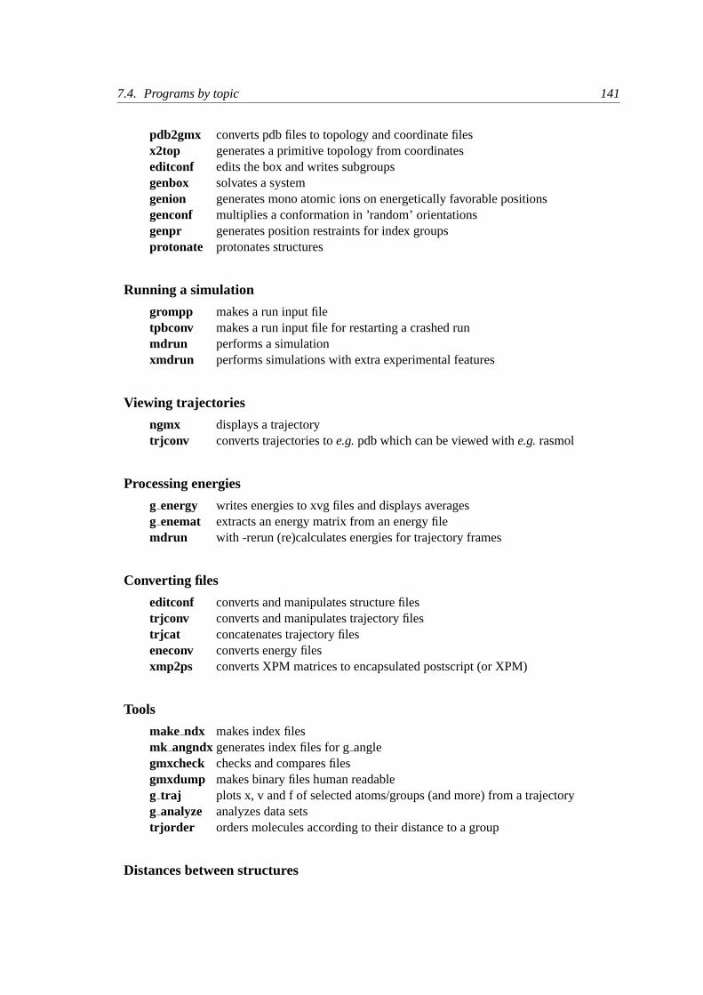
7.4. Programs by topic 141
pdb2gmx converts pdb files to topology and coordinate filesx2top generates a primitive topology from coordinateseditconf edits the box and writes subgroupsgenbox solvates a systemgenion generates mono atomic ions on energetically favorable positionsgenconf multiplies a conformation in ’random’ orientationsgenpr generates position restraints for index groupsprotonate protonates structures
Running a simulation
grompp makes a run input filetpbconv makes a run input file for restarting a crashed runmdrun performs a simulationxmdrun performs simulations with extra experimental features
Viewing trajectories
ngmx displays a trajectorytrjconv converts trajectories toe.g.pdb which can be viewed withe.g.rasmol
Processing energies
g energy writes energies to xvg files and displays averagesg enemat extracts an energy matrix from an energy filemdrun with -rerun (re)calculates energies for trajectory frames
Converting files
editconf converts and manipulates structure filestrjconv converts and manipulates trajectory filestrjcat concatenates trajectory fileseneconv converts energy filesxmp2ps converts XPM matrices to encapsulated postscript (or XPM)
Tools
make ndx makes index filesmk angndxgenerates index files for ganglegmxcheck checks and compares filesgmxdump makes binary files human readableg traj plots x, v and f of selected atoms/groups (and more) from a trajectoryg analyze analyzes data setstrjorder orders molecules according to their distance to a group
Distances between structures
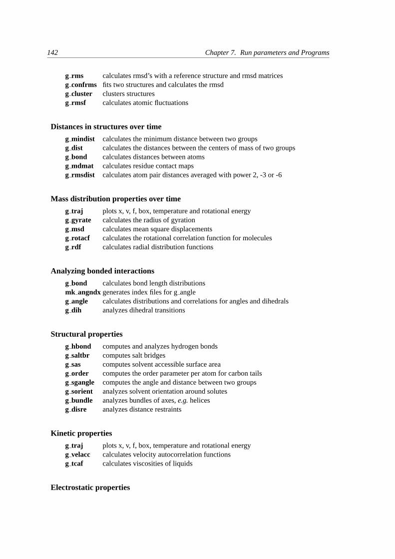
142 Chapter 7. Run parameters and Programs
g rms calculates rmsd’s with a reference structure and rmsd matricesg confrms fits two structures and calculates the rmsdg cluster clusters structuresg rmsf calculates atomic fluctuations
Distances in structures over time
g mindist calculates the minimum distance between two groupsg dist calculates the distances between the centers of mass of two groupsg bond calculates distances between atomsg mdmat calculates residue contact mapsg rmsdist calculates atom pair distances averaged with power 2, -3 or -6
Mass distribution properties over time
g traj plots x, v, f, box, temperature and rotational energyg gyrate calculates the radius of gyrationg msd calculates mean square displacementsg rotacf calculates the rotational correlation function for moleculesg rdf calculates radial distribution functions
Analyzing bonded interactions
g bond calculates bond length distributionsmk angndxgenerates index files for gangleg angle calculates distributions and correlations for angles and dihedralsg dih analyzes dihedral transitions
Structural properties
g hbond computes and analyzes hydrogen bondsg saltbr computes salt bridgesg sas computes solvent accessible surface areag order computes the order parameter per atom for carbon tailsg sgangle computes the angle and distance between two groupsg sorient analyzes solvent orientation around solutesg bundle analyzes bundles of axes,e.g.helicesg disre analyzes distance restraints
Kinetic properties
g traj plots x, v, f, box, temperature and rotational energyg velacc calculates velocity autocorrelation functionsg tcaf calculates viscosities of liquids
Electrostatic properties

7.4. Programs by topic 143
genion generates mono atomic ions on energetically favorable positionsg potential calculates the electrostatic potential across the boxg dipoles computes the total dipole plus fluctuationsg dielectric calculates frequency dependent dielectric constants
Protein specific analysisdo dssp assigns secondary structure and calculates solvent accessible surface areag chi calculates everything you want to know about chi and other dihedralsg helix calculates everything you want to know about helicesg rama computes Ramachandran plotsxrama shows animated Ramachandran plotswheel plots helical wheels
Interfacesg potential calculates the electrostatic potential across the boxg density calculates the density of the systemg order computes the order parameter per atom for carbon tailsg h2order computes the orientation of water moleculesg bundle analyzes bundles of axes,e.g.transmembrane helices
Covariance analysisg covar calculates and diagonalizes the covariance matrixg anaeig analyzes the eigenvectors
Normal modesgrompp makes a run input filemdrun finds a potential energy minimumnmrun calculates the Hessiang nmeig diagonalizes the Hessiang anaeig analyzes the normal modesg nmens generates an ensemble of structures from the normal modes

144 Chapter 7. Run parameters and Programs

Chapter 8
Analysis
In this chapter different ways of analyzing your trajectory are described. The names of the corre-sponding analysis programs are given. Specific info on the in- and output of these programs can befound in the on-line manual atwww.gromacs.org. The output files are often produced as finishedGrace/Xmgr graphs.
First in sec.8.1 the group concept in analysis is explained. Then the different analysis tools arepresented.
8.1 Groups in Analysis.
make_ndxmk_angndx
In chapter3 it was explained howgroups of atomscan be used in the MD-program. In mostanalysis programs groups of atoms are needed to work on. Most programs can generate severaldefault index groups, but groups can always be read from an index file. Let’s consider a simulationof a binary mixture of components A and B. When we want to calculate the radial distributionfunction (rdf)gAB(r) of A with respect to B, we have to calculate
4πr2gAB(r) = VNA∑i∈A
NB∑j∈B
P (r) (8.1)
whereV is the volume andP (r) is the probability to find a B atom at a distancer from an A atom.
By having the user define theatom numbersfor groups A and B in a simple file we can calculatethis gAB in the most general way, without having to make any assumptions in the rdf-programabout the type of particles.
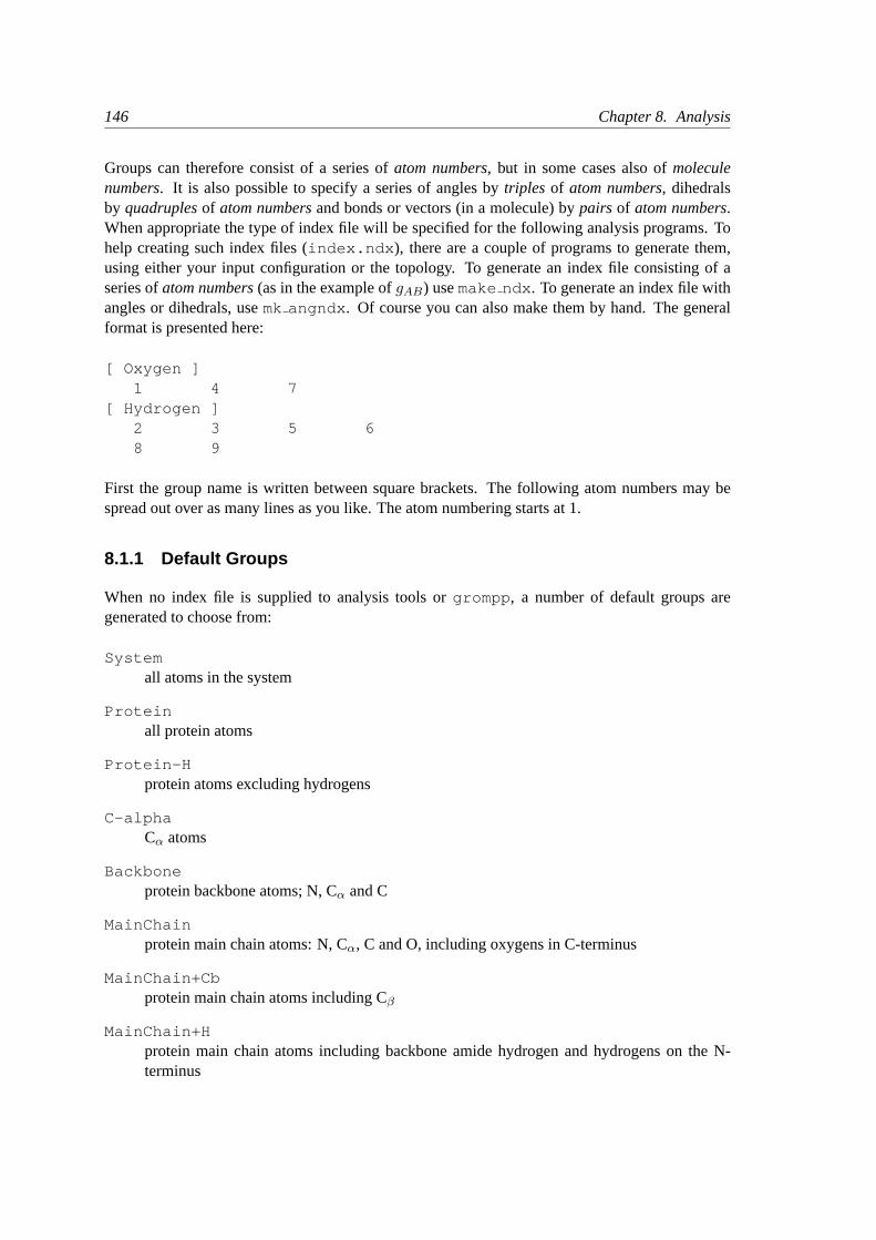
146 Chapter 8. Analysis
Groups can therefore consist of a series ofatom numbers, but in some cases also ofmoleculenumbers. It is also possible to specify a series of angles bytriples of atom numbers, dihedralsby quadruplesof atom numbersand bonds or vectors (in a molecule) bypairs of atom numbers.When appropriate the type of index file will be specified for the following analysis programs. Tohelp creating such index files (index.ndx ), there are a couple of programs to generate them,using either your input configuration or the topology. To generate an index file consisting of aseries ofatom numbers(as in the example ofgAB) usemake ndx . To generate an index file withangles or dihedrals, usemk angndx . Of course you can also make them by hand. The generalformat is presented here:
[ Oxygen ]1 4 7
[ Hydrogen ]2 3 5 68 9
First the group name is written between square brackets. The following atom numbers may bespread out over as many lines as you like. The atom numbering starts at 1.
8.1.1 Default Groups
When no index file is supplied to analysis tools orgrompp , a number of default groups aregenerated to choose from:
Systemall atoms in the system
Proteinall protein atoms
Protein-Hprotein atoms excluding hydrogens
C-alphaCα atoms
Backboneprotein backbone atoms; N, Cα and C
MainChainprotein main chain atoms: N, Cα, C and O, including oxygens in C-terminus
MainChain+Cbprotein main chain atoms including Cβ
MainChain+Hprotein main chain atoms including backbone amide hydrogen and hydrogens on the N-terminus
8.2. Looking at your trajectory 147
SideChainprotein side chain atoms; that is all atoms except N, Cα, C, O, backbone amide hydrogen,oxygens in C-terminus and hydrogens on the N-terminus
SideChain-Hprotein side chain atoms excluding all hydrogens
Prot-Massesprotein atoms excluding dummy masses (as used in dummy atom constructions of NH3
groups and Tryptophane sidechains), see also sec.5.2.2; this group is only included when itdiffers from the ’Protein ’ group
Non-Proteinall non-protein atoms
DNAall DNA atoms
molecule namefor all residues/molecules which are not recognized as protein or DNA, one group perresidue/molecule name is generated
Otherall atoms which are neither protein nor DNA.
Empty groups will not be generated. Most of the groups only contain protein atoms. An atom isconsidered a protein atom if its residue name is listed in theaminoacids.dat file.
8.2 Looking at your trajectory
ngmx
Before analyzing your trajectory it is often informative to look at your trajectory first. Gromacscomes with a simple trajectory viewerngmx; the advantage with this one is that it does not requireOpenGL, which usually isn’t present e.g. on supercomputers. It is also possible to generate a hard-copy in Encapsulated Postscript format, see Fig.8.1. If you want a faster and more fancy viewerthere are several programs that can read the GROMACS trajectory formats – have a look at ourhomepagewww.gromacs.orgfor updated links.
8.3 General properties
g_energyg_com
To analyze some or allenergiesand other properties, such astotal pressure, pressure tensor,density, box-volumeandbox-sizes, use the programg energy . A choice can be made from a list
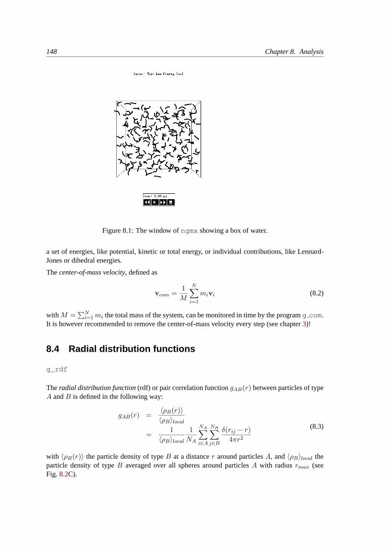
148 Chapter 8. Analysis
Figure 8.1: The window ofngmx showing a box of water.
a set of energies, like potential, kinetic or total energy, or individual contributions, like Lennard-Jones or dihedral energies.
Thecenter-of-mass velocity, defined as
vcom =1M
N∑i=1
mivi (8.2)
withM =∑N
i=1mi the total mass of the system, can be monitored in time by the programg com.It is however recommended to remove the center-of-mass velocity every step (see chapter3)!
8.4 Radial distribution functions
g_rdf
Theradial distribution function(rdf) or pair correlation functiongAB(r) between particles of typeA andB is defined in the following way:
gAB(r) =〈ρB(r)〉〈ρB〉local
=1
〈ρB〉local
1NA
NA∑i∈A
NB∑j∈B
δ(rij − r)4πr2
(8.3)
with 〈ρB(r)〉 the particle density of typeB at a distancer around particlesA, and〈ρB〉local theparticle density of typeB averaged over all spheres around particlesA with radiusrmax (seeFig. 8.2C).
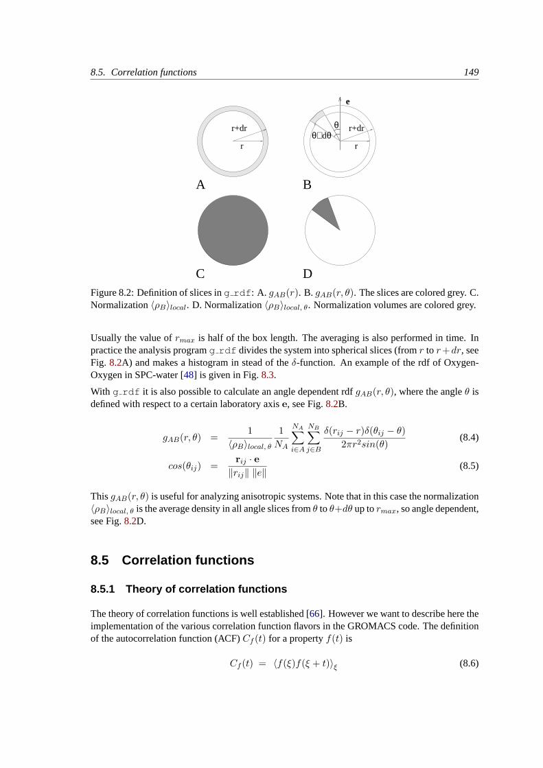
8.5. Correlation functions 149
r
r+dr r+dr
rθ+dθ
θ
e
A B
DCFigure 8.2: Definition of slices ing rdf : A. gAB(r). B. gAB(r, θ). The slices are colored grey. C.Normalization〈ρB〉local. D. Normalization〈ρB〉local, θ. Normalization volumes are colored grey.
Usually the value ofrmax is half of the box length. The averaging is also performed in time. Inpractice the analysis programg rdf divides the system into spherical slices (fromr to r+dr, seeFig. 8.2A) and makes a histogram in stead of theδ-function. An example of the rdf of Oxygen-Oxygen in SPC-water [48] is given in Fig.8.3.
With g rdf it is also possible to calculate an angle dependent rdfgAB(r, θ), where the angleθ isdefined with respect to a certain laboratory axise, see Fig.8.2B.
gAB(r, θ) =1
〈ρB〉local, θ
1NA
NA∑i∈A
NB∑j∈B
δ(rij − r)δ(θij − θ)2πr2sin(θ)
(8.4)
cos(θij) =rij · e
‖rij‖ ‖e‖(8.5)
ThisgAB(r, θ) is useful for analyzing anisotropic systems. Note that in this case the normalization〈ρB〉local, θ is the average density in all angle slices fromθ toθ+dθ up tormax, so angle dependent,see Fig.8.2D.
8.5 Correlation functions
8.5.1 Theory of correlation functions
The theory of correlation functions is well established [66]. However we want to describe here theimplementation of the various correlation function flavors in the GROMACS code. The definitionof the autocorrelation function (ACF)Cf (t) for a propertyf(t) is
Cf (t) = 〈f(ξ)f(ξ + t)〉ξ (8.6)
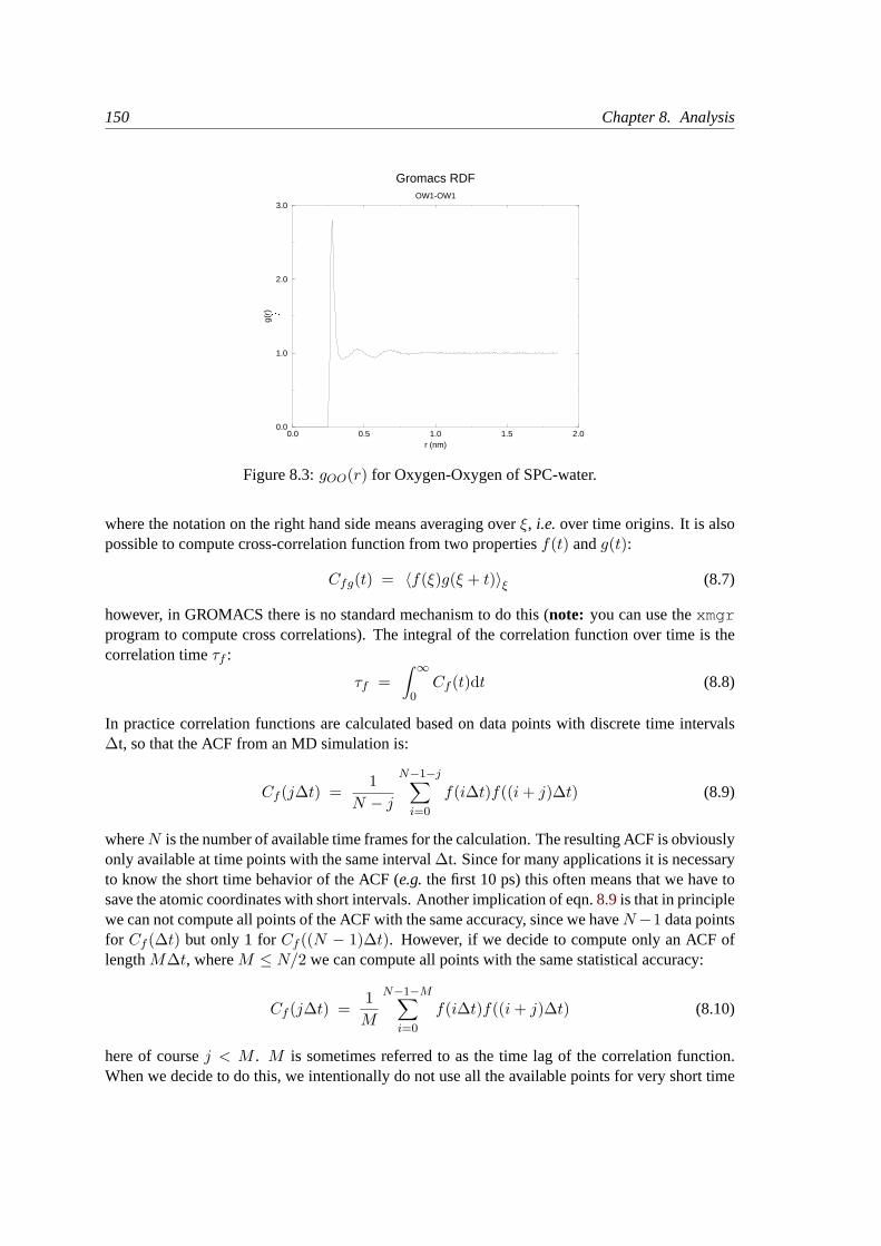
150 Chapter 8. Analysis
0.0 0.5 1.0 1.5 2.0r (nm)
0.0
1.0
2.0
3.0
g(r) �
Gromacs RDFOW1-OW1
Figure 8.3:gOO(r) for Oxygen-Oxygen of SPC-water.
where the notation on the right hand side means averaging overξ, i.e. over time origins. It is alsopossible to compute cross-correlation function from two propertiesf(t) andg(t):
Cfg(t) = 〈f(ξ)g(ξ + t)〉ξ (8.7)
however, in GROMACS there is no standard mechanism to do this (note: you can use thexmgrprogram to compute cross correlations). The integral of the correlation function over time is thecorrelation timeτf :
τf =∫ ∞
0Cf (t)dt (8.8)
In practice correlation functions are calculated based on data points with discrete time intervals∆t, so that the ACF from an MD simulation is:
Cf (j∆t) =1
N − j
N−1−j∑i=0
f(i∆t)f((i+ j)∆t) (8.9)
whereN is the number of available time frames for the calculation. The resulting ACF is obviouslyonly available at time points with the same interval∆t. Since for many applications it is necessaryto know the short time behavior of the ACF (e.g.the first 10 ps) this often means that we have tosave the atomic coordinates with short intervals. Another implication of eqn.8.9is that in principlewe can not compute all points of the ACF with the same accuracy, since we haveN−1 data pointsfor Cf (∆t) but only 1 forCf ((N − 1)∆t). However, if we decide to compute only an ACF oflengthM∆t, whereM ≤ N/2 we can compute all points with the same statistical accuracy:
Cf (j∆t) =1M
N−1−M∑i=0
f(i∆t)f((i+ j)∆t) (8.10)
here of coursej < M . M is sometimes referred to as the time lag of the correlation function.When we decide to do this, we intentionally do not use all the available points for very short time
8.5. Correlation functions 151
intervals (j << M ), but it makes it easier to interpret the results. Another aspect that may not beneglected when computing ACFs from simulation, is that usually the time originsξ (eqn.8.6) arenot statistically independent, which may introduce a bias in the results. This can be tested using ablock-averaging procedure, where only time origins with a spacing at least the length of the timelag are included,e.g.usingk time origins with spacing ofM∆t (wherekM ≤ N ):
Cf (j∆t) =1k
k−1∑i=0
f(iM∆t)f((iM + j)∆t) (8.11)
However, one needs very long simulations to get good accuracy this way, because there are manyfewer points that contribute to the ACF.
8.5.2 Using FFT for computation of the ACF
The computational cost for calculating an ACF according to eqn.8.9is proportional toN2, whichis considerable. However, this can be improved by using fast Fourier transforms to do the convo-lution [66].
8.5.3 Special forms of the ACF
There are some important varieties on the ACF,e.g.the ACF of a vectorp:
Cp(t) =∫ ∞
0Pn(cos 6 (p(t),p(t+ ξ)) dξ (8.12)
wherePn(x) is thenth order Legendre polynomial1. Such correlation times can actually be ob-tained experimentally usinge.g.NMR or other relaxation experiments. GROMACS can computecorrelations using the 1st and 2nd order Legendre polynomial (eqn.8.12). This can a.o. be usedfor rotational autocorrelation (g rotacf ), dipole autocorrelation (g dipoles ).
In order to study torsion angle dynamics we define a dihedral autocorrelation function as [67]:
C(t) = 〈cos(θ(τ)− θ(τ + t))〉τ (8.13)
Note that this is not a product of two functions as is generally used for correlation functions, but itmay be rewritten as the sum of two products:
C(t) = 〈cos(θ(τ)) cos(θ(τ + t)) + sin(θ(τ)) sin(θ(τ + t))〉τ (8.14)
8.5.4 Some Applications
The programg velacc calculates thisVelocity Auto Correlation Function.
Cv(τ) = 〈vi(τ) · vi(0)〉i∈A (8.15)
1P0(x) = 1, P1(x) = x, P2(x) = (3x2 − 1)/2
152 Chapter 8. Analysis
The self diffusion coefficient can be calculated using the Green-Kubo relation [66]
DA =13
∫ ∞
0〈vi(t) · vi(0)〉i∈A dt (8.16)
which is just the integral of the velocity autocorrelation function. There is a widely held beliefthat the velocity ACF converges faster than the mean square displacement (sec.8.5.5), which canalso be used for the computation of diffusion constants. However, Allen & Tildesly [66] warn usthat the long time contribution to the velocity ACF can not be ignored, so care must be taken.
Another important quantity is the dipole correlation time. Thedipole correlation functionforparticlesA is calculated as follows byg dipoles :
Cµ(τ) = 〈µi(τ) · µi(0)〉i∈A (8.17)
with µi =∑
j∈i rjqj . The dipole correlation time can be computed using eqn.8.8. For someapplications see [68].
The viscosity of a liquid can be related to the correlation time of the Pressure tensorP [69, 70].g energy can compute the viscosity, but this is not very accurate [65] (actually the values do notconverge...).
8.5.5 Mean Square Displacement
To determine the self diffusion coefficientDA of particlesA one can use the Einstein relation [66]
limt→∞
〈‖ri(t)− ri(0)‖2〉i∈A = 6DAt (8.18)
This Mean Square DisplacementandDA are calculated by the programg msd. For moleculesconsisting of more than one atom,ri is the center of mass positions. In that case you should usean index file with molecule numbers! The program can also be used for calculating diffusion inone or two dimensions. This is useful for studying lateral diffusion on interfaces.
An example of the mean square displacement of SPC-water is given in Fig.8.4.
8.6 Bonds, angles and dihedrals
g_bondg_angleg_sgangle
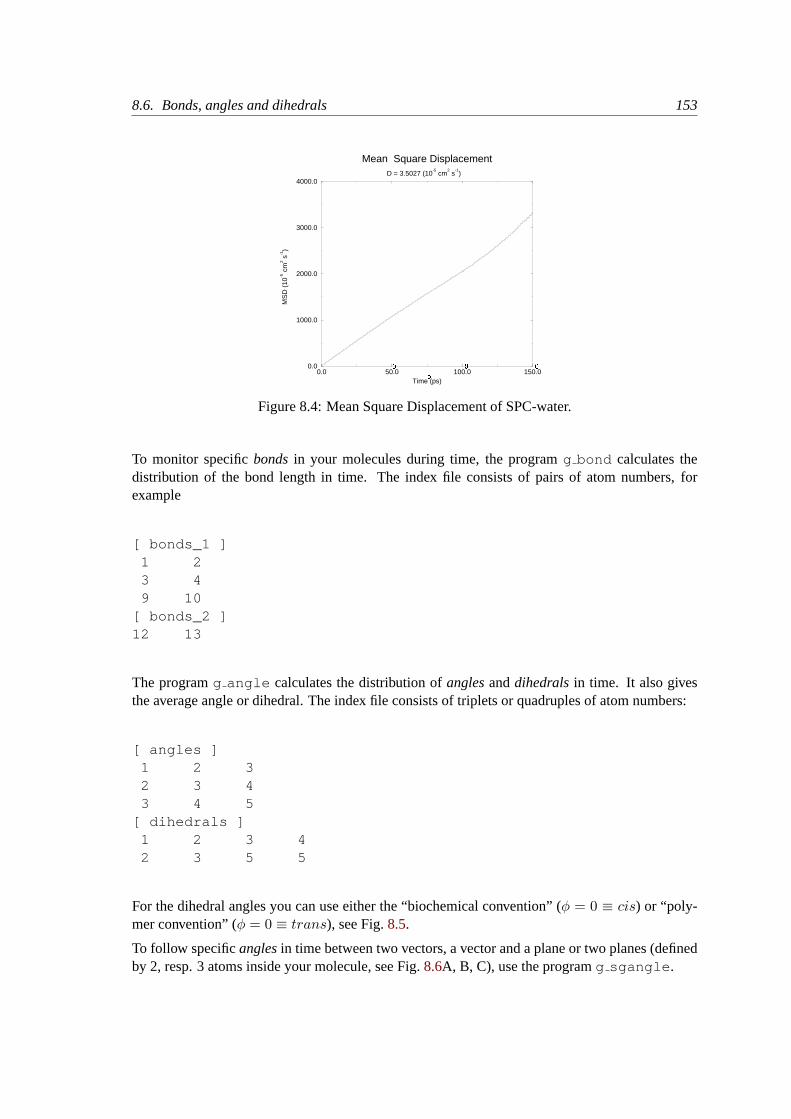
8.6. Bonds, angles and dihedrals 153
0.0 50.0�
100.0�
150.0�
Time (ps)�
0.0
1000.0
2000.0
3000.0
4000.0
MS
D (
10-5 c
m2 s
-1)
Mean Square DisplacementD = 3.5027 (10
-5 cm
2 s
-1)
Figure 8.4: Mean Square Displacement of SPC-water.
To monitor specificbondsin your molecules during time, the programg bond calculates thedistribution of the bond length in time. The index file consists of pairs of atom numbers, forexample
[ bonds_1 ]1 23 49 10
[ bonds_2 ]12 13
The programg angle calculates the distribution ofanglesanddihedralsin time. It also givesthe average angle or dihedral. The index file consists of triplets or quadruples of atom numbers:
[ angles ]1 2 32 3 43 4 5
[ dihedrals ]1 2 3 42 3 5 5
For the dihedral angles you can use either the “biochemical convention” (φ = 0 ≡ cis) or “poly-mer convention” (φ = 0 ≡ trans), see Fig.8.5.
To follow specificanglesin time between two vectors, a vector and a plane or two planes (definedby 2, resp. 3 atoms inside your molecule, see Fig.8.6A, B, C), use the programg sgangle .
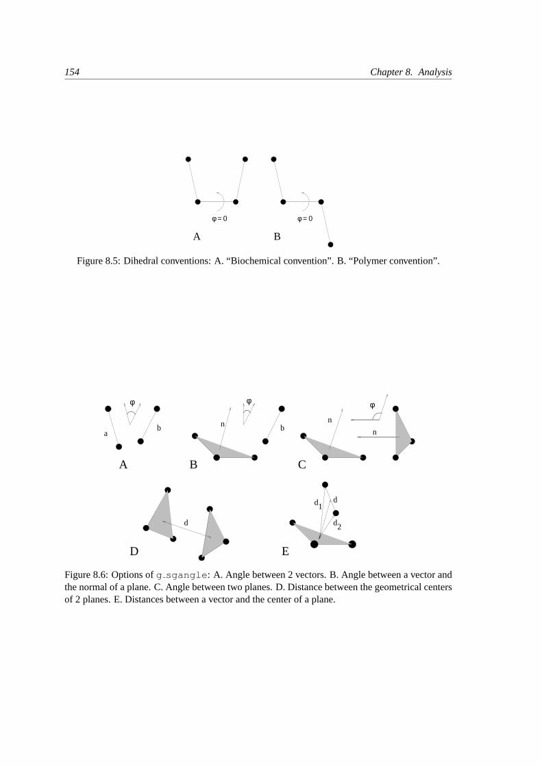
154 Chapter 8. Analysis
φ = 0φ = 0
A B
Figure 8.5: Dihedral conventions: A. “Biochemical convention”. B. “Polymer convention”.
b ba
φ
2
C
D
d
d
E
φ
d
φ
A B
n
1d
n
n
Figure 8.6: Options ofg sgangle : A. Angle between 2 vectors. B. Angle between a vector andthe normal of a plane. C. Angle between two planes. D. Distance between the geometrical centersof 2 planes. E. Distances between a vector and the center of a plane.
8.7. Radius of gyration and distances 155
For planes it uses the normal vector perpendicular to the plane. It can also calculate thedistancedbetween the geometrical center of two planes (see Fig.8.6D), and the distancesd1 andd2 between2 atoms (of a vector) and the center of a plane defined by 3 atoms (see Fig.8.6D). It furthercalculates the distanced between the center of the plane and the middle of this vector. Dependingon the input groups (i.e. groups of 2 or 3 atom numbers), the program decides what angles anddistances to calculate. For example, the index-file could look like this:
[ a_plane ]1 2 3
[ a_vector ]3 4 5
8.7 Radius of gyration and distances
g_gyrateg_sgangleg_mindistg_mdmatxpm2ps
To have a rough measure for the compactness of a structure, you can calculate theradius of gyra-tion with the programg gyrate as follows:
Rg =
(∑i ‖ri‖2mi∑
imi
) 12
(8.19)
wheremi is the mass of atomi andri the position of atomi with respect to the center of mass ofthe molecule. It is especially useful to characterize polymer solutions and proteins.
Sometimes it is interesting to plot thedistancebetween two atoms, or theminimumdistance be-tween two groups of atoms (e.g.: protein side-chains in a salt bridge). To calculate these distancesbetween certain groups there are several possibilities:
• Thedistance between the geometrical centersof two groups can be calculated with the programg sgangle , as explained in sec.8.6.
• The minimum distancebetween two groups of atoms during time can be calculated with theprogramg mindist . It also calculates thenumber of contactsbetween these groups withina certain radiusrmax.
• To monitor theminimum distances between residues(see chapter5) within a (protein) molecule,you can use the programg mdmat. This minimum distance between two residues Ai andAj is defined as the smallest distance between any pair of atoms (i∈ Ai, j ∈ Aj). The outputis a symmetrical matrix of smallest distances between all residues. To visualize this matrix,you can use a program such asxv . If you want to view the axes and legend or if you wantto print the matrix, you can convert it withxpm2ps into a Postscript picture, see Fig.8.7.
Plotting these matrices for different time-frames, one can analyze changes in the structure,ande.g.forming of salt bridges.

156 Chapter 8. Analysis
21 30 40 50 60 70 80 90
21
30
40
50
60
70
80
90
t=0
ps
Residue Number
0 Distance (nm) 1.2
Figure 8.7: A minimum distance matrix for a peptide [71].
8.8 Root mean square deviations in structure
g_rmsg_rmsdist
The root mean square deviation(RMSD) of certain atoms in a molecule with respect to a refer-ence structure can be calculated with the programg rms by least-square fitting the structure tothe reference structure (t2 = 0) and subsequently calculating theRMSD (eqn.8.20).
RMSD(t1, t2) =
[1M
N∑i=1
mi‖ri(t1)− ri(t2)‖2
] 12
(8.20)
whereM =∑N
i=1mi andri(t) is the position of atomi at timet. NOTE that fitting does nothave to use the same atoms as the calculation of theRMSD; e.g.: a protein is usually fitted onthe backbone atoms (N,Cα,C), but theRMSD can be computed of the backbone or of the wholeprotein.
Instead of comparing the structures to the initial structure at timet = 0 (so for example a crystalstructure), one can also calculate eqn.8.20with a structure at timet2 = t1 − τ . This gives someinsight in the mobility as a function ofτ . Also a matrix can be made with theRMSD as afunction oft1 andt2, this gives a nice graphical impression of a trajectory. If there are transitionsin a trajectory, they will clearly show up in such a matrix.
Alternatively theRMSD can be computed using a fit-free method with the programg rmsdist :
RMSD(t) =
1N2
N∑i=1
N∑j=1
‖rij(t)− rij(0)‖2
12
(8.21)
where thedistancer ij between atoms at timet is compared with the distance between the sameatoms at time0.
8.9. Covariance analysis 157
8.9 Covariance analysis
Covariance analysis, also called principal component analysis or essential dynamics [72], can findcorrelated motions. It uses the covariance matrixC of the atomic coordinates:
Cij =⟨M
12ii (xi − 〈xi〉)M
12jj(xj − 〈xj〉)
⟩(8.22)
whereM is a diagonal matrix containing the masses of the atoms (mass-weighted analysis) orthe unit matrix (non-mass weighted analysis).C is a symmetric3N × 3N matrix, which can bediagonalized with an orthonormal transformation matrixR:
RTCR = diag(λ1, λ2, . . . , λ3N ) where λ1 ≥ λ2 ≥ . . . ≥ λ3N (8.23)
The columns ofR are the eigenvectors, also called principal or essential modes.R defines atransformation to a new coordinate system. The trajectory can be projected on the principal modesto give the principal componentspi(t):
p(t) = RTM12 (x(t)− 〈x〉) (8.24)
The eigenvalueλi is the mean square fluctuation of principal componenti. The first few principalmodes often describe collective, global motions in the system. The trajectory can be filtered alongone (or more) principal modes. For one principal modei this goes as follows:
xf (t) = 〈x〉+M− 12R∗i pi(t) (8.25)
When the analysis is performed on a macromolecule, one often wants to remove the overall rota-tion and translation to look at the internal motion only. This can be achieved by least square fittingto a reference structure. Care has to be taken that the reference structure is representative for theensemble, since the choice of reference structure influences the covariance matrix.
One should always check if the principal modes are well defined. If the first principal componentresembles a half cosine and the second resembles a full cosine, you might be filtering noise (seebelow). A good way to check the relevance of the first few principal modes is to calculate theoverlap of the sampling between the first and second half of the simulation. Note that this canonly be done when the same reference structure is used for the two halves.
A good measure for the overlap has been defined in [73]. The elements of the covariance matrixare proportional to the square of the displacement, so we need to take the square root of the matrixto examine the extent of sampling. The square root can be calculated from the eigenvaluesλi andthe eigenvectors, which are the columns of the rotation matrixR. For a symmetric and diagonally-dominant matrixA of size3N × 3N the square root can be calculated as:
A12 = R diag(λ
121 , λ
122 , . . . , λ
123N )RT (8.26)
It can be verified easily that the product of this matrix with itself givesA. Now we can define adifferenced between covariance matricesA andB as follows:
d(A,B) =
√tr((A
12 −B
12
)2)
(8.27)
158 Chapter 8. Analysis
=√
tr(A+B − 2A
12B
12
)(8.28)
=
N∑i=1
(λA
i + λBi
)− 2
N∑i=1
N∑j=1
√λA
i λBj
(RA
i ·RBj
)2
12
(8.29)
where tr is the trace of a matrix. We can now define the overlaps as:
s(A,B) = 1− d(A,B)√trA+ trB
(8.30)
The overlap is 1 if and only if matricesA andB are identical. It is 0 when the sampled subspacesare completely orthogonal.
A commonly used measure is the subspace overlap of the first few eigenvectors of covariancematrices. The overlap of the subspace spanned bym orthonormal vectorsw1, . . . ,wm with areference subspace spanned byn orthonormal vectorsv1, . . . ,vn can be quantified as follows:
overlap(v,w) =1n
n∑i=1
m∑j=1
(vi ·wj)2 (8.31)
The overlap will increase with increasingm and will be 1 when setv is a subspace of setw. Thedisadvantage of this method is that it does not take the eigenvalues into account. All eigenvectorsare weighted equally and when degenerate subspaces are present (equal eigenvalues) the calculatedoverlap will be too low.
Another useful check is the cosine content. It has been proven the the principal components ofrandom diffusion are cosines with the number of periods equal to half the principal componentindex[74, 73]. The eigenvalues are proportional to the index to the power−2. The cosine contentis defined as:
2T
(∫ T
0cos(kπt) pi(t)dt
)2(∫ T
0p2
i (t)dt
)−1
(8.32)
When the cosine content of the first few principal components is close to 1, the largest fluctuationsare not connected with the potential, but with random diffusion.
The covariance matrix is built and diagonalized byg covar . The principal components andoverlap (any many more things) can be plotted and analyzed withg anaeig . The cosine contentcan be calculated withg analyze .
8.10 Hydrogen bonds
g_hbond
The programg hbond analyses thehydrogen bonds(H-bonds) between all possible donors D andacceptors A. To determine if an H-bond exists, a geometrical criterion is used, see also Fig.8.8:
r ≤ rHB = 0.35nmα ≤ αHB = 60o (8.33)
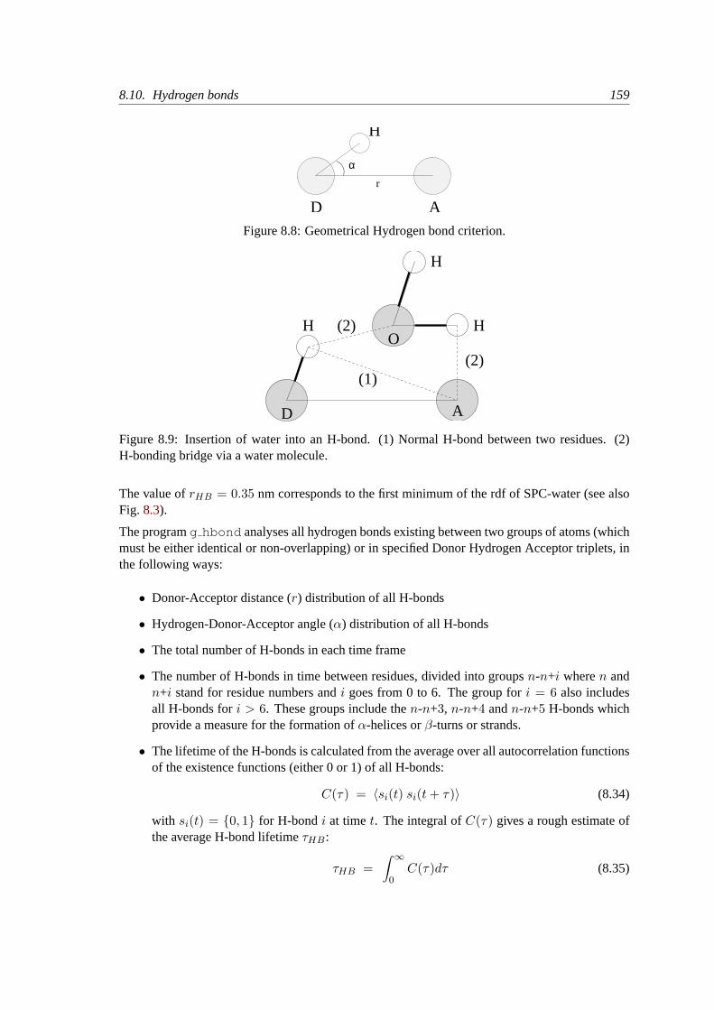
8.10. Hydrogen bonds 159
D
H
α
A
r
Figure 8.8: Geometrical Hydrogen bond criterion.
O
D A
H
H
H
(1)(2)
(2)
Figure 8.9: Insertion of water into an H-bond. (1) Normal H-bond between two residues. (2)H-bonding bridge via a water molecule.
The value ofrHB = 0.35 nm corresponds to the first minimum of the rdf of SPC-water (see alsoFig. 8.3).
The programg hbond analyses all hydrogen bonds existing between two groups of atoms (whichmust be either identical or non-overlapping) or in specified Donor Hydrogen Acceptor triplets, inthe following ways:
• Donor-Acceptor distance (r) distribution of all H-bonds
• Hydrogen-Donor-Acceptor angle (α) distribution of all H-bonds
• The total number of H-bonds in each time frame
• The number of H-bonds in time between residues, divided into groupsn-n+i wheren andn+i stand for residue numbers andi goes from 0 to 6. The group fori = 6 also includesall H-bonds fori > 6. These groups include then-n+3, n-n+4 andn-n+5 H-bonds whichprovide a measure for the formation ofα-helices orβ-turns or strands.
• The lifetime of the H-bonds is calculated from the average over all autocorrelation functionsof the existence functions (either 0 or 1) of all H-bonds:
C(τ) = 〈si(t) si(t+ τ)〉 (8.34)
with si(t) = {0, 1} for H-bondi at timet. The integral ofC(τ) gives a rough estimate ofthe average H-bond lifetimeτHB:
τHB =∫ ∞
0C(τ)dτ (8.35)
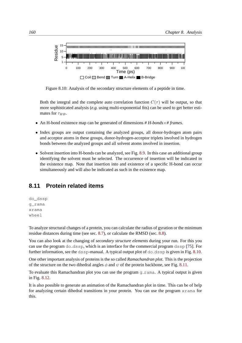
160 Chapter 8. Analysis
0 100 200 300 400 500 600 700 800 900 1000
1
5
10
15
Res
idue
Time (ps)Coil Bend Turn A-Helix B-Bridge
Figure 8.10: Analysis of the secondary structure elements of a peptide in time.
Both the integral and the complete auto correlation functionC(τ) will be output, so thatmore sophisticated analysis (e.g.using multi-exponential fits) can be used to get better esti-mates forτHB.
• An H-bond existence map can be generated of dimensions# H-bonds×# frames.
• Index groups are output containing the analyzed groups, all donor-hydrogen atom pairsand acceptor atoms in these groups, donor-hydrogen-acceptor triplets involved in hydrogenbonds between the analyzed groups and all solvent atoms involved in insertion.
• Solvent insertion into H-bonds can be analyzed, see Fig.8.9. In this case an additional groupidentifying the solvent must be selected. The occurrence of insertion will be indicated inthe existence map. Note that insertion into and existence of a specific H-bond can occursimultaneously and will also be indicated as such in the existence map.
8.11 Protein related items
do_dsspg_ramaxramawheel
To analyze structural changes of a protein, you can calculate the radius of gyration or the minimumresidue distances during time (see sec.8.7), or calculate the RMSD (sec.8.8).
You can also look at the changing ofsecondary structure elementsduring your run. For this youcan use the programdo dssp , which is an interface for the commercial programdssp [75]. Forfurther information, see thedssp -manual. A typical output plot ofdo dssp is given in Fig.8.10.
One other important analysis of proteins is the so calledRamachandran plot. This is the projectionof the structure on the two dihedral anglesφ andψ of the protein backbone, see Fig.8.11.
To evaluate this Ramachandran plot you can use the programg rama . A typical output is givenin Fig. 8.12.
It is also possible to generate an animation of the Ramachandran plot in time. This can be of helpfor analyzing certain dihedral transitions in your protein. You can use the programxrama forthis.
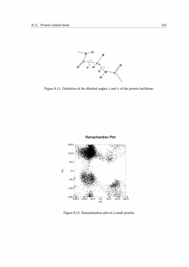
8.11. Protein related items 161
C
O
N
CH
R
C
Oα
N
H
H
ψφ
Figure 8.11: Definition of the dihedral anglesφ andψ of the protein backbone.
–180.0�
–120.0�
–60.0 0.0 60.0�
120.0�
180.0�
Phi
–180.0�
–120.0�
–60.0�
0.0
60.0
120.0
180.0
Psi
Ramachandran Plot
Figure 8.12: Ramachandran plot of a small protein.
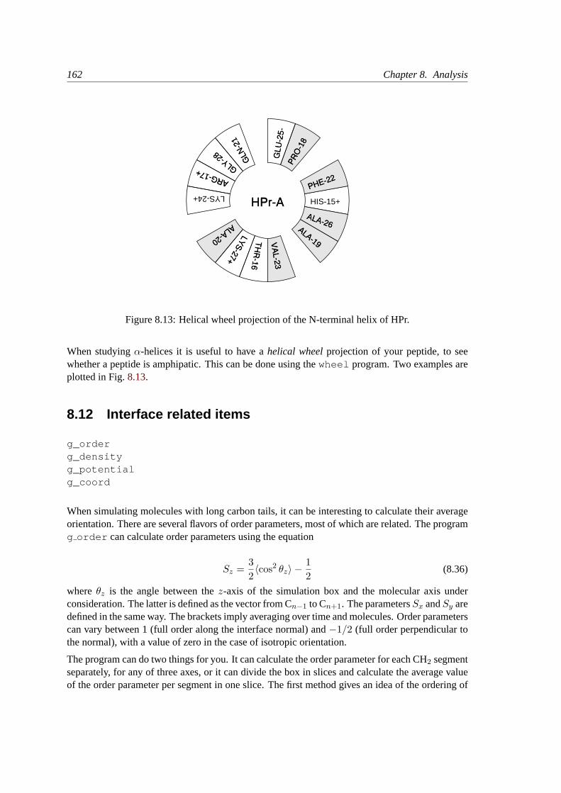
162 Chapter 8. Analysis
HPr-A HIS-15+
TH
R-16
ARG-17+
PRO
-18
ALA-19
ALA-20
GLN
-21
PHE-22
VA
L-23
LYS-24+
GLU
-25-
ALA-26
LYS-27+
GLY-28
Figure 8.13: Helical wheel projection of the N-terminal helix of HPr.
When studyingα-helices it is useful to have ahelical wheelprojection of your peptide, to seewhether a peptide is amphipatic. This can be done using thewheel program. Two examples areplotted in Fig.8.13.
8.12 Interface related items
g_orderg_densityg_potentialg_coord
When simulating molecules with long carbon tails, it can be interesting to calculate their averageorientation. There are several flavors of order parameters, most of which are related. The programg order can calculate order parameters using the equation
Sz =32〈cos2 θz〉 −
12
(8.36)
whereθz is the angle between thez-axis of the simulation box and the molecular axis underconsideration. The latter is defined as the vector from Cn−1 to Cn+1. The parametersSx andSy aredefined in the same way. The brackets imply averaging over time and molecules. Order parameterscan vary between 1 (full order along the interface normal) and−1/2 (full order perpendicular tothe normal), with a value of zero in the case of isotropic orientation.
The program can do two things for you. It can calculate the order parameter for each CH2 segmentseparately, for any of three axes, or it can divide the box in slices and calculate the average valueof the order parameter per segment in one slice. The first method gives an idea of the ordering of
8.13. Chemical shifts 163
a molecule from head to tail, the second method gives an idea of the ordering as function of thebox length.
The electrostatic potential (ψ) across the interface can be computed from a trajectory by evaluatingthe double integral of the charge density (ρ(z)):
ψ(z)− ψ(−∞) = −∫ z
−∞dz′
∫ z′
−∞ρ(z′′)dz′′/ε0 (8.37)
where the positionz = −∞ is far enough in the bulk phase that the field is zero. With thismethod, it is possible to “split” the total potential into separate contributions from lipid and watermolecules. The programg potential divides the box in slices and sums all charges of theatoms in each slice. It then integrates this charge density, giving the electric field, and the electricfield, giving the potential. Charge density, field and potential are written toxvgr- input files.
The programg coord is a very simple analysis program. All it does is print the coordinates ofselected atoms to three files, containing respectively thex-, y- andz-coordinates of those atoms.It can also calculate the center of mass of one or more molecules and print the coordinates of thecenter of mass to three files. By itself, this is probably not a very useful analysis, but having thecoordinates of selected molecules or atoms can be very handy for further analysis, not only ininterface systems.
The programg pvd calculates a lot of properties, among which the density of a group in particlesper unit of volume, but not a density that takes the mass of the atoms into account. The programg density also calculates the density of a group, but takes the masses into account and gives aplot of the density against a box axis. This is useful for looking at the distribution of groups oratoms across the interface.
8.13 Chemical shifts
totaldo_shift
You can compute the NMR chemical shifts of protons with the programdo shift . This is justan GROMACS interface to the public domain programtotal [76]. For further information, readthe article.

164 Chapter 8. Analysis

Appendix A
Technical Details
A.1 Installation
The entire GROMACS package is Free Software, licensed under the GNU General Public License.The main distribution site is our WWW server atwww.gromacs.org.
The package is mainly distributed as source code, but we also provide RPM packages for Linux.On the home page you will find all the information you need to install the package, mailing listswith archives, and several additional online resources like contributed topologies, etc. The defaultinstallation action is simply to unpack the source code and the issue
./configuremakemake install
The configuration script should automatically determine the best options for your platform, andit will tell you if anything is missing on your system. You will also find detailed step-by-stepinstallation instructions on the website.
A.2 Single or Double precision
GROMACS can be compiled in either single or double precision. The default choice is singleprecision, but it is easy to turn on double precision by selecting the--disable-float option tothe configuration script. Double precision will be 0 to 50% slower than single precision dependingon the architecture you are running on. Double precision will use somewhat more memory andrun input, energy and full-precision trajectory files will be almost twice as large. Note that theassembly loops are only available in single precision; Although the Intel SSE2 instruction set(available on Pentium IV and later) supports double precision instructions the performance ismuch lower than single precision. It would also mean very much extra work for a feature that veryfew people use, so we will probably not provide double precision assembly loops in the futureeither.
166 Appendix A. Technical Details
The energies in single precision are accurate up to the last decimal, the last one or two decimals ofthe forces are non-significant. The virial is less accurate than the forces, since the virial is only oneorder of magnitude larger than the size of each element in the sum over all atoms (sec.B.1). In mostcases this is not really a problem, since the fluctuations in de virial can be 2 orders of magnitudelarger than the average. In periodic charged systems these errors are often negligible. Especiallycut-off’s for the Coulomb interactions cause large errors in the energies, forces and virial. Evenwhen using a reaction-field or lattice sum method the errors are larger than or comparable tothe errors due to the single precision. Since MD is chaotic, trajectories with very similar startingconditions will diverge rapidly, the divergence is faster in single precision than in double precision.
For most simulations single precision is accurate enough. In some cases double precision is re-quired to get reasonable results:
• normal mode analysis, for the conjugate gradient minimization and the calculation and di-agonalization of the Hessian
• calculation of the constraint force between two large groups of atoms
• energy conservation (this can only be done without temperature coupling and without cut-off’s)
A.3 Porting GROMACS
The GROMACS system is designed with portability as a major design goal. However there area number of things we assume to be present on the system GROMACS is being ported on. Weassume the following features:
1. A UNIX-like operating system (BSD 4.x or SYSTEM V rev.3 or higher) or UNIX-likelibraries running under e.g. CygWin
2. an ANSI C compiler
3. optionally a Fortran-77 compiler or Fortran-90 compiler for faster (on some computers)inner loop routines
4. optionally the Nasm assembler to use the assembly innerloops on x86 processors.
There are some additional features in the package that require extra stuff to be present, but it ischecked for in the configuration script and you will be warned if anything important is missing.
That’s the requirements for a single processor system. If you want to compile GROMACS fora multiple processor environment you also need a MPI library (Message-Passing Interface) toperform the parallel communication. This is always shipped with supercomputers, and for work-stations you can find links to free MPI implementations through the GROMACS homepage atwww.gromacs.org.
A.4. Environment Variables 167
A.3.1 Multi-processor Optimization
If you want to, you could write your own optimized communication (perhaps using specific li-braries for your hardware) instead of MPI. This should never be necessary for normal use (wehaven’t heard of a modern computer where it isn’t possible to run MPI), but if you absolutely wantto do it, here are some clues.
The interface between the communication routines and the rest of the GROMACS system is de-scribed in the file$GMXHOME/src/include/network.h We will give a short description ofthe different routines below.
extern void gmx tx(int pid,void *buf,int bufsize);This routine, when called with the destination processor number, a pointer to a (byte ori-ented) transfer buffer, and the size of the buffer will send the buffer to the indicated processor(in our case always the neighboring processor). The routine doesnot wait until the transferis finished.
extern void gmx tx wait(int pid);This routine waits until the previous, or the ongoing transmission is finished.
extern void gmx txs(int pid,void *buf,int bufsize);This routine implements a synchronous send by calling the a-synchronous routine and thenthe wait. It might come in handy to code this differently.
extern void gmx rx(int pid,void *buf,int bufsize);
extern void gmx rx wait(int pid);
extern void gmx rxs(int pid,void *buf,int bufsize);The very same routines for receiving a buffer and waiting until the reception is finished.
extern void gmx init(int pid,int nprocs);This routine initializes the different devices needed to do the communication. In general itsets up the communication hardware (if it is accessible) or does an initialize call to the lowerlevel communication subsystem.
extern void gmx stat(FILE *fp,char *msg);With this routine we can diagnose the ongoing communication. In the current implemen-tation it prints the various contents of the hardware communication registers of the (Inteli860) multiprocessor boards to a file.
A.4 Environment Variables
GROMACS programs may be influenced by the use of environment variables. First of all, the vari-ables set in the GMXRC file are essential for running and compiling GROMACS. Other variablesare:
1. DUMPNL, dump neighbor list. If set to a positive number theentireneighbor list is printedin the log file (may be many megabytes). Mainly for debugging purposes, but may also behandy for porting to other platforms.
168 Appendix A. Technical Details
2. IAMCOOL, if this is explicitly set to NO your GROMACS life will be dull and boring. (i.e.,no cool quotes).
3. WHERE, when set print debugging info on line numbers.
4. LOGBUFS, the size of the buffer for file I/O. When set to 0, all file I/O will be unbufferedand therefore very slow. This can be handy for debugging purposes, because it ensures thatall files are always totally up-to-date.
5. GMXNPRI, for SGI systems only. When set, gives the default non-degrading priority (npri)for mdrun , nmrun , g covar andg nmeig , e.g.settingsetenv GMXNPRI 250 causesall runs to be performed at near-lowest priority by default.
6. GMXVIEW XPM, GMXVIEW XVG, GMXVIEW EPSandGMXVIEW PDB, commands usedto automatically view resp..xvg , .xpm , .eps and .pdb file types; they default toxv ,xmgrace , ghostview and rasmol . Set to empty to disable automatic viewing of aparticular file type. The command will be forked off and run in the background at the samepriority as the GROMACS tool (which might not be what you want). Be careful not to usea command which blocks the terminal (e.g.vi ), since multiple instances might be run.
Some other environment variables are specific to one program, such as TOTAL for thedo shiftprogram, and DSPP for thedo dssp program.
A.5 Running GROMACS in parallel
If you have installed the MPI (Message Passing Interface) on your computer(s) you can compileGROMACS with this library to run simulations in parallel. All supercomputers are shipped withMPI libraries optimized for that particular platform, and if you are using a cluster of workstationsthere are several good free MPI implementations. You can find updated links to these on the gro-macs homepagewww.gromacs.org. Once you have an MPI library installed it’s trivial to compileGROMACS with MPI support: Just set the option--enable-mpi to the configure script andrecompile. (But don’t forget to make distclean before running configure if you have previouslycompiled with a different configuration.) If you are using a supercomputer you might also want toturn of the default nicing of the mdrun process with the--disable-nice option.
There is usually a program calledmpirun with which you can fire up the parallel processes. Atypical command line looks like:% mpirun -p goofus,doofus,fred 10 mdrun -s topol -v -N 30this runs on each of the machines goofus,doofus,fred with 10 processes on each1.
If you have a single machine with multiple processors you don’t have to use thempirun com-mand, but you can do with an extra option tomdrun :% mdrun -np 8 -s topol -v -N 8In this example MPI reads the first option from the command line. Sincemdrun also wants toknow the number of processes you have to type it twice.
Check your local manuals (or online manual) for exact details of your MPI implementation.
1Example taken from Silicon Graphics manual

A.5. Running GROMACS in parallel 169
If you are interested in programming MPI yourself, you can find manuals and reference literatureon the internet.

170 Appendix A. Technical Details
Appendix B
Some implementation details
In this chapter we will present some implementation details. This is far from complete, but wedeemed it necessary to clarify some things that would otherwise be hard to understand.
B.1 Single Sum Virial in GROMACS.
The virialΞ can be written in full tensor form as:
Ξ = − 12
N∑i<j
rij ⊗ F ij (B.1)
where⊗ denotes thedirect productof two vectors1. When this is computed in the inner loop ofan MD program 9 multiplications and 9 additions are needed2.
Here it is shown how it is possible to extract the virial calculation from the inner loop [77].
B.1.1 Virial.
In a system with Periodic Boundary Conditions, the periodicity must be taken into account for thevirial:
Ξ = − 12
N∑i<j
rnij ⊗ F ij (B.2)
wherernij denotes the distance vector of thenearest imageof atomi from atomj. In this definition
we add ashift vectorδi to the position vectorri of atomi. The difference vectorrnij is thus equal
to:rn
ij = ri + δi − rj (B.3)
or in shorthand:rn
ij = rni − rj (B.4)
1(u⊗ v)αβ = uαvβ2The calculation of Lennard-Jones and Coulomb forces is about 50 floating point operations.
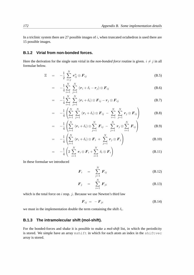
172 Appendix B. Some implementation details
In a triclinic system there are 27 possible images ofi, when truncated octahedron is used there are15 possible images.
B.1.2 Virial from non-bonded forces.
Here the derivation for the single sum virial in thenon-bonded forceroutine is given.i 6= j in allformulae below.
Ξ = −12
N∑i<j
rnij ⊗ F ij (B.5)
= −14
N∑i=1
N∑j=1
(ri + δi − rj)⊗ F ij (B.6)
= −14
N∑i=1
N∑j=1
(ri + δi)⊗ F ij − rj ⊗ F ij (B.7)
= −14
N∑i=1
N∑j=1
(ri + δi)⊗ F ij −N∑
i=1
N∑j=1
rj ⊗ F ij
(B.8)
= −14
N∑i=1
(ri + δi)⊗N∑
j=1
F ij −N∑
j=1
rj ⊗N∑
i=1
F ij
(B.9)
= −14
N∑i=1
(ri + δi)⊗ F i +N∑
j=1
rj ⊗ F j
(B.10)
= −14
(2
N∑i=1
ri ⊗ F i +N∑
i=1
δi ⊗ F i
)(B.11)
In these formulae we introduced
F i =N∑
j=1
F ij (B.12)
F j =N∑
i=1
F ji (B.13)
which is the total force oni resp.j. Because we use Newton’s third law
F ij = − F ji (B.14)
we must in the implementation double the term containing the shiftδi.
B.1.3 The intramolecular shift (mol-shift).
For the bonded-forces and shake it is possible to make amol-shift list, in which the periodicityis stored. We simple have an arraymshift in which for each atom an index in theshiftvecarray is stored.
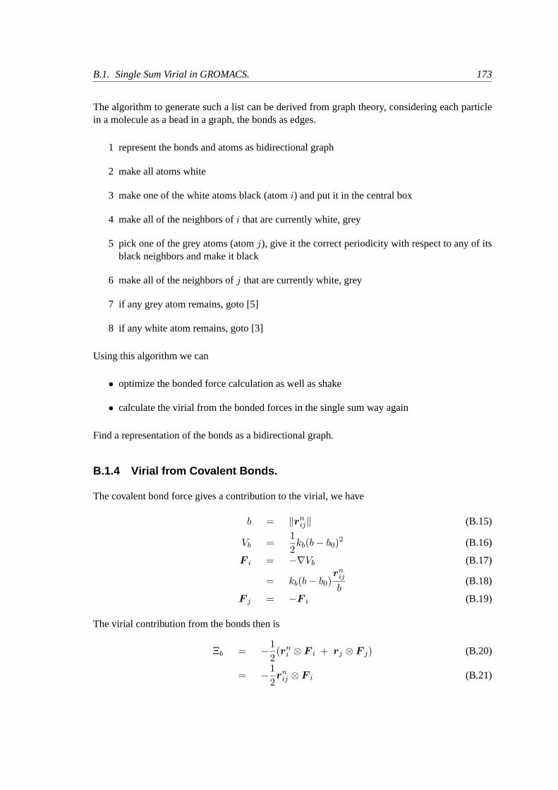
B.1. Single Sum Virial in GROMACS. 173
The algorithm to generate such a list can be derived from graph theory, considering each particlein a molecule as a bead in a graph, the bonds as edges.
1 represent the bonds and atoms as bidirectional graph
2 make all atoms white
3 make one of the white atoms black (atomi) and put it in the central box
4 make all of the neighbors ofi that are currently white, grey
5 pick one of the grey atoms (atomj), give it the correct periodicity with respect to any of itsblack neighbors and make it black
6 make all of the neighbors ofj that are currently white, grey
7 if any grey atom remains, goto [5]
8 if any white atom remains, goto [3]
Using this algorithm we can
• optimize the bonded force calculation as well as shake
• calculate the virial from the bonded forces in the single sum way again
Find a representation of the bonds as a bidirectional graph.
B.1.4 Virial from Covalent Bonds.
The covalent bond force gives a contribution to the virial, we have
b = ‖rnij‖ (B.15)
Vb =12kb(b− b0)2 (B.16)
F i = −∇Vb (B.17)
= kb(b− b0)rn
ij
b(B.18)
F j = −F i (B.19)
The virial contribution from the bonds then is
Ξb = −12(rn
i ⊗ F i + rj ⊗ F j) (B.20)
= −12rn
ij ⊗ F i (B.21)
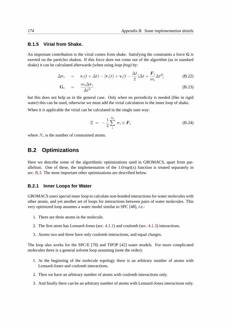
174 Appendix B. Some implementation details
B.1.5 Virial from Shake.
An important contribution to the virial comes from shake. Satisfying the constraints a forceG isexerted on the particles shaken. If this force does not come out of the algorithm (as in standardshake) it can be calculated afterwards (when usingleap-frog) by:
∆ri = ri(t+ ∆t)− [ri(t) + vi(t−∆t2
)∆t+F i
mi∆t2] (B.22)
Gi =mi∆ri
∆t2(B.23)
but this does not help us in the general case. Only when no periodicity is needed (like in rigidwater) this can be used, otherwise we must add the virial calculation in the inner loop of shake.
When it is applicable the virial can be calculated in the single sum way:
Ξ = − 12
Nc∑i
ri ⊗ F i (B.24)
whereNc is the number of constrained atoms.
B.2 Optimizations
Here we describe some of the algorithmic optimizations used in GROMACS, apart from par-allelism. One of these, the implementation of the 1.0/sqrt(x) function is treated separately insec.B.3. The most important other optimizations are described below.
B.2.1 Inner Loops for Water
GROMACS users special inner loop to calculate non-bonded interactions for water molecules withother atoms, and yet another set of loops for interactions between pairs of water molecules. Thisvery optimized loop assumes a water model similar to SPC [48], i.e.:
1. There are three atoms in the molecule.
2. The first atom has Lennard-Jones (sec.4.1.1) and coulomb (sec.4.1.3) interactions.
3. Atoms two and three have only coulomb interactions, and equal charges.
The loop also works for the SPC/E [78] and TIP3P [42] water models. For more complicatedmolecules there is a general solvent loop assuming (note the order):
1. At the beginning of the molecule topology there is an arbitrary number of atoms withLennard-Jones and coulomb interactions.
2. Then we have an arbitrary number of atoms with coulomb interactions only.
3. And finally there can be an arbitrary number of atoms with Lennard-Jones interactions only.
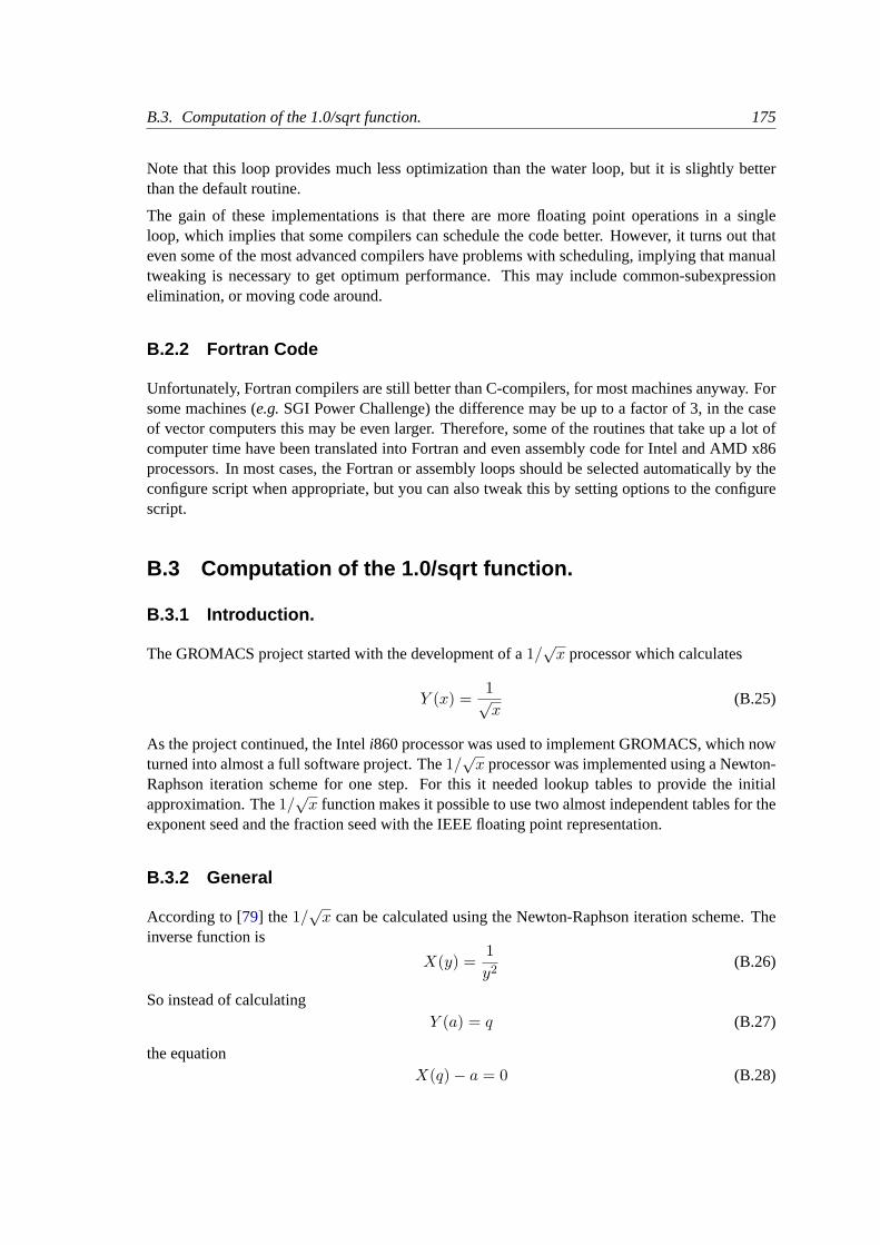
B.3. Computation of the 1.0/sqrt function. 175
Note that this loop provides much less optimization than the water loop, but it is slightly betterthan the default routine.
The gain of these implementations is that there are more floating point operations in a singleloop, which implies that some compilers can schedule the code better. However, it turns out thateven some of the most advanced compilers have problems with scheduling, implying that manualtweaking is necessary to get optimum performance. This may include common-subexpressionelimination, or moving code around.
B.2.2 Fortran Code
Unfortunately, Fortran compilers are still better than C-compilers, for most machines anyway. Forsome machines (e.g.SGI Power Challenge) the difference may be up to a factor of 3, in the caseof vector computers this may be even larger. Therefore, some of the routines that take up a lot ofcomputer time have been translated into Fortran and even assembly code for Intel and AMD x86processors. In most cases, the Fortran or assembly loops should be selected automatically by theconfigure script when appropriate, but you can also tweak this by setting options to the configurescript.
B.3 Computation of the 1.0/sqrt function.
B.3.1 Introduction.
The GROMACS project started with the development of a1/√x processor which calculates
Y (x) =1√x
(B.25)
As the project continued, the Inteli860 processor was used to implement GROMACS, which nowturned into almost a full software project. The1/
√x processor was implemented using a Newton-
Raphson iteration scheme for one step. For this it needed lookup tables to provide the initialapproximation. The1/
√x function makes it possible to use two almost independent tables for the
exponent seed and the fraction seed with the IEEE floating point representation.
B.3.2 General
According to [79] the 1/√x can be calculated using the Newton-Raphson iteration scheme. The
inverse function is
X(y) =1y2
(B.26)
So instead of calculatingY (a) = q (B.27)
the equationX(q)− a = 0 (B.28)
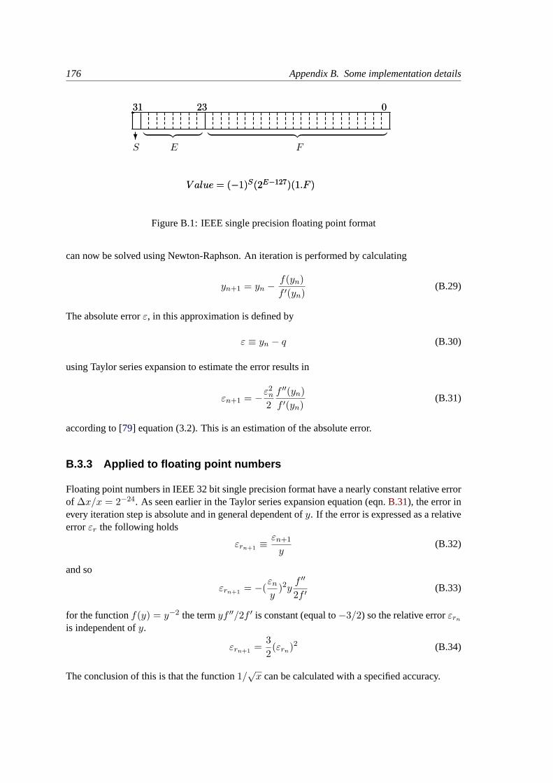
176 Appendix B. Some implementation details
︸ ︷︷ ︸︸ ︷︷ ︸?FES
02331
V alue = (−1)S(2E−127)(1.F )
02331
V alue = (−1)S(2E−127)(1.F )
Figure B.1: IEEE single precision floating point format
can now be solved using Newton-Raphson. An iteration is performed by calculating
yn+1 = yn −f(yn)f ′(yn)
(B.29)
The absolute errorε, in this approximation is defined by
ε ≡ yn − q (B.30)
using Taylor series expansion to estimate the error results in
εn+1 = −ε2n
2f ′′(yn)f ′(yn)
(B.31)
according to [79] equation (3.2). This is an estimation of the absolute error.
B.3.3 Applied to floating point numbers
Floating point numbers in IEEE 32 bit single precision format have a nearly constant relative errorof ∆x/x = 2−24. As seen earlier in the Taylor series expansion equation (eqn.B.31), the error inevery iteration step is absolute and in general dependent ofy. If the error is expressed as a relativeerrorεr the following holds
εrn+1 ≡εn+1
y(B.32)
and so
εrn+1 = −(εny
)2yf ′′
2f ′(B.33)
for the functionf(y) = y−2 the termyf ′′/2f ′ is constant (equal to−3/2) so the relative errorεrn
is independent ofy.
εrn+1 =32(εrn)2 (B.34)
The conclusion of this is that the function1/√x can be calculated with a specified accuracy.
B.3. Computation of the 1.0/sqrt function. 177
B.3.4 Specification of the lookup table
To calculate the function1/√x using the previously mentioned iteration scheme, it is clear that the
first estimation of the solution must be accurate enough to get precise results. The requirementsfor the calculation are
• Maximum possible accuracy with the used IEEE format
• Use only one iteration step for maximum speed
The first requirement states that the result of1/√x may have a relative errorεr equal to the
εr of a IEEE 32 bit single precision floating point number. From this the1/√x of the initial
approximation can be derived, rewriting the definition of the relative error for succeeding steps,equation (eqn.B.34)
εny
=
√εrn+1
2f ′
yf ′′(B.35)
So for the lookup table the needed accuracy is
∆YY
=√
232−24 (B.36)
which defines the width of the table that must be≥ 13 bit.
At this point the relative errorεrn of the lookup table is known. From this the maximum relativeerror in the argument can be calculated as follows. The absolute error∆x is defined as
∆x ≡ ∆YY ′
(B.37)
and thus∆xY
=∆YY
(Y ′)−1 (B.38)
and thus
∆x = constantY
Y ′(B.39)
for the 1/√x functionY/Y ′ ∼ x holds, so∆x/x = constant. This is a property of the used
floating point representation as earlier mentioned. The needed accuracy of the argument of thelookup table follows from
∆xx
= −2∆YY
(B.40)
so, using the floating point accuracy, equation (eqn.B.36)
∆xx
= −2√
232−24 (B.41)
This defines the length of the lookup table which should be≥ 12 bit.

178 Appendix B. Some implementation details
B.3.5 Separate exponent and fraction computation
The used IEEE 32 bit single precision floating point format specifies that a number is representedby a exponent and a fraction. The previous section specifies for every possible floating pointnumber the lookup table length and width. Only the size of the fraction of a floating point numberdefines the accuracy. The conclusion from this can be that the size of the lookup table is length oflookup table, earlier specified, times the size of the exponent (21228, 1Mb). The1/
√x function
has the property that the exponent is independent of the fraction. This becomes clear if the floatingpoint representation is used. Define
x ≡ (−1)S(2E−127)(1.F ) (B.42)
see Fig.B.1 where0 ≤ S ≤ 1, 0 ≤ E ≤ 255, 1 ≤ 1.F < 2 andS, E, F integer (normalizationconditions). The sign bit (S) can be omitted because1/
√x is only defined forx > 0. The1/
√x
function applied tox results in
y(x) =1√x
(B.43)
or
y(x) =1√
(2E−127)(1.F )(B.44)
this can be rewritten asy(x) = (2E−127)−1/2(1.F )−1/2 (B.45)
Define(2E′−127) ≡ (2E−127)−1/2 (B.46)
1.F ′ ≡ (1.F )−1/2 (B.47)
then 1√2< 1.F ′ ≤ 1 holds, so the condition1 ≤ 1.F ′ < 2 which is essential for normalized real
representation is not valid anymore. By introducing an extra term this can be corrected. Rewritethe1/
√x function applied to floating point numbers, equation (eqn.B.45) as
y(x) = (2127−E
2−1)(2(1.F )−1/2) (B.48)
and(2E′−127) ≡ (2
127−E2
−1) (B.49)
1.F ′ ≡ 2(1.F )−1/2 (B.50)
then√
2 < 1.F ≤ 2 holds. This is not the exact valid range as defined for normalized floatingpoint numbers in equation (eqn.B.42). The value2 causes the problem. By mapping this valueon the nearest representation< 2 this can be solved. The small error that is introduced by thisapproximation is within the allowable range.
The integer representation of the exponent is the next problem. Calculating(2127−E
2−1) introduces
a fractional result if(127 − E) = odd. This is again easily accounted for by splitting up thecalculation into an odd and an even part. For(127 − E) = even E′ in equation (eqn.B.49) canbe exactly calculated in integer arithmetic as a function ofE.
E′ =127− E
2+ 126 (B.51)
B.3. Computation of the 1.0/sqrt function. 179
For (127− E) = odd equation (eqn.B.45) can be rewritten as
y(x) = (2127−E−1
2 )(1.F2
)−1/2 (B.52)
thus
E′ =126− E
2+ 127 (B.53)
which also can be calculated exactly in integer arithmetic. Note that the fraction is automaticallycorrected for its range earlier mentioned, so the exponent does not need an extra correction.
The conclusions from this are:
• The fraction and exponent lookup table are independent. The fraction lookup table existsof two tables (odd and even exponent) so the odd/even information of the exponent (lsb bit)has to be used to select the right table.
• The exponent table is an 256 x 8 bit table, initialized forodd andeven.
B.3.6 Implementation
The lookup tables can be generated by a small C program, which uses floating point numbersand operations with IEEE 32 bit single precision format. Note that because of theodd/eveninformation that is needed, the fraction table is twice the size earlier specified (13 bit i.s.o. 12 bit).
The function according to equation (eqn.B.29) has to be implemented. Applied to the1/√x
function, equation (eqn.B.28) leads to
f = a− 1y2
(B.54)
and so
f ′ =2y3
(B.55)
so
yn+1 = yn −a− 1
y2n
2y3
n
(B.56)
oryn+1 =
yn
2(3− ay2
n) (B.57)
Wherey0 can be found in the lookup tables, andy1 gives the result to the maximum accuracy. Itis clear that only one iteration extra (in double precision) is needed for a double precision result.

180 Appendix B. Some implementation details
Appendix C
Long range corrections
C.1 Dispersion
In this section we derive long range corrections due to the use of a cut-off for Lennard Jonesinteractions. We assume that the cut-off is so long that the repulsion term can safely be neglected,and therefore only the dispersion term is taken into account. Due to the nature of the dispersioninteraction, energy and pressure corrections both are negative. While the energy correction isusually small, it may be important for free energy calculations. The pressure correction in contrastis very large and can not be neglected. Although it is in principle possible to parameterize a forcefield such that the pressure is close to 1 bar even without correction, such a method makes theparameterization dependent on the cut-off and is therefore undesirable. Please note that it is notconsistent to use the long range correction to the dispersion without using either a reaction fieldmethod or a proper long range electrostatics method such as Ewald summation or PPPM.
C.1.1 Energy
The long range contribution of the dispersion interaction to the virial can be derived analytically, ifwe assume a homogeneous system beyond the cut-off distancerc. The dispersion energy betweentwo particles is written as:
V (rij) = − C6r−6ij (C.1)
and the corresponding force isF ij = − 6C6r
−8ij rij (C.2)
The long range contribution to the dispersion energy in a system withN particles and particledensityρ =N/V , whereV is the volume, is [66]:
Vlr =12Nρ
∫ ∞
rc
4πr2g(r)V (r)dr (C.3)
which we can integrate assuming that the radial distribution functiong(r) is 1 beyond the cut-offrc
Vlr = − 23NρπC6r
−3c (C.4)

182 Appendix C. Long range corrections
If we consider for example a box of pure water, simulated with a cut-off of 0.9 nm and a densityof 1 g cm−3 this correction is -0.25 kJ mol−1.
For a homogeneous mixture ofM componentsj with Nj particles each, we can write the longrange contribution to the energy as:
Vlr =M∑i6=j
−2NiNj
3VπC6(ij)r−3
c (C.5)
This can be rewritten if we define anaverage dispersion constant〈C6〉:
〈C6〉 =∑i6=j
NiNj
N2C6(ij) (C.6)
Vlr = −23Nρπ 〈C6〉 r−3
c (C.7)
A special form of a non-homogeneous system in this respect, is a pure liquid in which the atomshave differentC6 values. In practice this definition encompasses almost every molecule, exceptmono-atomic molecules and symmetric molecules likeN2 or O2. Therefore we always have todetermine the average dispersion constant〈C6〉 in simulations.
In the case of inhomogeneous simulation systems,e.g.a system with a lipid interface, the energycorrection can be applied if〈C6〉 for both components is comparable.
C.1.2 Virial and pressure
The scalar virial of the system due to the dispersion interaction between two particlesi andj isgiven by:
Ξ = − rij · F ij = 6C6r−6ij (C.8)
The pressure is given by:
P =2
3V(Ekin − Ξ) (C.9)
We can again integrate the long range contribution to the virial [66]:
Ξlr =12Nρ
∫ ∞
rc
4πr2 Ξdr
= 12NπρC6
∫ ∞
rc
r−4ij dr
= 4πC6Nρr−3c (C.10)
The corresponding correction to the pressure is
Plr = − 43πC6ρ
2r−3c (C.11)
Using the same example of a water box, the correction to the virial is 3 kJ mol−1 the correspondingcorrection to the pressure for SPC water at liquid density is approx. -280 bar.
C.1. Dispersion 183
For homogeneous mixtures we can again use the average dispersion constant〈C6〉 (eqn.C.6):
Plr = − 43π 〈C6〉 ρ2r−3
c (C.12)
For inhomogeneous systems eqn.C.12can be applied under the same restriction as holds for theenergy (see sec.C.1.1).

184 Appendix C. Long range corrections
Appendix D
Averages and fluctuations
D.1 Formulae for averaging
Note: this section was taken from ref [80].
When analyzing a MD trajectory averages〈x〉 and fluctuations
⟨(∆x)2
⟩ 12 =
⟨[x− 〈x〉]2
⟩ 12 (D.1)
of a quantityx are to be computed. The varianceσx of a series of Nx values,{xi}, can be computedfrom
σx =Nx∑i=1
x2i − 1
Nx
(Nx∑i=1
xi
)2
(D.2)
Unfortunately this formula is numerically not very accurate, especially whenσ12x is small compared
to the values ofxi. The following (equivalent) expression is numerically more accurate
σx =Nx∑i=1
[xi − 〈x〉]2 (D.3)
with
〈x〉 =1Nx
Nx∑i=1
xi (D.4)
Using eqns.D.2 andD.4 one has to go through the series ofxi values twice, once to determine〈x〉 and again to computeσx, whereas eqn.D.1 requires only one sequential scan of the series{xi}. However, one may cast eqn.D.2 in another form, containing partial sums, which allows fora sequential update algorithm. Define the partial sum
Xn,m =m∑
i=n
xi (D.5)
186 Appendix D. Averages and fluctuations
and the partial variance
σn,m =m∑
i=n
[xi −
Xn,m
m− n+ 1
]2(D.6)
It can be shown thatXn,m+k = Xn,m +Xm+1,m+k (D.7)
and
σn,m+k = σn,m + σm+1,m+k +[
Xn,m
m− n+ 1− Xn,m+k
m+ k − n+ 1
]2∗
(m− n+ 1)(m+ k − n+ 1)k
(D.8)
Forn = 1 one finds
σ1,m+k = σ1,m + σm+1,m+k +[X1,m
m− X1,m+k
m+ k
]2 m(m+ k)k
(D.9)
and forn = 1 andk = 1 (eqn.D.8) becomes
σ1,m+1 = σ1,m +[X1,m
m− X1,m+1
m+ 1
]2m(m+ 1) (D.10)
= σ1,m +[ X1,m −mxm+1 ]2
m(m+ 1)(D.11)
where we have used the relation
X1,m+1 = X1,m + xm+1 (D.12)
Using formulae (eqn.D.11) and (eqn.D.12) the average
〈x〉 =X1,Nx
Nx(D.13)
and the fluctuation ⟨(∆x)2
⟩ 12 =
[σ1,Nx
Nx
] 12
(D.14)
can be obtained by one sweep through the data.
D.2 Implementation
In GROMACS the instantaneous energiesE(m) are stored in the energy file, along with the valuesof σ1,m andX1,m. Although the steps are counted from 0, for the energy and fluctuations steps arecounted from 1. This means that the equations presented here are the ones that are implemented.We give somewhat lengthy derivations in this section to simplify checking of code and equationslater on.
D.2. Implementation 187
D.2.1 Part of a Simulation
It is not uncommon to perform a simulation where the first part,e.g.100 ps, is taken as equili-bration. However, the averages and fluctuations as printed in the log file are computed over thewhole simulation. The equilibration time, which is now part of the simulation, may in such a caseinvalidate the averages and fluctuations, because these numbers are now dominated by the initialdrift towards equilibrium.
Using eqns.D.7 andD.8 the average and standard deviation over part of the trajectory can becomputed as:
Xm+1,m+k = X1,m+k −X1,m (D.15)
σm+1,m+k = σ1,m+k − σ1,m −[X1,m
m− X1,m+k
m+ k
]2 m(m+ k)k
(D.16)
or, more generally (withp ≥ 1 andq ≥ p):
Xp,q = X1,q −X1,p−1 (D.17)
σp,q = σ1,q − σ1,p−1 −[X1,p−1
p− 1− X1,q
q
]2 (p− 1)qq − p+ 1
(D.18)
Note that implementation of this is not entirely trivial, since energies are not stored every timestep of the simulation. We therefore have to constructX1,p−1 andσ1,p−1 from the information attimep using eqns.D.11andD.12:
X1,p−1 = X1,p − xp (D.19)
σ1,p−1 = σ1,p −[ X1,p−1 − (p− 1)xp ]2
(p− 1)p(D.20)
D.2.2 Combining two simulations
Another frequently occurring problem is, that the fluctuations of two simulations must be com-bined. Consider the following example: we have two simulations (A) ofn and (B) ofm steps, inwhich the second simulation is a continuation of the first. However, the second simulation startsnumbering from 1 instead of fromn + 1. For the partial sum this is no problem, we have to addXA
1,n from run A:
XAB1,n+m = XA
1,n +XB1,m (D.21)
When we want to compute the partial variance from the two components we have to make acorrection∆σ:
σAB1,n+m = σA
1,n + σB1,m + ∆σ (D.22)
if we definexABi as the combined and renumbered set of data points we can write:
σAB1,n+m =
n+m∑i=1
[xAB
i −XAB
1,n+m
n+m
]2
(D.23)

188 Appendix D. Averages and fluctuations
and thus
n+m∑i=1
[xAB
i −XAB
1,n+m
n+m
]2
=n∑
i=1
[xA
i −XA
1,n
n
]2
+m∑
i=1
[xB
i −XB
1,m
m
]2
+ ∆σ (D.24)
or
n+m∑i=1
(xABi )2 − 2xAB
i
XAB1,n+m
n+m+
(XAB
1,n+m
n+m
)2 −
n∑i=1
(xAi )2 − 2xA
i
XA1,n
n+
(XA
1,n
n
)2 −
m∑i=1
(xBi )2 − 2xB
i
XB1,m
m+
(XB
1,m
m
)2 = ∆σ (D.25)
all thex2i terms drop out, and the terms independent of the summation counteri can be simplified:(
XAB1,n+m
)2
n+m−
(XA
1,n
)2
n−
(XB
1,m
)2
m−
2XAB
1,n+m
n+m
n+m∑i=1
xABi + 2
XA1,n
n
n∑i=1
xAi + 2
XB1,m
m
m∑i=1
xBi = ∆σ (D.26)
we recognize the three partial sums on the second line and use eqn.D.21to obtain:
∆σ =
(mXA
1,n − nXB1,m
)2
nm(n+m)(D.27)
if we check this by insertingm = 1 we get back eqn.D.11
D.2.3 Summing energy terms
The genergy program can also sum energy terms into one,e.g.potential + kinetic = total. For thepartial averages this is again easy if we haveS energy componentss:
XSm,n =
n∑i=m
S∑s=1
xsi =
S∑s=1
n∑i=m
xsi =
S∑s=1
Xsm,n (D.28)
For the fluctuations it is less trivial again, considering for example that the fluctuation in potentialand kinetic energy should cancel. Nevertheless we can try the same approach as before by writing:
σSm,n =
S∑s=1
σsm,n + ∆σ (D.29)
if we fill in eqn. D.6:
n∑i=m
[(S∑
s=1
xsi
)−
XSm,n
m− n+ 1
]2
=S∑
s=1
n∑i=m
[(xs
i )−Xs
m,n
m− n+ 1
]2+ ∆σ (D.30)
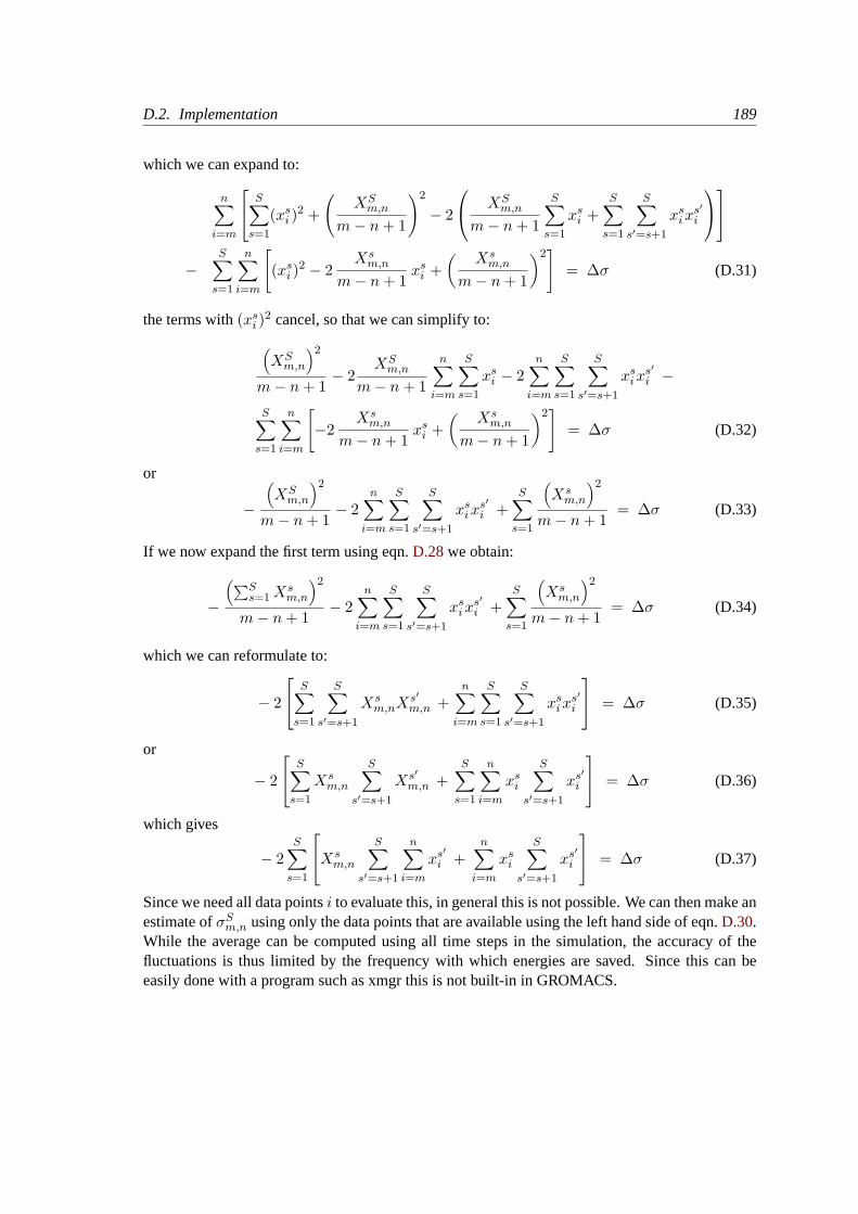
D.2. Implementation 189
which we can expand to:
n∑i=m
S∑s=1
(xsi )
2 +
(XS
m,n
m− n+ 1
)2
− 2
XSm,n
m− n+ 1
S∑s=1
xsi +
S∑s=1
S∑s′=s+1
xsix
s′i
−
S∑s=1
n∑i=m
[(xs
i )2 − 2
Xsm,n
m− n+ 1xs
i +(
Xsm,n
m− n+ 1
)2]
= ∆σ (D.31)
the terms with(xsi )
2 cancel, so that we can simplify to:(XS
m,n
)2
m− n+ 1− 2
XSm,n
m− n+ 1
n∑i=m
S∑s=1
xsi − 2
n∑i=m
S∑s=1
S∑s′=s+1
xsix
s′i −
S∑s=1
n∑i=m
[−2
Xsm,n
m− n+ 1xs
i +(
Xsm,n
m− n+ 1
)2]
= ∆σ (D.32)
or
−
(XS
m,n
)2
m− n+ 1− 2
n∑i=m
S∑s=1
S∑s′=s+1
xsix
s′i +
S∑s=1
(Xs
m,n
)2
m− n+ 1= ∆σ (D.33)
If we now expand the first term using eqn.D.28we obtain:
−
(∑Ss=1X
sm,n
)2
m− n+ 1− 2
n∑i=m
S∑s=1
S∑s′=s+1
xsix
s′i +
S∑s=1
(Xs
m,n
)2
m− n+ 1= ∆σ (D.34)
which we can reformulate to:
− 2
S∑s=1
S∑s′=s+1
Xsm,nX
s′m,n +
n∑i=m
S∑s=1
S∑s′=s+1
xsix
s′i
= ∆σ (D.35)
or
− 2
S∑s=1
Xsm,n
S∑s′=s+1
Xs′m,n +
S∑s=1
n∑i=m
xsi
S∑s′=s+1
xs′i
= ∆σ (D.36)
which gives
− 2S∑
s=1
Xsm,n
S∑s′=s+1
n∑i=m
xs′i +
n∑i=m
xsi
S∑s′=s+1
xs′i
= ∆σ (D.37)
Since we need all data pointsi to evaluate this, in general this is not possible. We can then make anestimate ofσS
m,n using only the data points that are available using the left hand side of eqn.D.30.While the average can be computed using all time steps in the simulation, the accuracy of thefluctuations is thus limited by the frequency with which energies are saved. Since this can beeasily done with a program such as xmgr this is not built-in in GROMACS.

190 Appendix D. Averages and fluctuations
Appendix E
Manual Pages
E.1 options
All GROMACS programs have 6 standard options, of which some are hidden by default:
Other options-h bool no Print help info and quit-X bool no Use dialog box GUI to edit command line options
-nice int 0 Set the nicelevel
• If the configuration script found Motif or Lesstif on your system, you can use the graphical interface(if not, you will get an error):-X boolno Use dialog box GUI to edit command line options
• When compiled on an SGI-IRIX system, all GROMACS programs have an additional option:-npri int 0 Set non blocking priority (try 128)
• Optional files are not used unless the option is set, in contrast to non optional files, where the defaultfile name is used when the option is not set.
• All GROMACS programs will accept file options without a file extension or filename being specified.In such cases the default filenames will be used. With multiple input file types, such as genericstructure format, the directory will be searched for files of each type with the supplied or defaultname. When no such file is found, or with output files the first file type will be used.
• All GROMACS programs with the exception ofmdrun , nmrun andeneconv check if the com-mand line options are valid. If this is not the case, the program will be halted.
• Enumerated options (enum) should be used with one of the arguments listed in the option description,the argument may be abbreviated. The first match to the shortest argument in the list will be selected.
• Vector options can be used with 1 or 3 parameters. When only one parameter is supplied the twoothers are also set to this value.
• For many GROMACS programs, the time options can be supplied in different time units, dependingon the setting of the-tu option.
• All GROMACS programs can read compressed or g-zipped files. There might be a problem withreading compressed.xtc , .trr and.trj files, but these will not compress very well anyway.
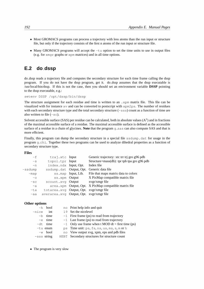
192 Appendix E. Manual Pages
• Most GROMACS programs can process a trajectory with less atoms than the run input or structurefile, but only if the trajectory consists of the first n atoms of the run input or structure file.
• Many GROMACS programs will accept the-tu option to set the time units to use in output files(e.g. forxmgr graphs orxpm matrices) and in all time options.
E.2 do dssp
do dssp reads a trajectory file and computes the secondary structure for each time frame calling the dsspprogram. If you do not have the dssp program, get it. dodssp assumes that the dssp executable is/usr/local/bin/dssp. If this is not the case, then you should set an environment variableDSSPpointingto the dssp executable, e.g.:
setenv DSSP /opt/dssp/bin/dssp
The structure assignment for each residue and time is written to an.xpm matrix file. This file can bevisualized with for instancexv and can be converted to postscript withxpm2ps . The number of residueswith each secondary structure type and the total secondary structure (-sss ) count as a function of time arealso written to file (-sc ).
Solvent accessible surface (SAS) per residue can be calculated, both in absolute values (A2) and in fractionsof the maximal accessible surface of a residue. The maximal accessible surface is defined as the accessiblesurface of a residue in a chain of glycines.Note that the programg sas can also compute SAS and that ismore efficient.
Finally, this program can dump the secondary structure in a special filessdump.dat for usage in theprogramg chi . Together these two programs can be used to analyze dihedral properties as a function ofsecondary structure type.
Files-f traj.xtc Input Generic trajectory: xtc trr trj gro g96 pdb-s topol.tpr Input Structure+mass(db): tpr tpb tpa gro g96 pdb-n index.ndx Input, Opt. Index file
-ssdump ssdump.dat Output, Opt. Generic data file-map ss.map Input, Lib. File that maps matrix data to colors
-o ss.xpm Output X PixMap compatible matrix file-sc scount.xvg Output xvgr/xmgr file
-a area.xpm Output, Opt. X PixMap compatible matrix file-ta totarea.xvg Output, Opt. xvgr/xmgr file-aa averarea.xvg Output, Opt. xvgr/xmgr file
Other options-h bool no Print help info and quit
-nice int 19 Set the nicelevel-b time -1 First frame (ps) to read from trajectory-e time -1 Last frame (ps) to read from trajectory
-dt time -1 Only use frame when t MOD dt = first time (ps)-tu enum ps Time unit: ps , fs , ns , us , ms, s , mor h
-w bool no View output xvg, xpm, eps and pdb files-sss string HEBT Secondary structures for structure count
• The program is very slow
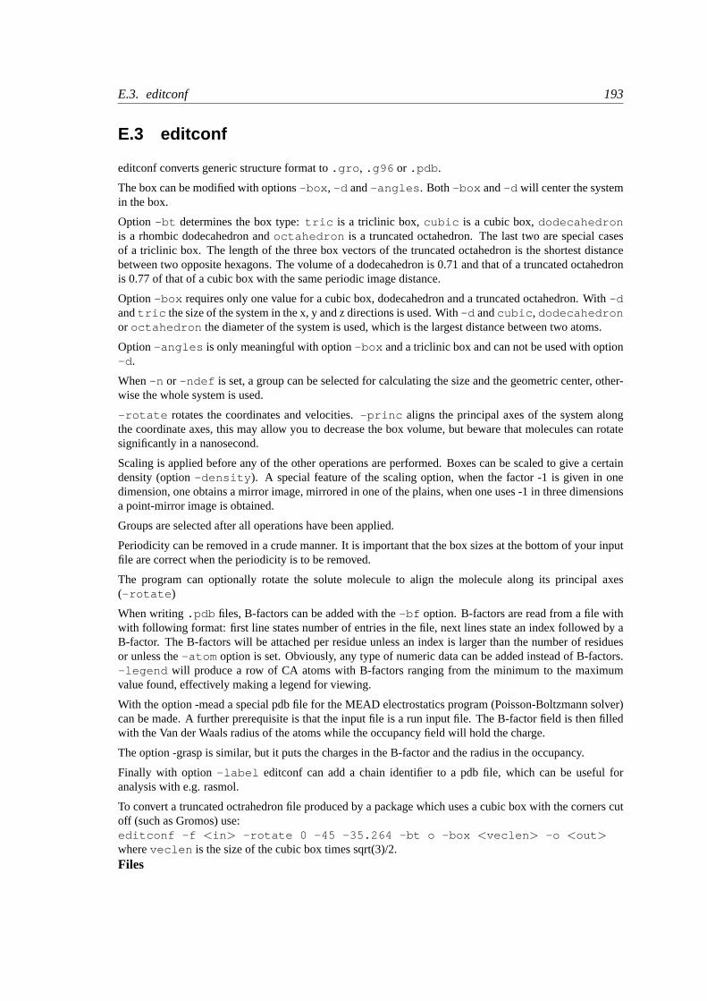
E.3. editconf 193
E.3 editconf
editconf converts generic structure format to.gro , .g96 or .pdb .
The box can be modified with options-box , -d and-angles . Both-box and-d will center the systemin the box.
Option -bt determines the box type:tric is a triclinic box,cubic is a cubic box,dodecahedronis a rhombic dodecahedron andoctahedron is a truncated octahedron. The last two are special casesof a triclinic box. The length of the three box vectors of the truncated octahedron is the shortest distancebetween two opposite hexagons. The volume of a dodecahedron is 0.71 and that of a truncated octahedronis 0.77 of that of a cubic box with the same periodic image distance.
Option-box requires only one value for a cubic box, dodecahedron and a truncated octahedron. With-dandtric the size of the system in the x, y and z directions is used. With-d andcubic , dodecahedronor octahedron the diameter of the system is used, which is the largest distance between two atoms.
Option-angles is only meaningful with option-box and a triclinic box and can not be used with option-d .
When-n or -ndef is set, a group can be selected for calculating the size and the geometric center, other-wise the whole system is used.
-rotate rotates the coordinates and velocities.-princ aligns the principal axes of the system alongthe coordinate axes, this may allow you to decrease the box volume, but beware that molecules can rotatesignificantly in a nanosecond.
Scaling is applied before any of the other operations are performed. Boxes can be scaled to give a certaindensity (option-density ). A special feature of the scaling option, when the factor -1 is given in onedimension, one obtains a mirror image, mirrored in one of the plains, when one uses -1 in three dimensionsa point-mirror image is obtained.
Groups are selected after all operations have been applied.
Periodicity can be removed in a crude manner. It is important that the box sizes at the bottom of your inputfile are correct when the periodicity is to be removed.
The program can optionally rotate the solute molecule to align the molecule along its principal axes(-rotate )
When writing.pdb files, B-factors can be added with the-bf option. B-factors are read from a file withwith following format: first line states number of entries in the file, next lines state an index followed by aB-factor. The B-factors will be attached per residue unless an index is larger than the number of residuesor unless the-atom option is set. Obviously, any type of numeric data can be added instead of B-factors.-legend will produce a row of CA atoms with B-factors ranging from the minimum to the maximumvalue found, effectively making a legend for viewing.
With the option -mead a special pdb file for the MEAD electrostatics program (Poisson-Boltzmann solver)can be made. A further prerequisite is that the input file is a run input file. The B-factor field is then filledwith the Van der Waals radius of the atoms while the occupancy field will hold the charge.
The option -grasp is similar, but it puts the charges in the B-factor and the radius in the occupancy.
Finally with option -label editconf can add a chain identifier to a pdb file, which can be useful foranalysis with e.g. rasmol.
To convert a truncated octrahedron file produced by a package which uses a cubic box with the corners cutoff (such as Gromos) use:editconf -f <in > -rotate 0 -45 -35.264 -bt o -box <veclen > -o <out >whereveclen is the size of the cubic box times sqrt(3)/2.Files
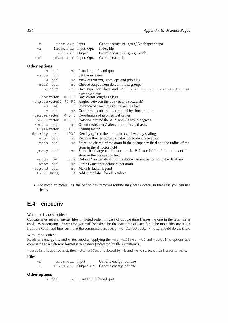
194 Appendix E. Manual Pages
-f conf.gro Input Generic structure: gro g96 pdb tpr tpb tpa-n index.ndx Input, Opt. Index file-o out.gro Output Generic structure: gro g96 pdb
-bf bfact.dat Input, Opt. Generic data file
Other options-h bool no Print help info and quit
-nice int 0 Set the nicelevel-w bool no View output xvg, xpm, eps and pdb files
-ndef bool no Choose output from default index groups-bt enum tric Box type for -box and -d: tric , cubic , dodecahedron or
octahedron-box vector 0 0 0 Box vector lengths (a,b,c)
-angles vector90 90 90 Angles between the box vectors (bc,ac,ab)-d real 0 Distance between the solute and the box-c bool no Center molecule in box (implied by -box and -d)
-center vector 0 0 0 Coordinates of geometrical center-rotate vector 0 0 0 Rotation around the X, Y and Z axes in degrees
-princ bool no Orient molecule(s) along their principal axes-scale vector 1 1 1 Scaling factor
-density real 1000 Density (g/l) of the output box achieved by scaling-pbc bool no Remove the periodicity (make molecule whole again)
-mead bool no Store the charge of the atom in the occupancy field and the radius of theatom in the B-factor field
-grasp bool no Store the charge of the atom in the B-factor field and the radius of theatom in the occupancy field
-rvdw real 0.12 Default Van der Waals radius if one can not be found in the database-atom bool no Force B-factor attachment per atom
-legend bool no Make B-factor legend-label string A Add chain label for all residues
• For complex molecules, the periodicity removal routine may break down, in that case you can usetrjconv
E.4 eneconv
When-f is notspecified:Concatenates several energy files in sorted order. In case of double time frames the one in the later file isused. By specifying-settime you will be asked for the start time of each file. The input files are takenfrom the command line, such that the commandeneconv -o fixed.edr *.edr should do the trick.
With -f specified:Reads one energy file and writes another, applying the-dt , -offset , -t0 and-settime options andconverting to a different format if necessary (indicated by file extentions).
-settime is applied first, then-dt /-offset followed by-b and-e to select which frames to write.
Files-f ener.edr Input Generic energy: edr ene-o fixed.edr Output, Opt. Generic energy: edr ene
Other options-h bool no Print help info and quit
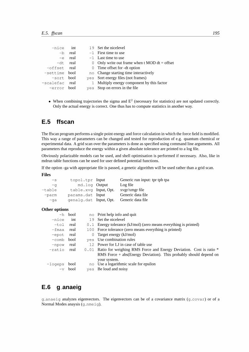
E.5. ffscan 195
-nice int 19 Set the nicelevel-b real -1 First time to use-e real -1 Last time to use
-dt real 0 Only write out frame when t MOD dt = offset-offset real 0 Time offset for -dt option
-settime bool no Change starting time interactively-sort bool yes Sort energy files (not frames)
-scalefac real 1 Multiply energy component by this factor-error bool yes Stop on errors in the file
• When combining trajectories the sigma and E2 (necessary for statistics) are not updated correctly.Only the actual energy is correct. One thus has to compute statistics in another way.
E.5 ffscan
The ffscan program performs a single point energy and force calculation in which the force field is modified.This way a range of parameters can be changed and tested for reproduction of e.g. quantum chemical orexperimental data. A grid scan over the parameters is done as specified using command line arguments. Allparameters that reproduce the energy within a given absolute tolerance are printed to a log file.
Obviously polarizable models can be used, and shell optimisation is performed if necessary. Also, like inmdrun table functions can be used for user defined potential functions.
If the option -ga with appropriate file is passed, a genetic algorithm will be used rather than a grid scan.
Files-s topol.tpr Input Generic run input: tpr tpb tpa-g md.log Output Log file
-table table.xvg Input, Opt. xvgr/xmgr file-parm params.dat Input Generic data file
-ga genalg.dat Input, Opt. Generic data file
Other options-h bool no Print help info and quit
-nice int 19 Set the nicelevel-tol real 0.1 Energy tolerance (kJ/mol) (zero means everything is printed)
-fmax real 100 Force tolerance (zero means everything is printed)-epot real 0 Target energy (kJ/mol)-comb bool yes Use combination rules-npow real 12 Power for LJ in case of table use
-ratio real 0.01 Ratio for weighing RMS Force and Energy Deviation. Cost is ratio *RMS Force + abs(Energy Deviation). This probably should depend onyour system.
-logeps bool no Use a logarithmic scale for epsilon-v bool yes Be loud and noisy
E.6 g anaeig
g anaeig analyzes eigenvectors. The eigenvectors can be of a covariance matrix (g covar ) or of aNormal Modes anaysis (g nmeig ).
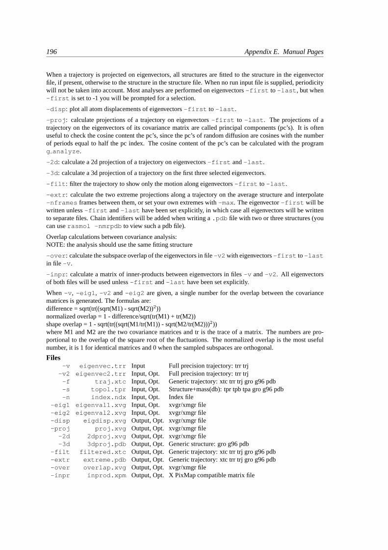
196 Appendix E. Manual Pages
When a trajectory is projected on eigenvectors, all structures are fitted to the structure in the eigenvectorfile, if present, otherwise to the structure in the structure file. When no run input file is supplied, periodicitywill not be taken into account. Most analyses are performed on eigenvectors-first to -last , but when-first is set to -1 you will be prompted for a selection.
-disp : plot all atom displacements of eigenvectors-first to -last .
-proj : calculate projections of a trajectory on eigenvectors-first to -last . The projections of atrajectory on the eigenvectors of its covariance matrix are called principal components (pc’s). It is oftenuseful to check the cosine content the pc’s, since the pc’s of random diffusion are cosines with the numberof periods equal to half the pc index. The cosine content of the pc’s can be calculated with the programg analyze .
-2d : calculate a 2d projection of a trajectory on eigenvectors-first and-last .
-3d : calculate a 3d projection of a trajectory on the first three selected eigenvectors.
-filt : filter the trajectory to show only the motion along eigenvectors-first to -last .
-extr : calculate the two extreme projections along a trajectory on the average structure and interpolate-nframes frames between them, or set your own extremes with-max . The eigenvector-first will bewritten unless-first and-last have been set explicitly, in which case all eigenvectors will be writtento separate files. Chain identifiers will be added when writing a.pdb file with two or three structures (youcan userasmol -nmrpdb to view such a pdb file).
Overlap calculations between covariance analysis:NOTE: the analysis should use the same fitting structure
-over : calculate the subspace overlap of the eigenvectors in file-v2 with eigenvectors-first to -lastin file -v .
-inpr : calculate a matrix of inner-products between eigenvectors in files-v and-v2 . All eigenvectorsof both files will be used unless-first and-last have been set explicitly.
When -v , -eig1 , -v2 and -eig2 are given, a single number for the overlap between the covariancematrices is generated. The formulas are:difference = sqrt(tr((sqrt(M1) - sqrt(M2))2))normalized overlap = 1 - difference/sqrt(tr(M1) + tr(M2))shape overlap = 1 - sqrt(tr((sqrt(M1/tr(M1)) - sqrt(M2/tr(M2)))2))where M1 and M2 are the two covariance matrices and tr is the trace of a matrix. The numbers are pro-portional to the overlap of the square root of the fluctuations. The normalized overlap is the most usefulnumber, it is 1 for identical matrices and 0 when the sampled subspaces are orthogonal.
Files-v eigenvec.trr Input Full precision trajectory: trr trj
-v2 eigenvec2.trr Input, Opt. Full precision trajectory: trr trj-f traj.xtc Input, Opt. Generic trajectory: xtc trr trj gro g96 pdb-s topol.tpr Input, Opt. Structure+mass(db): tpr tpb tpa gro g96 pdb-n index.ndx Input, Opt. Index file
-eig1 eigenval1.xvg Input, Opt. xvgr/xmgr file-eig2 eigenval2.xvg Input, Opt. xvgr/xmgr file-disp eigdisp.xvg Output, Opt. xvgr/xmgr file-proj proj.xvg Output, Opt. xvgr/xmgr file
-2d 2dproj.xvg Output, Opt. xvgr/xmgr file-3d 3dproj.pdb Output, Opt. Generic structure: gro g96 pdb
-filt filtered.xtc Output, Opt. Generic trajectory: xtc trr trj gro g96 pdb-extr extreme.pdb Output, Opt. Generic trajectory: xtc trr trj gro g96 pdb-over overlap.xvg Output, Opt. xvgr/xmgr file-inpr inprod.xpm Output, Opt. X PixMap compatible matrix file
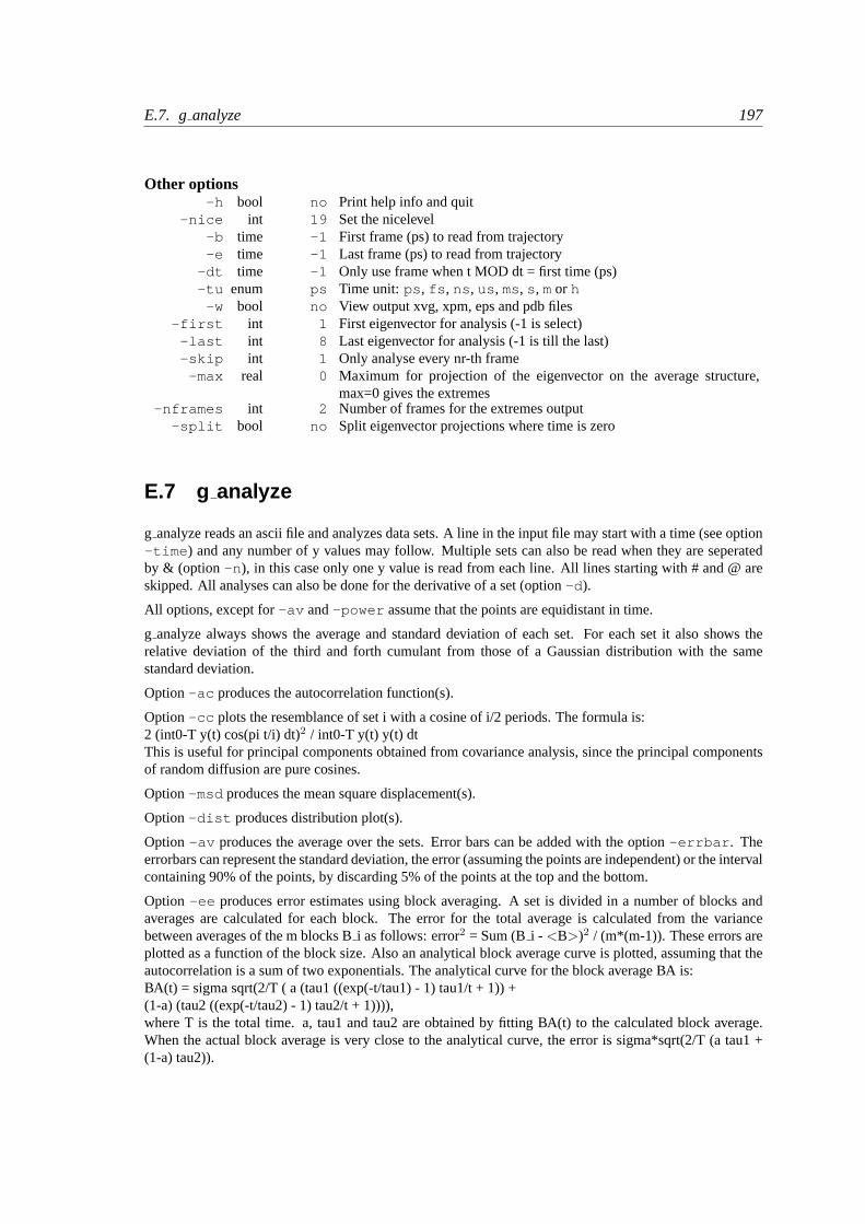
E.7. ganalyze 197
Other options-h bool no Print help info and quit
-nice int 19 Set the nicelevel-b time -1 First frame (ps) to read from trajectory-e time -1 Last frame (ps) to read from trajectory
-dt time -1 Only use frame when t MOD dt = first time (ps)-tu enum ps Time unit: ps , fs , ns , us , ms, s , mor h
-w bool no View output xvg, xpm, eps and pdb files-first int 1 First eigenvector for analysis (-1 is select)
-last int 8 Last eigenvector for analysis (-1 is till the last)-skip int 1 Only analyse every nr-th frame
-max real 0 Maximum for projection of the eigenvector on the average structure,max=0 gives the extremes
-nframes int 2 Number of frames for the extremes output-split bool no Split eigenvector projections where time is zero
E.7 g analyze
g analyze reads an ascii file and analyzes data sets. A line in the input file may start with a time (see option-time ) and any number of y values may follow. Multiple sets can also be read when they are seperatedby & (option -n ), in this case only one y value is read from each line. All lines starting with # and @ areskipped. All analyses can also be done for the derivative of a set (option-d ).
All options, except for-av and-power assume that the points are equidistant in time.
g analyze always shows the average and standard deviation of each set. For each set it also shows therelative deviation of the third and forth cumulant from those of a Gaussian distribution with the samestandard deviation.
Option-ac produces the autocorrelation function(s).
Option-cc plots the resemblance of set i with a cosine of i/2 periods. The formula is:2 (int0-T y(t) cos(pi t/i) dt)2 / int0-T y(t) y(t) dtThis is useful for principal components obtained from covariance analysis, since the principal componentsof random diffusion are pure cosines.
Option-msd produces the mean square displacement(s).
Option-dist produces distribution plot(s).
Option -av produces the average over the sets. Error bars can be added with the option-errbar . Theerrorbars can represent the standard deviation, the error (assuming the points are independent) or the intervalcontaining 90% of the points, by discarding 5% of the points at the top and the bottom.
Option -ee produces error estimates using block averaging. A set is divided in a number of blocks andaverages are calculated for each block. The error for the total average is calculated from the variancebetween averages of the m blocks Bi as follows: error2 = Sum (Bi - <B>)2 / (m*(m-1)). These errors areplotted as a function of the block size. Also an analytical block average curve is plotted, assuming that theautocorrelation is a sum of two exponentials. The analytical curve for the block average BA is:BA(t) = sigma sqrt(2/T ( a (tau1 ((exp(-t/tau1) - 1) tau1/t + 1)) +(1-a) (tau2 ((exp(-t/tau2) - 1) tau2/t + 1)))),where T is the total time. a, tau1 and tau2 are obtained by fitting BA(t) to the calculated block average.When the actual block average is very close to the analytical curve, the error is sigma*sqrt(2/T (a tau1 +(1-a) tau2)).
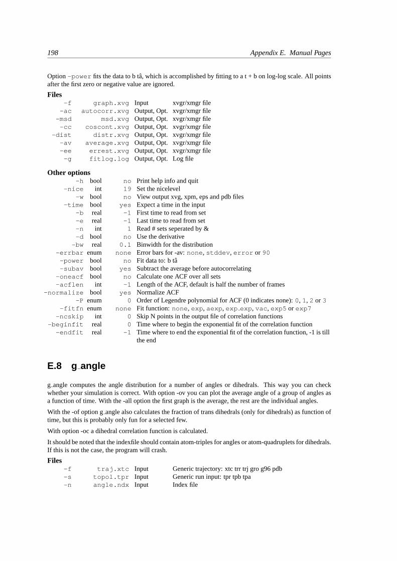
198 Appendix E. Manual Pages
Option-power fits the data to b ta, which is accomplished by fitting to a t + b on log-log scale. All pointsafter the first zero or negative value are ignored.
Files-f graph.xvg Input xvgr/xmgr file
-ac autocorr.xvg Output, Opt. xvgr/xmgr file-msd msd.xvg Output, Opt. xvgr/xmgr file
-cc coscont.xvg Output, Opt. xvgr/xmgr file-dist distr.xvg Output, Opt. xvgr/xmgr file
-av average.xvg Output, Opt. xvgr/xmgr file-ee errest.xvg Output, Opt. xvgr/xmgr file
-g fitlog.log Output, Opt. Log file
Other options-h bool no Print help info and quit
-nice int 19 Set the nicelevel-w bool no View output xvg, xpm, eps and pdb files
-time bool yes Expect a time in the input-b real -1 First time to read from set-e real -1 Last time to read from set-n int 1 Read # sets seperated by &-d bool no Use the derivative
-bw real 0.1 Binwidth for the distribution-errbar enum none Error bars for -av:none , stddev , error or 90
-power bool no Fit data to: b ta-subav bool yes Subtract the average before autocorrelating
-oneacf bool no Calculate one ACF over all sets-acflen int -1 Length of the ACF, default is half the number of frames
-normalize bool yes Normalize ACF-P enum 0 Order of Legendre polynomial for ACF (0 indicates none):0, 1, 2 or 3
-fitfn enum none Fit function: none , exp , aexp , exp exp , vac , exp5 or exp7-ncskip int 0 Skip N points in the output file of correlation functions
-beginfit real 0 Time where to begin the exponential fit of the correlation function-endfit real -1 Time where to end the exponential fit of the correlation function, -1 is till
the end
E.8 g angle
g angle computes the angle distribution for a number of angles or dihedrals. This way you can checkwhether your simulation is correct. With option -ov you can plot the average angle of a group of angles asa function of time. With the -all option the first graph is the average, the rest are the individual angles.
With the -of option gangle also calculates the fraction of trans dihedrals (only for dihedrals) as function oftime, but this is probably only fun for a selected few.
With option -oc a dihedral correlation function is calculated.
It should be noted that the indexfile should contain atom-triples for angles or atom-quadruplets for dihedrals.If this is not the case, the program will crash.
Files-f traj.xtc Input Generic trajectory: xtc trr trj gro g96 pdb-s topol.tpr Input Generic run input: tpr tpb tpa-n angle.ndx Input Index file
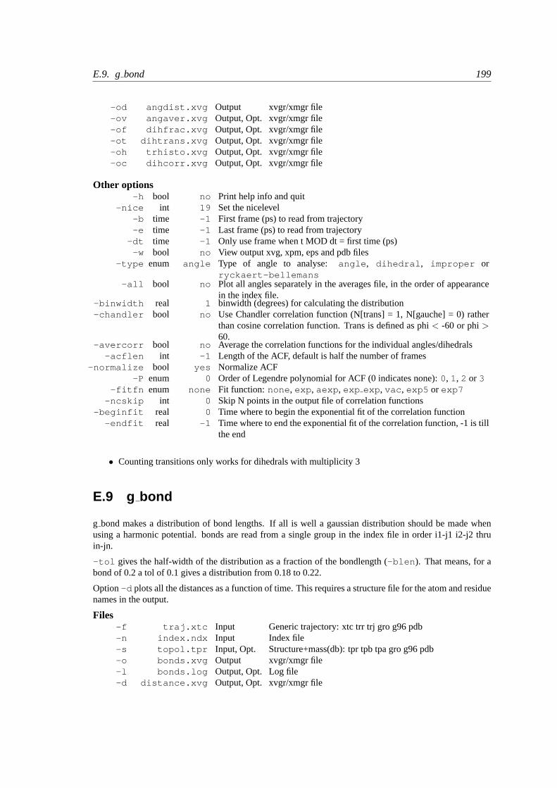
E.9. gbond 199
-od angdist.xvg Output xvgr/xmgr file-ov angaver.xvg Output, Opt. xvgr/xmgr file-of dihfrac.xvg Output, Opt. xvgr/xmgr file-ot dihtrans.xvg Output, Opt. xvgr/xmgr file-oh trhisto.xvg Output, Opt. xvgr/xmgr file-oc dihcorr.xvg Output, Opt. xvgr/xmgr file
Other options-h bool no Print help info and quit
-nice int 19 Set the nicelevel-b time -1 First frame (ps) to read from trajectory-e time -1 Last frame (ps) to read from trajectory
-dt time -1 Only use frame when t MOD dt = first time (ps)-w bool no View output xvg, xpm, eps and pdb files
-type enum angle Type of angle to analyse: angle , dihedral , improper orryckaert-bellemans
-all bool no Plot all angles separately in the averages file, in the order of appearancein the index file.
-binwidth real 1 binwidth (degrees) for calculating the distribution-chandler bool no Use Chandler correlation function (N[trans] = 1, N[gauche] = 0) rather
than cosine correlation function. Trans is defined as phi< -60 or phi>60.
-avercorr bool no Average the correlation functions for the individual angles/dihedrals-acflen int -1 Length of the ACF, default is half the number of frames
-normalize bool yes Normalize ACF-P enum 0 Order of Legendre polynomial for ACF (0 indicates none):0, 1, 2 or 3
-fitfn enum none Fit function: none , exp , aexp , exp exp , vac , exp5 or exp7-ncskip int 0 Skip N points in the output file of correlation functions
-beginfit real 0 Time where to begin the exponential fit of the correlation function-endfit real -1 Time where to end the exponential fit of the correlation function, -1 is till
the end
• Counting transitions only works for dihedrals with multiplicity 3
E.9 g bond
g bond makes a distribution of bond lengths. If all is well a gaussian distribution should be made whenusing a harmonic potential. bonds are read from a single group in the index file in order i1-j1 i2-j2 thruin-jn.
-tol gives the half-width of the distribution as a fraction of the bondlength (-blen ). That means, for abond of 0.2 a tol of 0.1 gives a distribution from 0.18 to 0.22.
Option-d plots all the distances as a function of time. This requires a structure file for the atom and residuenames in the output.
Files-f traj.xtc Input Generic trajectory: xtc trr trj gro g96 pdb-n index.ndx Input Index file-s topol.tpr Input, Opt. Structure+mass(db): tpr tpb tpa gro g96 pdb-o bonds.xvg Output xvgr/xmgr file-l bonds.log Output, Opt. Log file-d distance.xvg Output, Opt. xvgr/xmgr file
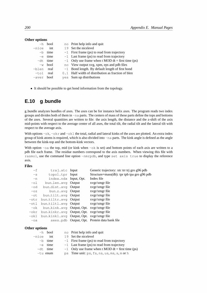
200 Appendix E. Manual Pages
Other options-h bool no Print help info and quit
-nice int 19 Set the nicelevel-b time -1 First frame (ps) to read from trajectory-e time -1 Last frame (ps) to read from trajectory
-dt time -1 Only use frame when t MOD dt = first time (ps)-w bool no View output xvg, xpm, eps and pdb files
-blen real -1 Bond length. By default length of first bond-tol real 0.1 Half width of distribution as fraction of blen
-aver bool yes Sum up distributions
• It should be possible to get bond information from the topology.
E.10 g bundle
g bundle analyzes bundles of axes. The axes can be for instance helix axes. The program reads two indexgroups and divides both of them in-na parts. The centers of mass of these parts define the tops and bottomsof the axes. Several quantities are written to file: the axis length, the distance and the z-shift of the axismid-points with respect to the average center of all axes, the total tilt, the radial tilt and the lateral tilt withrespect to the average axis.
With options-ok , -okr and-okl the total, radial and lateral kinks of the axes are plotted. An extra indexgroup of kink atoms is required, which is also divided into-na parts. The kink angle is defined as the anglebetween the kink-top and the bottom-kink vectors.
With option -oa the top, mid (or kink when-ok is set) and bottom points of each axis are written to apdb file each frame. The residue numbers correspond to the axis numbers. When viewing this file withrasmol , use the command line option-nmrpdb , and typeset axis true to display the referenceaxis.
Files-f traj.xtc Input Generic trajectory: xtc trr trj gro g96 pdb-s topol.tpr Input Structure+mass(db): tpr tpb tpa gro g96 pdb-n index.ndx Input, Opt. Index file
-ol bun len.xvg Output xvgr/xmgr file-od bun dist.xvg Output xvgr/xmgr file-oz bun z.xvg Output xvgr/xmgr file-ot bun tilt.xvg Output xvgr/xmgr file
-otr bun tiltr.xvg Output xvgr/xmgr file-otl bun tiltl.xvg Output xvgr/xmgr file
-ok bun kink.xvg Output, Opt. xvgr/xmgr file-okr bun kinkr.xvg Output, Opt. xvgr/xmgr file-okl bun kinkl.xvg Output, Opt. xvgr/xmgr file
-oa axes.pdb Output, Opt. Protein data bank file
Other options-h bool no Print help info and quit
-nice int 19 Set the nicelevel-b time -1 First frame (ps) to read from trajectory-e time -1 Last frame (ps) to read from trajectory
-dt time -1 Only use frame when t MOD dt = first time (ps)-tu enum ps Time unit: ps , fs , ns , us , ms, s , mor h
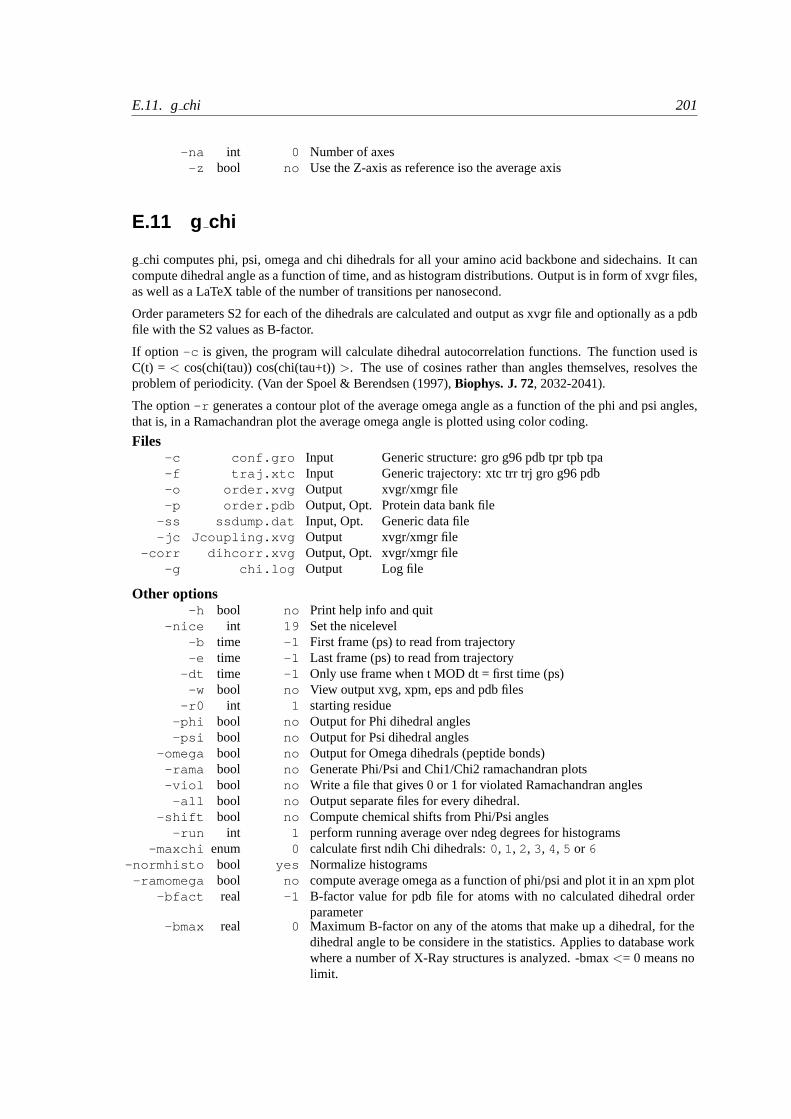
E.11. gchi 201
-na int 0 Number of axes-z bool no Use the Z-axis as reference iso the average axis
E.11 g chi
g chi computes phi, psi, omega and chi dihedrals for all your amino acid backbone and sidechains. It cancompute dihedral angle as a function of time, and as histogram distributions. Output is in form of xvgr files,as well as a LaTeX table of the number of transitions per nanosecond.
Order parameters S2 for each of the dihedrals are calculated and output as xvgr file and optionally as a pdbfile with the S2 values as B-factor.
If option -c is given, the program will calculate dihedral autocorrelation functions. The function used isC(t) = < cos(chi(tau)) cos(chi(tau+t))>. The use of cosines rather than angles themselves, resolves theproblem of periodicity. (Van der Spoel & Berendsen (1997),Biophys. J. 72, 2032-2041).
The option-r generates a contour plot of the average omega angle as a function of the phi and psi angles,that is, in a Ramachandran plot the average omega angle is plotted using color coding.
Files-c conf.gro Input Generic structure: gro g96 pdb tpr tpb tpa-f traj.xtc Input Generic trajectory: xtc trr trj gro g96 pdb-o order.xvg Output xvgr/xmgr file-p order.pdb Output, Opt. Protein data bank file
-ss ssdump.dat Input, Opt. Generic data file-jc Jcoupling.xvg Output xvgr/xmgr file
-corr dihcorr.xvg Output, Opt. xvgr/xmgr file-g chi.log Output Log file
Other options-h bool no Print help info and quit
-nice int 19 Set the nicelevel-b time -1 First frame (ps) to read from trajectory-e time -1 Last frame (ps) to read from trajectory
-dt time -1 Only use frame when t MOD dt = first time (ps)-w bool no View output xvg, xpm, eps and pdb files
-r0 int 1 starting residue-phi bool no Output for Phi dihedral angles-psi bool no Output for Psi dihedral angles
-omega bool no Output for Omega dihedrals (peptide bonds)-rama bool no Generate Phi/Psi and Chi1/Chi2 ramachandran plots-viol bool no Write a file that gives 0 or 1 for violated Ramachandran angles
-all bool no Output separate files for every dihedral.-shift bool no Compute chemical shifts from Phi/Psi angles
-run int 1 perform running average over ndeg degrees for histograms-maxchi enum 0 calculate first ndih Chi dihedrals:0, 1, 2, 3, 4, 5 or 6
-normhisto bool yes Normalize histograms-ramomega bool no compute average omega as a function of phi/psi and plot it in an xpm plot
-bfact real -1 B-factor value for pdb file for atoms with no calculated dihedral orderparameter
-bmax real 0 Maximum B-factor on any of the atoms that make up a dihedral, for thedihedral angle to be considere in the statistics. Applies to database workwhere a number of X-Ray structures is analyzed. -bmax<= 0 means nolimit.
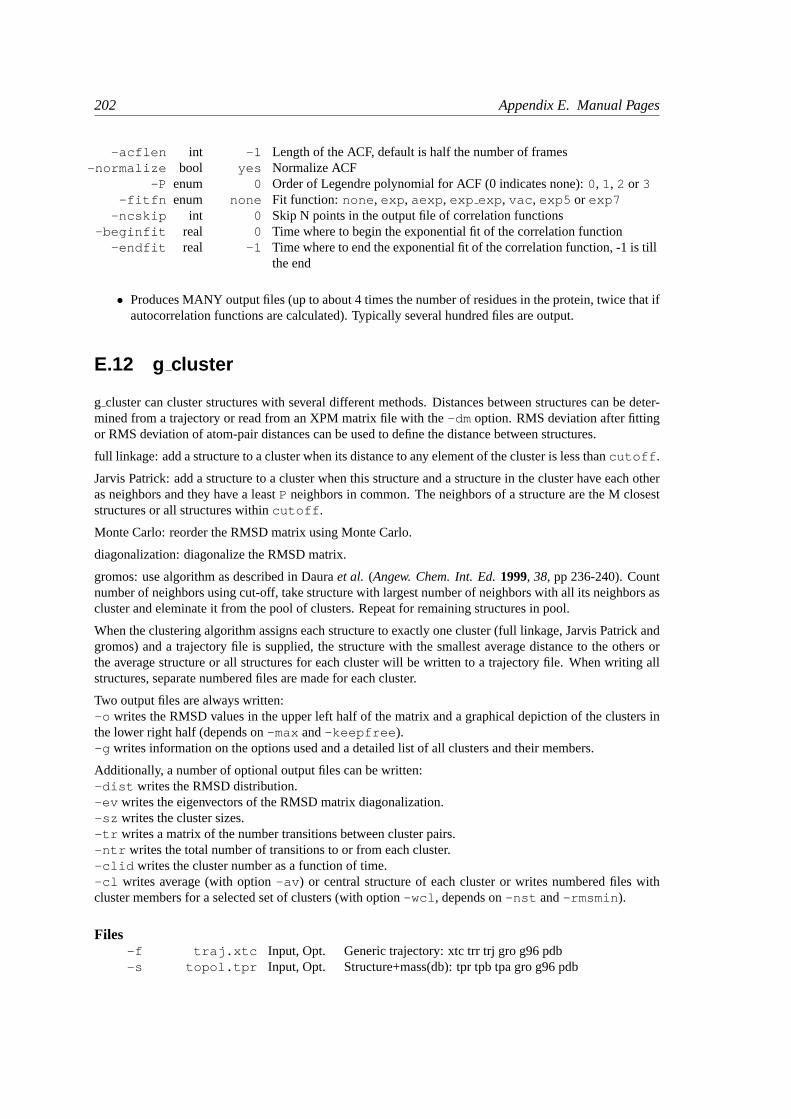
202 Appendix E. Manual Pages
-acflen int -1 Length of the ACF, default is half the number of frames-normalize bool yes Normalize ACF
-P enum 0 Order of Legendre polynomial for ACF (0 indicates none):0, 1, 2 or 3-fitfn enum none Fit function: none , exp , aexp , exp exp , vac , exp5 or exp7
-ncskip int 0 Skip N points in the output file of correlation functions-beginfit real 0 Time where to begin the exponential fit of the correlation function
-endfit real -1 Time where to end the exponential fit of the correlation function, -1 is tillthe end
• Produces MANY output files (up to about 4 times the number of residues in the protein, twice that ifautocorrelation functions are calculated). Typically several hundred files are output.
E.12 g cluster
g cluster can cluster structures with several different methods. Distances between structures can be deter-mined from a trajectory or read from an XPM matrix file with the-dm option. RMS deviation after fittingor RMS deviation of atom-pair distances can be used to define the distance between structures.
full linkage: add a structure to a cluster when its distance to any element of the cluster is less thancutoff .
Jarvis Patrick: add a structure to a cluster when this structure and a structure in the cluster have each otheras neighbors and they have a leastP neighbors in common. The neighbors of a structure are the M closeststructures or all structures withincutoff .
Monte Carlo: reorder the RMSD matrix using Monte Carlo.
diagonalization: diagonalize the RMSD matrix.
gromos: use algorithm as described in Dauraet al. (Angew. Chem. Int. Ed.1999, 38, pp 236-240). Countnumber of neighbors using cut-off, take structure with largest number of neighbors with all its neighbors ascluster and eleminate it from the pool of clusters. Repeat for remaining structures in pool.
When the clustering algorithm assigns each structure to exactly one cluster (full linkage, Jarvis Patrick andgromos) and a trajectory file is supplied, the structure with the smallest average distance to the others orthe average structure or all structures for each cluster will be written to a trajectory file. When writing allstructures, separate numbered files are made for each cluster.
Two output files are always written:-o writes the RMSD values in the upper left half of the matrix and a graphical depiction of the clusters inthe lower right half (depends on-max and-keepfree ).-g writes information on the options used and a detailed list of all clusters and their members.
Additionally, a number of optional output files can be written:-dist writes the RMSD distribution.-ev writes the eigenvectors of the RMSD matrix diagonalization.-sz writes the cluster sizes.-tr writes a matrix of the number transitions between cluster pairs.-ntr writes the total number of transitions to or from each cluster.-clid writes the cluster number as a function of time.-cl writes average (with option-av ) or central structure of each cluster or writes numbered files withcluster members for a selected set of clusters (with option-wcl , depends on-nst and-rmsmin ).
Files-f traj.xtc Input, Opt. Generic trajectory: xtc trr trj gro g96 pdb-s topol.tpr Input, Opt. Structure+mass(db): tpr tpb tpa gro g96 pdb
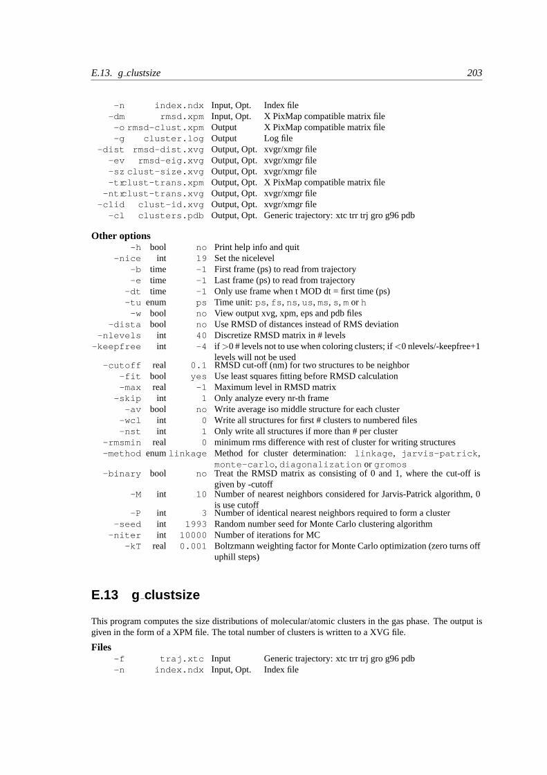
E.13. gclustsize 203
-n index.ndx Input, Opt. Index file-dm rmsd.xpm Input, Opt. X PixMap compatible matrix file
-o rmsd-clust.xpm Output X PixMap compatible matrix file-g cluster.log Output Log file
-dist rmsd-dist.xvg Output, Opt. xvgr/xmgr file-ev rmsd-eig.xvg Output, Opt. xvgr/xmgr file-sz clust-size.xvg Output, Opt. xvgr/xmgr file-trclust-trans.xpm Output, Opt. X PixMap compatible matrix file
-ntrclust-trans.xvg Output, Opt. xvgr/xmgr file-clid clust-id.xvg Output, Opt. xvgr/xmgr file
-cl clusters.pdb Output, Opt. Generic trajectory: xtc trr trj gro g96 pdb
Other options-h bool no Print help info and quit
-nice int 19 Set the nicelevel-b time -1 First frame (ps) to read from trajectory-e time -1 Last frame (ps) to read from trajectory
-dt time -1 Only use frame when t MOD dt = first time (ps)-tu enum ps Time unit: ps , fs , ns , us , ms, s , mor h
-w bool no View output xvg, xpm, eps and pdb files-dista bool no Use RMSD of distances instead of RMS deviation
-nlevels int 40 Discretize RMSD matrix in # levels-keepfree int -4 if >0 # levels not to use when coloring clusters; if<0 nlevels/-keepfree+1
levels will not be used-cutoff real 0.1 RMSD cut-off (nm) for two structures to be neighbor
-fit bool yes Use least squares fitting before RMSD calculation-max real -1 Maximum level in RMSD matrix
-skip int 1 Only analyze every nr-th frame-av bool no Write average iso middle structure for each cluster
-wcl int 0 Write all structures for first # clusters to numbered files-nst int 1 Only write all structures if more than # per cluster
-rmsmin real 0 minimum rms difference with rest of cluster for writing structures-method enumlinkage Method for cluster determination:linkage , jarvis-patrick ,
monte-carlo , diagonalization or gromos-binary bool no Treat the RMSD matrix as consisting of 0 and 1, where the cut-off is
given by -cutoff-M int 10 Number of nearest neighbors considered for Jarvis-Patrick algorithm, 0
is use cutoff-P int 3 Number of identical nearest neighbors required to form a cluster
-seed int 1993 Random number seed for Monte Carlo clustering algorithm-niter int 10000 Number of iterations for MC
-kT real 0.001 Boltzmann weighting factor for Monte Carlo optimization (zero turns offuphill steps)
E.13 g clustsize
This program computes the size distributions of molecular/atomic clusters in the gas phase. The output isgiven in the form of a XPM file. The total number of clusters is written to a XVG file.
Files-f traj.xtc Input Generic trajectory: xtc trr trj gro g96 pdb-n index.ndx Input, Opt. Index file
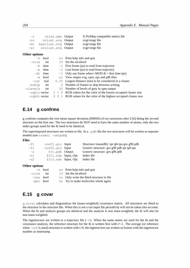
204 Appendix E. Manual Pages
-o csize.xpm Output X PixMap compatible matrix file-nc nclust.xvg Output xvgr/xmgr file-mc maxclust.xvg Output xvgr/xmgr file-ac avclust.xvg Output xvgr/xmgr file
Other options-h bool no Print help info and quit
-nice int 19 Set the nicelevel-b time -1 First frame (ps) to read from trajectory-e time -1 Last frame (ps) to read from trajectory
-dt time -1 Only use frame when t MOD dt = first time (ps)-w bool no View output xvg, xpm, eps and pdb files
-cut real 0.35 Largest distance (nm) to be considered in a cluster-nskip int 0 Number of frames to skip between writing
-nlevels int 20 Number of levels of grey in xpm output-rgblo vector 1 1 0 RGB values for the color of the lowest occupied cluster size-rgbhi vector 0 0 1 RGB values for the color of the highest occupied cluster size
E.14 g confrms
g confrms computes the root mean square deviation (RMSD) of two structures after LSQ fitting the secondstructure on the first one. The two structures do NOT need to have the same number of atoms, only the twoindex groups used for the fit need to be identical.
The superimposed structures are written to file. In a.pdb file the two structures will be written as separatemodels (userasmol -nmrpdb ).
Files-f1 conf1.gro Input Structure+mass(db): tpr tpb tpa gro g96 pdb-f2 conf2.gro Input Generic structure: gro g96 pdb tpr tpb tpa
-o fit.pdb Output Generic structure: gro g96 pdb-n1 fit1.ndx Input, Opt. Index file-n2 fit2.ndx Input, Opt. Index file
Other options-h bool no Print help info and quit
-nice int 19 Set the nicelevel-one bool no Only write the fitted structure to file-pbc bool no Try to make molecules whole again
E.15 g covar
g covar calculates and diagonalizes the (mass-weighted) covariance matrix. All structures are fitted tothe structure in the structure file. When this is not a run input file periodicity will not be taken into account.When the fit and analysis groups are identical and the analysis is non mass-weighted, the fit will also benon mass-weighted.
The eigenvectors are written to a trajectory file (-v ). When the same atoms are used for the fit and thecovariance analysis, the reference structure for the fit is written first with t=-1. The average (or referencewhen-ref is used) structure is written with t=0, the eigenvectors are written as frames with the eigenvectornumber as timestamp.
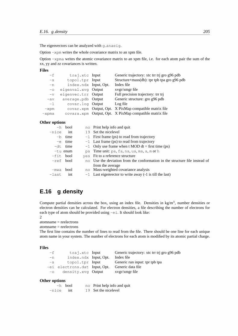
E.16. gdensity 205
The eigenvectors can be analyzed withg anaeig .
Option-xpm writes the whole covariance matrix to an xpm file.
Option -xpma writes the atomic covariance matrix to an xpm file, i.e. for each atom pair the sum of thexx, yy and zz covariances is written.
Files-f traj.xtc Input Generic trajectory: xtc trr trj gro g96 pdb-s topol.tpr Input Structure+mass(db): tpr tpb tpa gro g96 pdb-n index.ndx Input, Opt. Index file-o eigenval.xvg Output xvgr/xmgr file-v eigenvec.trr Output Full precision trajectory: trr trj
-av average.pdb Output Generic structure: gro g96 pdb-l covar.log Output Log file
-xpm covar.xpm Output, Opt. X PixMap compatible matrix file-xpma covara.xpm Output, Opt. X PixMap compatible matrix file
Other options-h bool no Print help info and quit
-nice int 19 Set the nicelevel-b time -1 First frame (ps) to read from trajectory-e time -1 Last frame (ps) to read from trajectory
-dt time -1 Only use frame when t MOD dt = first time (ps)-tu enum ps Time unit: ps , fs , ns , us , ms, s , mor h
-fit bool yes Fit to a reference structure-ref bool no Use the deviation from the conformation in the structure file instead of
from the average-mwa bool no Mass-weighted covariance analysis
-last int -1 Last eigenvector to write away (-1 is till the last)
E.16 g density
Compute partial densities across the box, using an index file. Densities in kg/m3, number densities orelectron densities can be calculated. For electron densities, a file describing the number of electrons foreach type of atom should be provided using-ei . It should look like:2atomname = nrelectronsatomname = nrelectronsThe first line contains the number of lines to read from the file. There should be one line for each uniqueatom name in your system. The number of electrons for each atom is modified by its atomic partial charge.
Files-f traj.xtc Input Generic trajectory: xtc trr trj gro g96 pdb-n index.ndx Input, Opt. Index file-s topol.tpr Input Generic run input: tpr tpb tpa
-ei electrons.dat Input, Opt. Generic data file-o density.xvg Output xvgr/xmgr file
Other options-h bool no Print help info and quit
-nice int 19 Set the nicelevel
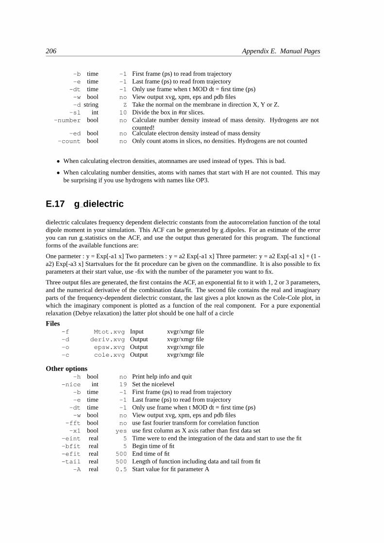
206 Appendix E. Manual Pages
-b time -1 First frame (ps) to read from trajectory-e time -1 Last frame (ps) to read from trajectory
-dt time -1 Only use frame when t MOD dt = first time (ps)-w bool no View output xvg, xpm, eps and pdb files-d string Z Take the normal on the membrane in direction X, Y or Z.
-sl int 10 Divide the box in #nr slices.-number bool no Calculate number density instead of mass density. Hydrogens are not
counted!-ed bool no Calculate electron density instead of mass density
-count bool no Only count atoms in slices, no densities. Hydrogens are not counted
• When calculating electron densities, atomnames are used instead of types. This is bad.
• When calculating number densities, atoms with names that start with H are not counted. This maybe surprising if you use hydrogens with names like OP3.
E.17 g dielectric
dielectric calculates frequency dependent dielectric constants from the autocorrelation function of the totaldipole moment in your simulation. This ACF can be generated by gdipoles. For an estimate of the erroryou can run gstatistics on the ACF, and use the output thus generated for this program. The functionalforms of the available functions are:
One parmeter : y = Exp[-a1 x] Two parmeters : y = a2 Exp[-a1 x] Three parmeter: y = a2 Exp[-a1 x] + (1 -a2) Exp[-a3 x] Startvalues for the fit procedure can be given on the commandline. It is also possible to fixparameters at their start value, use -fix with the number of the parameter you want to fix.
Three output files are generated, the first contains the ACF, an exponential fit to it with 1, 2 or 3 parameters,and the numerical derivative of the combination data/fit. The second file contains the real and imaginaryparts of the frequency-dependent dielectric constant, the last gives a plot known as the Cole-Cole plot, inwhich the imaginary component is plotted as a function of the real component. For a pure exponentialrelaxation (Debye relaxation) the latter plot should be one half of a circle
Files-f Mtot.xvg Input xvgr/xmgr file-d deriv.xvg Output xvgr/xmgr file-o epsw.xvg Output xvgr/xmgr file-c cole.xvg Output xvgr/xmgr file
Other options-h bool no Print help info and quit
-nice int 19 Set the nicelevel-b time -1 First frame (ps) to read from trajectory-e time -1 Last frame (ps) to read from trajectory
-dt time -1 Only use frame when t MOD dt = first time (ps)-w bool no View output xvg, xpm, eps and pdb files
-fft bool no use fast fourier transform for correlation function-x1 bool yes use first column as X axis rather than first data set
-eint real 5 Time were to end the integration of the data and start to use the fit-bfit real 5 Begin time of fit-efit real 500 End time of fit-tail real 500 Length of function including data and tail from fit
-A real 0.5 Start value for fit parameter A
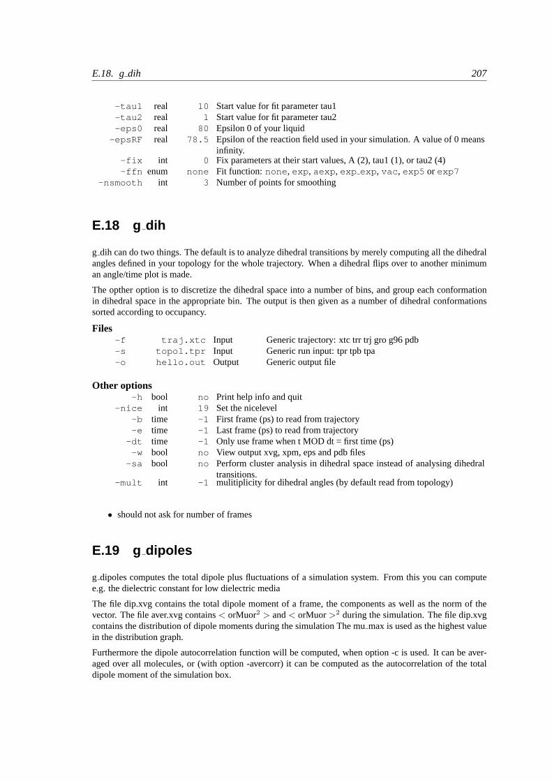
E.18. gdih 207
-tau1 real 10 Start value for fit parameter tau1-tau2 real 1 Start value for fit parameter tau2-eps0 real 80 Epsilon 0 of your liquid
-epsRF real 78.5 Epsilon of the reaction field used in your simulation. A value of 0 meansinfinity.
-fix int 0 Fix parameters at their start values, A (2), tau1 (1), or tau2 (4)-ffn enum none Fit function: none , exp , aexp , exp exp , vac , exp5 or exp7
-nsmooth int 3 Number of points for smoothing
E.18 g dih
g dih can do two things. The default is to analyze dihedral transitions by merely computing all the dihedralangles defined in your topology for the whole trajectory. When a dihedral flips over to another minimuman angle/time plot is made.
The opther option is to discretize the dihedral space into a number of bins, and group each conformationin dihedral space in the appropriate bin. The output is then given as a number of dihedral conformationssorted according to occupancy.
Files-f traj.xtc Input Generic trajectory: xtc trr trj gro g96 pdb-s topol.tpr Input Generic run input: tpr tpb tpa-o hello.out Output Generic output file
Other options-h bool no Print help info and quit
-nice int 19 Set the nicelevel-b time -1 First frame (ps) to read from trajectory-e time -1 Last frame (ps) to read from trajectory
-dt time -1 Only use frame when t MOD dt = first time (ps)-w bool no View output xvg, xpm, eps and pdb files
-sa bool no Perform cluster analysis in dihedral space instead of analysing dihedraltransitions.
-mult int -1 mulitiplicity for dihedral angles (by default read from topology)
• should not ask for number of frames
E.19 g dipoles
g dipoles computes the total dipole plus fluctuations of a simulation system. From this you can computee.g. the dielectric constant for low dielectric media
The file dip.xvg contains the total dipole moment of a frame, the components as well as the norm of thevector. The file aver.xvg contains< orMuor2 > and< orMuor>2 during the simulation. The file dip.xvgcontains the distribution of dipole moments during the simulation The mumax is used as the highest valuein the distribution graph.
Furthermore the dipole autocorrelation function will be computed, when option -c is used. It can be aver-aged over all molecules, or (with option -avercorr) it can be computed as the autocorrelation of the totaldipole moment of the simulation box.
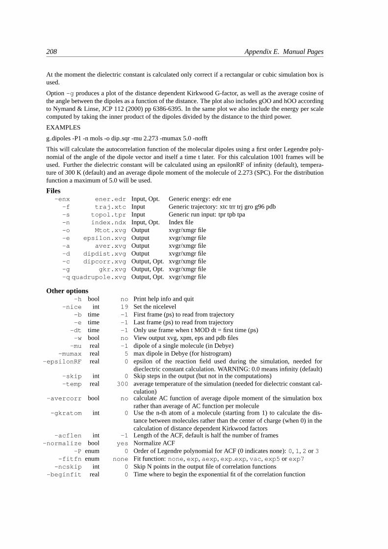
208 Appendix E. Manual Pages
At the moment the dielectric constant is calculated only correct if a rectangular or cubic simulation box isused.
Option -g produces a plot of the distance dependent Kirkwood G-factor, as well as the average cosine ofthe angle between the dipoles as a function of the distance. The plot also includes gOO and hOO accordingto Nymand & Linse, JCP 112 (2000) pp 6386-6395. In the same plot we also include the energy per scalecomputed by taking the inner product of the dipoles divided by the distance to the third power.
EXAMPLES
g dipoles -P1 -n mols -o dipsqr -mu 2.273 -mumax 5.0 -nofft
This will calculate the autocorrelation function of the molecular dipoles using a first order Legendre poly-nomial of the angle of the dipole vector and itself a time t later. For this calculation 1001 frames will beused. Further the dielectric constant will be calculated using an epsilonRF of infinity (default), tempera-ture of 300 K (default) and an average dipole moment of the molecule of 2.273 (SPC). For the distributionfunction a maximum of 5.0 will be used.
Files-enx ener.edr Input, Opt. Generic energy: edr ene
-f traj.xtc Input Generic trajectory: xtc trr trj gro g96 pdb-s topol.tpr Input Generic run input: tpr tpb tpa-n index.ndx Input, Opt. Index file-o Mtot.xvg Output xvgr/xmgr file-e epsilon.xvg Output xvgr/xmgr file-a aver.xvg Output xvgr/xmgr file-d dipdist.xvg Output xvgr/xmgr file-c dipcorr.xvg Output, Opt. xvgr/xmgr file-g gkr.xvg Output, Opt. xvgr/xmgr file-q quadrupole.xvg Output, Opt. xvgr/xmgr file
Other options-h bool no Print help info and quit
-nice int 19 Set the nicelevel-b time -1 First frame (ps) to read from trajectory-e time -1 Last frame (ps) to read from trajectory
-dt time -1 Only use frame when t MOD dt = first time (ps)-w bool no View output xvg, xpm, eps and pdb files
-mu real -1 dipole of a single molecule (in Debye)-mumax real 5 max dipole in Debye (for histrogram)
-epsilonRF real 0 epsilon of the reaction field used during the simulation, needed fordieclectric constant calculation. WARNING: 0.0 means infinity (default)
-skip int 0 Skip steps in the output (but not in the computations)-temp real 300 average temperature of the simulation (needed for dielectric constant cal-
culation)-avercorr bool no calculate AC function of average dipole moment of the simulation box
rather than average of AC function per molecule-gkratom int 0 Use the n-th atom of a molecule (starting from 1) to calculate the dis-
tance between molecules rather than the center of charge (when 0) in thecalculation of distance dependent Kirkwood factors
-acflen int -1 Length of the ACF, default is half the number of frames-normalize bool yes Normalize ACF
-P enum 0 Order of Legendre polynomial for ACF (0 indicates none):0, 1, 2 or 3-fitfn enum none Fit function: none , exp , aexp , exp exp , vac , exp5 or exp7
-ncskip int 0 Skip N points in the output file of correlation functions-beginfit real 0 Time where to begin the exponential fit of the correlation function
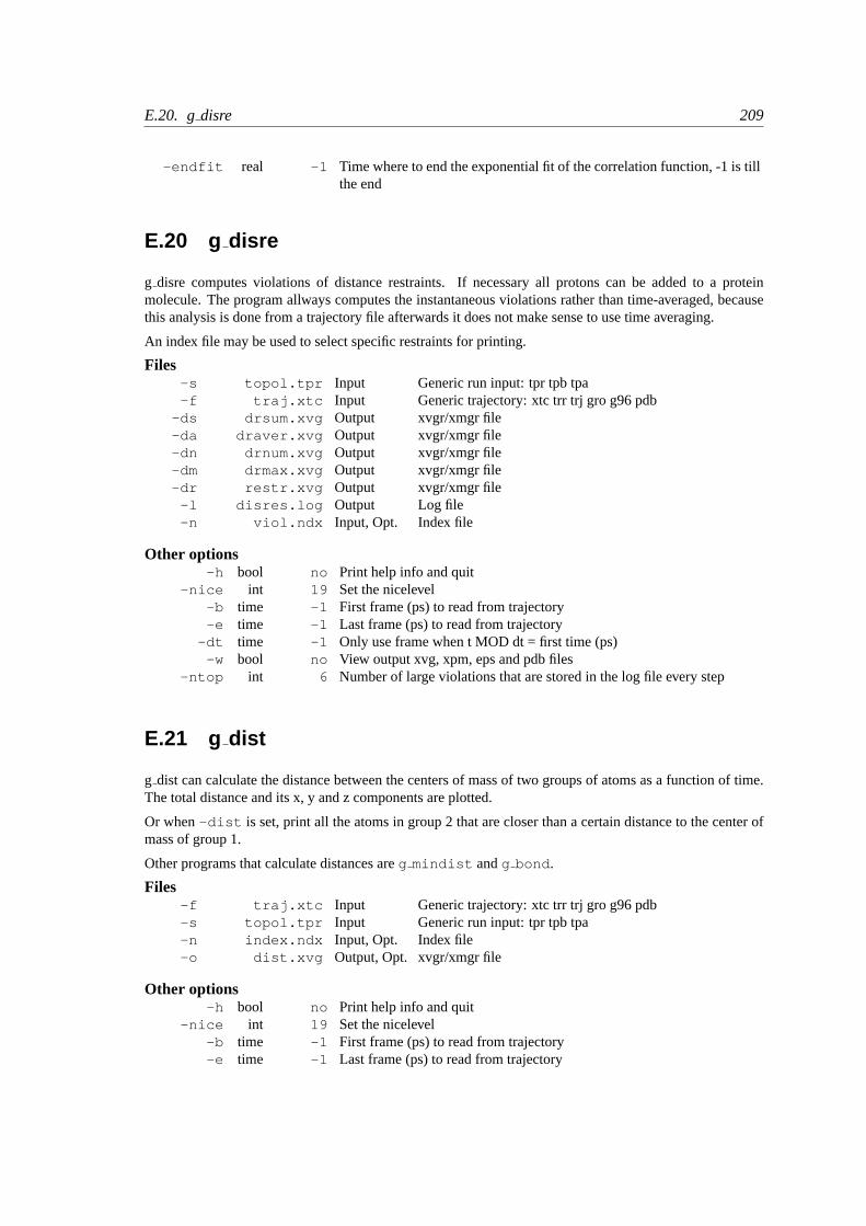
E.20. gdisre 209
-endfit real -1 Time where to end the exponential fit of the correlation function, -1 is tillthe end
E.20 g disre
g disre computes violations of distance restraints. If necessary all protons can be added to a proteinmolecule. The program allways computes the instantaneous violations rather than time-averaged, becausethis analysis is done from a trajectory file afterwards it does not make sense to use time averaging.
An index file may be used to select specific restraints for printing.
Files-s topol.tpr Input Generic run input: tpr tpb tpa-f traj.xtc Input Generic trajectory: xtc trr trj gro g96 pdb
-ds drsum.xvg Output xvgr/xmgr file-da draver.xvg Output xvgr/xmgr file-dn drnum.xvg Output xvgr/xmgr file-dm drmax.xvg Output xvgr/xmgr file-dr restr.xvg Output xvgr/xmgr file
-l disres.log Output Log file-n viol.ndx Input, Opt. Index file
Other options-h bool no Print help info and quit
-nice int 19 Set the nicelevel-b time -1 First frame (ps) to read from trajectory-e time -1 Last frame (ps) to read from trajectory
-dt time -1 Only use frame when t MOD dt = first time (ps)-w bool no View output xvg, xpm, eps and pdb files
-ntop int 6 Number of large violations that are stored in the log file every step
E.21 g dist
g dist can calculate the distance between the centers of mass of two groups of atoms as a function of time.The total distance and its x, y and z components are plotted.
Or when-dist is set, print all the atoms in group 2 that are closer than a certain distance to the center ofmass of group 1.
Other programs that calculate distances areg mindist andg bond .
Files-f traj.xtc Input Generic trajectory: xtc trr trj gro g96 pdb-s topol.tpr Input Generic run input: tpr tpb tpa-n index.ndx Input, Opt. Index file-o dist.xvg Output, Opt. xvgr/xmgr file
Other options-h bool no Print help info and quit
-nice int 19 Set the nicelevel-b time -1 First frame (ps) to read from trajectory-e time -1 Last frame (ps) to read from trajectory
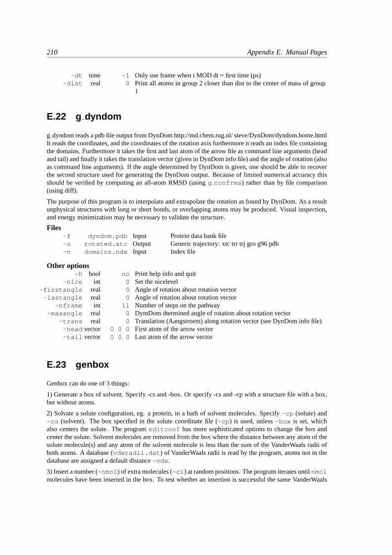
210 Appendix E. Manual Pages
-dt time -1 Only use frame when t MOD dt = first time (ps)-dist real 0 Print all atoms in group 2 closer than dist to the center of mass of group
1
E.22 g dyndom
g dyndom reads a pdb file output from DynDom http://md.chem.rug.nl/ steve/DynDom/dyndom.home.htmlIt reads the coordinates, and the coordinates of the rotation axis furthermore it reads an index file containingthe domains. Furthermore it takes the first and last atom of the arrow file as command line arguments (headand tail) and finally it takes the translation vector (given in DynDom info file) and the angle of rotation (alsoas command line arguments). If the angle determined by DynDom is given, one should be able to recoverthe second structure used for generating the DynDom output. Because of limited numerical accuracy thisshould be verified by computing an all-atom RMSD (usingg confrms ) rather than by file comparison(using diff).
The purpose of this program is to interpolate and extrapolate the rotation as found by DynDom. As a resultunphysical structures with long or short bonds, or overlapping atoms may be produced. Visual inspection,and energy minimization may be necessary to validate the structure.
Files-f dyndom.pdb Input Protein data bank file-o rotated.xtc Output Generic trajectory: xtc trr trj gro g96 pdb-n domains.ndx Input Index file
Other options-h bool no Print help info and quit
-nice int 0 Set the nicelevel-firstangle real 0 Angle of rotation about rotation vector
-lastangle real 0 Angle of rotation about rotation vector-nframe int 11 Number of steps on the pathway
-maxangle real 0 DymDom dtermined angle of rotation about rotation vector-trans real 0 Translation (Aangstroem) along rotation vector (see DynDom info file)
-head vector 0 0 0 First atom of the arrow vector-tail vector 0 0 0 Last atom of the arrow vector
E.23 genbox
Genbox can do one of 3 things:
1) Generate a box of solvent. Specify -cs and -box. Or specify -cs and -cp with a structure file with a box,but without atoms.
2) Solvate a solute configuration, eg. a protein, in a bath of solvent molecules. Specify-cp (solute) and-cs (solvent). The box specified in the solute coordinate file (-cp ) is used, unless-box is set, whichalso centers the solute. The programeditconf has more sophisticated options to change the box andcenter the solute. Solvent molecules are removed from the box where the distance between any atom of thesolute molecule(s) and any atom of the solvent molecule is less than the sum of the VanderWaals radii ofboth atoms. A database (vdwradii.dat ) of VanderWaals radii is read by the program, atoms not in thedatabase are assigned a default distance-vdw .
3) Insert a number (-nmol ) of extra molecules (-ci ) at random positions. The program iterates untilnmolmolecules have been inserted in the box. To test whether an insertion is successful the same VanderWaals
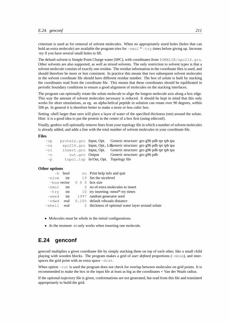
E.24. genconf 211
criterium is used as for removal of solvent molecules. When no appropriately sized holes (holes that canhold an extra molecule) are available the program tries for-nmol * -try times before giving up. Increase-try if you have several small holes to fill.
The default solvent is Simple Point Charge water (SPC), with coordinates from$GMXLIB/spc216.gro .Other solvents are also supported, as well as mixed solvents. The only restriction to solvent types is that asolvent molecule consists of exactly one residue. The residue information in the coordinate files is used, andshould therefore be more or less consistent. In practice this means that two subsequent solvent moleculesin the solvent coordinate file should have different residue number. The box of solute is built by stackingthe coordinates read from the coordinate file. This means that these coordinates should be equlibrated inperiodic boundary conditions to ensure a good alignment of molecules on the stacking interfaces.
The program can optionally rotate the solute molecule to align the longest molecule axis along a box edge.This way the amount of solvent molecules necessary is reduced. It should be kept in mind that this onlyworks for short simulations, as eg. an alpha-helical peptide in solution can rotate over 90 degrees, within500 ps. In general it is therefore better to make a more or less cubic box.
Setting -shell larger than zero will place a layer of water of the specified thickness (nm) around the solute.Hint: it is a good idea to put the protein in the center of a box first (using editconf).
Finally, genbox will optionally remove lines from your topology file in which a number of solvent moleculesis already added, and adds a line with the total number of solvent molecules in your coordinate file.
Files-cp protein.gro Input, Opt. Generic structure: gro g96 pdb tpr tpb tpa-cs spc216.gro Input, Opt., Lib.Generic structure: gro g96 pdb tpr tpb tpa-ci insert.gro Input, Opt. Generic structure: gro g96 pdb tpr tpb tpa
-o out.gro Output Generic structure: gro g96 pdb-p topol.top In/Out, Opt. Topology file
Other options-h bool no Print help info and quit
-nice int 19 Set the nicelevel-box vector 0 0 0 box size
-nmol int 0 no of extra molecules to insert-try int 10 try inserting -nmol*-try times
-seed int 1997 random generator seed-vdwd real 0.105 default vdwaals distance
-shell real 0 thickness of optional water layer around solute
• Molecules must be whole in the initial configurations.
• At the moment -ci only works when inserting one molecule.
E.24 genconf
genconf multiplies a given coordinate file by simply stacking them on top of each other, like a small childplaying with wooden blocks. The program makes a grid ofuser definedproportions (-nbox ), and inter-spaces the grid point with an extra space-dist .
When option-rot is used the program does not check for overlap between molecules on grid points. It isrecommended to make the box in the input file at least as big as the coordinates + Van der Waals radius.
If the optional trajectory file is given, conformations are not generated, but read from this file and translatedappropriately to build the grid.
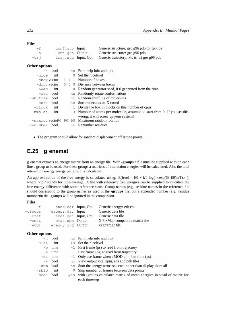
212 Appendix E. Manual Pages
Files-f conf.gro Input Generic structure: gro g96 pdb tpr tpb tpa-o out.gro Output Generic structure: gro g96 pdb
-trj traj.xtc Input, Opt. Generic trajectory: xtc trr trj gro g96 pdb
Other options-h bool no Print help info and quit
-nice int 0 Set the nicelevel-nbox vector 1 1 1 Number of boxes-dist vector 0 0 0 Distance between boxes-seed int 0 Random generator seed, if 0 generated from the time
-rot bool no Randomly rotate conformations-shuffle bool no Random shuffling of molecules
-sort bool no Sort molecules on X coord-block int 1 Divide the box in blocks on this number of cpus
-nmolat int 3 Number of atoms per molecule, assumed to start from 0. If you set thiswrong, it will screw up your system!
-maxrot vector90 90 90 Maximum random rotation-renumber bool no Renumber residues
• The program should allow for random displacement off lattice points.
E.25 g enemat
g enemat extracts an energy matrix from an energy file. With-groups a file must be supplied with on eachline a group to be used. For these groups a matrices of interaction energies will be calculated. Also the totalinteraction energy energy per group is calculated.
An approximation of the free energy is calculated using: E(free) = E0 + kT log(<exp((E-E0)/kT)> ),where ’<>’ stands for time-average. A file with reference free energies can be supplied to calculate thefree energy difference with some reference state. Group names (e.g. residue names in the reference fileshould correspond to the group names as used in the-groups file, but a appended number (e.g. residuenumber)in the-groupswill be ignored in the comparison.
Files-f ener.edr Input, Opt. Generic energy: edr ene
-groups groups.dat Input Generic data file-eref eref.dat Input, Opt. Generic data file-emat emat.xpm Output X PixMap compatible matrix file-etot energy.xvg Output xvgr/xmgr file
Other options-h bool no Print help info and quit
-nice int 19 Set the nicelevel-b time -1 First frame (ps) to read from trajectory-e time -1 Last frame (ps) to read from trajectory
-dt time -1 Only use frame when t MOD dt = first time (ps)-w bool no View output xvg, xpm, eps and pdb files
-sum bool no Sum the energy terms selected rather than display them all-skip int 0 Skip number of frames between data points-mean bool yes with -groups calculates matrix of mean energies in stead of matrix for
each timestep
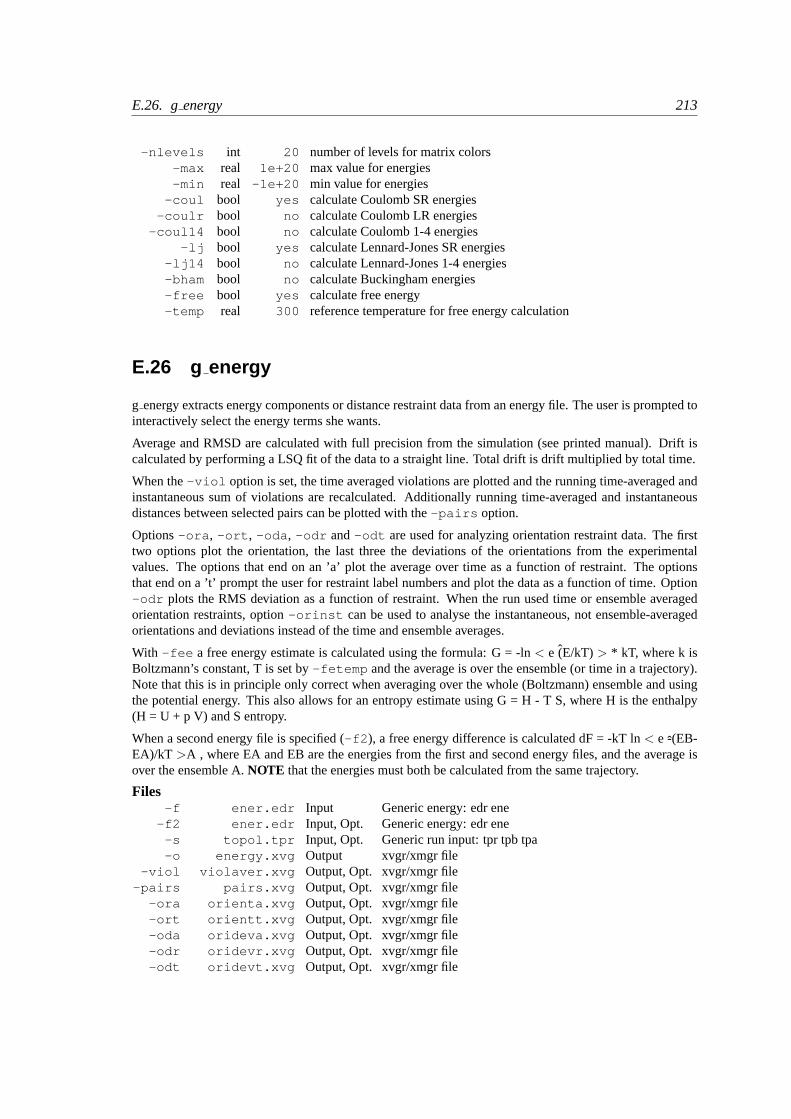
E.26. genergy 213
-nlevels int 20 number of levels for matrix colors-max real 1e+20 max value for energies-min real -1e+20 min value for energies
-coul bool yes calculate Coulomb SR energies-coulr bool no calculate Coulomb LR energies
-coul14 bool no calculate Coulomb 1-4 energies-lj bool yes calculate Lennard-Jones SR energies
-lj14 bool no calculate Lennard-Jones 1-4 energies-bham bool no calculate Buckingham energies-free bool yes calculate free energy-temp real 300 reference temperature for free energy calculation
E.26 g energy
g energy extracts energy components or distance restraint data from an energy file. The user is prompted tointeractively select the energy terms she wants.
Average and RMSD are calculated with full precision from the simulation (see printed manual). Drift iscalculated by performing a LSQ fit of the data to a straight line. Total drift is drift multiplied by total time.
When the-viol option is set, the time averaged violations are plotted and the running time-averaged andinstantaneous sum of violations are recalculated. Additionally running time-averaged and instantaneousdistances between selected pairs can be plotted with the-pairs option.
Options-ora , -ort , -oda , -odr and-odt are used for analyzing orientation restraint data. The firsttwo options plot the orientation, the last three the deviations of the orientations from the experimentalvalues. The options that end on an ’a’ plot the average over time as a function of restraint. The optionsthat end on a ’t’ prompt the user for restraint label numbers and plot the data as a function of time. Option-odr plots the RMS deviation as a function of restraint. When the run used time or ensemble averagedorientation restraints, option-orinst can be used to analyse the instantaneous, not ensemble-averagedorientations and deviations instead of the time and ensemble averages.
With -fee a free energy estimate is calculated using the formula: G = -ln< e (E/kT)> * kT, where k isBoltzmann’s constant, T is set by-fetemp and the average is over the ensemble (or time in a trajectory).Note that this is in principle only correct when averaging over the whole (Boltzmann) ensemble and usingthe potential energy. This also allows for an entropy estimate using G = H - T S, where H is the enthalpy(H = U + p V) and S entropy.
When a second energy file is specified (-f2 ), a free energy difference is calculated dF = -kT ln< e -(EB-EA)/kT >A , where EA and EB are the energies from the first and second energy files, and the average isover the ensemble A.NOTE that the energies must both be calculated from the same trajectory.
Files-f ener.edr Input Generic energy: edr ene
-f2 ener.edr Input, Opt. Generic energy: edr ene-s topol.tpr Input, Opt. Generic run input: tpr tpb tpa-o energy.xvg Output xvgr/xmgr file
-viol violaver.xvg Output, Opt. xvgr/xmgr file-pairs pairs.xvg Output, Opt. xvgr/xmgr file
-ora orienta.xvg Output, Opt. xvgr/xmgr file-ort orientt.xvg Output, Opt. xvgr/xmgr file-oda orideva.xvg Output, Opt. xvgr/xmgr file-odr oridevr.xvg Output, Opt. xvgr/xmgr file-odt oridevt.xvg Output, Opt. xvgr/xmgr file
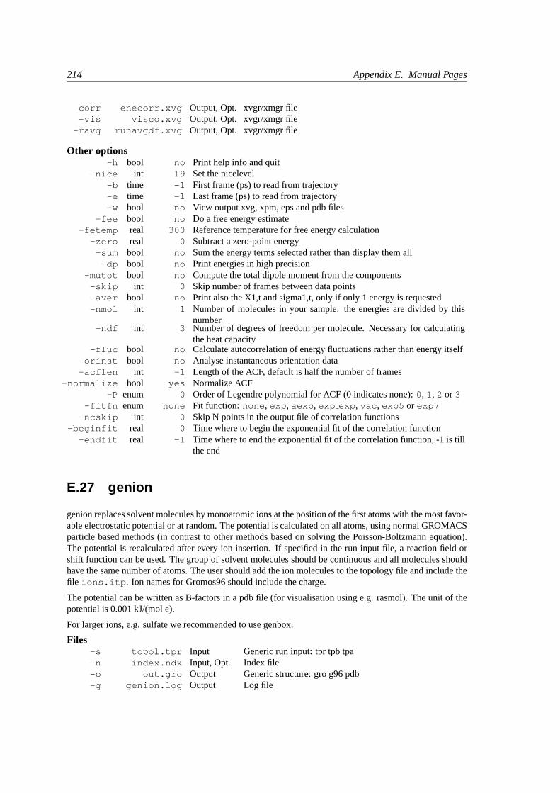
214 Appendix E. Manual Pages
-corr enecorr.xvg Output, Opt. xvgr/xmgr file-vis visco.xvg Output, Opt. xvgr/xmgr file
-ravg runavgdf.xvg Output, Opt. xvgr/xmgr file
Other options-h bool no Print help info and quit
-nice int 19 Set the nicelevel-b time -1 First frame (ps) to read from trajectory-e time -1 Last frame (ps) to read from trajectory-w bool no View output xvg, xpm, eps and pdb files
-fee bool no Do a free energy estimate-fetemp real 300 Reference temperature for free energy calculation
-zero real 0 Subtract a zero-point energy-sum bool no Sum the energy terms selected rather than display them all
-dp bool no Print energies in high precision-mutot bool no Compute the total dipole moment from the components
-skip int 0 Skip number of frames between data points-aver bool no Print also the X1,t and sigma1,t, only if only 1 energy is requested-nmol int 1 Number of molecules in your sample: the energies are divided by this
number-ndf int 3 Number of degrees of freedom per molecule. Necessary for calculating
the heat capacity-fluc bool no Calculate autocorrelation of energy fluctuations rather than energy itself
-orinst bool no Analyse instantaneous orientation data-acflen int -1 Length of the ACF, default is half the number of frames
-normalize bool yes Normalize ACF-P enum 0 Order of Legendre polynomial for ACF (0 indicates none):0, 1, 2 or 3
-fitfn enum none Fit function: none , exp , aexp , exp exp , vac , exp5 or exp7-ncskip int 0 Skip N points in the output file of correlation functions
-beginfit real 0 Time where to begin the exponential fit of the correlation function-endfit real -1 Time where to end the exponential fit of the correlation function, -1 is till
the end
E.27 genion
genion replaces solvent molecules by monoatomic ions at the position of the first atoms with the most favor-able electrostatic potential or at random. The potential is calculated on all atoms, using normal GROMACSparticle based methods (in contrast to other methods based on solving the Poisson-Boltzmann equation).The potential is recalculated after every ion insertion. If specified in the run input file, a reaction field orshift function can be used. The group of solvent molecules should be continuous and all molecules shouldhave the same number of atoms. The user should add the ion molecules to the topology file and include thefile ions.itp . Ion names for Gromos96 should include the charge.
The potential can be written as B-factors in a pdb file (for visualisation using e.g. rasmol). The unit of thepotential is 0.001 kJ/(mol e).
For larger ions, e.g. sulfate we recommended to use genbox.
Files-s topol.tpr Input Generic run input: tpr tpb tpa-n index.ndx Input, Opt. Index file-o out.gro Output Generic structure: gro g96 pdb-g genion.log Output Log file
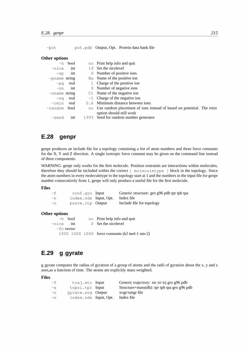
E.28. genpr 215
-pot pot.pdb Output, Opt. Protein data bank file
Other options-h bool no Print help info and quit
-nice int 19 Set the nicelevel-np int 0 Number of positive ions
-pname string Na Name of the positive ion-pq real 1 Charge of the positive ion-nn int 0 Number of negative ions
-nname string Cl Name of the negative ion-nq real -1 Charge of the negative ion
-rmin real 0.6 Minimum distance between ions-random bool no Use random placement of ions instead of based on potential. The rmin
option should still work-seed int 1993 Seed for random number generator
E.28 genpr
genpr produces an include file for a topology containing a list of atom numbers and three force constantsfor the X, Y and Z direction. A single isotropic force constant may be given on the command line insteadof three components.
WARNING: genpr only works for the first molecule. Position restraints are interactions within molecules,therefore they should be included within the correct[ moleculetype ] block in the topology. Sincethe atom numbers in every moleculetype in the topology start at 1 and the numbers in the input file for genprnumber consecutively from 1, genpr will only produce a useful file for the first molecule.
Files-f conf.gro Input Generic structure: gro g96 pdb tpr tpb tpa-n index.ndx Input, Opt. Index file-o posre.itp Output Include file for topology
Other options-h bool no Print help info and quit
-nice int 0 Set the nicelevel-fc vector
1000 1000 1000 force constants (kJ mol-1 nm-2)
E.29 g gyrate
g gyrate computes the radius of gyration of a group of atoms and the radii of gyration about the x, y and zaxes,as a function of time. The atoms are explicitly mass weighted.
Files-f traj.xtc Input Generic trajectory: xtc trr trj gro g96 pdb-s topol.tpr Input Structure+mass(db): tpr tpb tpa gro g96 pdb-o gyrate.xvg Output xvgr/xmgr file-n index.ndx Input, Opt. Index file
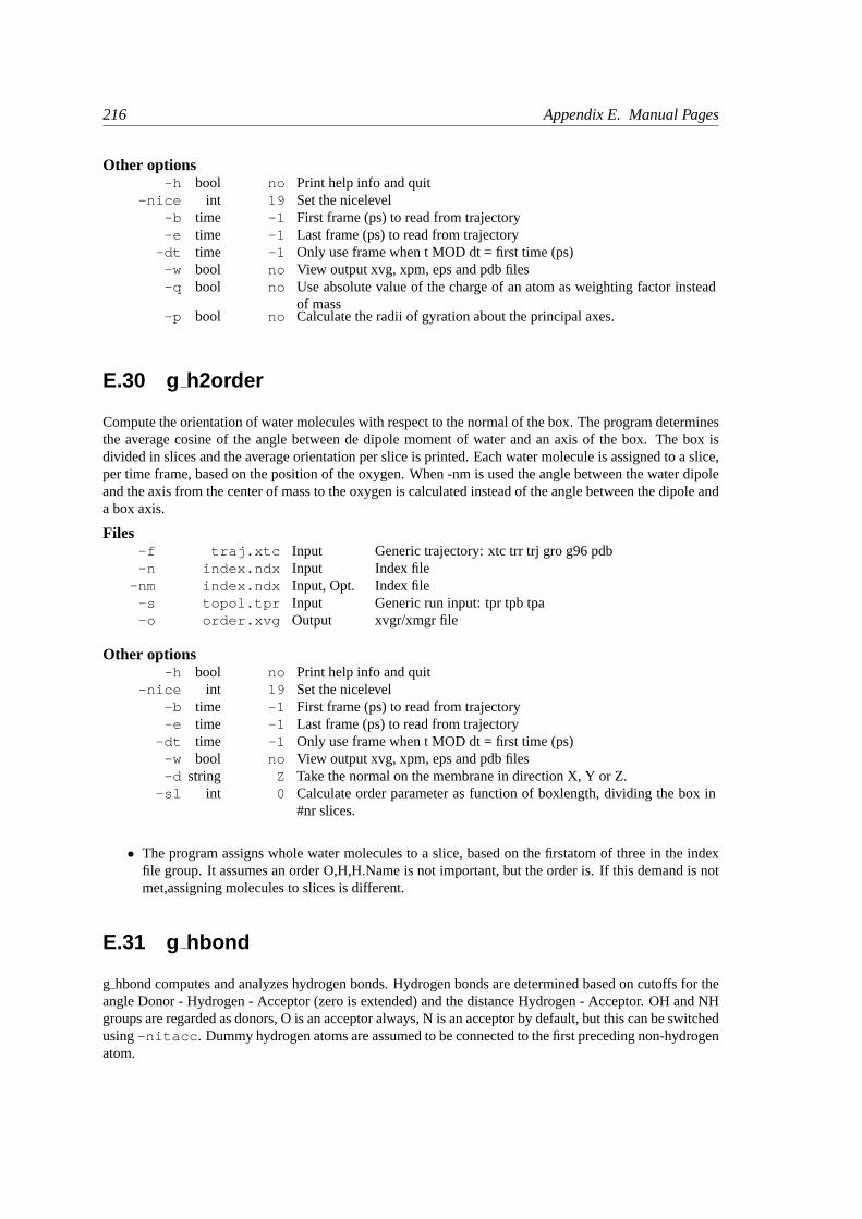
216 Appendix E. Manual Pages
Other options-h bool no Print help info and quit
-nice int 19 Set the nicelevel-b time -1 First frame (ps) to read from trajectory-e time -1 Last frame (ps) to read from trajectory
-dt time -1 Only use frame when t MOD dt = first time (ps)-w bool no View output xvg, xpm, eps and pdb files-q bool no Use absolute value of the charge of an atom as weighting factor instead
of mass-p bool no Calculate the radii of gyration about the principal axes.
E.30 g h2order
Compute the orientation of water molecules with respect to the normal of the box. The program determinesthe average cosine of the angle between de dipole moment of water and an axis of the box. The box isdivided in slices and the average orientation per slice is printed. Each water molecule is assigned to a slice,per time frame, based on the position of the oxygen. When -nm is used the angle between the water dipoleand the axis from the center of mass to the oxygen is calculated instead of the angle between the dipole anda box axis.
Files-f traj.xtc Input Generic trajectory: xtc trr trj gro g96 pdb-n index.ndx Input Index file
-nm index.ndx Input, Opt. Index file-s topol.tpr Input Generic run input: tpr tpb tpa-o order.xvg Output xvgr/xmgr file
Other options-h bool no Print help info and quit
-nice int 19 Set the nicelevel-b time -1 First frame (ps) to read from trajectory-e time -1 Last frame (ps) to read from trajectory
-dt time -1 Only use frame when t MOD dt = first time (ps)-w bool no View output xvg, xpm, eps and pdb files-d string Z Take the normal on the membrane in direction X, Y or Z.
-sl int 0 Calculate order parameter as function of boxlength, dividing the box in#nr slices.
• The program assigns whole water molecules to a slice, based on the firstatom of three in the indexfile group. It assumes an order O,H,H.Name is not important, but the order is. If this demand is notmet,assigning molecules to slices is different.
E.31 g hbond
g hbond computes and analyzes hydrogen bonds. Hydrogen bonds are determined based on cutoffs for theangle Donor - Hydrogen - Acceptor (zero is extended) and the distance Hydrogen - Acceptor. OH and NHgroups are regarded as donors, O is an acceptor always, N is an acceptor by default, but this can be switchedusing-nitacc . Dummy hydrogen atoms are assumed to be connected to the first preceding non-hydrogenatom.

E.31. ghbond 217
You need to specify two groups for analysis, which must be either identical or non-overlapping. All hydro-gen bonds between the two groups are analyzed.
If you set -shell, you will be asked for an additional index group which should contain exactly one atom. Inthis case, only hydrogen bonds between atoms within the shell distance from the one atom are considered.
It is also possible to analyse specific hydrogen bonds with-sel . This index file must contain a group ofatom triplets Donor Hydrogen Acceptor, in the following way:
[ selected ]20 21 2425 26 291 3 6
Note that the triplets need not be on separate lines. Each atom triplet specifies a hydrogen bond to beanalyzed, note also that no check is made for the types of atoms.
-ins turns on computing solvent insertion into hydrogen bonds. In this case an additional group must beselected, specifying the solvent molecules.
Output:-num : number of hydrogen bonds as a function of time.-ac : average over all autocorrelations of the existence functions (either 0 or 1) of all hydrogen bonds.-dist : distance distribution of all hydrogen bonds.-ang : angle distribution of all hydrogen bonds.-hx : the number of n-n+i hydrogen bonds as a function of time where n and n+i stand for residue numbersand i ranges from 0 to 6. This includes the n-n+3, n-n+4 and n-n+5 hydrogen bonds associated with helicesin proteins.-hbn : all selected groups, donors, hydrogens and acceptors for selected groups, all hydrogen bonded atomsfrom all groups and all solvent atoms involved in insertion.-hbm : existence matrix for all hydrogen bonds over all frames, this also contains information on solventinsertion into hydrogen bonds. Ordering is identical to that in-hbn index file.-da : write out the number of donors and acceptors analyzed for each timeframe. This is especially usefullwhen using-shell .
Files-f traj.xtc Input Generic trajectory: xtc trr trj gro g96 pdb-s topol.tpr Input Generic run input: tpr tpb tpa-n index.ndx Input, Opt. Index file-g hbond.log Output, Opt. Log file
-sel select.ndx Input, Opt. Index file-num hbnum.xvg Output xvgr/xmgr file
-ac hbac.xvg Output, Opt. xvgr/xmgr file-dist hbdist.xvg Output, Opt. xvgr/xmgr file
-ang hbang.xvg Output, Opt. xvgr/xmgr file-hx hbhelix.xvg Output, Opt. xvgr/xmgr file
-hbn hbond.ndx Output, Opt. Index file-hbm hbmap.xpm Output, Opt. X PixMap compatible matrix file
-da danum.xvg Output, Opt. xvgr/xmgr file
Other options-h bool no Print help info and quit
-nice int 19 Set the nicelevel-b time -1 First frame (ps) to read from trajectory-e time -1 Last frame (ps) to read from trajectory
-dt time -1 Only use frame when t MOD dt = first time (ps)
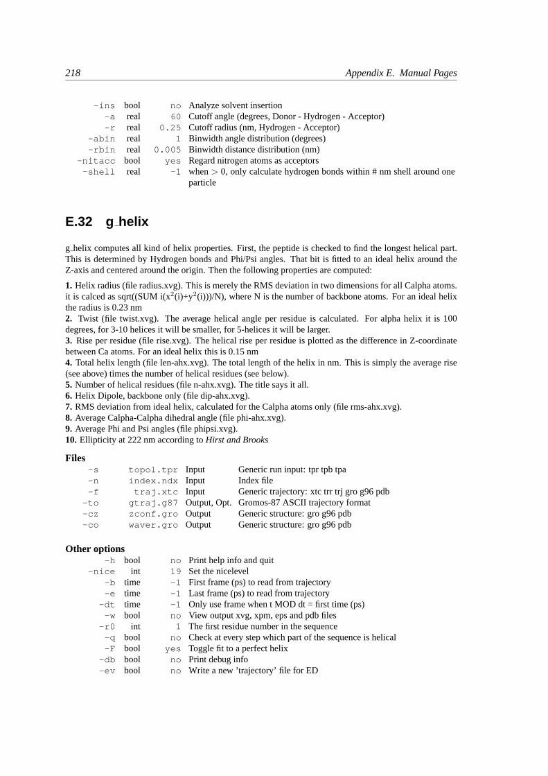
218 Appendix E. Manual Pages
-ins bool no Analyze solvent insertion-a real 60 Cutoff angle (degrees, Donor - Hydrogen - Acceptor)-r real 0.25 Cutoff radius (nm, Hydrogen - Acceptor)
-abin real 1 Binwidth angle distribution (degrees)-rbin real 0.005 Binwidth distance distribution (nm)
-nitacc bool yes Regard nitrogen atoms as acceptors-shell real -1 when> 0, only calculate hydrogen bonds within # nm shell around one
particle
E.32 g helix
g helix computes all kind of helix properties. First, the peptide is checked to find the longest helical part.This is determined by Hydrogen bonds and Phi/Psi angles. That bit is fitted to an ideal helix around theZ-axis and centered around the origin. Then the following properties are computed:
1. Helix radius (file radius.xvg). This is merely the RMS deviation in two dimensions for all Calpha atoms.it is calced as sqrt((SUM i(x2(i)+y2(i)))/N), where N is the number of backbone atoms. For an ideal helixthe radius is 0.23 nm2. Twist (file twist.xvg). The average helical angle per residue is calculated. For alpha helix it is 100degrees, for 3-10 helices it will be smaller, for 5-helices it will be larger.3. Rise per residue (file rise.xvg). The helical rise per residue is plotted as the difference in Z-coordinatebetween Ca atoms. For an ideal helix this is 0.15 nm4. Total helix length (file len-ahx.xvg). The total length of the helix in nm. This is simply the average rise(see above) times the number of helical residues (see below).5. Number of helical residues (file n-ahx.xvg). The title says it all.6. Helix Dipole, backbone only (file dip-ahx.xvg).7. RMS deviation from ideal helix, calculated for the Calpha atoms only (file rms-ahx.xvg).8. Average Calpha-Calpha dihedral angle (file phi-ahx.xvg).9. Average Phi and Psi angles (file phipsi.xvg).10. Ellipticity at 222 nm according toHirst and Brooks
Files-s topol.tpr Input Generic run input: tpr tpb tpa-n index.ndx Input Index file-f traj.xtc Input Generic trajectory: xtc trr trj gro g96 pdb
-to gtraj.g87 Output, Opt. Gromos-87 ASCII trajectory format-cz zconf.gro Output Generic structure: gro g96 pdb-co waver.gro Output Generic structure: gro g96 pdb
Other options-h bool no Print help info and quit
-nice int 19 Set the nicelevel-b time -1 First frame (ps) to read from trajectory-e time -1 Last frame (ps) to read from trajectory
-dt time -1 Only use frame when t MOD dt = first time (ps)-w bool no View output xvg, xpm, eps and pdb files
-r0 int 1 The first residue number in the sequence-q bool no Check at every step which part of the sequence is helical-F bool yes Toggle fit to a perfect helix
-db bool no Print debug info-ev bool no Write a new ’trajectory’ file for ED
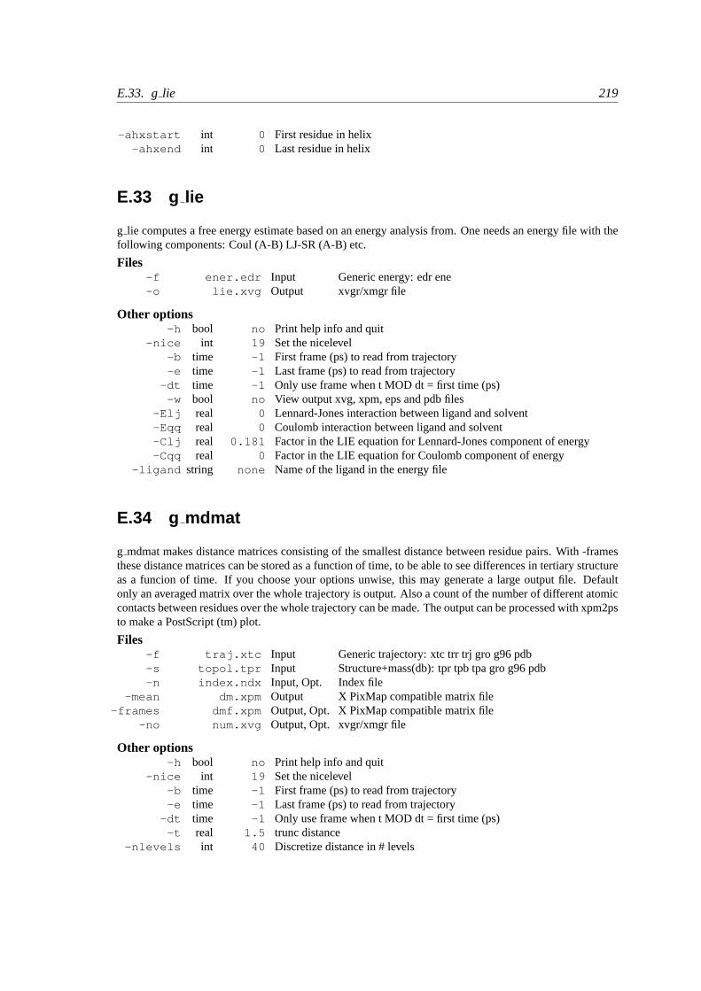
E.33. glie 219
-ahxstart int 0 First residue in helix-ahxend int 0 Last residue in helix
E.33 g lie
g lie computes a free energy estimate based on an energy analysis from. One needs an energy file with thefollowing components: Coul (A-B) LJ-SR (A-B) etc.
Files-f ener.edr Input Generic energy: edr ene-o lie.xvg Output xvgr/xmgr file
Other options-h bool no Print help info and quit
-nice int 19 Set the nicelevel-b time -1 First frame (ps) to read from trajectory-e time -1 Last frame (ps) to read from trajectory
-dt time -1 Only use frame when t MOD dt = first time (ps)-w bool no View output xvg, xpm, eps and pdb files
-Elj real 0 Lennard-Jones interaction between ligand and solvent-Eqq real 0 Coulomb interaction between ligand and solvent-Clj real 0.181 Factor in the LIE equation for Lennard-Jones component of energy-Cqq real 0 Factor in the LIE equation for Coulomb component of energy
-ligand string none Name of the ligand in the energy file
E.34 g mdmat
g mdmat makes distance matrices consisting of the smallest distance between residue pairs. With -framesthese distance matrices can be stored as a function of time, to be able to see differences in tertiary structureas a funcion of time. If you choose your options unwise, this may generate a large output file. Defaultonly an averaged matrix over the whole trajectory is output. Also a count of the number of different atomiccontacts between residues over the whole trajectory can be made. The output can be processed with xpm2psto make a PostScript (tm) plot.
Files-f traj.xtc Input Generic trajectory: xtc trr trj gro g96 pdb-s topol.tpr Input Structure+mass(db): tpr tpb tpa gro g96 pdb-n index.ndx Input, Opt. Index file
-mean dm.xpm Output X PixMap compatible matrix file-frames dmf.xpm Output, Opt. X PixMap compatible matrix file
-no num.xvg Output, Opt. xvgr/xmgr file
Other options-h bool no Print help info and quit
-nice int 19 Set the nicelevel-b time -1 First frame (ps) to read from trajectory-e time -1 Last frame (ps) to read from trajectory
-dt time -1 Only use frame when t MOD dt = first time (ps)-t real 1.5 trunc distance
-nlevels int 40 Discretize distance in # levels
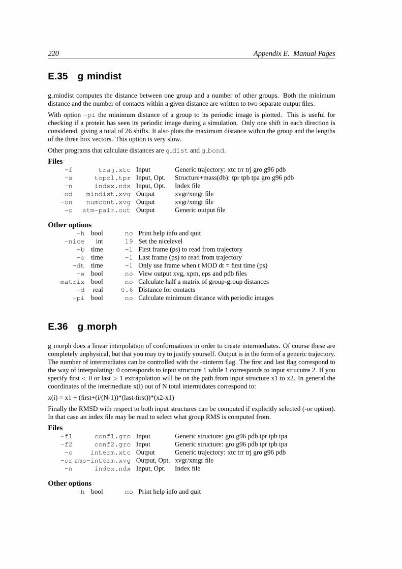
220 Appendix E. Manual Pages
E.35 g mindist
g mindist computes the distance between one group and a number of other groups. Both the minimumdistance and the number of contacts within a given distance are written to two separate output files.
With option -pi the minimum distance of a group to its periodic image is plotted. This is useful forchecking if a protein has seen its periodic image during a simulation. Only one shift in each direction isconsidered, giving a total of 26 shifts. It also plots the maximum distance within the group and the lengthsof the three box vectors. This option is very slow.
Other programs that calculate distances areg dist andg bond .
Files-f traj.xtc Input Generic trajectory: xtc trr trj gro g96 pdb-s topol.tpr Input, Opt. Structure+mass(db): tpr tpb tpa gro g96 pdb-n index.ndx Input, Opt. Index file
-od mindist.xvg Output xvgr/xmgr file-on numcont.xvg Output xvgr/xmgr file
-o atm-pair.out Output Generic output file
Other options-h bool no Print help info and quit
-nice int 19 Set the nicelevel-b time -1 First frame (ps) to read from trajectory-e time -1 Last frame (ps) to read from trajectory
-dt time -1 Only use frame when t MOD dt = first time (ps)-w bool no View output xvg, xpm, eps and pdb files
-matrix bool no Calculate half a matrix of group-group distances-d real 0.6 Distance for contacts
-pi bool no Calculate minimum distance with periodic images
E.36 g morph
g morph does a linear interpolation of conformations in order to create intermediates. Of course these arecompletely unphysical, but that you may try to justify yourself. Output is in the form of a generic trajectory.The number of intermediates can be controlled with the -ninterm flag. The first and last flag correspond tothe way of interpolating: 0 corresponds to input structure 1 while 1 corresponds to input strucutre 2. If youspecify first< 0 or last> 1 extrapolation will be on the path from input structure x1 to x2. In general thecoordinates of the intermediate x(i) out of N total intermidates correspond to:
x(i) = x1 + (first+(i/(N-1))*(last-first))*(x2-x1)
Finally the RMSD with respect to both input structures can be computed if explicitly selected (-or option).In that case an index file may be read to select what group RMS is computed from.
Files-f1 conf1.gro Input Generic structure: gro g96 pdb tpr tpb tpa-f2 conf2.gro Input Generic structure: gro g96 pdb tpr tpb tpa
-o interm.xtc Output Generic trajectory: xtc trr trj gro g96 pdb-or rms-interm.xvg Output, Opt. xvgr/xmgr file
-n index.ndx Input, Opt. Index file
Other options-h bool no Print help info and quit
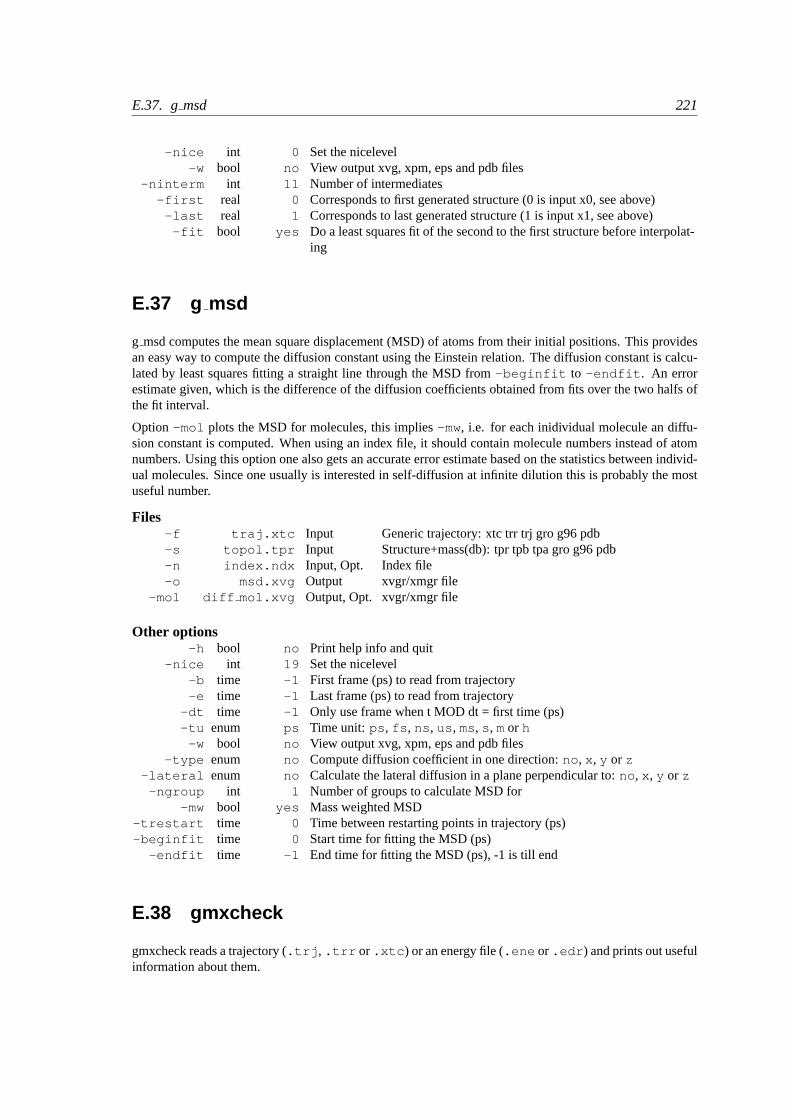
E.37. gmsd 221
-nice int 0 Set the nicelevel-w bool no View output xvg, xpm, eps and pdb files
-ninterm int 11 Number of intermediates-first real 0 Corresponds to first generated structure (0 is input x0, see above)
-last real 1 Corresponds to last generated structure (1 is input x1, see above)-fit bool yes Do a least squares fit of the second to the first structure before interpolat-
ing
E.37 g msd
g msd computes the mean square displacement (MSD) of atoms from their initial positions. This providesan easy way to compute the diffusion constant using the Einstein relation. The diffusion constant is calcu-lated by least squares fitting a straight line through the MSD from-beginfit to -endfit . An errorestimate given, which is the difference of the diffusion coefficients obtained from fits over the two halfs ofthe fit interval.
Option -mol plots the MSD for molecules, this implies-mw, i.e. for each inidividual molecule an diffu-sion constant is computed. When using an index file, it should contain molecule numbers instead of atomnumbers. Using this option one also gets an accurate error estimate based on the statistics between individ-ual molecules. Since one usually is interested in self-diffusion at infinite dilution this is probably the mostuseful number.
Files-f traj.xtc Input Generic trajectory: xtc trr trj gro g96 pdb-s topol.tpr Input Structure+mass(db): tpr tpb tpa gro g96 pdb-n index.ndx Input, Opt. Index file-o msd.xvg Output xvgr/xmgr file
-mol diff mol.xvg Output, Opt. xvgr/xmgr file
Other options-h bool no Print help info and quit
-nice int 19 Set the nicelevel-b time -1 First frame (ps) to read from trajectory-e time -1 Last frame (ps) to read from trajectory
-dt time -1 Only use frame when t MOD dt = first time (ps)-tu enum ps Time unit: ps , fs , ns , us , ms, s , mor h
-w bool no View output xvg, xpm, eps and pdb files-type enum no Compute diffusion coefficient in one direction:no , x , y or z
-lateral enum no Calculate the lateral diffusion in a plane perpendicular to:no , x , y or z-ngroup int 1 Number of groups to calculate MSD for
-mw bool yes Mass weighted MSD-trestart time 0 Time between restarting points in trajectory (ps)-beginfit time 0 Start time for fitting the MSD (ps)
-endfit time -1 End time for fitting the MSD (ps), -1 is till end
E.38 gmxcheck
gmxcheck reads a trajectory (.trj , .trr or .xtc ) or an energy file (.ene or .edr ) and prints out usefulinformation about them.
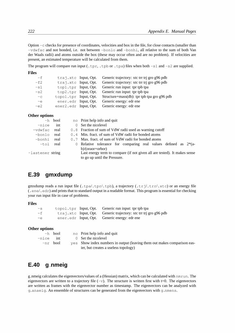
222 Appendix E. Manual Pages
Option-c checks for presence of coordinates, velocities and box in the file, for close contacts (smaller than-vdwfac and not bonded, i.e. not between-bonlo and -bonhi , all relative to the sum of both Vander Waals radii) and atoms outside the box (these may occur often and are no problem). If velocities arepresent, an estimated temperature will be calculated from them.
The program will compare run input (.tpr , .tpb or .tpa ) files when both-s1 and-s2 are supplied.
Files-f traj.xtc Input, Opt. Generic trajectory: xtc trr trj gro g96 pdb
-f2 traj.xtc Input, Opt. Generic trajectory: xtc trr trj gro g96 pdb-s1 top1.tpr Input, Opt. Generic run input: tpr tpb tpa-s2 top2.tpr Input, Opt. Generic run input: tpr tpb tpa
-c topol.tpr Input, Opt. Structure+mass(db): tpr tpb tpa gro g96 pdb-e ener.edr Input, Opt. Generic energy: edr ene
-e2 ener2.edr Input, Opt. Generic energy: edr ene
Other options-h bool no Print help info and quit
-nice int 0 Set the nicelevel-vdwfac real 0.8 Fraction of sum of VdW radii used as warning cutoff
-bonlo real 0.4 Min. fract. of sum of VdW radii for bonded atoms-bonhi real 0.7 Max. fract. of sum of VdW radii for bonded atoms
-tol real 0 Relative tolerance for comparing real values defined as 2*(a-b)/(oraor+orbor)
-lastener string Last energy term to compare (if not given all are tested). It makes senseto go up until the Pressure.
E.39 gmxdump
gmxdump reads a run input file (.tpa /.tpr /.tpb ), a trajectory (.trj /.trr /.xtc ) or an energy file(.ene /.edr ) and prints that to standard output in a readable format. This program is essential for checkingyour run input file in case of problems.
Files-s topol.tpr Input, Opt. Generic run input: tpr tpb tpa-f traj.xtc Input, Opt. Generic trajectory: xtc trr trj gro g96 pdb-e ener.edr Input, Opt. Generic energy: edr ene
Other options-h bool no Print help info and quit
-nice int 0 Set the nicelevel-nr bool yes Show index numbers in output (leaving them out makes comparison eas-
ier, but creates a useless topology)
E.40 g nmeig
g nmeig calculates the eigenvectors/values of a (Hessian) matrix, which can be calculated withnmrun . Theeigenvectors are written to a trajectory file (-v ). The structure is written first with t=0. The eigenvectorsare written as frames with the eigenvector number as timestamp. The eigenvectors can be analyzed withg anaeig . An ensemble of structures can be generated from the eigenvectors withg nmens.
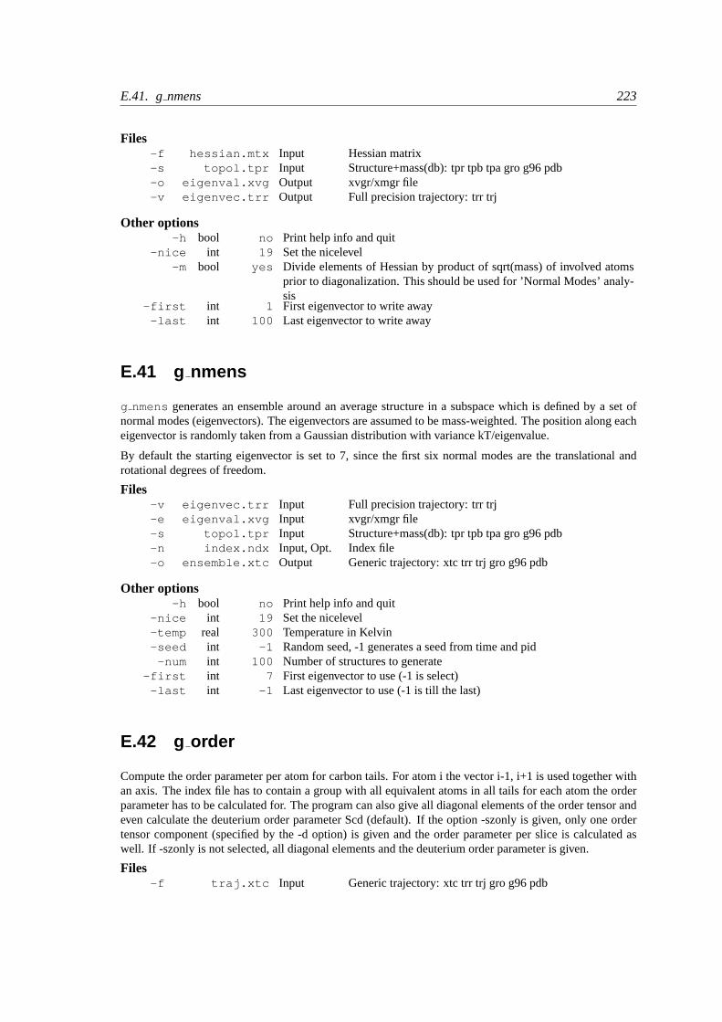
E.41. gnmens 223
Files-f hessian.mtx Input Hessian matrix-s topol.tpr Input Structure+mass(db): tpr tpb tpa gro g96 pdb-o eigenval.xvg Output xvgr/xmgr file-v eigenvec.trr Output Full precision trajectory: trr trj
Other options-h bool no Print help info and quit
-nice int 19 Set the nicelevel-m bool yes Divide elements of Hessian by product of sqrt(mass) of involved atoms
prior to diagonalization. This should be used for ’Normal Modes’ analy-sis
-first int 1 First eigenvector to write away-last int 100 Last eigenvector to write away
E.41 g nmens
g nmens generates an ensemble around an average structure in a subspace which is defined by a set ofnormal modes (eigenvectors). The eigenvectors are assumed to be mass-weighted. The position along eacheigenvector is randomly taken from a Gaussian distribution with variance kT/eigenvalue.
By default the starting eigenvector is set to 7, since the first six normal modes are the translational androtational degrees of freedom.
Files-v eigenvec.trr Input Full precision trajectory: trr trj-e eigenval.xvg Input xvgr/xmgr file-s topol.tpr Input Structure+mass(db): tpr tpb tpa gro g96 pdb-n index.ndx Input, Opt. Index file-o ensemble.xtc Output Generic trajectory: xtc trr trj gro g96 pdb
Other options-h bool no Print help info and quit
-nice int 19 Set the nicelevel-temp real 300 Temperature in Kelvin-seed int -1 Random seed, -1 generates a seed from time and pid
-num int 100 Number of structures to generate-first int 7 First eigenvector to use (-1 is select)
-last int -1 Last eigenvector to use (-1 is till the last)
E.42 g order
Compute the order parameter per atom for carbon tails. For atom i the vector i-1, i+1 is used together withan axis. The index file has to contain a group with all equivalent atoms in all tails for each atom the orderparameter has to be calculated for. The program can also give all diagonal elements of the order tensor andeven calculate the deuterium order parameter Scd (default). If the option -szonly is given, only one ordertensor component (specified by the -d option) is given and the order parameter per slice is calculated aswell. If -szonly is not selected, all diagonal elements and the deuterium order parameter is given.
Files-f traj.xtc Input Generic trajectory: xtc trr trj gro g96 pdb

224 Appendix E. Manual Pages
-n index.ndx Input Index file-s topol.tpr Input Generic run input: tpr tpb tpa-o order.xvg Output xvgr/xmgr file
-od deuter.xvg Output xvgr/xmgr file-os sliced.xvg Output xvgr/xmgr file
Other options-h bool no Print help info and quit
-nice int 19 Set the nicelevel-b time -1 First frame (ps) to read from trajectory-e time -1 Last frame (ps) to read from trajectory
-dt time -1 Only use frame when t MOD dt = first time (ps)-w bool no View output xvg, xpm, eps and pdb files-d enum z Direction of the normal on the membrane:z , x or y
-sl int 1 Calculate order parameter as function of boxlength, dividing the box in#nr slices.
-szonly bool no Only give Sz element of order tensor. (axis can be specified with -d)-unsat bool no Calculate order parameters for unsaturated carbons. Note that this cannot
be mixed with normal order parameters.
E.43 g potential
Compute the electrostatical potential across the box. The potential iscalculated by first summing the chargesper slice and then integratingtwice of this charge distribution. Periodic boundaries are not taken into ac-count. Reference of potential is taken to be the left side ofthe box. It’s also possible to calculate thepotential in sphericalcoordinates as function of r by calculating a charge distribution inspherical slices andtwice integrating them. epsilonr is taken as 1,2 is more appropriate in many cases
Files-f traj.xtc Input Generic trajectory: xtc trr trj gro g96 pdb-n index.ndx Input Index file-s topol.tpr Input Generic run input: tpr tpb tpa-o potential.xvg Output xvgr/xmgr file
-oc charge.xvg Output xvgr/xmgr file-of field.xvg Output xvgr/xmgr file
Other options-h bool no Print help info and quit
-nice int 19 Set the nicelevel-b time -1 First frame (ps) to read from trajectory-e time -1 Last frame (ps) to read from trajectory
-dt time -1 Only use frame when t MOD dt = first time (ps)-w bool no View output xvg, xpm, eps and pdb files-d string Z Take the normal on the membrane in direction X, Y or Z.
-sl int 10 Calculate potential as function of boxlength, dividing the box in #nrslices.
-cb int 0 Discard first #nr slices of box for integration-ce int 0 Discard last #nr slices of box for integration-tz real 0 Translate all coordinates<distance> in the direction of the box
-spherical bool no Calculate spherical thingie
• Discarding slices for integration should not be necessary.

E.44. grama 225
E.44 g rama
g rama selects the Phi/Psi dihedral combinations from your topology file and computes these as a functionof time. Using simple Unix tools such asgrepyou can select out specific residues.
Files-f traj.xtc Input Generic trajectory: xtc trr trj gro g96 pdb-s topol.tpr Input Generic run input: tpr tpb tpa-o rama.xvg Output xvgr/xmgr file
Other options-h bool no Print help info and quit
-nice int 19 Set the nicelevel-b time -1 First frame (ps) to read from trajectory-e time -1 Last frame (ps) to read from trajectory
-dt time -1 Only use frame when t MOD dt = first time (ps)-w bool no View output xvg, xpm, eps and pdb files
E.45 g rdf
The structure of liquids can be studied by either neutron or X-ray scattering. The most common way todescribe liquid structure is by a radial distribution function. However, this is not easy to obtain from ascattering experiment.
g rdf calculates radial distribution functions in different ways. The normal method is around a (set of)particle(s), the other method is around the center of mass of a set of particles.
If a run input file is supplied (-s ), exclusions defined in that file are taken into account when calculatingthe rdf. The option-cut is meant as an alternative way to avoid intramolecular peaks in the rdf plot. It ishowever better to supply a run input file with a higher number of exclusions. For eg. benzene a topologywith nrexcl set to 5 would eliminate all intramolecular contributions to the rdf. Note that all atoms in theselected groups are used, also the ones that don’t have Lennard-Jones interactions.
Option-cn produces the cumulative number rdf.
To bridge the gap between theory and experiment structure factors can be computed (option-sq ). Thealgorithm uses FFT, the gridspacing of which is determined by option-grid .
Files-f traj.xtc Input Generic trajectory: xtc trr trj gro g96 pdb-s topol.tpr Input, Opt. Structure+mass(db): tpr tpb tpa gro g96 pdb-n index.ndx Input, Opt. Index file-o rdf.xvg Output, Opt. xvgr/xmgr file
-sq sq.xvg Output, Opt. xvgr/xmgr file-cn rdf cn.xvg Output, Opt. xvgr/xmgr file-hq hq.xvg Output, Opt. xvgr/xmgr file
-image sq.xpm Output, Opt. X PixMap compatible matrix file
Other options-h bool no Print help info and quit
-nice int 19 Set the nicelevel-b time -1 First frame (ps) to read from trajectory-e time -1 Last frame (ps) to read from trajectory
-dt time -1 Only use frame when t MOD dt = first time (ps)
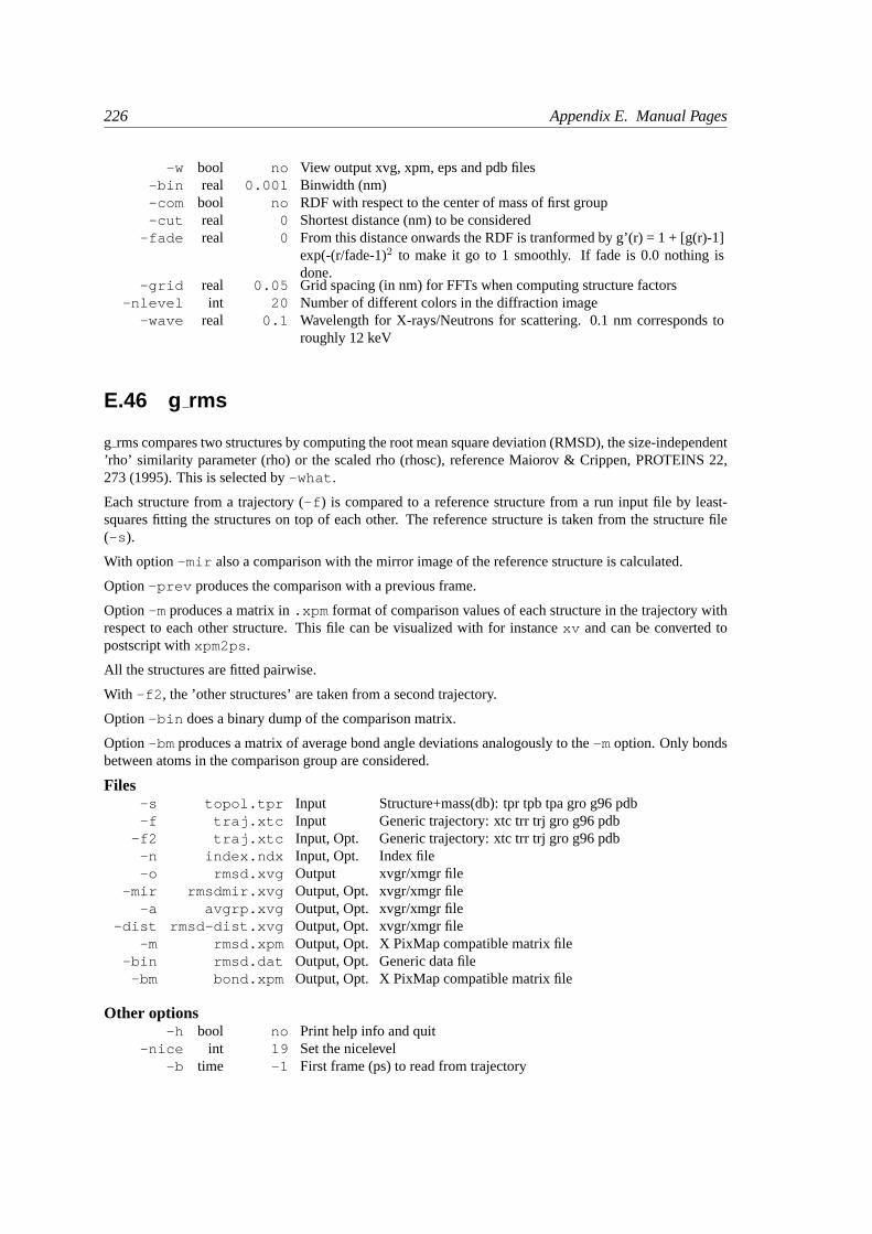
226 Appendix E. Manual Pages
-w bool no View output xvg, xpm, eps and pdb files-bin real 0.001 Binwidth (nm)-com bool no RDF with respect to the center of mass of first group-cut real 0 Shortest distance (nm) to be considered
-fade real 0 From this distance onwards the RDF is tranformed by g’(r) = 1 + [g(r)-1]exp(-(r/fade-1)2 to make it go to 1 smoothly. If fade is 0.0 nothing isdone.
-grid real 0.05 Grid spacing (in nm) for FFTs when computing structure factors-nlevel int 20 Number of different colors in the diffraction image
-wave real 0.1 Wavelength for X-rays/Neutrons for scattering. 0.1 nm corresponds toroughly 12 keV
E.46 g rms
g rms compares two structures by computing the root mean square deviation (RMSD), the size-independent’rho’ similarity parameter (rho) or the scaled rho (rhosc), reference Maiorov & Crippen, PROTEINS 22,273 (1995). This is selected by-what .
Each structure from a trajectory (-f ) is compared to a reference structure from a run input file by least-squares fitting the structures on top of each other. The reference structure is taken from the structure file(-s ).
With option-mir also a comparison with the mirror image of the reference structure is calculated.
Option-prev produces the comparison with a previous frame.
Option-m produces a matrix in.xpm format of comparison values of each structure in the trajectory withrespect to each other structure. This file can be visualized with for instancexv and can be converted topostscript withxpm2ps .
All the structures are fitted pairwise.
With -f2 , the ’other structures’ are taken from a second trajectory.
Option-bin does a binary dump of the comparison matrix.
Option-bm produces a matrix of average bond angle deviations analogously to the-m option. Only bondsbetween atoms in the comparison group are considered.
Files-s topol.tpr Input Structure+mass(db): tpr tpb tpa gro g96 pdb-f traj.xtc Input Generic trajectory: xtc trr trj gro g96 pdb
-f2 traj.xtc Input, Opt. Generic trajectory: xtc trr trj gro g96 pdb-n index.ndx Input, Opt. Index file-o rmsd.xvg Output xvgr/xmgr file
-mir rmsdmir.xvg Output, Opt. xvgr/xmgr file-a avgrp.xvg Output, Opt. xvgr/xmgr file
-dist rmsd-dist.xvg Output, Opt. xvgr/xmgr file-m rmsd.xpm Output, Opt. X PixMap compatible matrix file
-bin rmsd.dat Output, Opt. Generic data file-bm bond.xpm Output, Opt. X PixMap compatible matrix file
Other options-h bool no Print help info and quit
-nice int 19 Set the nicelevel-b time -1 First frame (ps) to read from trajectory
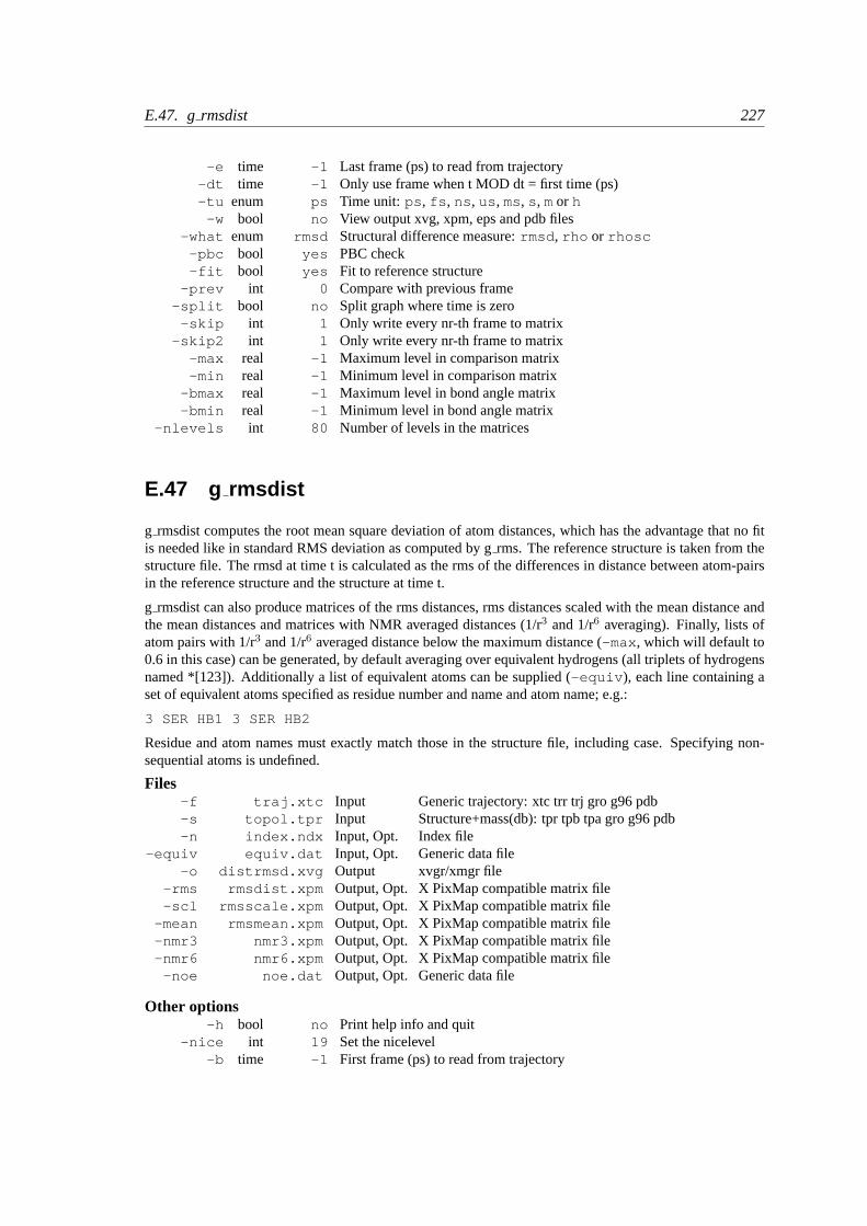
E.47. grmsdist 227
-e time -1 Last frame (ps) to read from trajectory-dt time -1 Only use frame when t MOD dt = first time (ps)-tu enum ps Time unit: ps , fs , ns , us , ms, s , mor h
-w bool no View output xvg, xpm, eps and pdb files-what enum rmsd Structural difference measure:rmsd , rho or rhosc
-pbc bool yes PBC check-fit bool yes Fit to reference structure
-prev int 0 Compare with previous frame-split bool no Split graph where time is zero
-skip int 1 Only write every nr-th frame to matrix-skip2 int 1 Only write every nr-th frame to matrix
-max real -1 Maximum level in comparison matrix-min real -1 Minimum level in comparison matrix
-bmax real -1 Maximum level in bond angle matrix-bmin real -1 Minimum level in bond angle matrix
-nlevels int 80 Number of levels in the matrices
E.47 g rmsdist
g rmsdist computes the root mean square deviation of atom distances, which has the advantage that no fitis needed like in standard RMS deviation as computed by grms. The reference structure is taken from thestructure file. The rmsd at time t is calculated as the rms of the differences in distance between atom-pairsin the reference structure and the structure at time t.
g rmsdist can also produce matrices of the rms distances, rms distances scaled with the mean distance andthe mean distances and matrices with NMR averaged distances (1/r3 and 1/r6 averaging). Finally, lists ofatom pairs with 1/r3 and 1/r6 averaged distance below the maximum distance (-max , which will default to0.6 in this case) can be generated, by default averaging over equivalent hydrogens (all triplets of hydrogensnamed *[123]). Additionally a list of equivalent atoms can be supplied (-equiv ), each line containing aset of equivalent atoms specified as residue number and name and atom name; e.g.:
3 SER HB1 3 SER HB2
Residue and atom names must exactly match those in the structure file, including case. Specifying non-sequential atoms is undefined.
Files-f traj.xtc Input Generic trajectory: xtc trr trj gro g96 pdb-s topol.tpr Input Structure+mass(db): tpr tpb tpa gro g96 pdb-n index.ndx Input, Opt. Index file
-equiv equiv.dat Input, Opt. Generic data file-o distrmsd.xvg Output xvgr/xmgr file
-rms rmsdist.xpm Output, Opt. X PixMap compatible matrix file-scl rmsscale.xpm Output, Opt. X PixMap compatible matrix file
-mean rmsmean.xpm Output, Opt. X PixMap compatible matrix file-nmr3 nmr3.xpm Output, Opt. X PixMap compatible matrix file-nmr6 nmr6.xpm Output, Opt. X PixMap compatible matrix file
-noe noe.dat Output, Opt. Generic data file
Other options-h bool no Print help info and quit
-nice int 19 Set the nicelevel-b time -1 First frame (ps) to read from trajectory
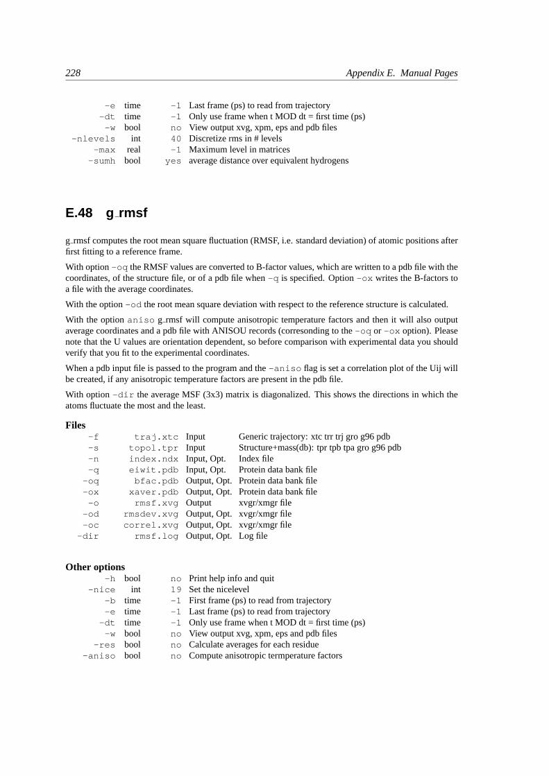
228 Appendix E. Manual Pages
-e time -1 Last frame (ps) to read from trajectory-dt time -1 Only use frame when t MOD dt = first time (ps)
-w bool no View output xvg, xpm, eps and pdb files-nlevels int 40 Discretize rms in # levels
-max real -1 Maximum level in matrices-sumh bool yes average distance over equivalent hydrogens
E.48 g rmsf
g rmsf computes the root mean square fluctuation (RMSF, i.e. standard deviation) of atomic positions afterfirst fitting to a reference frame.
With option-oq the RMSF values are converted to B-factor values, which are written to a pdb file with thecoordinates, of the structure file, or of a pdb file when-q is specified. Option-ox writes the B-factors toa file with the average coordinates.
With the option-od the root mean square deviation with respect to the reference structure is calculated.
With the optionaniso g rmsf will compute anisotropic temperature factors and then it will also outputaverage coordinates and a pdb file with ANISOU records (corresonding to the-oq or -ox option). Pleasenote that the U values are orientation dependent, so before comparison with experimental data you shouldverify that you fit to the experimental coordinates.
When a pdb input file is passed to the program and the-aniso flag is set a correlation plot of the Uij willbe created, if any anisotropic temperature factors are present in the pdb file.
With option -dir the average MSF (3x3) matrix is diagonalized. This shows the directions in which theatoms fluctuate the most and the least.
Files-f traj.xtc Input Generic trajectory: xtc trr trj gro g96 pdb-s topol.tpr Input Structure+mass(db): tpr tpb tpa gro g96 pdb-n index.ndx Input, Opt. Index file-q eiwit.pdb Input, Opt. Protein data bank file
-oq bfac.pdb Output, Opt. Protein data bank file-ox xaver.pdb Output, Opt. Protein data bank file
-o rmsf.xvg Output xvgr/xmgr file-od rmsdev.xvg Output, Opt. xvgr/xmgr file-oc correl.xvg Output, Opt. xvgr/xmgr file
-dir rmsf.log Output, Opt. Log file
Other options-h bool no Print help info and quit
-nice int 19 Set the nicelevel-b time -1 First frame (ps) to read from trajectory-e time -1 Last frame (ps) to read from trajectory
-dt time -1 Only use frame when t MOD dt = first time (ps)-w bool no View output xvg, xpm, eps and pdb files
-res bool no Calculate averages for each residue-aniso bool no Compute anisotropic termperature factors
E.49. grompp 229
E.49 grompp
The gromacs preprocessor reads a molecular topology file, checks the validity of the file, expands thetopology from a molecular description to an atomic description. The topology file contains informationabout molecule types and the number of molecules, the preprocessor copies each molecule as needed.There is no limitation on the number of molecule types. Bonds and bond-angles can be converted intoconstraints, separately for hydrogens and heavy atoms. Then a coordinate file is read and velocities can begenerated from a Maxwellian distribution if requested. grompp also reads parameters for the mdrun (eg.number of MD steps, time step, cut-off), and others such as NEMD parameters, which are corrected so thatthe net acceleration is zero. Eventually a binary file is produced that can serve as the sole input file for theMD program.
grompp uses the atom names from the topology file. The atom names in the coordinate file (option-c )are only read to generate warnings when they do not match the atom names in the topology. Note thatthe atom names are irrelevant for the simulation as only the atom types are used for generating interactionparameters.
grompp calls the c-preprocessor to resolve includes, macros etcetera. To specify a macro-preprocessorother than /lib/cpp (such as m4) you can put a line in your parameter file specifying the path to that cpp.Specifying-pp will get the pre-processed topology file written out.
If your system does not have a c-preprocessor, you can still use grompp, but you do not have access to thefeatures from the cpp. Command line options to the c-preprocessor can be given in the.mdp file. See yourlocal manual (man cpp).
When using position restraints a file with restraint coordinates can be supplied with-r , otherwise con-straining will be done relative to the conformation from the-c option.
Starting coordinates can be read from trajectory with-t . The last frame with coordinates and velocitieswill be read, unless the-time option is used. Note that these velocities will not be used whengen vel= yes in your .mdp file. If you want to continue a crashed run, it is easier to usetpbconv .
When preparing an input file for parallelmdrun it may be advantageous to partition the simulation systemover the nodes in a way in which each node has a similar amount of work. The -shuffle option does justthat. For a single protein in water this does not make a difference, however for a system where you havemany copies of different molecules (e.g. liquid mixture or membrane/water system) the option is definitelya must. The output trajectories will also be shuffled.grompp writes an index file (option-deshuf ) whichcan be used withtrjconv to deshuffle the trajectories.
A further optimization for parallel systems is the-sort option which sorts molecules according to coor-dinates. This must always be used in conjunction with-shuffle , however sorting also works when youhave only one molecule type.
Using the-morse option grompp can convert the harmonic bonds in your topology to morse potentials.This makes it possible to break bonds. For this option to work you need an extra file in your $GMXLIBwith dissociation energy. Use the -debug option to get more information on the workings of this option(look for MORSE in the grompp.log file using less or something like that).
By default all bonded interactions which have constant energy due to dummy atom constructions will beremoved. If this constant energy is not zero, this will result in a shift in the total energy. All bondedinteractions can be kept by turning off-rmdumbds . Additionally, all constraints for distances which willbe constant anyway because of dummy atom constructions will be removed. If any constraints remainwhich involve dummy atoms, a fatal error will result.
To verify your run input file, please make notice of all warnings on the screen, and correct where necessary.Do also look at the contents of themdout.mdp file, this contains comment lines, as well as the input thatgrompp has read. If in doubt you can start grompp with the-debug option which will give you moreinformation in a file called grompp.log (along with real debug info). Finally, you can see the contents of the
230 Appendix E. Manual Pages
run input file with thegmxdumpprogram.
Files-f grompp.mdp Input, Opt. grompp input file with MD parameters
-po mdout.mdp Output grompp input file with MD parameters-c conf.gro Input Generic structure: gro g96 pdb tpr tpb tpa-r conf.gro Input, Opt. Generic structure: gro g96 pdb tpr tpb tpa-n index.ndx Input, Opt. Index file
-deshuf deshuf.ndx Output, Opt. Index file-p topol.top Input Topology file
-pp processed.top Output, Opt. Topology file-o topol.tpr Output Generic run input: tpr tpb tpa-t traj.trr Input, Opt. Full precision trajectory: trr trj
Other options-h bool no Print help info and quit
-nice int 0 Set the nicelevel-v bool yes Be loud and noisy
-time real -1 Take frame at or first after this time.-np int 1 Generate statusfile for # nodes
-shuffle bool no Shuffle molecules over nodes-sort bool no Sort molecules according to X coordinate
-rmdumbds bool yes Remove constant bonded interactions with dummies-load string Releative load capacity of each node on a parallel machine. Be sure to
use quotes around the string, which should contain a number for eachnode
-maxwarn int 10 Number of warnings after which input processing stops-check14 bool no Remove 1-4 interactions without Van der Waals
E.50 g rotacf
g rotacf calculates the rotational correlation function for molecules. Three atoms (i,j,k) must be given inthe index file, defining two vectors ij and jk. The rotational acf is calculated as the autocorrelation functionof the vector n = ij x jk, i.e. the cross product of the two vectors. Since three atoms span a plane, the orderof the three atoms does not matter. Optionally, controlled by the -d switch, you can calculate the rotationalcorrelation function for linear molecules by specifying two atoms (i,j) in the index file.
EXAMPLES
g rotacf -P 1 -nparm 2 -fft -n index -o rotacf-x-P1 -fa expfit-x-P1 -beginfit 2.5 -endfit 20.0
This will calculate the rotational correlation function using a first order Legendre polynomial of the angleof a vector defined by the index file. The correlation function will be fitted from 2.5 ps till 20.0 ps to a twoparameter exponential
Files-f traj.xtc Input Generic trajectory: xtc trr trj gro g96 pdb-s topol.tpr Input Generic run input: tpr tpb tpa-n index.ndx Input Index file-o rotacf.xvg Output xvgr/xmgr file
Other options-h bool no Print help info and quit
E.51. gsaltbr 231
-nice int 19 Set the nicelevel-b time -1 First frame (ps) to read from trajectory-e time -1 Last frame (ps) to read from trajectory
-dt time -1 Only use frame when t MOD dt = first time (ps)-w bool no View output xvg, xpm, eps and pdb files-d bool no Use index doublets (vectors) for correlation function instead of triplets
(planes)-aver bool yes Average over molecules
-acflen int -1 Length of the ACF, default is half the number of frames-normalize bool yes Normalize ACF
-P enum 0 Order of Legendre polynomial for ACF (0 indicates none):0, 1, 2 or 3-fitfn enum none Fit function: none , exp , aexp , exp exp , vac , exp5 or exp7
-ncskip int 0 Skip N points in the output file of correlation functions-beginfit real 0 Time where to begin the exponential fit of the correlation function
-endfit real -1 Time where to end the exponential fit of the correlation function, -1 is tillthe end
E.51 g saltbr
g saltbr plots the difference between all combination of charged groups as a function of time. The groupsare combined in different ways.A minimum distance can be given, (eg. the cut-off), then groups that arenever closer than that distance will not be plotted.Output will be in a number of fixed filenames, min-min.xvg,min-plus.xvg and plus-plus.xvg, or files forevery individual ion-pair if selected
Files-f traj.xtc Input Generic trajectory: xtc trr trj gro g96 pdb-s topol.tpr Input Generic run input: tpr tpb tpa
Other options-h bool no Print help info and quit
-nice int 19 Set the nicelevel-b time -1 First frame (ps) to read from trajectory-e time -1 Last frame (ps) to read from trajectory
-dt time -1 Only use frame when t MOD dt = first time (ps)-t real 1000 trunc distance
-sep bool no Use separate files for each interaction (may be MANY)
E.52 g sas
g sas computes hydrophobic, hydrophilic and total solvent accessible surface area. As a side effect theConnolly surface can be generated as well in a pdb file where the nodes are represented as atoms and thevertices connecting the nearest nodes as CONECT records. The area can be plotted per atom and per residueas well (option -ao). In combination with the latter option anitp file can be generated (option -i) whichcan be used to restrain surface atoms.
By default, periodic boundary conditions are taken into account, this can be turned off using the -pbc option.
Files-f traj.xtc Input Generic trajectory: xtc trr trj gro g96 pdb
232 Appendix E. Manual Pages
-s topol.tpr Input Generic run input: tpr tpb tpa-o area.xvg Output xvgr/xmgr file-r resarea.xvg Output xvgr/xmgr file-q connelly.pdb Output, Opt. Protein data bank file
-ao atomarea.xvg Output, Opt. xvgr/xmgr file-n index.ndx Input, Opt. Index file-i surfat.itp Output, Opt. Include file for topology
Other options-h bool no Print help info and quit
-nice int 19 Set the nicelevel-b time -1 First frame (ps) to read from trajectory-e time -1 Last frame (ps) to read from trajectory
-dt time -1 Only use frame when t MOD dt = first time (ps)-w bool no View output xvg, xpm, eps and pdb files
-solsize real 0.14 Radius of the solvent probe (nm)-ndots int 24 Number of dots per sphere, more dots means more accuracy
-qmax real 0.2 The maximum charge (e, absolute value) of a hydrophobic atom-minarea real 0.5 The minimum area (nm2) to count an atom as a surface atom when writ-
ing a position restraint file (see help)-skip int 1 Do only every nth frame
-pbc bool yes Take periodicity into account-prot bool yes Output the protein to the connelly pdb file too
-dgs real 0 default value for solvation free energy per area (kJ/mol/nm2)
E.53 g sgangle
Compute the angle and distance between two groups. The groups are defined by a number of atoms givenin an index file and may be two or three atoms in size. The angles calculated depend on the order in whichthe atoms are given. Giving for instance 5 6 will rotate the vector 5-6 with 180 degrees compared to giving6 5.
If three atoms are given, the normal on the plane spanned by those three atoms will be calculated, using theformula P1P2 x P1P3. The cos of the angle is calculated, using the inproduct of the two normalized vectors.
Here is what some of the file options do:-oa: Angle between the two groups specified in the index file. If a group contains three atoms the normalto the plane defined by those three atoms will be used. If a group contains two atoms, the vector defined bythose two atoms will be used.-od: Distance between two groups. Distance is taken from the center of one group to the center of the othergroup.-od1: If one plane and one vector is given, the distances for each of the atoms from the center of the planeis given seperately.-od2: For two planes this option has no meaning.
Files-f traj.xtc Input Generic trajectory: xtc trr trj gro g96 pdb-n index.ndx Input Index file-s topol.tpr Input Generic run input: tpr tpb tpa
-oa sg angle.xvg Output xvgr/xmgr file-od sg dist.xvg Output xvgr/xmgr file
-od1 sg dist1.xvg Output xvgr/xmgr file-od2 sg dist2.xvg Output xvgr/xmgr file
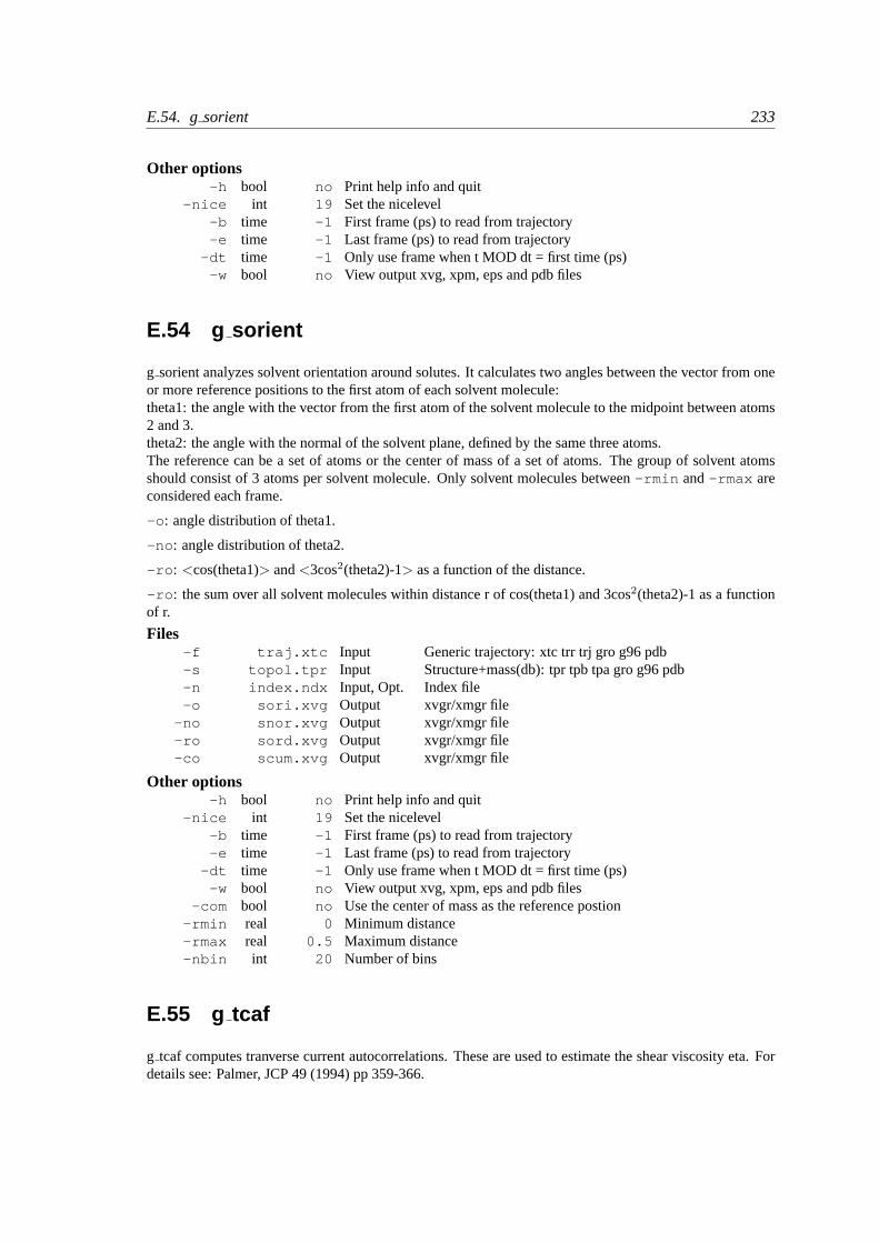
E.54. gsorient 233
Other options-h bool no Print help info and quit
-nice int 19 Set the nicelevel-b time -1 First frame (ps) to read from trajectory-e time -1 Last frame (ps) to read from trajectory
-dt time -1 Only use frame when t MOD dt = first time (ps)-w bool no View output xvg, xpm, eps and pdb files
E.54 g sorient
g sorient analyzes solvent orientation around solutes. It calculates two angles between the vector from oneor more reference positions to the first atom of each solvent molecule:theta1: the angle with the vector from the first atom of the solvent molecule to the midpoint between atoms2 and 3.theta2: the angle with the normal of the solvent plane, defined by the same three atoms.The reference can be a set of atoms or the center of mass of a set of atoms. The group of solvent atomsshould consist of 3 atoms per solvent molecule. Only solvent molecules between-rmin and-rmax areconsidered each frame.
-o : angle distribution of theta1.
-no : angle distribution of theta2.
-ro : <cos(theta1)> and<3cos2(theta2)-1> as a function of the distance.
-ro : the sum over all solvent molecules within distance r of cos(theta1) and 3cos2(theta2)-1 as a functionof r.
Files-f traj.xtc Input Generic trajectory: xtc trr trj gro g96 pdb-s topol.tpr Input Structure+mass(db): tpr tpb tpa gro g96 pdb-n index.ndx Input, Opt. Index file-o sori.xvg Output xvgr/xmgr file
-no snor.xvg Output xvgr/xmgr file-ro sord.xvg Output xvgr/xmgr file-co scum.xvg Output xvgr/xmgr file
Other options-h bool no Print help info and quit
-nice int 19 Set the nicelevel-b time -1 First frame (ps) to read from trajectory-e time -1 Last frame (ps) to read from trajectory
-dt time -1 Only use frame when t MOD dt = first time (ps)-w bool no View output xvg, xpm, eps and pdb files
-com bool no Use the center of mass as the reference postion-rmin real 0 Minimum distance-rmax real 0.5 Maximum distance-nbin int 20 Number of bins
E.55 g tcaf
g tcaf computes tranverse current autocorrelations. These are used to estimate the shear viscosity eta. Fordetails see: Palmer, JCP 49 (1994) pp 359-366.
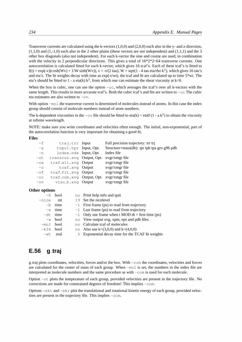
234 Appendix E. Manual Pages
Transverse currents are calculated using the k-vectors (1,0,0) and (2,0,0) each also in the y- and z-direction,(1,1,0) and (1,-1,0) each also in the 2 other plains (these vectors are not independent) and (1,1,1) and the 3other box diagonals (also not independent). For each k-vector the sine and cosine are used, in combinationwith the velocity in 2 perpendicular directions. This gives a total of 16*2*2=64 transverse currents. Oneautocorrelation is calculated fitted for each k-vector, which gives 16 tcaf’s. Each of these tcaf’s is fitted tof(t) = exp(-v)(cosh(Wv) + 1/W sinh(Wv)), v = -t/(2 tau), W = sqrt(1 - 4 tau eta/rho k2), which gives 16 tau’sand eta’s. The fit weights decay with time as exp(-t/wt), the tcaf and fit are calculated up to time 5*wt. Theeta’s should be fitted to 1 - a eta(k) k2, from which one can estimate the shear viscosity at k=0.
When the box is cubic, one can use the option-oc , which averages the tcaf’s over all k-vectors with thesame length. This results in more accurate tcaf’s. Both the cubic tcaf’s and fits are written to-oc The cubiceta estimates are also written to-ov .
With option-mol the transverse current is determined of molecules instead of atoms. In this case the indexgroup should consist of molecule numbers instead of atom numbers.
The k-dependent viscosities in the-ov file should be fitted to eta(k) = eta0 (1 - a k2) to obtain the viscosityat infinite wavelength.
NOTE: make sure you write coordinates and velocities often enough. The initial, non-exponential, part ofthe autocorrelation function is very important for obtaining a good fit.
Files-f traj.trr Input Full precision trajectory: trr trj-s topol.tpr Input, Opt. Structure+mass(db): tpr tpb tpa gro g96 pdb-n index.ndx Input, Opt. Index file
-ot transcur.xvg Output, Opt. xvgr/xmgr file-oa tcaf all.xvg Output xvgr/xmgr file
-o tcaf.xvg Output xvgr/xmgr file-of tcaf fit.xvg Output xvgr/xmgr file-oc tcaf cub.xvg Output, Opt. xvgr/xmgr file-ov visc k.xvg Output xvgr/xmgr file
Other options-h bool no Print help info and quit
-nice int 19 Set the nicelevel-b time -1 First frame (ps) to read from trajectory-e time -1 Last frame (ps) to read from trajectory
-dt time -1 Only use frame when t MOD dt = first time (ps)-w bool no View output xvg, xpm, eps and pdb files
-mol bool no Calculate tcaf of molecules-k34 bool no Also use k=(3,0,0) and k=(4,0,0)
-wt real 5 Exponential decay time for the TCAF fit weights
E.56 g traj
g traj plots coordinates, velocities, forces and/or the box. With-com the coordinates, velocities and forcesare calculated for the center of mass of each group. When-mol is set, the numbers in the index file areinterpreted as molecule numbers and the same procedure as with-com is used for each molecule.
Option -ot plots the temperature of each group, provided velocities are present in the trajectory file. Nocorrections are made for constrained degrees of freedom! This implies-com .
Options-ekt and-ekr plot the translational and rotational kinetic energy of each group, provided veloc-ities are present in the trajectory file. This implies-com .
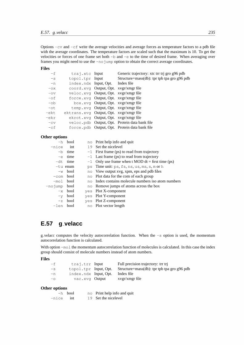
E.57. gvelacc 235
Options-cv and-cf write the average velocities and average forces as temperature factors to a pdb filewith the average coordinates. The temperature factors are scaled such that the maximum is 10. To get thevelocities or forces of one frame set both-b and-e to the time of desired frame. When averaging overframes you might need to use the-nojump option to obtain the correct average coordinates.
Files-f traj.xtc Input Generic trajectory: xtc trr trj gro g96 pdb-s topol.tpr Input Structure+mass(db): tpr tpb tpa gro g96 pdb-n index.ndx Input, Opt. Index file
-ox coord.xvg Output, Opt. xvgr/xmgr file-ov veloc.xvg Output, Opt. xvgr/xmgr file-of force.xvg Output, Opt. xvgr/xmgr file-ob box.xvg Output, Opt. xvgr/xmgr file-ot temp.xvg Output, Opt. xvgr/xmgr file
-ekt ektrans.xvg Output, Opt. xvgr/xmgr file-ekr ekrot.xvg Output, Opt. xvgr/xmgr file
-cv veloc.pdb Output, Opt. Protein data bank file-cf force.pdb Output, Opt. Protein data bank file
Other options-h bool no Print help info and quit
-nice int 19 Set the nicelevel-b time -1 First frame (ps) to read from trajectory-e time -1 Last frame (ps) to read from trajectory
-dt time -1 Only use frame when t MOD dt = first time (ps)-tu enum ps Time unit: ps , fs , ns , us , ms, s , mor h
-w bool no View output xvg, xpm, eps and pdb files-com bool no Plot data for the com of each group-mol bool no Index contains molecule numbers iso atom numbers
-nojump bool no Remove jumps of atoms across the box-x bool yes Plot X-component-y bool yes Plot Y-component-z bool yes Plot Z-component
-len bool no Plot vector length
E.57 g velacc
g velacc computes the velocity autocorrelation function. When the-s option is used, the momentumautocorrelation function is calculated.
With option-mol the momentum autocorrelation function of molecules is calculated. In this case the indexgroup should consist of molecule numbers instead of atom numbers.
Files-f traj.trr Input Full precision trajectory: trr trj-s topol.tpr Input, Opt. Structure+mass(db): tpr tpb tpa gro g96 pdb-n index.ndx Input, Opt. Index file-o vac.xvg Output xvgr/xmgr file
Other options-h bool no Print help info and quit
-nice int 19 Set the nicelevel
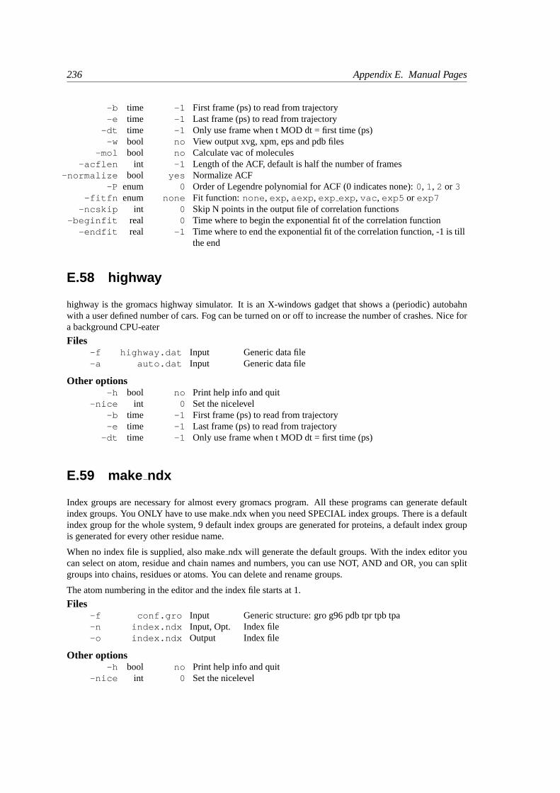
236 Appendix E. Manual Pages
-b time -1 First frame (ps) to read from trajectory-e time -1 Last frame (ps) to read from trajectory
-dt time -1 Only use frame when t MOD dt = first time (ps)-w bool no View output xvg, xpm, eps and pdb files
-mol bool no Calculate vac of molecules-acflen int -1 Length of the ACF, default is half the number of frames
-normalize bool yes Normalize ACF-P enum 0 Order of Legendre polynomial for ACF (0 indicates none):0, 1, 2 or 3
-fitfn enum none Fit function: none , exp , aexp , exp exp , vac , exp5 or exp7-ncskip int 0 Skip N points in the output file of correlation functions
-beginfit real 0 Time where to begin the exponential fit of the correlation function-endfit real -1 Time where to end the exponential fit of the correlation function, -1 is till
the end
E.58 highway
highway is the gromacs highway simulator. It is an X-windows gadget that shows a (periodic) autobahnwith a user defined number of cars. Fog can be turned on or off to increase the number of crashes. Nice fora background CPU-eater
Files-f highway.dat Input Generic data file-a auto.dat Input Generic data file
Other options-h bool no Print help info and quit
-nice int 0 Set the nicelevel-b time -1 First frame (ps) to read from trajectory-e time -1 Last frame (ps) to read from trajectory
-dt time -1 Only use frame when t MOD dt = first time (ps)
E.59 make ndx
Index groups are necessary for almost every gromacs program. All these programs can generate defaultindex groups. You ONLY have to use makendx when you need SPECIAL index groups. There is a defaultindex group for the whole system, 9 default index groups are generated for proteins, a default index groupis generated for every other residue name.
When no index file is supplied, also makendx will generate the default groups. With the index editor youcan select on atom, residue and chain names and numbers, you can use NOT, AND and OR, you can splitgroups into chains, residues or atoms. You can delete and rename groups.
The atom numbering in the editor and the index file starts at 1.
Files-f conf.gro Input Generic structure: gro g96 pdb tpr tpb tpa-n index.ndx Input, Opt. Index file-o index.ndx Output Index file
Other options-h bool no Print help info and quit
-nice int 0 Set the nicelevel
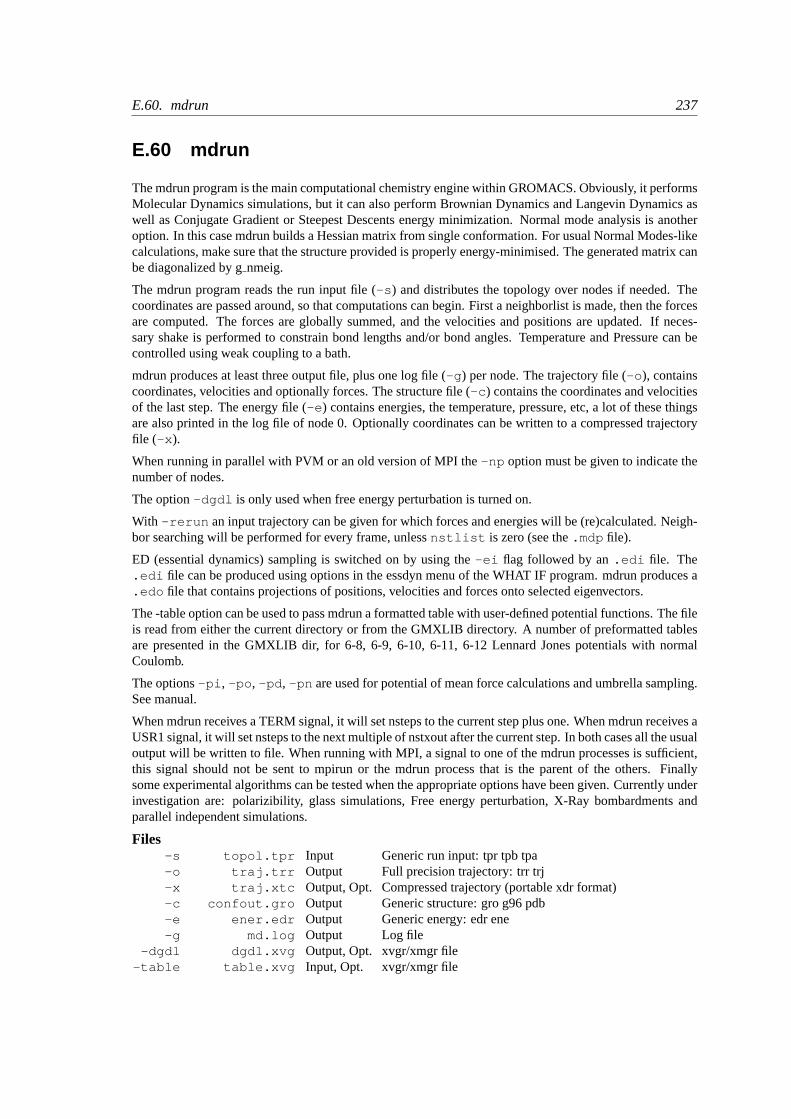
E.60. mdrun 237
E.60 mdrun
The mdrun program is the main computational chemistry engine within GROMACS. Obviously, it performsMolecular Dynamics simulations, but it can also perform Brownian Dynamics and Langevin Dynamics aswell as Conjugate Gradient or Steepest Descents energy minimization. Normal mode analysis is anotheroption. In this case mdrun builds a Hessian matrix from single conformation. For usual Normal Modes-likecalculations, make sure that the structure provided is properly energy-minimised. The generated matrix canbe diagonalized by gnmeig.
The mdrun program reads the run input file (-s ) and distributes the topology over nodes if needed. Thecoordinates are passed around, so that computations can begin. First a neighborlist is made, then the forcesare computed. The forces are globally summed, and the velocities and positions are updated. If neces-sary shake is performed to constrain bond lengths and/or bond angles. Temperature and Pressure can becontrolled using weak coupling to a bath.
mdrun produces at least three output file, plus one log file (-g ) per node. The trajectory file (-o ), containscoordinates, velocities and optionally forces. The structure file (-c ) contains the coordinates and velocitiesof the last step. The energy file (-e ) contains energies, the temperature, pressure, etc, a lot of these thingsare also printed in the log file of node 0. Optionally coordinates can be written to a compressed trajectoryfile (-x ).
When running in parallel with PVM or an old version of MPI the-np option must be given to indicate thenumber of nodes.
The option-dgdl is only used when free energy perturbation is turned on.
With -rerun an input trajectory can be given for which forces and energies will be (re)calculated. Neigh-bor searching will be performed for every frame, unlessnstlist is zero (see the.mdp file).
ED (essential dynamics) sampling is switched on by using the-ei flag followed by an.edi file. The.edi file can be produced using options in the essdyn menu of the WHAT IF program. mdrun produces a.edo file that contains projections of positions, velocities and forces onto selected eigenvectors.
The -table option can be used to pass mdrun a formatted table with user-defined potential functions. The fileis read from either the current directory or from the GMXLIB directory. A number of preformatted tablesare presented in the GMXLIB dir, for 6-8, 6-9, 6-10, 6-11, 6-12 Lennard Jones potentials with normalCoulomb.
The options-pi , -po , -pd , -pn are used for potential of mean force calculations and umbrella sampling.See manual.
When mdrun receives a TERM signal, it will set nsteps to the current step plus one. When mdrun receives aUSR1 signal, it will set nsteps to the next multiple of nstxout after the current step. In both cases all the usualoutput will be written to file. When running with MPI, a signal to one of the mdrun processes is sufficient,this signal should not be sent to mpirun or the mdrun process that is the parent of the others. Finallysome experimental algorithms can be tested when the appropriate options have been given. Currently underinvestigation are: polarizibility, glass simulations, Free energy perturbation, X-Ray bombardments andparallel independent simulations.
Files-s topol.tpr Input Generic run input: tpr tpb tpa-o traj.trr Output Full precision trajectory: trr trj-x traj.xtc Output, Opt. Compressed trajectory (portable xdr format)-c confout.gro Output Generic structure: gro g96 pdb-e ener.edr Output Generic energy: edr ene-g md.log Output Log file
-dgdl dgdl.xvg Output, Opt. xvgr/xmgr file-table table.xvg Input, Opt. xvgr/xmgr file
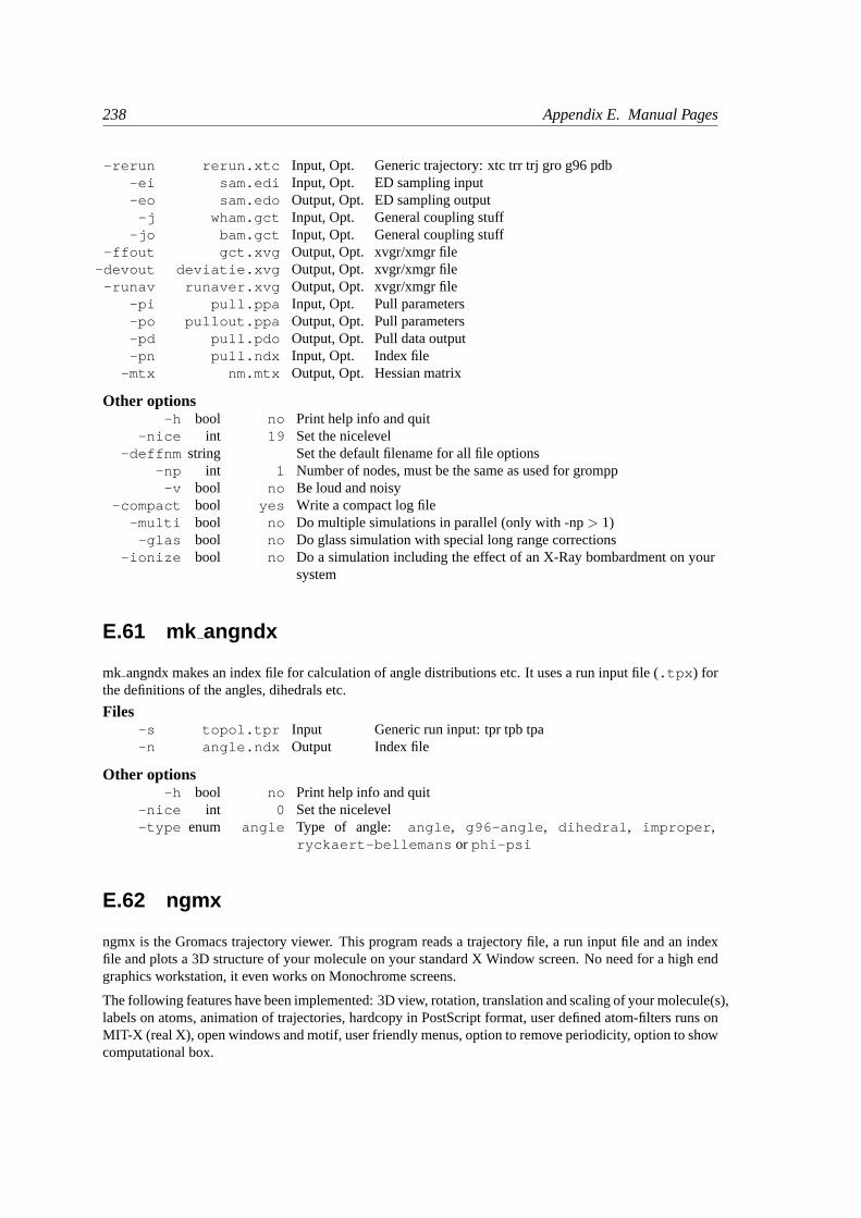
238 Appendix E. Manual Pages
-rerun rerun.xtc Input, Opt. Generic trajectory: xtc trr trj gro g96 pdb-ei sam.edi Input, Opt. ED sampling input-eo sam.edo Output, Opt. ED sampling output
-j wham.gct Input, Opt. General coupling stuff-jo bam.gct Input, Opt. General coupling stuff
-ffout gct.xvg Output, Opt. xvgr/xmgr file-devout deviatie.xvg Output, Opt. xvgr/xmgr file
-runav runaver.xvg Output, Opt. xvgr/xmgr file-pi pull.ppa Input, Opt. Pull parameters-po pullout.ppa Output, Opt. Pull parameters-pd pull.pdo Output, Opt. Pull data output-pn pull.ndx Input, Opt. Index file
-mtx nm.mtx Output, Opt. Hessian matrix
Other options-h bool no Print help info and quit
-nice int 19 Set the nicelevel-deffnm string Set the default filename for all file options
-np int 1 Number of nodes, must be the same as used for grompp-v bool no Be loud and noisy
-compact bool yes Write a compact log file-multi bool no Do multiple simulations in parallel (only with -np> 1)
-glas bool no Do glass simulation with special long range corrections-ionize bool no Do a simulation including the effect of an X-Ray bombardment on your
system
E.61 mk angndx
mk angndx makes an index file for calculation of angle distributions etc. It uses a run input file (.tpx ) forthe definitions of the angles, dihedrals etc.
Files-s topol.tpr Input Generic run input: tpr tpb tpa-n angle.ndx Output Index file
Other options-h bool no Print help info and quit
-nice int 0 Set the nicelevel-type enum angle Type of angle: angle , g96-angle , dihedral , improper ,
ryckaert-bellemans or phi-psi
E.62 ngmx
ngmx is the Gromacs trajectory viewer. This program reads a trajectory file, a run input file and an indexfile and plots a 3D structure of your molecule on your standard X Window screen. No need for a high endgraphics workstation, it even works on Monochrome screens.
The following features have been implemented: 3D view, rotation, translation and scaling of your molecule(s),labels on atoms, animation of trajectories, hardcopy in PostScript format, user defined atom-filters runs onMIT-X (real X), open windows and motif, user friendly menus, option to remove periodicity, option to showcomputational box.
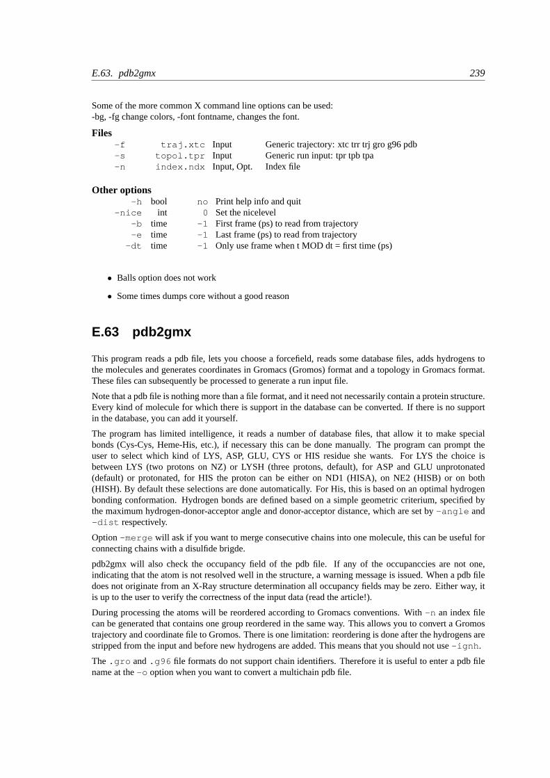
E.63. pdb2gmx 239
Some of the more common X command line options can be used:-bg, -fg change colors, -font fontname, changes the font.
Files-f traj.xtc Input Generic trajectory: xtc trr trj gro g96 pdb-s topol.tpr Input Generic run input: tpr tpb tpa-n index.ndx Input, Opt. Index file
Other options-h bool no Print help info and quit
-nice int 0 Set the nicelevel-b time -1 First frame (ps) to read from trajectory-e time -1 Last frame (ps) to read from trajectory
-dt time -1 Only use frame when t MOD dt = first time (ps)
• Balls option does not work
• Some times dumps core without a good reason
E.63 pdb2gmx
This program reads a pdb file, lets you choose a forcefield, reads some database files, adds hydrogens tothe molecules and generates coordinates in Gromacs (Gromos) format and a topology in Gromacs format.These files can subsequently be processed to generate a run input file.
Note that a pdb file is nothing more than a file format, and it need not necessarily contain a protein structure.Every kind of molecule for which there is support in the database can be converted. If there is no supportin the database, you can add it yourself.
The program has limited intelligence, it reads a number of database files, that allow it to make specialbonds (Cys-Cys, Heme-His, etc.), if necessary this can be done manually. The program can prompt theuser to select which kind of LYS, ASP, GLU, CYS or HIS residue she wants. For LYS the choice isbetween LYS (two protons on NZ) or LYSH (three protons, default), for ASP and GLU unprotonated(default) or protonated, for HIS the proton can be either on ND1 (HISA), on NE2 (HISB) or on both(HISH). By default these selections are done automatically. For His, this is based on an optimal hydrogenbonding conformation. Hydrogen bonds are defined based on a simple geometric criterium, specified bythe maximum hydrogen-donor-acceptor angle and donor-acceptor distance, which are set by-angle and-dist respectively.
Option-merge will ask if you want to merge consecutive chains into one molecule, this can be useful forconnecting chains with a disulfide brigde.
pdb2gmx will also check the occupancy field of the pdb file. If any of the occupanccies are not one,indicating that the atom is not resolved well in the structure, a warning message is issued. When a pdb filedoes not originate from an X-Ray structure determination all occupancy fields may be zero. Either way, itis up to the user to verify the correctness of the input data (read the article!).
During processing the atoms will be reordered according to Gromacs conventions. With-n an index filecan be generated that contains one group reordered in the same way. This allows you to convert a Gromostrajectory and coordinate file to Gromos. There is one limitation: reordering is done after the hydrogens arestripped from the input and before new hydrogens are added. This means that you should not use-ignh .
The .gro and.g96 file formats do not support chain identifiers. Therefore it is useful to enter a pdb filename at the-o option when you want to convert a multichain pdb file.
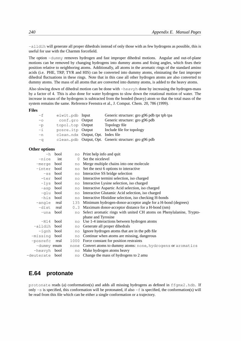
240 Appendix E. Manual Pages
-alldih will generate all proper dihedrals instead of only those with as few hydrogens as possible, this isuseful for use with the Charmm forcefield.
The option-dummy removes hydrogen and fast improper dihedral motions. Angular and out-of-planemotions can be removed by changing hydrogens into dummy atoms and fixing angles, which fixes theirposition relative to neighboring atoms. Additionally, all atoms in the aromatic rings of the standard aminoacids (i.e. PHE, TRP, TYR and HIS) can be converted into dummy atoms, elminating the fast improperdihedral fluctuations in these rings. Note that in this case all other hydrogen atoms are also converted todummy atoms. The mass of all atoms that are converted into dummy atoms, is added to the heavy atoms.
Also slowing down of dihedral motion can be done with-heavyh done by increasing the hydrogen-massby a factor of 4. This is also done for water hydrogens to slow down the rotational motion of water. Theincrease in mass of the hydrogens is subtracted from the bonded (heavy) atom so that the total mass of thesystem remains the same. Reference Feenstra et al., J. Comput. Chem. 20, 786 (1999).
Files-f eiwit.pdb Input Generic structure: gro g96 pdb tpr tpb tpa-o conf.gro Output Generic structure: gro g96 pdb-p topol.top Output Topology file-i posre.itp Output Include file for topology-n clean.ndx Output, Opt. Index file-q clean.pdb Output, Opt. Generic structure: gro g96 pdb
Other options-h bool no Print help info and quit
-nice int 0 Set the nicelevel-merge bool no Merge multiple chains into one molecule-inter bool no Set the next 6 options to interactive
-ss bool no Interactive SS bridge selection-ter bool no Interactive termini selection, iso charged-lys bool no Interactive Lysine selection, iso charged-asp bool no Interactive Aspartic Acid selection, iso charged-glu bool no Interactive Glutamic Acid selection, iso charged-his bool no Interactive Histidine selection, iso checking H-bonds
-angle real 135 Minimum hydrogen-donor-acceptor angle for a H-bond (degrees)-dist real 0.3 Maximum donor-acceptor distance for a H-bond (nm)
-una bool no Select aromatic rings with united CH atoms on Phenylalanine, Trypto-phane and Tyrosine
-H14 bool no Use 1-4 interactions between hydrogen atoms-alldih bool no Generate all proper dihedrals
-ignh bool no Ignore hydrogen atoms that are in the pdb file-missing bool no Continue when atoms are missing, dangerous-posrefc real 1000 Force constant for position restraints
-dummy enum none Convert atoms to dummy atoms:none , hydrogens or aromatics-heavyh bool no Make hydrogen atoms heavy
-deuterate bool no Change the mass of hydrogens to 2 amu
E.64 protonate
protonate reads (a) conformation(s) and adds all missing hydrogens as defined inffgmx2.hdb . Ifonly -s is specified, this conformation will be protonated, if also-f is specified, the conformation(s) willbe read from this file which can be either a single conformation or a trajectory.
E.65. tpbconv 241
If a pdb file is supplied, residue names might not correspond to to the GROMACS naming conventions, inwhich case these residues will probably not be properly protonated.
If an index file is specified, please note that the atom numbers should correspond to theprotonated state.Files
-s topol.tpr Input Structure+mass(db): tpr tpb tpa gro g96 pdb-f traj.xtc Input, Opt. Generic trajectory: xtc trr trj gro g96 pdb-n index.ndx Input, Opt. Index file-o protonated.xtc Output Generic trajectory: xtc trr trj gro g96 pdb
Other options-h bool no Print help info and quit
-nice int 0 Set the nicelevel-b time -1 First frame (ps) to read from trajectory-e time -1 Last frame (ps) to read from trajectory
-dt time -1 Only use frame when t MOD dt = first time (ps)
E.65 tpbconv
tpbconv can edit run input files in three ways.
1st. by creating a run input file for a continuation run when your simulation has crashed due to e.g. a fulldisk, or by making a continuation run input file. Note that a frame with coordinates and velocities is needed,which means that when you never write velocities, you can not use tpbconv and you have to start the runagain from the beginning.
2nd. by creating a tpx file for a subset of your original tpx file, which is useful when you want to removethe solvent from your tpx file, or when you want to make e.g. a pure Ca tpx file.WARNING: this tpx fileis not fully functional . 3rd. by setting the charges of a specified group to zero. This is useful when doingfree energy estimates using the LIE (Linear Interactio Energy) method.Files
-s topol.tpr Input Generic run input: tpr tpb tpa-f traj.trr Input, Opt. Full precision trajectory: trr trj-n index.ndx Input, Opt. Index file-o tpxout.tpr Output Generic run input: tpr tpb tpa
Other options-h bool no Print help info and quit
-nice int 0 Set the nicelevel-time real -1 Continue from frame at this time (ps) instead of the last frame
-extend real 0 Extend runtime by this amount (ps)-until real 0 Extend runtime until this ending time (ps)-zeroq bool no Set the charges of a group (from the index) to zero
-unconstrained bool yes For a continuous trajectory, the constraints should not be solved beforethe first step (default)
E.66 trjcat
trjcat concatenates several input trajectory files in sorted order. In case of double time frames the one inthe later file is used. By specifying-settime you will be asked for the start time of each file. The inputfiles are taken from the command line, such that a command liketrjcat -o fixed.trr *.trrshould do the trick. Using-cat you can simply paste several files together without removal of frames withidentical time stamps.
242 Appendix E. Manual Pages
Files-o trajout.xtc Output Generic trajectory: xtc trr trj gro g96 pdb-n index.ndx Input, Opt. Index file
Other options-h bool no Print help info and quit
-nice int 19 Set the nicelevel-tu enum ps Time unit: ps , fs , ns , us , ms, s , mor h
-b time -1 First time to use (ps)-e time -1 Last time to use (ps)
-dt time 0 Only write frame when t MOD dt = first time (ps)-prec int 3 Precision for .xtc and .gro writing in number of decimal places
-vel bool yes Read and write velocities if possible-settime bool no Change starting time interactively
-sort bool yes Sort trajectory files (not frames)-cat bool no do not discard double time frames
E.67 trjconv
trjconv can convert trajectory files in many ways:1. from one format to another2. select a subset of atoms3. remove periodicity from molecules4. keep multimeric molecules together5. center atoms in the box6. fit atoms to reference structure7. reduce the number of frames8. change the timestamps of the frames (-t0 and-timestep )
The programtrjcat can concatenate multiple trajectory files.
Currently seven formats are supported for input and output:.xtc , .trr , .trj , .gro , .g96 , .pdb and.g87 . The file formats are detected from the file extension. The precision of.xtc and.gro output istaken from the input file for.xtc , .gro and.pdb , and from the-ndec option for other input formats.The precision is always taken from-ndec , when this option is set. All other formats have fixed precision..trr and.trj output can be single or double precision, depending on the precision of the trjconv binary.Note that velocities are only supported in.trr , .trj , .gro and.g96 files.
Option-app can be used to append output to an existing trajectory file. No checks are performed to ensureintegrity of the resulting combined trajectory file.
Option -sep can be used to write every frame to a seperate .gro, .g96 or .pdb file, default all frames allwritten to one file..pdb files with all frames concatenated can be viewed withrasmol -nmrpdb .
It is possible to select part of your trajectory and write it out to a new trajectory file in order to save diskspace, e.g. for leaving out the water from a trajectory of a protein in water.ALWAYS put the originaltrajectory on tape! We recommend to use the portable.xtc format for your analysis to save disk spaceand to have portable files.
There are two options for fitting the trajectory to a reference either for essential dynamics analysis or forwhatever. The first option is just plain fitting to a reference structure in the structure file, the second optionis a progressive fit in which the first timeframe is fitted to the reference structure in the structure file toobtain and each subsequent timeframe is fitted to the previously fitted structure. This way a continuoustrajectory is generated, which might not be the case when using the regular fit method, e.g. when yourprotein undergoes large conformational transitions.
E.67. trjconv 243
Option -pbc sets the type of periodic boundary condition treatment.whole puts the atoms in the boxand then makes broken molecules whole (a run input file is required).inbox puts all the atoms in thebox. nojump checks if atoms jump across the box and then puts them back. This has the effect that allmolecules will remain whole (provided they were whole in the initial conformation), note that this ensures acontinuous trajectory but molecules may diffuse out of the box. The starting configuration for this procedureis taken from the structure file, if one is supplied, otherwise it is the first frame.-pbc is ignored when-fitof -pfit is set, in that case molecules will be made whole.
Option-ur sets the unit cell representation for optionswhole andinbox of -pbc . All three options givedifferent results for triclinc boxes and identical results for rectangular boxes.rect is the ordinary brickshape.tric is the triclinic unit cell.compact puts all atoms at the closest distance from the center of thebox. This can be useful for visualizing e.g. truncated octahedrons.
Option -center centers the system in the box. The user can select the group which is used to determinethe geometrical center. Use option-pbc whole in addition to-center when you want all moleculesin the box after the centering.
With -dt it is possible to reduce the number of frames in the output. This option relies on the accuracy ofthe times in your input trajectory, so if these are inaccurate use the-timestep option to modify the time(this can be done simultaneously).
Using-trunc trjconv can truncate.trj in place, i.e. without copying the file. This is useful when a runhas crashed during disk I/O (one more disk full), or when two contiguous trajectories must be concatenatedwithout have double frames.
trjcat is more suitable for concatenating trajectory files.
Option-dump can be used to extract a frame at or near one specific time from your trajectory.
Files-f traj.xtc Input Generic trajectory: xtc trr trj gro g96 pdb-o trajout.xtc Output Generic trajectory: xtc trr trj gro g96 pdb-s topol.tpr Input, Opt. Structure+mass(db): tpr tpb tpa gro g96 pdb-n index.ndx Input, Opt. Index file
-fr frames.ndx Input, Opt. Index file
Other options-h bool no Print help info and quit
-nice int 19 Set the nicelevel-b time -1 First frame (ps) to read from trajectory-e time -1 Last frame (ps) to read from trajectory
-tu enum ps Time unit: ps , fs , ns , us , ms, s , mor h-w bool no View output xvg, xpm, eps and pdb files
-skip int 1 Only write every nr-th frame-dt time 0 Only write frame when t MOD dt = first time (ps)
-dump time -1 Dump frame nearest specified time (ps)-t0 time 0 Starting time (ps) (default: don’t change)
-timestep time 0 Change time step between input frames (ps)-pbc enum none PBC treatment:none , whole , inbox or nojump
-ur enum rect Unit-cell representation:rect , tric or compact-center bool no Center atoms in box
-box vector 0 0 0 Size for new cubic box (default: read from input)-shift vector 0 0 0 All coordinates will be shifted by framenr*shift
-fit bool no Fit molecule to ref structure in the structure file-pfit bool no Progressive fit, to the previous fitted structure-ndec int 3 Precision for .xtc and .gro writing in number of decimal places
-vel bool yes Read and write velocities if possible
244 Appendix E. Manual Pages
-force bool no Read and write forces if possible-trunc time -1 Truncate input trj file after this time (ps)
-exec string Execute command for every output frame with the frame number as ar-gument
-app bool no Append output-split time 0 Start writing new file when t MOD split = first time (ps)
-sep bool no Write each frame to a separate .gro, .g96 or .pdb file
E.68 trjorder
trjorder orders molecules according to the smallest distance to atoms in a reference group. It will ask for agroup of reference atoms and a group of molecules. For each frame of the trajectory the selected moleculeswill be reordered according to the shortest distance between atom number-da in the molecule and all theatoms in the reference group. All atoms in the trajectory are written to the output trajectory.
trjorder can be useful for e.g. analyzing the n waters closest to a protein. In that case the reference groupwould be the protein and the group of molecules would consist of all the water atoms. When an index groupof the first n waters is made, the ordered trajectory can be used with any Gromacs program to analyze the nclosest waters.
Files-f traj.xtc Input Generic trajectory: xtc trr trj gro g96 pdb-s topol.tpr Input Structure+mass(db): tpr tpb tpa gro g96 pdb-n index.ndx Input, Opt. Index file-o ordered.xtc Output Generic trajectory: xtc trr trj gro g96 pdb
Other options-h bool no Print help info and quit
-nice int 19 Set the nicelevel-b time -1 First frame (ps) to read from trajectory-e time -1 Last frame (ps) to read from trajectory
-dt time -1 Only use frame when t MOD dt = first time (ps)-na int 3 Number of atoms in a molecule-da int 1 Atom used for the distance calculation
E.69 wheel
wheel plots a helical wheel representation of your sequence.The input sequence is in the .dat file where thefirst line contains the number of residues and each consecutive line contains a residuename.
Files-f nnnice.dat Input Generic data file-o plot.eps Output Encapsulated PostScript (tm) file
Other options-h bool no Print help info and quit
-nice int 19 Set the nicelevel-r0 int 1 The first residue number in the sequence
-rot0 real 0 Rotate around an angle initially (90 degrees makes sense)-T string Plot a title in the center of the wheel (must be shorter than 10 characters,
or it will overwrite the wheel)-nn bool yes Toggle numbers
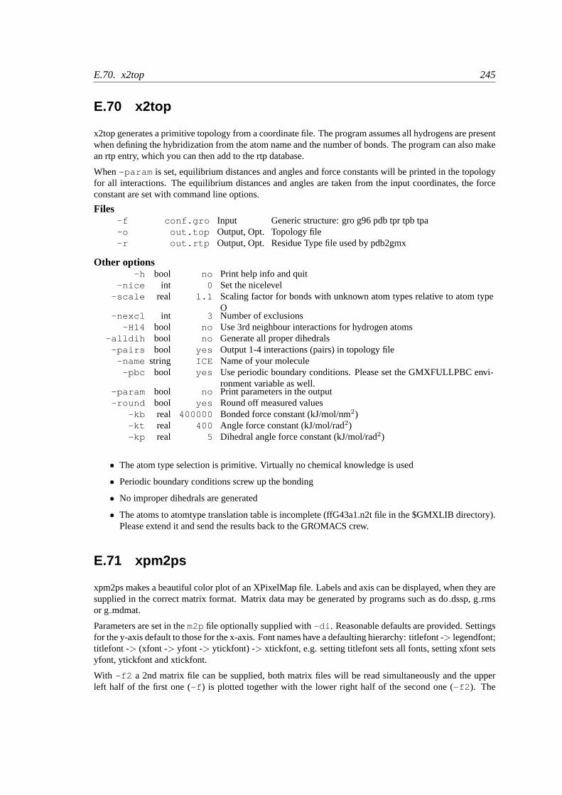
E.70. x2top 245
E.70 x2top
x2top generates a primitive topology from a coordinate file. The program assumes all hydrogens are presentwhen defining the hybridization from the atom name and the number of bonds. The program can also makean rtp entry, which you can then add to the rtp database.
When-param is set, equilibrium distances and angles and force constants will be printed in the topologyfor all interactions. The equilibrium distances and angles are taken from the input coordinates, the forceconstant are set with command line options.
Files-f conf.gro Input Generic structure: gro g96 pdb tpr tpb tpa-o out.top Output, Opt. Topology file-r out.rtp Output, Opt. Residue Type file used by pdb2gmx
Other options-h bool no Print help info and quit
-nice int 0 Set the nicelevel-scale real 1.1 Scaling factor for bonds with unknown atom types relative to atom type
O-nexcl int 3 Number of exclusions
-H14 bool no Use 3rd neighbour interactions for hydrogen atoms-alldih bool no Generate all proper dihedrals
-pairs bool yes Output 1-4 interactions (pairs) in topology file-name string ICE Name of your molecule
-pbc bool yes Use periodic boundary conditions. Please set the GMXFULLPBC envi-ronment variable as well.
-param bool no Print parameters in the output-round bool yes Round off measured values
-kb real 400000 Bonded force constant (kJ/mol/nm2)-kt real 400 Angle force constant (kJ/mol/rad2)-kp real 5 Dihedral angle force constant (kJ/mol/rad2)
• The atom type selection is primitive. Virtually no chemical knowledge is used
• Periodic boundary conditions screw up the bonding
• No improper dihedrals are generated
• The atoms to atomtype translation table is incomplete (ffG43a1.n2t file in the $GMXLIB directory).Please extend it and send the results back to the GROMACS crew.
E.71 xpm2ps
xpm2ps makes a beautiful color plot of an XPixelMap file. Labels and axis can be displayed, when they aresupplied in the correct matrix format. Matrix data may be generated by programs such as dodssp, grmsor g mdmat.
Parameters are set in them2pfile optionally supplied with-di . Reasonable defaults are provided. Settingsfor the y-axis default to those for the x-axis. Font names have a defaulting hierarchy: titlefont -> legendfont;titlefont -> (xfont -> yfont -> ytickfont) -> xtickfont, e.g. setting titlefont sets all fonts, setting xfont setsyfont, ytickfont and xtickfont.
With -f2 a 2nd matrix file can be supplied, both matrix files will be read simultaneously and the upperleft half of the first one (-f ) is plotted together with the lower right half of the second one (-f2 ). The
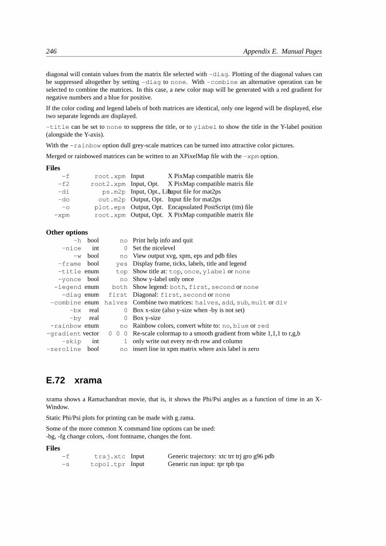
246 Appendix E. Manual Pages
diagonal will contain values from the matrix file selected with-diag . Plotting of the diagonal values canbe suppressed altogether by setting-diag to none . With -combine an alternative operation can beselected to combine the matrices. In this case, a new color map will be generated with a red gradient fornegative numbers and a blue for positive.
If the color coding and legend labels of both matrices are identical, only one legend will be displayed, elsetwo separate legends are displayed.
-title can be set tonone to suppress the title, or toylabel to show the title in the Y-label position(alongside the Y-axis).
With the-rainbow option dull grey-scale matrices can be turned into attractive color pictures.
Merged or rainbowed matrices can be written to an XPixelMap file with the-xpm option.
Files-f root.xpm Input X PixMap compatible matrix file
-f2 root2.xpm Input, Opt. X PixMap compatible matrix file-di ps.m2p Input, Opt., Lib.Input file for mat2ps-do out.m2p Output, Opt. Input file for mat2ps
-o plot.eps Output, Opt. Encapsulated PostScript (tm) file-xpm root.xpm Output, Opt. X PixMap compatible matrix file
Other options-h bool no Print help info and quit
-nice int 0 Set the nicelevel-w bool no View output xvg, xpm, eps and pdb files
-frame bool yes Display frame, ticks, labels, title and legend-title enum top Show title at:top , once , ylabel or none-yonce bool no Show y-label only once
-legend enum both Show legend:both , first , second or none-diag enum first Diagonal:first , second or none
-combine enum halves Combine two matrices:halves , add , sub , mult or div-bx real 0 Box x-size (also y-size when -by is not set)-by real 0 Box y-size
-rainbow enum no Rainbow colors, convert white to:no , blue or red-gradient vector 0 0 0 Re-scale colormap to a smooth gradient from white 1,1,1 to r,g,b
-skip int 1 only write out every nr-th row and column-zeroline bool no insert line in xpm matrix where axis label is zero
E.72 xrama
xrama shows a Ramachandran movie, that is, it shows the Phi/Psi angles as a function of time in an X-Window.
Static Phi/Psi plots for printing can be made with grama.
Some of the more common X command line options can be used:-bg, -fg change colors, -font fontname, changes the font.
Files-f traj.xtc Input Generic trajectory: xtc trr trj gro g96 pdb-s topol.tpr Input Generic run input: tpr tpb tpa

E.72. xrama 247
Other options-h bool no Print help info and quit
-nice int 0 Set the nicelevel-b time -1 First frame (ps) to read from trajectory-e time -1 Last frame (ps) to read from trajectory
-dt time -1 Only use frame when t MOD dt = first time (ps)

248 Appendix E. Manual Pages
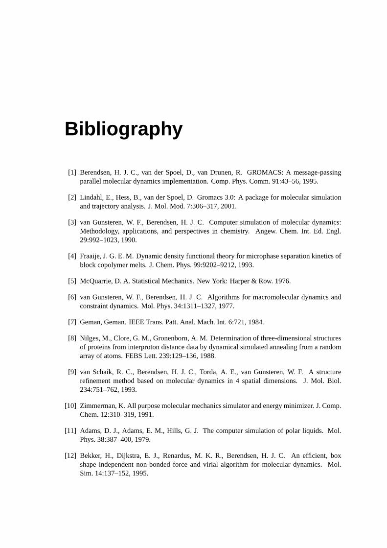
Bibliography
[1] Berendsen, H. J. C., van der Spoel, D., van Drunen, R. GROMACS: A message-passingparallel molecular dynamics implementation. Comp. Phys. Comm. 91:43–56, 1995.
[2] Lindahl, E., Hess, B., van der Spoel, D. Gromacs 3.0: A package for molecular simulationand trajectory analysis. J. Mol. Mod. 7:306–317, 2001.
[3] van Gunsteren, W. F., Berendsen, H. J. C. Computer simulation of molecular dynamics:Methodology, applications, and perspectives in chemistry. Angew. Chem. Int. Ed. Engl.29:992–1023, 1990.
[4] Fraaije, J. G. E. M. Dynamic density functional theory for microphase separation kinetics ofblock copolymer melts. J. Chem. Phys. 99:9202–9212, 1993.
[5] McQuarrie, D. A. Statistical Mechanics. New York: Harper & Row. 1976.
[6] van Gunsteren, W. F., Berendsen, H. J. C. Algorithms for macromolecular dynamics andconstraint dynamics. Mol. Phys. 34:1311–1327, 1977.
[7] Geman, Geman. IEEE Trans. Patt. Anal. Mach. Int. 6:721, 1984.
[8] Nilges, M., Clore, G. M., Gronenborn, A. M. Determination of three-dimensional structuresof proteins from interproton distance data by dynamical simulated annealing from a randomarray of atoms. FEBS Lett. 239:129–136, 1988.
[9] van Schaik, R. C., Berendsen, H. J. C., Torda, A. E., van Gunsteren, W. F. A structurerefinement method based on molecular dynamics in 4 spatial dimensions. J. Mol. Biol.234:751–762, 1993.
[10] Zimmerman, K. All purpose molecular mechanics simulator and energy minimizer. J. Comp.Chem. 12:310–319, 1991.
[11] Adams, D. J., Adams, E. M., Hills, G. J. The computer simulation of polar liquids. Mol.Phys. 38:387–400, 1979.
[12] Bekker, H., Dijkstra, E. J., Renardus, M. K. R., Berendsen, H. J. C. An efficient, boxshape independent non-bonded force and virial algorithm for molecular dynamics. Mol.Sim. 14:137–152, 1995.
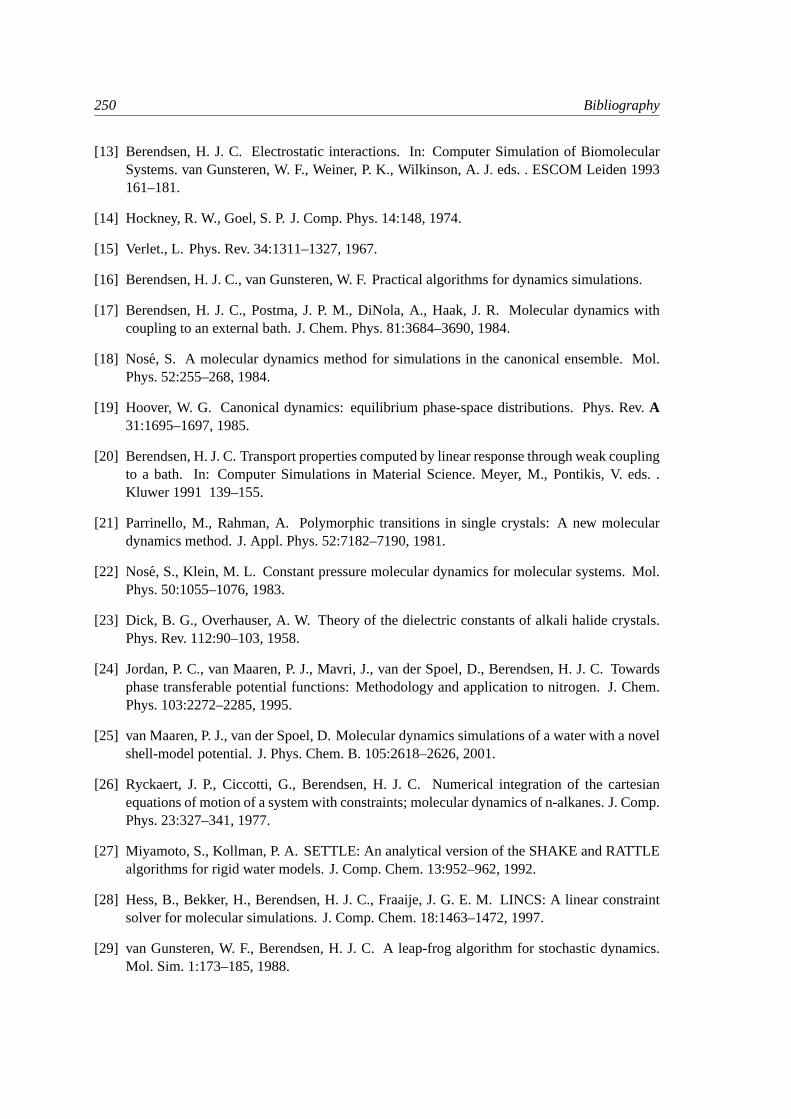
250 Bibliography
[13] Berendsen, H. J. C. Electrostatic interactions. In: Computer Simulation of BiomolecularSystems. van Gunsteren, W. F., Weiner, P. K., Wilkinson, A. J. eds. . ESCOM Leiden 1993161–181.
[14] Hockney, R. W., Goel, S. P. J. Comp. Phys. 14:148, 1974.
[15] Verlet., L. Phys. Rev. 34:1311–1327, 1967.
[16] Berendsen, H. J. C., van Gunsteren, W. F. Practical algorithms for dynamics simulations.
[17] Berendsen, H. J. C., Postma, J. P. M., DiNola, A., Haak, J. R. Molecular dynamics withcoupling to an external bath. J. Chem. Phys. 81:3684–3690, 1984.
[18] Nose, S. A molecular dynamics method for simulations in the canonical ensemble. Mol.Phys. 52:255–268, 1984.
[19] Hoover, W. G. Canonical dynamics: equilibrium phase-space distributions. Phys. Rev.A31:1695–1697, 1985.
[20] Berendsen, H. J. C. Transport properties computed by linear response through weak couplingto a bath. In: Computer Simulations in Material Science. Meyer, M., Pontikis, V. eds. .Kluwer 1991 139–155.
[21] Parrinello, M., Rahman, A. Polymorphic transitions in single crystals: A new moleculardynamics method. J. Appl. Phys. 52:7182–7190, 1981.
[22] Nose, S., Klein, M. L. Constant pressure molecular dynamics for molecular systems. Mol.Phys. 50:1055–1076, 1983.
[23] Dick, B. G., Overhauser, A. W. Theory of the dielectric constants of alkali halide crystals.Phys. Rev. 112:90–103, 1958.
[24] Jordan, P. C., van Maaren, P. J., Mavri, J., van der Spoel, D., Berendsen, H. J. C. Towardsphase transferable potential functions: Methodology and application to nitrogen. J. Chem.Phys. 103:2272–2285, 1995.
[25] van Maaren, P. J., van der Spoel, D. Molecular dynamics simulations of a water with a novelshell-model potential. J. Phys. Chem. B. 105:2618–2626, 2001.
[26] Ryckaert, J. P., Ciccotti, G., Berendsen, H. J. C. Numerical integration of the cartesianequations of motion of a system with constraints; molecular dynamics of n-alkanes. J. Comp.Phys. 23:327–341, 1977.
[27] Miyamoto, S., Kollman, P. A. SETTLE: An analytical version of the SHAKE and RATTLEalgorithms for rigid water models. J. Comp. Chem. 13:952–962, 1992.
[28] Hess, B., Bekker, H., Berendsen, H. J. C., Fraaije, J. G. E. M. LINCS: A linear constraintsolver for molecular simulations. J. Comp. Chem. 18:1463–1472, 1997.
[29] van Gunsteren, W. F., Berendsen, H. J. C. A leap-frog algorithm for stochastic dynamics.Mol. Sim. 1:173–185, 1988.
Bibliography 251
[30] Levitt, M., Sander, C., Stern, P. S. The normal modes of a protein: Native bovine pancreatictrypsin inhibitor. Proc. Natl. Acad. Sci. USA 10:181–199, 1983.
[31] Go, N., Noguti, T., Nishikawa, T. Dynamics of a small globular protein in terms of low-frequency vibrational modes. Proc. Natl. Acad. Sci. USA 80:3696–3700, 1983.
[32] Brooks, B., Karplus, M. Harmonic dynamics of proteins: Normal modes and fluctuations inbovine pancreatic trypsin inhibitor. Proc. Natl. Acad. Sci. USA 80:6571–6575, 1983.
[33] Hayward, S., Go, N. Collective variable description of native protein dynamics. Annu. Rev.Phys. Chem. 46:223–250, 1995.
[34] de Groot, B. L., Amadei, A., van Aalten, D. M. F., Berendsen, H. J. C. Towards an exhaustivesampling of the configurational spaces of the two forms of the peptide hormone guanylin. J.Biomol. Str. Dyn. 13(5):741–751, 1996.
[35] de Groot, B. L., Amadei, A., Scheek, R. M., van Nuland, N. A. J., Berendsen, H. J. C.An extended sampling of the configurational space of hpr frome. coli. PROTEINS: Struct.Funct. Gen. 26:314–322, 1996.
[36] Vriend, G. WHAT IF: a molecular modeling and drug design program. J. Mol. Graph.8:52–56, 1990.
[37] Fincham, D. Parallel computers and molecular simulation. Mol. Sim. 1:1, 1987.
[38] Raine, A. R. C., Fincham, D., Smith, W. Systolic loop methods for molecular dynamicssimulation. Comp. Phys. Comm. 55:13–30, 1989.
[39] van Gunsteren, W. F., Berendsen, H. J. C. Gromos-87 manual. Biomos BV Nijenborgh 4,9747 AG Groningen, The Netherlands 1987.
[40] van Buuren, A. R., Marrink, S. J., Berendsen, H. J. C. A molecular dynamics study of thedecane/water interface. J. Phys. Chem. 97:9206–9212, 1993.
[41] Mark, A. E., van Helden, S. P., Smith, P. E., Janssen, L. H. M., van Gunsteren, W. F. Con-vergence properties of free energy calculations:α-cyclodextrin complexes as a case study. J.Am. Chem. Soc. 116:6293–6302, 1994.
[42] Jorgensen, W. L., Chandrasekhar, J., Madura, J. D., Impey, R. W., Klein, M. L. Comparisonof simple potential functions for simulating liquid water. J. Chem. Phys. 79:926–935, 1983.
[43] van Buuren, A. R., Berendsen, H. J. C. Molecular dynamics simulation of the stability ofa 22 residue alpha-helix in water and 30 % trifluoroethanol. Biopolymers 33:1159–1166,1993.
[44] Liu, H., Muller-Plathe, F., van Gunsteren, W. F. A force field for liquid dimethyl sulfox-ide and liquid proporties of liquid dimethyl sulfoxide calculated using molecular dynamicssimulation. J. Am. Chem. Soc. 117:4363–4366, 1995.
[45] Tironi, I. G., Sperb, R., Smith, P. E., van Gunsteren, W. F. A generalized reaction fieldmethod for molecular dynamics simulations. J. Chem. Phys. 102:5451–5459, 1995.
252 Bibliography
[46] van Gunsteren, W. F., Billeter, S. R., Eising, A. A., Hunenberger, P. H., Kruger, P., Mark,A. E., Scott, W. R. P., Tironi, I. G. Biomolecular Simulation: The GROMOS96 manual anduser guide. Zurich, Switzerland: Hochschulverlag AG an der ETH Zurich. 1996.
[47] Morse, P. M. Diatomic molecules according to the wave mechanics. II. vibrational levels.Phys. Rev. 34:57–64, 1929.
[48] Berendsen, H. J. C., Postma, J. P. M., van Gunsteren, W. F., Hermans, J. Interaction modelsfor water in relation to protein hydration. In: Intermolecular Forces. Pullman, B. ed. . D.Reidel Publishing Company Dordrecht 1981 331–342.
[49] Ferguson, D. M. Parametrization and evaluation of a flexible water model. J. Comp. Chem.16:501–511, 1995.
[50] Jorgensen, W. L., Tirado-Rives, J. The OPLS potential functions for proteins. energy min-imizations for crystals of cyclic peptides and crambin. J. Am. Chem. Soc. 110:1657–1666,1988.
[51] Torda, A. E., Scheek, R. M., van Gunsteren, W. F. Time-dependent distance restraints inmolecular dynamics simulations. Chem. Phys. Lett. 157:289–294, 1989.
[52] van Gunsteren, W. F., Mark, A. E. Validation of molecular dynamics simulations. J. Chem.Phys. 108:6109–6116, 1998.
[53] Berendsen, H. J. C., van Gunsteren, W. F. Molecular dynamics simulations: Techniques andapproaches. In: Molecular Liquids-Dynamics and Interactions. et al., A. J. B. ed. NATO ASIC 135. Reidel Dordrecht, The Netherlands 1984 475–500.
[54] Ewald, P. P. Die Berechnung optischer und elektrostatischer Gitterpotentiale. Ann. Phys.64:253–287, 1921.
[55] Darden, T., York, D., Pedersen, L. Particle mesh Ewald: An N-log(N) method for Ewaldsums in large systems. J. Chem. Phys. 98:10089–10092, 1993.
[56] Essmann, U., Perera, L., Berkowitz, M. L., Darden, T., Lee, H., Pedersen, L. G. A smoothparticle mesh ewald potential. J. Chem. Phys. 103:8577–8592, 1995.
[57] Hockney, R. W., Eastwood, J. W. Computer simulation using particles. New York: McGraw-Hill. 1981.
[58] Luty, B. A., Tironi, I. G., van Gunsteren, W. F. Lattice-sum methods for calculating electro-static interactions in molecular simulations. J. Chem. Phys. 103:3014–3021, 1995.
[59] van der Spoel, D., van Buuren, A. R., Tieleman, D. P., Berendsen, H. J. C. Moleculardynamics simulations of peptides from BPTI: A closer look at amide-aromatic interactions.J. Biomol. NMR 8:229–238, 1996.
[60] Ryckaert, J. P., Bellemans, A. Far. Disc. Chem. Soc. 66:95, 1978.
[61] on Biochemical Nomenclature, I.-I. C. Abrreviations and symbols for the description ofthe conformation of polypeptide chains. tentative rules (1969). Biochemistry 9:3471–3478,1970.
Bibliography 253
[62] de Loof, H., Nilsson, L., Rigler, R. Molecular dynamics simulations of galanin in aqueousand nonaqueous solution. J. Am. Chem. Soc. 114:4028–4035, 1992.
[63] Feenstra, K. A., Hess, B., Berendsen, H. J. C. Improving efficiency of large time-scalemolecular dynamics simulations of hydrogen-rich systems. J. Comp. Chem. 20:786–798,1999.
[64] Feenstra, K. A., Scheek, R. M., Berendsen, H. J. C., Mark, A. E. Analysis of the hierarchy ofmotion of globular proteins with implications for protein folding. (submitted to PROTEINS:Struct. Funct. Gen., feb. 2001).
[65] Hess, B. Determining the shear viscosity of model liquids from molecular dynamics. J.Chem. Phys. 116:209–217, 2002.
[66] Allen, M. P., Tildesley, D. J. Computer Simulations of Liquids. Oxford: Oxford SciencePublications. 1987.
[67] van der Spoel, D., Berendsen, H. J. C. Molecular dynamics simulations of Leu-enkephalinin water and DMSO. Biophys. J. 72:2032–2041, 1997.
[68] van der Spoel, D., van Maaren, P. J., Berendsen, H. J. C. A systematic study of water modelsfor molecular simulation. J. Chem. Phys. 108:10220–10230, 1998.
[69] Smith, P. E., van Gunsteren, W. F. The viscosity of spc and spc/e water. Comp. Phys. Comm.215:315–318, 1993.
[70] Balasubramanian, S., Mundy, C. J., Klein, M. L. Shear viscosity of polar fluids: Mioleculardynamics calculations of water. J. Chem. Phys. 105:11190–11195, 1996.
[71] van der Spoel, D., Vogel, H. J., Berendsen, H. J. C. Molecular dynamics simulations ofN-terminal peptides from a nucleotide binding protein. PROTEINS: Struct. Funct. Gen.24:450–466, 1996.
[72] Amadei, A., Linssen, A. B. M., Berendsen, H. J. C. Essential dynamics of proteins. PRO-TEINS: Struct. Funct. Gen. 17:412–425, 1993.
[73] Hess, B. Convergence of sampling in protein simulations. Phys. Rev.E 65:031910, 2002.
[74] Hess, B. Similarities between principal components of protein dynamics and random diffu-sion. Phys. Rev.E 62:8438–8448, 2000.
[75] Kabsch, W., Sander, C. Dictionary of protein secondary structure: Pattern recognition ofhydrogen-bonded and geometrical features. Biopolymers 22:2577–2637, 1983.
[76] Williamson, M. P., Asakura, T. Empirical comparisons of models for chemical-shift calcula-tion in proteins. J. Magn. Reson. Ser. B 101:63–71, 1993.
[77] Bekker, H., Berendsen, H. J. C., Dijkstra, E. J., Achterop, S., v. Drunen, R., v. d. Spoel,D., Sijbers, A., Keegstra, H., Reitsma, B., Renardus, M. K. R. Gromacs method of virialcalculation using a single sum. InPhysics Computing 92(Singapore, 1993). de Groot, R. A.,Nadrchal, J., eds. . World Scientific.

254 Bibliography
[78] Berendsen, H. J. C., Grigera, J. R., Straatsma, T. P. The missing term in effective pairpotentials. J. Phys. Chem. 91:6269–6271, 1987.
[79] Bekker, H. Ontwerp van een special-purpose computer voor moleculaire dynamica simu-laties. Master’s thesis. RuG. 1987.
[80] van Gunsteren, W. F., Berendsen, H. J. C. Molecular dynamics of simple systems. PracticumHandleiding voor MD Practicum Nijenborgh 4, 9747 AG, Groningen, The Netherlands 1994.
Index
τT 22εr 521-4 interaction 61, 91
Aaccelerate group 15Adding atom types 110AFM pulling 111All-hydrogen force-field 83Amdahl’s law 39aminoacids.dat 93, 147Angle restraint 64angle vibration 58annealing, simulated
seesimulated annealingatom seeparticle
type 86types, Adding seeAdding atom typesDummy∼ seeDummy atomdummy∼ seedummy atomunited∼ seeunited atom
autocorrelation function 149average, ensemble seeensemble average
BBerendsen temperature coupling 22bond stretching 56bonded parameter 89Born-Oppenheimer 4Boundary Conditions, Periodic
seePeriodic Boundary Conditionsboundary conditions, Periodic
seePeriodic boundary conditionsBrownian Dynamics 33Buckingham 51building block 88, 93
Ccenter-of-mass velocity 17
Charge Group 75charge group 19, 131chemistry, computational
seecomputational chemistryciting ivcoefficient, diffusion
seediffusion coefficientcombination rule 91, 102compressibility 24computational chemistry 1Conjugate Gradient 34conjugate gradient 128connection 91constant, dielectric seedielectric constantConstraint 29, 92constraint 4Constraint force 107
111constraints 136convention, polymer
seepolymer conventioncorrelation 149Coulomb 52, 72coupling
Pressure∼ seePressure couplingSurface tension∼
seeSurface tension couplingTemperature∼
seeTemperature couplingtemperature∼
seetemperature couplingCovariance analysis 157cut-off 132cutoff 53, 75
DData Parallel 38Database 92
256 Index
databasehydrogen∼ seehydrogen databasetermini∼ seetermini database
DecompositionParticle∼ seeParticle DecompositionSpace∼ seeSpace Decomposition
degrees of freedom 116dielectric constant 52, 132diffusion coefficient 152dihedral 59
Improper∼ seeImproper dihedralimproper∼ seeimproper dihedralProper∼ seeProper dihedralproper∼ seeproper dihedral
dipolar couplings 68dispersion 50
correction 132Distance restraint 64distance restraints 138distribution, Maxwellian
seeMaxwellian distributiondo dssp 160, 168, 192do shift 163, 168dodecahedron 13double precision seeprecision, doubledummie seeparticleDummy atom 76
87, 116Dynamics, Brownian
seeBrownian Dynamicsdynamics
Langevin∼ seeLangevin dynamicsmesoscopic∼
seemesoscopic dynamicsDynamics, Stochastic
seeStochastic Dynamicsdynamics, stochastic
seestochastic dynamics
Eeditconf 193Einstein relation 152Electric field 140electrostatic force 20Electrostatics 131eneconv 194
energy file 186Energy
minimization 129monitor group 15
energykinetic∼ seekinetic energypotential∼ seepotential energy
ensemble average 1equation, Schrodinger
seeSchrodinger equationequations of motion 2, 21equilibration 187essential dynamics seecovariance analysisEssential Dynamics Sampling 37Ewald sum 55, 80, 131Ewald, particle-mesh 55Exclusions 91exclusions 75
energy monitor group∼ 15extended ensemble 23
Fffscan 195File type 125file
energy∼ seeenergy fileindex∼ seeindex filelog∼ seelog fileTopology∼ seeTopology filetrajectory∼ seetrajectory file
files, gromos seegromos-96 filesforce
Constraint∼ seeConstraint forceconstraint∼ seeconstraint forceelectrostatic∼ seeelectrostatic forceparabolic∼ seeparabolic forcepotential of mean∼
seepotentials of mean forceforce-field 4, 49
organization 108All-hydrogen∼
seeAll-hydrogen force-fieldchanging parameters∼ 109
Fortran 175Free energy calculations 35, 105
Index 257
Free energyfree energy calculations 111Free
energy interactions 71Energy Perturbation 139
freedom, degrees ofseedegrees of freedomFreeze group 14function
autocorrelation∼seeautocorrelation function
potential∼ seepotential functionshift∼ seeshift functionTabulated∼ seeTabulated function
Gg anaeig 158, 195g analyze 158, 197g angle 153, 198g bond 153, 199g bundle 200g chi 201g cluster 202g clustsize 203g com 148g confrms 204g coord 163g covar 158, 204g density 163, 205g dielectric 206g dih 207g dipoles 151, 152, 207g disre 209g dist 209g dyndom 210g enemat 212g energy 147, 152, 188, 213g gyrate 155, 215g h2order 216g hbond 158, 216g helix 218g lie 219g mdmat 155, 219g mindist 155, 220g morph 220g msd 152, 221g nmeig 35, 222
g nmens 35, 223g order 162, 223g potential 163, 224g pvd 163g rama 160, 225g rdf 149, 225g rms 156, 226g rmsdist 156, 227g rmsf 228g rotacf 151, 230g saltbr 231g sas 231g sgangle 153, 155, 232g sorient 233g tcaf 233g traj 234g velacc 151, 235genbox 210genconf 211genion 214genpr 215gmxcheck 221gmxdump 222GMXRC 167Grid search 19gromos-87 49gromos-96
files 84force field 83
grompp 103, 117, 229Group temperature coupling 24group
accelerate∼ seeaccelerate groupcharge∼ seecharge groupEnergy monitor∼
seeEnergy monitor groupFreeze∼ seeFreeze groupplanar∼ seeplanar group
Hharmonic interaction 91Hessian 34highway 236html manual 125hydrogen database 94hydrogen-bond 87
258 Index
hypercube 39
Iimage, nearest seenearest imageImproper dihedral 59
90index file 146install 165integration timestep 58interaction list 75isothermal compressibility 24
Kkinetic energy 20
LLangevin dynamics 32, 129leap-frog 21, 127Lennard-Jones 50, 73limitations 3LINCS 30, 73lincs 136list, interaction seeinteraction listlog file 130, 187
Mmakendx 146, 236mass, modified seemodified massMaxwellian distribution 17MD
non-equilibrium∼seenon-equilibrium MD
parallel∼ seeparallel MDmdrun 237mean force, potentials of
seepotentials of mean forcemechanics, statistical
seestatistical mechanicsmemory, shared seeshared memorymesoscopic dynamics 2Message Passing 38
Interface seeMPImirror image 59mk angndx 146, 238modeling, molecular
seemolecular modelingmodified mass 117
molecular modeling 1motion, equations of
seeequations of motionMPI 39, 43
Nnearest image 18neighbor list 18, 130Neighbor searching 18, 130neighbor, third seethird neighborngmx 147, 238NMR refinement 138
64non-bonded parameter 90Non-equilibrium MD 139
15Normal mode analysis 34, 128Nose-Hoover temperature coupling 23
Ooctahedron 13online manual 125OPLS 62options 191Orientation restraint 68orientation restraints 138
PPair interaction 91parabolic force 55parallel MD 43Parallel, Data seeData Parallelparallelization 38parameter 85
bonded∼ seebonded parameternon-bonded∼
seenon-bonded parameterParameter, Run seeRun ParameterParrinello-Rahman pressure coupling 25particle 85Particle Decomposition 39particle-mesh Ewald seePMEParticle-Particle Particle-Mesh seePPPMpdb2gmx 63, 88, 117, 239performance 175Periodic
Boundary Conditions 171
Index 259
Periodic boundary conditions 1180
planar group 59PME 81, 131Poisson solver 55polarizability 28polymer convention 90Position restraint 63position restraints 127potential
energy 20function 49, 122
potentials of mean force 111PPPM 45, 81, 131precision
double∼ 165single∼ 165
pressure 21Pressure coupling 24, 134
Parrinello-Rahman∼seeParrinello-Rahman pressure coupling
principal component analysisseecovariance analysis
processor topology 39Programs by topic 140Proper dihedral 61
90protonate 240pulling, AFM seeAFM pulling
QQSAR 1quadrupole 87
RReaction Field 72reaction field 52, 181Reaction-Field 131refinement,nmr 64repulsion 50restraint
Angle∼ seeAngle restraintDistance∼ seeDistance restraintOrientation∼ seeOrientation restraintPosition∼ seePosition restraint
Run Parameter 127
Ryckaert-Bellemans 89
Ssampling 28
umbrella∼ seeumbrella samplingSchrodinger equation 1search
Grid∼ seeGrid searchSimple∼ seeSimple search
searching, NeighborseeNeighbor searching
SETTLE 29, 92SHAKE 29, 73shake 137shared memory 46shell seeparticle
model 28Shell Molecular Dynamics 129shift function 20Simple search 18Simulated annealing 135
32single precision seeprecision, singleSoft-core interactions 74solver, Poisson seePoisson solverSpace Decomposition 39statistical mechanics 2Steepest Descent 33steepest descent 128Stochastic Dynamics 32stochastic dynamics 2stretching, bond seebond stretchingSurface tension coupling 26
TTabulated function 121temperature 20Temperature coupling 22, 133temperature coupling 14, 22
Berendsen∼seeBerendsen temperature coupling
Group∼seeGroup temperature coupling
temperature coupling, Nose-HooverseeNose-Hoover temperature coupling
termini database 96
260 Index
third neighbor 75time lag 150timestep, integration
seeintegration timesteptopic, Programs by seePrograms by topictopology 85Topology file 97topology, processorseeprocessor topologytpbconv 241trajectory file 28, 129tree 39trjcat 241trjconv 242trjorder 244type
atom∼ seeatom typeFile∼ seeFile type
Uumbrella sampling 111united atom 87
Vvelocity, center-of-mass
seecenter-of-mass velocityvibration, angle seeangle vibrationvirial 21, 76, 77, 171virtual site 87Viscosity 119viscosity 140, 152
Wwater 58weak coupling 22, 24wheel 162, 244
Xx2top 245xdr 125xmgr 150, 189xpm2ps 245xrama 160, 246XTC 15