bioexcel.eu

Partners Funding

Best bang for your buck: Optimizing cluster and simulation setup for GROMACS

Presenters: Carsten KutznerHost: Rossen Apostolov

BioExcel Educational Webinar Series #6

7 September, 2016

bioexcel.eu

Thiswebinarisbeingrecorded

bioexcel.eu

BioExcel Overview• Excellence in Biomolecular Software

- Improve the performance, efficiency and scalability of key codes

• Excellence in Usability- Devise efficient workflow environments

with associated data integration

• Excellence in Consultancy and Training - Promote best practices and train end users

bioexcel.eu

Interest Groups

• Integrative Modeling IG• Free Energy Calculations IG• Best practices for performance tuning IG• Hybrid methods for biomolecular systems IG• Biomolecular simulations entry level users IG• Practical applications for industry IG

Support platformshttp://bioexcel.eu/contact

Forums Code Repositories Chat channel Video Channel

bioexcel.eu

The presenter

CarstenstudiedphysicsattheUniversityofGöttingen.ForhisPhDhefocusedonnumericalsimulationsofEarth’smagneticfield,whichbroughthimincontactwithhighperformanceandparallelcomputing.AfterastayattheMPIforSolarSystemResearchhemovedtocomputationalbiophysics.Since2004heworksattheMaxPlanckInstituteforBiophysicalChemistryinthelabofHelmutGrubmüller.Amonghisinterestsaremethoddevelopment,highperformancecomputing,andatomisticbiomolecularsimulations.

Best bang for your buck:

Optimizing cluster and simulation

setup for GROMACS

Carsten Kutzner

Max Planck Institute for Biophysical Chemistry, Göttingen Theoretical and Computational Biophysics www.mpibpc.de/grubmueller

Best bang for your buck:

Optimizing cluster and simulation

setup for GROMACS

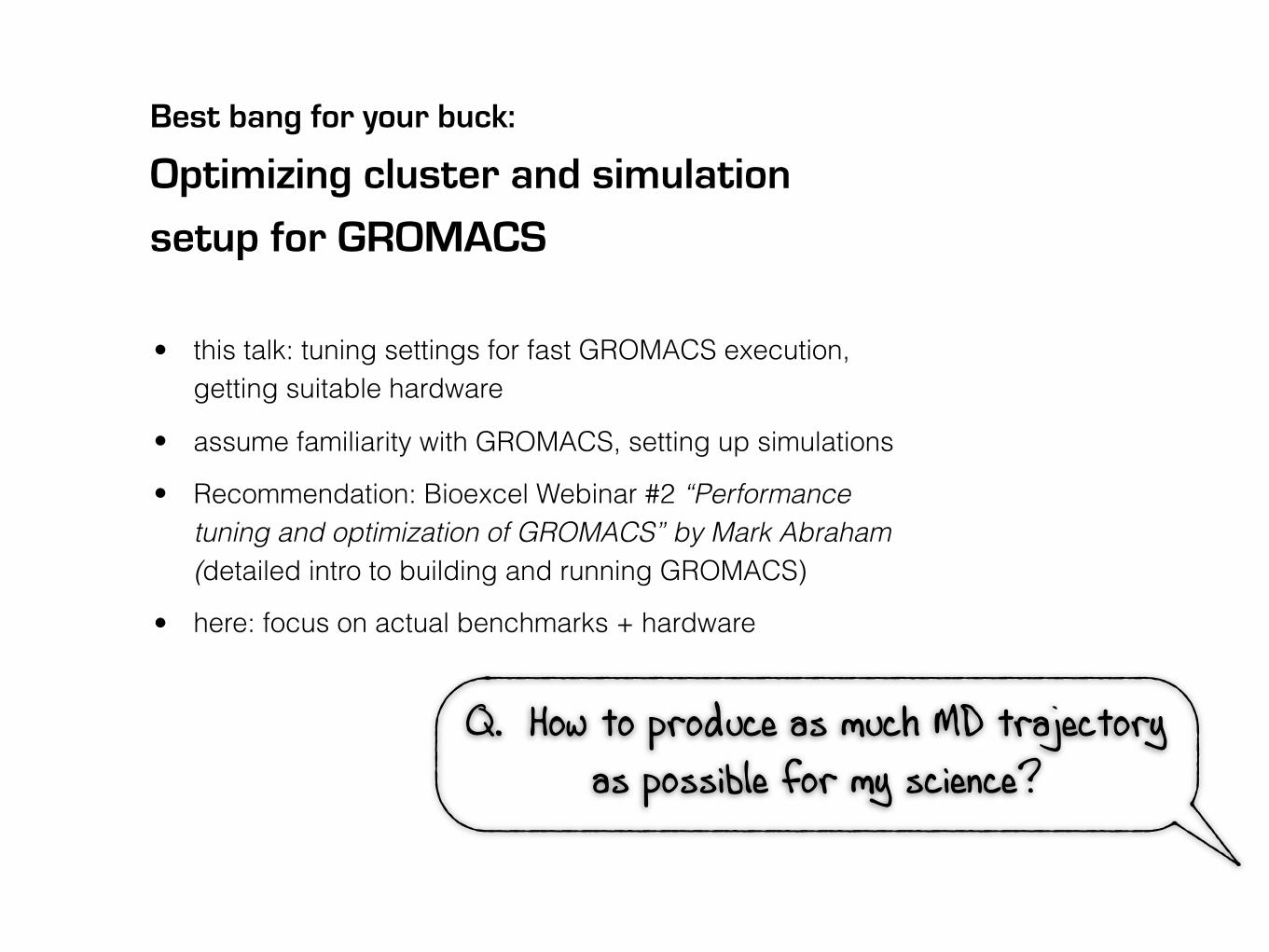
• this talk: tuning settings for fast GROMACS execution, getting suitable hardware

• assume familiarity with GROMACS, setting up simulations

• Recommendation: Bioexcel Webinar #2 “Performance tuning and optimization of GROMACS” by Mark Abraham (detailed intro to building and running GROMACS)

• here: focus on actual benchmarks + hardware

Q. How to produce as much MD trajectory as possible for my science?

I have access to compute resources

I want to buy a cluster

(core-h limited) (money limited)

Q. How to produce as much MD trajectory as possible for my science?

Q1. How can optimal performance be obtained?

Q2. What is the optimal hardware to run GROMACS on?

Q1.How can optimal GROMACS performance be obtained?

Before the simulation: The foundation of good performance

compilation, e.g. compiler, SIMD instructions, MPI library

system setup, e.g. virtual sites

When launching mdrun:main benefits come from optimizing the parallel run settings

reach a balanced computational load

keep communication overhead small

Coul. + vdW make up for most of the time step PME decomposes these into SR and LR contributions SR can be efficiently calculated in direct space LR can be efficiently calculated in reciprocal space recip. part needs FT of charge density

PME allows to shift work between real, SR (PP), and reciprocal, LR (PME), space parts (balance cutoff : grid spacing)

3D FFT

solve PME

3D inverse FFT

SR forces

spread charges

bonded forces

interpolate forces

3D FFT

solve PME

3D inverse FFT

SR forces

spread charges

bonded forces

interpolate forces

neighbor searching neighbor searching

update coordinates update coordinates

3D FFT

solve PME

3D inverse FFT

SR forces

spread charges

bonded forces

interpolate forces

neighbor searching

update coordinates

domain decomp. domain decomp. domain decomp.

initial xi, vi

neighbor searching

step?

Y

N

Recap: GROMACS serial time step

Coulomb & van der Waals

interactions

communication intense in parallel

more PME/CPU workmore PP/GPU work

direct space interactions decomposed into domains rMPI = nx x ny x nz

reciprocal space / LR PME use rMPI slabs

neighbor searching

step?

initial xi, vi

3D FFT

solve PME

3D inverse FFT

neighbor searching

SR forces

spread charges

bonded forces

interpolate forces

update coordinates

Y

Nr2r1r0 r3

...

r3r2r1 ...

3D FFT

solve PME

3D inverse FFT

SR forces

spread charges

bonded forces

interpolate forces

3D FFT

solve PME

3D inverse FFT

SR forces

spread charges

bonded forces

interpolate forces

neighbor searching neighbor searching

update coordinates update coordinates

3D FFT

solve PME

3D inverse FFT

SR forces

spread charges

bonded forces

interpolate forces

neighbor searching

update coordinates

domain decomp. domain decomp. domain decomp.

initial xi, vi

neighbor searching

step?

Y

N

OpenMP thread

MPI rankRecap: GROMACS parallel time step

r0 r1 r2

ü boundary layer communication

M all-to-all communication r2

during FFT grid transpose

PME calculation cost is O(N log N) with N atoms, but in parallel, PME communication becomes the bottleneck number of messages increases by r2, therefore also total latency

r3r2r1 ...r3

r2r1

...

M all-to-all r2 messages

Independent calculation of SR and LR forces

3D FFT

solve PME

3D inverse FFT

spread charges

interpolate forces

send forces

3D FFT

solve PME

3D inverse FFT

spread charges

interpolate forces

send forces

update coordinates update coordinates

domain decomp. domain decomp.

initial xi, vi

neighbor searching

step?

Y

N

send charges send charges receive charges receive charges

send positions send positions receive positions receive positions

Y

SR forces

bonded forces

neighbor searching

neighbor searching

step?N

SR forces

bonded forces

neighbor searching

neighbor searching

step?N

receive forcesreceive forces

neighbor searching

step?

YN

SR processes (direct space, PP) LR processes (Fourier space, PME)

offload LR electrostatics to a subset of MPI ranks typically 1/4 à reduces # of messages 16-fold

SR non-bonded forces can be offloaded to GPUs

neighbor searching neighbor searching

update coordinates update coordinates

domain decomp. domain decomp.

initial xi, vi

3D FFT

solve PME

3D inverse FFT

spread charges

interpolate forces

3D FFTsolve PME

3D inverse FFT

spread charges

interpolate forces

neighbor searching

step?

YN x, q

SR non-bondedforces

SR non-bondedforces

f, Ef, E

bonded forces bonded forces

x, q

1. Number of SR (PP) vs. LR (PME) processes is statically assigned

2. PME allows to shift work between real and reciprocal space parts!à fine-tune SR (PP) vs. LR (PME)(balance cutoff : grid spacing)

3. Balance direct space workload between SR domains

3D FFT

solve PME

3D inverse FFT

spread charges

interpolate forces

send forces

3D FFT

solve PME

3D inverse FFT

spread charges

interpolate forces

send forces

update coordinates update coordinates

domain decomp. domain decomp.

initial xi, vi

neighbor searching

step?

Y

N

send charges send charges receive charges receive charges

send positions send positions receive positions receive positions

Y

SR forces

bonded forces

neighbor searching

neighbor searching

step?N

SR forces

bonded forces

neighbor searching

neighbor searching

step?N

receive forcesreceive forces

neighbor searching

step?

YN

more PME/CPU workmore PP/GPU work

statically

assigned

continuously

once at start

of simulation

Automatic multi-level load balancing

Automatic multi-level load balancing

good news:on single nodes with a 1 CPU and opt. 1 GPU, GROMACS’ automatic settings often already give optimal performance (thread-MPI)

however, … on multi-GPU or multi-socket CPU nodes, or on a cluster of nodes, manual tuning will in most cases enhance performance

CPU

GPU

CPU CPU

GPU GPU

CPU

GPU

Tips & tricks for optimal GROMACS performance

If in doubt, make a benchmarkMost importantly:

testing different settings just takes few minutes

will directly uncover the optimal settings for your MD system on your hardware

most shown results obtained with these 2 systems:

3 Systematic performance evaluation

Benchmark input systems

Table 1: Specifications of the MD benchmark systems.

MD system membrane protein (MEM) ribosome (RIB)

# particles 81,743 2,136,412system size (nm) 10.8⇥10.2⇥9.6 31.2⇥31.2⇥31.2time step length (fs) 2 4cutoff radiia (nm) 1.0 1.0PME grid spacinga (nm) 0.120 0.135neighborlist update freq. CPU 10 25neighborlist update freq. GPU 40 40load balancing time steps 5,000 – 10,000 1,000 – 5,000benchmark time steps 5,000 1,000 – 5,000

aTable lists the initial values of Coulomb cutoff and PME grid spacing. These are adjusted for optimal load balanceat the beginning of a simulation.

For the performance evaluation on different hardware configurations we chose two represen-

tative biomolecular benchmark systems as summarized in Table 1. MEM is a membrane channel

protein embedded in a lipid bilayer surrounded by water and ions. With its size of ⇡ 80 k atoms

it serves as a prototypic example for a large class of setups used to study all kinds of membrane-

embedded proteins. RIB is a bacterial ribosome in water with ions9 and with more than two million

atoms an example of a rather large MD system that is usually run in parallel across several nodes.

Software environment

The benchmarks have been carried out with the most recent version of GROMACS 4.6 available

at the time of testing (see 5th column of Table 2). Results obtained with version 4.6 will in the

majority of cases hold for version 5.0 since the performance of CPU and GPU compute kernels

have not changed substantially. Moreover, as both compute kernel, threading and heterogeneous

parallelization design remains largely unchanged, performance characteristics and optimization

10

Both automatic load balancing mechanisms need time to reach the optimumReject the initial time steps from performance measurement withmdrun-resetstep2000mdrun-resethway

Getting useful performance numbers in benchmarksTip 1 of 10:

0 50 100 150 200

0.84

0.88

0.92

0.96

1

time steptim

e fo

r 10

step

s / t

0

8x1x1

4x4x1

8x2x1

8x2x2

4x4x4

8x4x4

domain decom-position grid

DDstep39loadimb.:force14.8%step80:timedwithpmegrid9696240,coulombcutoff1.200:2835.1M-cyclesstep160:timedwithpmegrid8484208,coulombcutoff1.311:2580.3M-cyclesstep240:timedwithpmegrid7272192,coulombcutoff1.529:3392.3M-cyclesstep320:timedwithpmegrid9696240,coulombcutoff1.200:2645.2M-cyclesstep400:timedwithpmegrid9696224,coulombcutoff1.212:2569.9M-cycles

…step1200:timedwithpmegrid9696208,coulombcutoff1.305:2669.8M-cyclesstep1280:timedwithpmegrid8484208,coulombcutoff1.311:2677.5M-cyclesstep1360:timedwithpmegrid8484200,coulombcutoff1.358:2770.5M-cyclesstep1440:timedwithpmegrid8080200,coulombcutoff1.376:2832.6M-cycles

optimalpmegrid9696224,coulombcutoff1.212DDstep4999volmin/aver0.777loadimb.:force0.6%DDstep9999volmin/aver0.769loadimb.:force1.1%

Both automatic load balancing mechanisms need time to reach the optimumReject the initial time steps from performance measurement withmdrun-resetstep2000mdrun-resethway

Getting useful performance numbers in benchmarks

md.log

Tip 1 of 10:

Determine optimal SR : LR process ratio (CPU nodes)

‣ GROMACS estimates SR : LR load, chooses near-optimal setting, based on cutoff + grid settings, but cannot know about network

‣ e.g.12 SR + 4 LR for 16 MPI processes

‣ gmxtune_pme tries settings around this value, e.g.14 : 213 : 312 : 4 *11 : 510 : 616 : 0 (no separate LR processes)

‣ For > 8 MPI ranks on CPU nodes (single or multiple nodes), usually separate PME nodes perform better

3D FFT

solve PME

3D inverse FFT

spread charges

interpolate forces

send forces

3D FFT

solve PME

3D inverse FFT

spread charges

interpolate forces

send forces

update coordinates update coordinates

domain decomp. domain decomp.

initial xi, vi

neighbor searching

step?

Y

N

send charges send charges receive charges receive charges

send positions send positions receive positions receive positions

Y

SR forces

bonded forces

neighbor searching

neighbor searching

step?N

SR forces

bonded forces

neighbor searching

neighbor searching

step?N

receive forcesreceive forces

neighbor searching

step?

YN

Tip 2 of 10:

Determine optimal SR : LR process ratio (CPU nodes)

‣ GROMACS estimates SR : LR load, chooses near-optimal setting, based on cutoff + grid settings, but cannot know about network

‣ e.g.12 SR + 4 LR for 16 MPI processes

‣ gmxtune_pme tries settings around this value, e.g.14 : 213 : 312 : 4 *11 : 510 : 616 : 0 (no separate LR processes)

‣ For > 8 MPI ranks on CPU nodes (single or multiple nodes), usually separate PME nodes perform better

Performance with and without tuning

8 16 24 32 480

5

10

15

20

25

perfo

rman

ce [n

s/da

y]

3.2

4.65.7

6.7

8.1 9.010.1 10.8

13.1 12.4

16.0

40processes

Tip 2 of 10:

+10-30%

DPPC, 2fs, 120k atoms, 8 core intel Harpertown nodes, IB

The optimal mix of threads & ranks (single node)Tip 3 of 10:

MPI + OpenMPà work can be distributed in various ways pure OpenMP performs well on single nodes, but does not scale well across sockets à on multi-socket nodes pure MPI is best OpenMP+MPI adds overhead

2x 8-core E5-2690 (Sandy Bridge), RNAse protein, solvated, 24k atoms, PME, 0.9 nm cutoffs (Fig. taken from S Pall, MJ Abraham, C Kutzner, B Hess, E Lindahl, EASC 2014, Springer, 2015)

0 2 4 6 8 10 12 14 160

10

20

30

40

50

60

70

80OpenMP

MPI

MPI+OpenMP (two ranks)

#cores

pe

rfo

rma

nce

(n

s/d

ay)

Figure 3: Comparison of single-node simulation performance using MPI,OpenMP, and combined MPI+OpenMP parallelization. The OpenMP multi-threading (blue) achieves the highest performance and near linear scaling upto 8 threads deteriorating only when threads on OpenMP regions need tocommunicate across the system bus. In contrast, the MPI-only paralel runs(red), requiring less communication scale well across sockets. CombiningMPI and OpenMP parallelization with two ranks and varying number ofthreads (green) results in worse performance due to the added overhead ofthe two parallizations.The simulations were carried out on a dual-socket node with 8-core Intel XeonE5-2690 (2.8 GHz Sandy Bridge). Input system: RNAse protein, solvated ina rectangular box, 24k atoms, PME electrostatics, 0.9 nm cut-o↵.

11

CPU CPUCPU

CPU CPU

GPU GPU

CPU

GPUWith GPUs it is beneficial to have few large domains offloading their data to the GPU à use pure OpenMP

Multi-socket GPU nodes à find optimum!

The optimal mix of threads & ranks (single node)Tip 3 of 10:

2x E5-2680v2 (2x 10 cores) processors with 4x GTX 980 GPUs

threadsranks

140

220

410

58

85104

202

140

220

410

58

85104

202

MEM RIB

no GPU

1 GPU

2 GPUs3 GPUs

4 GPUs

with DLBno DLB

CPU nodes:ü pure MPI

GPU nodes:ü several threads/rank

The optimal mix of threads & ranks (single node)Tip 3 of 10:

2x E5-2680v2 (2x 10 cores) processors with 4x GTX 980 GPUs

threadsranks

140

220

410

58

85104

202

140

220

410

58

85104

202

MEM RIB

no GPU

1 GPU

2 GPUs3 GPUs

4 GPUs

with DLBno DLB

+30 %

GPU nodes:ü several threads/rank

The optimal mix of threads & ranks (multi node)Tip 4 of 10:

2x E5-2680v2 “Ivy Bridge” processors / node with 2x K20X GPUs, FDR-14 IB (Hydra)

threads per rank

CPU CPU

GPU GPU

CPU CPU

CPU nodes:pure MPI or 2 OpenMP

threads per rank

With GPUs:2-5 threads per rank

Hyperthreading is beneficial at moderate parallelizationTip 5 of 10:

2x E5-2680v2 “Ivy Bridge” processors / node with 2x K20X GPUs, FDR-14 IB (Hydra)

40 threads per node (HT)

20 threads per nodeHT yields

+10 – 15% performance (single node) effect decreases with higher parallelization

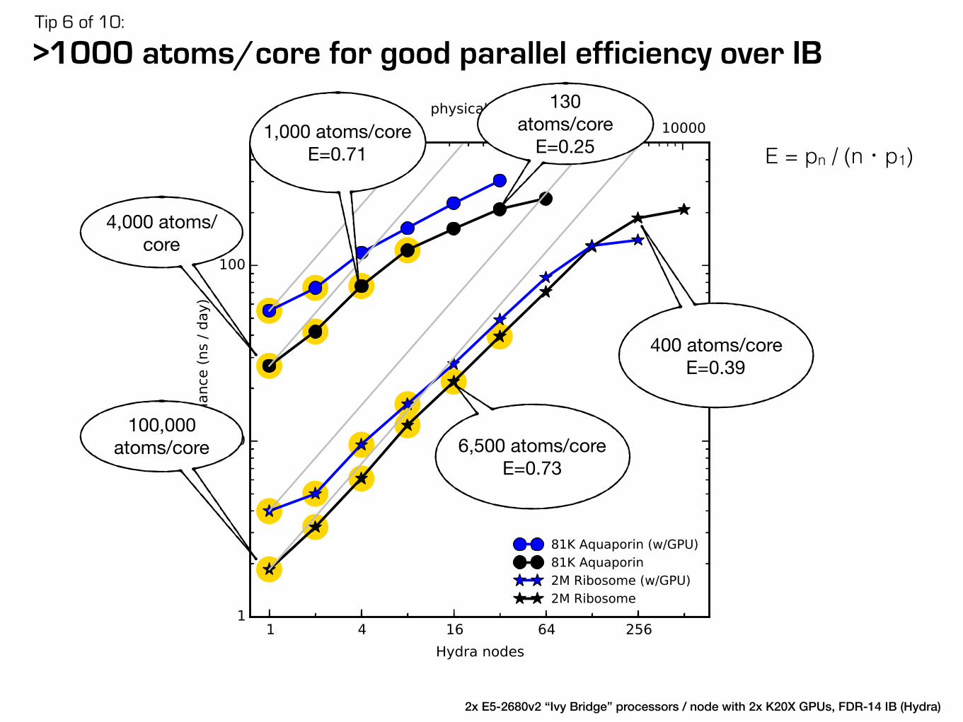
>1000 atoms/core for good parallel efficiency over IBTip 6 of 10:

2x E5-2680v2 “Ivy Bridge” processors / node with 2x K20X GPUs, FDR-14 IB (Hydra)

4,000 atoms/core

130 atoms/core

E=0.25

100,000 atoms/core

400 atoms/coreE=0.39

1,000 atoms/coreE=0.71

6,500 atoms/coreE=0.73

E = pn / (n・p1)

Separate LR PME nodes on GPU nodesTip 7 of 10:

usual approach would leave GPUs unused assigning half of the ranks to LR PME and interleave PME : PP nodes

SRdirectspace

SRdirectspace

SRdirectspace

LRPME LR PME

SR dir

LR PME

SR dir

LR PME

SR dir

LR PME

SR dir

x

mpirun-np128mdrun_mpi-npme64…

4 PP (SR) threads

6 PME (LR) threads

CPU0 CPU1 CPU0 CPU1

GPU0 GPU1 GPU0 GPU1

Infiniband Switch

node 3

node 1 node 2

p1 p3

p2 p4

SR ranks

LR ranks

mpirun-np128mdrun_mpi-npme64-ntomp4-ntomp_pme6-gpu_id01…

Separate LR PME nodes on GPU nodesTip 7 of 10:

assigning half of the ranks to LR PME, balance LR:SR load via threads

Impact of the compilerTip 8 of 10:

Table 3: GROMACS 4.6 single-node performance with thread-MPI (and CUDA 6.0) using differ-ent compiler versions on AMD and Intel hardware with and without GPUs. The last column showsthe speedup compared to GCC 4.4.7 calculated from the average of the speedups of the MEM andRIB benchmarks.

Hardware Compiler AQP (ns/d) RIB (ns/d) av. speedup (%)

AMD 6380 ⇥ 2 GCC 4.4.7 14 0.99 0GCC 4.7.0 15.6 1.11 11.8GCC 4.8.3 16 1.14 14.7ICC 13.1 12.5 0.96 �6.9

AMD 6380 ⇥ 2 GCC 4.4.7 40.5 3.04 0with 2⇥ GTX 980+ GCC 4.7.0 38.9 3.09 �1.2

GCC 4.8.3 40.2 3.14 1.3ICC 13.1 39.7 3.09 �0.2

Intel E5-2680v2 ⇥ 2 GCC 4.4.7 21.6 1.63 0GCC 4.8.3 26.8 1.86 19.1ICC 13.1 24.6 1.88 14.6ICC 14.0.2 25.2 1.81 13.9

Intel E5-2680v2 ⇥ 2 GCC 4.4.7 61.2 4.41 0with 2⇥ GTX 980+ GCC 4.8.3 62.3 4.69 4.1

ICC 13.1 60.3 4.78 3.5

GROMACS can be compiled in mixed precision (MP) or in double precision (DP). DP treats

all variables with double precision accuracy. MP treats almost all variables with DP accuracy with

the exception of the large arrays that contain the positions, forces, and velocities. All variables

requiring a high precision, like energies and the virial are always computed in double precision

accuracy, and it was shown that MP does not deteriorate energy conservation.1 Since MP produces

1.4 – 2⇥ more trajectory in the same compute time, it is in most cases preferable over DP.10

Therefore, we used MP for the benchmarking.

Table 3 shows the impact of the compiler version on simulation performance. From all tested

compilers, GCC 4.8 provides the fastest executable on both AMD and Intel platforms. On GPU

nodes, the difference between the fastest and slowest executable is at most 4%, but on nodes

without GPUs it is considerable and can reach up to 20%. Table 3 can also be used to normalize

benchmark results obtained with different compilers.

12

MEM

recent gcc’s >= 4.7 perform best can make a 25% difference

optimized performance!

Multi-simulations enhance throughputTip 9 of 10:

The GPU is typically idle for 15 – 40 % of a time step

Multi-simulation = running several replicas of a system mpirun-np4mdrun-multi4-gpu_id0011-sin.tpr

SR non bonded forces can interlock on GPUs so that aggregated performance is higher

+ benefits from higher efficiency at lower parallelization

idle

idle

CPUGPU

neighbor searching

update coordinates

domain decomp.

3D FFT

solve PME

3D inverse FFT

spread charges

interpolate forces

SR non-bondedforces

f, E

bonded forces

x, q

Multi-simulations enhance throughputTip 9 of 10:

2x E5-2680v2 node with 2x GTX980 GPUs 2x10 cores, 40 hyperthreads

x 1.4

x 1.5

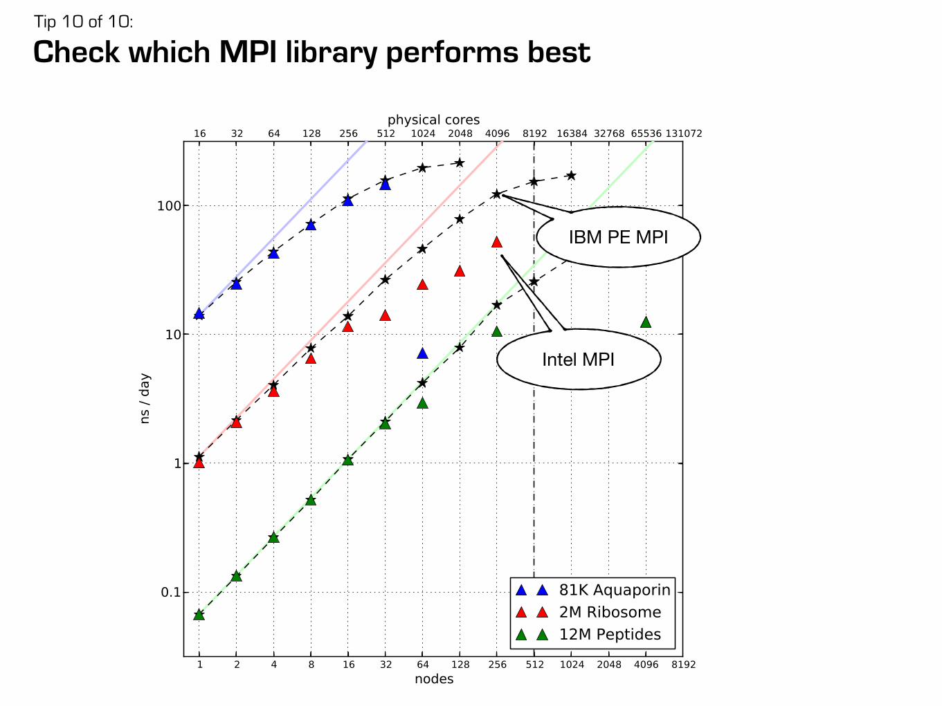
Check which MPI library performs bestTip 10 of 10:

IBM PE MPI

Intel MPI

typical trajectory gain

virtual sites x 2

multi simulations 50+ %

optimizing threads per rank on GPU nodes 20 – 40 %

Determine optimal # of PME nodes on CPU nodes using gmx tune_pme 10 – 30 %

Compiler up to 20 % on CPU nodes

hyper threading 10 – 15%

Q1 summarytr

ajec

tory

leng

th g

ain

‘optimal’ in terms of … ?

performance-to-price ratio achievable single-node performance parallel performance “time-to-solution” energy consumption “energy-to-solution” rack space requirements

with S Páll, M Fechner, A Esztermann, BL de Groot and H Grubmüller

Q2.

What is the ‘optimal’ hardware to run GROMACS on?

Our goal: Cost-efficient simulations. Maximize MD trajectory on a fixed budget

Method: Determine price + performance for >50 hardware configurations, 2 MD systems, 12 CPU types, 13 GPU types

determine ‘optimal’ performance per node type optimize threads x ranks optimize number of LR PME nodes use HT, where beneficial

with S Páll, M Fechner, A Esztermann, BL de Groot and H Grubmüller

Q2.

What is the ‘optimal’ hardware to run GROMACS on?

Table 4: Some GPU models that can be used by GROMACS. The upper part of the table lists HPC-class Tesla cards, below are the consumer-class GeForce GTX cards. For the GTX 980 GPUs, cardsby different manufacturers differing in clock rate were benchmarked, + and ‡ symbols are used todifferentiate between them.

NVIDIA architec- CUDA clock rate memory SP throughput ⇡ pricemodel ture cores (MHz) (GB) (Gflop/s) (e) (net)

Tesla K20Xa Kepler GK110 2,688 732 6 3,935 2,800Tesla K40a Kepler GK110 2,880 745 12 4,291 3,100

GTX 680 Kepler GK104 1,536 1,058 2 3,250 300GTX 770 Kepler GK104 1,536 1,110 2 3,410 320GTX 780 Kepler GK110 2,304 902 3 4,156 390GTX 780Ti Kepler GK110 2,880 928 3 5,345 520GTX Titan Kepler GK110 2,688 928 6 4,989 750GTX Titan X Maxwell GM200 3,072 1,002 12 6,156GTX 970 Maxwell GM204 1,664 1,050 4 3,494 250GTX 980 Maxwell GM204 2,048 1,126 4 4,612 430GTX 980+ Maxwell GM204 2,048 1,266 4 5,186 450GTX 980‡ Maxwell GM204 2,048 1,304 4 5,341 450

aSee Figure 4 for how performance varies with clock rate of the Tesla cards, all other benchmarks have been donewith the base clock rates reported in this table.

GPU acceleration

GROMACS 4.6 and later supports CUDA-compatible GPUs with compute capability 2.0 or higher.

Table 4 lists a selection of modern GPUs including some relevant technical information. The single

precision (SP) column shows the GPU’s maximum theoretical SP flop rate, calculated from the

base clock rate (as reported by NVIDIA’s deviceQuery program) times the number of cores times

two floating-point operations per core and cycle. GROMACS exclusively uses single precision

floating point (and integer) arithmetic on GPUs and can therefore only be used in mixed precision

mode with GPUs. Note that at comparable theoretical SP flop rate the Maxwell GM204 cards yield

a higher effective performance than Kepler generation cards due to better instruction scheduling

and reduced instruction latencies.

Since the GROMACS CUDA non-bonded kernels are by design strongly compute-bound,3

GPU main memory performance has little impact on their performance. Hence, peak performance

13

GPUs used in the test nodes 2014

MEM uses 50 MB of GPU RAM, RIB 225 MB

since v5.1 possible to use AMD GPUs via OpenCL, since v2016 full support with GPU sharing

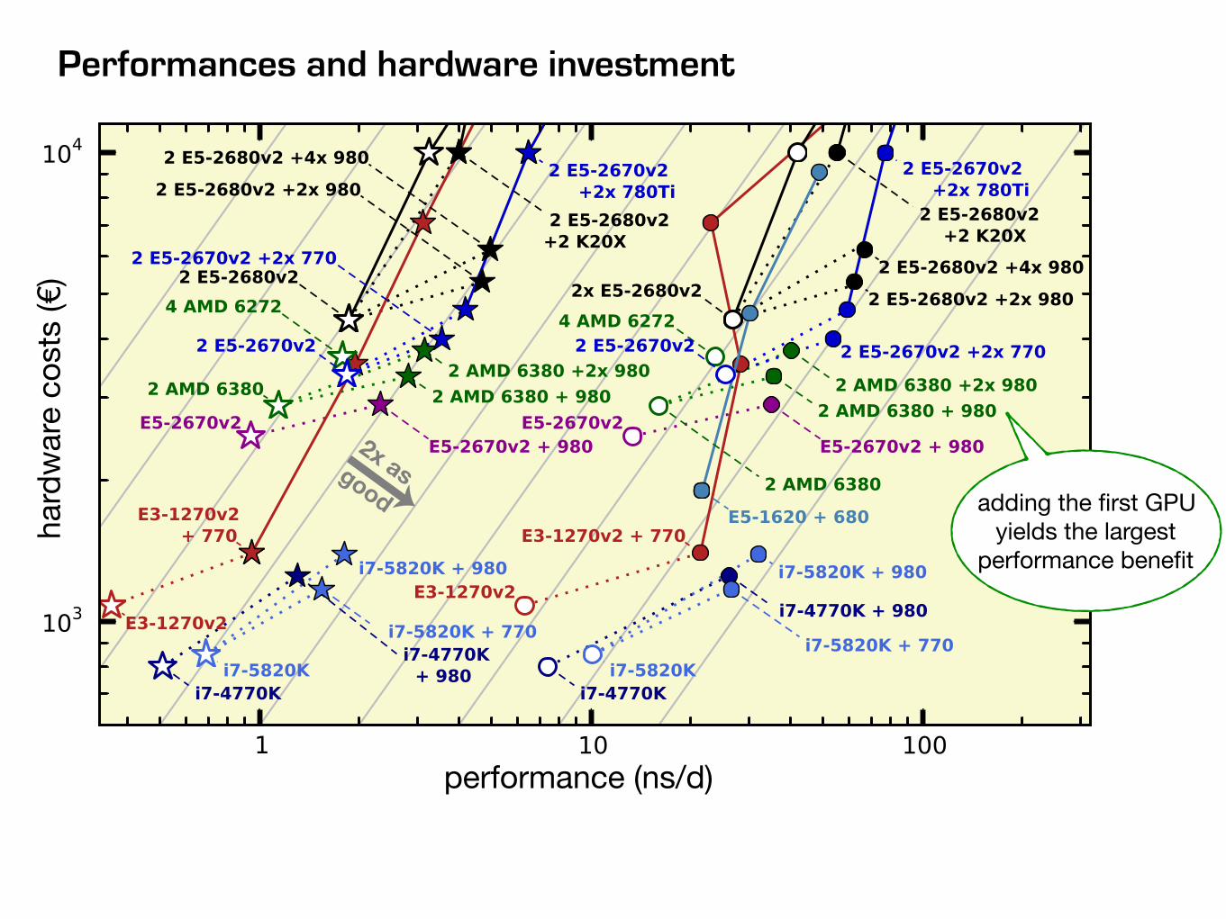
Performances and hardware investment

CPU nodes

nodes with consumer-class GPUs

u2equal

performance-to-price

nodes with Tesla GPUs

12 2

4

1

8

4

1

2

4

816

8

16

hard

ware

cos

ts (€

)

performance (ns/d)

2x as good

Performances and hardware investment

adding the first GPU yields the largest

performance benefit

Energy efficiency

Over cluster lifetime, energy costs become comparable to hardware costs assuming 5 yr of operation and 0.2 EUR / kWh (incl. cooling)

Table 1

Node ns/d microseconds power draw (W)

energy costs (Euro) node costs (Euro)

traj costs (Euro / microsecond)

just node just energy yield (ns per 1000 Euro)

2x E5-2670v2 1,38 2,5185 252 2207,52 3360 €2211 €1334 €877 €2211 452

2x E5-2670v2 + 780Ti 3,3 6,0225 519 4546,44 3880 €1399 €644 €755 €1399 715

2x E5-2670v2 + 2x 780Ti 3,87 7,06275 666 5834,16 4400 €1449 €623 €826 €1449 690

2x E5-2670v2 + 3x 780Ti 4,17 7,61025 933 8173,08 5430 €1787 €714 €1074 €1787 559

2x E5-2670v2 + 4x 780Ti 4,17 7,61025 960 8409,6 5950 €1887 €782 €1105 €1887 530

2x E5-2670v2 + 980 3,86 7,0445 408 3574,08 3780 €1044 €537 €507 €1044 958

2x E5-2670v2 + 2x 980 4,18 7,6285 552 4835,52 4200 €1184 €551 €634 €1184 844

2x E5-2670v2 + 3x 980 4,2 7,665 696 6096,96 5130 €1465 €669 €795 €1465 683

2x E5-2670v2 + 4x 980 4,2 7,665 840 7358,4 5550 €1684 €724 €960 €1684 594

2x E5-2680v2 1,86 3,3945 446 3906,96 4400 €2447 €1296 €1151 €2447 409

2x E5-2680v2 + 980 3,99 7,28175 622 5448,72 4850 €1414 €666 €748 €1414 707

2x E5-2680v2 + 2x 980 4,69 8,55925 799 6999,24 5300 €1437 €619 €818 €1437 696

2x E5-2680v2 + 3x 980 4,85 8,85125 926 8111,76 5750 €1566 €650 €916 €1566 639

2x E5-2680v2 + 4x 980 4,96 9,052 1092 9565,92 6200 €1742 €685 €1057 €1742 574

Trajectory production costs per microsecond

€0

€500

€1000

€1500

€2000

€2500

2x E

5-26

70v2

2x E

5-26

70v2

+ 7

80Ti

2x E

5-26

70v2

+ 2

x 78

0Ti

2x E

5-26

70v2

+ 3

x 78

0Ti

2x E

5-26

70v2

+ 4

x 78

0Ti

2x E

5-26

70v2

+ 9

80

2x E

5-26

70v2

+ 2

x 98

0

2x E

5-26

70v2

+ 3

x 98

0

2x E

5-26

70v2

+ 4

x 98

0

2x E

5-26

80v2

2x E

5-26

80v2

+ 9

80

2x E

5-26

80v2

+ 2

x 98

0

2x E

5-26

80v2

+ 3

x 98

0

2x E

5-26

80v2

+ 4

x 98

0

hardwareenergy

Trajectory costs per microsecond

2x E5-2680v2

2x E5-2680v2 + 1 GPU

2x E5-2680v2 + 2 GPUs

2x E5-2680v2 + 3 GPUs

2x E5-2680v2 + 4 GPUs

€0 €750 €1500 €2250 €3000

�1

energyhardware01234

GPUs

balanced CPU/GPU resources are

necessary!2x E5-2680v2 (2x 10 core) with GTX 980 GPUs, RIB benchmark

trajectory yield (ns / 1000 €)0 250 500 750 1000

2x E5-2670v2+1 GPU (GTX 780Ti)

2 GPUs3 GPUs

4 GPUs+1 GPU (GTX 980)

2 GPUs3 GPUs

4 GPUs

2x E5-2680v2+1 GPU (GTX 980)

2 GPUs3 GPUs

4 GPUs

Energy efficiency

Fixed budget trajectory yield taking into account energy + cooling (0.2 EUR / kWh) RIB

don’t add too many GPUs if you have

to pay for energy consumption

sam

e C

PU

sam

e G

PU

Q2 conclusions

adding a GPU yields 2-4x increased node performance

consumer class (GeForce) GPUs increase performance-to-price of a node more than twofold

more GPUs than CPU sockets yields diminishing returns

Highest energy efficiency for nodes with balanced CPU-GPU resources

Table 1

Node ns/d microseconds power draw (W)

energy costs (Euro) node costs (Euro)

traj costs (Euro / microsecond)

just node just energy yield (ns per 1000 Euro)

2x E5-2670v2 1,38 2,5185 252 2207,52 3360 €2211 €1334 €877 €2211 452

2x E5-2670v2 + 780Ti 3,3 6,0225 519 4546,44 3880 €1399 €644 €755 €1399 715

2x E5-2670v2 + 2x 780Ti 3,87 7,06275 666 5834,16 4400 €1449 €623 €826 €1449 690

2x E5-2670v2 + 3x 780Ti 4,17 7,61025 933 8173,08 5430 €1787 €714 €1074 €1787 559

2x E5-2670v2 + 4x 780Ti 4,17 7,61025 960 8409,6 5950 €1887 €782 €1105 €1887 530

2x E5-2670v2 + 980 3,86 7,0445 408 3574,08 3780 €1044 €537 €507 €1044 958

2x E5-2670v2 + 2x 980 4,18 7,6285 552 4835,52 4200 €1184 €551 €634 €1184 844

2x E5-2670v2 + 3x 980 4,2 7,665 696 6096,96 5130 €1465 €669 €795 €1465 683

2x E5-2670v2 + 4x 980 4,2 7,665 840 7358,4 5550 €1684 €724 €960 €1684 594

2x E5-2680v2 1,86 3,3945 446 3906,96 4400 €2447 €1296 €1151 €2447 409

2x E5-2680v2 + 980 3,99 7,28175 622 5448,72 4850 €1414 €666 €748 €1414 707

2x E5-2680v2 + 2x 980 4,69 8,55925 799 6999,24 5300 €1437 €619 €818 €1437 696

2x E5-2680v2 + 3x 980 4,85 8,85125 926 8111,76 5750 €1566 €650 €916 €1566 639

2x E5-2680v2 + 4x 980 4,96 9,052 1092 9565,92 6200 €1742 €685 €1057 €1742 574

Trajectory production costs per microsecond

€0

€500

€1000

€1500

€2000

€2500

2x E

5-26

70v2

2x E

5-26

70v2

+ 7

80Ti

2x E

5-26

70v2

+ 2

x 78

0Ti

2x E

5-26

70v2

+ 3

x 78

0Ti

2x E

5-26

70v2

+ 4

x 78

0Ti

2x E

5-26

70v2

+ 9

80

2x E

5-26

70v2

+ 2

x 98

0

2x E

5-26

70v2

+ 3

x 98

0

2x E

5-26

70v2

+ 4

x 98

0

2x E

5-26

80v2

2x E

5-26

80v2

+ 9

80

2x E

5-26

80v2

+ 2

x 98

0

2x E

5-26

80v2

+ 3

x 98

0

2x E

5-26

80v2

+ 4

x 98

0

hardwareenergy

Trajectory costs per microsecond

2x E5-2680v2

2x E5-2680v2 + 1 GPU

2x E5-2680v2 + 2 GPUs

2x E5-2680v2 + 3 GPUs

2x E5-2680v2 + 4 GPUs

€0 €750 €1500 €2250 €3000

�1

hardware energyGPUs01234

more details & tweaks in Best Bang for Your Buck: GPU Nodes for GROMACS Biomolecular Simulations (+supplement)C Kutzner, S Páll, M Fechner, A Esztermann, BL de Groot, H Grubmüller, J. Comput. Chem. 36, 1990–2008 (2015)

benchmark systems+helper scripts:www.mpibpc.mpg.de/grubmueller/gromacs

CPU nodes

nodes with consumer-class GPUs

u2equal

performance-to-price

nodes with Tesla GPUs

12 2

4

1

8

4

1

2

4

816

8

16

Fig. 8 performance

checklist

bioexcel.eu

Audience Q&A session

Please use the Questions function in GoToWebinar application

bioexcel.eu

Answerstotoday’squestionsathttp://ask.bioexcel.eu

Morewebinarscomingupsoon!http://bioexcel.eu/webinars

Followusonwww.bioexcel.eu/contact