GREENHOUSE GAS QUANTIFICATION DETERMINATION FOR THE SANTA BARBARA COUNTY ASSOCIATION OF GOVERNMENTS’

REGIONAL TRANSPORTATION PLAN/SUSTAINABLE COMMUNITIE S STRATEGY

STAFF REPORT

Date of Release: November 2013 Scheduled for Consideration: November 21, 2013

Electronic copies of this document can be found on ARB’s website at

http://www.arb.ca.gov/cc/sb375/sb375.htm.

This report has been reviewed by the staff of the California Air Resources Board and approved for publication. Approval does not signify that the contents necessarily reflect the views and policies of the Air Resources Board, nor does mention of trade names or commercial products constitute endorsement or recommendation for use.

TABLE OF CONTENTS

EXECUTIVE SUMMARY .................................................................................................. i

I. THE SANTA BARBARA REGION ............................................................................... 1

A. Description of the Region ................................................................................... 1

B. Transportation Planning in the Region ............................................................... 2

II. SBCAG’s RTP AND SCS DEVELOPMENT PROCESS ............................................. 2

A. Development and Adoption of the Growth Forecast ........................................... 2

B. Scenario Development ....................................................................................... 3

C. Public Input ........................................................................................................ 5

D. Selection of the Preferred Scenario ................................................................... 6

III. ARB STAFF REVIEW OF THE SBCAG SCS ........................................................... 7

A. Application of ARB Technical Methodology ....................................................... 7

B. Data Inputs and Assumptions ............................................................................ 7

1. Demographics and the SBCAG 2012 Regional Growth Forecast ................... 7

2. Current and Future Land Use Development Patterns ................................... 11

3. Transportation Network Inputs and Assumptions.......................................... 17

4. Travel Demand Model Inputs and Assumptions ........................................... 20

C. Modeling Tools ..................................................................................................... 21

1. Land Use Allocation Model (UPlan) .............................................................. 22

2. Travel Demand Model ................................................................................... 23

3. EMFAC Model............................................................................................... 32

D. Discussion of Model Sensitivity ............................................................................ 32

IV. PERFORMANCE INDICATORS ............................................................................. 33

A. Land Use – Residential Density ....................................................................... 33

B. Transportation - Passenger Vehicle Miles Traveled ......................................... 34

V. CONCLUSION ......................................................................................................... 34

VI. REFERENCES ........................................................................................................ 35

Appendix A: 2010 CTC RTP Guidelines ....................................................................... 37

Appendix B: Modeling Parameters for SCS Evaluation (Data Table) ........................... 40

LIST OF TABLES Table 1: Santa Barbara County Employment Forecast 2010-2040 ................................. 8 Table 2: Santa Barbara County Population Forecast 2010-2040 .................................... 9 Table 3: Santa Barbara County Household Forecast 2010-2040 .................................. 10 Table 4: RHNA Housing Need vs. UPlan Land Use Capacity – Total Units (Preferred Scenario) ....................................................................................................................... 10 Table 5: SBCAG Population, Households, and Employment by Jurisdiction ................. 11 Table 6: Percentage of Santa Barbara Land Area by General Plan Land Use Category for 2010 ......................................................................................................................... 13 Table 7: Distribution of Housing Units across Type and Average Density for 2020 and 2035 .............................................................................................................................. 17 Table 8: SBCAG 2010 Highway Network Lane Miles by Facility Type .......................... 18 Table 9: Reported SBCAG Lane Capacities and Free Flow Speeds ............................ 19 Table 10: 2010 SBCAG Transit Facility Lane Miles....................................................... 19 Table 11: Average Trip Rates per Person by Trip Purpose in 2010 .............................. 20 Table 12: Average Trip Length and Travel Time in 2010 .............................................. 21 Table 13: UPlan MCD Population Allocation Error Statistical Analysis.......................... 23 Table 14: Final Balanced Productions and Attractions for Base Year of 2010 .............. 26 Table 15: Survey and Model Trip Lengths and Travel Time for 2010 ............................ 28 Table 16: 2010 Mode Share ......................................................................................... 28 Table 17: Observed and Modeled Results for HBW and HBO Trips in 2010 ............... 29 Table 18: Shared Ride Occupancy Rates ..................................................................... 29 Table 19: Modeled 2010 VMT by Function Class .......................................................... 30 Table 20: Base Year Static Model Validation Results of the Daily Model ...................... 31 Table 21: Transit Frequency Sensitivity Test Results.................................................... 32

LIST OF FIGURES Figure 1: Santa Barbara County ...................................................................................... 1 Figure 2: SBCAG’s Three Phase Outreach Process ....................................................... 5 Figure 3: Santa Barbara Generalized Land Uses - 2010............................................... 14 Figure 4: Major Regions of Santa Barbara County ........................................................ 15 Figure 5: SBCAG’s Modeling Tools ............................................................................... 22 Figure 6: SBCAG’s Trip-Based Travel Demand Model ................................................. 24 Figure 7: Per Capita Passenger VMT and CO2 ............................................................ 34

i

EXECUTIVE SUMMARY The Sustainable Communities and Climate Protection Act of 2008 (SB 375) calls for the California Air Resources Board (ARB or Board) to accept or reject the determination of each Metropolitan Planning Organization (MPO) that their Sustainable Communities Strategy (SCS) would, if implemented, achieve the passenger vehicle greenhouse gas (GHG) emission reduction targets for 2020 and 2035, set by the Board in 2010. The Santa Barbara County Association of Governments (SBCAG) released the Public Review Draft of their Regional Transportation Plan (RTP), on April 26, 2013. The RTP includes a chapter that serves as the region’s SCS. It contains integrated land use and transportation strategies that will allow the Santa Barbara region to achieve the targets for reducing greenhouse gas emissions by 2035. This region, located on the south central coast, has a population of approximately 400,000 people and includes eight incorporated cities. The region has significant agricultural activity, a campus of the University of California, and Vandenberg Air Force Base. For the Santa Barbara region, the Board set passenger vehicle greenhouse gas reduction targets at a zero percent decrease for 2020 and at a zero percent decrease by 2035 based on the latest data available from SBCAG at that time. The SCS, adopted by the SBCAG Board in August 2013, affirms that the region will achieve reductions beyond the established targets by reducing greenhouse gas emissions by over 10 percent in 2020 and over 15 percent in 2035. On August 26, 2013, SBCAG transmitted the adopted SCS to ARB for review. Consistent with ARB’s July 2011 technical methodology for SCS evaluation, ARB staff prepared this technical report to support the Board’s action on SBCAG’s SCS. This report describes both the method ARB staff used to review the SBCAG SCS greenhouse gas quantification and the results of ARB staff’s technical evaluation. Specifically, staff reviewed how well the region’s travel demand modeling and related analyses provide for the quantification of GHG emission reductions associated with the SCS. This included reviewing data inputs, planning assumptions on future year land use, housing and transportation policies, and modeling results. This review affirms that SBCAG’s adopted SCS demonstrates that, if implemented, the region will achieve a 10.5 percent per capita passenger vehicle greenhouse gas reduction in 2020, and a 15.4 percent reduction in 2035, exceeding the established targets.

1

I. THE SANTA BARBARA REGION

A. Description of the Region

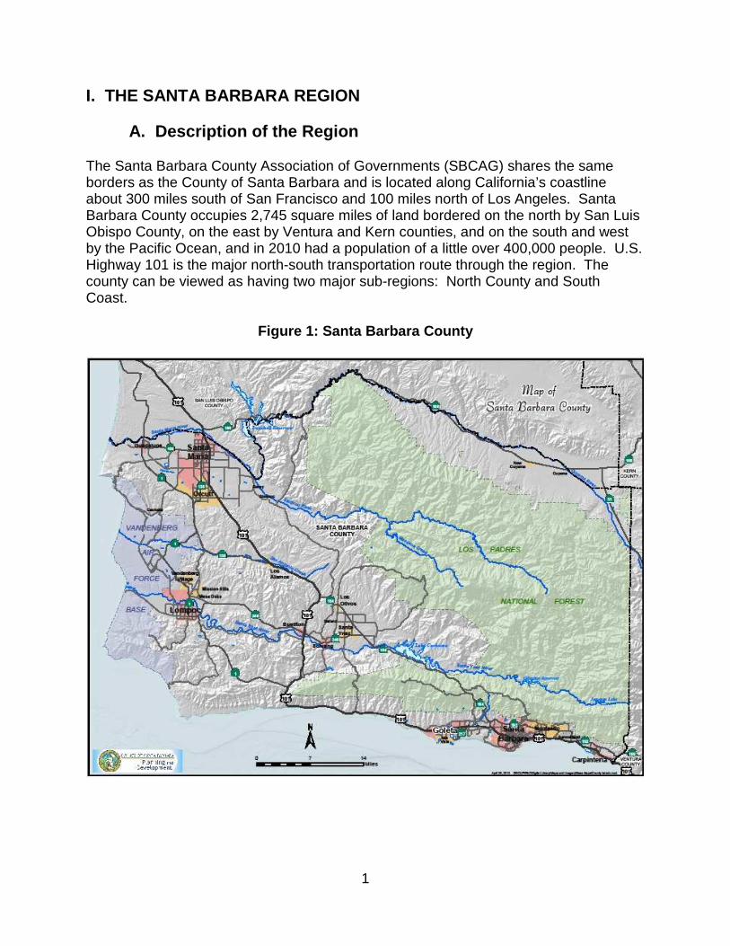
The Santa Barbara County Association of Governments (SBCAG) shares the same borders as the County of Santa Barbara and is located along California’s coastline about 300 miles south of San Francisco and 100 miles north of Los Angeles. Santa Barbara County occupies 2,745 square miles of land bordered on the north by San Luis Obispo County, on the east by Ventura and Kern counties, and on the south and west by the Pacific Ocean, and in 2010 had a population of a little over 400,000 people. U.S. Highway 101 is the major north-south transportation route through the region. The county can be viewed as having two major sub-regions: North County and South Coast.

Figure 1: Santa Barbara County

2

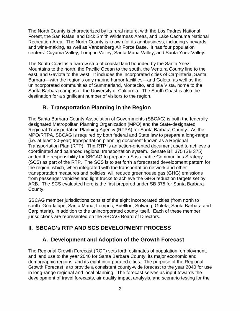
The North County is characterized by its rural nature, with the Los Padres National Forest, the San Rafael and Dick Smith Wilderness Areas, and Lake Cachuma National Recreation Area. The North County is known for its agribusiness, including vineyards and wine-making, as well as Vandenberg Air Force Base. It has four population centers: Cuyama Valley, Lompoc Valley, Santa Maria Valley, and Santa Ynez Valley.

The South Coast is a narrow strip of coastal land bounded by the Santa Ynez Mountains to the north, the Pacific Ocean to the south, the Ventura County line to the east, and Gaviota to the west. It includes the incorporated cities of Carpinteria, Santa Barbara—with the region’s only marine harbor facilities—and Goleta, as well as the unincorporated communities of Summerland, Montecito, and Isla Vista, home to the Santa Barbara campus of the University of California. The South Coast is also the destination for a significant number of visitors to the region.

B. Transportation Planning in the Region

The Santa Barbara County Association of Governments (SBCAG) is both the federally designated Metropolitan Planning Organization (MPO) and the State-designated Regional Transportation Planning Agency (RTPA) for Santa Barbara County. As the MPO/RTPA, SBCAG is required by both federal and State law to prepare a long-range (i.e. at least 20-year) transportation planning document known as a Regional Transportation Plan (RTP). The RTP is an action-oriented document used to achieve a coordinated and balanced regional transportation system. Senate Bill 375 (SB 375) added the responsibility for SBCAG to prepare a Sustainable Communities Strategy (SCS) as part of the RTP. The SCS is to set forth a forecasted development pattern for the region, which, when integrated with the transportation network and other transportation measures and policies, will reduce greenhouse gas (GHG) emissions from passenger vehicles and light trucks to achieve the GHG reduction targets set by ARB. The SCS evaluated here is the first prepared under SB 375 for Santa Barbara County.

SBCAG member jurisdictions consist of the eight incorporated cities (from north to south: Guadalupe, Santa Maria, Lompoc, Buellton, Solvang, Goleta, Santa Barbara and Carpinteria), in addition to the unincorporated county itself. Each of these member jurisdictions are represented on the SBCAG Board of Directors.

II. SBCAG’s RTP AND SCS DEVELOPMENT PROCESS

A. Development and Adoption of the Growth Forecast The Regional Growth Forecast (RGF) sets forth estimates of population, employment, and land use to the year 2040 for Santa Barbara County, its major economic and demographic regions, and its eight incorporated cities. The purpose of the Regional Growth Forecast is to provide a consistent county-wide forecast to the year 2040 for use in long-range regional and local planning. The forecast serves as input towards the development of travel forecasts, air quality impact analysis, and scenario testing for the

3

RTP/SCS. SBCAG has utilized land use and travel models to assess the impacts of these changes in population, as well as employment, and to forecast future travel patterns. The SBCAG Board of Directors adopted the previous Regional Growth Forecasts in 2007. The forecast is updated as new data or policy changes occur to ensure that it provides the most accurate assessment of future growth. The current 2012 RGF integrates updated data from recent housing element and general plan updates and the 2010 Census. The SBCAG region-wide employment projections were based on a top-down approach using national and State projections developed in 2011. The forecast is based on a two-step growth forecast methodology, involving a county-wide, top-down employment and population forecast in the first step and the allocation of both employment and population forecasts to the sub-regional level in the second step, using a bottom-up method considering local general plan land use.

B. Scenario Development Development of the Sustainable Communities Strategy involved the study of eight separate land use and transportation scenarios, each analyzing different combinations of land use and transportation variables. SBCAG reports that all scenarios applied the same region-wide population, employment and housing projections from the 2012 SBCAG Regional Growth Forecast. However, sub-regional distribution of forecast population growth varies by scenario consistent with allowable land uses, residential land use capacity, and policy assumptions.

1. Future Baseline. The future baseline scenario is essentially a “business as usual” scenario, which assumes the following: existing, adopted general plan land uses, and construction of programmed and planned RTP projects, including new limited bus transit service. The future baseline scenario was the starting point for delineation of other alternative scenarios which were considered in the RTP/SCS and was the primary basis for comparison of other scenarios.

2. No Project. This scenario is identical to the future baseline, but omits any new

RTP projects, except already programmed projects. 3. Transit-Oriented Development (TOD)/Infill. By selectively increasing residential

and commercial land use capacity within existing transit corridors, this scenario tests land use changes that shift a greater share of future growth to these corridors. Land use change assumptions were made based on location of existing transit routes and service. Assumed changes in land use capacity reflect local planning discussions about possible future land use and general plan and community plan updates under discussion at the local level. Future growth

4

distribution directly addresses jobs/housing balance issues by emphasizing job growth in the North County and housing growth in the South County.

4. Urban Area Expansion. Growth occurs in this scenario on land made available at

the urban fringe in a low-density pattern. In lieu of new infill areas, development occurs on land contiguous with and adjacent to the urban edge. Delineation of this scenario was based on local agency input, with reference in many instances to land use changes proposed in the past.

5. Blended Infill/Expansion. This scenario is a hybrid scenario which combines the

land use elements of both the TOD/Infill and Urban Area Expansion scenarios (Scenarios 3 and 4). Growth distribution occurs based on increased residential and commercial land use capacity both in core urban areas along transit lines as in Scenario 3 and at the urban edge as in Scenario 4.

6. North County-weighted Jobs, South County-weighted Housing Emphasis. This

scenario begins with existing, adopted land uses, but applies model weightings to make specific growth distribution assumptions emphasizing job growth in the North County and housing growth in the South County, within existing available land use capacity. Unlike the future baseline scenario, it does not continue past growth trends. Unlike Scenario 3, growth is distributed consistent with land uses designations in adopted general plans and the distribution places no explicit emphasis on TOD or infill. Infill occurs, but only to the degree that locally adopted land use designations allow.

7. TOD/Infill + Enhanced Transit. Based on the land use pattern from the TOD/Infill

scenario, this scenario enhances transit by maximizing alternative mode projects using available flexible funding sources for transit and assumes possible new funding sources for transit. In general, enhancements include doubling bus frequencies along existing local and intercity transit routes during peak periods and selectively adding new routes.

8. Historic Commute Trend Continued. A variation on the future baseline Scenario

1, this scenario changes the in-commuting assumption so that net in-commuting doubles over twenty years, continuing the historic growth of in-commuting.

SBCAG staff compared the performance of modeled scenarios for each of three target years (2020, 2035 and 2040) with the base year (2005) and the future baseline year (2040). Scenarios had to meet the SB 375 greenhouse gas (GHG) emission targets set for SBCAG in order to be viable candidates for consideration as the preferred RTP/SCS scenario. Four of the scenarios (Scenarios 3, 5, 6 and 7) met this initial test (i.e., they met the SBCAG targets of zero net growth in per capita emissions from passenger vehicles in for 2020 and 2035) and were therefore eligible for consideration as the preferred scenario in the RTP/SCS.

5

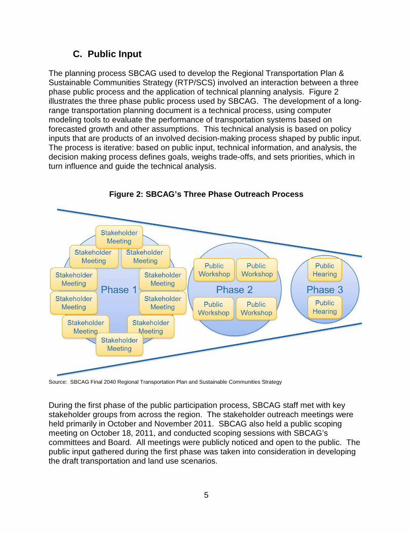
C. Public Input The planning process SBCAG used to develop the Regional Transportation Plan & Sustainable Communities Strategy (RTP/SCS) involved an interaction between a three phase public process and the application of technical planning analysis. Figure 2 illustrates the three phase public process used by SBCAG. The development of a long-range transportation planning document is a technical process, using computer modeling tools to evaluate the performance of transportation systems based on forecasted growth and other assumptions. This technical analysis is based on policy inputs that are products of an involved decision-making process shaped by public input. The process is iterative: based on public input, technical information, and analysis, the decision making process defines goals, weighs trade-offs, and sets priorities, which in turn influence and guide the technical analysis.

Figure 2: SBCAG’s Three Phase Outreach Process

Source: SBCAG Final 2040 Regional Transportation Plan and Sustainable Communities Strategy

During the first phase of the public participation process, SBCAG staff met with key stakeholder groups from across the region. The stakeholder outreach meetings were held primarily in October and November 2011. SBCAG also held a public scoping meeting on October 18, 2011, and conducted scoping sessions with SBCAG’s committees and Board. All meetings were publicly noticed and open to the public. The public input gathered during the first phase was taken into consideration in developing the draft transportation and land use scenarios.

6

In the second phase scoping meetings, SBCAG staff described the planning process, explained the significance of Senate Bill 375 (SB 375), and outlined the general planning goal (i.e., how to meet the GHG emission targets, accommodate future growth and meet the region’s transportation needs). SBCAG explained what types of land use and transportation methods the region could use to meet the targets and provided example scenarios, which consisted of visions of transportation infrastructure and operations, land use development patterns, and transportation measures and policies extending out for 20 years and beyond. SBCAG sought input into the range of land use and transportation alternative scenarios as well as other kinds of information the RTP/SCS should consider. During the third phase of the public participation process, SBCAG publically noticed and held a public comment meeting on the Draft RTP/SCS and Draft Environmental Impact Report (EIR). SBCAG also published notice of and held two public hearings on the Draft RTP/SCS and Draft EIR during regular meetings of the SBCAG Board of Directors. During the public hearings and the public review period, participants had the opportunity to review and comment on the preferred alternative, which was selected based on input received during the first two phases of the public participation process. The draft RTP/SCS was released for a 55 day public comment period on April 26, 2013, and the Draft EIR was released for a 45-day public comment period on May 28, 2013.

D. Selection of the Preferred Scenario The scenarios, discussed in Section B above, were developed with input from policy makers, stakeholders, and the general public and were analyzed to determine how each scenario performed across the range of SBCAG performance measures, including GHG emissions. Following an extensive public process, involving multiple workshops and hearings, analysis, and comparison of alternative scenarios, together with public input, the SBCAG Board selected the preferred scenario. The preferred scenario was selected from the scenario options based on the performance of each scenario as quantified by the adopted performance measures tied to the overall goals of the SCS. The preferred scenario selected by SBCAG, which forms the basis for the SCS evaluated here, is a combination of scenarios 3 and 7. It consists of three core inter-related components: a land use plan, including residential densities and building intensities sufficient to accommodate projected population, household and employment growth; a multi-modal transportation network to serve the region’s transportation needs; and a “regional green print” cataloguing open space, habitat, farmland, and other resource areas which can serve as constraints to urban development. The SBCAG preferred scenario is designed to selectively increase residential and commercial land use capacity within existing transit corridors, shifting a greater share of future growth to these corridors.

7

III. ARB STAFF REVIEW OF THE SBCAG SCS

A. Application of ARB Technical Methodology The review of SBCAG’s SCS focuses on the technical aspects of regional modeling that underlie the quantification of GHG reductions. This review examines the SBCAG model inputs and assumptions, modeling tools, application of the model, and modeling results, following the general method described in ARB’s July 2011 document entitled “Description of Methodology for ARB Staff Review of Greenhouse Gas Reductions from Sustainable Communities Strategies Pursuant to SB 375.” ARB staff tailored the general methodology to address the unique characteristics of the Santa Barbara County region and its transportation modeling approach. ARB staff evaluated how the SBCAG models operate and perform in estimating travel demand, and how well they provide for quantification of GHG emissions reductions associated with the SCS. In evaluating whether the SBCAG model is reasonably sensitive for these purposes, ARB staff examined how well SBCAG’s travel demand model responded to specific changes in input values, as well as how accurately it replicated observed results. To help answer these and other questions, ARB staff used publicly available information in the SBCAG SCS, including RTP technical appendices, the Draft Environment Impact Report (EIR), and the travel model description and validation reports. In order to assess the technical soundness and general accuracy of the SBCAG GHG quantification, three central components of the SBCAG GHG analyses were evaluated: data inputs and assumptions, modeling tools, model sensitivity and performance indicators. The evaluation of these four components is described below.

B. Data Inputs and Assumptions

1. Demographics and the SBCAG 2012 Regional Growth Forecast

Demographic data and demographic forecasts are critical inputs to the development of the RTP/SCS, and they describe a number of key characteristics used in travel demand models. Demographic data form the vision of how many people will live in the region, how many jobs the region will have, and the anticipated number of households. The SBCAG 2012 Regional Growth Forecast (the 2012 RGF) is based on a two-step growth forecast methodology. The first step uses a county-wide, top-down employment and population forecast. Regional employment is predicted from an estimated regional share of California jobs using statewide employment and national trends developed in 2011. The population forecast is based on the ratio of population to jobs predicted by the employment forecast, while considering assumptions that increase the number of workers commuting into the region from outside for work, and the existence of an excess of workers in the labor force due to current high unemployment. The household forecast is based on the application of household headship rates (i.e., the rates at which new households are formed) to the population forecast. The second step allocates both

8

employment and population forecasts to the sub-regional level. This allocation uses a bottom-up method which considers local general plan land uses.

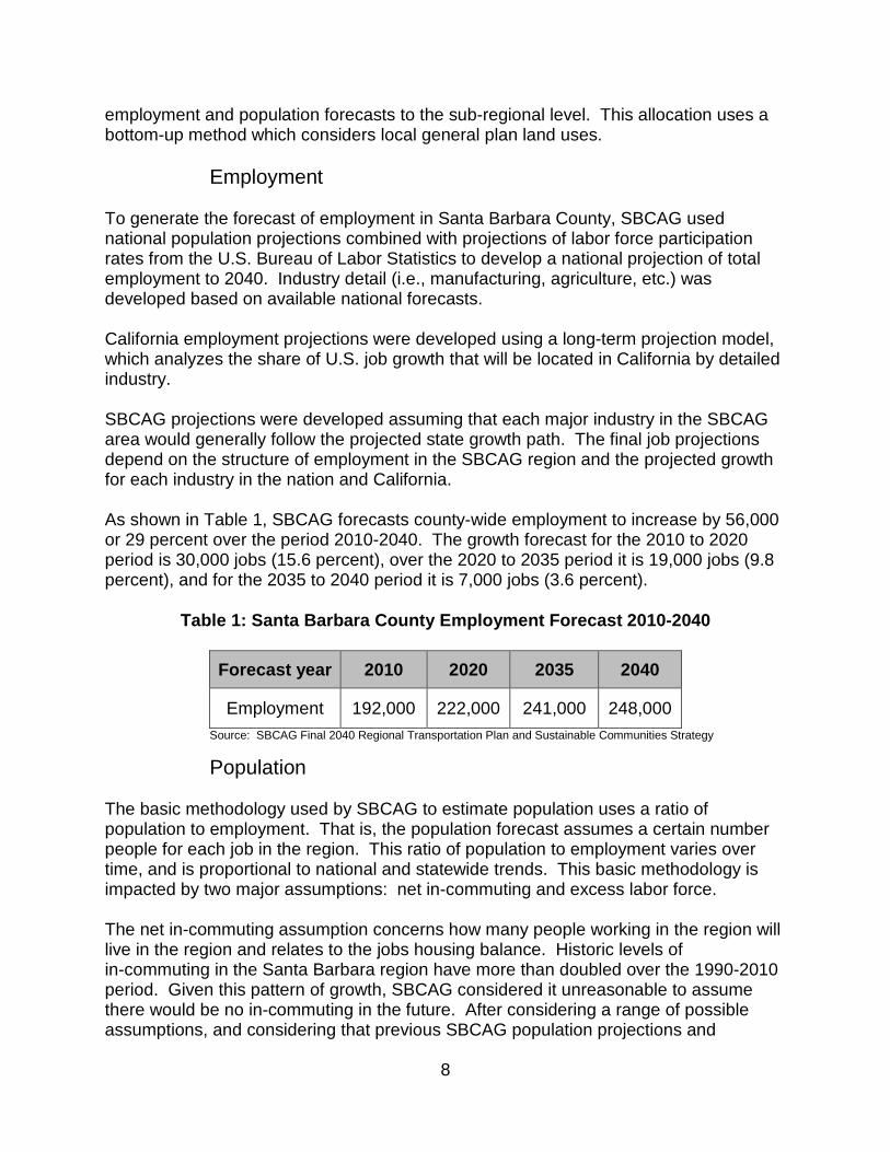
Employment To generate the forecast of employment in Santa Barbara County, SBCAG used national population projections combined with projections of labor force participation rates from the U.S. Bureau of Labor Statistics to develop a national projection of total employment to 2040. Industry detail (i.e., manufacturing, agriculture, etc.) was developed based on available national forecasts. California employment projections were developed using a long-term projection model, which analyzes the share of U.S. job growth that will be located in California by detailed industry. SBCAG projections were developed assuming that each major industry in the SBCAG area would generally follow the projected state growth path. The final job projections depend on the structure of employment in the SBCAG region and the projected growth for each industry in the nation and California. As shown in Table 1, SBCAG forecasts county-wide employment to increase by 56,000 or 29 percent over the period 2010-2040. The growth forecast for the 2010 to 2020 period is 30,000 jobs (15.6 percent), over the 2020 to 2035 period it is 19,000 jobs (9.8 percent), and for the 2035 to 2040 period it is 7,000 jobs (3.6 percent).

Table 1: Santa Barbara County Employment Forecast 2 010-2040

Forecast year 2010 2020 2035 2040

Employment 192,000 222,000 241,000 248,000 Source: SBCAG Final 2040 Regional Transportation Plan and Sustainable Communities Strategy

Population The basic methodology used by SBCAG to estimate population uses a ratio of population to employment. That is, the population forecast assumes a certain number people for each job in the region. This ratio of population to employment varies over time, and is proportional to national and statewide trends. This basic methodology is impacted by two major assumptions: net in-commuting and excess labor force. The net in-commuting assumption concerns how many people working in the region will live in the region and relates to the jobs housing balance. Historic levels of in-commuting in the Santa Barbara region have more than doubled over the 1990-2010 period. Given this pattern of growth, SBCAG considered it unreasonable to assume there would be no in-commuting in the future. After considering a range of possible assumptions, and considering that previous SBCAG population projections and

9

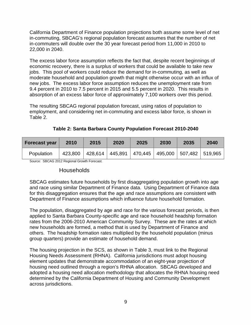
California Department of Finance population projections both assume some level of net in-commuting, SBCAG’s regional population forecast assumes that the number of net in-commuters will double over the 30 year forecast period from 11,000 in 2010 to 22,000 in 2040. The excess labor force assumption reflects the fact that, despite recent beginnings of economic recovery, there is a surplus of workers that could be available to take new jobs. This pool of workers could reduce the demand for in-commuting, as well as moderate household and population growth that might otherwise occur with an influx of new jobs. The excess labor force assumption reduces the unemployment rate from 9.4 percent in 2010 to 7.5 percent in 2015 and 5.5 percent in 2020. This results in absorption of an excess labor force of approximately 7,100 workers over this period. The resulting SBCAG regional population forecast, using ratios of population to employment, and considering net in-commuting and excess labor force, is shown in Table 2.

Table 2: Santa Barbara County Population Forecast 2 010-2040

Forecast year 2010 2015 2020 2025 2030 2035 2040

Population 423,800 428,614 445,891 470,445 495,000 507,482 519,965 Source: SBCAG 2012 Regional Growth Forecast.

Households SBCAG estimates future households by first disaggregating population growth into age and race using similar Department of Finance data. Using Department of Finance data for this disaggregation ensures that the age and race assumptions are consistent with Department of Finance assumptions which influence future household formation. The population, disaggregated by age and race for the various forecast periods, is then applied to Santa Barbara County-specific age and race household headship formation rates from the 2006-2010 American Community Survey. These are the rates at which new households are formed, a method that is used by Department of Finance and others. The headship formation rates multiplied by the household population (minus group quarters) provide an estimate of household demand. The housing projection in the SCS, as shown in Table 3, must link to the Regional Housing Needs Assessment (RHNA). California jurisdictions must adopt housing element updates that demonstrate accommodation of an eight-year projection of housing need outlined through a region’s RHNA allocation. SBCAG developed and adopted a housing need allocation methodology that allocates the RHNA housing need determined by the California Department of Housing and Community Development across jurisdictions.

10

Table 3: Santa Barbara County Household Forecast 20 10-2040

Forecast year 2010 2015 2020 2025 2030 2035 2040

Households 142,100 143,500 149,000 159,600 170,200 177,400 183,600 Source: SBCAG 2012 Regional Growth Forecast.

Table 4 shows the relationship between modeled land use capacities from the SBCAG UPlan model for the preferred scenario and identified housing need by jurisdiction, including very low and low income categories. The table shows that there is enough modeled residential housing capacity by jurisdiction to accommodate the eight-year housing need of 11,030 units projected for the 2014-2022 period for the SBCAG region by the California Department of Housing and Community Development. It should be noted that adopted general plans, not the RTP/SCS, determine allowable land uses and actual available land use capacity in each jurisdiction.

Table 4: RHNA Housing Need vs. UPlan Land Use Capac ity – Total Units (Preferred Scenario)

Source: SBCAG Final 2040 Regional Transportation Plan and Sustainable Communities Strategy

Region Jurisdiction

UPlan Land Use Capacity

RHNA Housing Need

UPlan Capacity Minus RHNA Need

South County Carpinteria 492 163 329

Santa Barbara 13,550 4,099 9,451 Goleta 6,550 979 5,571

Unincorporated 7,342 501 6,841 Total South County 27,933 5,743 22,190 Santa Ynez Valley

Solvang 1,092 175 917 Buellton 1,293 275 1,018

Unincorporated 446 7 439 Total Santa Ynez Valley 2,831 457 2,374 Lompoc Valley

Lompoc 10,965 525 10,440 Unincorporated 1,280 50 1,230

Total Lompoc Valley 12,244 575 11,669 Santa Maria Valley

Santa Maria 15,092 4,102 10,990 Guadalupe 2,347 50 2,297

Unincorporated 2,996 103 2,893 Total Santa Maria Valley 20,435 4,255 16,180 County Totals

Unincorporated 12,063 661 11,402 County -wide 63,444 11,030 52,414

11

Allocation of Population, Housing and Employment in the County

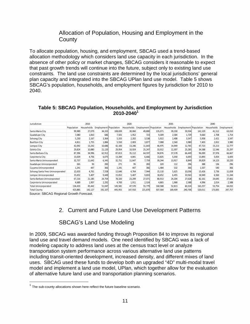
To allocate population, housing, and employment, SBCAG used a trend-based allocation methodology which considers land use capacity in each jurisdiction. In the absence of other policy or market changes, SBCAG considers it reasonable to expect that past growth trends will continue into the future, subject only to existing land use constraints. The land use constraints are determined by the local jurisdictions’ general plan capacity and integrated into the SBCAG UPlan land use model. Table 5 shows SBCAG’s population, households, and employment figures by jurisdiction for 2010 to 2040.

Table 5: SBCAG Population, Households, and Employme nt by Jurisdiction 2010-20401

Source: SBCAG Regional Growth Forecast.

2. Current and Future Land Use Development Patterns

SBCAG’s Land Use Modeling In 2009, SBCAG was awarded funding through Proposition 84 to improve its regional land use and travel demand models. One need identified by SBCAG was a lack of modeling capacity to address land uses at the census tract level or analyze transportation system performance across various alternative land use patterns including transit-oriented development, increased density, and different mixes of land uses. SBCAG used these funds to develop both an upgraded “4D” multi-modal travel model and implement a land use model, UPlan, which together allow for the evaluation of alternative future land use and transportation planning scenarios.

1 The sub-county allocations shown here reflect the future baseline scenario.

Jurisdiction

Population Households Employment Population Households Employment Population Households Employment Population Households Employment

Santa Maria City 99,989 27,079 34,333 108,839 30,060 49,800 135,071 39,230 59,934 141,529 41,512 63,010

Guadalupe City 7,080 1,810 686 7,501 1,952 723 9,309 2,584 1,729 9,660 2,708 1,754

Solvang City 5,230 2,167 3,364 5,333 2,202 3,538 5,922 2,408 3,547 5,958 2,421 3,547

Buellton City 4,811 1,755 1,884 5,550 2,003 3,877 7,088 2,540 3,980 7,403 2,652 3,980

Lompoc City 42,092 13,242 10,686 42,100 13,246 11,643 46,975 14,949 12,765 47,723 15,213 12,777

Goleta City 29,824 10,880 21,120 29,954 10,924 25,247 33,912 12,307 25,285 34,588 12,546 25,297

Santa Barbara City 87,396 34,996 62,912 87,813 35,112 64,597 94,876 37,578 66,449 96,000 37,976 66,667

Carpinteria City 13,029 4,756 6,075 13,284 4,841 6,666 13,825 5,030 6,693 13,893 5,054 6,693

Santa Maria Unincorporated 32,737 11,642 6,345 32,751 11,647 7,759 39,244 13,917 8,849 39,829 14,123 10,220

Guadalupe Unincorporated 265 93 283 271 95 283 320 112 296 388 136 296

Cuyama Unincorporated 1,241 447 366 1,241 447 366 1,484 532 366 1,507 540 366

Solvang-Santa Ynez Unincorporated 12,633 4,761 7,558 12,646 4,764 7,944 15,110 5,625 10,036 15,426 5,736 11,658

Lompoc Unincorporated 15,652 5,407 9,449 15,652 5,407 9,833 18,652 6,455 10,563 18,949 6,560 11,244

Santa Barbara Unincorporated 67,216 21,185 24,754 78,320 23,299 27,071 80,913 24,204 27,628 82,161 24,645 27,661

Carpinteria Unincorporated 4,689 1,907 2,292 4,700 1,911 2,524 4,865 1,968 2,588 4,996 2,014 2,588

Total Unincorporated 134,433 45,442 51,047 145,581 47,570 55,779 160,588 52,813 60,324 163,257 53,754 64,032

Total County 423,885 142,127 192,107 445,955 147,910 221,870 507,564 169,439 240,706 520,011 173,835 247,757

2010 2020 2035 2040

12

UPlan is a computer software application that was developed at the Information Center for the Environment at the University of California, Davis, which allows users to project future land use patterns. Users can also overlay environmental data with the urban footprint to identify potential conflicts. UPlan was designed for use in California and has been widely applied in land use and environmental planning. The UPlan modeling process starts by replicating existing allowable land use designations across all SBCAG member jurisdictions. For the 2010 base year, allowable land uses were designed to replicate the existing land use designations allowed by each of the general plan land use and housing elements in the region. These general plan land use categories were translated into the less specific UPlan land use categories to enable modeling. SBCAG staff worked with its member agencies and stakeholders to verify that the translations for the starting base year land use categories were accurate. Starting from the existing allowable base year land use designations, SBCAG staff developed alternative land use scenarios by selectively changing allowable land use densities and areas open to development as appropriate for the particular scenario being analyzed. SBCAG staff worked closely with its Joint Technical Advisory Committee and local planning staff on the development of these alternatives. The preferred scenario selectively increases residential and commercial land use intensities in existing urban areas along transit corridors to allow for transit-oriented, infill development.

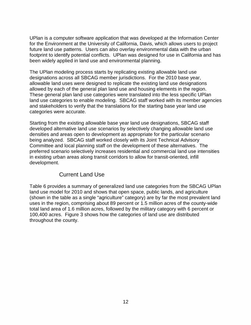
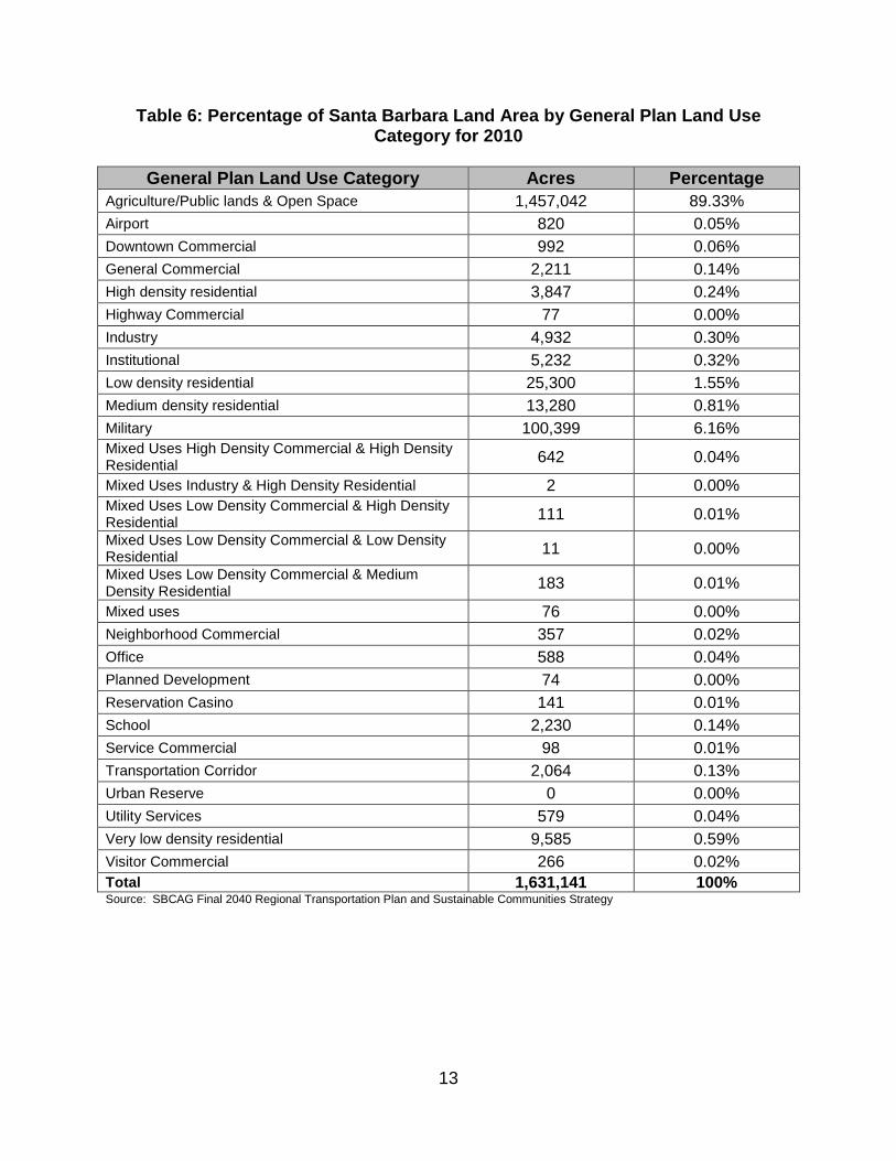
Current Land Use Table 6 provides a summary of generalized land use categories from the SBCAG UPlan land use model for 2010 and shows that open space, public lands, and agriculture (shown in the table as a single “agriculture” category) are by far the most prevalent land uses in the region, comprising about 89 percent or 1.5 million acres of the county-wide total land area of 1.6 million acres, followed by the military category with 6 percent or 100,400 acres. Figure 3 shows how the categories of land use are distributed throughout the county.

13

Table 6: Percentage of Santa Barbara Land Area by G eneral Plan Land Use Category for 2010

General Plan Land Use Category Acres Percentage Agriculture/Public lands & Open Space 1,457,042 89.33% Airport 820 0.05% Downtown Commercial 992 0.06% General Commercial 2,211 0.14% High density residential 3,847 0.24% Highway Commercial 77 0.00% Industry 4,932 0.30% Institutional 5,232 0.32% Low density residential 25,300 1.55% Medium density residential 13,280 0.81% Military 100,399 6.16% Mixed Uses High Density Commercial & High Density Residential 642 0.04%

Mixed Uses Industry & High Density Residential 2 0.00% Mixed Uses Low Density Commercial & High Density Residential 111 0.01%

Mixed Uses Low Density Commercial & Low Density Residential 11 0.00%

Mixed Uses Low Density Commercial & Medium Density Residential 183 0.01%

Mixed uses 76 0.00% Neighborhood Commercial 357 0.02% Office 588 0.04% Planned Development 74 0.00% Reservation Casino 141 0.01% School 2,230 0.14% Service Commercial 98 0.01% Transportation Corridor 2,064 0.13% Urban Reserve 0 0.00% Utility Services 579 0.04% Very low density residential 9,585 0.59% Visitor Commercial 266 0.02% Total 1,631,141 100% Source: SBCAG Final 2040 Regional Transportation Plan and Sustainable Communities Strategy

14

Figure 3: Santa Barbara Generalized Land Uses - 201 0

15

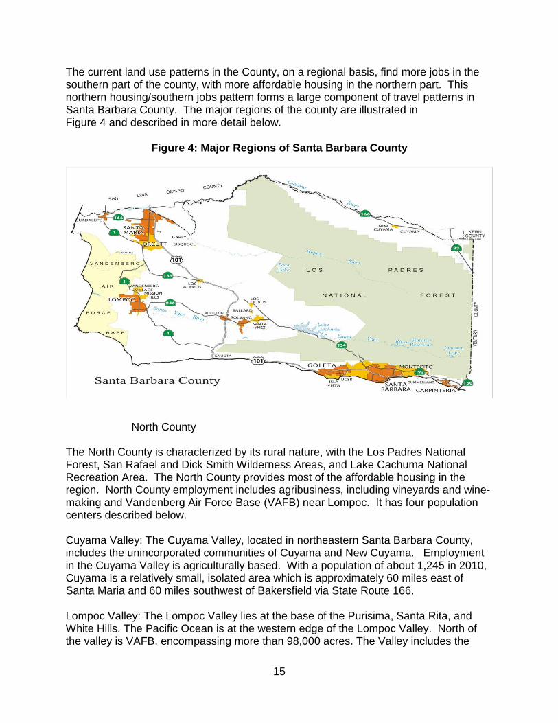
The current land use patterns in the County, on a regional basis, find more jobs in the southern part of the county, with more affordable housing in the northern part. This northern housing/southern jobs pattern forms a large component of travel patterns in Santa Barbara County. The major regions of the county are illustrated in Figure 4 and described in more detail below.

Figure 4: Major Regions of Santa Barbara County

North County The North County is characterized by its rural nature, with the Los Padres National Forest, San Rafael and Dick Smith Wilderness Areas, and Lake Cachuma National Recreation Area. The North County provides most of the affordable housing in the region. North County employment includes agribusiness, including vineyards and wine-making and Vandenberg Air Force Base (VAFB) near Lompoc. It has four population centers described below. Cuyama Valley: The Cuyama Valley, located in northeastern Santa Barbara County, includes the unincorporated communities of Cuyama and New Cuyama. Employment in the Cuyama Valley is agriculturally based. With a population of about 1,245 in 2010, Cuyama is a relatively small, isolated area which is approximately 60 miles east of Santa Maria and 60 miles southwest of Bakersfield via State Route 166. Lompoc Valley: The Lompoc Valley lies at the base of the Purisima, Santa Rita, and White Hills. The Pacific Ocean is at the western edge of the Lompoc Valley. North of the valley is VAFB, encompassing more than 98,000 acres. The Valley includes the

16

incorporated City of Lompoc, as well as Mission Hills, Mesa Oaks, and Vandenberg Village in unincorporated Santa Barbara County. Santa Maria Valley: The Santa Maria Valley is bounded by the Santa Maria River to the north, the Casmalia Hills to the west, and the Solomon Hills to the south. The Santa Maria Valley includes the cities of Santa Maria (the largest city in Santa Barbara County) and Guadalupe, and the unincorporated areas of Orcutt and Sisquoc. This is the fastest growing area of the county. Santa Ynez Valley: The Santa Ynez Valley lies at the base of several converging mountain ranges including the San Rafael and Santa Ynez Mountains and the Purisima and Santa Rita Hills. The Valley includes the incorporated cities of Buellton and Solvang, the small unincorporated communities of Ballard, Los Olivos, and Santa Ynez, and the Santa Ynez Band of Chumash Indians Reservation.

South Coast Bounded by the Santa Ynez Mountains to the north, the Pacific Ocean to the south, the Ventura County line to the east, and Gaviota to the west, is a narrow strip of coastal land known as the South Coast. It includes the incorporated cities of Carpinteria, Santa Barbara and Goleta, as well as unincorporated Summerland, Montecito, and Isla Vista.

Future Land Use –The Preferred Scenario The preferred scenario selected by SBCAG is a Transit-Oriented Development (TOD)/Infill plan. It selectively increases residential and commercial land use capacity within existing transit corridors shifting a greater share of future growth to these corridors. The preferred scenario shifts more housing growth to the South County to rely more heavily on transit and addresses the imbalance between jobs and housing in infill areas over time.

Assumed Land Use Changes The preferred scenario assumes changes to the land uses allowable under adopted general plans in selected areas to promote infill and transit-oriented development along existing transit routes within certain urbanized areas. In these core areas, residential and/or commercial densities are increased within close proximity to transit in order to facilitate transit, bike and walking trips.

Future Housing Patterns The SCS modeling process distinguishes between multi-family and single-family housing types based on underlying residential land use densities. Generally, the

17

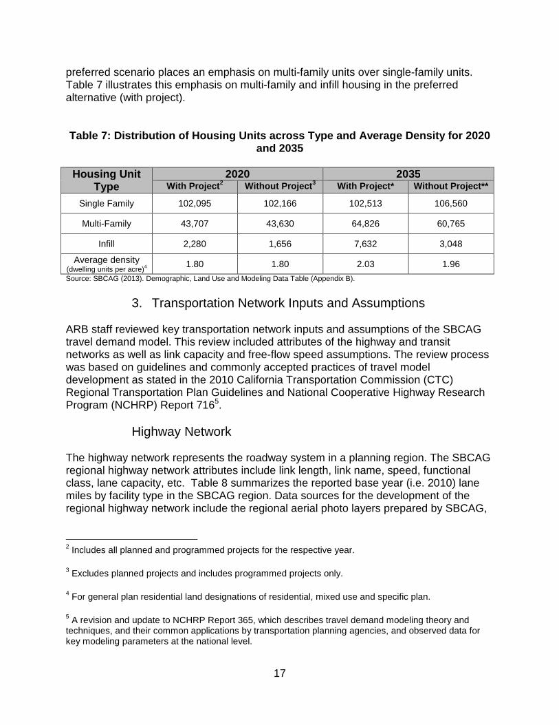
preferred scenario places an emphasis on multi-family units over single-family units. Table 7 illustrates this emphasis on multi-family and infill housing in the preferred alternative (with project).

Table 7: Distribution of Housing Units across Type and Average Density for 2020 and 2035

Housing Unit Type

2020 2035 With Project 2 Without Project 3 With Project * Without Project **

Single Family 102,095 102,166 102,513 106,560

Multi-Family 43,707 43,630 64,826 60,765

Infill 2,280 1,656 7,632 3,048

Average density (dwelling units per acre)4 1.80 1.80 2.03 1.96

Source: SBCAG (2013). Demographic, Land Use and Modeling Data Table (Appendix B).

3. Transportation Network Inputs and Assumptions

ARB staff reviewed key transportation network inputs and assumptions of the SBCAG travel demand model. This review included attributes of the highway and transit networks as well as link capacity and free-flow speed assumptions. The review process was based on guidelines and commonly accepted practices of travel model development as stated in the 2010 California Transportation Commission (CTC) Regional Transportation Plan Guidelines and National Cooperative Highway Research Program (NCHRP) Report 7165.

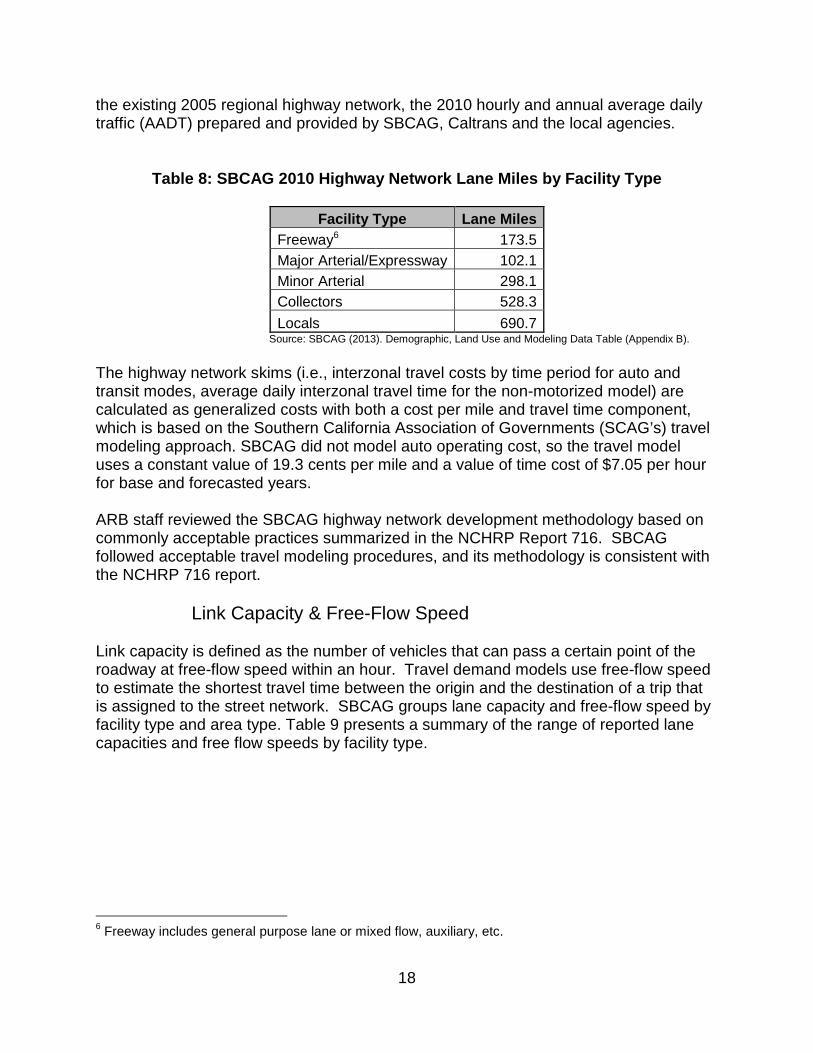
Highway Network The highway network represents the roadway system in a planning region. The SBCAG regional highway network attributes include link length, link name, speed, functional class, lane capacity, etc. Table 8 summarizes the reported base year (i.e. 2010) lane miles by facility type in the SBCAG region. Data sources for the development of the regional highway network include the regional aerial photo layers prepared by SBCAG,

2 Includes all planned and programmed projects for the respective year.

3 Excludes planned projects and includes programmed projects only.

4 For general plan residential land designations of residential, mixed use and specific plan.

5 A revision and update to NCHRP Report 365, which describes travel demand modeling theory and techniques, and their common applications by transportation planning agencies, and observed data for key modeling parameters at the national level.

18

the existing 2005 regional highway network, the 2010 hourly and annual average daily traffic (AADT) prepared and provided by SBCAG, Caltrans and the local agencies.

Table 8: SBCAG 2010 Highway Network Lane Miles by F acility Type

Facility Type Lane Miles Freeway6 173.5 Major Arterial/Expressway 102.1 Minor Arterial 298.1 Collectors 528.3

Locals 690.7 Source: SBCAG (2013). Demographic, Land Use and Modeling Data Table (Appendix B).

The highway network skims (i.e., interzonal travel costs by time period for auto and transit modes, average daily interzonal travel time for the non-motorized model) are calculated as generalized costs with both a cost per mile and travel time component, which is based on the Southern California Association of Governments (SCAG’s) travel modeling approach. SBCAG did not model auto operating cost, so the travel model uses a constant value of 19.3 cents per mile and a value of time cost of $7.05 per hour for base and forecasted years. ARB staff reviewed the SBCAG highway network development methodology based on commonly acceptable practices summarized in the NCHRP Report 716. SBCAG followed acceptable travel modeling procedures, and its methodology is consistent with the NCHRP 716 report.

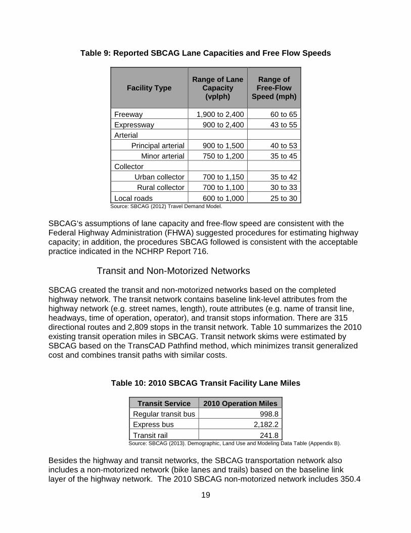
Link Capacity & Free-Flow Speed Link capacity is defined as the number of vehicles that can pass a certain point of the roadway at free-flow speed within an hour. Travel demand models use free-flow speed to estimate the shortest travel time between the origin and the destination of a trip that is assigned to the street network. SBCAG groups lane capacity and free-flow speed by facility type and area type. Table 9 presents a summary of the range of reported lane capacities and free flow speeds by facility type.

6 Freeway includes general purpose lane or mixed flow, auxiliary, etc.

19

Table 9: Reported SBCAG Lane Capacities and Free Fl ow Speeds

Facility Type Range of Lane

Capacity (vplph)

Range of Free-Flow

Speed (mph)

Freeway 1,900 to 2,400 60 to 65 Expressway 900 to 2,400 43 to 55 Arterial

Principal arterial 900 to 1,500 40 to 53 Minor arterial 750 to 1,200 35 to 45

Collector Urban collector 700 to 1,150 35 to 42 Rural collector 700 to 1,100 30 to 33

Local roads 600 to 1,000 25 to 30 Source: SBCAG (2012) Travel Demand Model.

SBCAG‘s assumptions of lane capacity and free-flow speed are consistent with the Federal Highway Administration (FHWA) suggested procedures for estimating highway capacity; in addition, the procedures SBCAG followed is consistent with the acceptable practice indicated in the NCHRP Report 716.

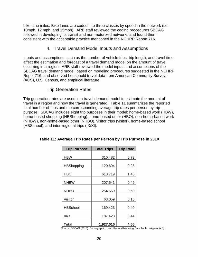
Transit and Non-Motorized Networks SBCAG created the transit and non-motorized networks based on the completed highway network. The transit network contains baseline link-level attributes from the highway network (e.g. street names, length), route attributes (e.g. name of transit line, headways, time of operation, operator), and transit stops information. There are 315 directional routes and 2,809 stops in the transit network. Table 10 summarizes the 2010 existing transit operation miles in SBCAG. Transit network skims were estimated by SBCAG based on the TransCAD Pathfind method, which minimizes transit generalized cost and combines transit paths with similar costs.

Table 10: 2010 SBCAG Transit Facility Lane Miles

Transit Service 2010 Operation Miles Regular transit bus 998.8 Express bus 2,182.2

Transit rail 241.8 Source: SBCAG (2013). Demographic, Land Use and Modeling Data Table (Appendix B). Besides the highway and transit networks, the SBCAG transportation network also includes a non-motorized network (bike lanes and trails) based on the baseline link layer of the highway network. The 2010 SBCAG non-motorized network includes 350.4

20

bike lane miles. Bike lanes are coded into three classes by speed in the network (i.e. 10mph, 12 mph, and 15mph). ARB staff reviewed the coding procedures SBCAG followed in developing its transit and non-motorized networks and found them consistent with the acceptable practice mentioned in the NCHRP Report 716.

4. Travel Demand Model Inputs and Assumptions Inputs and assumptions, such as the number of vehicle trips, trip length, and travel time, affect the estimation and forecast of a travel demand model on the amount of travel occurring in a region. ARB staff reviewed the model inputs and assumptions of the SBCAG travel demand model, based on modeling procedures suggested in the NCHRP Repot 716, and observed household travel data from American Community Surveys (ACS), U.S. Census, and empirical literature.

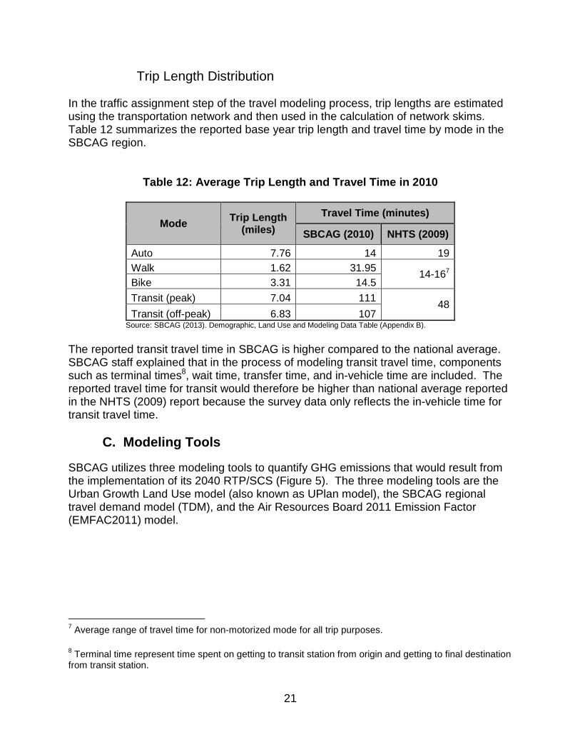
Trip Generation Rates Trip generation rates are used in a travel demand model to estimate the amount of travel in a region and how the travel is generated. Table 11 summarizes the reported total number of trips and the corresponding average trip rates per person by trip purpose. SBCAG includes eight trip purposes in their model: home-based work (HBW), home-based shopping (HBShopping), home-based other (HBO), non-home-based work (NHBW), non-home-based other (NHBO), visitor trips (visitor), home-based school (HBSchool), and inter-regional trips (IX/XI).

Table 11: Average Trip Rates per Person by Trip Pur pose in 2010

Trip Purpose Total Trips Trip Rate

HBW

310,482 0.73

HBShopping

120,694 0.28

HBO

613,719 1.45

NHBW

207,541 0.49

NHBO

254,669 0.60

Visitor

63,059 0.15

HBSchool

169,423 0.40

IX/XI

187,423 0.44

Total

1,927,010 4.55 Source: SBCAG (2013) Demographic, Land Use and Modeling Data Table. (Appendix B)

21

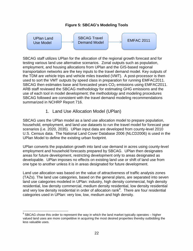
Trip Length Distribution In the traffic assignment step of the travel modeling process, trip lengths are estimated using the transportation network and then used in the calculation of network skims. Table 12 summarizes the reported base year trip length and travel time by mode in the SBCAG region.

Table 12: Average Trip Length and Travel Time in 20 10

Mode Trip Length (miles)

Travel Time (minutes)

SBCAG (2010) NHTS (2009)

Auto 7.76 14 19 Walk 1.62 31.95

14-167 Bike 3.31 14.5

Transit (peak) 7.04 111 48

Transit (off-peak) 6.83 107 Source: SBCAG (2013). Demographic, Land Use and Modeling Data Table (Appendix B). The reported transit travel time in SBCAG is higher compared to the national average. SBCAG staff explained that in the process of modeling transit travel time, components such as terminal times8, wait time, transfer time, and in-vehicle time are included. The reported travel time for transit would therefore be higher than national average reported in the NHTS (2009) report because the survey data only reflects the in-vehicle time for transit travel time.

C. Modeling Tools

SBCAG utilizes three modeling tools to quantify GHG emissions that would result from the implementation of its 2040 RTP/SCS (Figure 5). The three modeling tools are the Urban Growth Land Use model (also known as UPlan model), the SBCAG regional travel demand model (TDM), and the Air Resources Board 2011 Emission Factor (EMFAC2011) model.

7 Average range of travel time for non-motorized mode for all trip purposes.

8 Terminal time represent time spent on getting to transit station from origin and getting to final destination from transit station.

22

Figure 5: SBCAG’s Modeling Tools

SBCAG staff utilizes UPlan for the allocation of the regional growth forecast and for testing various land use alternative scenarios. Zonal outputs such as population, employment, and housing allocations from UPlan and the GIS-based regional transportation networks are the key inputs to the travel demand model. Key outputs of the TDM are vehicle trips and vehicle miles traveled (VMT). A post-processor is then used to sort the VMT outputs by speed class in preparation for running EMFAC2011. SBCAG then estimates base and forecasted years CO2 emissions using EMFAC2011. ARB staff reviewed the SBCAG methodology for estimating GHG emissions and the use of each tool in model development; the methodology and modeling procedures SBCAG followed are consistent with the travel demand modeling recommendations summarized in NCHRP Report 716.

1. Land Use Allocation Model (UPlan) SBCAG uses the UPlan model as a land use allocation model to prepare population, household, employment, and land use datasets to run the travel model for forecast year scenarios (i.e. 2020, 2035). UPlan input data are developed from county-level 2010 U.S. Census data. The National Land Cover Database 2006 (NLCD2006) is used in the UPlan Model to define the existing urban footprint. UPlan converts the population growth into land use demand in acres using county-level employment and household forecasts prepared by SBCAG. UPlan then designates areas for future development, restricting development only to areas designated as developable. UPlan imposes no effects on existing land use or shift of land use from one type to another unless it is in areas designated for future development. Land use allocation was based on the value of attractiveness of traffic analysis zones (TAZs). The land use categories, based on the general plans, are separated into seven land use categories modeled in UPlan: industry, high density commercial, high density residential, low density commercial, medium density residential, low density residential and very low density residential in order of allocation rank9. There are four residential categories used in UPlan: very low, low, medium and high density.

9 SBCAG chose this order to represent the way in which the land market typically operates – higher valued land uses are more competitive in acquiring the most desired properties thereby outbidding the less valuable uses.

EMFAC 2011 UPlan Land Use Model

SBCAG Travel Demand Model

23

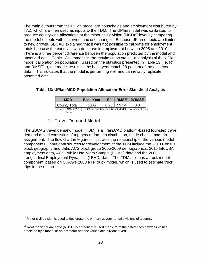
The main outputs from the UPlan model are households and employment distributed by TAZ, which are then used as inputs to the TDM. The UPlan model was calibrated to produce countywide allocations at the minor civil division (MCD)10 level by comparing the model outputs with observed land use changes. Because UPlan outputs are limited to new growth, SBCAG explained that it was not possible to calibrate for employment totals because the county saw a decrease in employment between 2005 and 2010. There is a three percent difference between the population predicted by the model and observed data. Table 13 summarizes the results of the statistical analysis of the UPlan model calibration on population. Based on the statistics presented in Table 13 (i.e. R2 and RMSE11 ), the model results in the base year match 98 percent of the observed data. This indicates that the model is performing well and can reliably replicate observed data.

Table 13: UPlan MCD Population Allocation Error Sta tistical Analysis

MCD Base Year R2 RMSE %RMSE

County Total 2005 0.98 597.4 0.3 Source: SBCAG (2012). SBCAG Land Use and Travel Model Development Final Report.

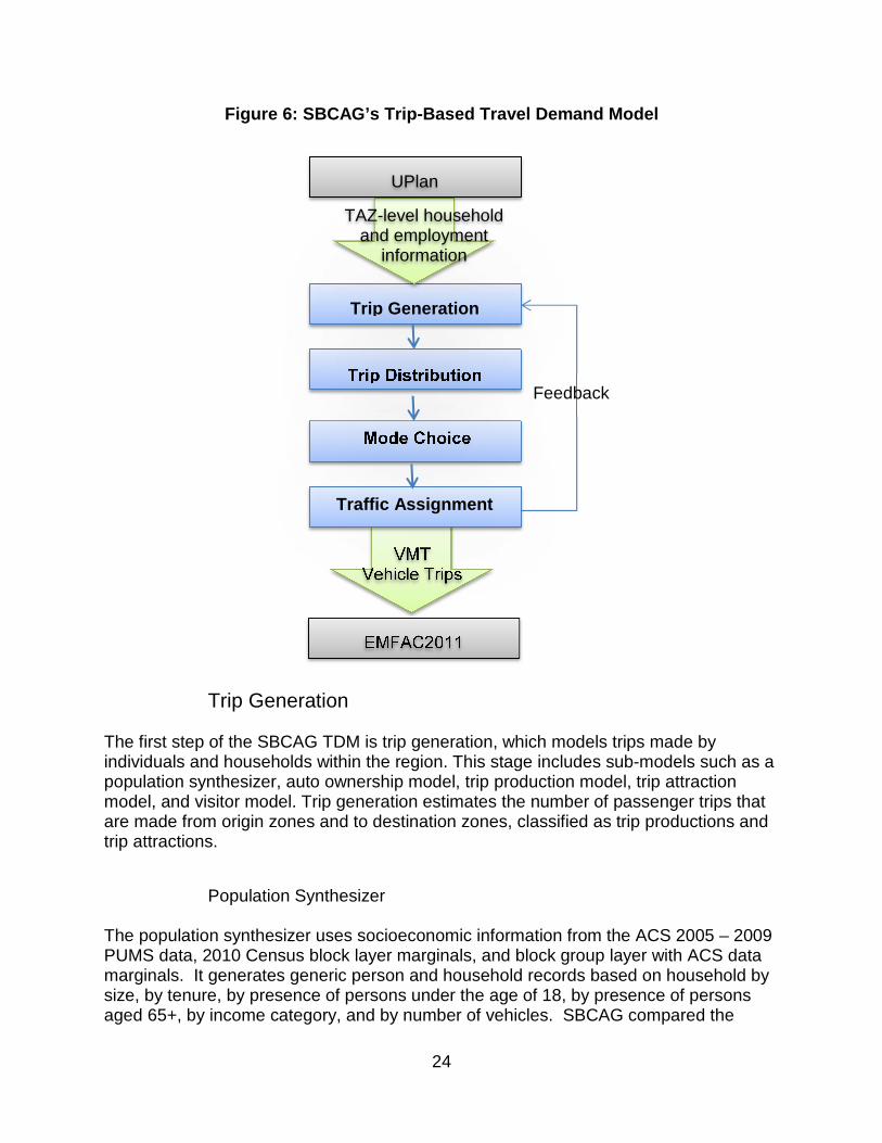
2. Travel Demand Model The SBCAG travel demand model (TDM) is a TransCAD platform-based four-step travel demand model consisting of trip generation, trip distribution, mode choice, and trip assignment. The flow chart in Figure 6 illustrates the relationship of the various model components. Input data sources for development of the TDM include the 2010 Census block geography and data, ACS block group 2005-2009 demographics, 2010 InfoUSA employment data, ACS Public Use Micro Sample (PUMS) data and the 2009 Longitudinal Employment Dynamics (LEHD) data. The TDM also has a truck model component, based on SCAG’s 2003 RTP truck model, which is used to estimate truck trips in the region.

10 Minor civil division is used to designate the primary governmental divisions of a county.

11 Root mean square error (RMSE) is a frequently used measure of the differences between values predicted by a model or an estimator and the values actually observed

24

Figure 6: SBCAG’s Trip-Based Travel Demand Model

Trip Generation The first step of the SBCAG TDM is trip generation, which models trips made by individuals and households within the region. This stage includes sub-models such as a population synthesizer, auto ownership model, trip production model, trip attraction model, and visitor model. Trip generation estimates the number of passenger trips that are made from origin zones and to destination zones, classified as trip productions and trip attractions.

Population Synthesizer The population synthesizer uses socioeconomic information from the ACS 2005 – 2009 PUMS data, 2010 Census block layer marginals, and block group layer with ACS data marginals. It generates generic person and household records based on household by size, by tenure, by presence of persons under the age of 18, by presence of persons aged 65+, by income category, and by number of vehicles. SBCAG compared the

EMFAC2011

VMT Vehicle Trips

Trip Distribution

Mode Choice

Traffic Assignment

Trip Generation

TAZ-level household and employment

information

UPlan

Feedback

25

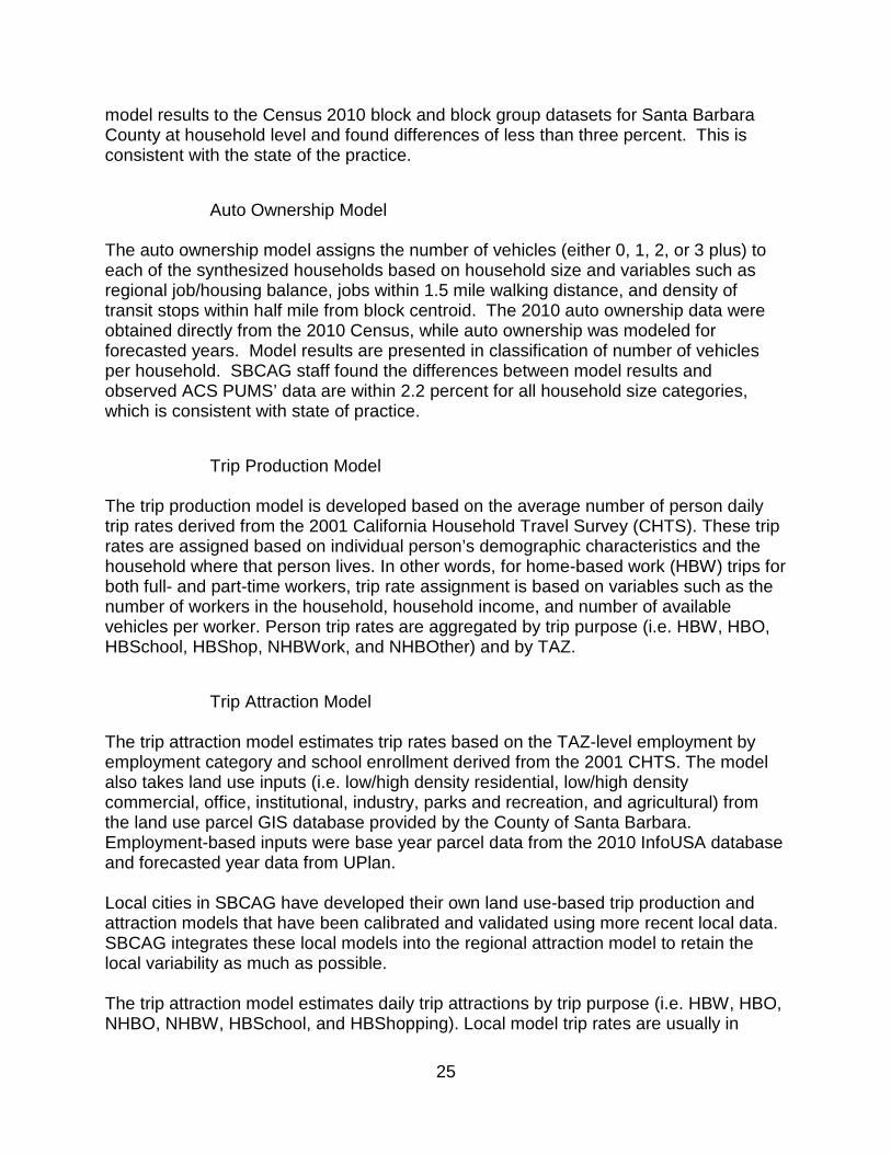
model results to the Census 2010 block and block group datasets for Santa Barbara County at household level and found differences of less than three percent. This is consistent with the state of the practice.

Auto Ownership Model The auto ownership model assigns the number of vehicles (either 0, 1, 2, or 3 plus) to each of the synthesized households based on household size and variables such as regional job/housing balance, jobs within 1.5 mile walking distance, and density of transit stops within half mile from block centroid. The 2010 auto ownership data were obtained directly from the 2010 Census, while auto ownership was modeled for forecasted years. Model results are presented in classification of number of vehicles per household. SBCAG staff found the differences between model results and observed ACS PUMS’ data are within 2.2 percent for all household size categories, which is consistent with state of practice.

Trip Production Model The trip production model is developed based on the average number of person daily trip rates derived from the 2001 California Household Travel Survey (CHTS). These trip rates are assigned based on individual person’s demographic characteristics and the household where that person lives. In other words, for home-based work (HBW) trips for both full- and part-time workers, trip rate assignment is based on variables such as the number of workers in the household, household income, and number of available vehicles per worker. Person trip rates are aggregated by trip purpose (i.e. HBW, HBO, HBSchool, HBShop, NHBWork, and NHBOther) and by TAZ.

Trip Attraction Model The trip attraction model estimates trip rates based on the TAZ-level employment by employment category and school enrollment derived from the 2001 CHTS. The model also takes land use inputs (i.e. low/high density residential, low/high density commercial, office, institutional, industry, parks and recreation, and agricultural) from the land use parcel GIS database provided by the County of Santa Barbara. Employment-based inputs were base year parcel data from the 2010 InfoUSA database and forecasted year data from UPlan. Local cities in SBCAG have developed their own land use-based trip production and attraction models that have been calibrated and validated using more recent local data. SBCAG integrates these local models into the regional attraction model to retain the local variability as much as possible. The trip attraction model estimates daily trip attractions by trip purpose (i.e. HBW, HBO, NHBO, NHBW, HBSchool, and HBShopping). Local model trip rates are usually in

26

vehicle trips; SBCAG converts them into person trip rates by applying auto occupancy factors derived from the 2001 CHTS.

Visitor Model The trip generation step of the SBCAG TDM includes a model to estimate trips made by day and overnight visitors. The trip production rates of visitors were estimated based on a 2008 Santa Barbara County Visitor Survey and an earlier version of the SBCAG TDM, which used information from a visitor survey conducted in Monterey County. On average, an overnight visitor makes about 4 trips per day, while a day visitor makes about 2.4 trips per day. Visitor productions were determined based on variables such as households, hotel/motel, and service employment. The trip attraction rates of visitors were derived based on households, service employment, and commercial employment. Survey data show that 14.7 percent of visitors visit homes of relatives.

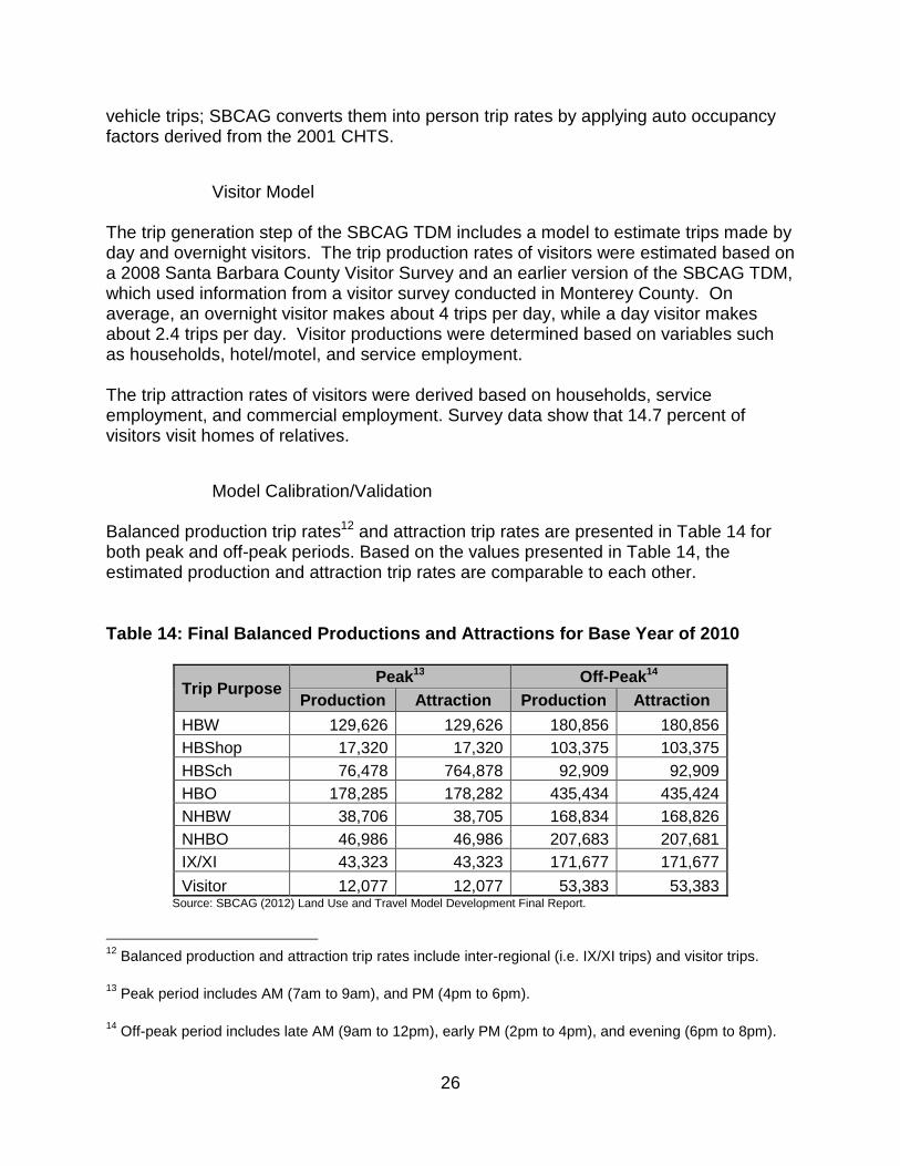
Model Calibration/Validation Balanced production trip rates12 and attraction trip rates are presented in Table 14 for both peak and off-peak periods. Based on the values presented in Table 14, the estimated production and attraction trip rates are comparable to each other.

Table 14: Final Balanced Productions and Attraction s for Base Year of 2010

Trip Purpose Peak13 Off-Peak 14

Production Attraction Production Attraction

HBW 129,626 129,626 180,856 180,856 HBShop 17,320 17,320 103,375 103,375 HBSch 76,478 764,878 92,909 92,909 HBO 178,285 178,282 435,434 435,424 NHBW 38,706 38,705 168,834 168,826 NHBO 46,986 46,986 207,683 207,681 IX/XI 43,323 43,323 171,677 171,677

Visitor 12,077 12,077 53,383 53,383 Source: SBCAG (2012) Land Use and Travel Model Development Final Report.

12 Balanced production and attraction trip rates include inter-regional (i.e. IX/XI trips) and visitor trips.

13 Peak period includes AM (7am to 9am), and PM (4pm to 6pm).

14 Off-peak period includes late AM (9am to 12pm), early PM (2pm to 4pm), and evening (6pm to 8pm).

27

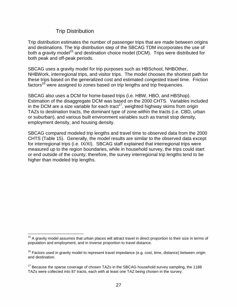
Trip Distribution Trip distribution estimates the number of passenger trips that are made between origins and destinations. The trip distribution step of the SBCAG TDM incorporates the use of both a gravity model15 and destination choice model (DCM). Trips were distributed for both peak and off-peak periods. SBCAG uses a gravity model for trip purposes such as HBSchool, NHBOther, NHBWork, interregional trips, and visitor trips. The model chooses the shortest path for these trips based on the generalized cost and estimated congested travel time. Friction factors16 were assigned to zones based on trip lengths and trip frequencies. SBCAG also uses a DCM for home-based trips (i.e. HBW, HBO, and HBShop). Estimation of the disaggregate DCM was based on the 2000 CHTS. Variables included in the DCM are a size variable for each tract17, weighted highway skims from origin TAZs to destination tracts, the dominant type of zone within the tracts (i.e. CBD, urban or suburban), and various built environment variables such as transit stop density, employment density, and housing density. SBCAG compared modeled trip lengths and travel time to observed data from the 2000 CHTS (Table 15). Generally, the model results are similar to the observed data except for interregional trips (i.e. IX/XI). SBCAG staff explained that interregional trips were measured up to the region boundaries, while in household survey, the trips could start or end outside of the county; therefore, the survey interregional trip lengths tend to be higher than modeled trip lengths.

15 A gravity model assumes that urban places will attract travel in direct proportion to their size in terms of population and employment, and in inverse proportion to travel distance.

16 Factors used in gravity model to represent travel impedance (e.g. cost, time, distance) between origin and destination.

17 Because the sparse coverage of chosen TAZs in the SBCAG household survey sampling, the 1188 TAZs were collected into 87 tracts, each with at least one TAZ being chosen in the survey.

28

Table 15: Survey and Model Trip Lengths and Travel Time for 2010

Purpose Peak Distance

(miles) Peak Time (minutes)

Off -peak Distance (miles)

Off -peak Time (minutes)

Survey Model Survey Model Survey Model Survey Model

HBW 7.6 8.3 14.9 15 7.3 8.6 14.2 15.3 HBShop 4.7 4.4 11 10.4 4.1 4.5 10.2 10.3 HBSchool 5.3 5.3 11.6 12 4.3 7.5 10.2 10.3 HBO 4.5 4.9 10.7 11.1 4.5 5 10.4 11 NHBW 7.1 6.6 13.9 13.1 5.9 5.6 12.2 11.7 NHBO 4.2 6.4 9.8 12.2 3.3 4 8.6 9.4

IX/XI 35.6 28.6 46.4 37.8 29.2 25.8 38.9 33.7 Source: SBCAG (2012) Land Use and Travel Model Development Final Report.

Mode Choice

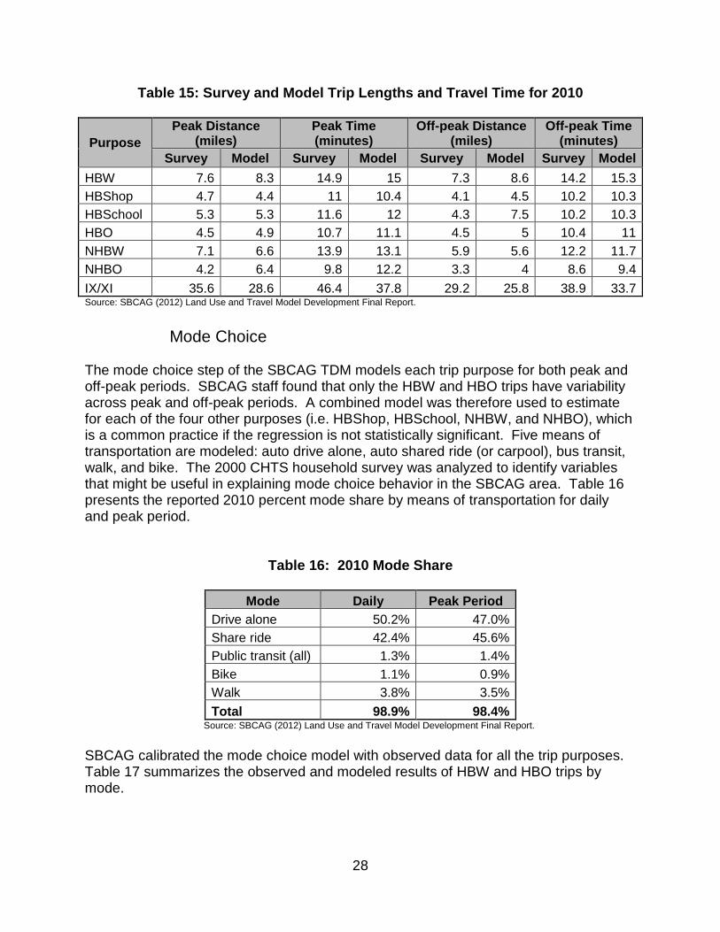
The mode choice step of the SBCAG TDM models each trip purpose for both peak and off-peak periods. SBCAG staff found that only the HBW and HBO trips have variability across peak and off-peak periods. A combined model was therefore used to estimate for each of the four other purposes (i.e. HBShop, HBSchool, NHBW, and NHBO), which is a common practice if the regression is not statistically significant. Five means of transportation are modeled: auto drive alone, auto shared ride (or carpool), bus transit, walk, and bike. The 2000 CHTS household survey was analyzed to identify variables that might be useful in explaining mode choice behavior in the SBCAG area. Table 16 presents the reported 2010 percent mode share by means of transportation for daily and peak period.

Table 16: 2010 Mode Share

Mode Daily Peak Period Drive alone 50.2% 47.0% Share ride 42.4% 45.6% Public transit (all) 1.3% 1.4% Bike 1.1% 0.9% Walk 3.8% 3.5%

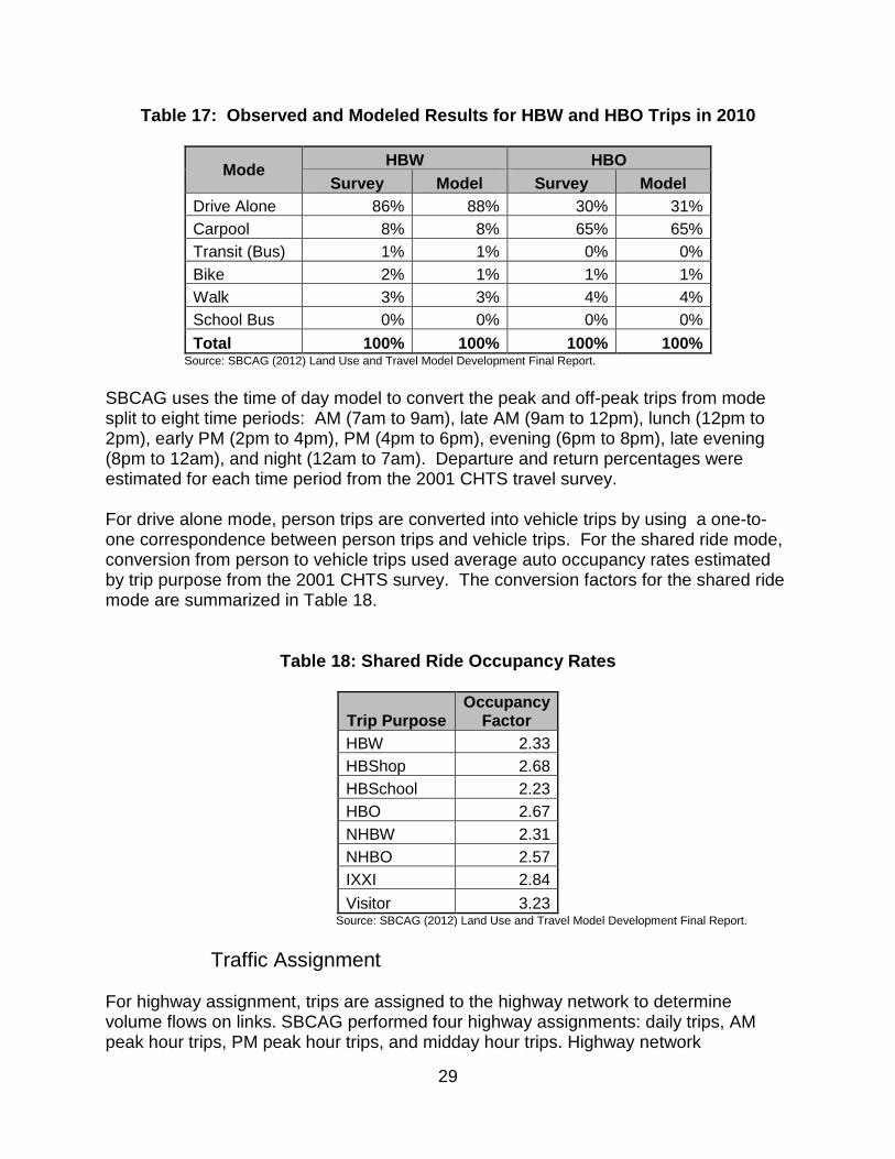
Total 98.9% 98.4% Source: SBCAG (2012) Land Use and Travel Model Development Final Report. SBCAG calibrated the mode choice model with observed data for all the trip purposes. Table 17 summarizes the observed and modeled results of HBW and HBO trips by mode.

29

Table 17: Observed and Modeled Results for HBW and HBO Trips in 2010

Mode HBW HBO

Survey Model Survey Model Drive Alone 86% 88% 30% 31% Carpool 8% 8% 65% 65% Transit (Bus) 1% 1% 0% 0% Bike 2% 1% 1% 1% Walk 3% 3% 4% 4% School Bus 0% 0% 0% 0%

Total 100% 100% 100% 100% Source: SBCAG (2012) Land Use and Travel Model Development Final Report. SBCAG uses the time of day model to convert the peak and off-peak trips from mode split to eight time periods: AM (7am to 9am), late AM (9am to 12pm), lunch (12pm to 2pm), early PM (2pm to 4pm), PM (4pm to 6pm), evening (6pm to 8pm), late evening (8pm to 12am), and night (12am to 7am). Departure and return percentages were estimated for each time period from the 2001 CHTS travel survey. For drive alone mode, person trips are converted into vehicle trips by using a one-to-one correspondence between person trips and vehicle trips. For the shared ride mode, conversion from person to vehicle trips used average auto occupancy rates estimated by trip purpose from the 2001 CHTS survey. The conversion factors for the shared ride mode are summarized in Table 18.

Table 18: Shared Ride Occupancy Rates

Trip Purpose Occupancy

Factor HBW 2.33 HBShop 2.68 HBSchool 2.23 HBO 2.67 NHBW 2.31 NHBO 2.57 IXXI 2.84

Visitor 3.23 Source: SBCAG (2012) Land Use and Travel Model Development Final Report.

Traffic Assignment For highway assignment, trips are assigned to the highway network to determine volume flows on links. SBCAG performed four highway assignments: daily trips, AM peak hour trips, PM peak hour trips, and midday hour trips. Highway network

30

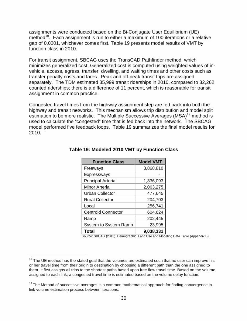
assignments were conducted based on the Bi-Conjugate User Equilibrium (UE) method18. Each assignment is run to either a maximum of 100 iterations or a relative gap of 0.0001, whichever comes first. Table 19 presents model results of VMT by function class in 2010. For transit assignment, SBCAG uses the TransCAD Pathfinder method, which minimizes generalized cost. Generalized cost is computed using weighted values of in-vehicle, access, egress, transfer, dwelling, and waiting times and other costs such as transfer penalty costs and fares. Peak and off-peak transit trips are assigned separately. The TDM estimated 35,999 transit riderships in 2010, compared to 32,262 counted riderships; there is a difference of 11 percent, which is reasonable for transit assignment in common practice. Congested travel times from the highway assignment step are fed back into both the highway and transit networks. This mechanism allows trip distribution and model split estimation to be more realistic. The Multiple Successive Averages (MSA)19 method is used to calculate the “congested” time that is fed back into the network. The SBCAG model performed five feedback loops. Table 19 summarizes the final model results for 2010.

Table 19: Modeled 2010 VMT by Function Class

Function Class Model VMT Freeways 3,868,810 Expressways - Principal Arterial 1,336,093 Minor Arterial 2,063,275 Urban Collector 477,645 Rural Collector 204,703 Local 256,741 Centroid Connector 604,624 Ramp 202,445 System to System Ramp 23,995

Total 9,038,331 Source: SBCAG (2013). Demographic, Land Use and Modeling Data Table (Appendix B).

18 The UE method has the stated goal that the volumes are estimated such that no user can improve his or her travel time from their origin to destination by choosing a different path than the one assigned to them. It first assigns all trips to the shortest paths based upon free flow travel time. Based on the volume assigned to each link, a congested travel time is estimated based on the volume delay function.

19 The Method of successive averages is a common mathematical approach for finding convergence in link volume estimation process between iterations.

31

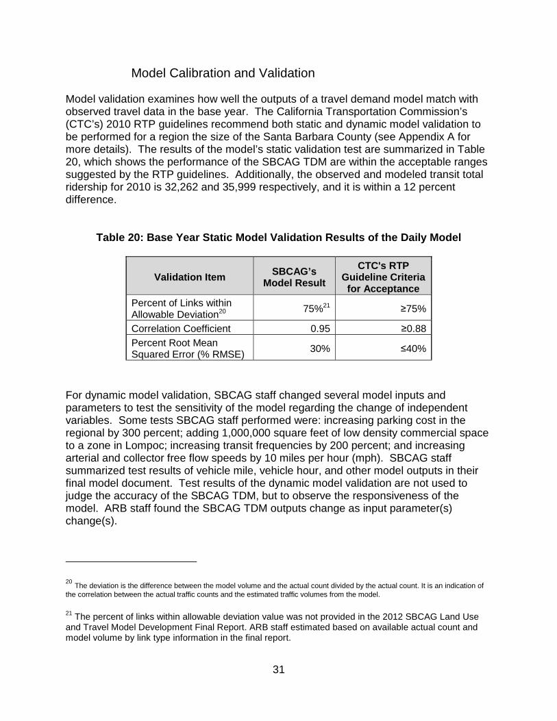
Model Calibration and Validation Model validation examines how well the outputs of a travel demand model match with observed travel data in the base year. The California Transportation Commission’s (CTC’s) 2010 RTP guidelines recommend both static and dynamic model validation to be performed for a region the size of the Santa Barbara County (see Appendix A for more details). The results of the model’s static validation test are summarized in Table 20, which shows the performance of the SBCAG TDM are within the acceptable ranges suggested by the RTP guidelines. Additionally, the observed and modeled transit total ridership for 2010 is 32,262 and 35,999 respectively, and it is within a 12 percent difference.

Table 20: Base Year Static Model Validation Results of the Daily Model

Validation Item SBCAG’s Model Result

CTC's RTP Guideline Criteria for Acceptance

Percent of Links within Allowable Deviation20 75%21 ≥75%

Correlation Coefficient 0.95 ≥0.88 Percent Root Mean Squared Error (% RMSE) 30% ≤40%

For dynamic model validation, SBCAG staff changed several model inputs and parameters to test the sensitivity of the model regarding the change of independent variables. Some tests SBCAG staff performed were: increasing parking cost in the regional by 300 percent; adding 1,000,000 square feet of low density commercial space to a zone in Lompoc; increasing transit frequencies by 200 percent; and increasing arterial and collector free flow speeds by 10 miles per hour (mph). SBCAG staff summarized test results of vehicle mile, vehicle hour, and other model outputs in their final model document. Test results of the dynamic model validation are not used to judge the accuracy of the SBCAG TDM, but to observe the responsiveness of the model. ARB staff found the SBCAG TDM outputs change as input parameter(s) change(s).

20 The deviation is the difference between the model volume and the actual count divided by the actual count. It is an indication of the correlation between the actual traffic counts and the estimated traffic volumes from the model.

21 The percent of links within allowable deviation value was not provided in the 2012 SBCAG Land Use and Travel Model Development Final Report. ARB staff estimated based on available actual count and model volume by link type information in the final report.

32

3. EMFAC Model The ARB Emission Factor model (EMFAC2011) is a California-specific computer model which calculates weekday emissions of air pollutants from all on-road motor vehicles including passenger cars, trucks, and buses for calendar years 1990 to 2035. The model estimates exhaust and evaporative hydrocarbons, carbon monoxide, oxides of nitrogen, particulate matter, oxides of sulfur, methane, and CO2 emissions. It uses vehicle activity provided by regional transportation planning agencies, and emission rates developed from testing of in-use vehicles. The model estimates emissions at the statewide, county, air district, and air basin levels. The EMFAC2011 modeling package contains three components: EMFAC2011-LDV for light-duty vehicles, EMFAC2011-HD for heavy-duty vehicles, and EMFAC2011-SG for future growth scenarios. SBCAG inputs the estimated VMT by speed bin to EMFAC 2011 to estimate GHG emissions for baseline as well as forecasted years for its SCS preferred scenario. The GHG emissions estimates are presented as tons of CO2 per day. The estimated total weekday CO2 emissions for year 2005, 2010, 2020, and 2035 were converted to per capita CO2 emissions.

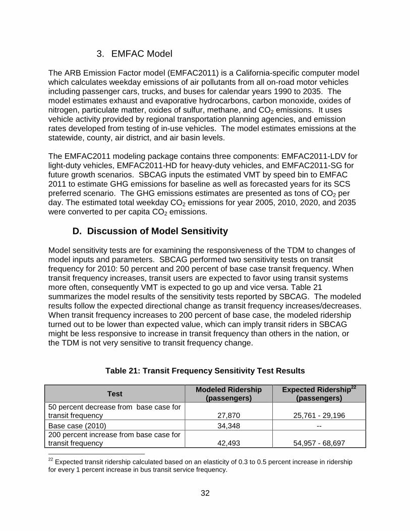
D. Discussion of Model Sensitivity Model sensitivity tests are for examining the responsiveness of the TDM to changes of model inputs and parameters. SBCAG performed two sensitivity tests on transit frequency for 2010: 50 percent and 200 percent of base case transit frequency. When transit frequency increases, transit users are expected to favor using transit systems more often, consequently VMT is expected to go up and vice versa. Table 21 summarizes the model results of the sensitivity tests reported by SBCAG. The modeled results follow the expected directional change as transit frequency increases/decreases. When transit frequency increases to 200 percent of base case, the modeled ridership turned out to be lower than expected value, which can imply transit riders in SBCAG might be less responsive to increase in transit frequency than others in the nation, or the TDM is not very sensitive to transit frequency change.

Table 21: Transit Frequency Sensitivity Test Result s

Test Modeled Ridership (passengers)

Expected Ridership 22 (passengers)

50 percent decrease from base case for transit frequency 27,870 25,761 - 29,196 Base case (2010) 34,348 -- 200 percent increase from base case for transit frequency 42,493 54,957 - 68,697 22 Expected transit ridership calculated based on an elasticity of 0.3 to 0.5 percent increase in ridership for every 1 percent increase in bus transit service frequency.

33

IV. PERFORMANCE INDICATORS

A. Land Use – Residential Density Residential density is a measure of the average number of dwelling units per acre of developed land. The SBCAG SCS anticipates a change in travel characteristics in the region as the housing market shifts from single family to multi-family housing. These changes in travel behavior include reductions in average trip length and decreased regional VMT. SBCAG SCS land use plan includes residential densities sufficient to accommodate projected population and household growth. The region has planned for significant additional new housing in urbanized areas on the South Coast near employment centers and accessible to transit. These efforts help to improve the regional jobs/housing imbalance and reduce long-distance commuting. The Santa Barbara region has approximately 142,100 housing units assumed in the 2010 base case, with roughly 70 percent single-family and 30 percent multi-family. Total housing units increase approximately 18 percent with the SCS in 2035, with roughly 60 percent single-family and 40 percent multi-family. The SBCAG SCS reports an average residential density of 1.76 units per acre in 2010 increasing to 2.03 in 2035. This represents an increase of 0.27 housing units per acre (or 15 percent) between 2010 and 2035. During the same period, the Santa Barbara SCS also reports a regional per capita VMT decrease of 9.6 percent. A review of relevant empirical literature supports the SBCAG finding that decreased regional VMT should result from increased residential density. Brownstone and Golob analyzed National Household Travel Survey (NHTS) data and observed that denser housing development significantly reduces annual vehicle mileage and fuel consumption, which directly results in the reduction in GHG emissions. They also reported that households in areas with 1,000 or more units per square mile drive 1,171 fewer miles and consume 64.7 fewer gallons of fuel than households in less dense areas. Boarnet and Handy (2010) reported that doubling residential density reduces VMT an average of 5 to 12 percent. Manville and Shoup (2005) reported that a 1 percent population density increase is associated with a 0.58 percent reduction in VMT in a survey of twenty urbanized areas. As Boarnet and Handy (2010) report, due to the urban focus in the literature, it is important to note that there is little evidence that explores in any specificity on the way that residential density interacts with VMT in rural areas. While the levels of increased residential density in SBCAG are relatively low, they are directionally consistent with what the literature would indicate as resulting in reduced vehicle miles traveled and greenhouse gas emissions.

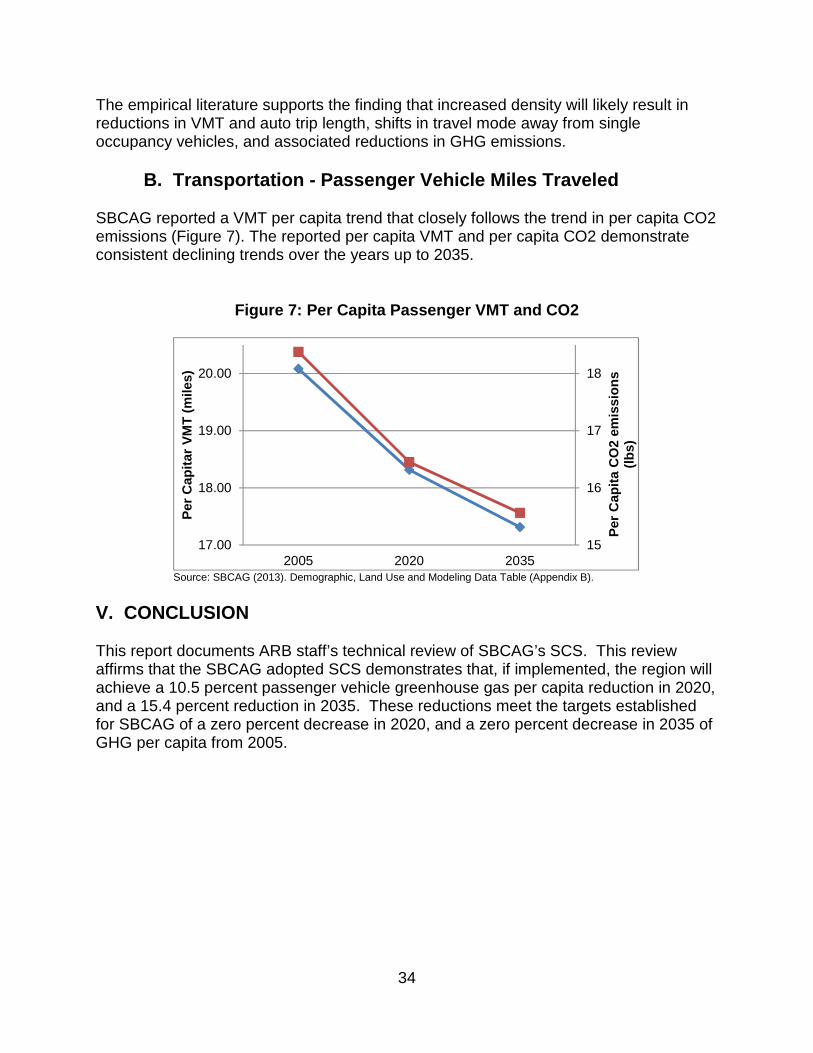
34

The empirical literature supports the finding that increased density will likely result in reductions in VMT and auto trip length, shifts in travel mode away from single occupancy vehicles, and associated reductions in GHG emissions.

B. Transportation - Passenger Vehicle Miles Travel ed SBCAG reported a VMT per capita trend that closely follows the trend in per capita CO2 emissions (Figure 7). The reported per capita VMT and per capita CO2 demonstrate consistent declining trends over the years up to 2035.

Figure 7: Per Capita Passenger VMT and CO2

Source: SBCAG (2013). Demographic, Land Use and Modeling Data Table (Appendix B). V. CONCLUSION This report documents ARB staff’s technical review of SBCAG’s SCS. This review affirms that the SBCAG adopted SCS demonstrates that, if implemented, the region will achieve a 10.5 percent passenger vehicle greenhouse gas per capita reduction in 2020, and a 15.4 percent reduction in 2035. These reductions meet the targets established for SBCAG of a zero percent decrease in 2020, and a zero percent decrease in 2035 of GHG per capita from 2005.

15

16

17

18

17.00

18.00

19.00

20.00

2005 2020 2035

Per

Cap

ita C

O2

emis

sion

s (lb

s)

Per

Cap

itar

VM

T (m

iles)

35

VI. REFERENCES Boarnet, Marlon G., and Susan Handy (2010) “Draft Policy Brief on the Impact of

Residential Density Based on a Review of the Empirical Literature.” Accessed 6 December 2012 at http://www.arb.ca.gov/cc/sb375/policies/density/density_brief.pdf

Brownstone, David and Thomas Golob (2009) The Impact of Residential Density on

Vehicle Usage and Energy Consumption. Journal of Urban Economics 65: 91- 98.

California Air Resources Board (CARB) (2011) Description of Methodology for ARB

Staff Review of Greenhouse Gas Reductions from Sustainable Communities Strategies (SCS) Pursuant to SB 375. Access 2013 at http://www.arb.ca.gov/cc/sb375/scs_review_methodology.pdf

California Air Resources Board (2010) EMFAC2007 User’s Guide: Calculating Emission

Inventories for Vehicle in California. Accessed December 7 2012 at http://www.arb.ca.gov/msei/onroad/downloads/docs/user_guide_emfac2007.pdf.

California Transportation Commission (2010). Regional Transportation Plan Guidelines.

Assessed 6 December 2012 at http://www.catc.ca.gov/programs/rtp/2010_RTP_Guidelines.pdf.

Caliper (2012). SBCAG Land Use and Travel Model Development Final Report.

Prepared for Santa Barbara Association of Governments (SBCAG). Caliper (2008) Travel Demand Modeling with TransCAD 5.0: User’s Guide. Federal Highway Administration (FHWA) (2011) HPMS Field Manual – Appendix N:

Procedures for Estimating Highway Capacity. Accessed 2013 at https://www.fhwa.dot.gov/ohim/hpmsmanl/appn1.cfm.

Handy, Susan, Steve Spears, and Marlon G. Boarnet (2010). Draft Policy Brief on the

Impacts of Transit Service Strategies Based on a Review of the Empirical Literature. Accessed 2013 at http://www.arb.ca.gov/cc/sb375/policies/transitservice/transitservice_brief.pdf.

Manville, Michael & Shoup, Donald. (2005) “Parking, People, and Cities.” Journal of

Urban Planning and Development: 233-245. Accessed 7 December 2012 at http://shoup.bol.ucla.edu/People,Parking,CitiesJUPD.pdf

Santa Barbara Association of Governments (SBCAG) (2013). Demographic, Land Use

and Modeling Data Table for SBCAG. Spread sheet submittal to the California Air Resource Board.

36

Santa Barbara Association of Governments (SBCAG) (2013) Final 2040 Regional

Transportation Plan and Sustainable Communities Strategy. Access 2013 at http://www.sbcag.org/planning/2040RTP/Documents.html

Santa Barbara Association of Governments (SBCAG) (2012) Regional Growth Forecast

2010 – 2040. Accessed May 2013 at http://www.sbcag.org/PDFs/publications/Final%202040%20Regional%20Growth%20Forecast.pdf.

Santa Barbara Association of Governments (SBCAG) (2011) Technical Methodology

Estimating Greenhouse Gas Emissions in the Sustainable Communities Strategy. Accessed May 2013 at http://www.sbcag.org/planning/2040RTP/images_docs/SCS%20Technical%20Methodology.pdf.

Transportation Research Board (2012) NCHRP Report 716: Travel Demand

Forecasting – Parameters and Techniques. Accessed August 2013 at http://onlinepubs.trb.org/onlinepubs/nchrp/nchrp_rpt_716.pdf.

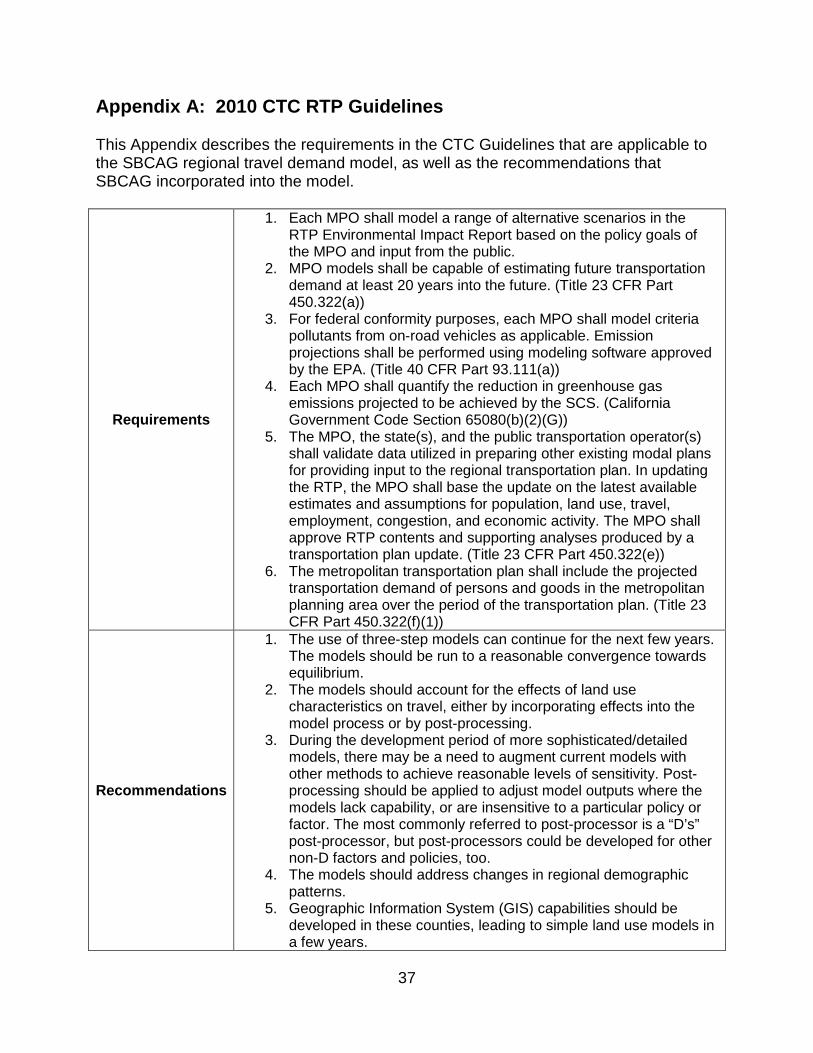
37

Appendix A: 2010 CTC RTP Guidelines This Appendix describes the requirements in the CTC Guidelines that are applicable to the SBCAG regional travel demand model, as well as the recommendations that SBCAG incorporated into the model.

Requirements

1. Each MPO shall model a range of alternative scenarios in the RTP Environmental Impact Report based on the policy goals of the MPO and input from the public.

2. MPO models shall be capable of estimating future transportation demand at least 20 years into the future. (Title 23 CFR Part 450.322(a))

3. For federal conformity purposes, each MPO shall model criteria pollutants from on-road vehicles as applicable. Emission projections shall be performed using modeling software approved by the EPA. (Title 40 CFR Part 93.111(a))

4. Each MPO shall quantify the reduction in greenhouse gas emissions projected to be achieved by the SCS. (California Government Code Section 65080(b)(2)(G))

5. The MPO, the state(s), and the public transportation operator(s) shall validate data utilized in preparing other existing modal plans for providing input to the regional transportation plan. In updating the RTP, the MPO shall base the update on the latest available estimates and assumptions for population, land use, travel, employment, congestion, and economic activity. The MPO shall approve RTP contents and supporting analyses produced by a transportation plan update. (Title 23 CFR Part 450.322(e))

6. The metropolitan transportation plan shall include the projected transportation demand of persons and goods in the metropolitan planning area over the period of the transportation plan. (Title 23 CFR Part 450.322(f)(1))

Recommendations

1. The use of three-step models can continue for the next few years. The models should be run to a reasonable convergence towards equilibrium.

2. The models should account for the effects of land use characteristics on travel, either by incorporating effects into the model process or by post-processing.

3. During the development period of more sophisticated/detailed models, there may be a need to augment current models with other methods to achieve reasonable levels of sensitivity. Post-processing should be applied to adjust model outputs where the models lack capability, or are insensitive to a particular policy or factor. The most commonly referred to post-processor is a “D’s” post-processor, but post-processors could be developed for other non-D factors and policies, too.

4. The models should address changes in regional demographic patterns.

5. Geographic Information System (GIS) capabilities should be developed in these counties, leading to simple land use models in a few years.

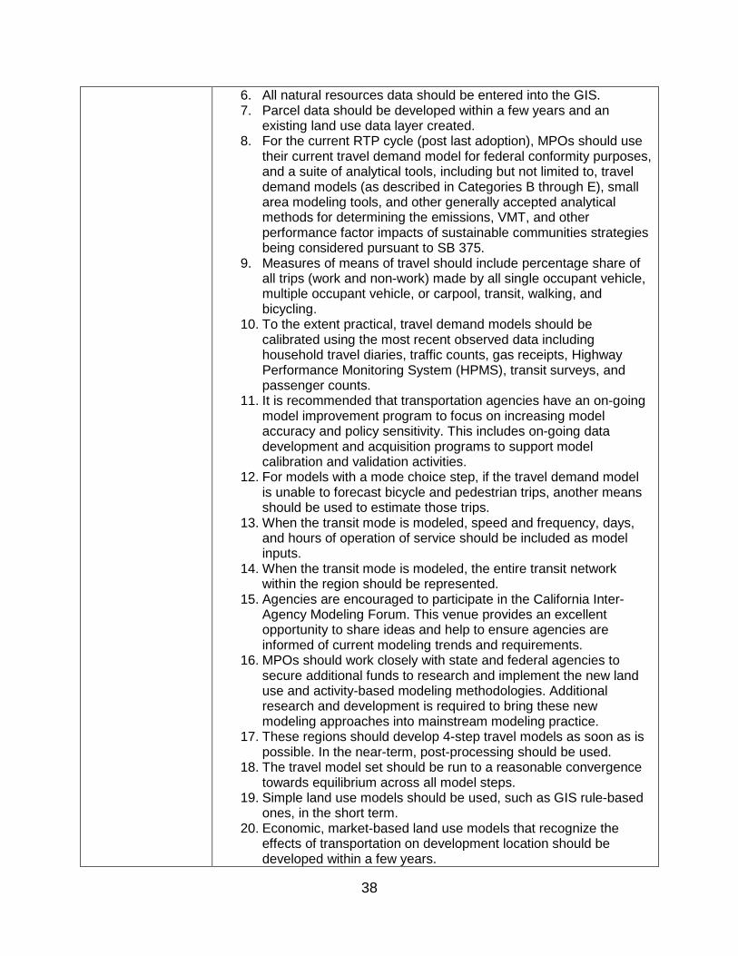
38

6. All natural resources data should be entered into the GIS. 7. Parcel data should be developed within a few years and an

existing land use data layer created. 8. For the current RTP cycle (post last adoption), MPOs should use

their current travel demand model for federal conformity purposes, and a suite of analytical tools, including but not limited to, travel demand models (as described in Categories B through E), small area modeling tools, and other generally accepted analytical methods for determining the emissions, VMT, and other performance factor impacts of sustainable communities strategies being considered pursuant to SB 375.

9. Measures of means of travel should include percentage share of all trips (work and non-work) made by all single occupant vehicle, multiple occupant vehicle, or carpool, transit, walking, and bicycling.

10. To the extent practical, travel demand models should be calibrated using the most recent observed data including household travel diaries, traffic counts, gas receipts, Highway Performance Monitoring System (HPMS), transit surveys, and passenger counts.

11. It is recommended that transportation agencies have an on-going model improvement program to focus on increasing model accuracy and policy sensitivity. This includes on-going data development and acquisition programs to support model calibration and validation activities.

12. For models with a mode choice step, if the travel demand model is unable to forecast bicycle and pedestrian trips, another means should be used to estimate those trips.

13. When the transit mode is modeled, speed and frequency, days, and hours of operation of service should be included as model inputs.

14. When the transit mode is modeled, the entire transit network within the region should be represented.

15. Agencies are encouraged to participate in the California Inter-Agency Modeling Forum. This venue provides an excellent opportunity to share ideas and help to ensure agencies are informed of current modeling trends and requirements.

16. MPOs should work closely with state and federal agencies to secure additional funds to research and implement the new land use and activity-based modeling methodologies. Additional research and development is required to bring these new modeling approaches into mainstream modeling practice.

17. These regions should develop 4-step travel models as soon as is possible. In the near-term, post-processing should be used.

18. The travel model set should be run to a reasonable convergence towards equilibrium across all model steps.

19. Simple land use models should be used, such as GIS rule-based ones, in the short term.

20. Economic, market-based land use models that recognize the effects of transportation on development location should be developed within a few years.

39

21. Parcel data and an existing urban layer should be developed as soon as is possible.

22. A digital general plan layer should be developed in the short-term. 23. A simple freight model should be developed and used. 24. Several employment types should be used, along with several trip

purposes. 25. The models should have sufficient temporal resolution to

adequately model peak and off-peak periods. 26. Agencies should investigate their model’s volume-delay function

and ensure that speeds outputted from the model are reasonable. Road capacities and speeds should be validated with surveys.

27. The urban development footprint in GIS should be used to calculate environmental impacts on terrestrial and aquatic ecosystems and/or inform the land use model of areas to be avoided in order to help locate alternative development.

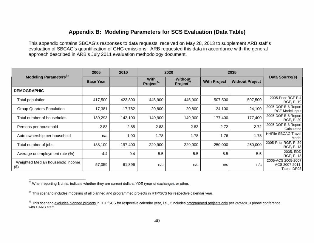
40

Appendix B: Modeling Parameters for SCS Evaluation (Data Table) This appendix contains SBCAG’s responses to data requests, received on May 28, 2013 to supplement ARB staff’s evaluation of SBCAG’s quantification of GHG emissions. ARB requested this data in accordance with the general approach described in ARB’s July 2011 evaluation methodology document.

Modeling Parameters 23 2005 2010 2020 2035

Data Source(s) Base Year With

Project 24 Without Project 25 With Project Without Project

DEMOGRAPHIC

Total population 417,500 423,800 445,900 445,900 507,500 507,500 2005-Prior RGF P.4 RGF, P. 19

Group Quarters Population 17,381 17,782 20,800 20,800 24,100 24,100 2005-DOF E-8 Report RGF Model input

Total number of households 139,293 142,100 149,900 149,900 177,400 177,400 2005-DOF E-8 Report RGF, P. 20

Persons per household 2.83 2.85 2.83 2.83 2.72 2.72 2005-DOF E-8 Report Calculated

Auto ownership per household n/a 1.90 1.78 1.78 1.76 1.78 HHFile SBCAG Travel Model

Total number of jobs 188,100 197,400 229,900 229,900 250,000 250,000 2005-Prior RGF, P. 39 RGF, P. 13

Average unemployment rate (%) 4.4 9.4 5.5 5.5 5.5 5.5 2005, EDD RGF, P. 18

Weighted Median household income ($) 57,059 61,896 n/c n/c n/c n/c

2005-ACS 2005-2007 ACS 2007-2011,

Table, DP03

23 When reporting $ units, indicate whether they are current dollars, YOE (year of exchange), or other.

24 This scenario includes modeling of all planned and programmed projects in RTP/SCS for respective calendar year.

25 This scenario excludes planned projects in RTP/SCS for respective calendar year, i.e., it includes programmed projects only per 2/25/2013 phone conference with CARB staff.

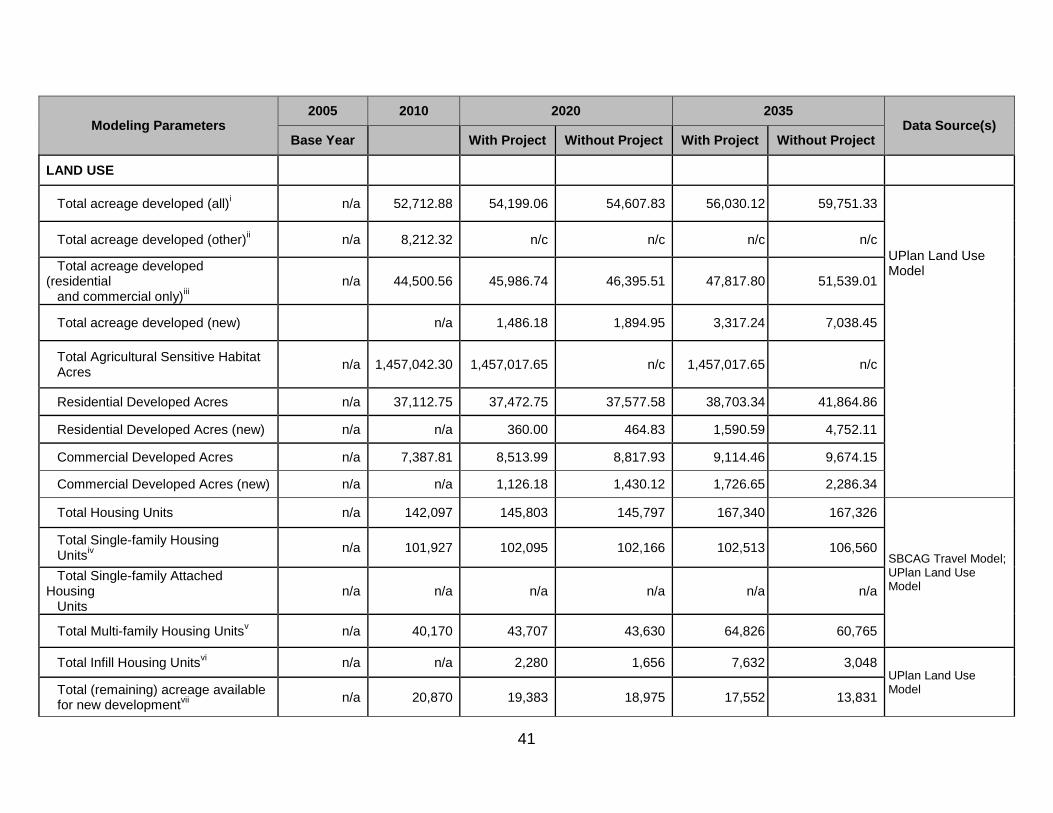
41

Modeling Parameters 2005 2010 2020 2035

Data Source(s) Base Year With Project Without Project With Project Without Project

LAND USE

Total acreage developed (all)i n/a 52,712.88 54,199.06 54,607.83 56,030.12 59,751.33

UPlan Land Use Model

Total acreage developed (other)ii n/a 8,212.32 n/c n/c n/c n/c

Total acreage developed (residential and commercial only)iii

n/a 44,500.56 45,986.74 46,395.51 47,817.80 51,539.01

Total acreage developed (new) n/a 1,486.18 1,894.95 3,317.24 7,038.45

Total Agricultural Sensitive Habitat Acres

n/a 1,457,042.30 1,457,017.65 n/c 1,457,017.65 n/c

Residential Developed Acres n/a 37,112.75 37,472.75 37,577.58 38,703.34 41,864.86

Residential Developed Acres (new) n/a n/a 360.00 464.83 1,590.59 4,752.11

Commercial Developed Acres n/a 7,387.81 8,513.99 8,817.93 9,114.46 9,674.15

Commercial Developed Acres (new) n/a n/a 1,126.18 1,430.12 1,726.65 2,286.34

Total Housing Units n/a 142,097 145,803 145,797 167,340 167,326

SBCAG Travel Model; UPlan Land Use Model

Total Single-family Housing Unitsiv

n/a 101,927 102,095 102,166 102,513 106,560

Total Single-family Attached Housing Units

n/a n/a n/a n/a n/a n/a

Total Multi-family Housing Unitsv n/a 40,170 43,707 43,630 64,826 60,765

Total Infill Housing Unitsvi n/a n/a 2,280 1,656 7,632 3,048 UPlan Land Use Model Total (remaining) acreage available

for new developmentvii n/a 20,870 19,383 18,975 17,552 13,831

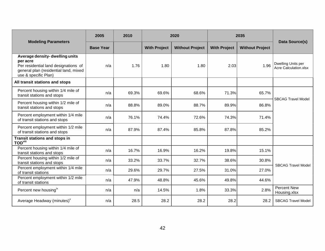
42

Modeling Parameters 2005 2010 2020 2035

Data Source(s) Base Year With Project Without Project With Project Without Project

Average density - dwelling units

per acre Per residential land designations of general plan (residential land, mixed use & specific Plan)

n/a 1.76 1.80 1.80 2.03 1.96 Dwelling Units per Acre Calculation.xlsx

All transit stations and stops

Percent housing within 1/4 mile of transit stations and stops

n/a 69.3% 69.6% 68.6% 71.3% 65.7%

SBCAG Travel Model Percent housing within 1/2 mile of transit stations and stops n/a 88.8% 89.0% 88.7% 89.9% 86.8%

Percent employment within 1/4 mile of transit stations and stops

n/a 76.1% 74.4% 72.6% 74.3% 71.4%

Percent employment within 1/2 mile of transit stations and stops

n/a 87.9% 87.4% 85.8% 87.8% 85.2%

Transit stations and stops in TODviii

Percent housing within 1/4 mile of transit stations and stops n/a 16.7% 16.9% 16.2% 19.8% 15.1%

SBCAG Travel Model

Percent housing within 1/2 mile of transit stations and stops

n/a 33.2% 33.7% 32.7% 38.6% 30.8%

Percent employment within 1/4 mile of transit stations

n/a 29.6% 29.7% 27.5% 31.0% 27.0%

Percent employment within 1/2 mile of transit stations

n/a 47.9% 48.8% 45.6% 49.8% 44.6%

Percent new housingix n/a n/a 14.5% 1.8% 33.3% 2.8% Percent New Housing.xlsx

Average Headway (minutes)x n/a 28.5 28.2 28.2 28.2 28.2 SBCAG Travel Model

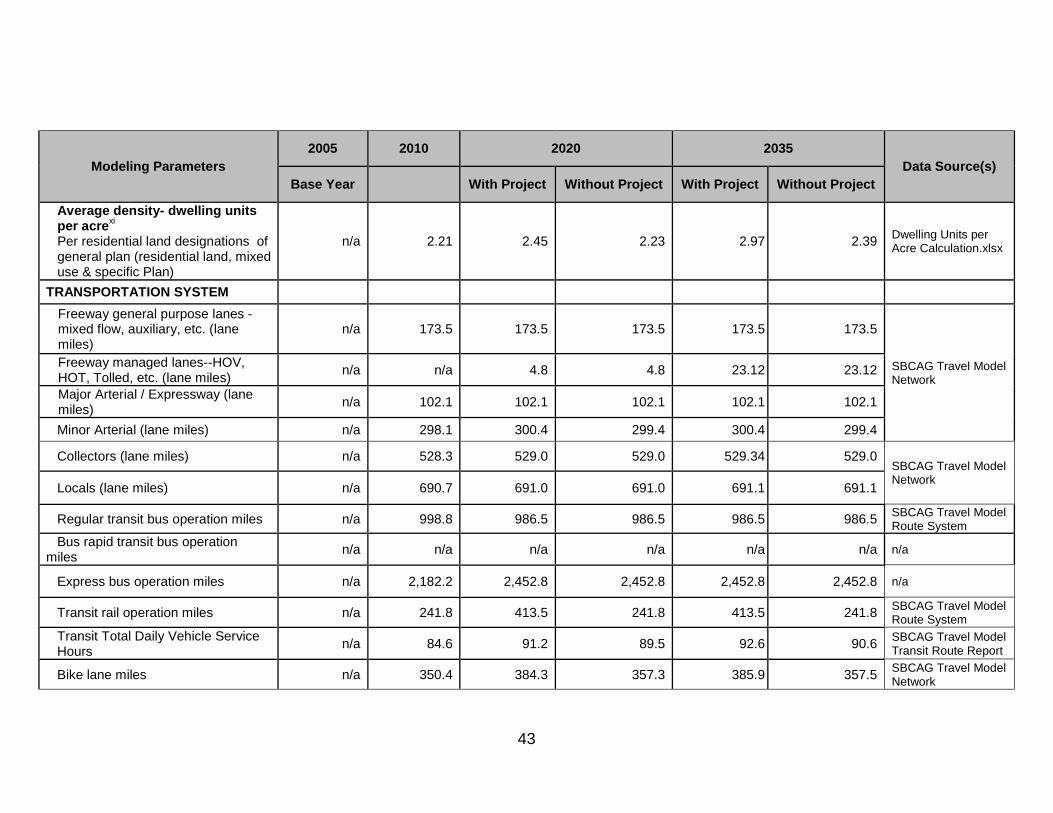
43

Modeling Parameters 2005 2010 2020 2035

Data Source(s) Base Year With Project Without Project With Project Without Project

Average density - dwelling units per acre xi Per residential land designations of general plan (residential land, mixed use & specific Plan)

n/a 2.21 2.45 2.23 2.97 2.39 Dwelling Units per Acre Calculation.xlsx

TRANSPORTATION SYSTEM

Freeway general purpose lanes - mixed flow, auxiliary, etc. (lane miles)

n/a 173.5 173.5 173.5 173.5 173.5

SBCAG Travel Model Network

Freeway managed lanes--HOV, HOT, Tolled, etc. (lane miles)

n/a n/a 4.8 4.8 23.12 23.12

Major Arterial / Expressway (lane miles)

n/a 102.1 102.1 102.1 102.1 102.1

Minor Arterial (lane miles) n/a 298.1 300.4 299.4 300.4 299.4

Collectors (lane miles) n/a 528.3 529.0 529.0 529.34 529.0 SBCAG Travel Model Network

Locals (lane miles) n/a 690.7 691.0 691.0 691.1 691.1

Regular transit bus operation miles n/a 998.8 986.5 986.5 986.5 986.5 SBCAG Travel Model Route System

Bus rapid transit bus operation miles

n/a n/a n/a n/a n/a n/a n/a

Express bus operation miles n/a 2,182.2 2,452.8 2,452.8 2,452.8 2,452.8 n/a

Transit rail operation miles n/a 241.8 413.5 241.8 413.5 241.8 SBCAG Travel Model Route System

Transit Total Daily Vehicle Service Hours

n/a 84.6 91.2 89.5 92.6 90.6 SBCAG Travel Model Transit Route Report

Bike lane miles n/a 350.4 384.3 357.3 385.9 357.5 SBCAG Travel Model Network

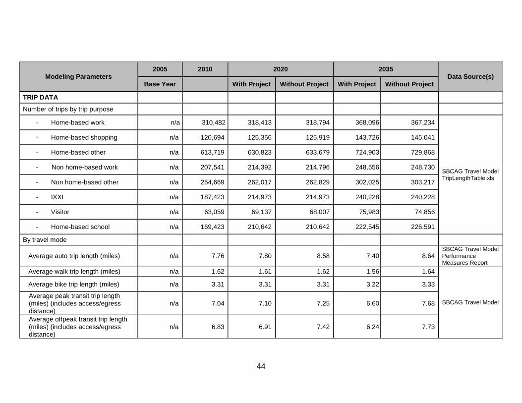
44

Modeling Parameters 2005 2010 2020 2035

Data Source(s) Base Year With Project Without Project With Project Without Project

TRIP DATA

Number of trips by trip purpose

- Home-based work n/a 310,482 318,413 318,794 368,096 367,234

SBCAG Travel Model TripLengthTable.xls

- Home-based shopping n/a 120,694 125,356 125,919 143,726 145,041

- Home-based other n/a 613,719 630,823 633,679 724,903 729,868

- Non home-based work n/a 207,541 214,392 214,796 248,556 248,730

- Non home-based other n/a 254,669 262,017 262,829 302,025 303,217

- IXXI n/a 187,423 214,973 214,973 240,228 240,228

- Visitor n/a 63,059 69,137 68,007 75,983 74,856

- Home-based school n/a 169,423 210,642 210,642 222,545 226,591

By travel mode

Average auto trip length (miles) n/a 7.76 7.80 8.58 7.40 8.64 SBCAG Travel Model Performance Measures Report

Average walk trip length (miles) n/a 1.62 1.61 1.62 1.56 1.64

SBCAG Travel Model

Average bike trip length (miles) n/a 3.31 3.31 3.31 3.22 3.33

Average peak transit trip length (miles) (includes access/egress distance)

n/a 7.04 7.10 7.25 6.60 7.68

Average offpeak transit trip length (miles) (includes access/egress distance)

n/a 6.83 6.91 7.42 6.24 7.73

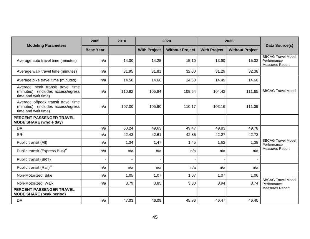
45

Modeling Parameters 2005 2010 2020 2035

Data Source(s) Base Year With Project Without Project With Project Without Project

Average auto travel time (minutes) n/a 14.00 14.25 15.10 13.90 15.32 SBCAG Travel Model Performance Measures Report

Average walk travel time (minutes) n/a 31.95 31.81 32.00 31.29 32.38

SBCAG Travel Model

Average bike travel time (minutes) n/a 14.50 14.66 14.60 14.49 14.60

Average peak transit travel time (minutes) (includes access/egress time and wait time)

n/a 110.92 105.84 109.54 104.42 111.65

Average offpeak transit travel time (minutes) (includes access/egress time and wait time)

n/a 107.00 105.90 110.17 103.16 111.39

PERCENT PASSENGER TRAVEL MODE SHARE (whole day)

DA n/a 50.24 49.63 49.47 49.83 49.78

SBCAG Travel Model Performance Measures Report

SR n/a 42.43 42.61 42.85 42.27 42.73

Public transit (All) n/a 1.34 1.47 1.45 1.62 1.38

Public transit (Express Bus)xii n/a n/a n/a n/a n/a n/a

Public transit (BRT) - -- - - - -

Public transit (Rail)xii n/a n/a n/a n/a n/a n/a

SBCAG Travel Model Performance Measures Report

Non-Motorized: Bike n/a 1.05 1.07 1.07 1.07 1.06

Non-Motorized: Walk n/a 3.79 3.85 3.80 3.94 3.74

PERCENT PASSENGER TRAVEL MODE SHARE (peak period)

DA n/a 47.03 46.09 45.96 46.47 46.40

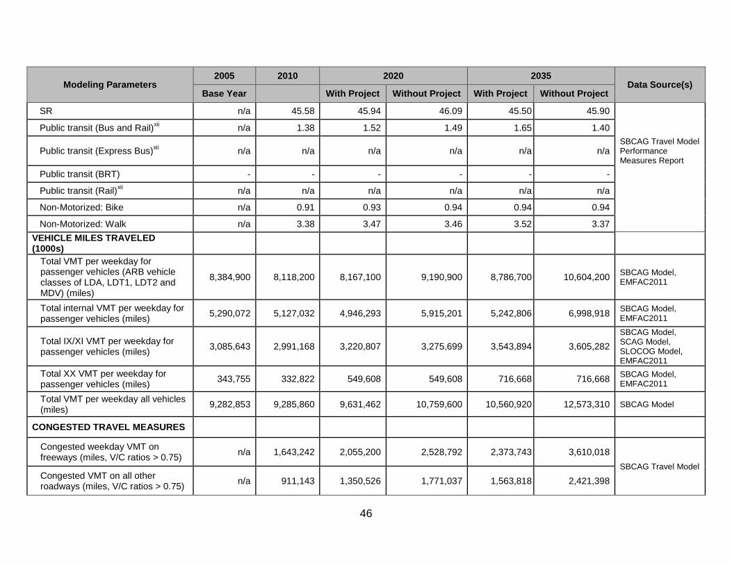
46

Modeling Parameters 2005 2010 2020 2035

Data Source(s) Base Year With Project Without Project With Project Without Project

SR n/a 45.58 45.94 46.09 45.50 45.90

Public transit (Bus and Rail)xii n/a 1.38 1.52 1.49 1.65 1.40

Public transit (Express Bus)xii n/a n/a n/a n/a n/a n/a SBCAG Travel Model Performance Measures Report

Public transit (BRT) - - - - - -

Public transit (Rail)xii n/a n/a n/a n/a n/a n/a

Non-Motorized: Bike n/a 0.91 0.93 0.94 0.94 0.94

Non-Motorized: Walk n/a 3.38 3.47 3.46 3.52 3.37

VEHICLE MILES TRAVELED (1000s)

Total VMT per weekday for passenger vehicles (ARB vehicle classes of LDA, LDT1, LDT2 and MDV) (miles)

8,384,900 8,118,200 8,167,100 9,190,900 8,786,700 10,604,200 SBCAG Model, EMFAC2011

Total internal VMT per weekday for passenger vehicles (miles)

5,290,072 5,127,032 4,946,293 5,915,201 5,242,806 6,998,918 SBCAG Model, EMFAC2011

Total IX/XI VMT per weekday for passenger vehicles (miles)

3,085,643 2,991,168 3,220,807 3,275,699 3,543,894 3,605,282

SBCAG Model, SCAG Model, SLOCOG Model, EMFAC2011

Total XX VMT per weekday for passenger vehicles (miles)

343,755 332,822 549,608 549,608 716,668 716,668 SBCAG Model, EMFAC2011

Total VMT per weekday all vehicles (miles)

9,282,853 9,285,860 9,631,462 10,759,600 10,560,920 12,573,310 SBCAG Model

CONGESTED TRAVEL MEASURES

Congested weekday VMT on freeways (miles, V/C ratios > 0.75)

n/a 1,643,242 2,055,200 2,528,792 2,373,743 3,610,018

SBCAG Travel Model Congested VMT on all other roadways (miles, V/C ratios > 0.75)

n/a 911,143 1,350,526 1,771,037 1,563,818 2,421,398

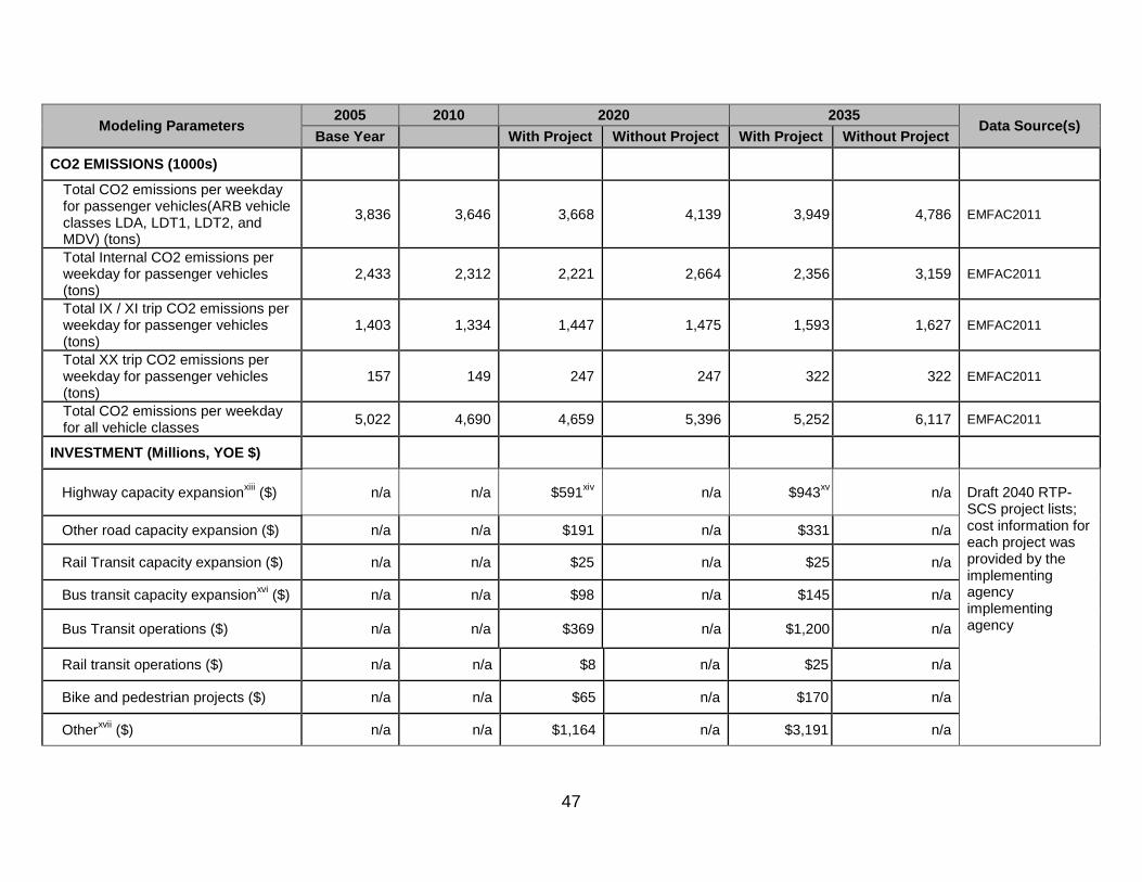
47

Modeling Parameters 2005 2010 2020 2035

Data Source(s) Base Year With Project Without Project With Project Without Project

CO2 EMISSIONS (1000s)

Total CO2 emissions per weekday for passenger vehicles(ARB vehicle classes LDA, LDT1, LDT2, and MDV) (tons)

3,836 3,646 3,668 4,139 3,949 4,786 EMFAC2011

Total Internal CO2 emissions per weekday for passenger vehicles (tons)

2,433 2,312 2,221 2,664 2,356 3,159 EMFAC2011

Total IX / XI trip CO2 emissions per weekday for passenger vehicles (tons)

1,403 1,334 1,447 1,475 1,593 1,627 EMFAC2011

Total XX trip CO2 emissions per weekday for passenger vehicles (tons)

157 149 247 247 322 322 EMFAC2011

Total CO2 emissions per weekday for all vehicle classes

5,022 4,690 4,659 5,396 5,252 6,117 EMFAC2011

INVESTMENT (Millions, YOE $)

Highway capacity expansionxiii ($) n/a n/a $591xiv n/a $943xv n/a Draft 2040 RTP-SCS project lists; cost information for each project was provided by the implementing agency implementing agency

Other road capacity expansion ($) n/a n/a $191 n/a $331 n/a

Rail Transit capacity expansion ($) n/a n/a $25 n/a $25 n/a

Bus transit capacity expansionxvi ($) n/a n/a $98 n/a $145 n/a

Bus Transit operations ($) n/a n/a $369 n/a $1,200 n/a

Rail transit operations ($) n/a n/a $8 n/a $25 n/a

Bike and pedestrian projects ($) n/a n/a $65 n/a $170 n/a

Otherxvii ($) n/a n/a $1,164 n/a $3,191 n/a

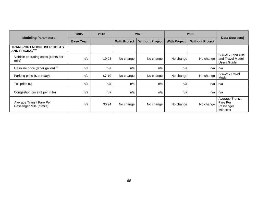
48

Modeling Parameters 2005 2010 2020 2035

Data Source(s) Base Year With Project Without Project With Project Without Project

TRANSPORTATION USER COSTS AND PRICINGxviii

Vehicle operating costs (cents per mile)

n/a 19.93 No change No change No change No change SBCAG Land Use and Travel Model Users Guide

Gasoline price ($ per gallon)xix n/a n/a n/a n/a n/a n/a n/a

Parking price ($ per day) n/a $7-10 No change No change No change No change SBCAG Travel Model

Toll price ($) n/a n/a n/a n/a n/a n/a n/a

Congestion price ($ per mile) n/a n/a n/a n/a n/a n/a n/a

Average Transit Fare Per Passenger Mile (¢/mile) n/a $0.24 No change No change No change No change

Average Transit Fare Per Passenger Mile.xlsx

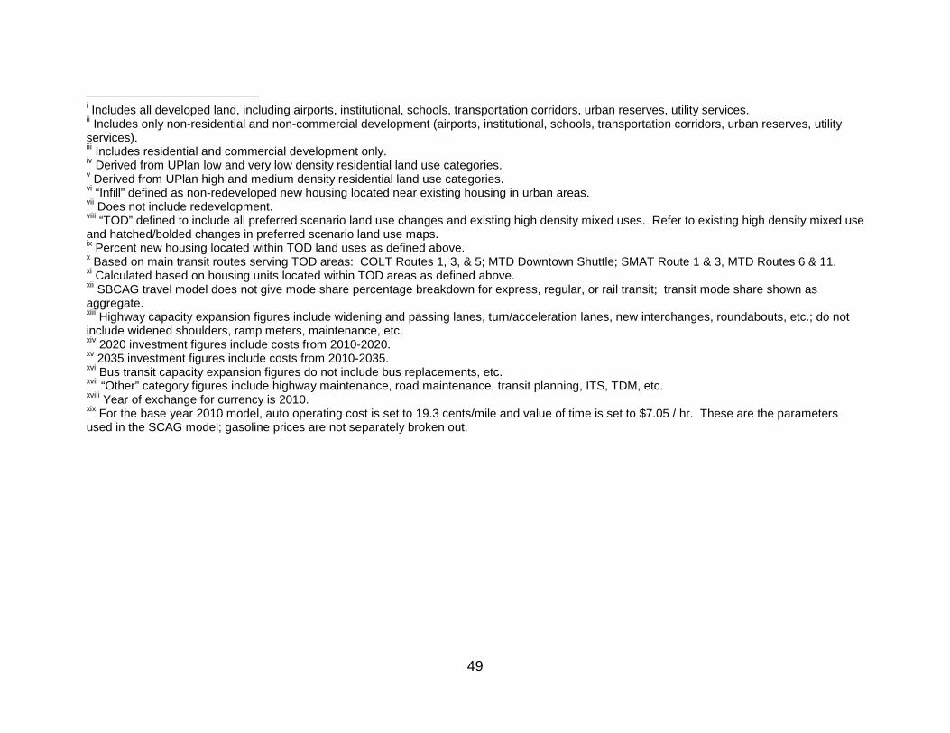
49

i Includes all developed land, including airports, institutional, schools, transportation corridors, urban reserves, utility services. ii Includes only non-residential and non-commercial development (airports, institutional, schools, transportation corridors, urban reserves, utility services). iii Includes residential and commercial development only. iv Derived from UPlan low and very low density residential land use categories. v Derived from UPlan high and medium density residential land use categories. vi “Infill” defined as non-redeveloped new housing located near existing housing in urban areas. vii Does not include redevelopment. viii “TOD” defined to include all preferred scenario land use changes and existing high density mixed uses. Refer to existing high density mixed use and hatched/bolded changes in preferred scenario land use maps. ix Percent new housing located within TOD land uses as defined above. x Based on main transit routes serving TOD areas: COLT Routes 1, 3, & 5; MTD Downtown Shuttle; SMAT Route 1 & 3, MTD Routes 6 & 11. xi Calculated based on housing units located within TOD areas as defined above. xii SBCAG travel model does not give mode share percentage breakdown for express, regular, or rail transit; transit mode share shown as aggregate. xiii Highway capacity expansion figures include widening and passing lanes, turn/acceleration lanes, new interchanges, roundabouts, etc.; do not include widened shoulders, ramp meters, maintenance, etc. xiv 2020 investment figures include costs from 2010-2020. xv 2035 investment figures include costs from 2010-2035. xvi Bus transit capacity expansion figures do not include bus replacements, etc. xvii “Other” category figures include highway maintenance, road maintenance, transit planning, ITS, TDM, etc. xviii Year of exchange for currency is 2010. xix For the base year 2010 model, auto operating cost is set to 19.3 cents/mile and value of time is set to $7.05 / hr. These are the parameters used in the SCAG model; gasoline prices are not separately broken out.