Quantification and controls of wetland greenhouse gas

Quantification and controls of wetland greenhouse gas emissions

by

Gavin McNicol

A dissertation submitted in partial satisfaction of the

requirements for the degree of

Doctor of Philosophy

in

Environmental Science, Policy, and Management

in the

Graduate Division

of the

University of California, Berkeley

Committee in charge:

Professor Whendee L. Silver, Chair Professor Dennis D. Baldocchi

Professor John D. Coates

Summer 2016


© 2016

by Gavin McNicol

1

Abstract


by

Gavin McNicol

Doctor of Philosophy in Environmental Science, Policy, and Management

University of California, Berkeley

Professor Whendee L. Silver, Chair Wetlands cover only a small fraction of the Earth’s land surface, but have a disproportionately large influence on global climate. Low oxygen conditions in wetland soils slows down decomposition, leading to net carbon dioxide sequestration over long timescales, while also favoring the production of redox sensitive gases such as nitrous oxide and methane. Freshwater marshes in particular sustain large exchanges of greenhouse gases under temperate or tropical climates and favorable nutrient regimes, yet have rarely been studied, leading to poor constraints on the magnitude of marsh gas sources, and the biogeochemical drivers of flux variability. The Sacramento-San Joaquin Delta in California was once a great expanse of tidal and freshwater marshes but underwent drainage for agriculture during the last two centuries. The resulting landscape is unsustainable with extreme rates of land subsidence and oxidation of peat soils lowering the surface elevation of much of the Delta below sea level. Wetland restoration has been proposed as a means to slow further subsidence and rebuild peat however the balance of greenhouse gas exchange in these novel ecosystems is still poorly described. In this dissertation I first explore oxygen availability as a control on the composition and magnitude of greenhouse gas emissions from drained wetland soils. In two separate experiments I quantify both the temporal dynamics of greenhouse gas emission and the kinetic sensitivity of gas production to a wide range of oxygen concentrations. This work demonstrated the very high sensitivity of carbon dioxide, methane, and nitrous oxide production to oxygen availability, in carbon rich wetland soils. I also found the temporal dynamics of gas production to follow a sequence predicted by thermodynamics and observed spatially in other soil or sediment systems. In the latter part of my dissertation I conduct two field studies to quantify greenhouse gas exchange and understand the carbon sources for decomposition in a 1 km2 restored wetland in the Sacramento Delta. By coupling flux measurements at multiple-scales with remote sensing imagery I showed that large methane emissions produce an overall climate warming effect from the wetland for the next several centuries, despite relatively high productivity. I also used radiocarbon analyses of wetland sediment carbon dioxide and methane to show that both bulk peat and recently fixed carbon contribute to decomposition in the wetland, and that their relative importance is regulated by proximity to, and the phenological cycles of, emergent vegetation.

i

For my parents

ii

Table of Contents

Chapter 1: Introduction……………………………………………………………....... 1

Chapter 2: Separate effects of flooding and anaerobiosis on soil greenhouse gas emissions and redox sensitive biogeochemistry………………………………………………….. 7

Chapter 3: Non-linear response of carbon dioxide and methane emissions to oxygen availability in a drained Histosol...……………………………………………………. 24

Chapter 4: Beyond the methanogenic black-box: Effects of seasonality, transport pathway, and spatial structure on wetland greenhouse gas emissions….……………………... 36

Chapter 5: Radiocarbon reveals dynamic contributions from recent photosynthesis and bulk peat carbon to decomposition in a restored wetland…………..……………..... 68

iii

Acknowledgements

‘Life is an aggregate, an aggregate of all the lives that have ever been lived on the planet Earth.’

-Martin Amis, Money [1984]

A network of mentors, teachers, colleagues, friends, and family carved out the path of my graduate school journey. Over the last eight years, this network - my personal ecology - has trained me how to think, how to write, how to do science, and also taught me many lessons in how to live. I cannot possibly be exhaustive in acknowledging all the support I have benefitted from but I will do my best to highlight those most indispensible contributions.

I am particularly grateful to Professor Whendee Silver, my Ph.D. advisor, whose

unwavering commitment to my success saved me from the innumerable pitfalls of graduate study. Whendee first inspired me as an engaging ecosystem ecology teacher who planted the seed of pursuing a research career, and then, during my early graduate career, as an innovative and tireless ecologist whose uniquely potent blend of scientific pragmatism and idealism nurtured significant shifts in my perception of the traditional dichotomy of pure and applied sciences. In other words, Whendee made me into a lifelong ecologist.

I must also thank Professor Dennis Baldocchi whose advice to think from first principles

and make connections between biology and physics has provided me an intellectual toolset to tackle all the ecological questions in my research. I am especially grateful to him for introducing me to Schrödinger’s What is Life? Other formative academic mentors were Professor Gary Sposito and Professor John Coates, who taught me about redox, and Professor Todd Dawson and Dr. Paul Brooks, who helped me learn the fundamentals of isotope analysis and its applications. I also would never have seriously considered international graduate study were it not for the encouragement of Professor Iryna Dronova.

I must also thank the technicians, graduate students, and post-doctoral scholars of the

Silver lab. I would not have survived graduate school without the help of Wendy Yang, who put me through lab boot camp in my first summer and was patient with my technical questions. Rebecca Ryals and Steven Hall were always eager to help me, often quickly dispelling my stress over what I thought to be vexing or intractable research problems. They remain two of the most principled and committed ecologists I have met, and I could not have had better graduate student role models. Heather Dang accompanied me on the majority of my Delta field trips; more than halving the challenge involved. Other Silver lab support I am grateful for came from Summer Ahmed, Maya Almarez, Tyler Anthony, Jackson Chin, Marcia DeLonge, Omar Gutièrrez del Arroyo, Luke Lintott, Daniel Liptzin, Allegra Mayer, Andrew McDowell, Andrew Moyes, Christine O’Connell, Justine Owen, Ryan Salladay, Laura Southworth, Jonathan Treffkorn, Michelle Wong, Tana Wood, and Sintana Vergara.

I had the privilege of a working with a diverse and committed group of researchers at

Lawrence Livermore National Laboratory. I must thank Brian LaFranchi who patiently supported me during three years of methane extractions. I am also grateful for the thoughtful supervision of Tom Guilderson, Karis McFarlane, and Katherine Heckmann, who gave me the

iv

freedom to explore and learn from my own mistakes in a unique laboratory setting but who were present and helpful whenever I needed it. Caroline Herman, Paula Zermeno, and Alexandra Hedgpeth repeatedly helped me in the graphite lab and Nanette Sorensen guided me past the teeth of The Leviathan. I also enjoyed the support and camaraderie of Jennifer Pett-Ridge and Ate Visser. Last, but certainly not least, Rebecca (Skye) Bosworth who offered me friendship at a critical time.

I am also thankful for the personal support I received during my six years at Berkeley.

My greatest privilege is that I am my parents’ son. My mother never lets me be anything other than my best, and my father gives me the freedom to be whoever that means I have to be. I cannot thank them enough for selflessly indulging my American dreams. I must also thank my sister Kathryn who balanced my transatlanticism in every sense, and my grandmothers, Joan and Cathy, who regularly traversed it with their letters. A second family welcomed me when I first arrived in the United States, the DiStefano’s of Orinda: Drew, Susan, Tony, and Ted. Their generosity left a lasting impression on me and I think they represent some of America’s finest. Others who left indelible marks on my life are Joey Lam, Christopher Goetz, Jose Manuel Diaz-Oldenburg, Virgilio Tinio, Corey Lons, Jorge Santiago-Ortiz, Eric Phelan, Derek Tam-Scott, Chandra Brouch, Talon Clayton, Jason Yan, and Jon Gonzalez. I thank them for their patience and love as I navigated the divide between two very different worlds.

I want to acknowledge the support of peers and staff of the UC Berkeley Department of

Environmental Science, Policy, and Management. I must thank my fellow Berkeley graduate students Sara Knox, Kari Finstad, Sydney Glassman, Matteo Kausch, David Rolfe, Luke Macaulay, Lauren Hallett, and Maddie Girard for their close friendship. Judy Smithson and Roxanne Heglar easily unraveled even my best attempts to concoct wicked administrative problems. Finally, portions of this dissertation have been reprinted, with permission, from the Journal of Geophysical Research: Biogeosciences and Biogeochemistry, and I thank the Wiley and Springer publishing companies for that permission.

1

Chapter 1: Introduction

“Years ago I used to worry about the degree to which I had specialized… my studies involved only the rods and cones of the retina, and in them only the visual pigments. A sadly limited

peripheral business, fit for escapists. But it is as though this were a very narrow window through which at a distance one can see only a crack of light. As one comes closer the view grows wider

and wider, until finally through this same narrow window one is looking at the universe.’ - George Wald,“Life and Light” [1959]

Wetlands globally span a broad range of environmental conditions; across gradients in

climate, soil type, hydrology, and nutrient and oxygen (redox) regimes, and, as a result, they play host to a great variety of plant and microbial life (Mitsch and Gosselink, 2015). A gradient in productivity can be delineated from the rain-fed, nutrient poor peatbogs of high latitudes, such as those of the northern British Isles, Siberia, Scandinavia, Canada, and Patagonia, through moderately productive and temporarily inundated fens found often in riparian zones, and last into permanently flooded, groundwater-fed marshes whose adapted emergent vegetation supports extremely high rates of carbon uptake and release in warmer Mediterranean and tropical climates (Bridgham et al. 2013).

Flooded soils in these varied wetland ecosystems globally have a significant influence on

the climate system via the biosphere-atmosphere exchange of climate forcing trace gases, otherwise known as greenhouse gases (IPCC, 2013; Neubauer, 2015). Over long time scales, wetlands have cooling effects on climate via their uptake of carbon dioxide (CO2). This occurs as oxygen (O2) depletion in wetland soil slows decomposition (Freeman et al. 2001), which, as a result, tends to be outpaced by primary productivity (Limpens et al. 2008). Over the course of the Holocene, or longer time periods at low latitudes, wetlands have sequestered approximately 1,000 Pg C-CO2 – representing almost one-third of the global soil carbon reservoir – and thus have had a long-term cooling effect on the Earth’s climate system by removing CO2 from the atmosphere (Limpens et al. 2008).

Running counter to CO2 uptake, are potential warming effects of two other greenhouse

gas fluxes, namely methane (CH4) and nitrous oxide (N2O) emission (Conrad, 1996). The microbial production and consumption of these gases is highly sensitive to O2 – or redox – conditions and thus forces an intrinsic trade off to the benefit of CO2 sequestration. Globally, wetlands are the largest non-anthropogenic source of atmospheric CH4, accounting for approximately 30% of ‘natural’ emissions – or approximately 200-300 Mt C-CH4 emissions per year (IPCC, 2013). Freshwater marshes in warmer climates are particularly intense sources of CH4, though have been studied far less than CH4 exchange in expansive high-latitude peatlands (Bridgham et al. 2013). Nitrous oxide has been studied even less (Schlesinger 2013; Neubauer and Megonigal, 2015), but some recent studies suggest wetlands may function as dynamic sources and sinks of this very potent greenhouse gas and that production of N2O in wetlands is non-linearly sensitive to O2 availability (Venkiteswaran et al. 2014; Beauleiu et al. 2015; Helton et al. 2015), making it both an indicator of ecosystem redox status as well as a contributor to the overall greenhouse gas budget.

2

To fully understand wetland gas exchange effects on climate the emissions must be integrated over a certain period of time. Though methane and nitrous oxide are commonly reported to have a warming potential 45 and 270 times that of CO2, this is strictly over a 100-year time horizon (IPCC, 2013). These conversions are useful for establishing a climate effect from emissions inventories at a snapshot in time, but more general patterns can be described. The cooling effects of CO2 uptake tend to accumulate over time, as sequestration can last centuries to millennia, whereas the short atmospheric lifetime of CH4 (~12 years) means warming effects from CH4 tend to asymptote and will be overwhelmed by CO2 sequestration over decades to centuries (Neubauer and Megonigal, 2015).

In my dissertation I have investigated rates and controls of greenhouse gas exchange in

the drained and restored wetlands of the Sacramento Delta (Delta, hereafter) California. Some of the greatest extents of wetlands globally exist in the major river delta of the world (Zedler and Kercher, 2005), and the Delta at the confluence of the San Joaquin and Sacramento Rivers in California is no exception to that pattern. Though the contemporary Delta is almost entirely (> 90%) leveed and drained for agriculture and human settlement, the Delta of the pre-Industrial Holocene was a >2,000 km2 region of tidal and freshwater emergent marshes (Whipple et al. 2012). These marshes were also peat forming and, high rates of primary production coupled to alluvial sedimentation, meant that peat accumulation kept pace with sea-level rise during the last 8,000 years – building 5 to 20 m of organic C-rich soils (Drexler et al. 2009a). Since drainage began in the late 19th century, the Delta landscape has been markedly changed with clearly defined island boundaries replacing the former shifting ecological transitions of water and marsh (Whipple et al. 2012). The interior of most of the Delta islands now lie several meters below sea-level due to extreme rates of soil subsidence – both physical compaction and secondary oxidation of organic C – threatening the region with inundation, and the greater California population with salt-intrusion of it’s water supplies (Drexler et al. 2009b). As a result of the unsustainability of business-as-usual land management in the Delta, pressure is mounting to restore wetlands in the region with managed re-flooding (Miller et al. 2000). However, significant wetland restoration in the Delta will again change the dynamics of greenhouse gas exchange, likely substituting the large CO2 source from aerobic microbial oxidation of peat for a CO2 sink (Hatala et al. 2012; Knox et al. 2015) and greater production of redox-sensitive gases such as CH4 and N2O.

In chapter two of my dissertation I explored the physical and chemical effects of flooding

on wetland soil biogeochemistry and greenhouse gas dynamics. I used controlled flooding and anoxic headspace treatments to distinguish the quantitative role of O2-based metabolism in regulating soil CO2, CH4 and N2O production, but also explored other physical effects of flooding, such as increases solute mobilization, on gas exchange. By following soil greenhouse gas dynamics over time I found respiration rates were highly sensitive to O2 in a drained peatland Histosol collected from the Delta, and that greenhouse gas dynamics overall followed a predictable thermodynamic sequence often observed spatially in soils, sediments, and groundwater (Takai and Kamura 1966; Peters and Conrad, 1996). These results suggested that the complexity of gas release in flooded wetland, or low-redox status, soils could be broadly distilled to predictable patterns related to the persistence of O2 depletion.

Given the high O2-sensitivity of Delta Histosol greenhouse gas exchange observed in my

first experiments, in chapter three I asked the question: what is functionally low gas-phase O2

3

from a soil biogeochemical perspective? Much of the contemporary geochemical literature assumes that low O2 conditions (anoxic soil) occurs at O2 concentrations below 1% (Berner 1981; Scott and Morgan 1990; Chapelle et al. 1995), yet O2 availability would still be in great excess of other trace gas reactants such as CH4 at this apparent anoxic threshold. I therefore varied O2 concentrations over several orders of magnitude (0.03 – 20%) to explore potential non-linearity between CH4 and CO2 emission, and O2 concentration in the same drained Delta Histosol. I found a non-linear, highly sensitive, relationship between soil CO2 and CH4 flux, and O2 availability, suggesting that linear interpolation of process rates from percent-range concentrations of O2 could be highly misleading.

In the last two chapters of my dissertation I shifted focus from experimental

manipulations of the drained, O2-exposed peatlands of the Delta to in situ observations from a newly restored emergent wetland. Marsh ecosystems feature spatial heterogeneity in canopy height, plant species, and soil drainage that present challenges to estimating and scaling trace gas exchange (Bridgham et al. 2013; Sturtevant et al. 2015). Combing flux measurements at different scales is a promising methodological approach that I developed and applied in chapter four. Specifically, I combined spatially explicit chamber measurements with continuous, field-scale, eddy-covariance observations to estimate wetland greenhouse gas fluxes of CO2, CH4, and N2O. The approach permitted quantitative partitioning of gas fluxes – and their associated radiative forcing effects - between open-water pools and vegetated zones. One key finding was that zones of emergent vegetation accounted for >90% of wetland CH4 emissions, while the overall radiative forcing effect of greenhouse gas emissions was larger for open-water zones, due to high rates CO2 emission. A second important outcome of the study was that the highest N2O fluxes occurred during the colder winter months. These data support a recent paradigm shift away from simple temperature response functions for gas flux predictions (Davidson and Janssens, 2006; Oikawa et al. 2014) that are often used for CO2 and CH4. Instead, the asynchronous fluxes of O2-sensitive CH4 and N2O gases suggest seasonal wetland redox oscillations can be important in regulating the composition of wetland greenhouse gas emissions.

Vegetation plays a central role in ecosystem gas exchange. In wetlands, emergent plants

typically dominate autotrophic CO2 uptake (Mitsch et al. 2012), while they also act as a conduit and substrate source for CH4 release (Laanbroek, 2010). The net radiative forcing effect of these opposing fluxes is still highly uncertain, as is the respective contributions of recently fixed C versus bulk peat C in wetland decomposition. In chapter five, I developed the capability for 14C isotope analysis of CH4. I used 14C to distinguish the C substrate sources for wetland CH4

production, and related spatial and temporal variability to emergent plant presence and activity. My approach exploited the large contrast in isotopic composition of bulk wetland organic matter with atmospheric CO2 used for present photosynthesis, which is a legacy of drainage at the Delta wetland site (Drexler et al. 2009b). I collected samples from the sediment bubble inventory in open-water and vegetated zones, as well as gas from plant-stems, over one year. I tested and utilized a new vacuum line for the cryogenic isolation of CH4 from mixed air samples for AMS 14C analysis (Petrenko et al. 2008). The results demonstrated that seasonality in autotrophic productivity and temperature drives wetland C dynamics and, using an isotopic mixing model, I found that proximity to emergent vegetation stimulated CH4 production from recently fixed C sources, and that this effect varied seasonally with cycles of plant phenology.

4

References Beaulieu JJ, Nietch CT, Young JL (2015) Controls on nitrous oxide production and consumption in reservoirs of the Ohio River Basin. Journal of Geophysical Research: Biogeosciences, 120, 1995-2010. Berner RA (1981) A new geochemical classification of sedimentary environments. Journal of Sedimentary Research, 51, 359-365. Bridgham SD, Cadillo-Quiroz H, Keller JK, Zhuang Q (2013) Methane emissions from wetlands: biogeochemical, microbial, and modeling perspectives from local to global scales. Glob Chang Biol, 19, 1325-1346. Chapelle FH, Mcmahon PB, Dubrovsky NM, Fujii RF, Oaksford ET, Vroblesky DA (1995) Deducing the distribution of terminal electron-accepting processes in hydrologically diverse groundwater systems. Water Resources Research, 31, 359-371. Conrad R (1996) Soil microorganisms as controllers of atmospheric trace gases (H2, CO, CH4, OCS, N2O, and NO). Microbiological Reviews, 60, 609-640. Davidson EA, Janssens IA (2006) Temperature sensitivity of soil carbon decomposition and feedbacks to climate change. Nature, 440, 165-173. Drexler JZ, De Fontaine CS, Brown TA (2009a) Peat accretion histories during the past 6,000 years in marshes of the Sacramento–San Joaquin Delta, CA, USA. Estuaries and Coasts, 32, 871-892. Drexler JZ, De Fontaine CS, Deverel SJ (2009b) The legacy of wetland drainage on the remaining peat in the Sacramento-San Joaquin Delta, California, USA. Wetlands, 29, 372-386. Freeman C, Ostle NJ, Kang H (2001) An enzymatic 'latch' on a global carbon store. Nature, 409, 149. Hatala JA, Detto M, Sonnentag O, Deverel SJ, Verfaillie J, Baldocchi DD (2012) Greenhouse gas (CO2, CH4, H2O) fluxes from drained and flooded agricultural peatlands in the Sacramento-San Joaquin Delta. Agriculture, Ecosystems & Environment, 150, 1-18. Helton AM, Ardon M, Bernhardt ES (2015) Thermodynamic constraints on the utility of ecological stoichiometry for explaining global biogeochemical patterns. Ecol Lett, 18, 1049-1056. IPCC (2013) Summary for Policymakers. In: Climate Change 2013: The Physical Science Basis. Contribution of Working Group I to the Fifth Assessment Report of the Intergovernmental Panel on Climate Change. (eds Stocker TF, Qin D, Plattner G-K, Tignor M, Allen SK, Boschung J, Nauels A, Xia Y, Bex V, Midgley PM) pp Page. Cambridge, United Kingdom and New York, NY, USA, Cambridge University Press.

5

Knox SH, Sturtevant C, Matthes JH, Koteen L, Verfaillie J, Baldocchi D (2015) Agricultural peatland restoration: effects of land‐use change on greenhouse gas (CO2 and CH4) fluxes in the Sacramento‐San Joaquin Delta. Glob Chang Biol, 21, 750-765. Laanbroek HJ (2010) Methane emission from natural wetlands: interplay between emergent macrophytes and soil microbial processes. A mini-review. Ann Bot, 105, 141-153. Limpens J, Berendse F, Blodau C et al. (2008) Peatlands and the carbon cycle: from local processes to global implications - a synthesis. Biogeosciences, 5, 1475-1491. Miller RL, Hastings L, Fujii R (2000) Hydrologic treatments affect gaseous carbon loss from organic soils, Twitchell Island, California, October 1995-December 1997. pp Page, Geological Survey (US). Mitsch WJ, Gosselink JG (2015) Wetlands of the world. In: Wetlands, 5th edn. pp 45-110. New York, USA, John Wiley & Sons. Mitsch WJ, Zhang L, Stefanik KC et al. (2012) Creating Wetlands: Primary Succession, Water Quality Changes, and Self-Design over 15 Years. BioScience, 62, 237-250. Neubauer SC, Megonigal JP (2015) Moving Beyond Global Warming Potentials to Quantify the Climatic Role of Ecosystems. Ecosystems, 18, 1000-1013. Oikawa PY, Grantz DA, Chatterjee A, Eberwein JE, Allsman LA, Jenerette GD (2014) Unifying soil respiration pulses, inhibition, and temperature hysteresis through dynamics of labile soil carbon and O2. Journal of Geophysical Research Biogeosciences, 119, 521-536. Peters V, Conrad R (1996) Sequential reduction processes and initiation of CH4 production upon flooding of oxic upland soils. Soil Biology and Biochemistry, 28, 371-382. Petrenko VV, Smith AM, Brailsford G et al. (2008) A new method for analyzing 14C of methane in ancient air extracted from glacial ice. Radiocarbon, 40, 53-73. Schlesinger WH (2013) An estimate of the global sink for nitrous oxide in soils. Glob Chang Biol, 19, 2929-2931. Scott MJ, Morgan JJ (1990) Energetics and conservative properties of redox systems. Chemical modeling of aqueous systems II, 416. Sturtevant C, Ruddell BL, Knox SH, Verfaillie J, Matthes JH, Oikawa PY, Baldocchi D (2015) Identifying scale-emergent, nonlinear, asynchronous processes of wetland methane exchange. Journal of Geophysical Research Biogeosciences, 121, 188–204, doi:10.1002/2015JG003054. Takai Y, Kamura T (1966) The mechanism of reduction in waterlogged paddy soil. Folia Microbiologica, 11, 304-313.

6

Venkiteswaran JJ, Rosamond MS, Schiff SL (2014) Nonlinear response of riverine N2O fluxes to oxygen and temperature. Environ Sci Technol, 48, 1566-1573. Wald G (1959) Life and Light. Scientific American, 201, 92-108. Whipple AA, Grossinger RM, Rankin D, Stanford B, Askevoid RA (2012) Sacramento-San Joaquin Delta historical ecology investigation: Exploring pattern and process. . In: Report of SFEI-ASC's Historical Ecology Program. pp Page, San Francisco Estuary Institute-Aquatic Science Center, Richmond, CA. Zedler JB, Kercher S (2005) Wetland resources: Status, trends, ecosystem services, and restorability. Annu Rev Environ Resour, 30, 39-74.

7

Chapter 2: Separate effects of flooding and anaerobiosis on soil greenhouse gas emissions and redox sensitive biogeochemistry1 Biology has the power to sustain, to draw out, its environmental conditions and indeed to remake

them in an improbable path. Swiss travelers do not descend peaks by jumping over the cliffs. Instead they use cable cars, and as they descend they help others to ascend: only a small input of

energy is needed to overcome frictional losses.

Most microbial processes are like that—they move enormous numbers of traveling chemical species on cogways up and down the thermodynamic peaks and valleys with only small extra

inputs of externally sourced energy. Moreover, at the intermediate stations part-way up (or down) the peaks, the microbial processes link with innumerable smaller cable car systems that scatter metabolic tourists around the ecological mountain sides in a complex web of ascents,

descents, and lateral movements. Thus, biology creates local order, primarily by using the high quality of sun-given energy, to exploit and create redox contrast between the surface of the Earth

and its interior.

- Nisbet E. G. & Fowler C. M. R. The Early History of Life, In: Treatise on Geochemistry: Biogeochemistry [2004]

2.1 Abstract

Soils are large sources of atmospheric greenhouse gases, and both the magnitude and

composition of soil gas emissions are strongly controlled by redox conditions. Though the effect of redox dynamics on greenhouse gas emissions has been well studied in flooded soils, less research has focused on redox dynamics without total soil inundation. For the latter, all that is required are soil conditions where the rate of oxygen (O2) consumption exceeds the rate of atmospheric replenishment. We investigated the effects of soil anaerobiosis, generated with and without flooding, on greenhouse gas emissions and redox-sensitive biogeochemistry. We collected a Histosol from a regularly flooded peatland pasture and an Ultisol from a humid tropical forest where soil experiences frequent low redox events. We used a factorial design of flooding and anaerobic dinitrogen (N2) headspace treatments applied to replicate soil microcosms. An N2 headspace suppressed carbon dioxide (CO2) emissions by 50 % in both soils. Flooding, however, led to greater anaerobic CO2 emissions from the Ultisol. Methane emissions under N2 were also significantly greater with flooding in the Ultisol. Flooding led to very low N2O emissions after an initial pulse in the Histosol, while higher emission rates were maintained in control and N2 treatments. We conclude that soil greenhouse gas emissions are sensitive to the redox effects of O2 depletion as a driver of anaerobiosis, and that flooding can have additional effects independent of O2 depletion. We emphasize that changes to the soil diffusive environment under flooding impacts transport of all gases, not only O2, and changes in dissolved solute availability under flooding may lead to increased mineralization of C.

8

1 This chapter is reprinted, with permission, from the original journal article: McNicol G,

Silver WL (2014) Separate effects of flooding and anaerobiosis on soil greenhouse gas emissions and redox sensitive biogeochemistry. Journal of Geophysical Research: Biogeosciences 119(4): 2013JG002433

2.2 Introduction

Soils are globally significant sources of the atmospheric greenhouse gases carbon dioxide (CO2), nitrous oxide (N2O), and methane (CH4). Soils are responsible for annual CO2 emissions that are an order of magnitude greater than industrial sources (Raich and Potter 1995) and produce 70 % of total N2O emissions, and 60 % of natural CH4 emissions (Conrad 1996). Redox potential strongly controls the magnitude and composition of soil greenhouse gas emissions. Under oxic conditions, soil respiration is dominated by the reduction of molecular O2 due to its abundance and thermodynamic favorability as an electron acceptor, while anaerobic respiration pathways using alternative terminal electron acceptors (TEAs) are inhibited (Ponnamperuma 1972). Following O2 depletion, a cascade of alternative TEAs is utilized by a diverse set of facultative or obligate anaerobic microorganisms (Megonigal et al. 2004). Reduction of alternative TEAs typically follows the sequence: nitrate (NO3

-), manganic manganese (Mn3+/ Mn4+), ferric iron (Fe3+), sulfate (SO4

2-), and CO2 (Takai and Kamura 1966; Peters and Conrad 1996). The reduction of O2 and alternative TEAs can lead to CO2 production via coupled oxidation of labile organic carbon (C) compounds (Lovley et al. 1991; Roden and Wetzel 1996; Dubinsky et al. 2010). Reduction of NO3

- and CO2 leads to the production of N2O and CH4. Though these two gases are generally produced in much smaller quantities, their per-molecule solar-radiative forcing effects are 298 and 25 times greater than CO2, respectively, over 100 years (Forster et al. 2007). Thus, the global warming potential of soil gas emissions is closely related to redox conditions.

Investigations of the effects of redox on greenhouse gas emissions have been conducted

predominantly with flooded soils due to the close in situ coupling between flooding and anaerobic conditions (Freeman et al. 1993; Regina et al. 1999; De-Campos et al. 2011). Flooding is one of the dominant mechanisms leading to O2 depletion and low redox conditions. By greatly retarding the diffusion rate of O2 in the soil matrix, flooding can cause O2

demand to exceed rates of diffusive resupply leading to anaerobic conditions over timescales of hours to days (Takai and Kamura 1966).

Observations of microbial activity in agricultural soils support a simple model where

activity declines due to O2 limitation as soil moves from field capacity to saturation (Linn and Doran 1982), however flooding may also impact soil biogeochemistry and greenhouse gas emissions independent of the direct redox changes. For example, flooding radically alters the soil physicochemical environment; the pore-space phase-change from gas to liquid slows diffusion of dissolved gases in general, while it may also expedite solute transport and availability by making diffusion paths less tortuous. Moreover soil structure and micro- and macro-porosity can be affected by changes in moisture primarily via swelling and shrinking of clay minerals (Mitchell and Soga, 1976). The effects of flooding on soil matrix aggregation have also been studied, but

9

have not been distinguished from the effects of O2 depletion alone (Kirk et al. 2003; De-Campos et al. 2011), and we know of no studies that have experimentally separated the effects of flooding and anaerobic conditions on greenhouse gas emissions. Notably, anaerobic conditions can arise in the absence of flooding, even in upland soils. Humid and finely textured or organic soils displaying sufficiently high biological activity or low gas diffusivity can deplete soil O2 and drive low redox reactions (Grable and Siemer 1968; Magnusson 1992; Silver et al. 1999; Schuur 2001; Liptzin et al. 2010; Hall et al. 2013; Silver et al. 2013). Anaerobic microsites are likely to exist even in well-drained soils and explain the observation of net CH4 production in upland soils (Teh et al. 2005).

Soil disaggregation and reductive dissolution of organo-mineral complexes under flooded

conditions may enhance the availability of carbon (C) substrates for degradation (Ponnamperuma 1972; Suarez et al. 1984; Kirk et al. 2003; Thompson et al. 2006; De-Campos et al. 2009). If soil aggregation and organo-mineral associations previously acted as a barrier between microorganisms and C substrates, then these changes could theoretically impact both CO2 and CH4 emissions (Teh and Silver 2006). Similarly, increased soil matrix connectivity under flooded conditions could connect microbes to dissolved solutes; nitrate (NO3

-) bioavailability, for example, could be enhanced by flooding due to lower soil tortuosity (Nye 1979; Kirk et al. 2003) and this could stimulate NO3

- reduction and associated N2O production relative to a non-flooded anaerobic soil. Alternatively flooding may dilute nutrients and C substrates in soil water, reducing bioavailability for microbes and leading to lower rates of soil respiration (Cleveland et al. 2010). Flooding could also decrease N2O emissions due to slower dissolved gas-phase diffusivity which increases the probability of microbial reduction of N2O in the soil matrix and shifts the proportion of gaseous nitrogen (N) emissions from N2O toward N2 (Patrick and Reddy 1976; Firestone and Davidson 1989).

In this study, we hypothesized that anaerobiosis under flooded and unflooded conditions

may have experimentally distinguishable effects on soil greenhouse gas emissions. We used soils from two ecosystems that experience fundamentally different soil redox regimes: a periodically flooded temperate peatland Histosol and an Ultisol from an upland, clay rich humid tropical forest. Our experiment was designed to explore the separate and combined effect of flooding and anaerobiosis on greenhouse gas emissions and related soil biogeochemical characteristics. 2.3 Method

We collected soil samples at the water table interface (80-100 cm deep) in a drained peatland pasture on Sherman Island, in the Sacramento-San Joaquin Delta, USA (38.04 N, 121.75 W) and from an Ultisol in a lower montane wet tropical forest in Luquillo Experimental Forest, Puerto Rico (18.18 N, 65.50 W). The drained peatland pasture soil is classified as a fine, mixed, superactive, thermic Cumulic Endoaquoll, consisting of a 25 to 92 cm oxidized layer exhibiting ~20-30 % soil carbon overlying a 151 to 292 cm thick organic peat horizon (Drexler et al. 2011; Teh et al. 2011). We collected soil from the intact peat layers only and refer to the soil as a Histosol hereafter. Soils from the tropical forest were clay-rich Ultisols exhibiting 12 % soil organic C and a mineral fraction dominated by Al and Fe oxides (Beinroth 1982; Silver et al. 1999).

10

We intentionally selected two highly contrasting soil types that both experience periodic

anaerobiosis due to different drivers. Oxygen depletion in the peat soil occurs primarily as a result of water table fluctuations and soil saturation, whereas in the tropical forest Ultisol gas-phase O2 can be depleted without soil inundation (Silver et al. 1999). The Histosol samples were transported in Ziploc™ bags from the Sacramento Delta and the Ultisol samples were shipped overnight from Puerto Rico. Both soils were prepared for incubation in the laboratory within 24 hours of arrival. Soils were homogenized with gentle mixing, and roots, rocks, and plant litter were removed. Subsamples of 250 g fresh soil were transferred to 1-quart Mason jars and placed in light-tight boxes to prevent phototrophic metabolism.

The experimental design employed a full factorial of two manipulations to produce four

treatment groups (n = 6): ambient (21 % O2) headspace and field moisture (control), ambient headspace and flooded (flooded), anaerobic headspace and field moisture (N2), and anaerobic headspace and flooded (flooded N2). We flooded the soils by inserting a funnel through the soil and gradually adding DI H2O at ambient temperature until the entire soil was inundated while minimizing the depth of overlying water. Soil was flooded from the bottom up which has a tendency to maximize displacement of gas using DI H2O equilibrated with either ambient air or pure N2 for flooded and flooded N2 treatments respectively. To produce the N2-headspace we placed jars in a glovebox and purged the headspace for 30 min with ultra-pure N2 gas (flow rates and timing determined a priori) then maintained N2 flow at a lower flow rate for the duration of the incubation. Soil in field moisture (control and N2) treatments was initially at field capacity at the time of collection and was maintained gravimetrically by DI H2O additions from bottles equilibrated either with ambient air or the pure N2 glovebox headspace.

Gas samples were collected 11 times over 20 days for the Histosol and 8 times over 15

days for the Ultisol. Gas samples were collected by isolating the headspaces of the jars with lids fitted with rubber septa, mixing the headspace by gently pumping a 30 ml syringe three times, then sampling 30 ml of headspace. Samples were taken immediately after sealing, and after one hour. The gas samples were placed in 20 ml, pre-evacuated, helium-flushed glass vials crimped with rubber septa. Approximately 5 ml of gas was analyzed for CO2, CH4, and N2O concentration using a Shimadzu GC-14A gas chromatograph (Shimadzu Scientific Inc., Columbia, Maryland, USA) within 48 hours of sampling. Concentrations were converted to molar quantities using the ideal gas law and headspace volume, and fluxes modeled assuming a linear change in concentration over the course of the 1 hr incubation.

Soil pH, mineral nitrogen, and HCl-extractable ferrous Fe (Fe2+) and Fe3+ were measured

at the end of the incubations for all treatments. We chose to examine patterns in N and Fe as previous research had shown both sites to be rich in these redox-active species (Silver et al. 1999; Pett-Ridge et al. 2006; DeAngelis et al. 2010; Yang et al. 2011). Soil pH was measured in 2:1 water/soil slurry. A 10 g subsample of fresh soil was oven-dried to a constant weight at 105 °C to determine moisture content. Concentrations of ammonium (NH4

+) and nitrate (NO3-) were

measured after extracting soil in 2 M KCl, shaking for an hour at 180 rpm, and running filtered extracts on a Lachat QC8000 flow injection analyzer using a colorimetric analysis (Lachat Instruments, Milwaukee, Wisconsin). A concentrated phosphate solution was added to KCl extracts prior to analysis to eliminate Fe interference (Yang et al. 2012). The most labile Fe

11

fraction was extracted in 0.5 M HCl and Fe2+ concentrations were determined colorimetrically by diluting 100 µL of extracted sample in 100 µL DI H2O and adding 1.8 mL of ferrozine solution (1 g/L ferrozine in 50 mM HEPES buffer, pH 8) then measuring absorbance at 562 nm. Ferric Fe concentrations were determined with the same colorimetric method by substituting 100 µL of 10 % hydroxylamine for DI H2O (Stookey 1970; Viollier et al. 2000).

An ANOVA statistical model was developed using the lm package in R to test the

significance of the effects of treatments, time, and their interaction, on CO2, CH4, and N2O fluxes. The model consisted of fixed treatment effect (Treatment) and time effect (Day), including a treatment-temporal interaction (Treatment*Day). A Tukey range multiple-comparison test was used to assess which treatments differed significantly on each day whenever all three effects (Treatment, Day, and Treatment*Day) were all found to be significant in the mixed effects model. We treated the two study sites separately as our goal was not to directly compare the Histosol and Ultisol, but to explore how each responded to the range of treatments applied. Significant treatment effects on redox sensitive soil characteristics measured at the end of the incubation were tested using fixed-effects ANOVA and a Tukey range multiple-comparison test in R. Statistical significance was determined at P < 0.05 unless otherwise noted. Values reported in the text are means ± one standard error. 2.4 Results 2.4.1 Treatment Effects on the Histosol

For the Histosol, rates of soil CO2 emissions were approximately 50 % lower than the control throughout the incubation under flooded, N2, and flooded N2 treatments (P < 0.0001 for all treatments, Figure 2.1a; Table 2.1). Flooding initially decreased CO2 emissions relative to the unflooded N2 treatment, but the effect did not persist past the fourth day of the experiment. Methane emissions were close to the experimental detection limit (< 1 ng C g-1 hr-1) throughout most of the study in the Histosol, ranging from -0.77 ng C g-1 hr-1 to 1.82 ng C g-1 hr-1 (Figure 2.1c). Nitrous oxide emissions differed significantly across treatments and through time (Figure 2.1e; Table 2.1). Emissions of N2O dropped to zero by Day 1 in the flooded N2 treatment and did not increase throughout the remainder of the incubation. In contrast, net N2O emissions occurred throughout the experiment in the control and N2 treatments. In the flooded treatment, N2O spiked between Day 2 and Day 11, and peaked on Day 5 with an N2O emission rate of 19.0 ± 2.2 ng N g-1 hr-1.

Table 2.1 Mixed effects modela

Soil Gas Treatment Day Treatment*Day Histosol CO2 <0.0001 <0.0001 <0.0001 N2O <0.0001 <0.0001 <0.0001 CH4 0.0989 0.1433 0.0002 Ultisol CO2 <0.0001 <0.0001 <0.0001 N2O <0.0001 <0.0001 <0.0001 CH4 <0.0001 <0.0001 <0.0001

12

a p-values for significance of Treatment, Day, and Treatment*Day effects on each gas, for each soil type

Soil pH was significantly greater in flooded N2 (6.5 ± 0.02) and N2 (6.7 ± 0.04)

treatments than the control (6.0 ± 0.02) in the Histosol (P < 0.05, Table 2.2). Nitrate concentrations were high (130 ± 4.5 µg N g-1) in the control and below detection in all other treatments. The pattern was reversed for NH4

+, with concentrations below detection (< 0.5 µg N g-1) in the control treatment and significantly higher in all other treatments. Soils NH4

+ concentrations were highest in the flooded N2 treatment, followed by the N2 treatment, and lowest in the flooded treatment. Iron reduction was stimulated in the flooded and flooded N2 treatments with 60 to 70 % of HCl-extractable Fe in the reduced phase and lower reduced fractions observed in the N2 and control treatments (Table 2.2).

13

Figure 2.1. Trace gas fluxes for a Histosol (a, c, e) and an Ultisol (b, d, f). Mean CO2 (a and b; µg C g-1 hr-1), CH4 (c and d; ng C g-1 hr-1), and N2O (e and f; ng N g-1 hr-1) flux over 20 (Histosol) or 15 (Ultisol) days of incubation (Mean ± SE; n = 6). Treatments were: control (open circles); N2 (open triangles); flooded (filled circles); and flooded N2 (filled triangles).

5 10 15 20

0.0

0.5

1.0

1.5

2.0

2.5

3.0

Day after Flooding

CO2

Flux

(µg

C g-1

hr−1 )

TreatmentControlFloodedN2Flooded N2

a

2 4 6 8 10 12 14

0.0

0.5

1.0

1.5

2.0

Day after Flooding

CO2

Flux

(µg

C g-1

hr−1 )


b

5 10 15 20

05

1015

Day after Flooding

CH4

Flux

(ng

C g-1

hr−1 )


c

2 4 6 8 10 12 14

05

1015

Day after Flooding

CH4

Flux

(ng

C g-1

hr−1 )


d

5 10 15 20

05

1015

20

Day after Flooding

N2O

Flu

x (n

g N

g-1

hr−1 )


e

2 4 6 8 10 12 14

02

46

810

Day after Flooding

N2O

Flu

x (n

g N

g-1

hr−1 )


f

14

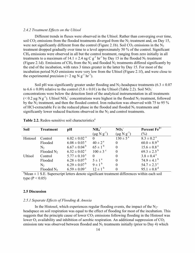
2.4.2 Treatment Effects on the Ultisol

Different trends in fluxes were observed in the Ultisol. Rather than converging over time, soil CO2 emissions from the flooded treatments diverged from the N2 treatment and, on Day 15, were not significantly different from the control (Figure 2.1b). Soil CO2 emissions in the N2 treatment dropped gradually over time to a level approximately 50 % of the control. Significant CH4 emissions were observed in all but the control treatment, ranging from zero initially in all treatments to a maximum of 14.1 ± 2.4 ng C g-1 hr-1

by Day 15 in the flooded N2 treatment (Figure 2.1d). Emissions of CH4 from the N2 and flooded N2 treatments differed significantly by the end of the incubation, with rates 3 times greater in the latter by Day 15. For most of the incubation period N2O emissions were very low from the Ultisol (Figure 2.1f), and were close to the experimental precision (< 2 ng N g-1 hr-1).

Soil pH was significantly greater under flooding and N2-headspace treatments (6.3 ± 0.07

to 6.6 ± 0.09) relative to the control (5.8 ± 0.01) in the Ultisol (Table 2.2). Soil NO3-

concentrations were below the detection limit of the analytical instrumentation in all treatments (< 0.2 µg N g-1). Ultisol NH4

+ concentrations were highest in the flooded N2 treatment, followed by the N2 treatment, and then the flooded control. Iron reduction was observed with 75 to 95 % of HCl-extractable Fe in the reduced phase in the flooded and flooded N2 treatments and significantly lower reduced fractions observed in the N2 and control treatments. Table 2.2. Redox-sensitive soil characteristicsa Soil Treatment pH NH4

+ (µg N g-1)

NO3-

(µg N g-1) Percent Fe2+ (%)

Histosol Control 6.02 ± 0.02 a 0 130 ± 5 a 8.3 ± 0.2 a Flooded 6.08 ± 0.03 a 40 ± 2 a 0 60.0 ± 8.9 b N2 6.67 ± 0.04 b 65 ± 1 b 0 15.6 ± 0.8 a Flooded N2 6.52 ± 0.02 c 100 ± 3 c 0 69.3 ± 2.5 b Ultisol Control 5.77 ± 0.10 a 0 0 3.8 ± 0.4 a Flooded 6.28 ± 0.07 b 5 ± 1 a 0 74.9 ± 4.1 b N2 6.29 ± 0.07 b 9 ± 1 b 0 54.7 ± 2.3 c Flooded N2 6.59 ± 0.09 c 12 ± 1 b 0 95.1 ± 0.8 d

aMean ± 1 S.E. Superscript letters denote significant treatment differences within each soil type (P < 0.05) 2.5 Discussion 2.5.1 Separate Effects of Flooding & Anoxia

In the Histosol, which experiences regular flooding events, the impact of the N2-headspace on soil respiration was equal to the effect of flooding for most of the incubation. This suggests that the principle cause of lower CO2 emissions following flooding in the Histosol was lower O2 availability and inhibition of aerobic respiration. An additional suppression of CO2 emission rate was observed between flooded and N2 treatments initially (prior to Day 4) which

15

may be due to the dissolution of CO2 into added water, rather than an effect on CO2 production. In the tropical forest Ultisol, that rarely experiences flooding under natural conditions, the unflooded anaerobic treatment (i.e. N2 treatment) decreased CO2 emissions by ~50 % over the incubation, whereas flooding resulted in only a short-term decline followed by an increase in CO2 emissions that equaled the control treatment by the end of the incubation. Soil respiration increased in both flooded treatments between Day 8 and Day 15, while under an N2-headspace alone soil respiration continued to decline. These results are evidence that flooding and anoxia can have distinct effects on soil respiration.

There are several potential mechanisms that could have contributed to the patterns

observed in the Ultisol. Flooding may have enhanced the availability of non-O2 TEAs leading to more anaerobic respiration and CO2 production. Both greater methanogensis and greater Fe reduction observed in the flooded N2 treatment could be the source of additional CO2. Increases in soil pH during reduction can lead to solubilization of C and has been shown to be an important mechanism in highly weathered soils (Thompson et al. 2006; Wagai and Mayer 2007), however pH changes from an initial analysis in the present study were modest (0.4 – 0.8; data not shown). Flooding may have facilitated the destabilization of organo-mineral complexes and increased labile C availability relative to the unflooded, but anaerobic soil. Past studies have found that flooding can lead to soil disaggregation, dissolution of soluble constituents, and concurrent increases in soil solution dissolved organic C (DOC) availability (Ponnamperuma 1972; Suarez et al. 1984; Kirk et al. 2003; De-Campos et al. 2009). The Ultisol is characterized by high Fe-oxide content and organo-mineral associations in these soil types can contribute substantially to C storage (Silver et al. 1999; Dubinsky et al. 2010). Density fractionation performed on surface (0-10 cm) samples of the same Ultisol found that 78-88 % of total soil C was in the mineral-associated (dense) fraction (Hall et al. unpublished data). In contrast, free-light and occluded-light C fractions dominate Histosols, which did not exhibit a similar stimulation of CO2 or CH4 emission. We therefore propose that the physical disaggregation or reductive dissolution of organo-mineral complexes could have led to a release of formerly protected C that was then exposed to mineralization processes under flooding. In this way, flooding may act to influence soil redox conditions, not only by changing the dominant TEA processes, in this case O2 availability, but also by influencing the availability of C as electron donors. Our results show that flooding maintained elevated CO2 emissions relative to an N2 headspace treatment alone and thus we demonstrate a separate effect of flooding on anaerobic soil respiration rates in the Ultisol.

We detected no CH4 emissions from the Histosol. These soils have shown

methanogenesis under flooded conditions in the field (Teh et al. 2011) and the lack of net CH4 production during the 30 day laboratory incubation was surprising. However, other peatland soil incubation studies have observed delays of > 30 days for the onset of methanogenesis after re-flooding of experimentally dried soil (Estop-Aragonés and Blodau 2012) or partly drained peatland soil (Jerman et al. 2009). Iron reduction may have contributed to a competitive inhibition of CH4 production (Teh et al. 2006), as at least 30 % of the acid-extractable Fe was still present as Fe3+ by the end of the experiment in these Fe-rich peatland soils. Flooding stimulated net CH4 emissions under anaerobic conditions in the Ultisol. If CH4 production was predominantly via acetate-cleavage rather than hydrogenotrophic CO2 reduction (Conrad 1999;

16

Chasar et al. 2000; Ye et al. 2012), then increased labile C availability from flooding could have been responsible for the patterns observed.

Separate effects of flooding and O2 depletion alone were observed for Histosol N2O

fluxes with sustained net N2O emissions in the N2 treatment and zero N2O emission under flooding. Disappearance of N2O emissions under flooding may have been caused by more rapid NO3

- depletion; inhibiting further denitrification to N2O. The continued net N2O emission in the absence of flooding may be attributable to faster diffusion in the gas-filled pore spaces of the field moisture treatment. This interpretation follows from the ‘hole-in-the-pipe’ conceptual model proposed to explain patterns in NO, N2O, and N2 soil gas emissions (Firestone and Davidson 1989). The model proposes that soils with gas-phase pore spaces are more ‘leaky’ to gaseous intermediates during dentrification than low porosity or flooded soils (Bollman and Conrad 1998; Davidson et al. 2000). Headspace O2 removal and flooding may both lead to a loss of NO3

- (Table 2) via denitrification, but differences in the rate of NO3- reduction and

differences in soil diffusivity specifically associated with flooding may explain the observed treatment differences in N2O emission rates. 2.5.2 Quantitative Importance of Aerobic Respiration

In both soils, headspace O2 removal (N2 treatment versus control) resulted in a large (~50 %) suppression of respiration rates. Suppression was observed immediately (< 1 day) in the Histosol in contrast to a gradual decline in the Ultisol. The large, and sudden, response of the Histosol to reduced O2 availability supports recent research that has proposed a critical role for O2 in peatland C degradation. Oxygen is important as a high energy-yield TEA for the final step of C mineralization by soil microbes, but earlier steps are also dependent on available O2 such as the activity of extracellular oxidative enzymes. The inhibition of oxidative enzymes due to anoxia has been proposed to function as an enzymatic latch on soil C pools, for flooded or low redox soils in particular (Freeman et al. 2001; Sinsabaugh 2010). Thus direct inhibition of aerobic respiration likely explains the immediate drop in respiration, but the continued, more gradual, decline could be a result of reduced oxidative enzyme activity.

In the Ultisol a reduction in soil respiration (N2 treatment versus control) was not

observed until Day 3 and increased in magnitude only gradually thereafter. There are several potential explanations for this pattern. First, it is possible that aerobic microsites environments persisted in the high clay soil, and O2 continued to be consumed over the early period of the incubation. However it is also possible that alternative TEAs, such as the abundant Fe in these soils, dominated respiration even in aerobic conditions (control treatment) where they were regenerated by available O2, and that the gradual decline in respiration under N2 occurred as the alternative TEAs were exhausted. This interpretation is consistent with the emerging view that C cycling in clay-rich Ultisols found in tropical forests is driven by the rotation of the Fe3+-Fe2+ redox wheel (Chacón et al. 2006; Dubinsky et al. 2010; Li et al. 2012; Hall and Silver 2013) and may explain observed decoupling of soil respiration from moisture and O2 availability in situ (Hall et al. 2013). 2.5.3 Effects of O2 Availability on Flooded-soil Greenhouse Gas Emissions

17

The experimental design also allowed us to test the effects of higher versus lower O2 availability on flooded-soil biogeochemistry (flooded versus flooded N2 treatment). The flooded Histosol with an oxic headspace had very similar heterotrophic respiration rates to the flooded N2 treatment, indicating aerobic respiration was not quantitatively important under flooding. Minimal aerobic respiration is consistent with studies of wetland sediments or peatland soils that have measured dissolved O2 across fine spatial gradients and show depletion within a few millimetres or centimetres of the oxic interface (Takai and Kamura 1966; Askaer et al. 2010). In contrast, an oxic headspace was found to significantly suppress flooded-soil CH4 emissions in the Ultisol. Methanotrophic bacteria can couple the oxidation of CH4 to the reduction of O2 (Hanson and Hanson 1996). Assuming the treatment difference was entirely due to oxidation, we estimate that up to 80-85 % of CH4 was consumed during upward diffusion in the microcosm by the end of the incubation. Such strong attenuation of CH4 emissions has been observed in other systems dominated by diffusive fluxes; oxic-anoxic interfaces at rice-plant rhizospheres can consume up > 90 % of the net CH4 flux (Holzapfel-Pschorn et al. 1986) and oxygenated water-columns have also been shown to ameliorate CH4 emissions by up to 90 % (King 1990).

The rates of nitrification and denitrification, driven by higher and lower O2 availability

respectively, complement the concept of pore-space diffusivity to explain the distinct N2O emissions observed between the flooded and flooded N2 treatments. In the flooded Histosol we observed a large, though temporary, pulse in N2O emissions. The absence of a similar pulse of N2O emission in the flooded N2 treatment suggests the availability of O2 or an oxic headspace can influence the timing and magnitude of the pulse. We include timing as well as magnitude because we cannot exclude the possibility that we missed a brief pulse in N2O emission that occurred before Day 1 in the flooded N2 treatment. Similar pulses have been repeatedly observed during soil wet-up experiments, during periods of high soil water-filled pore space, and during in situ precipitation or flooding events across a range of soil types (Keller and Reiners 1994; Hungate et al. 1997; Teh et al. 2011; Jørgensen and Elberling 2012). Such events are typically attributed to a stimulation of denitrification during soil reduction (Conrad 1996) however given the presence of O2 in the water used to flood the soil we cannot exclude a contribution from nitrification in the flooded treatment (Firestone and Davidson 1989). The greater dissolved O2 present in the flooded treatment initially may have led to greater N2O production by temporarily stimulating nitrification, by favoring incomplete denitrification to N2O, and/or by providing a larger or more persistent NO3

- supply for denitrification. Though we cannot isolate relative impacts on nitrification versus denitrification, our results indicate that large pulses of N2O emissions associated with soil wet-up or flooding are strongly dependent upon soil O2 availability. 2.6 Conclusions

Soil greenhouse gas emissions are strongly controlled by soil redox conditions. Flooding is generally assumed to precede redox changes; some soils, however, experience soil gas-phase anoxia without pore-space saturation. Here we asked how gas emissions differ under these distinct scenarios. We found that the size and magnitude of greenhouse gas emissions differ across the headspace and flooding treatments for two biogeochemically distinct soils. We found that in an Ultisol the effects of flooding on soil respiration could be divided into an effect of O2

18

removal and a separate effect, perhaps due to changes in the transport and/or availability of dissolve solutes following soil inundation. Emissions of N2O in both a Histosol and an Ultisol were likely sensitive to changes in pore-space diffusivity associated with flooding, in addition to the redox manipulations. Interestingly only the Ultisol, and not the Histosol, produced significant CH4 effluxes in the anaerobic incubation and these were significantly greater with flooding. We propose that the observation of elevated anoxic soil respiration and CH4 emission rates under flooding warrants further investigation to better identify the responsible biogeochemical mechanisms. 2.7 Acknowledgements

We thank Luke Lintott, Andrew McDowell, Carlos Torrens, Michelle Wong, and Wendy Yang for their assistance with practical aspects of sample collection, preparation, and analysis, and Steven Hall for assistance with statistical modeling of results. We also thank Daniel Richter and anonymous reviewers for useful comments on earlier versions of this manuscript. This research was supported by NSF grant EAR-08199072 to WLS, the NSF Luquillo Critical Zone Observatory (EAR-0722476) with additional support provided by the USGS Luquillo WEBB program, and grant DEB 0620910 from NSF to the Institute for Tropical Ecosystem Studies, University of Puerto Rico, and to the International Institute of Tropical Forestry USDA Forest Service, as part of the Luquillo Long-Term Ecological Research Program. Funding was also supplied by NSF grants ATM-0842385 and DEB-0543558 to WLS. 2.8 References Askaer, L., B. Elberling, R. N. Glud, M. Kuhl, F. R. Lauritsen, and H. P. Joensen (2010), Soil heterogeneity effects on O2 distribution and CH4 emissions from wetlands: in situ and mesocosm studies with planar O2 optodes and membrane inlet mass spectrometry, Soil Biol. Biochem., 42, 2254-2265. Beinroth, F. H. (1982), Some highly weathered soils of Puerto Rico, 1. Morphology, formation and classification, Geoderma, 27, 1-73. Bollman, A., and R. Conrad (1998), Influence of O2 availability on NO and N2O release by nitrification and denitrification in soils, Glob. Change Biol., 4, 387-396. Chacón, N., W. L. Silver, E. A. Dubinsky, D. F. Cusack, (2006), Iron reduction and soil phosphorous solubilization in humid tropical forest soils: the roles of labile carbon pools and an electron shuttle compound, Biogeochemistry, 78, 67-84. Chasar, L. S., J. P. Chanton, P. H. Glaser, D. I. Siegel, and J. S. Rivers (2000), Radiocarbon and stable isotopic evidence for transport and transformation of dissolved organic carbon, dissolved inorganic carbon, and CH4 in a northern Minnesota peatland, Glob. Biogeochem. Cycles, 14, 1095–1108.

19

Cleveland, C. C., W. R. Wieder, S. C. Reed, and A. R. Townsend (2010), Experimental drought in a tropical rain forest increases soil carbon dioxide losses to the atmosphere, Ecology, 91, 2313-2323. Conrad, R. (1996), Soil Microorganisms as controllers of atmospheric trace gases, Microbiol. Reviews, 60, 609-640. Conrad, R. (1999), Contribution of hydrogen to methane production and control of hydrogen concentrations in methanogenic soils and sediments, FEMS Microbiol. Ecol., 28, 193–202. Cusack, D. F., W. L. Silver, M. S. Torn, S. D. Burton, and M. K. Firestone (2011), Changes in microbial community characteristics and soil organic matter with nitrogen additions in two tropical forests, Ecology, 92, 621-632. Davidson, E. A., M. Keller, H. E. Erickson, L. V. Verchot, and E. Veldkamp (2000), Testing a conceptual model of soil emissions of nitrous and nitric oxides, Bioscience, 50, 667-680. DeAngelis, K. M., W. L. Silver, A. W. Thompson, and M. K. Firestone (2010), Microbial communities acclimate to recurring changes in soil redox potential status, Environ microbiol, 12, 3137-3149. De-Campos, A., A. Mamedov, and C. Huang (2009), Short-term reducing conditions decrease soil aggregation, Soil Sci. Soc. Am. J., 73, 550-559. Drexler, J. (2011), Peat formation processes through the millennia in tidal marshes of the Sacramento-San Joaquin Delta, California, USA, Estuaries and Coasts, 34, 900-911. Dubinsky, E. A., W. L. Silver, and M. K. Firestone (2010), Tropical forest soil microbial communities couple iron and carbon biogeochemistry, Ecology, 91, 2604-2612. Estop-Aragonés, C., and C. Blodau (2012), Effects of experimental drying intensity and duration on respiration and methane production recovery in fen peat incubations, Soil Biol. Biochem. 47, 1-9. Firestone, M. K., and E. A. Davidson (1989), Microbiological basis of NO and N2O production and consumption in soil, in Exchange of trace gases between terrestrial ecosystems and the atmosphere, edited by M. O. Andrea and D. S. Schimel, pp. 7-21, Wiley, New York. Forster, P., V. Ramaswamy, P Artaxo, et al (2007), Chapter 2: Changes in atmospheric constituents and in radiative forcing, in Climate Change 2007: the physical science basis. Contribution of Working Group I to the fourth assessment report of the intergovernmental panel on climate change, edited by S. Solomon, D. Qin, M. Manning, Z. Chen, M. Marquis, K. B. Averyt, M. Tignor, H. L. Miller, Cambridge University Press, Cambridge, United Kingdom and New York, NY, USA.

20

Freeman, C., M. A. Lock, and B. Reynolds (1993), Fluxes of CO2, CH4, and N2O from a Welsh peatland following simulation of water table draw-down: potential feedback to climate change, Biogeochemistry, 19, 51-60. Freeman, C., N. Ostle, and H. Kang (2001), An enzymatic ‘latch’ on a global carbon store, Nature, 409, 149. Grable, A. R., and E. G. Siemer (1968), Effects of bulk density, aggregate size, and soil water suction on oxygen diffusion, redox potentials, and elongation of corn roots, Soil Sci. Soc. Am. J., 32, 180-186. Hall, S. J., W. H. McDowell, and W. L. Silver (2013), When wet gets wetter: decoupling of moisture, redox biogeochemistry, and greenhouse gas fluxes in a humid tropical forest soil, Ecosystems, 16, 576-589. Hall, S. J., and W. L. Silver (2013), Iron oxidation stimulates organic matter decomposition in humid tropical forest soils, Glob. Change Biol., doi:10.1111/gcb.12229. Hanson, R.S., and T. E. Hanson (1996), Methanotrophic bacteria, Microbiol. Reviews, 60, 439-471. Holzapfel-Pschorn, A., R. Conrad, and W. Seiler (1986), Effects of vegetation on the emission of methane from submerged paddy soil, Plant and Soil, 92, 223-233. Hungate, B. A., C. P. Lund, H. L. Pearson, and F. S. Chapin III (1997), Elevated CO2 and nutrient addition alter soil N cycling and N trace gas fluxes with early season wet-up in a California annual grassland, Biogeochemistry, 37, 89-109. Jerman, V., M. Metje, I. Mandić-Mulec, and P. Frenzel (2009), Wetland restoration and methanogenesis: the activity of microbial populations and competition for substrates at different temperatures, Biogeosciences, 6, 1127-1138. Jørgensen, C. J., and B. Elberling (2012), Effects of flooding-induced N2O production, consumption and emission dynamics on the annual N2O emission budget in wetland soil, Soil Biol. Biochem., 53, 9-17. Keller, M., and W. A. Reiners (1994), Soil-atmosphere exchange of nitrous oxide, nitric oxide, and methane under secondary succession of pasture to forest in the Atlantic lowlands of Costa Rica, Glob. Biogeochem. Cycles, 8, 399-409. King, G. M. (1990), Regulation by light of methane emission in a wetland, Nature, 345, 513-515. Kirk, G. J. D., J. L. Solivas, and M. C. Alberto (2003), Effects of flooding and redox conditions on solute diffusion in soil, Eur. J. Soil Sci., 54, 617-624.

21

Li, Y., S. Yu, J. Strong, and H. Wang (2012), Are the biogeochemical cycles of carbon, nitrogen, sulfur, and phosophorus driven by the “FeIII-FeII redox wheel” in dynamic redox environments?, J. Soils and Sediments, 12, 683-693. Linn, D. M., and J. W. Doran (1982), Effect of water-filled pore space on carbon dioxide and nitrous oxide production in tilled and nontilled soils, Soil Sci. Soc. Am. J., 48, 1267-1272. Liptzin, D., W. L. Silver, and M. Detto (2010) Temporal dynamics in soil oxygen and greenhouse gases in two humid tropical forests, Ecosystems, 14, 171-182. Lovley, D. R., E. J. P. Phillips, and D. J. Lonergan (1991), Enzymatic versus nonenzymatic mechanisms for Fe3+ reduction in aquatic sediments, Environ Sci. and Technol., 25, 1062-1067. Magnusson, T. (1992), Studies of the soil atmosphere and related physical site characteristics in mineral forest soils, J. Soil Sci., 43, 767-790. Megonigal, J. P., M. E. Hines, and P. T. Visscher (2004), Anaerobic metabolism: Linkages to trace gases and aerobic processes, in Biogeochemistry Vol. 8 Treatise on Geochemistry, edited by W. H. Schlesinger, pp 317-424, Elsevier-Pergamon, Oxford, UK. Mitchell, J. K., and K. Soga, (1993), Fundamentals of soil behavior, pp 325-345, Wiley, New York. Nye, P. H. (1979), Diffusion of ions and uncharged solutes in soils and soil clays, Advances in Agronomy, 31, 225–272. Patrick Jr, W. H., and K. R. Reddy (1976), Nitrification-denitrification reactions in flooded soils and water bottoms: dependence on oxygen supply and ammonium diffusion, J. Environ. Qual., 5, 469–472. Peters, V., and R. Conrad (1996), Sequential reduction and initiation of CH4 production upon flooding of oxic upland soils, Soil Biol. Biochem., 28, 371-382. Pett-Ridge, J., W. Silver, and M. Firestone (2006), Redox fluctuations frame microbial community impacts on N-cycling rates in a humid tropical forest soil, Biogeochemistry, 81, 95-110. Ponnamperuma, F. N. (1972), The chemistry of submerged soils, Adv. in Agron., 24, 29-96. Raich, J. W., and C. S. Potter (1995), Global patterns of carbon dioxide emissions from soils, Glob. Biogeochem. Cycles, 9, 23-36. Regina, K., J. Silvola, and P. J. Martikainen (1999), Short-term effects of changing water table on N2O fluxes from peat monoliths from natural and drained boreal peatlands, Glob. Change Biol., 5, 183-189. Roden, E. E., and R. G. Wetzel (1996), Organic carbon oxidation and suppression of methane production by microbial Fe(III) oxide reduction in vegetated and unvegetated freshwater wetland sediments, Limnol. Oceanogr., 41, 1733-1748.

22

Schuur, E. A. G. (2001), The effects of water on decomposition dynamics in mesic to wet Hawaiian montane forests, Ecosystems, 4, 259-273. Silver, W.L., A. E. Lugo, and M. Keller (1999), Soil oxygen availability and biogeochemistry along rainfall and topographic gradients in upland wet tropical forest soils, Biogeochemistry, 44, 301-328. Silver, W. L., D. Liptzin, and M. Almaraz (2013), Soil redox dynamics and biogeochemistry along a tropical elevation gradient, Ecol. Bull., in press. Sinsabaugh, R. L. (2010), Phenol oxidase, peroxidase and organic matter dynamics of soil, Soil Biol. Biochem., 42, 391-404. Stookey, L. L. (1970), Ferrozine – a new spectrophotometric reagent for iron, Anal. Chem., 42,779-781. Suarez, D. L., J. D. Rhoades, R. Lavado, and C. M. Grieve (1984), Effect of pH on saturated hydraulic conductivity and soil dispersion, Soil Sci. Soc. Am. J., 48, 50-55. Takai, Y., and T. Kamura (1966), The mechanism of reduction in waterlogged paddy soil, Folia Microbiol., 11, 304-313. Teh, Y. A., W. L. Silver, and M. E. Conrad (2005), Oxygen effects on methane production and oxidation in humic tropical forest soils, Glob. Change Biol., 11, 1283-1297. Teh, Y. A., and W. L. Silver (2006), Effects of soil structure destruction on methane production and carbon partitioning between methanogenic pathways in tropical rain forest soils, J. Geophys. Res., 111, G01003. Teh, Y. A., W. L. Silver, O. Sonnentag, M. Detto, M. Kelly, and D. D. Baldocchi (2011), Large greenhouse gas emissions from a temperate peatland pasture, Ecosystems, 14, 311-325. Thompson, A., O. A. Chadwick, S. Boman, and J. Chorover (2006), Colloid mobilization during soil iron redox oscillations, Environ. Sci. Technol., 40, 5743-5749. Viollier, E., Inglett, P. W., Hunter, K., Roychoudhury, P., and P. Van Cappellen (2000), The ferrozine method revisited: Fe(II)/Fe(III) determination in natural waters, Applied Geochemistry, 15, 785-790. Wagai, R., and L. M. Mayer (2007), Sorptive stabilization of organic matter in soils by hydrous iron oxides, Geochim Cosmochim Ac , 72, 25-35. Yang, W. H., Y. A. Teh, and W. L. Silver (2011), A test of a field-based 15N-nitrous oxide pool dilution technique to measure gross N2O production in soil, Glob. Change Biol., 17, 3577-3588.

23

Yang, W. H., D. Herman, D. Liptzin, and W. L. Silver (2012), A new approach for removing iron interference from soil nitrate analysis, Soil Biol. Biochem., 46, 123-128. Ye, R., Q. Jin, B. Bohannan, J. K. Keller, S. A. McAllister, and S. D. Bridgham (2012), pH controls over anaerobic carbon mineralization, the efficiency of methane production, and methanogenic pathways in peatlands across an ombrotrophic-minerotrophic gradient, Soil Biol. Biochem., 54, 36-47.

24

Chapter 3: Non-linear response of carbon dioxide and methane emissions to oxygen availability in a drained Histosol2

Scientific theories serve to facilitate the survey of our observations and experimental findings. Every scientist knows how difficult it is to remember a moderately extended group of facts, before at least some primitive theoretical picture about them has been shaped. It is therefore

small wonder, and by no means to be blamed on the authors of original papers or of text-books, that after a reasonably coherent theory has been formed, they do not describe the bare facts they have found or wish to convey to the reader, but clothe them in a terminology of that theory or

theories. This procedure, while very useful for remembering the facts in a well-ordered pattern, tends to obliterate the distinction between the actual observations and the theory arisen from them. And since the former always are of some sensual quality, theories are easily thought to

account for sensual qualities; which, of course, they never do. - Erwin Schrödinger Mind and Matter [1956]

3.1 Abstract

Organic-rich wetland soils in the Histosol soil order represent the largest soil carbon (C) pool globally. Carbon accumulation in these ecosystems is largely due to oxygen (O2) limitation of decomposition. Increased O2 availability from wetland drainage and climate change may stimulate C decomposition overall and affect the balance of carbon dioxide (CO2) and methane (CH4) greenhouse gas release. Characterizing relationships, including non-linearity, between soil O2 and C gas emissions is therefore critical to predict the partitioning and rate of C release from Histosols under greater O2 availability. We varied gas-phase O2 concentration from 0.03 to 20 % in incubations of a sapric Histosol and measured resulting CO2 and CH4 emissions. Efflux of CO2 increased and CH4 emissions decreased at higher O2 concentrations, and rates were best described by log-linear model fits. The non-linear response of CO2 and CH4 emissions to O2 concentration indicates that moist, C rich Histosols may be highly sensitive to increases in O2 availability, even below concentration thresholds typically classified as anoxic. 2 This chapter is reprinted, with permission, from the original journal article: McNicol G, Silver WL (2015) Non-linear response of carbon dioxide and methane emissions to oxygen availability in a drained Histosol. Biogeochemistry 123(1-2): 299-306

25

3.2 Introduction

Carbon-rich Histosols found in peatlands and other wetland ecosystems contain as much as one-third of Earth’s soil carbon (C) pool (Limpens et al. 2008). Globally many Histosols have been drained for agriculture leading to large C losses and altered patterns of greenhouse gas emissions. Increased soil organic C oxidation and associated carbon dioxide (CO2) emissions following drainage or natural drying of the soil have been documented in temperate (Schothorst 1977; Moore and Knowles 1989; Deverel and Rojstaczer 1996; Kasimir-Klemedtsson et al. 1997; Nieveen et al. 2005; Teh et al. 2011; Hatala et al. 2012), high-latitude (Jungkunst and Fiedler 2007; Silvola et al. 2009; Sulman et al. 2009), and tropical (Moore et al. 2013) peatland Histosols. Soil drying and water table drawdown in some regions under predicted climatic changes may have similar effects on Histosol C stocks and fluxes (Laiho 2006; Limpens et al. 2008).

The availability of oxygen (O2) is a critical control on rates of Histosol C loss as it

activates key oxidative enzymes necessary for extracellular breakdown of inhibitory phenolic compounds and permits energetically favorable aerobic respiration (Clymo 1984; Freeman et al. 2001; Freeman et al. 2004; Laiho 2006; Teh et al. 2011; Philben et al. 2014). Drainage of wetlands exposes Histosols to elevated O2

(Laiho 2006), which can increase short-term rates of CO2 emissions by two-fold or more compared to anaerobic conditions (Moore and Dalva 1993; Silvola et al. 1996; Blodau and Moore 2003; Chimner and Cooper 2003; Glatzel et al. 2004; McNicol and Silver 2014). Drainage also dramatically decreases Histosol emissions of methane (CH4), a greenhouse gas 34 times more potent than CO2 over a 100-year timescale (Myhre et al. 2013), by facilitating aerobic microbial methanotrophy in drained soil layers (Sundh et al. 1994; Hanson and Hanson 1996; Whalen 2005). Though vegetation composition, nutrient availability, substrate quality, and temperature also regulate rates of soil C emissions across distinct wetland Histosols (Bridgham et al. 2006), O2 is a direct mechanistic control on both CO2 and CH4 emissions.

Over short timescales the release of CO2 and CH4 from Histosols is strongly influenced

by rates of aerobic microbial respiration and CH4 consumption (methanotrophy), which are by definition dependent on available O2. However, to our knowledge, no studies have explicitly characterized the kinetic response of these aerobic processes at aggregate-to-pedon scale to the wide range of gas-phase O2 concentration possible in situ (0-21 %). Oxygen is likely to occur at very low concentrations in soil air under conditions of high biological O2 demand and a tortuous gas-phase diffusion environment (Grable and Siemer 1968; Silver et al. 1999; Teh et al. 2005; Hall et al. 2012), such as soils at depth in peatlands. With the exception of microaerophilic methanotrophs (Hanson and Hanson 1996), we have surprisingly little understanding of how processes important to Histosol C gas exchange are affected by low soil O2 concentrations (< 1 %) that are functionally equated with anoxic conditions in geochemical redox classifications (Berner 1981; Scott and Morgan 1990; Chapelle et al. 1995). Most soil microcosm studies that manipulate O2 concentration have imposed coarse (Teh et al. 2005) or narrow (Greenwood 1961) ranges, which are aptly suited for mechanistic investigations, but cannot characterize a kinetic response relevant to the wide range of potential in situ O2 concentrations. Extant studies that contrast oxic and anoxic conditions function as useful end-members, but are insufficient to

26

investigate non-linearity. Non-linear relationships, common in biophysical systems, and are important to identify and characterize to accurately predict responses to environmental variance (Ruel and Ayres 1999). In the case of Histosols, non-linear effects of O2 must be represented to accurately model C biogeochemical processes. Indeed recent modeling work shows that improved representation of soil O2 availability better predicts C fluxes from peatland Histosols (Fan et al. 2014).

There are both intrinsic and extrinsic factors that could lead to non-linearity between soil

O2 availability and emission of CO2 and CH4. Standard Michaelis-Menten enzyme kinetics that govern the intrinsic reaction rates of microbially mediated soil processes would predict a non-linear response of aerobic respiration or CH4 consumption to O2 concentration. Extrinsic factors, such as substrate availability (labile C or CH4) or slow diffusive gas transport, could also lead to asymptotic relationships between O2 consuming processes and O2 concentration (Davidson and Janssens 2006). In this study, we test the hypothesis that the aerobic processes underlying CO2 and CH4 emissions from peatland soils are highly sensitive to O2, resulting in asymptotic, non-linear relationships between C gas fluxes and O2 concentrations. To test this hypothesis we measured the short-term responses of CO2 and CH4 emissions in incubations of a drained peatland Histosol to a wide range of gas-phase O2 concentrations. 3.3 Method

We collected approximately 6 kg of soil from the vadose zone-water table interface in a drained peatland pasture located on Sherman Island, in the Sacramento San-Joaquin Delta, CA. Similar to other Delta regions globally, the Sacramento Delta has experienced extensive land reclamation over the last 150 years (Deverel and Rojstaczer 1996). The contemporary soil profile consists of a 25 to 92 cm oxidized layer overlying a thick sapric peat horizon (Table 3.1) (Drexler et al. 2009). We used peat soil from 80-100 cm depth that straddles the water table and therefore has only undergone slight oxidation and is classified as a sapric Histosol (mucky peat). Soils at this depth were wet, but not saturated at the time of collection (Table 3.1); moisture increases seasonally to saturation in summer-time due to managed water table increases. Soil CN concentration and bulk density by depth are reported in Table 3.1 (unpublished data). Steep, persistent O2 concentration gradients with depth have been observed at the site (Figure 3.1). Data are averages of hourly gas-phase O2 measurements collected in March 2012 (n = 744) using calibrated galvanic cell sensors (Apogee Instruments, Logan, Utah) installed at 10, 20, and 30 cm in watertight PVC cylinders with a Gore-Tex seal at one end that permitted soil-chamber gas exchange (Liptzin et al. 2010). The soil exhibits a consistent structure composed of fine (~mm) spherical aggregates with low bulk density (Table 3.1), thus only gentle mixing by hand was required to homogenize slight moisture differences within the sampled soil. Any stones and green plant material introduced during soil collection were removed in the laboratory before approximately 200 g samples were transferred to either 1 L (946 cm3) (higher O2 treatments) or 4 L (3,786 cm3) sized Mason jars (lower O2 treatments). Larger jars were used for low O2 treatments to minimize the effect of O2 consumption and sample removal on headspace O2 concentrations during the incubation. The jar headspace was made anaerobic using a 2 hr pre-incubation in a glovebox and purging the headspace with Ultra-High Purity (UHP) N2 (Praxair, Richmond, CA) at 10 PSI. Flow rates and timing required for removing O2 below detectable

27

limits were determined a priori using a galvanic cell sensor (Apogee Instruments, Logan, Utah). Jars were then fitted with gas-tight lids and incubated in the dark (i.e. in boxes) to prevent phototrophic CO2 consumption.

Table 3.1. Soil classification and characteristics at 80 cm depth in profile (mean ± SE).

Soil Classification

Site Location

C/N (%)

Moisture (%)

Bulk Density (g cm-3)

Porosity*

Typic Haplosaprists

Sherman Island, CA

23.7 ± 3.0/ 1.1 ± 0.1 62 ± 1 0.25 0.84

Figure 3.1. Average O2 concentrations (mean ± 1 SD) with depth (10, 20, 30 cm) in drained peatland pasture Sherman Island, CA, collected hourly (n = 744) in March 2012

Seven O2 treatment levels (0.03, 0.1, 0.3, 1, 3, 10, 20 %; n = 4) were achieved by

quantitative additions of either Ultra-Zero Air (19.5-23.5 % O2, balance N2), or UHP O2 (99.993 % O2; Praxair, Richmond, CA). Treatment O2 concentrations below 0.03 % were not attempted because the precision with which the residual O2 concentration in jars after N2 flushing was known at the same order-of-magnitude as the lowest O2 treatment (± 0.01 % O2). Headspaces were mixed 10 times with a 10 ml syringe after O2 additions and 20 ml headspace subsamples were taken immediately after mixing, and after 2, 4, and 6 h of incubation. Incubations were conducted at room temperature (21 °C) and significant pressure changes were avoided by replacing headspace after sample removal with either UHP N2 (low O2 treatments), 10 % O2 in N2 (10 % treatment), or Ultra-Zero Air (20 % treatment). Gas (CO2 and CH4) concentrations were determined on a Shimadzu GC-14A gas chromatograph (Shimadzu Scientific Inc., Columbia, Maryland, USA) equipped with TCD and FID detectors and calibrated with standard gas containing 997 ppm(v) CO2 and 9.91 ppm(v) CH4.

0 7 14 21

-35

-25

-15

-55

O2 Concentration (%)

Dep

th (c

m)

Water-table

28

Fluxes were computed from the linear term of a second-order polynomial fit (CO2 flux)

or linear fit (CH4) and accepted if fit R2 ≥ 0.99 (12.5 % fluxes rejected). Flux data were plotted against O2 concentration with both linear and log-linear regressions, and fits were compared using the coefficient of determination (R2) and the distribution of residuals as performance metrics. Direct comparison of the R2 is a fair metric for significant relationships (P < 0.001) in this case because only one parameter is being estimated in both linear and log-linear fits, for [O2] and log10[O2], respectively. Quasi-Michaelis-Menten (qMM) parameters (maximum reaction velocity (qVmax) and half saturation constants (qkMO2)) were estimated by normalizing fluxes to the mean flux observed at the lowest O2 concentration treatment (0.03 %) that forced model fits through the origin. We qualify the parameters as qMM as they are not strict measures of single-enzyme reaction rates. Simultaneous effects of O2 on both aerobic and anaerobic processes (e.g. CH4 oxidation and production) and other limiting factors, such as rates of diffusive gas transport across the soil air-water boundary or C substrate availability, mean the qMM parameters should be interpreted without mechanistic specificity. All data analysis was performed in open-source statistical software package, R (v. 2.15.2, Vienna, Austria). 3.4 Results

Mean soil CO2 emissions significantly increased (P < 0.001) with increasing O2 concentration (Figure 3.2a,b; Table 2) from 180 ± 5 µg C g-1 d-1 at 0.03 % O2 to 227 ± 16 µg C g-

1 d-1 at 20 % O2. A log-linear fit outperformed a linear model fit to all data by both metrics: log-linear R2 was 0.49 in contrast to 0.38 for the linear model (Table 3.2), and the residuals more closely approximated a normal distribution (Figure 3.3a,b) with less skewing at lower fitted values. Crucially, the modeled y-intercept (background anaerobic respiration rate) was much lower with the log-linear fit (126 µg C g-1 d-1) than the linear fit (186 µg C g-1 d-1), thus the total modeled effect of oxic conditions (~20 % O2) on respiration was thus much larger with the log-linear fit (75 % increase) compared to the linear fit (24 % increase). After normalizing data by lowest O2 treatment we extracted a qVmax for aerobic respiration of 47.3 µg C g-1 d-1 and qkMO2 of 2.2 % O2.

Table 3.2. Coefficients and fits of linear, log-linear (Log), and Michaelis-Menten (MM) models

Gas Fit p-value R2 Y-intercept (µg C g-1 d-1)

O2 Effect (%)

qVmax (µg C g-1 d-1)

qkMO2 (%)

CO2 Linear < 0.001 0.38 186 +24 - - Log < 0.001 0.49 126 +75 - - MM - - - - 47.3 2.2

CH4 Linear < 0.001 0.40 0.21 -257 - - Log < 0.001 0.70 0.42 -383 - - MM - - - - -0.18 0.2

29

Figure 3.2. CO2 flux (a, b; µg C g-1 d-1) and CH4 flux (c, d; ng C g-1 d-1) versus O2 concentration ([O2] (ppm(v))) on untransformed x-axis (a, c) and log10 transformed (b, d) x-axis. Dashed line, coefficients, R2 and p-values are for log-linear model fit

Mean soil CH4 emissions decreased (P < 0.001) with increasing O2 concentration (Figure

3.2c, d) from 303 ± 32 ng C g-1 d-1 at 0.03 % to 77 ± 11 ng C g-1 d-1 at 20 % O2. A log-linear model greatly outperformed a linear model fit by both metrics: log-linear R2 was 0.70 compared to 0.40 for the linear fit (Table 3.2), and the residuals vs. fitted value distribution improved with the log-linear fit (Figure 3.3c, d). The modeled y-intercept (background CH4 production rate) was twice as large (0.42 µg C g-1 d-1) for the log-linear fit, than for the linear fit (0.21 µg C g-1 d-

1), and the modeled effect of 20 % O2 was thus proportionally larger (-383 % for log-linear vs. -257 % for linear). After normalization we extracted a qVmax for aerobic methanotrophy of -0.18 µg C g-1 d-1 and a qkMO2 of 0.2 %.

0 50000 100000 150000 200000

160

180

200

220

240

260

Headspace [O2] (ppm)

CO2

Flux

(µg

C g-1

d−1)

a

R2 = 0.49p < 0.0001y = 126 + 18(log10[x])

2.5 3.0 3.5 4.0 4.5 5.0

160

180

200

220

240

260

Headspace log10[O2] (ppm)

CO2

Flux

(µg

C g-1

d−1)

b

0 50000 100000 150000 200000

0100

200

300

400

Headspace [O2] (ppm)

CH4

Flux

(ng

C g-1

d−1)

cR2 = 0.70p < 0.0001y = 422 - 63(log10[x])

2.5 3.0 3.5 4.0 4.5 5.0

0100

200

300

400

Headspace log10[O2] (ppm)

CH4

Flux

(ng

C g-1

d−1)

d

30

Figure 3.3. Residuals vs. fitted values for CO2 flux (a, b; µg C g-1 d-1) and CH4 flux (c, d; ng C g-

1 d-1) from linear (a, c) and log-linear (b, d) model fits. 3.5 Discussion

We found that heterotrophic respiration rates increased with greater available gas-phase

O2 as would be anticipated given the favorable conditions for aerobic decomposition: namely moist, C--rich soil, not yet at steady-state with the oxidizing atmosphere (Clymo 1984; Laiho 2006; Philben et al. 2014). Importantly, we found that a log-linear model better described the relationship than a linear model and the approximated qkMO2 indicated a high sensitivity of aerobic respiration rates to available O2 with 50 % of stimulated respiration occurring below 2.2 % O2. This stands in contrast to geochemical characterizations of soil redox that often refer to soils as functionally anoxic below a 1 % gas-phase O2 concentration (Berner 1981; Scott and Morgan 1990; Chapelle et al. 1995). Other soils, however, may display varying degrees of O2 sensitivity where other extrinsic factors become rate limiting, such as soluble C substrate supply,

a b

c d

31

or where constraints imposed by the gas-phase diffusion environment restrict O2 transport (Davidson and Janssens 2006). For example, we have previously observed a similarly large effect of headspace O2 removal on heterotrophic respiration rates in a peatland Histosol, whereas no immediate effect was observed in a tropical Ultisol collected from the Luquillo Experimental Forest, Puerto Rico (McNicol and Silver 2014). Notably, the predicted y-intercept, which reflects the estimated rate of background anaerobic respiration, was much lower in the log-linear model (126 µg C g-1 d-1) than the linear model (186 µg C g-1 d-1). This highlights the potential for errors arising from incorrect kinetic characterization of the impact of low O2 concentrations – such as those found at depth in drained peatlands – on process models that incorporate microbial function. Regardless of fit, absolute rates of predicted anaerobic respiration are higher than would be expected in C accumulating Histosols. We suggest this is due to high alternative electron acceptor availability, the sapric quality of the peat, and the low water-table position. In particular, the drained deltaic Histosol used in this study has a large acid-extractable Fe pool (>1 mg Fe g-1; McNicol and Silver, unpublished data) that is ~40% Fe(III) at the water-table interface (McNicol and Silver, 2014). The CO2 emission data suggest that substantial stimulation of CO2 production may be possible in moist, C-rich Histosols at low O2 concentrations.

Histosol CH4 emissions were greatly attenuated at higher O2 concentrations and this was

likely due to a shift toward more aerobic, and fewer anaerobic, soil microsites favoring greater CH4 consumption, and less CH4 production overall (Silver et al. 1999; von Fischer and Hedin 2007). Improvements by fitting a log-linear model were particularly apparent for CH4 emissions and the approximated qkMO2 of 0.2 % indicates a very strong O2 sensitivity. Although we did not experimentally isolate CH4 consumption, this strong sensitivity to O2 is consistent with a micro-aerophilic community of methanotrophs (Hanson and Hanson 1996) and observed maxima in gross CH4 consumption rates immediately above the water table in peatland Histosols where O2 availability is well below atmospheric concentrations (Sundh et al. 1994; Limpens et al. 2008). Further work is needed to evaluate the short-term O2 sensitivity of gross CH4 production and oxidation separately, but these data demonstrate that even very low (< 1%) gas-phase concentrations of O2 are sufficient to strongly attenuate CH4 fluxes in wetland soils. 3.6 Conclusions

Soil O2 is increasingly being measured in situ (Silver et al. 1999, 2013; Teh et al. 2005; Burgin and Groffman 2012; Hall et al. 2012; Philben et al. 2014). Though O2 is only one component of the soil redox environment, it is a highly favored oxidant with direct effects on microbial respiration and methanotrophy, and thus may be a useful measurement for linking redox biogeochemistry, microbial ecology, and soil-atmosphere exchange of greenhouse gases (Faulkner et al. 1989; Conrad 1996). In particular the large C pool contained globally in peatland Histosols is maintained by the low availability of O2 (Freeman et al. 2001; Freeman et al. 2004). Recent modeling efforts show it is necessary to consider the response of aerobic and anaerobic C cycling to the wide range of possible O2 concentrations in drained soil layers of peatland Histosols (Fan et al. 2014), yet surprisingly few data sets address biogeochemical sensitivity to O2. We varied O2 concentration across several orders of magnitude in laboratory incubations of a drained peatland Histosol to investigate the sensitivity of C gas emissions, and in particular the occurrence and importance of non-linearity. We found a log-linear fit best explained the response

32

of CO2 and CH4 emissions to O2 concentration. The results indicate non-linear O2 effects may be important to consider in soil C biogeochemical models because they predict different background (anaerobic) rates of C emission when compared to linear models, and can capture asymptotic effects of increasing O2 availability. In summary, the study used a novel O2 manipulation to identify non-linear relationships between O2 and Histosol C emissions, and demonstrated the sensitivity of emissions to low O2 conditions that are often functionally equated with anoxia. 3.7 Acknowledgements

This project was supported by the California Delta Stewardship Council via the Delta Science Program. G. M. was supported by a Lawrence Scholarship from Lawrence Livermore National Laboratory. Additional support was provided by UC-AES. We also thank the anonymous reviewers for comments that improved the manuscript. 3.8 References Berner RA (1981) A new geochemical classification of sedimentary environments. Journal of Sedimentary Research 51(2): 359-365 Blodau C, Moore TR (2003) Micro-scale CO2 and CH4 dynamics in a peat soil during a water fluctuation and sulfate pulse. Soil Biology and Biochemistry 35(4): 535-547 Bridgham SD, Megonigal JP, Keller JK, Bliss NB, Trettin C (2006) The carbon balance of North American wetlands. Wetlands 26(4): 889-916 Burgin AJ, Groffman PM (2012) Soil O2 controls denitrification rates and N2O yield in a riparian wetland. Journal of Geophysical Research: Biogeosciences 117(G1): G01010 Chapelle FH, McMahon PB, Dubrovsky NM, Fujii RF, Oaksford ET, Vroblesky DA (1995) Deducing the distribution of terminal electron-accepting processes in hydrologically diverse groundwater systems. Water Resources Research 31(2): 359-371 Chimner RA, Cooper DJ (2003) Influence of water table levels on CO2 emissions in a Colorado subalpine fen: An in situ microcosm study. Soil Biology and Biochemistry 35(3): 345-351 Conrad R (1996) Soil microorganisms as controllers of atmospheric trace gases (H2, CO, CH4, OCS, N2O, and NO). Microbiological Reviews 60(4): 609-640 Clymo RS (1984) The limits to peat bog growth. Philosophical Transactions of the Royal Society of London. Biological Sciences 303(1117): 605-654 Davidson EA, Janssens IA (2006) Temperature sensitivity of soil carbon decomposition and feedbacks to climate change. Nature 440(7081): 165-173

33

Deverel SJ, Rojstaczer S (1996) Subsidence of agricultural lands in the Sacramento-San Joaquin Delta, California: Role of aqueous and gaseous carbon fluxes. Water research 32(8): 2359-2367 Drexler JZ, de Fontaine CS, Deverel SJ (2009) The legacy of wetland drainage on the remaining peat in the Sacramento-San Joaquin Delta, California, USA. Wetlands 29(1): 372-386 Fan Z, Neff JC, Waldrop MP, Ballantyne AP, Turetsky MR (2014) Transport of oxygen in soil pore-water systems: Implications for modeling emissions of carbon dioxide and methane from peatlands. Biogeochemistry 121(3): 455-470 Faulkner SP, Patrick WH, Gambrell RP (1989) Field techniques for measuring wetland soil parameters. Soil Sci. Soc. Am. J. 53(3): 883-890 Freeman C, Ostle N, Kang H (2001) An enzymic 'latch' on a global carbon store. Nature 409(6817): 149-149 Freeman C, Ostle NJ, Fenner N, Kang H (2004) A regulatory role for phenol oxidase during decomposition in peatlands. Soil Biology and Biochemistry 36(10): 1663-1667 Glatzel S, Basiliko N, Moore T (2004) Carbon dioxide and methane production potentials of peats from natural, harvested and restored sites, eastern Québec, Canada. Wetlands 24(2): 261-267 Grable AR, Siemer EG (1968) Effects of bulk density, aggregate size, and soil water suction on oxygen diffusion, redox potentials, and elongation of corn roots. Soil Sci. Soc. Am. J. 32(2): 180-186 Greenwood DJ (1961) The effect of oxygen concentration on the decomposition of organic materials in soil. Plant and Soil 14(4): 360-376 Hall SJ, McDowell WH, Silver WL (2012) When wet gets wetter: Decoupling of moisture, redox biogeochemistry, and greenhouse gas fluxes in a humid tropical forest soil. Ecosystems 16(4): 576-589 Hanson RS, Hanson TE (1996) Methanotrophic bacteria. Microbio Mol Biol R 60(2): 439-463 Hatala JA, Detto M, Sonnentag O, Deverel SJ, Verfaillie J, Baldocchi DD (2012) Greenhouse gas (CO2, CH4, H2O) fluxes from drained and flooded agricultural peatlands in the Sacramento-San Joaquin Delta. Agriculture, Ecosystems and Environment 150: 1-18 Jungkunst HF, Fiedler S (2007) Latitudinal differentiated water table control of carbon dioxide, methane and nitrous oxide fluxes from hydromorphic soils: feedbacks to climate change. Global change biology 13(12): 2668-2683

34

Kasimir-Klemedtsson Å, Klemedtsson L, Berglund K, Martikainen P, Silvola J, Oenema O (1997) Greenhouse gas emissions from farmed organic soils: a review. Soil Use and Management 13: 245-250 Laiho R (2006) Decomposition in peatlands: Reconciling seemingly contrasting results on the impacts of lowered water levels. Soil Biology and Biochemistry 38(8): 2011-2024 Limpens J, Berendse F, Blodau C, Canadell JG, Freeman C, Holden J, Roulet N, Rydin H, Schaepman-Strub G (2008) Peatlands and the carbon cycle: from local processes to global implications – a synthesis. Biogeosciences 5(5): 1475-1491 Liptzin D, Silver WL, Detto M (2010) Temporal dynamics in soil oxygen and greenhouse gases in two humid tropical forests. Ecosystems 14(2): 171-182 McNicol G, Silver WL (2014) Separate effects of flooding and anaerobiosis on soil greenhouse gas emissions and redox sensitive biogeochemistry. Journal of Geophysical Research: Biogeosciences 119(4): 2013JG002433 Moore TR, Dalva M (1993) The influence of temperature and water table position on carbon dioxide and methane emissions from laboratory columns of peatland soils. Journal of Soil Science 44(4): 651-664 Moore S, Evans CD, Page SE, Garnett MH, Jones TG, Freeman C, Hooijer A, Wiltshire AJ, Limin SH, Gauci V (2013) Deep instability of deforested tropical peatlands revealed by fluvial organic carbon fluxes. Nature 493(7434): 660-663 Moore TR, Knowles R (1989) The influence of water table levels on methane and carbon dioxide emissions from peatland soils. Canadian Journal of Soil Science 69(1): 33-38 Myhre G, Shindell D, Bréon F-M, Collins W, Fuglestvedt J, Huang J, Koch D, Lamarque J-F, Lee D, Mendoza B, Nakajima T, Robock A, Stephens G, Takemura T, and Zhang H, (2013) Anthropogenic and Natural Radiative Forcing. In: Climate Change 2013: The Physical Science Basis. Contribution of Working Group I to the Fifth Assessment Report of the Intergovernmental Panel on Climate Change [Stocker TF, Qin D, Plattner G-K, Tignor M, Allen SK, Boschung J, Nauels A, Xia Y, Bex V, and Midgley PM, (eds.)]. Cambridge University Press, Cambridge, United Kingdom and New York, NY, USA. Nieveen JP, Campbell DI, Schipper LA, Blair IJ (2005) Carbon exchange of grazed pasture on a drained peat soil. Global change biology 11(4): 607-618 Oleszczuk R, Truba M (2013) The analysis of some physical properties of drained peat-moorish soil layers. Annals of Warsaw University of Life Sciences – SGGW. Land Reclamation 45(1): 41-48

35

Philben M, Kaiser K, Benner R (2014) Does oxygen exposure time control the extent of organic matter decomposition in peatlands? Journal of Geophysical Research: Biogeosciences 119(5): 2013JG002573 Ruel JJ, Ayres MP (1999) Jensen’s inequality predicts effects of environmental variation. Trends in Ecology and Evolution 14(9): 361-366 Schothorst CJ (1977) Subsidence of low moor peat soils in the western Netherlands. Geoderma 17(4): 265-291 Scott Michael J, Morgan James J (1990) Energetics and conservative properties of redox systems. In: Chemical Modeling of Aqueous Systems II. ACS Symposium Series, vol 416. American Chemical Society. pp 368-378 Silver WL, Lugo AE, Keller M (1999) Soil oxygen availability and biogeochemistry along rainfall and topographic gradients in upland wet tropical forest soils. Biogeochemistry 44(3): 301-328 Silver W, Liptzin D, Almaraz M (2013) Soil redox dynamics and biogeochemistry along a tropical elevational gradient. Ecol. Bull 4: 195-209 Silvola J, Alm J, Ahlholm U, Nykanen H, Martikainen PJ (1996) CO2 fluxes from peat in boreal mires under varying temperature and moisture conditions. Journal of Ecology 84(2): 219-228 Sundh I, Nilsson M, Granberg G, Svensson BH (1994) Depth distribution of microbial production and oxidation of methane in northern boreal peatlands. Microbial ecology 27(3): 253-265 Sulman BN, Desai AR, Cook BD, Saliendra N, Mackay DS (2009) Contrasting carbon dioxide fluxes between a drying shrub wetland in Northern Wisconsin, USA, and nearby forests. Biogeosciences 6(6): 1115-1126 Teh YA, Silver WL, Conrad ME (2005) Oxygen effects on methane production and oxidation in humid tropical forest soils. Global Change Biology 11(8): 1283-1297 Teh YA, Silver WL, Sonnentag O, Detto M, Kelly M, Baldocchi DD (2011) Large greenhouse gas emissions from a temperate peatland pasture. Ecosystems 14(2): 311-325 von Fischer JC, Hedin LO (2007) Controls on soil methane fluxes: Tests of biophysical mechanisms using stable isotope tracers. Global Biogeochemical Cycles 21(2): GB2007 Whalen SC (2005) Biogeochemistry of methane exchange between natural wetlands and the atmosphere. Environmental Engineering Science 22(1): 73-94

36

Chapter 4: Beyond the methanogenic black-box: Effects of seasonality, transport pathway, and spatial structure on wetland greenhouse gas emissions

Intellect: Ostensibly there is color, ostensibly sweetness, ostensibly bitterness, actually only atoms and the void.

Senses: Poor intellect, do you hope to defeat us while from us you borrow your evidence?

Your victory is your defeat. - Democritus, in Ancilla to the Pre-Socratic Philosophers [Freeman, 1948]

4.1 Abstract

Wetlands can influence global climate via greenhouse gas (GHG) exchange of carbon dioxide (CO2), methane (CH4), and nitrous oxide (N2O). Few studies have quantified the full GHG budget of wetlands due to the high spatial and temporal variability of fluxes. We report annual open-water diffusion and ebullition fluxes of CO2, CH4, and N2O from a restored emergent marsh ecosystem. We combined these data with concurrent eddy-covariance measurements of whole-ecosystem CO2 and CH4 exchange to estimate GHG fluxes and associated radiative forcing effects for the whole wetland, and separately for open-water and vegetated cover types. Annual open-water CO2, CH4, and N2O emissions were 915 ± 95 g C-CO2 m-2 y-1, 2.9 ± 0.5 g C-CH4 m-2 y-1, and 62 ± 17 mg N-N2O m-2 y-1, respectively. Diffusion dominated open-water GHG transport, accounting for > 99% of CO2 and N2O emissions, and ~71% of CH4 emissions. Seasonality was minor for CO2 emissions, whereas CH4 and N2O fluxes displayed strong and asynchronous seasonal dynamics. Notably, the overall radiative forcing of open-water fluxes (3.5 ± 0.3 kg CO2-eq m-2 y-1) exceeded that of vegetated zones (1.4 ± 0.4 kg CO2-eq m-2 y-1) due to high ecosystem respiration. After scaling results to the entire wetland using object-based cover classification of satellite imagery, net uptake of CO2 (-1.4 ± 0.6 kt CO2-eq y-1) did not offset CH4 emission (3.7 ± 0.03 kt CO2-eq y-1), producing an overall positive radiative forcing effect of 2.4 ± 0.3 kt CO2-eq y-1. These results demonstrate clear effects of seasonality, spatial structure, and transport pathway on the magnitude and composition of wetland GHG emissions, and the efficacy of multi-scale flux measurement to overcome challenges of wetland heterogeneity. 4.2 Introduction

Wetlands cover only 5 to 8% of the Earth’s land surface (Mitsch and Gosselink, 2015) but their greenhouse gas (GHG) emissions disproportionately influence global atmospheric radiative forcing (Peters and Conrad, 1996; Falkowski, 2008; IPCC, 2013). The poor solubility and slow diffusivity of oxygen (O2) in flooded wetland soil acts as a physical constraint to aerobic metabolism, lowering reduction-oxidation (redox) potential, and selecting for biology that can overcome or exploit the anaerobic soil environment (Takai and Kamura, 1966). Structural adaptations of emergent wetland plants, such as porous aerenchyma, facilitate aerobic plant metabolism (Vartapetian and Jackson, 1996), often supporting high primary production

37

under favorable nutrient regimes. In contrast, organic matter decomposition is slower in anaerobic wetland soils (Freeman et al. 2001; Megonigal et al. 2004) and is therefore typically outpaced by plant biomass production (Bridgham et al. 2006), removing carbon dioxide (CO2) from the atmosphere and leading to the accumulation of large, redox-protected, organic carbon (C) stocks (Limpens, 2008). However anaerobic metabolism in wetlands also produces the GHGs methane (CH4) and nitrous oxide (N2O), which have considerably stronger instantaneous climate forcing effects than CO2 (IPCC, 2013). Low redox conditions in wetlands are currently responsible for over one-third of global CH4 emissions (Bridgham et al. 2013). Furthermore, wetland CH4 emissions increase non-linearly with temperature (Yvon-Durocher et al. 2014), which may lead to a positive feedback to climate change. Wetlands are also increasingly important for retention and filtering of excess reactive nitrogen that drains from surrounding upland soils (Seitzinger et al. 2006; Cui et al. 2013) and can produce N2O as an intermediate of O2-sensitive nitrification and denitrification processes (Firestone and Davidson, 1989; Jungkunst and Fiedler, 2007; Burgin and Groffman, 2012).

The large soil C stock in wetlands, and many ecological co-benefits, has driven global interest and effort in wetland restoration (Zedler and Kercher, 2005; Moreno-Mateos et al. 2012) and significant potential for CO2 sequestration has led to efforts to quantify and predict wetland GHG exchange comprehensively (Bridgham et al. 2013; Neubauer et al. 2015). Early wetland GHG research focused on CH4 and CO2 exchange (Matthews and Fung, 1987; Whiting and Chanton, 1993; Whalen, 2005; Bridgham et al. 2013), with a more recent focus on quantifying climate change mitigation potential for C stabilization and sequestration (Bridgham et al. 2006; Hatala et al. 2012a; Knox et al. 2015), particularly in restored wetlands (Moreno-Mateos et al. 2012). Fluxes of N2O are less frequently measured, but may be important to measure for at least two reasons. First, N2O is a very potent GHG, so even relatively low emissions can be important in the overall GHG balance (Neubauer and Megonigal, 2015). Second, N2O fluxes are highly sensitive to redox conditions, particularly O2 availability, (Venkiteswaran et al. 2014; Beauleiu et al. 2015; Helton et al. 2015), and thus slight changes in wetland biogeochemistry could affect fluxes of N2O (Moseman-Valtierra, 2012; Weston et al. 2014). Improved observation of spatial and temporal dynamics in O2-or redox-sensitive gas fluxes such as CH4 and N2O are also needed to advance our overall understanding of heterotrophic metabolism in low and variable-redox ecosystems (Silver et al. 1999; Pett-Ridge and Firestone, 2005; Hall et al. 2012; Davidson et al. 2014), and to test biophysical models of ecosystem CO2, CH4, and N2O dynamics (Davidson and Janssens, 2006; von Fischer and Hedin, 2007; Davidson et al. 2012; McNicol and Silver, 2014; Oikawa et al. 2014). Simultaneous measurement of GHG fluxes is therefore important to quantify wetland GHG budgets, but may also improve our understanding of low redox ecology.

Wetlands often exhibit high spatial heterogeneity in vegetation and hydrology that present challenges to estimating GHG exchange (Bridgham et al. 2013). Multiple transport pathways are sensitive to biophysical forcings at different timescales, and thus produce non-linear and asynchronous gas flux dynamics at the ecosystem scale (Sturtevant et al. 2015). Emissions pathways include plant-mediated flow and sediment ebullition (bubbling events) that facilitates gas-phase transport, and diffusive fluxes at the air-water interface that emits dissolved-phase gases. Emergent plants are thought to be important in wetland GHG exchange (Laanbroek, 2010) due to their high productivity, respiration, and aerenchyma transport of sediment CH4 (Armstrong et al. 1991). However, data on other modes of GHG emission are scarce (Bridgham

38

et al. 2013). Estimates of ebullitive GHG fluxes in particular require high spatial and temporal replication because ebullition is a stochastic process that is both spatially heterogeneous and episodic (Wik et al. 2016). Physical triggers of ebullition such as changes in barometric pressure and water depth (Wik et al. 2013) are superimposed on rates of bubble formation and growth (Scandella et al. 2011), which occurs when production of poorly soluble CH4 pushes local gas partial pressures above the local hydrostatic pressure (Chanton et al. 1989; Scandella et al. 2011; Green, 2013). Other bubble gases include CO2, N2, and O2 that diffuse into the gas-phase according to their local partial pressure and gas concentrations in bubbles vary widely between and within ecosystems over time (Martinez and Anderson, 2013; Tokida et al. 2012; Wik et al. 2013; Crawford et al. 2014; Hamilton et al. 2014). We know of no studies that have considered fluxes of N2O via ebullition. Diffusion across the air-water interface is an additional pathway for wetland GHG emissions. Fluxes are driven by the concentration gradient and turbulent mixing of adjacent fluids (Kling et al. 1992; Cole and Caraco, 1998), producing controls at several timescales: second-to-minute variation in wind speed (Matthews et al. 2003); diel cycles of thermal stratification and convective mixing in the water column (Poindexter and Variano, 2013; Koebsch et al. 2015); and the diel to seasonal cycles of biogenic GHG production.

Pairing of gas flux measurements made at different scales or that capture different transport pathways may help overcome the challenge of wetland heterogeneity. Tower-based approaches such as eddy-covariance provide quasi-continuous measurement of gas exchange at the ecosystem scale and can greatly improve our ability to quantify fluxes of GHG (Baldocchi et al. 1988). Eddy covariance observations have helped separate the effects of temperature and gross primary production (GPP) on rice paddy CH4 fluxes (Knox et al. 2016) and can be used to parse out sources of spatial (Matthes et al. 2014) and temporal (Hatala et al. 2012b; Koebsch et al. 2015; Sturtevant et al. 2015) variability in wetland CH4 fluxes. Furthermore, these approaches can be coupled to spatially explicit GHG flux measurements using chambers that are useful for identifying hot spots at the ecosystem scale (Teh et al. 2011). Emergent wetlands in particular may benefit from this coupled approach as dense plant canopies necessitate tower-based flux measurement while manual-sampling approaches can be used to distinguish patterns in open-water gas flux via ebullition and diffusion.

In the present study we draw on the advantages of both eddy-covariance and manual sampling approaches to quantify annual wetland exchange of CO2, CH4, and N2O. We used these data to address how GHG fluxes and their radiative forcing effects vary with ecosystem seasonality, transport-pathway of emission, and spatial structure. 4.3 Method 4.3.1 Site Description

The study was conducted at Mayberry Farms (38.0498°N 121.7651°W), an Ameriflux site (US-Myb), located in the western portion of the Sacramento Delta, California (Figure 1a). The western Delta experiences a Mediterranean climate with a 30-year mean air temperature of 16.4 ˚C and an annual precipitation rate of 336 mm (1981-2010, Antioch, CA). Winters are cool and wet, and summers are hot and dry, with mean monthly temperatures ranging from 7.9 ˚C in

39

January to 24.1 ˚C in July. Much of the former wetlands of the Delta were reclaimed for drained agriculture during the last century, leading to rapid peat soil oxidation (Drexler et al. 2009a). Mayberry Farms was restored from a drained agricultural peatland to a wetland in October 2010 (Knox et al. 2015). The wetland is a large (1.21 km2) emergent freshwater marsh with a continuous hydro-period maintained by managed inflow of adjacent river water during the dry summer months, and rainfall during winter, to compensate for evaporative losses. There is no outflow of water from the wetland, but prevailing westerly winds structure hydrologic flow from approximately NW to SE within wetland tracts that are separated by berms. The restored wetland exhibited a mosaic pattern of open-water pools (1-2 m deep) and dense vegetation patches of emergent macrophytes Schoenoplectus spp. and Typha spp in shallower areas. Underlying soils are deep (> 5 m) and peaty (Typic Haplosaprists) but surface layers are heavily subsided (Drexler et al. 2009b) exhibiting ~ 20% C, neutral pH, and large redox-active iron (Fe) pool (McNicol and Silver, 2014).

Figure 4.1: (a) Regional map showing position of Mayberry Farms within the Sacramento Delta, California and (b) Google Earth image of site showing position of the downwind and upwind plots (blue triangles), approximate ebullition chamber locations within plots (red circles), eddy-flux tower (yellow triangle), and prevailing WNW wind direction (white arrow). 4.3.2 Study Design

We measured wetland CO2, CH4, and N2O emissions via ebullition and diffusion, and whole-ecosystem CO2 and CH4 emissions, for one year (February 20, 2014 to February 20, 2015) to estimate total GHG fluxes, explore effects of seasonality, and compare GHG fluxes between wetland plots (upwind and downwind) and cover type zones (open-water and vegetated). Manual sample collection for ebullition and diffusive fluxes was approximately weekly (49 sampling dates), while whole-ecosystem exchange was measured continuously from an eddy-covariance flux tower (Figure 1b). We stratified our manual sampling with plots at hydrologic end-members upwind and downwind of open-water tracks exposed to the prevailing WNW winds, both within 300 m of the eddy-covariance tower. At both plots we inserted three T-posts into shallow vegetated soil at the edges of pools to form the vertices of a triangle. Ropes

40

were suspended between these posts to allow for low disturbance sample collection from a lightweight inflatable boat (Figure 1b). 4.3.3 Ebullition & Diffusive Fluxes

Continuous records of ebullition gas release were collected (n = 6, per plot) using permanently deployed chambers that were adapted from Varadharajan et al. (2010). Briefly, an inverted 45.7 cm diameter polyethylene funnel (United States Plastics Corp ®, Ohio, USA) collected bubbles released from a 0.17 m2

sediment footprint and transferred gas up into a transparent 5 x 60 cm PVC tube. The ~ 1 m tall chamber design allowed full submergence in the shallow water-column of the wetland, while being suspended 10 – 20 cm from a buoy at the water surface to avoid disturbing the sediment. Approximately weekly, a 30 ml syringe was used to quantitatively sample chamber gas via a ¼” stainless-steel union tee at the top of the collection tube. Collection time and sample volume was recorded for each chamber, and the transparent collection tube was checked after sampling to ensure complete gas collection. We over-pressurized 30 ml subsamples of gas for subsequent analyses in pre-evacuated 20 ml serum vials crimped with butyl rubber stoppers (Geo-Microbial Technologies, Ochelata, OK, USA). Occasional maintenance was also required on the chambers including replacing sampling port septa, cleaning the interior of the sampling chamber, and fixing leaks, which produced some data gaps in the ebullition record. Resulting data gaps represented 2 to 20% of the individual chamber time-series and were filled using the overall median flux rate from the respective chamber. The weekly sampling of permanent chambers may lead to randomly distributed underestimations of CO2, CH4 and N2O bubble concentrations due to back-diffusion into the water-column (Varadharajan et al. 2010; Wik et al. 2013). However permanent chambers were selected to meet the need for highly replicated and long-term measurements campaigns to estimate ebullition fluxes (Wik et al. 2016), while the sensitivity of final GHG emission estimates to bubble GHG content is more readily evaluated post hoc.

Dissolved GHG concentrations used to calculate diffusive fluxes were measured in triplicate at each plot, with one sample from the midway point of each rope (Figure 1b). Water was collected at 10 cm below the surface in a pre-evacuated 60 ml vial that had been backfilled with 10 ml ultra-high purity (UHP) N2 (99.999%; Praxair Inc., Richmond, CA, USA) to provide a sampling headspace. Microbial activity that might affect dissolved gas content, such as aerobic CH4 oxidation, was eliminated by pre-weighing KCl salt into the vials (~3.7 g) to achieve a final concentration of at least 2 M KCl after sample collection (Matthews et al. 2003).

Gas concentration analyses were typically conducted within 6-12 h of collection, and always within 24 h. Both sets of gas samples were analyzed on a Shimadzu GC-14A (Shimadzu Scientific Inc., Columbia, MD, USA) for CO2, CH4 and N2O concentrations using thermal conductivity, flame ionization, and electron capture detectors, respectively. The GC was calibrated with standard gas containing 997 ppm(v) CO2, 9.91 ppm(v) CH4, and 10.4 ppm(v) N2O (Praxair Inc., Los Angeles, CA, USA) which were run every 10 samples. Since many ebullition gas samples contained percent-range CH4 concentrations, we reduced detector sensitivity and ran a high-CH4 standard (99.0%; Restek®, Bellefonte, PA, USA) to permit linear extrapolation from one-point calibration. Run precision on standards (C.V.) was always < 2%. Water samples were equilibrated to room temperature (~24 ˚C) then vigorously shaken by hand

41

for 2 min, and left to settle for a further 2 min, before the equilibrated headspace was sampled for GC analysis.

Ebullition gas fluxes were calculated from the product of the weekly bubble flux and bubble CO2, CH4 and N2O mole fractions, and were normalized by the cross-sectional area of the ebullition chamber. Diffusive fluxes were estimated with Fick’ Law:

𝐹 = 𝑘([𝐺𝐻𝐺]!"# − 𝐺𝐻𝐺 !")

(1)

[GHG]sfc and [GHG]eq are observed and equilibrium dissolved concentrations, respectively, of CO2, CH4, or N2O, and k (m d-1) is the gas transfer coefficient. Equilibrium dissolved GHG concentrations were calculated using Henry’s Law and assumed ambient GHG concentrations of 400 ppm(v) CO2, 2 ppm(v) CH4, and 450 ppb(v) N2O. Henry’s Law constants (H) are temperature dependent according to Sander (2015):

𝐻 𝑇 = 𝐻𝜃 × exp−∆!"#𝐻𝑅

1𝑇 −

1𝑇𝜃

(2)

Where Hθ is the Henry’s Law constant at a reference temperature (Tθ = 298.15 K), T is measured in situ or sample water temperature, and -∆solH/R is a constant describing the enthalpy of solution. Constants used in these calculations are tabulated in Sander (2015).

We estimated the gas transfer coefficient, k, both with newly collected eddy-covariance CO2 flux data and past parameterizations (Cole and Caraco, 1998). For a new parameterization we rearranged equation 1 and solved for k using concurrent eddy-flux CO2 data, dissolved water-column and atmospheric CO2 concentrations measured at a nearby restored wetland AmeriFlux site (Twitchell East End Wetland / US-Tw4; 38.1030°N, -121.6414°W) prior to development of a vegetation canopy (DOY 180 to DOY 193, 2015). Flux data were filtered by wind direction to ensure the footprint was dominated by open-water. An empirical function was then derived from a second order polynomial fit (Cole and Caraco 1998; Cole et al. 2010) to the relationship between computed k600 (raw k values normalized to a Schmidt number of 600 at 20 °C) and wind-speed at 10 m (U10). The resulting parameterization of k600 with U10 was:

𝑘!"" (𝑚 𝑑!!) = 3.107− 0.921𝑈!" + 0.129𝑈!"

(3)

U10 is horizontal wind speed measured at the eddy-covariance towers normalized to 10 m using the theoretical log wind profile equation:

42

𝑈!"𝑈!

= 𝑙𝑛 10− 𝑑

𝑧!+ 𝜓!!"

𝑙𝑛 𝑧 − 𝑑 𝑧!

+ 𝜓!!"

(4)

Where Uz is the observed horizontal wind speed at height z, d is the zero plane displacement of the canopy (m), and z0 is the roughness length of the canopy (m). The term ψU10 depends on atmospheric stability. Under stable conditions (z/L > 0) ψU10 is computed according to:

𝜓!!"𝑧𝐿 =

4.7 𝑧𝐿

(5)

And under unstable conditions (z/L < 0) according to:

𝜓!!"𝑧𝐿 = −2 𝑙𝑛

1+ 𝑥2 − 𝑙𝑛

1+ 𝑥!

2 + 2 𝑡𝑎𝑛!! 𝑥 −𝜋2

(6)

Where L is the Obukhov length calculated half-hourly from micrometeorological data, and x = [1 – (15z/L)]1/4

(Stull, 1988).

Study period k600 values were then computed from equation 3 and U10, and adjusted to gas-specific k values for CO2, CH4, and N2O using relevant Schmidt numbers (Wanninkhof, 1992) and the following relationship (Jähne et al. 1987):

𝑘!"#!𝑘!"#!

= 𝑆𝑐!"#!𝑆𝑐!"#!

!

(7)

Where Sc is the temperature dependent Schmidt number of the respective gas and the exponent, n, varies from 0.5 to 0.67 and describes the turbulence conditions at the aqueous surface. We selected a value of 0.5 suitable for more turbulent conditions and higher wind speeds (Jähne et al. 1987) though k and resulting flux estimates were insensitive to changing n to 0.67, and the range of k did not change considerably when separately estimated using u*

rather than U10 as the explanatory variable.

Values of k and flux estimates computed from this first approach were unrealistically high. Winter CO2 emissions from open-water diffusion greatly exceeded observations at the flux tower and this discrepancy cannot be accounted for by vegetation CO2 uptake during this season

43

of plant senescence. We therefore instead employed an empirically derived function from Cole and Caraco (1998) which gave much more realistic diffusive CO2 fluxes during winter, comparable to flux tower observations, while using the same equations described above for Henry’s Law constants and U10.

As with other empirical parameterizations (Wanninkhof , 1992), k600 was derived from flux observations over flat fetches of open water in Cole and Caraco (1998), whereas the presently studied wetland featured canyon-like stretches of connected open water pools bordered by tall emergent vegetation, which may reduce turbulence – and k - close to the air-water boundary. It is important to consider if boundary layer assumptions are invalidated before applying parameterizations developed at other sites under different canopy or micrometeorological conditions, and what biases these differences may produce in resulting flux estimates. In this study, diffusive exchange calculations using the k parameterization of Cole and Caraco (1998) likely represent an upper bound for this pathway of GHG emission, however, flux estimates were more realistic from this parameterization than from newly collected data at a nearby location. Chemical enhancement of CO2 diffusive fluxes was also assumed to be negligible due to the neutral pH of wetland water (Emerson, 1975). 4.3.4 Eddy-Covariance Fluxes

Whole-ecosystem exchange of CO2 and CH4 was measured adjacent to the chamber sampling plots using the eddy-covariance technique (Figure 1), along with supporting environmental measurements as described in Knox et al. (2015). A sonic anemometer (Windmaster, Gill Instruments Ltd., Lymington, Hampshire, UK) measured high frequency three-dimensional wind speed components and virtual temperature at 4.6 m above the water surface. Open-path infrared gas analyzers measured molar concentrations of CO2, H2O (LI-7500A, LI-COR Biosciences Inc., Lincoln, NE, USA) and CH4 (LI-7700, LI-COR Biosciences Inc., Lincoln, NE, USA). Raw fluxes were recorded at 20 Hz and 30-minute fluxes were computer using in-house MATLAB software (Detto et al., 2010; Hatala et al., 2012b; Knox et al., 2015). Supporting environmental measurements included air temperature and relative humidity (HMP45C; Vaisala, Vantaa, Finland). Soil temperature was recorded at a depth of 8 cm beneath the vegetated soil surface and represented 30-minute averages observations from three copper constant thermocouples. Full details on eddy covariance data collection and processing, and supporting micrometeorological measurements, are described in Knox et al. 2015.

Based on quality control procedures described in Knox et al. (2015) and periods of power loss and sensor malfunction, the percentage of 30-minute fluxes excluded during the study period was 35% for CO2 fluxes and 32% for CH4 fluxes. Energy balance closure as calculated in Knox et al. (2015), and defined as the energy balance ratio (Wilson et al. 2002), was 85% for the study period. Energy balance closure reported in this study falls within the range generally recorded at sites within the FLUXNET network (Wilson et al. 2002; Stoy et al. 2013). An artificial neural network (ANN) approach was used to gap-fill CO2 and CH4 fluxes (Knox et al. 2015; Baldocchi et al. 2015). Carbon dioxide exchange was gap-filled with two separate ANNs, one for daytime conditions and the other for nighttime. Predictions from the ANN resulting from the nighttime gap filling were used to model ecosystem respiration (ER) for both daytime and nighttime periods and ecosystem photosynthesis (GPP) was calculated by subtracting gap-filled CO2

44

exchange from modeled respiration (Baldocchi et al. 2015). Annual sums of CO2 and CH4 exchange were calculated by integrating gap-filled and partitioned fluxes over time, from February 20, 2014 to February 20, 2015. Flux detection limits have been estimated for this system at 0.31 µmol m-2 s-1 and 3.41 nmol m-2 s-1 for CO2 and CH4, respectively (Detto et al. 2011). 4.3.5 Estimating Zone Fluxes & Radiative Forcing

A simple mixing model was used to estimate weekly CO2 and CH4 emissions from vegetated wetland areas by combining tower and open-water flux observations:

𝐹!"# =𝐹!"# − 𝑓!"# ∗ 𝐹!"#

𝑓!"#

(8)

Feco is eddy-covariance net CO2 (NEE) or CH4 flux rate, Fveg and Fwat are CO2 or CH4

emissions from vegetation and open water zones respectively, and fveg and fwat are the spatial fractions of vegetation and open water within the eddy-covariance flux tower footprint. Open-water zone fluxes (Fwat) were calculated as the sum of diffusive and ebullition emissions.

Satellite imagery and flux footprint modeling were used to estimate the spatial extent and fractions (fveg and fwat) of cover types in the wetland. Vegetated and open-water zones were delineated, and their relative spatial extents quantified, using a high-resolution aerial image of the wetland acquired by Eagle Digital Imaging Inc. in visible and near-infrared spectral regions with ground sampling distance of 0.1524 cm on August 14, 2014. The cover classification therefore captured the state of the wetland midway through the study period, and towards the end of the growing season, during the maximum extent of emergent vegetation. Cover type delineation was performed using an iterative object-based image analysis (Blaschke 2010, Dronova 2015) in eCognition software v.8 (Trimble Inc.). The image was first segmented into primitive objects using multi-resolution segmentation algorithm to generate mapping units representing small patches and patch elements while smoothing local noise (Benz et al. 2004). Primitive objects were then classified into vegetation and water using a supervised machine-learning k-nearest neighbor classifier. Training samples for vegetation and water were determined using the local maxima of the vegetation index (estimated as normalized difference of near-infrared and red image bands) and water index (normalized difference of green and near-infrared image bands), respectively. Additional object-based rules were further applied to address class confusions at vegetation-water edges and to assign bright ripples caused by wind within the open water extent to the water class. Finally, the classification output was manually revised to correct for the remaining confusion of floating algae, debris and ripples with emergent vegetation.

The spatial classification of vegetation and open-water zones was combined with an eddy-covariance flux footprint model in R to estimate the fractions of each zone (fveg, fwat) contributing to tower fluxes. Flux footprints were modeled with a semi-analytical model based on Hsieh et al. (2000) and extended 2-d by Detto et al. (2006). The R packages maptools and sp

45

were used to assign half-hourly weighted flux footprint pixel locations to either vegetated or open-water portions of the cover classification shapefile (Sup. Figure 1). Periods in which the flux footprint extended beyond the wetland as well as the presence of access berms within flux footprints meant cover types from the two fractions did not always sum to 1. To address this, half-hourly flux periods (16%) below a threshold coverage value of 0.85 were removed, however, approximately 90% of fluxes were consistently captured by the two fractions in the analysis.

The sustained global warming potential (SGWP) of open-water and vegetated zone GHG exchange was calculated using fluxes (g C or N m-2 y-1) converted into kg GHG m-2 y-1, then converted to kg CO2-eq m-2 y-1 using and 45 and 270 as respective warming potentials for CH4 and N2O over a 100-year time horizon (Neubauer and Megonigal, 2015). Unlike previous analyses to parse CO2 emissions using partitioned ER, we calculated SGWP using net ecosystem exchange (NEE), which accounts for uptake and emission of CO2. We also assumed ecosystem N2O efflux was comparable to open-water diffusive N2O fluxes (i.e. no effect of vegetation). Upscaled estimates of flux SGWP were estimated using the respective spatial coverage of vegetation and open-water at the site quantified during the cover-type classification. Ecosystem switchover time, defined as the time horizon for the wetland GHG fluxes to change from a net warming effect to a net cooling effect, was estimated using the ratio of CO2 uptake to CH4 emissions with the assumption that current flux rates are at steady-state (Neubauer, 2014). 4.3.6 Data Reporting & Statistical Analyses

Seasonal averages of gas concentrations and fluxes are reported as medians with 1st to 3rd quartile (Q1-3) ranges due to frequency of exponential data distributions. We report dissolved GHG concentrations in ppm(v) in air to permit direct comparison with ebullition gas inventory. Cumulative annual GHG fluxes are reported as the mean ± 1 S.E., or median and Q1-3. Significant (P < 0.05) seasonal differences in average gas concentrations and ebullition rates were tested using linear regression analyses in R and concentration data were log-transformed when necessary for the distribution of residuals to meet assumptions of normality. 4.4 Results 4.4.1 Ecosystem Seasonality

Mean daily soil temperature during the study varied from 20.1 ˚C in July 2014 to 9.8 ˚C in January 2015 with an annual average of 16.7 ˚C (Figure 2). Peak half-hourly ecosystem gross primary production (GPP) preceded peak temperature, ranging from a maximum monthly mean of -20.3 µmol CO2 m-2 s-1 in June 2014 to -0.5 µmol m-2 s-1 in February 2015. We defined four seasons (spring, summer, fall, and winter) for the wetland ecosystem using trends in temperature and GPP (Figure 2). Spring (Mar-May) captured the increasing temperatures of the early growing season, summer (Jun-Aug) captured annual temperature maxima of the late growing season, fall (Sep-Nov) captured the cooling temperatures of early plant senescence, and winter (Dec-Feb) captured the annual temperature minima during late plant senescence.

46

Figure 4.2: Ecosystem seasonal variation in daily average soil temperature (8 cm) and daily average gross primary productivity (GPP) for Mayberry Farms wetland between March 2014-2015. Four distinct seasons(1-4) are defined using temp (T) and GPP trends: 1spring (increasing T, growing season), 2summer (T max, growing season), 3fall (decreasing T, vegetation senescing), and 4winter (T min, vegetation senescing). 4.4.2 Ebullition

We collected a total of 588 ebullition flux observations integrating gas accumulation across approximately 1-week intervals. Ebullition fluxes followed a non-normal exponential distribution (Sup. Fig. 2) with many weeks of low fluxes and few weeks of large fluxes. The overall median (Q1-Q3) ebullition flux rate was 171 (range: 0 – 469) ml m-2 wk-1 with a cumulative annual flux of 17.6 (range: 9.97 – 21.8) L m-2 y-1 (Figure 3). Median rates were significantly higher in the downwind plot, at 250 (range: 65 – 535) ml m-2 wk-1, than in the upwind plot at 101 (range: 0 – 403) ml m-2 wk-1 and downwind plot ebullition rates exhibited significant seasonality (p < 0.1), ranging between 429 (range: 169 – 678) ml m-2 wk-1 in summer and 166 (range: 3 – 364) ml m-2 wk-1 in winter. Despite high week-to-week variability, annual cumulative ebullition fluxes were well approximated by a linear fit (Figure 3) with a slope of 364 ml m-2 wk-1 (R2 = 0.73) in the downwind plot and 259 ml m-2 wk-1 (R2 = 0.55) in the upwind plot, reflecting greater and more regular ebullition in the downwind plot.

47

Figure 4.3: Median weekly ebullition rates (solid line) with interquartile range (Q1-3; shaded area) and cumulative fluxes for downwind (a, c) and upwind (b, d) plots. The annual average rate (dashed red line) is approximated with a linear fit. 4.4.3 Bubble & Dissolved GHG Content

Weekly bubble GHG content differed due to hydrologic flow (upwind vs. downwind) and seasonality (Table 1; Sup. Figure 3). The annual median bubble CO2 concentration was 1.03%, was consistently higher in the downwind plot, and ranged seasonally across 1 order of magnitude from a fall maximum of 1.59% in the downwind plot to a spring minimum of 0.38% at the upwind plot. The annual median CH4 concentration was 0.07%, was also consistently higher in the downwind plot, and ranged seasonally across 4 orders of magnitude from a summer maximum of 21.08% in the downwind plot, to a winter minimum of 0.01%. The annual median N2O bubble concentrations was 0.56 ppm(v) and, contrasting with CO2 and CH4 content, was consistently lower in the downwind plot. Bubble N2O ranged seasonally across 2 orders of magnitude from a summer minimum of 0.08 ppm(v) in the downwind plot to a winter maximum of 3.01 ppm(v) in the upwind plot. Carbon dioxide and CH4 bubble content always exceeded ambient atmospheric concentrations, whereas N2O content was close to ambient concentrations in spring, but fell below it in summer, and exceeded it greatly in fall and winter.

48

Table 4.1: Median gas (CO2, CH4, N2O) concentrations by inventory (Sediment gas vs. Dissolved gas), plot (Downwind (D) vs. Upwind (U)), and season. Superscript characters (a-d) denote significant seasonal differences between data distributions for each plot. Season Inventory Gas Plot Spring Summer Fall Winter Annual

Sed. Gas [CO2] (%) D 1.06a 1.03a 1.59b 0.98a 1.03 U 0.38a 0.95b 1.38c 0.94b

[CH4] (%) D 1.25a 21.08b 0.05c 0.01d

0.07 U 0.02a 9.42b 0.03a 0.01c

[N2O] (ppm(v)) D 0.44a 0.08b 0.53a 1.39c

0.56 U 0.44a 0.28a 1.39b 3.01c

Sfc. Gas [CO2] (%) D 0.43a 0.35b 0.36b 0.65c 0.40 U 0.20a 0.26b 0.47c 0.63d [CH4] (ppm(v)) D 361a 412b 43c 114c 135 U 91a 248b 96a 107a [N2O] (ppm(v)) D 0.45a 0.46a 0.41a

0.91b 0.46 U 0.45a 0.47a 0.37a 0.99b

Weekly surface (10 cm) dissolved GHG concentrations did not differ significantly with wetland hydrologic flow (between plots) but did show significant seasonal patterns that were similar to ebullition bubble content (Table 1; Sup. Figure 4). The median dissolved CO2 concentration was 0.40% and had a small seasonal range from a winter maximum of 0.64% to a spring minimum of 0.32%. The median CH4 concentration was 135 ppm(v) and had a large seasonal range from a summer maximum of 330 ppm(v) to a minimum of 90 ppm(v) during fall and winter. The median dissolved N2O concentrations was 0.46 ppm(v) and ranged seasonally between a winter maximum of 0.95 ppm(v) and 0.44 ppm(v) during spring, summer, and winter. Similar to bubble content, dissolved CO2 and CH4 concentrations always exceeded equilibrium concentrations. However, dissolved N2O was at equilibrium with the atmosphere during spring and summer, dipped below equilibrium in fall, then exceeded it during winter.

49

Figure 4.4: Threshold effect and temporal asynchronicity for CH4 and N2O concentrations in ebullition bubbles. Dashed line is N2O concentration expected at atmospheric equilibrium.

Ebullition bubble CH4 and N2O concentrations were both highly seasonal and asynchronous (Figure 4). A strong threshold was observed between annual CH4 and N2O bubble concentration where high CH4 (> 10%) was observed with low N2O (< 1 ppm(v)), and high N2O (> 1 ppm(v)) was observed with low CH4 (< 0.1%). Moreover, these inverse trends in gas concentration followed a strong seasonal pattern with the highest CH4:N2O in summer, the lowest CH4:N2O in winter. 4.4.4 GHG Fluxes

Ebullition GHG flux dynamics (Figure 5a-c) reflected patterns in bubble gas concentrations. Ebullition CO2 fluxes were aseasonal and ranged from ~0.1 µmol C-CO2 m-2 s-1 in the upwind plot to ~0.4 µmol C-CO2 m-2 s-1 in the downwind plot. Seasonality was stronger in CH4 ebullition with peak emissions of 10 to 20 nmol C-CH4 m-2 s-1 in the downwind plot in summer, contrasting with negligible fall and winter emissions. Conversely, N2O ebullition was negligible spring to fall, but peaked at ~0.5 pmol N-N2O m-2 s-1 in winter.

Diffusive GHG flux dynamics (Figure 5d-f) displayed short-term (minutes-days) variation driven by wind-speed fluctuations superimposed on longer-term seasonality driven by concentration dynamics. Diffusive CO2 emissions ranged from 0.3 to 11.9 µmol C-CO2 m-2 s-1 and were highest on average in winter (2.9 µmol C-CO2 m-2 s-1). Similar to ebullition of CH4, diffusive CH4 emissions were also highest in summer (16.1 nmol C-CH4 m-2 s-1) and ranged from 0.3 to 64.4 nmol C-CH4 m-2 s-1 annually. Diffusive N2O emissions were also synchronous with ebullition N2O emissions, with a range of -0.1 to 1.2 nmol m-2 s-1, with a seasonal maximum in winter (0.2 nmol N-N2O m-2 s-1), and with negligible fluxes during the remainder of the year.

CH4 (%)

N2O

(ppm

(v))

0.001 0.01 0.1 1 10 100

0.01

0.1

110

100

WinterSummer

50

Ecosystem respiration (ER) measured by the eddy-covariance flux tower was highly seasonal but largely decoupled from ebullition and diffusive fluxes, whereas net ecosystem CH4 exchange was highly synchronous with diffusive and ebullition fluxes (Figure 5g-h). Daily average ER ranged from approximately 1.0 to 4.0 µmol C-CO2 m-2 s-1 with a clear summer peak (3.3 µmol m-2 s-1) despite modest seasonality observed via ebullition and diffusion. In contrast, mean daily tower CH4 fluxes were synchronous with the finer scale measurements, ranging from 0 to 473 nmol C-CH4 m-2 s-1, with a summer maximum of 251 nmol C-CH4 m-2 s-1. However the spring increase and fall decrease in CH4 emissions measured by the tower were more gradual than either ebullition or diffusive open-water fluxes.

The relative importance of the different pathways to cumulative GHG emissions depended on the gas considered and season (Table 2). Ebullition was of minor importance for CO2, accounting for < 0.1% of the annual diffusive (915 ± 95 g C-CO2 m-2) and tower-based (1060 ± 72 g C-CO2 m-2) flux, whereas diffusive CO2 flux accounted for a majority (86%) of tower ER. Ebullition and diffusion accounted for approximately 1.3% and 4.1% of flux tower CH4 emissions (57.5 ± 0.84 g C-CH4 m-2), respectively, and the majority (> 65%) of this was released in summer. Though we did not measure N2O emissions with eddy-covariance, ebullition emissions (27 µg N-N2O m-2) were negligible (~ 0.1%) compared to diffusive fluxes (62,400 ± 17,300 µg N-N2O m-2), and ~ 84% of annual emissions were released during the winter season.

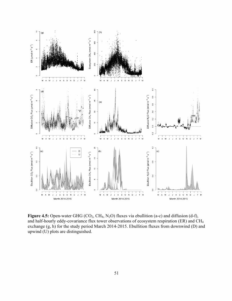
51

Figure 4.5: Open-water GHG (CO2, CH4, N2O) fluxes via ebullition (a-c) and diffusion (d-f), and half-hourly eddy-covariance flux tower observations of ecosystem respiration (ER) and CH4 exchange (g, h) for the study period March 2014-2015. Ebullition fluxes from downwind (D) and upwind (U) plots are distinguished.

52

Table 4.2: Seasonal and annual cumulative GHG flux from diffusive (mean ± S.E), ebullition (Downwind-D vs. Upwind-W; median (Q1-Q3)) and eddy-flux measurements. Season Gas Measurement Spring Summer Fall Winter Annual CO2 Diffusive 186 201 211 317 915 ± 95 g C m-2 Ebullition-D 0.03 0.04 0.04 0.03 0.12 (0.11 – 0.14) Ebullition-U 0.01 0.01 0.03 0.02 0.06 (0.04-0.09) Tower-ER 240 341 268 199 1060 ± 72 CH4 Diffusive 0.38 1.41 0.35 0.21 2.34 ± 0.41 g C m-2 Ebullition-D 0.14 0.68 0.22 0 1.03 (0.78 – 1.36) Ebullition-U 0 0.07 0 0 0.07 (0.03-0.09) Tower-CH4 9.7 24.3 18.2 4.6 57.5 ± 0.84 N2O Diffusive 1,920 60 7,990 52,430 62,400 ± 17,300 µg N m-2 Ebullition-D 7 3 4 13 26 (17-66) Ebullition-U 3 3 5 9 20 (5-102)

4.4.5 Radiative Forcing Effects of Ecosystem GHG Fluxes

Wetland NEE measured at the flux tower was -325 ± 56 g C-CO2 m-2 y-1 and was offset

by CH4 emissions of 57.5 ± 0.84 g C-CH4 m-2 y-1, producing a SGWP of 2.3 ± 0.3 kg CO2-eq m-2 y-1 (Table 3). Tower fluxes, open-water fluxes, and the respective spatial cover fractions (fveg, fwat) were used in a simple mixing model to estimate the parsed vegetation GHG exchange (Sup. Figure 5 and Figure 6). The fveg during summer months (Sup. Figure 5) was very close to independent estimates in past work (~0.63; Matthes et al. 2014) but showed more variability during winter (Table 3; Sup. Figure 5). Parsed annual vegetation NEE and CH4 fluxes were larger than open-water exchanges at -1164 ± 298 g C-CO2 m-2

y-1 and 94.8 ± 12.2 g C-CH4 m-2 y-

1, respectively (Table 3). However, the net warming effect of open-water GHG exchange still exceeded that of vegetated zones (Figure 6). The mixing-model indicated that the SGWP of vegetated zones was 1.4 ± 0.3 kg CO2-eq m-2 y-1, due to high net CO2 uptake (-4.3 ± 1.1 kg CO2 m-2 y-1) offsetting the high CH4 emissions (5.7 ± 0.7 kg CO2-eq m-2 y-1), whereas open-water fluxes of CO2, CH4, and N2O summed to a SWGP of 3.5 ± 0.3 kg CO2-eq m-2 y-1.

Table 4.3: Measured tower and open-water GHG fluxes, mean (± 1SD) annual spatial fractions (fveg, fwat), and model-parsed net GHG fluxes for vegetated zones. Spatial Extent

Fraction (fveg/wat)

NEE (g C m-2 y-1)

CH4 (g C m-2 y-1)

N2O (mg N m-2 y-1)

SGWP (kg CO2-eq m-2 y-1)

Tower variable -325 ± 56 57.5 ± 0.8 - 2.3 ± 0.3 Water 0.40 ± 0.12 915 ± 96 2.9 ± 0.5 62 ± 17 3.5 ± 0.3 Vegetated 0.57 ± 0.12 -1164 ± 298 94.8 ± 12.3 - 1.4 ± 0.4

53

Figure 4.6: Sustained global warming potential (SGWP) of cumulative annual net CO2 and CH4 fluxes measured by the eddy-covariance flux tower (mixed and variable cover type) and separately within open-water and vegetated zones.

After upscaling to spatial extent of vegetation and open water with in the wetland, total annual GHG fluxes were estimated at -379 ± 153 t C-CO2 y-1, 62.3 ± 8.0 t C-CH4 y-1, and 66 ± 18 kg N-N2O y-1, producing an overall wetland radiative forcing effect of 2.4 ± 0.3 kt CO2-eq y-1 over a 100-year time horizon (Table 4). The ecosystem switchover time, which refers to the time horizon for the wetland GHG fluxes to change from a net warming effect to a net cooling effect, was estimated from CO2 uptake to CH4 emission ratios as contributions from N2O were negligible, and GHG fluxes were assumed to be constant over time. Ratios of ~12 and ~6 for vegetation and the entire wetland, respectively, meant that the switchover time for both cover types was > 500 years (Table 4). No switchover time occurs for open-water as long as both CO2 and CH4 fluxes are positive.

4.5 Discussion 4.5.1 Spatial Patterns in Wetland GHG Fluxes & Radiative Forcing

The role of wetland GHG fluxes in global climate change depends on the balance of cooling effects from long-term C sequestration and the warming effects of CH4 and N2O emissions (Frolking and Roulet, 2007; Bridgham et al. 2013; Neubauer and Megonigal, 2015). In

Tower Water Vegetation

Spatial Extent

CH4

NEE

Table 4.4: Wetland zone (vegetated and open-water) spatial extents and associated observed and up-scaled estimates of CO2, CH4, and GHG fluxes. Spatial Extent

Area (m2)

NEE (t C y-1)

CH4 (t C y-1)

N2O (kg N y-1)

SGWP (kt CO2-eq y-1)

CO2:CH4

Switch (y)

Vegetated 644,672 -750 ± 192 61.1 ± 7.9 - 0.9 ± 0.2 ~12 > 500 Water 405,520 371 ± 39 1.3 ± 0.2 25 ± 7 1.4 ± 0.1 - - Wetland 1,050,192 -379 ± 153 62.3 ± 8.0 66 ± 18 2.4 ± 0.3 ~6 > 500

54

the present study high net CH4 emissions from vegetation dominated the radiative forcing effect of a temperate marsh (5.7 kg CO2-eq m-2 y-1), with a much smaller contribution from open-water N2O (0.03 kg CO2-eq m-2 y-1), and a net cooling effect for vegetation uptake of CO2 (-4.3 kg CO2 m-2 y -1). These results support emergent marsh wetlands as particularly large CH4 sources (Whiting and Chanton, 1993; Whalen, 2005; Laanbroek 2010; Bridgham et al. 2013; Knox et al. 2015) and add to a small but growing body of evidence supporting freshwater wetlands as dynamic sources of N2O (Burgin and Groffman, 2012; Moseman-Valtierra, 2012). Our estimates of CO2 uptake (~1.1 kg C-CO2 m-2 y-1) were also comparable to others made at nearby wetlands (Miller and Fujii, 2009; Hatala et al. 2012b; Knox et al. 2015). However unlike other marshes dominated by fast-growing emergent plants (Bridgham et al. 2006), we estimated it would take centuries for CO2 sequestration to offset the warming effects of CH4 release (Neubauer et al. 2015). There is significant uncertainty in estimates of switchover time based on extrapolations from narrows windows of GHG observations, particularly recently after disturbance or restoration, because assumptions must be made about the persistence of fluxes over time. Flux observations at Mayberry since re-flooding in 2010 suggest inter-annual variability can be substantial and that ER will gradually decline over time (Sturtevant et al. 2015) which may lead to greater CO2 sequestration, and reduce ecosystem switchover time. Conversely, GPP may be reduced in emergent marshes following accumulation of dead standing litter, which would further postpone switchover (Anderson et al. 2016). Using multi-year GHG flux observations and modeling of long term GHG dynamics may greatly improve estimates of switchover time. Such approaches have been applied in the context of hydroelectric reservoir creation (Wang et al. 2016) and could be applied similarly to wetlands. It is clear that the expected longevity of restored wetland ecosystems and the persistence of their GHG fluxes are therefore key for understanding the overall climate forcing effects. We also emphasize that the value of wetland restoration cannot be determined by the sole metric of GHG radiative forcing. In the present study, important ecological co-benefits are at stake including habitat restoration, peat soil rebuilding, and levee stabilization (Miller et al. 2011; Moreno-Mateos et al. 2012; Hatala et al. 2012b; Knox et al. 2015; Anderson et al. 2016).

Wetland restoration can optimize ecological and biogeochemical functions by managing hydrologic flow and the distribution of vegetation (Moreno-Mateos et al. 2012). We investigated spatial patterning of open-water and vegetation as drivers of spatial variability in GHG exchange. We found very high net CO2 uptake concentrated in zones of emergent vegetation was strongly offset by high CO2 emissions in open-water. After estimating the SGWP for the two zones separately, we found that open-water emitted more GHG (3.5 kg CO2-eq m-2 y-1) than vegetated areas (1.4 kg CO2-eq m-2 y-1) suggesting that a greater extent of emergent vegetation in some restored wetlands could be favorable from a GHG perspective. This result is surprising given the potential for high CH4 emissions via vegetation in freshwater wetlands, but is likely particular to deep peat wetland soils. The organic C content of wetland soil can regulate the net effect of vegetation on C gas exchange (Laanbroek, 2010), and fermentation and decomposition of deep peat is consistent with a persistent, large, and spatially dispersed source of CO2. It is also possible that the legacy of drainage at the site continues to support elevated rates of CO2 production from underlying peat that may slow down as the site ages (Moreno-Mateos et al. 2012). Furthermore, biogeochemical function in these two wetland zones is connected; C inputs in vegetated zones likely fuel some of the GHG ultimately emitted via open-water pathways. Other connections between these zones include the influence of vegetation canopies on whole-

55

wetland temperature, light-availability, and wind speed. It is clear however that the mix of vegetation and open-water for optimal radiative forcing in restored wetlands will depend on both the current rate of CO2 and CH4 exchange above vegetation as well as the background rate of C gas production from flooded soil, which likely influenced by depth and organic content. 4.5.2 Decoupling of Ebullition & CH4 Content

Spatial patterning of vegetation and open-water also affects the dominant pathways for wetland GHG emission (Bridgham et al. 2013). We used a highly replicated design to estimate open-water ebullition fluxes, a pathway that dominates CH4 release in deeper aquatic environments (Wik et al. 2013) and can bypass oxidation processes even in shallower wetlands (King, 1990). We found low rates of CH4 release via this pathway (~ 1 g C-CH4 m-2 y-1) relative to fluxes from zones of emergent vegetation (94.8 g C-CH4 m-2 y-1). Ebullition fluxes were attenuated by low CH4 content during most of the year. Had CH4 content been fixed at the summer fraction (30 to 50%) year-round ebullition CH4 emissions would have been comparable to emission rates via diffusion (~ 5% of total emissions).

The observed decoupling of ebullition fluxes and CH4 content is surprising given that previous work has shown CH4 content to correlate with ebullition rates (Chanton et al. 1989) and current understanding attributes ebullition bubble growth to excess partial pressure of CH4 in wetland soils (Scandella et al. 2011; Green, 2013). Why did we observe persistent releases of bubble gas along with CH4 content that varied from < 0.01% in winter to > 30% in summer? Back-diffusion from the ebullition chamber headspace into the water column could produce a randomly distributed underestimation of CH4 content on a weekly basis (Varadharajan et al. 2010), and could exhibit some seasonality with lower winter temperatures increasing gas solubility. However, we do not think back-diffusion alone can explain the consistent seasonal variation in content over four orders of magnitude. A possible mechanism is that gases other than CH4 can drive bubble formation outside the growing season. We think this is also unlikely as there is no obvious gas to compensate for lower CH4 production. Dinitrogen (N2) production may vary seasonally due to its redox sensitive production (Davidson and Firestone, 1989), and has very low solubility like CH4 (Sander, 1999). We did observe elevated N2O in winter and higher mineral N concentrations in the adjacent Sacramento River water during winter [EMP discrete water quality data (2015): http://www.water.ca.gov/bdma/reports/] that could support higher rates of denitrification, a source of N2. However, rates of N2 production would have to be unrealistically high to drive the observed rates of ebullition (Chanton et al. 1989; Laanbroek, 2010) outside of treatment wetlands (Zhai et al. 2013). An alternative hypothesis we advance is that the thick layers of sapric peat at the restored wetland facilitated bubble formation at depth, and CH4 was lost during bubble migration to the wetland surface during seasons of low dissolved CH4 (Scandella et al. 2011). The CH4 partial pressure in surficial peat layers is likely to vary seasonally across several orders of magnitude, as was found for surface dissolved CH4. We therefore propose that bubbles retain high CH4 content during migration and release in the summer when high pore-water CH4 is maintained throughout the peat profile. In contrast, when surficial CH4 concentrations are much lower in winter, dissolution and oxidation of CH4 act to strip the bubble of CH4 before ebullitive release. Some studies have found patterns in bubble CH4 content associated with spatial variability in sediment C content, vegetation type, and water depth (Martinez and Anderson, 2013; Wik et al. 2013; Crawford et al. 2014; Hamilton et al.

56

2014). To the best of our knowledge this study is the first to show seasonal decoupling of ebullition rate and CH4 content that acted to attenuate annual CH4 emissions via this pathway. We encourage further work to consider how ebullition gas content may be modulated during migration from deep peat or sediment layers. 4.5.3 Asynchronous Seasonality in Wetland CH4 & N2O

Simultaneous measurement of CO2, CH4 and N2O fluxes can also provide new insights into ecosystem function, especially given the differences in the biogeochemical conditions that facilitate production and consumption. In the present study the observation of strong seasonal asynchronicity between open-water CH4 and N2O inventories (Figure 4) highlights the limitations of simple empirical functions, such as temperature relationships, for interpreting or predicting ecosystem GHG fluxes (Davidson and Janssens, 2006). Enhanced N2O efflux during the cool winter season plainly contradicts an Arrhenius prediction that microbial activity and associated GHG production will scale exponentially with temperature. Rather, both the observed threshold effect and asynchronous dynamics in wetland N2O and CH4 concentrations are consistent with a redox mechanism (Helton et al. 2015). Persistent or fluctuating aerobic conditions favor N2O production and CH4 consumption, whereas persistent anaerobic conditions favor the reverse (Firestone and Davidson, 1989; Hanson and Hanson, 1996). Changing the relative predominance of aerobic and anaerobic zones in wetland soils will therefore strongly favor either N2O or CH4 efflux (McNicol and Silver, 2014), and it follows that our observation of asynchronous CH4 and N2O fluxes that varied seasonally are indicative of ecosystem-scale redox oscillations. High summer temperatures likely increased enzymatic reaction rates and biological O2 demand, driving down redox conditions and favoring the production of reduced gases (CH4 and N2). In contrast, lower winter temperatures likely slowed enzymatic reaction rates and alleviated demand for O2, reoxidizing the wetland soil and favoring oxidized gas species (CO2, N2O). Our data support the kinetic effects of temperature as an intrinsic control of microbial function that are superimposed on, and feedback to, extrinsic controls such as local redox environment of microbial communities (von Fischer and Hedin, 2007; Davidson and Janssens, 2006). 4.6 Conclusions

Our research shows that wetland GHG fluxes are highly dynamic and spatially structured. We used a two-scale approach to quantify annual wetland GHG fluxes and their associated radiative forcing effects, then linked patterns to seasonality, vegetation structure, and transport pathway. The wetland was a net sink for CO2 despite high background rates of CO2 emission measured in the open-water zones. In contrast the wetland was strong source of CH4 with the vast majority emitted from vegetated zones. Although ebullition bubble fluxes were substantial, seasonally low CH4 content reduced the importance of this transport pathway for CH4 emission at the annual timescale. Diffusive CH4 fluxes were of comparable magnitude to those from ebullition, and together represented < 10% of whole ecosystem emissions. The overall SGWP of fluxes highlight the disproportionate role of emergent vegetation on both CO2 uptake and CH4 emission in freshwater wetlands. They also demonstrate that the radiative forcing effect of vegetated zones may be more favorable than open-water when rates of background CO2

57

emissions are high. Though unimportant to wetland radiative forcing, N2O fluxes and their seasonal asynchronicity with CH4 emissions were consistent with wetland redox oscillations as a unifying driver of wetland GHG dynamics. We encourage further work to couple biophysical drivers of plant and microbial function to GHG production, using a framework of redox thermodynamics as the proximate control. 4.7 Supplemental Information

Supplemental Figure 4.7.1: 50% and 80% cumulative footprint contours for DOY 55 2014, 20:00-20:30 hrs, overlaid (inner and outer red ovals, respectively) on classified shape file (black lines) divided into vegetated or open-water zones.

58

Supplemental Figure 4.7.2: Exponential distribution of ebullition flux volumes by season and plot (downwind = grey; upwind = pink).

Supplemental Figure 4.7.3: Seasonal dissolved gas concentration (CO2, CH4, N2O) probability density distributions used for seasonal mean or median flux estimations

Mar−May

Vol (ml m−2 wk−1)

Prob

abilit

y

0 500 1500

0.00

00.

004

DU

Jun−Aug


Prob

abilit

y

0 500 1500

0.00

00.

004

Sep−Nov


Prob

abilit

y

0 500 1500

0.00

00.

004

Dec−Feb


Prob

abilit

y

0 500 1500

0.00

00.

004

Mar−May

CO2 (%)

Prob

abilit

y

0.0 0.6 1.2

02

46

DU

Jun−Aug

CO2 (%)

Prob

abilit

y

0.0 0.6 1.2

02

46

Sep−Nov

CO2 (%)

Prob

abilit

y

0.0 0.6 1.2

02

4

Dec−Feb

CO2 (%)

Prob

abilit

y

0.0 0.6 1.2

02

4

CH4 (ppm(v))

Prob

abilit

y

0 1000

0.00

CH4 (ppm(v))

Prob

abilit

y

0 10000.00

00.

002

CH4 (ppm(v))

Prob

abilit

y

0 10000.00

00.

009

CH4 (ppm(v))

Prob

abilit

y

0 10000.00

00.

006

N2O (ppb(v))

Prob

abilit

y

0 1200 30000.00

00.

004

N2O (ppb(v))

Prob

abilit

y

0 1200 30000.00

00.

004

N2O (ppb(v))

Prob

abilit

y

0 1200 30000.00

00.

004

N2O (ppb(v)

Prob

abilit

y

0 1200 30000.00

00.

004

59

Supplemental Figure 4.7.4: Seasonal ebullition gas concentration (CO2, CH4, N2O) probability density distributions used for seasonal mean or median flux estimations

Supplemental Figure 4.7.5: Fractions of vegetation (fveg) and open water (fwat) estimated from flux footprint overlay on cover type classification shapefile.

Mar−May

CO2 (%)Pr

obab

ility

0 2 4

0.0

1.0

2.0 D

U

Jun−Aug

CO2 (%)

Prob

abilit

y

0 2 4

0.0

0.4

0.8

Sep−Nov

CO2 (%)

Prob

abilit

y

0 2 4

0.0

0.4

0.8 Dec−Feb

CO2 (%)

Prob

abilit

y

0 2 4

0.0

0.4

0.8

CH4 (%)

Prob

abilit

y

0.001 1 100

0.0

0.4

0.8

CH4 (%)Pr

obab

ility

0.001 1 100

0.0

0.6

1.2

CH4 (%)

Prob

abilit

y

0.001 1 100

0.0

0.4

0.8

CH4 (%)

Prob

abilit

y

0.001 1 100

0.0

0.4

0.8

1.2

N2O (ppm(v))

Prob

abilit

y

0.01 1 100

0.0

1.0

2.0

N2O (ppm(v))

Prob

abilit

y

0.01 1 100

0.0

0.6

1.2

N2O (ppm(v))Pr

obab

ility

0.01 1 100

0.0

0.4

0.8

N2O (ppm(v))

Prob

abilit

y

0.01 1 100

0.0

0.6

1.2

60

Supplemental Figure 4.7.6: Parsed vegetation net CO2 (NEE) and CH4 exchange from tower fluxes, open-water flux observations, and the respective cover type fractions each sampling period 5.8 Acknowledgements

We thank Jackson Chin, Heather Dang, Ryan Saladay, and Laura Southworth for assistance with field data collection. Whendee Silver, Dennis Baldocchi, Iryna Dronova, Sara Knox, and Cove Sturtevant contributed to the writing of this chapter. We are also grateful for advice from Charuleka Varadharajan on adapting ebullition flux chamber designs. This research was supported by the Delta Science Program grant (#2053) and an NSF Doctoral Dissertation Improvement Grant (DEB-1405715). This research was also supported by the USDA National Institute of Food and Agriculture McIntire Stennis project CA-B-ECO-7673-MS 450 to W. Silver. GM was also supported as a Lawrence Graduate Scholar at Lawrence Livermore National Laboratory and as a Research Fellow of the University of California Carbon Neutrality Initiative.

GM and WS designed the study, GM conducted the chamber sampling while SK, CS, and DD oversaw and processed eddy-covariance flux observations. ID contracted the remote sensing imagery and conducted the spatial classification (supported by the Delta Science Program grant #R/SF-52 and Geospatial Innovation Facility at UC Berkeley, gif.berkeley.edu), CS developed the R code for spatial fraction estimation, and GM authored the manuscript. 5.9 References

61

Anderson FE, Bergamaschi BA, Sturtevant C et al. (2016) Variation of energy and carbon fluxes from a restored temperate freshwater wetland and implications for carbon market verification protocols. Journal of Geophysical Research Biogeosciences, 121. Armstrong W, Armstrong J, Beckett PM, Justin SHFW (1991) Convective gas-flows in wetland plant aeration. In: Plant life under oxygen deprivation. Ecology, Physiology and biochemistry. (eds Jackson MB, Davies DD, Lambers H) pp Page. The Hague, SPB Academic. Baldocchi DD, Hincks BB, Meyers TP (1988) Measuring biosphere-atmosphere exchanges of biologically related gases with micrometeorological methods. Ecology, 69, 1331-1340. Baldocchi DD (2003) Assessing the eddy covariance technique for evaluating carbon dioxide exchange rates of ecosystems: past, present and future. Glob Chang Biol, 9, 1-14. Baldocchi D, Sturtevant C, Contributors F (2015) Does day and night sampling reduce spurious correlation between canopy photosynthesis and ecosystem respiration? Agricultural and Forest Meteorology, 207, 117-126. Beaulieu JJ, Nietch CT, Young JL (2015) Controls on nitrous oxide production and consumption in reservoirs of the Ohio River Basin. Journal of Geophysical Research: Biogeosciences, 120, 1995-2010. Benz UC, Hofmann P, Willhauck G, Lingenfelder I, Heynen M (2004) Multi-resolution, object-oriented fuzzy analysis of remote sensing data for GIS-ready information. ISPRS Journal of Photogrammetry and Remote Sensing, 58, 239-258. Blaschke T (2010) Object based image analysis for remote sensing. ISPRS Journal of Photogrammetry and Remote Sensing, 65, 2-16. Bridgham SD, Cadillo-Quiroz H, Keller JK, Zhuang Q (2013) Methane emissions from wetlands: biogeochemical, microbial, and modeling perspectives from local to global scales. Glob Chang Biol, 19, 1325-1346. Bridgham SD, Megonigal JP, Keller JK, Bliss NB, Trettin C (2006) The carbon balance of North American wetlands. Wetlands, 26, 889-916. Burgin AJ, Groffman PM (2012) Soil O2 controls denitrification rates and N2O yield in a riparian wetland. J Geophys Res, 117, doi:10.1029/2011JG001799. Chanton JP, Martens CS, Kelley CA (1989) Gas transport from methane-saturated, tidal freshwater and wetland sediments. Limnol Oceanogr, 34, 807-819. Cole JJ, Caraco NF (1998) Atmospheric exchange of carbon dioxide in a low-wind oligotrophic lake measured by the addition of SF6. Limnol Oceanogr, 43, 646-656.

62

Cole JJ, Bade DL, Bastviken D, Pace ML, Van De Bogert M (2010) Multiple approaches to estimating air-water gas exchange in small lakes. Limnology and Oceanography: Methods, 8, 285-293. Conrad R (1996) Soil microorganisms as controllers of atmospheric trace gases (H2, CO, CH4, OCS, N2O, and NO). Microbiological Reviews, 60, 609-640. Crawford JT, Stanley EH, Spawn SA, Finlay JC, Loken LC, Striegl RG (2014) Ebullitive methane emissions from oxygenated wetland streams. Glob Chang Biol, 20, 3408-3422. Cui S, Shi Y, Groffman PM, Schlesinger WH, Zhu Y-G (2013) Centennial-scale analysis of the creation and fate of reactive nitrogen in China (1910-2010). Proc Natl Acad Sci U S A, 110, 2052-2057. Davidson EA, Samanta S, Caramori SS, Savage K (2012) The Dual Arrhenius and Michaelis-Menten kinetics model for decomposition of soil organic matter at hourly to seasonal time scales. Glob Chang Biol, 18, 371-384. Davidson EA, Savage KE, Finzi AC (2014) A big-microsite framework for soil carbon modeling. Glob Chang Biol, 20, 3610-3620. Detto M, Montaldo N, Albertson JD, Mancini M, Katul G (2006) Soil moisture and vegetation controls on evapotranspiration in a heterogeneous Mediterranean ecosystem on Sardinia, Italy. Water Resources Research, 42. Detto M, Verfaillie J, Anderson F, Xu L, Baldocchi D (2011) Comparing laser-based open- and closed-path gas analyzers to measure methane fluxes using the eddy covariance method. Agricultural and Forest Meteorology, 151, 1312-1324. Drexler JZ, De Fontaine CS, Brown TA (2009a) Peat accretion histories during the past 6,000 years in marshes of the Sacramento-San Joaquin Delta, CA, USA. Estuaries and Coasts, 32, 871-892. Drexler JZ, De Fontaine CS, Deverel SJ (2009b) The legacy of wetland drainage on the remaining peat in the Sacramento-San Joaquin Delta, California, USA. Wetlands, 29, 372-386. Dronova I (2015) Object-Based Image Analysis in Wetland Research: A Review. Remote Sensing, 7, 6380-6413. Falkowski PG, Fenchell T, Delong EF (2008) The microbial engines that drive Earth's biogeochemical cycles. Science, 320, 1034-1039. Firestone MK, Davidson EA (1989) Microbiological basis of NO and N2O Production and Consumption. In: Exchange of Trace Gases between Terrestrial Ecosystems and the Atmosphere. (eds Andreae MO, Schimel DS) pp Page. Chichester, UK, John Wiley & Sons Ltd.

63

Freeman C, Ostle NJ, Kang H (2001) An enzymatic 'latch' on a global carbon store. Nature, 409, 149. Green SM (2013) Ebullition of methane from rice paddies: the importance of furthering understanding. Plant and Soil, 370, 31-34. Hall SJ, McDowell WH, Silver WL (2012) When wet gets wetter: Decoupling of moisture, redox biogeochemistry, and greenhouse gas fluxes in a humid tropical forest soil. Ecosystems, 16, 576-589. Hatala JA, Detto M, Baldocchi DD (2012a) Gross ecosystem photosynthesis causes a diurnal pattern in methane emission from rice. Geophysical Research Letters, 39. Hatala JA, Detto M, Sonnentag O, Deverel SJ, Verfaillie J, Baldocchi DD (2012b) Greenhouse gas (CO2, CH4, H2O) fluxes from drained and flooded agricultural peatlands in the Sacramento-San Joaquin Delta. Agriculture, Ecosystems & Environment, 150, 1-18. Hamilton S, Sippel S, Chanton J, Melack J (2014) Plant-mediated transport and isotopic composition of methane from shallow tropical wetlands. Inland Waters, 4, 369-376. Helton AM, Ardon M, Bernhardt ES (2015) Thermodynamic constraints on the utility of ecological stoichiometry for explaining global biogeochemical patterns. Ecol Lett, 18, 1049-1056. Hsieh CI, Katul G, Chi T (2000) An approximate analytical model for footprint estimation of scalar fluxes in thermally stratified atmospheric flows. Advances in Water Resources, 23, 765-777. IPCC (2013) Summary for Policymakers. In: Climate Change 2013: The Physical Science Basis. Contribution of Working Group I to the Fifth Assessment Report of the Intergovernmental Panel on Climate Change. (eds Stocker TF, Qin D, Plattner G-K, Tignor M, Allen SK, Boschung J, Nauels A, Xia Y, Bex V, Midgley PM) pp Page. Cambridge, United Kingdom and New York, NY, USA, Cambridge University Press. Jungkunst HF, Fiedler S (2007) Latitudinal differentiated water table control of carbon dioxide, methane and nitrous oxide fluxes from hydromorphic soils: feedbacks to climate change. Glob Chang Biol, 13, 2668-2683. Knox SH, Sturtevant C, Matthes JH, Koteen L, Verfaillie J, Baldocchi D (2015) Agricultural peatland restoration: effects of land‐use change on greenhouse gas (CO2 and CH4) fluxes in the Sacramento‐San Joaquin Delta. Glob Chang Biol, 21, 750-765. Knox SH, Matthes JH, Sturtevant C, Oikawa P, Verfaillie J, Baldocchi D (2016) Photosynthesis and soil temperature regulate interannual variability in ecosystem scale methane emissions from a California rice paddy. Journal of Geophysical Research – Biogeosciences. Accepted.

64

Koebsch F, Jurasinski G, Koch M, Hofmann J, Glatzel S (2015) Controls for multi-scale temporal variation in ecosystem methane exchange during the growing season of a permanently inundated fen. Agricultural and Forest Meteorology, 204, 94-105. Laanbroek HJ (2010) Methane emission from natural wetlands: interplay between emergent macrophytes and soil microbial processes. A mini-review. Ann Bot, 105, 141-153. Limpens J, Berendse F, Blodau C et al. (2008) Peatlands and the carbon cycle: from local processes to global implications - a synthesis. Biogeosciences, 5, 1475-1491. Martinez D, Anderson MA (2013) Methane production and ebullition in a shallow, artificially aerated, eutrophic temperate lake (Lake Elsinore, CA). Sci Total Environ, 454-455, 457-465. Matthes JH, Sturtevant C, Verfaillie J, Knox S, Baldocchi D (2014) Parsing the variability in CH4 flux at a spatially heterogeneous wetland: Integrating multiple eddy covariance towers with high-resolution flux footprint analysis. Journal of Geophysical Research: Biogeosciences, 119, 1322-1339. Matthews E, Fung I (1987) Methane emission from natural wetlands: Global distribution, area, and environmental characteristics of sources. Global Biogeochemical Cycles, 1, 61-86. Matthews CJ, St. Louis VL, Hesslein RH (2003) Comparison of three techniques used to measure diffusive gas exchange from sheltered aquatic surfaces. Environ Sci Technol, 37, 772-780. McNicol G, Silver WL (2014) Separate effects of flooding and anaerobiosis on soil greenhouse gas emissions and redox sensitive biogeochemistry. Journal of Geophysical Research: Biogeosciences, 119, 557-566. Megonigal JP, Hines ME, Visscher PT (2004) Anaerobic metabolism: Linkages to trace gases and aerobic processes. In: Biogeochemistry, Treatise on Geochemistry. (ed Schlesinger WH) pp 317-424. Oxford, UK, Elsevier-Pergamon. Mitsch WJ, Gosselink JG (2015) Wetlands of the world. In: Wetlands, 5th edn. pp 45-110. New York, USA, John Wiley & Sons. Mitsch WJ, Zhang L, Stefanik KC et al. (2012) Creating Wetlands: Primary Succession, Water Quality Changes, and Self-Design over 15 Years. BioScience, 62, 237-250. Moreno-Mateos D, Power ME, Comin FA, Yockteng R (2012) Structural and functional loss in restored wetland ecosystems. PLoS Biol, 10, e1001247. Moseman-Valtierra S (2012) Reconsidering the climatic role of marshes: Are they sinks or sources of greenhouse gases. In: Marshes: ecology, management and conservation. pp 1-48. Hauppauge, Nova Scientific Publishers.

65

Neubauer SC (2014) On the challenges of modeling the net radiative forcing of wetlands: reconsidering Mitsch et al. 2013. Lanscape Ecol, 29, 571-577. Neubauer SC, Megonigal JP (2015) Moving beyond global warming potentials to quantify the climatic role of ecosystems. Ecosystems, 18, 1000-1013. Oikawa PY, Grantz DA, Chatterjee A, Eberwein JE, Allsman LA, Jenerette GD (2014) Unifying soil respiration pulses, inhibition, and temperature hysteresis through dynamics of labile soil carbon and O2. Journal of Geophysical Research Biogeosciences, 119, 521-536. Pett-Ridge J, Firestone MK (2005) Redox fluctuation structures microbial communities in a wet tropical soil. Applied and Environmental Microbiology, 71, 6998-7007. Peters V, Conrad R (1996) Sequential reduction processes and initiation of CH4 production upon flooding of oxic upland soils. Soil Biology and Biochemistry, 28, 371-382. Poindexter CM, Variano EA (2013) Gas exchange in wetlands with emergent vegetation: The effects of wind and thermal convection at the air-water interface. Journal of Geophysical Research: Biogeosciences, 118, 1297-1306. Sander R (2015) Compilation of Henry's law constants (version 4.0) for water as solvent. Atmospheric Chemistry and Physics, 15, 4399-4981. Scandella BP, Varadharajan C, Hemond HF, Ruppel C, Juanes R (2011) A conduit dilation model of methane venting from lake sediments. Geophysical Research Letters, 38, doi:10.1029/2011gl046768. Sietzinger S, Harrison JA, Böhlke JK, Bouwman AF, Lowrance R, Peterson B, Tobias C, Drecht GV (2006) Denitrification across landscapes and waterscapes: A synthesis. Ecological Applications, 16, 2064-2090. Stefanik KC, Mitsch WJ (2014) Metabolism and methane flux of dominant macrophyte communities in created riverine wetlands using open system flow through chambers. Ecological Engineering, 72, 67-73. Stoy PC, Mauder M, Foken T et al. (2013) A data-driven analysis of energy balance closure across FLUXNET research sites: The role of landscape scale heterogeneity. Agricultural and Forest Meteorology, 171-172, 137-152. Stull RB (2012) Similarity Theory. In: An introduction to boundary layer meteorology. pp 385. Berlin, Germany, Springer Science & Business Media. Sturtevant C, Ruddell BL, Knox SH, Verfaillie J, Matthes JH, Oikawa PY, Baldocchi D (2016) Identifying scale-emergent, nonlinear, asynchronous processes of wetland methane exchange. Journal of Geophysical Research: Biogeosciences, 121.

66

Takai Y, Kamura T (1966) The mechanism of reduction in waterlogged paddy soil. Folia Microbiologica, 11, 304-313. Teh YA, Silver WL, Sonnentag O, Detto M, Kelly M, Baldocchi DD (2011) Large greenhouse gas emissions from a temperate peatland pasture. Ecosystems, 14, 311-325. Tokida T, Cheng W, Adachi M, Matsunami T, Nakamura H, Okada M, Hasegawa T (2012) The contribution of entrapped gas bubbles to the soil methane pool and their role in methane emission from rice paddy soil in free-air [CO2] enrichment and soil warming experiments. Plant and Soil, 364, 131-143. Varadharajan C, Hermosillo R, Hemond HF (2010) A low-cost automated trap to measure bubbling gas fluxes. Limnol Oceanogr-meth, 8, 363-375. Vartapetian BB, Jackson MB (1996) Plant adaptations to anaerobic stress. Annals of Botany, 79, 3-20. Venkiteswaran JJ, Rosamond MS, Schiff SL (2014) Nonlinear response of riverine N2O fluxes to oxygen and temperature. Environ Sci Technol, 48, 1566-1573. Von Fischer JC, Hedin LO (2007) Controls on soil methane fluxes: Tests of biophysical mechanisms using stable isotope tracers. Global Biogeochemical Cycles, 21. Wang W, Roulet NT, Kim Y, Strachan IB, Del Giorgio P, Prairie YT, Tremblay A (2016) Integrating aquatic and terrestrial biogeochemical model to predict effects of reservoir creation on CO2 emissions. Biogeosciences Discussions, 1-33. Weston NB, Neubauer SC, Velinsky DJ, Vile MA (2014) Net ecosystem carbon exchange and the greenhouse gas balance of tidal marshes along an estuarine salinity gradient. Biogeochemistry, 120, 163-189. Whalen SC (2005) Biogeochemistry of methane exchange between natural wetlands and the atmosphere. Environmental Engineering Science, 22, 73-94. Whiting GJ, Chanton JP (1993) Primary production control of methane emission from wetlands. Nature, 364, 794-795. Wik M, Crill PM, Varner RK, Bastviken D (2013) Multiyear measurements of ebullitive methane flux from three subarctic lakes. Journal of Geophysical Research: Biogeosciences, 118, 1307-1321. Wik M, Thornton BF, Bastviken D, Uhlbäck J, Crill PM (2016) Biased sampling of methane release from northern lakes: A problem for extrapolation. Geophysical Research Letters, 43, doi:10.1002/2015GL066501.

67

Wilson K, Goldstein A, Falge E, Aubinet M, Baldocchi D (2002) Energy balance closure at FLUXNET sites. Agricultural and Forest Meteorology, 113, 223-243. Yvon-Durocher G, Allen AP, Bastviken D et al. (2014) Methane fluxes show consistent temperature dependence across microbial to ecosystem scales. Nature, 507, 488-491. Zedler JB, Kercher S (2005) Wetland resources: Status, trends, ecosystem services, and restorability. Annu Rev Environ Resour, 30, 39-74. Zhai X, Piwpuan N, Arias CA, Headley T, Brix H (2013) Can root exudates from emergent wetland plants fuel denitrification in subsurface flow constructed wetland systems? Ecological Engineering, 61, 555-563.

68

Chapter 5: Radiocarbon reveals dynamic contributions from recent photosynthesis and bulk peat carbon to decomposition in a restored wetland

‘Homer was wrong’ wrote Hercleitus of Ephesus. ‘Homer was wrong in saying: “Would that strife would perish from among Gods and men”.

He did not see that he was praying for the destruction of the universe; for if his prayer was heard, all things would pass away.’

- Aldous Huxley [1928] 5.1 Abstract

Wetlands play an important role in the global carbon cycle and climate system by sequestering atmospheric carbon dioxide and emitting methane. The turnover of recently fixed and bulk soil carbon pools regulate the balance of these fluxes in wetlands and determine their overall climate effects. Wetland restoration on drained peatland soil aims to re-stabilize bulk peat carbon and slow decomposition, but no studies to date have distinguished the carbon sources for decomposition to evaluate the effects of restoration. We used the radiocarbon isotopic composition (∆14C) of sediment gas bubbles, plant stem emissions, and the soil profile in a restored emergent marsh to determine contributions of recently fixed and bulk peat to carbon dioxide and methane emissions. We found that a substantial (30 to 50%) fraction of wetland decomposition products are derived from bulk peat carbon sources after 4 to 5 years of permanent inundation. We also found that the fraction of decomposition products derived from each source is relatively aseasonal, despite highly seasonal carbon inputs and seasonality in absolute emissions when source fractions were coupled with spatially parsed gas fluxes. Emergent vegetation stimulated both methane and carbon dioxide production via the products of annual photosynthesis against a background of older peat decomposition. Monthly sampling over a year showed that physical transport by plants also enhanced wetland gas emission, varying with seasonal cycles. Our combined radiocarbon and gas flux approach shows significant losses of C derived from bulk peat sources in a restored wetland and demonstrates the ecological links between wetland structure, seasonality, and carbon cycling. 5.2 Introduction

Wetlands can sequester atmospheric carbon dioxide (CO2) over long time scales, and collectively they store the majority of soil carbon (C) globally (Limpens et al. 2008). However, wetlands are also the largest natural source of methane (CH4), a significantly more potent greenhouse gas (Bridgham et al. 2006; IPCC, 2013). Relatively low rates of CH4 emission can therefore offset net ecosystem C gains via primary production (Neubauer and Megonigal, 2015), and may form a positive feedback to global warming (Yvon-Durocher et al. 2014). The balance between C uptake and C release as CO2 or CH4 is influenced by climate, vegetation, and soil biogeochemistry. However, how these factors interact in situ to regulate this balance is still poorly understood (Bridgham et al. 2013).

69

Carbon emissions from wetlands are sourced from a combination of fresh, labile C inputs from actively growing plants and from the slower breakdown of older, stored organic matter in wetland sediment and peat. Annual plant C fixation is generally thought to provide most of the substrates for wetland decomposition; this is supported by observed correlations between ecosystem gross primary productivity (GPP) and annual wetland CH4 emissions at coarse spatial scales (Whiting and Chanton, 1993). However, GPP is also typically correlated with temperature in wetlands, and may mask dynamic contributions from bulk peat C sources that can also respond to temperature variation (Bosatta and Ågren, 1999; Davidson and Janssens, 2006; von Lützow and Kögel-Knabner, 2009).

Radiocarbon (14C) measurements can be used to differentiate the C sources of CH4 emissions from wetlands. 14C is advantageous as a natural tracer because 13C corrections during ∆14C calculation eliminate isotopic fractionation effects that confound the interpretation of stable (δ13C) isotopic signatures (Stuiver and Polach, 1977; Whiticar, 1999). However, as with other isotope tracers, 14C provides clearest insights when different source substrates carry strongly distinctive isotopic signatures (Wanatabe and Kuwae, 2015). It therefore is a promising approach to investigate C cycling in wetlands where upper soil, or peat, horizons have been lost due to oxidation during periodic drying or managed drainage. Here the contrast in 14C content between contemporary atmospheric CO2, entering the ecosystem annually via photosynthesis, and the remaining bulk peat C, is much greater, and may permit the clearer distinction of these different C sources. Furthermore, the stability of different C pools in re-flooded peatlands and wetlands is a key biogeochemical metric to measure the success of restoration (Mitsch et al. 2012; Moreno-Mateos, 2012), and must be better understood to successfully restore a persistent C sink in these ecosystems (Hatala et al. 2012; Knox et al. 2016; Anderson et al. 2016).

A handful of studies have used 14C observations of CO2 and CH4 to identify source substrates (Lassey et al. 2007), including the contribution of recently fixed photosynthetic C that carries the modern ∆14C signature of atmospheric CO2 (Quay et al. 1988; Chanton et al. 1995; Bellisario et al. 1999; Nakagawa et al. 2002; Garnett et al. 2012). With the exception of Garnett et al. (2012), these studies have consistently observed modern 14C signatures and infer that wetland C gas release is primarily driven by plant inputs of photosynthetic C, which turns over on annual or decadal timescales. There are, however, some limitations of these data. First, bulk soil C contributions to wetland CO2 and CH4 are likely to be derived from decomposing surface soil or peat horizons – decades to centuries old - where oxygen and other biogeochemical gradients are steepest (Clymo and Pierce, 1995; Shoemaker and Schrag, 2010). These same layers are likely to differ only slightly in their 14C signature from contemporary atmospheric (modern) C due to the vertical accretion of wetland soils, and therefore the bulk C signal may be obscured. Second, wetland 14C work thus far has drawn conclusions from the 14C signature itself, which only provides a relative description of C sources. However, wetland CO2 and CH4 production and emissions tend to vary in time and space, meaning the same modern 14C signature measured at different times or places - when fluxes differ - may mask dynamic contributions from older, bulk soil C sources. Lastly, conclusions have been drawn from studies conducted almost entirely in high latitude, rainfed, peatbogs (Martens et al. 1992; Chanton et al. 1995; Bellisario et al. 1999; Garnett et al. 2012), where background rates of respiration are particularly low due to phenolic accumulation (Freeman et al. 2001; Freeman et al. 2004; Sinsabaugh 2010). Much less work has been conducted in nutrient-rich fens or emergent marshes

70

in temperate or tropical zones where warmer temperatures and greater inputs of C could interact to make both plant and bulk soil C sources important to wetland CO2 and CH4 dynamics (Kirschke et al. 2013). Distinguishing these different C sources is key for understanding the role of vegetation on gas exchange, determining the residence time of photosynthetic C in wetlands, and predicting how wetland C exchange will respond to changes in temperature and plant productivity under future climate change.

Figure 5.1: Distinguishing physical ‘straw’ and biological ‘stimulant’ effects of emergent wetland plants. The physical effects (left) arise as emergent plants provide a gas-phase conduit for emission, sometimes enhanced by convective gradients, and can rapidly transport sediment gases including CO2 and CH4 to the atmosphere. The biological effects (right) arise due to the interaction of rhizome exudation and proximate microbial communities and include stimulation of CO2 and CH4 production from root organic C (Org C) and CH4 oxidation from radial O2 loss.

Emergent vegetation, in particular, influences many C cycle processes in wetlands (Laanbroek, 2010), often dominating CO2 uptake via photosynthesis, providing substrates for decomposition, and acting as a physical conduit for CH4 emission (Box 1). There has been considerable research directed at identifying specific ecological interactions between wetland plants and soil microbes, and their effect on C gas exchange (Armstrong, 1979; King, 1990; Chanton et al. 1993; King, 1996; Minoda et al. 1996; Jackson and Armstrong, 1999 Sutton-Grier and Megonigal, 2011). Labile organic C substrates from root exudation and sloughing can be degraded to hydrogen gas (H2), acetate, and CO2, which are the precursors of CH4 production (Minoda et al. 1996) or may stimulate decomposition generally via priming mechanisms (Fontaine et al. 2003; Blagodatskya, 2010). Simultaneously, oxygen (O2) leaking radially from roots can stimulate aerobic CH4 oxidation (King, 1996) or may lead to the competitive inhibition of CH4 production by regenerating alternative electron acceptors, such as ferric iron (Sutton-

71

Grier and Megonigal, 2011). In addition to biological stimulation effects, emergent plants have physical effects on wetland gas exchange. The lacunar structure of emergent macrophytes (aerenchyma) facilitates gas circulation between the atmosphere and inundated rhizomes, ventilating sediments of poorly soluble gases such as CH4 (Armstrong, 1979; Jackson and Armstrong, 1999). Moreover, some ubiquitous species, such as Schoenplectus spp. and Typha spp. that often rapidly colonize restored or disturbed wetlands, use stomatal regulation to advect gases from the rhizosphere, further enhancing emission and bypassing water-column CH4 consumption (King, 1990; Chanton et al. 1993). Other interesting synergies between rhizome gas circulation and CH4 production can emerge where the latter may be stimulated by a change in the steady-state concentration of CH4 via gas removal (Shoemaker and Schrag, 2010; Blodau, 2011), as is facilitated by emergent plant stems.

In the present study we use 14C as a natural tracer in a restored temperate emergent wetland to distinguish the relative importance of recently fixed photosynthetic C and bulk peat C as substrate sources driving heterotrophic CO2 and CH4 production. We exploit the strong 14C isotopic contrast between modern atmospheric CO2 entering via plant photosynthesis, and the old layers of degraded peat. By using spatially stratified monthly sampling of sediment and plant stem gas over a year we investigated three main questions: (1) Does older bulk peat C continue to contribute to CO2 and CH4 emissions after wetland re-establishment? (2) How do spatial structure and seasonality in ecosystem production regulate contributions from each C source? (3) Does the presence of emergent vegetation increase gas emissions primarily via a physical transport effect or a biological stimulation effect? 5.3 Method 5.3.1 Study Site & Design

The study was carried out at Mayberry Farms (38.0498°N 121.6469°W), a restored wetland located on Sherman Island in the Sacramento Delta, California. The Delta’s climate is Mediterranean characterized by cool wet winters and hot dry summers. Average temperatures range from 7.9 ˚C in January to 24.1 ˚C in July, and mean annual precipitation is 336 mm (1981-2010, local meteorological data, Antioch, CA).

The site exhibits a strong 14C contrast between surficial peat layers and contemporary atmospheric CO2. The 14C contrast is a legacy of levee construction and peatland reclamation that allowed for drained agriculture in the Delta over the last century. Rapid oxidation and compaction of drained peat layers caused Sherman Island to subside by >4 m relative to sea level and has left a partially oxidized peat horizon of ~ 1 m overlaying 1-2 m of intact peat (Drexler et al. 2009a). Mayberry was restored to a wetland in October 2010 (Knox et al. 2015) and surface organic matter is therefore older (> 3000 yr BP; Drexler et al. 2009b) and much more depleted in ∆14C than the surface horizons of intact wetland or peatland soils. Current photosynthetic inputs of C therefore introduce 14C that is highly enriched (more modern) relative to bulk soil organic matter, which we traced to understand variability in the C substrates driving CO2 and CH4 emissions.

72

The site also displays distinct spatial patterning of open-water and dense emergent vegetation and strong seasonality in ecosystem production (Matthes et al. 2014). The wetland was designed to feature variable bathymetry, with both shallow (10-30 cm) and deep (1-2 m) water. Since 2010, dense patches of 2-3 m tall emergent Typha and Schoenoplectus spp. have grown in the shallow water areas, while deeper areas remain open-water zones (Matthes et al. 2014; Knox et al. 2015). Past work at the site has demonstrated the primary importance of emergent vegetation for CO2 uptake and CH4 emission. Furthermore, ecosystem production at Mayberry is highly seasonal, with most of the ~1 kg C-CO2 m-2 yr-1 of gross productivity occurring during the summer growing season (March – September; Knox et al. 2015). Mayberry exhibits strong spatial and temporal structure in the inputs of photosynthetic C that we explored as drivers of C gas flux dynamics. 5.3.2 Field Sample Collection

Wetland sediment gas samples in both vegetated and open-water zones were collected monthly from February 14, 2014 to February 13, 2015. Gas was collected manually by stimulating small ebullition events and trapping the emitted gas in a custom-built ebullition chamber (Varadharajan et al. 2010) before they reached the water-surface. Ebullition was stimulated by gentle perturbation of surficial wetland sediment to a depth of approximately 10 cm using a meter stick. At least 90 ml of gas was collected to ensure sufficient molar quantities (> 25 µmol C) of CO2 and CH4 for subsequent analyses. Insufficient gas was collected for ∆14CO2 analysis from the open-water plots on the first sampling date (February 14, 2014) and for δ 13CO2 analysis from February to November 2014 due to lower than expected CO2 concentrations.

Gas emitted directly via emergent plant (Typha) stems was collected monthly during the growing season between April and September 2014. Stems were clipped at ~10 cm above the water surface before being enclosed within a cylindrical PVC flux chamber (30 cm H x 25 cm D), adapted to float by securing a polystyrene ring to the chamber base. Between one and four stems were clipped and enclosed each time, representing a mixture of growing and senesced tissue. Five 30 ml headspace subsamples were taken at recorded times over 40 minutes using a syringe and injected into pre-evacuated 20 ml glass vials (over-pressurized) for CH4 concentration analyses. These data ensured that ebullition gas releases did not occur during sampling, which would artificially increase the headspace gas concentrations. After ~ 45 min, the entire chamber headspace volume was pumped into a 10 L aluminum foil gas sampling bag (Restek®, Bellefonte, PA, United States) using battery powered diaphragm pump (KNF Neuberger, Inc., Trenton, NJ, United States). We avoided producing a vacuum within the 14 L chamber during gas removal (8-10 L) by allowing ambient atmosphere to enter via a needle inserted into the sampling port. Additional gas samples were collected from the gasbag immediately after pumping, and later alongside gas analyses, to check for significant dilution or leaking.

Peat underlying the restored wetland was also characterized as the bulk soil C end-member for decomposition. The peaty soils were sampled on May 15, 2015 at the triplicate vegetated and open-water plots used for gas collection. A soil augur was used to collect cores at 10 cm increments from 0-50 cm deep in the profile for a total of 30 samples. Visually

73

identifiable surface material and plant detritus was removed from cores before they were sealed in plastic storage bags (Ziploc™) and transported back to UC Berkeley (UCB) in a cooler where they air-dried at room temperature (~24 °C) for 4-6 weeks. Once dry, soil was sieved (2 mm) and ground to a fine powder; 1-2 mg was subsampled for total C on a CN elemental analyzer (CE Elantech, Lakewood, NJ, United States). Remaining samples were transported to the Center for Accelerator Mass Spectrometry (CAMS) at Lawrence Livermore National Laboratory (LLNL) for isotopic analyses. 5.3.3 Gas & Isotope Analyses

Subsamples (5 ml) of sediment and plant stem gas were analyzed at UCB on a Shimadzu GC-14A (Shimadzu Scientific Inc., Columbia, MD, USA) for CO2 and CH4 concentrations using thermal conductivity and flame ionization detectors, respectively. A standard gas containing 997 ppm(v) CO2 and 9.91 ppm(v) CH4 (Praxair Inc., Los Angeles, CA, USA) was run alongside samples to calibrate unknowns in 101-103 ppm(v) range. Run precision was always < 2%, calculated as the coefficient of variance on replicate standards. A high-CH4 standard (99.0%; Restek®, Bellefonte, PA, USA) was used for calibration with sediment gas samples that typically contained percent-range CH4 concentrations and were run at lower detector sensitivity. Plant stem samples were screened for contaminating ebullition events by checking for large spikes in the initial (0-45 min) gas time series; however, no samples were removed on this basis.

Sediment and plant stem gas samples were purified to isolate CH4 and CO2 (sediment gas only) for stable C (δ13C) and ∆14C isotope analyses on a newly built cryogenic extraction line at CAMS LLNL. Vacuum line design was based on Petrenko et al. (2008). Sample was introduced to the vacuum line at ambient pressure. The 10 L gasbag samples from plant stems were directly introduced to the vacuum line via a 19-gauge needle port while the sediment gas vial samples were first combined in a single 1 L gasbag then diluted in a 5 L gasbag to 102-103 ppm(v) range with ultra zero-air (19.5–23.5% O2, balance N2; Air Liquide America Specialty Gases LLC, Plumsterdville, PA, USA). Sample gas was passed through a dry-ice trap, Sofnocat™ (Molecular Products Ltd. Thaxton, Essex, UK) catalyst, and three Russian-doll liquid N2 (LN) traps that removed H2O, CO, and CO2. Remaining gas constituents were then CH4, N2, O2, Ar and other trace non-condensing gases. At this point the sample passed through a combustion furnace set to 780 °C and containing a platinized quartz-wool catalyst (Shimadzu Scientific Instruments, Inc. Columbia, Maryland, USA) for combustion of CH4. Final dry ice and LN traps removed H2O and isolated CH4-derived sample CO2. The line was also reconfigured when necessary for purification of CO2 from sediment gas samples, which involved bypassing the initial LN traps and combustion furnace. Thorough testing of the line was conducted in 2013 using 14C-free CH4 background gas (99.0%; Matheson TRIGAS Inc., Wavely, TN, USA) and biogenic δ13CH4 standard (2,500 ppm(v) CH4, δ13C 66.5 ± 0.5‰; Isometric Instruments, Victoria, BC, Canada) to determine optimal temperatures for quantitative combustion of CH4, to ensure removal of contaminating C from ambient CO2 or low molecular weight hydrocarbons, establish working flow-rates, and design inlet manifolds.

Radiocarbon content of sediment bubbles, plant-stem gas, and peat was measured on the Van de Graff FN accelerator mass spectrometer at CAMS LLNL between September 2014 and February 2016. Ground peat subsamples were weighed into 6 mm quartz tubes along with

74

proportional quantities of copper oxide and silver. Sample tubes were then evacuated, flame-sealed, and combusted at 900 °C. Sample-derived CO2 was reduced to graphite at 570 °C with iron powder and H2 headspace as reaction catalysts (Vogel et al. 1984). Prior to graphitization, samples were split (~0.1-0.4 mg C) for separate δ13C analyses by isotope ratio mass spectrometry (GVI Optima Stable IRMS) at the UC Davis Stable Isotope Facility. Split δ13C values were used to correct for mass-dependent fractionation and are reported relative to Vienna Pee Dee Belemnite. The ultra zero-air used to dilute samples contained 2.9 ppm(v) modern CH4, however, CO2 and CH4 14C backgrounds were used to correct for the 14C introduced and the size of corrections did not exceed AMS analytical error (~ 30‰). Final 14C values are reported in ∆14C notation and account for decay between 1950 and sample analysis (Stuiver and Polach, 1977). Uncalibrated 14C ages of gas samples are also reported for reference but are not used in the analysis or discussed at length. As ambient atmospheric CH4 (~ 2 ppm(v)) accounted for < 1 – 14% of final plant stem CH4 an additional correction was applied to these data using contemporary atmospheric ∆14CH4 signature of 325‰ (Lowe et al. 1988; Wahlen et al. 1989; Quay et al. 1999). Few observations of atmospheric ∆14CH4 exist, meaning confidence in this absolute value was low, but results were negligibly affected when ∆14CH4 was varied between 300 – 350‰. 5.3.4 Mixing Models & Statistical Analyses

The fraction of CO2 and CH4 derived from recently fixed atmospheric C (fatm) was calculated with a two C-source mixing model using the ∆14C values of the observed sediment and plant stem CH4 and CO2 samples (∆14Cgas), contemporary (2010-2014) atmospheric CO2 (∆14Catm), and the bulk peat samples (∆14Cpeat) at each of the six plots:

𝑓!!" = ∆!"𝐶!"# − ∆!"𝐶!"#$∆!"𝐶!"# − ∆!"𝐶!"#$

(1)

The ∆14Catm was estimated at 25‰, from a linear extrapolation of the 2005-2009 Northern Hemisphere Zone 2 ∆14CO2 decay rate (-3.6 ‰ yr-1; Hua et al. 2013). The ∆14Cpeat used was the mean ± 1 SD of the 0-50 cm peat profile ∆14C, thus assuming a conservatively broad depth range for C contributions to sediment gas at each plot. We also separately estimated the fatm using only the 0-10 cm layer ∆14C to test the sensitivity of results to the assumed depth range of C gas production but results fell within the error range (± 1 SD) of the first analysis.

The fatm was coupled with parsed CO2 and CH4 flux observations from open-water (Fpool) and vegetated zones (Fveg) to estimate monthly gas fluxes derived from atmospheric (Fatm) or bulk peat (Fpeat) C sources:

𝐹!"#!!""#/!"# = 𝑓!"# ∗ 𝐹!""#/!"#

(2)

𝐹!"#$!!""#/!"# = (1− 𝑓!"#) ∗ 𝐹!""#/!"#

75

(3)

From these fluxes we define a biological stimulation effect (VS) and physical transport effect (VT) as the difference in flux between vegetated (Fatm-veg, Fpeat-veg) and open-water (Fatm=veg, Fpeat-pool) zones from a particular source:

𝑉! = 𝐹!"#!!"# − 𝐹!"#!!""#

(4)

𝑉! = 𝐹!"#$!!"# − 𝐹!"#$!!""#

(5)

Measurements of ecosystem seasonality in gross primary production (GPP) and temperature during the study period are also reported. Simple statistical models in R were used to test for the significance of plot type (vegetation versus open-water) and month on gas concentrations, ∆14C and δ13C, and the fatm of gas fluxes, and similarly to test for the effects of plot type and depth on peat profile C content and δ13C. Each parameter (plot type, month, and depth) was a fixed-effect, and an interaction between plot-type and month was permitted allowing for different responses of wetland zones to seasonality. Sample data are reported as the mean ± 1 standard error unless replication < 3 (sample loss/inadequate size), in which case only means or sole values are reported. More conservative ranges of variability were used for modeled fatm and flux estimates, and these estimates are reported and presented as the mean ± 1 SD. 5.4 Results 5.4.1 Gas Concentrations

Sediment bubble CO2 and CH4 concentrations were high (percentage range), and were significantly higher in vegetated zones (Figure 1). Annual mean CO2 concentrations were 1.6 ± 0.2% in open-water and 4.1 ± 0.4% in vegetated zones (Figure 1a). A maximum monthly mean CO2 concentration of 5.1 ± 0.1% was observed in June 2014 under vegetation though the trend of elevated CO2 in the growing season was not significant due to high spatial variability. Carbon dioxide minima were observed in February 2014 (2.6 ± 1.0%) and November 2014 (2.9 ± 0.5%) and these observations significantly deviated from the annual mean. Annual mean CH4 concentrations were 45.5 ± 2.4% in open-water and 52.8 ± 5.6% in vegetated zones (Figure 1b). Growing season monthly mean concentrations were highest, with a peak in August 2014 of 58.6 ± 18.8% under vegetation.

76

Figure 5.2: Monthly (a) CO2 and (b) CH4 concentrations (%) in sediment bubble gas in vegetated (solid line, light grey) and open-water (dashed line, dark grey) wetland zones 5.4.2 Stable Carbon Isotopic Signatures

Sediment bubble δ13CO2 and δ13CH4 signatures showed low seasonality and were enriched under vegetation (Figure 2). Annual mean δ13CO2 was -21.7 ± 2.1‰ in open-water and -17.9 ± 2.7‰ in vegetation. No seasonal effects on δ13CO2 were detected in either location, although open-water samples were too small for δ13CO2 analyses during 10 months of the study. In open water, the δ13C of CH4 was very depleted relative to peat C and CO2, and was less depleted under vegetation (Figure 2). Annual mean δ13CH4 was -67.0 ± 0.6‰ in open-water and -62.7 ± 1.4‰ in vegetated zones (P < 0.05). The growing season (May-September) showed the most enriched δ13C, but monthly differences were not consistently significant. Plant-stem δ13CH4 ranged from -59.6 to -63.2‰ (Figure 2), and therefore closely resembled vegetated zone sediment CH4. Plant-stem δ13CH4 showed no evidence of oxidative enrichment during soil-rhizome transport.

77

Figure 5.3: Monthly δ13C of CO2 (dark grey) and CH4 (light grey) in sediment gas from open-water (dashed line) and vegetated (solid line) zones and plant-stem CH4 (filled circles)

5.4.3 Radiocarbon Isotopic Signatures & Ages

Bubble ∆14C of CO2 and CH4 was strongly depleted relative to contemporary atmospheric CO2 (~25‰). The gas was also enriched relative to peat (-275 to -435 ‰), and significantly more enriched in vegetated zones (Figure 3; Sup. Table 1). Mean annual ∆14CO2 was -132.4 ± 27.7‰ (1120 ± 50 y BP) in open water and -93.2 ± 35.0‰ (770 ± 50 y BP) in vegetation. ∆14CO2 varied from a minimum open-water mean of -157.7 ± 14.0‰ (1320 ± 90 y BP) in February 2014 to a maximum of -56.5 ±20.7‰ (410 ± 270 y BP) under vegetation in June. Mean annual ∆14CH4 was -192.0 ± 54.0‰ (1690 ± 80 y BP) in open water and -83.9 ± 41.3‰ (650 ± 60 y BP) in vegetation (Figure 3b). Mean monthly ∆14C ranged from -272.0 ± 13.7‰ (2490 ± 100 y BP) under open water in March to -59.4 ± 15.6‰ (430 ± 90) under vegetation in June 2014, to. There was no statistically significant seasonal effect. Notably, plant-stem ∆14CH4 was similarly depleted (Figure 3b) with an overall mean of -81.1 ± 38.4‰ (620 ± 90 y BP). Therefore plant-stem ∆14CH4 resembled that of vegetated zone bubble CH4, except in a few cases when it was more depleted. A complete list of samples analyzed for ∆14C is provided as supplemental data (Sup. Table 5).

78

Figure 5.4: Monthly ∆14C (‰) of (a) CO2 and (b) CH4 collected in sediment bubble gas under open-water (dark grey) and emergent vegetation (light grey), and from plant stem samples (black circles) 5.4.4 Wetland Soil Profile Carbon

The upper 50 cm of wetland soil was peaty and high in organic C, and ∆14C showed a significant pattern with zone type and soil depth, whereas δ13C did not (Table 1). Overall mean soil C was 15.8 ± 2.7% and 17.2 ± 5.2%, mean δ13C was -27.3 ± 0.1‰ and -27.1 ± 0.3‰, and mean ∆14C was -394.4 ± 46.3‰ (3990 ± 170 yr BP) and -324.7 ± 63.6‰ (3120 ± 220 yr BP), for open water and vegetated zones, respectively. A significant decline in ∆14C was observed with depth under both cover types, ranging from -354.0 ± 25.7‰ (3460 ± 230 yr BP) at 0-10 cm under open-water to -434.9 ± 16.5‰ (4520 ± 170 yr BP) at 40-50 cm, and from -275.0 ± 56.9‰ (2540 ± 440 yr BP) to -358.5 ± 67.8‰ (3530 ± 580 yr BP) at the same depths under vegetation. Table 5.1: Wetland peat profile (0-50 cm) C concentration (%), stable δ13C composition (‰) and ∆14C composition (‰). Superscript characters (a-b) denote significant differences in means for each gas. Depth (cm)

C (%) δ13C (‰) ∆14C (‰)

Open-Water Vegetated Open-Water Vegetated Open-Water Vegetated 0-10 16.7 ± 2.7 16.5 ± 6.5 -27.2 ± 0.1 -27.3 ± 0.3 -354.9 ± 25.7 -275.0 ± 56.9 10-20 13.6 ± 2.9 19.0 ± 8.3 -27.3 ± 0.1 -27.2 ± 0.3 -402.8 ± 28.6 -322.3 ± 70.6

20-30 16.7 ± 2.8 14.7 ± 4.5 -27.3 ± 0.2 -26.7 ± 0.4 -423.6 ± 38.1 -324.6 ± 73.6

30-40 15.5 ± 1.0 18.5 ± 5.4 -27.3 ± 0.2 -27.2 ± 0.2 -355.9 ± 58.1 -342.9 ± 64.8

40-50 16.4 ± 4.0 17.2 ± 3.4 -27.3 ± 0.1 -27.2 ± 0.4 -434.9 ± 16.5 -358.5 ± 67.8 Profile 15.8 ± 2.7 17.2 ± 5.2 -27.3 ± 0.1 -27.1 ± 0.3 -394.4 ± 46.3a -324.7 ± 63.6b

79

5.4.5 Carbon Gas Source Estimates

Using the mixing model, we estimated that recently fixed C generally accounted for approximately half to two-thirds of CO2 and CH4 production in both wetland zones (fatm > 0.5). The mean annual fatm of CO2 was 0.63 ± 0.06 in open water and 0.64 ± 0.14 in vegetated zones with no clear seasonal pattern, while for CH4 fatm varied from 0.48 ± 0.13 in open water to 0.67 ± 0.17 in vegetated zones. As with ∆14C, the calculated fatm of plant stem CH4 closely resembled vegetated zone sediment gas. 5.4.6 Seasonal & Vegetation Effects on Carbon Source Dynamics

Monthly fatm values were combined with monthly CO2 and CH4 fluxes parsed spatially between open water and vegetation from previous work (unpublished data) to estimate monthly fluxes from the two C sources (Figure 4) and their absolute importance to ecosystem C exchange (Sup. Table 3). Annual cumulative CO2 emission in open water was estimated to be 62 ± 6% from contemporary atmospheric C sources, with 551 ± 47 g C m-2 derived from recently fixed CO2 and 309 ± 47 g C m-2 from bulk soil C (Sup. Table 3). Both CO2 emission rates overall, and the importance of contemporary atmospherically-derived C was greater in vegetated zones (68 ± 15%), with 739 ± 159 g C m-2 from recently fixed C and 353 ± 159 g C m-2 from bulk C. Annual cumulative CH4 emission in open water was estimated to be 50 ± 9% from contemporary C sources, with 1.43 ± 0.25 g C m-2 derived from recently fixed C and 1.43 ± 0.25 g C m-2 derived from bulk soil C (Sup. Table 3). Methane emission rates were an order of magnitude greater from vegetated zones, and the relative importance of modern C sources also much larger (69 ± 16%), with 65.3 ± 15.0 g C m-2 and 29.5 ± 15.0 g C m-2 from modern and bulk soil C sources, respectively.

80

Figure 5.5: Monthly cumulative (a) gross primary production (grey bars) and mean soil (8 cm) temperature (black line), (b-c) CO2 and (d-e) CH4 fluxes from each substrate source (Fatm, Fpeat; g C m-2)

We estimated separate vegetation effects of biological stimulation (Vs) and physical transport (VT) from the difference in C source-attributed fluxes between open water and vegetation (Sup. Table 3). Stimulation effects were much larger than transport effects for both CO2 and CH4 with a Vs of +228 g C m-2 and VT of +44 g C m-2 for CO2, and a Vs of +63.9 g C m-

2 and VT of +28.1 g C m-2 for CH4. The relative effects of vegetation was much greater for CH4 due to low rates of open-water CH4 emission. Both Vs and VT varied seasonally for CH4 (Sup. Table 3), with a clear peak in July or August. In contrast, differences in CO2 emission rates

81

between open-water and vegetation were smaller, with peak values for Vs observed in May and June. 5.5 Discussion 5.5.1 Contribution of Bulk Peat Carbon to Restored Wetland Fluxes

This paper is the first to report the 14C content of CO2 and CH4 from a restored wetland. Unlike the modern 14C signatures (100 to 200‰) observed in intact high latitude peatlands (Chanton et al. 1995), tropical peatlands (Quay et al. 1988), and rice paddies (Nakagawa et al. 2002), we report much more depleted 14C signatures (-300 to -100‰) for both CO2 and CH4 that indicate significant contributions (30-50%) from remaining layers of degraded peat.

The balance of recent and old C sources for decomposition, and thus the turnover time of different C pools in wetlands, is particularly important to understand in re-flooded peatland soils where restoration aims to slow decomposition and minimize organic C losses and CH4 emissions (Hatala et al. 2012; Knox et al. 2015). Our results indicate that older, bulk peat C can continue to degrade, and contribute to decomposition products (CO2 and CH4) four to five years after wetland restoration. Whether historic biogeochemical function, in this case high C sequestration rates, can be fully restored by re-flooding drained peatlands and whether wetland drainage acts as an irreversible disturbance for C cycling are important questions for restoration projects (Moreno-Mateos et al. 2012). We note that our study wetland was a minerotrophic, deltaic, marsh that is surrounded by heavily fertilized agricultural land and exhibits high concentrations of redox-active ferric iron in the underlying soils (McNicol and Silver, 2014). These factors may elevate rates of decomposition in our wetland above those of other restored wetlands, where the pre-drainage C balance may be restored more quickly (Mitsch et al. 2012). We encourage further observations of 14C in gas emissions in restored and formerly drained wetlands alongside investigation of biogeochemical changes including molecular alteration of organic C (Freeman et al. 2001; Philben et al. 2014) and oxidative concentration of redox-active chemical species (Emsens et al. 2016), which may influence the time horizon required for stabilizing bulk peat C.

Although there was little seasonality in the isotopic composition of C gases, absolute fluxes exhibited seasonal trends with increased emissions during the warm growing season (Figure 4). The seasonality in bulk soil C contributions may be explained by increased rates of gas transport within plant stems during the growing season (Chanton et al. 1993; Sturtevant et al. 2015) and a simple temperature response of local CH4 production (Yvon-Durocher et al. 2014). The results could also be affected by a priming effect due to very high inputs of photosynthetic C, which were correlated with temperature changes, and could facilitate breakdown of older, bulk peat C (Fontaine et al. 2003; Blagodatsky et al. 2010). Recent work has shown that steady state rates of CH4 production can be limited by product removal (Blodau et al. 2011) as the energy yield of methanogenesis itself is close to the minimum required for the microbial function (McInerney and Beaty, 1988). In the present study, high plant mediated CH4 emissions may have enhanced local CH4 production rates via this mechanism. Our observation of seasonal stimulation of bulk peat-derived CH4 emissions could therefore arise from a combination of enhanced transport, direct temperature sensitivity, priming of older bulk C, and product-removal

82

mechanisms that maintain elevated rates of CH4 emission. The dynamic contribution from bulk peat C sources is obscured when only considering the 14C signature over the year, which did not vary substantially, and we suggest absolute flux rates are observed alongside CH4 isotopic composition in future studies.

The contribution from bulk C sources to CO2 emission (~30%) coupled to high rates of ecosystem respiration reveal a substantial loss of bulk peat C across the wetland (300 to 400 g C-CO2 m-2 y-1). We note that by using the 14C content of sediment gas, rather than direct emissions from plants, we could not capture the diurnal turnover of C respired within the plant stems, and were unable to validate the assumption that the content of sediment gas approximates plant stem emissions as we did for CH4. These estimates of the fpeat for CO2 emitted by vegetation should therefore be interpreted as an upper bound. Despite the predominance of diffusive CO2 emissions, vegetated zones still exhibited higher sediment gas CO2 concentrations and overall bulk peat C derived emissions, suggesting that emergent plant aerenchyma can also facilitate enhanced transport of sediment CO2, as has been demonstrated for CH4 (Armstrong et al 1979; Jackson and Armstrong 1999; Chanton et al. 1989; Laanbroek 2010). 5.5.2 Tracing Annual Photosynthesis with Radiocarbon

In this study, the strong 14C contrast between contemporary atmospheric CO2 (25‰) and bulk peat C (-400 to -300‰) provided a natural tracer experiment to quantify the magnitude and timescale of ecological links between patterns of annual net primary production and the release of CO2 and CH4. Recent photosynthetic C contributed to the majority (50 to 70%) of decomposition products, but its contribution was not homogenously distributed in time and space. Rather, both the patchy spatial structure of emergent vegetation (Schoenoplectus spp. and Typha spp.) and temporal dynamics of ecosystem seasonality drove dynamics in photosynthetic and bulk peat C sources (Figure 4).

We observed differences in the spatiotemporal dependence of CO2 and CH4 emissions on the timing and location of photosynthetic C inputs. Whereas contemporary atmospherically-derived C in CH4 emissions was concentrated in vegetation zones during summer, CO2 emissions were less closely coupled to the location and timing of C uptake. Emissions of CO2 were more evenly dispersed between open water and vegetated zones (unpublished data). Past work at the site demonstrated that dissolved CO2 concentrations are high year-round, and resulting diffusive emissions dominate ecosystem respiration. The greater solubility of CO2 than CH4 may explain the much higher open water zone fluxes and, given the water column is well mixed, may also explain the more spatially homogenous 14C signatures and fatm via a storage effect in the water column. In contrast, the lower solubility of CH4 likely contributes to higher fluxes via gas-phase transport adjacent to vegetation (Chanton et al. 1993) and may also restrict its mixing within the water column. 5.6 Conclusions

We studied the stable and radiocarbon isotopic composition of CO2 and CH4 in a restored wetland underlain by partially oxidized peat to quantify the respective contributions of recently

83

fixed and bulk peat C sources in space and time. Unlike previous wetland studies we observed strongly depleted 14C signatures for both CO2 and CH4 that indicated a 30 to 50% contribution from underlying peat C. The results suggest that significant losses of formerly stable C can continue via CH4 and CO2 at least 4-5 years after restoration. However, we expect that these contributions may decline with time. Strong isotopic contrast between source end-members, and observation of spatially explicit gas fluxes, also allowed us to trace the signal of contemporary (modern) 14C inputs through the wetland, and distinguish physical transport and biological stimulation effects of emergent vegetation on C gas emissions. We found that the recently fixed C sources still dominated annual emissions of CO2 and CH4, and were structured by spatial patterning in vegetation and seasonality in photosynthetic C uptake. Future work should consider the use of 14C to understand timescales for stabilization of C in restored wetlands, and make quantitative links between annual photosynthesis and emissions of decomposition products. 5.7 Supplemental Information Supplemental Table 5.7.1: Sediment bubble (CO2 and CH4) and plant-stem (CH4) C14 ages (mean ± 1 SE) by month and zone (vegetated, open-water) Year Month C14 Age-CO2 (yr BP) C14 Age-CH4 (yr BP) Open-Water Vegetated Open-Water Vegetated Plant-Stem1 2014 February - 580 ± 280 - 330 ± 50 - March 1370 ± 50 970 ± 270 2490 ± 100 580 ± 280 - April 1100 ± 390 790 ± 120 1220 ± 860 500 ± 160 540 ± 170 May 870 ± 140 660 ± 200 1620 ± 300 460 ± 250 920 ± 90 June 1120 ± 180 410 ± 270 1690 ± 280 430 ± 90 600 ± 60 July 1050 ± 70 660 ± 130 1440 ± 50 620 ± 90 880 ± 420 August 1030 ± 130 500 ± 220 1480 ± 90 460 ± 220 270 ± 40 September 1160 ± 90 810 ± 360 1750 ± 240 850 ± 410 330 ± 40 October 1100 ± 190 600 ± 260 1430 ± 150 620 ± 340 - November 830 ± 140 1070 ± 110 1350 ± 70 970 ± 320 - December - 1020 ± 230 1790 ± 370 910 ± 400 - 2015 January 1320 ± 90 860 ± 100 1920 ± 30 730 ± 170 - February - 950 ± 140 2070 ± 190 950 ± 330 - Annual 1120 ± 50 770 ± 50 1690 ± 80 650 ± 60 620 ± 90

84

Supplemental Table 5.7.2: Fraction of atmospheric derived C (fatm; mean ± 1 SD) in sediment bubble gas (CO2 and CH4) and plant-stem gas (CH4) by month and zone (vegetated, open-water) Year Month fatm-CO2 fatm -CH4 Open-Water Vegetated Open-Water Vegetated Plant-Stem1 2014 February - - - 0.79 ± 0.02 - March 0.63 ± 0.13 0.58 ± 0.10 0.29 ± 0.07 0.71 ± 0.11 - April 0.63 ± 0.16 0.61 ± 0.16 0.60 ± 0.32 0.72 ± 0.14 0.70 ± 0.10 May 0.68 ± 0.06 0.68 ± 0.07 0.49 ± 0.12 0.75 ± 0.10 0.63 ± 0.04 June 0.61 ± 0.07 0.80 ± 0.11 0.47 ± 0.10 0.74 ± 0.10 0.72 ± 0.02 July 0.63 ± 0.03 0.67 ± 0.14 0.53 ± 0.04 0.69 ± 0.10 0.65 ± 0.16 August 0.64 ± 0.03 0.71 ± 0.18 0.53 ± 0.01 0.73 ± 0.17 0.79 ± 0.04 September 0.58 ± 0.05 0.61 ± 0.25 0.44 ± 0.11 0.60 ± 0.26 0.71 ± 0.02 October 0.63 ± 0.04 0.68 ± 0.20 0.53 ± 0.07 0.67 ± 0.24 - November 0.64 ± 0.05 0.62 ± 0.15 0.53 ± 0.04 0.55 ± 0.24 - December 0.64 ± 0.07 - 0.49 ± 0.15 0.63 ± 0.32 - 2015 January 0.57 ± 0.01 0.60 ± 0.14 0.42 ± 0.02 0.64 ± 0.16 - February - 0.57 ± 0.15 0.38 ± 0.09 0.56 ± 0.25 - Annual 0.63 ± 0.06a 0.64 ± 0.14a 0.48 ± 0.13a 0.67 ± 0.17b 0.69 ± 0.09

Supplementary Table 5.7.3: Cumulative monthly gas (CO2, CH4) flux (mean ± 1 SD) derived from modern (Fatm) or bulk peat (Fpeat+) sources in vegetated and open water wetland zones, and estimate of biological stimulation (Vs) and physical transport (VT) vegetation effects on flux rates Year Month Fatm-CO2 (g C m-2) Fpeat –CO2 (g C m-2) Veg Effect (g C m-2) Open-Water Vegetated Open-Water Vegetated Vs VT 2014 February - - - - - - March 45 ± 9 41 ± 7 26 ± 9 30 ± 7 -4 +3 April 26 ± 7 75 ± 20 15 ± 7 48 ± 20 +49 +33 May 46 ± 4 123 ± 13 21 ± 4 58 ± 13 +78 +37 June 38 ± 4 126 ± 17 25 ± 4 32 ± 17 +88 +7 July 50 ± 2 89 ± 19 30 ± 2 44 ± 19 +39 +14 August 37 ± 2 115 ± 29 21 ± 2 47 ± 29 +78 +26 September 34 ± 3 61 ± 25 25 ± 3 39 ± 25 +26 +14 October 70 ± 4 63 ± 19 41 ± 4 30 ± 19 -6 -11 November 33 ± 2 60 ± 15 19 ± 2 37 ± 15 +27 +18 December 64 ± 7 - 36 ± 7 - - - 2015 January 65 ± 1 - 49 ± 1 - -62 -47 February - 3 ± 1 - 2 ± 1 - - Annual 511 ± 47 739 ± 159 309 ± 47 353 ± 159 +228 +44 Fatm-CH4

(g C m-2) Fpeat –CH4 (g C m-2) Veg Effect (g C m-2) Open-Water Vegetated Open-Water Vegetated Vs VT 2014 February - 1.4 ± 0.03 - 0.4 ± 0.03 - - March 0.02 ± <0.01 3.4 ± 0.5 0.06 ± <0.01 1.4 ± 0.5 +3.4 +1.3 April 0.11 ± 0.06 4.6 ± 0.9 0.08 ± 0.06 1.8 ± 0.9 +4.5 +1.7 May 0.21 ± 0.05 8.0 ± 1.1 0.22 ± 0.05 2.7 ± 1.1 +7.8 +2.4 June 0.27 ± 0.06 9.5 ± 1.3 0.32 ± 0.06 3.3 ± 1.3 +9.2 +3.0 July 0.42 ± 0.03 10.3 ± 1.5 0.37 ± 0.03 4.6 ± 1.5 +9.9 +4.3 August 0.2 ± 0.01 11.8 ± 2.7 0.18 ± <0.01 4.3 ± 2.7 +11.6 +4.2 September 0.04 ± 0.01 5.6 ± 2.4 0.06 ± 0.01 3.7 ± 2.4 +5.6 +3.7 October 0.04 ± <0.01 5.6 ± 2.0 0.04 ± <0.01 2.8 ± 2.0 +5.6 +2.7 November 0.02 ± <0.01 1.6 ± 0.7 0.01 ± <0.01 1.3 ± 0.7 +1.6 +1.3 December 0.03 ± <0.01 1.2 ± 1.0 0.03 ± <0.01 1.6 ± 1.0 +1.1 +1.6

85

2015 January 0.03 ± <0.01 1.4 ± 0.3 0.04 ± <0.01 0.8 ± 0.4 +1.4 +0.7 February 0.02 ± <0.01 0.9 ± 0.4 0.03 ± <0.01 0.7 ± 0.4 +0.9 +0.7 Annual 1.43 ± 0.25 65.3 ± 15.0 1.43 ± 0.25 29.5 ± 15.0 +63.6 +27.9

86

87

Supplemental Table 4: Data from active bubble (AB), plant stem (PS), and sediment C (Sed-C) analyzed at the Center for Accelerator Mass Spectrometry (CAMS), Lawrence Livermore National Laboratory (LNLL) CAMS #

Sample Type

Date Col.

Date Anal. δ13C (‰)

∆14C (‰)

± Age* (yr BP)

±

164968 AB-CH4 2/14/14 2/26/14 -66.40 -51.6 4.0 310 30 164991 AB-CH4 2/14/14 3/3/14 -69.57 -56.5 2.7 405 25 165157 AB-CH4 2/14/14 3/3/14 -65.40 -40.6 3.5 270 30 165163 AB-CO2 2/14/14 3/6/14 - -126.2 3.4 1020 35 165164 AB-CO2 2/14/14 3/6/14 - -38.9 3.5 255 30 165165 AB-CO2 2/14/14 3/6/14 - -64.2 3.4 470 30 165353 AB-CH4 3/14/14 3/20/14 -68.33 -85.4 2.6 655 25 165354 AB-CH4 3/14/14 3/20/14 -63.58 -88.7 2.5 685 25 165355 AB-CH4 3/14/14 3/20/14 -61.17 -48.1 3.2 335 30 165356 AB-CH4 3/14/14 3/20/14 -66.76 -283.6 3.2 2615 40 165357 AB-CH4 3/14/14 3/20/14 -68.82 -256.9 2.9 2325 35 165358 AB-CH4 3/14/14 3/20/14 -67.94 -275.5 3.0 2525 35 165359 AB-CO2 3/14/14 3/20/14 -22.10 -167.6 2.5 1410 25 165360 AB-CO2 3/14/14 3/20/14 -15.38 -105.4 2.9 835 30 165361 AB-CO2 3/14/14 3/20/14 -21.83 -87.2 2.7 670 25 165362 AB-CO2 3/14/14 3/20/14 - -168.6 3.4 1420 35 165569 AB-CO2 3/14/14 3/27/14 - -158.1 4.9 1320 50 165734 AB-CH4 4/11/14 4/21/14 -67.30 -56.5 2.9 405 25 165735 AB-CH4 4/11/14 4/21/14 -63.97 -96.5 2.9 755 30 165736 AB-CH4 4/11/14 4/21/14 -61.62 -47.5 3.3 330 30 165737 AB-CH4 4/11/14 4/21/14 -69.20 -282.4 3.7 2605 45 165738 AB-CO2 4/11/14 4/21/14 -16.36 -87.0 2.9 670 30 165739 AB-CO2 4/11/14 4/21/14 -15.80 -113.5 2.8 905 25 165740 AB-CO2 4/11/14 4/21/14 - -175.8 5.9 1490 60 165741 AB-CO2 4/11/14 4/21/14 - -91.5 5.8 710 60 165776 AB-CH4 4/11/14 4/24/14 -63.93 -95.5 5.0 745 45 165777 AB-CH4 4/11/14 4/24/14 -61.74 -44.7 3.0 305 25 165778 PS-CH4 4/19/14 4/24/14 - -89.1 6.8 690 60 165779 PS-CH4 4/19/14 4/24/14 -59.64 -38.2 3.0 250 25 165780 PS-CH4 4/19/14 4/24/14 - -86.8 3.5 665 35 165923 PS-CH4 5/3/14 5/5/14 - -104.1 4.7 2780 60 165924 PS-CH4 5/3/14 5/5/14 - -131.4 5.5 125 35 165925 PS-CH4 5/3/14 5/5/14 -61.41 -108.4 4.0 3370 150 165926 AB-CH4 5/2/14 5/5/14 -61.42 -45.6 3.6 310 35 165927 AB-CH4 5/2/14 5/5/14 -58.90 -33.1 3.4 210 30 165928 AB-CH4 5/2/14 5/5/14 -62.51 -109.2 3.4 865 35 165929 AB-CH4 5/2/14 5/5/14 - -222.4 5.5 1960 60 165930 AB-CH4 5/2/14 5/5/14 -69.49 -138.8 3.7 1140 35 165931 AB-CH4 5/2/14 5/5/14 - -201.9 5.8 1750 60 165932 AB-CO2 5/2/14 5/5/14 -16.61 -74.1 2.9 555 25

88

165933 AB-CO2 5/2/14 5/5/14 - -61.6 3.4 450 30 165934 AB-CO2 5/2/14 5/5/14 -15.46 -122.1 3.6 985 35 165935 AB-CO2 5/2/14 5/5/14 - -117.8 7.2 940 70 165936 AB-CO2 5/2/14 5/5/14 - -84.6 8.1 650 80 165937 AB-CO2 5/2/14 5/5/14 - -125.8 10.2 1020 100 166727 AB-CH4 5/30/14 6/30/14 -64.12 -57.7 2.8 415 25 166728 AB-CH4 5/30/14 6/30/14 -63.42 -75.8 3.1 570 30 166729 AB-CH4 5/30/14 6/30/14 -56.40 -44.8 4.2 305 35 166730 AB-CH4 5/30/14 6/30/14 -62.70 -152.1 3.1 1265 30 166731 AB-CH4 5/30/14 6/30/14 -69.44 -202.0 3.0 1750 30 166732 AB-CH4 5/30/14 6/30/14 -68.26 -232.3 3.2 2060 35 166733 AB-CO2 5/30/14 6/30/14 -17.47 -87.6 2.7 675 25 166734 AB-CO2 5/30/14 6/30/14 - -107.8 11.3 850 110 166735 AB-CO2 5/30/14 6/30/14 - -140.7 7.8 1160 80 166736 AB-CO2 5/30/14 6/30/14 - -160.0 4.5 1340 45 166737 PS-CH4 6/13/14 6/30/14 -63.17 -84.1 4.6 645 40 166738 PS-CH4 6/13/14 6/30/14 -59.42 -84.7 4.6 650 40 166739 PS-CH4 6/13/14 6/30/14 -62.48 -68.4 3.4 505 30 166821 AB-CO2 5/30/14 6/30/14 - -25.3 3.8 145 35 166843 PS-CH4 7/11/14 7/30/14 -60.58 -63.2 2.9 460 25 166844 PS-CH4 7/11/14 7/30/14 -64.18 -80.6 2.9 615 25 166845 PS-CH4 7/11/14 7/30/14 -59.67 -182.2 2.8 1555 30 167422 AB-CH4 6/27/14 9/5/14 -64.67 -64.4 2.7 470 25 167423 AB-CH4 6/27/14 9/5/14 -62.31 -89.8 2.7 695 25 167424 AB-CH4 6/27/14 9/5/14 - -89.7 3.5 695 35 167425 AB-CH4 6/27/14 9/5/14 -64.15 -165.5 2.5 1390 25 167426 AB-CH4 6/27/14 9/5/14 -65.88 -166.9 3.2 1405 35 167427 AB-CH4 6/27/14 9/5/14 -66.88 -178.7 3.7 1520 40 167428 AB-CO2 6/27/14 9/5/14 -17.48 -75.6 2.5 570 25 167429 AB-CO2 6/27/14 9/5/14 -14.23 -110.0 2.6 875 25 167430 AB-CO2 6/27/14 9/5/14 -20.79 -72.9 3.5 545 35 167431 AB-CO2 6/27/14 9/5/14 - -117.4 3.2 940 30 167432 AB-CO2 6/27/14 9/5/14 -17.96 -134.6 2.8 1100 30 167433 AB-CO2 6/27/14 9/5/14 - -135.8 3.8 1110 35 167434 PS-CH4 8/16/14 9/5/14 - -45.0 6.1 310 60 167435 PS-CH4 8/16/14 9/5/14 - -35.8 3.9 230 35 167942 PS-CH4 9/19/14 10/13/14 - -42.8 6.1 290 60 167943 PS-CH4 9/19/14 10/13/14 - -52.3 6.6 370 60 167944 AB-CH4 7/26/14 10/13/14 -60.53 -45.6 3.5 315 30 167945 AB-CH4 7/26/14 10/13/14 -61.93 -103.5 3.6 815 35 167946 AB-CH4 7/26/14 10/13/14 -59.51 -36.4 3.3 235 30 167947 AB-CH4 7/26/14 10/13/14 -64.11 -162.8 3.1 1365 30 167948 AB-CH4 7/26/14 10/13/14 -65.90 -189.5 2.7 1625 30 167949 AB-CH4 7/26/14 10/13/14 -63.98 -170.7 3.1 1440 35 167950 AB-CO2 7/26/14 10/13/14 -14.62 -50.5 3.2 355 30 167951 AB-CO2 7/26/14 10/13/14 -14.88 -108.2 3.3 860 30

89

167952 AB-CO2 7/26/14 10/13/14 -27.53 -42.0 3.6 285 30 167953 AB-CO2 7/26/14 10/13/14 -22.10 -129.6 3.6 1055 35 167954 AB-CO2 7/26/14 10/13/14 -35.41 -145.3 3.1 1200 30 167955 AB-CO2 7/26/14 10/13/14 -60.53 -45.6 3.5 825 30 167958 AB-CH4 8/29/14 10/20/15 -61.49 -119.4 3.7 960 35 167959 AB-CH4 8/29/14 10/20/15 -60.59 -162.0 2.8 1355 30 167960 AB-CH4 8/29/14 10/20/15 -55.40 -34.3 2.9 220 25 167961 AB-CO2 8/29/14 10/20/15 -16.06 -108.7 2.9 860 30 167962 AB-CO2 8/29/14 10/20/15 -16.75 -154.8 2.9 1290 30 167963 AB-CO2 8/29/14 10/20/15 -20.55 -40.3 2.8 270 25 169444 AB-CH4 8/29/14 10/20/15 -66.29 -196.9 3.4 1700 35 169445 AB-CH4 8/29/14 10/20/15 -66.82 -170.7 2.5 1440 25 169446 AB-CH4 8/29/14 10/20/15 -67.53 -237.1 2.4 2110 30 169447 AB-CO2 8/29/14 10/20/15 - -153.5 2.5 1275 25 169448 AB-CO2 8/29/14 10/20/15 - -126.2 2.5 1020 25 169449 AB-CO2 8/29/14 10/20/15 -20.00 -144.5 2.6 1190 25 169450 AB-CH4 11/7/14 2/23/15 -65.96 -73.3 3.8 550 35 169451 AB-CH4 11/7/14 2/23/15 -60.65 -172.2 2.5 1455 25 169452 AB-CH4 11/7/14 2/23/15 -58.08 -112.7 2.7 900 25 169453 AB-CH4 11/7/14 2/23/15 -68.89 -160.3 2.6 1340 25 169454 AB-CH4 11/7/14 2/23/15 -69.79 -151.5 2.6 1255 25 169455 AB-CH4 11/7/14 2/23/15 -68.29 -172.7 2.9 1460 30 169456 AB-CO2 11/7/14 2/23/15 -15.56 -82.3 2.7 625 25 169457 AB-CO2 11/7/14 2/23/15 -19.50 -126.8 2.5 1025 25 169458 AB-CO2 11/7/14 2/23/15 -21.98 -106.1 2.6 840 25 169459 AB-CO2 11/7/14 2/23/15 -18.81 -111.3 2.6 885 25 169460 AB-CO2 11/7/14 2/23/15 -19.61 -137.5 2.6 1125 25 169461 AB-CO2 11/7/14 2/23/15 -21.36 -143.8 2.6 1185 25 169466 AB-CH4 2/10/15 2/23/15 -65.61 -81.1 3.9 615 35 169467 AB-CH4 2/10/15 2/23/15 -63.45 -124.1 2.7 1000 25 169468 AB-CH4 2/10/15 2/23/15 - -76.7 3.4 580 30 169469 AB-CH4 2/10/15 2/23/15 -69.58 -217.8 2.5 1910 30 169470 AB-CH4 2/10/15 2/23/15 -67.90 -223.6 2.6 1970 30 169471 AB-CH4 2/10/15 2/23/15 -69.86 -215.4 2.5 1885 30 169472 AB-CO2 1/16/15 2/23/15 -17.53 -98.1 2.6 765 25 169473 AB-CO2 1/16/15 2/24/15 -15.62 -127.3 2.5 1030 25 169474 AB-CO2 1/16/15 2/24/15 - -100.8 3.2 790 30 169475 AB-CO2 1/16/15 2/23/15 -18.87 -146.4 3.2 1210 35 169476 AB-CO2 1/16/15 2/23/15 -19.41 -173.3 2.9 1465 30 169477 AB-CO2 1/16/15 2/23/15 - -153.3 3.7 1275 35 170421 Sed-C 5/1/15 6/2/15 -27.45 -214.7 2.2 3125 30 170422 Sed-C 5/1/15 6/2/15 -26.97 -282.4 2.3 1880 25 170423 Sed-C 5/1/15 6/2/15 -27.02 -372.6 1.8 2600 30 170424 Sed-C 5/1/15 6/2/15 -37.54 -241.6 2.2 3135 30 170425 Sed-C 5/1/15 6/2/15 -27.34 -415.5 1.7 3775 25 170426 Sed-C 5/1/15 6/2/15 -27.05 -378.4 1.8 3480 25

90

170427 Sed-C 5/1/15 6/2/15 -26.35 -354.7 2.1 3680 25 170428 Sed-C 5/1/15 6/2/15 -27.08 -290.1 2.0 2160 25 170429 Sed-C 5/1/15 6/2/15 -27.54 -400.2 1.7 3430 25 170430 Sed-C 5/1/15 6/2/15 -27.25 -377.5 2.0 4250 25 170431 Sed-C 5/1/15 6/2/15 -26.89 -280.3 2.1 4355 30 170432 Sed-C 5/1/15 6/2/15 -27.32 -431.3 1.6 3650 25 170519 Sed-C 5/1/15 6/2/15 -27.42 -327.8 2.4 3755 25 170520 Sed-C 5/1/15 6/2/15 -27.06 -328.4 2.1 2150 25 170521 Sed-C 5/1/15 6/2/15 -27.26 -379.7 1.9 3455 30 170522 Sed-C 5/1/15 6/2/15 -27.20 -356.7 2.0 4620 30 170523 Sed-C 5/1/15 6/2/15 -27.05 -352.7 2.0 4725 30 170524 Sed-C 5/1/15 6/2/15 -27.39 -422.9 1.9 3775 30 170525 Sed-C 5/1/15 6/2/15 -27.15 -370.0 2.0 3880 25 170526 Sed-C 5/1/15 6/2/15 -26.75 -240.8 2.4 2450 25 170527 Sed-C 5/1/15 6/2/15 -27.46 -441.8 1.8 3680 25 170528 Sed-C 5/1/15 6/2/15 -27.41 -449.1 2.0 2690 25 170529 Sed-C 5/1/15 6/2/15 -27.16 -379.8 2.3 4045 25 170530 Sed-C 5/1/15 6/2/15 -27.41 -387.8 1.9 3745 30 170531 Sed-C 5/1/15 6/2/15 -26.93 -268.7 2.2 4045 30 170532 Sed-C 5/1/15 6/2/15 -27.14 -372.3 1.9 2580 25 170533 Sed-C 5/1/15 6/2/15 -27.59 -400.4 1.9 3970 25 170534 Sed-C 5/1/15 6/2/15 -27.18 -394.7 1.9 4470 25 170535 Sed-C 5/1/15 6/2/15 -27.42 -452.9 1.8 4780 30 170536 Sed-C 5/1/15 6/2/15 -27.24 -420.5 1.8 4320 30 170537 Sed-C 5/1/15 6/2/15 -24.05 -994.6 0.1 41870 220 173586 AB-CH4 10/10/14 2/8/16 - -56.2 3.9 400 35 173587 AB-CH4 10/10/14 2/8/16 - -141.8 3.1 1165 30 173588 AB-CH4 10/10/14 2/8/16 - -44.5 3.9 300 35 173589 AB-CH4 10/10/14 2/8/16 - -161.3 4.0 1350 40 173590 AB-CH4 10/10/14 2/8/16 - -153.4 3.1 1275 30 173591 AB-CH4 10/10/14 2/8/16 - -194.4 3.1 1670 35 173592 AB-CO2 10/10/14 2/8/16 - -47.0 3.3 320 30 173593 AB-CO2 10/10/14 2/8/16 - -126.4 3.3 1020 30 173594 AB-CO2 10/10/14 2/8/16 - -62.4 3.8 455 35 173595 AB-CO2 10/10/14 2/8/16 - -114.1 6.4 910 60 173596 AB-CO2 10/10/14 2/8/16 - -154.3 5.1 1280 50 173598 AB-CH4 12/13/14 2/8/16 - -71.9 4.5 535 40 173599 AB-CH4 12/13/14 2/8/16 - -183.7 3.1 1565 35 173600 AB-CH4 12/13/14 2/8/16 - -81.4 3.7 620 35 173601 AB-CH4 12/13/14 2/8/16 - -225.0 3.7 1985 40 173602 AB-CH4 12/13/14 2/8/16 - -145.8 3.4 1200 35 173603 AB-CH4 12/13/14 2/8/16 - -244.2 3.5 2185 40 173604 AB-CO2 12/13/14 2/8/16 - -93.0 3.8 720 35 173605 AB-CO2 12/13/14 2/8/16 - -162.4 3.1 1360 30 173606 AB-CO2 12/13/14 2/8/16 - -120.4 3.7 965 35 173607 AB-CO2 12/13/14 2/8/16 - -71.9 4.5 2185 50

91

173610 AB-CH4 2/13/15 2/8/16 - -244.2 4.3 785 40 173611 AB-CH4 2/13/15 2/8/16 - -100.4 4.4 1475 35 173612 AB-CH4 2/13/15 2/8/16 - -174.1 3.2 595 40 173613 AB-CH4 2/13/15 2/8/16 - -78.7 4.6 2140 80 173614 AB-CH4 2/13/15 2/8/16 - -239.9 6.8 1765 50 173615 AB-CH4 2/13/15 2/8/16 - -203.9 4.6 2300 45 173616 AB-CO2 2/13/15 2/8/16 - -254.7 4.0 990 40 173617 AB-CO2 2/13/15 2/8/16 - -123.0 4.3 1135 40 173618 AB-CO2 2/13/15 2/8/16 - -138.9 4.1 735 50 *Uncalibrated radiocarbon age

5.8 Acknowledgements

We thank Heather Dang and Ryan Salladay for assistance with field data collection. Whendee Silver, contributed to the writing of this chapter and Brian LaFranchi and Thomas Guilderson supervised work at the Center for Accelerator Mass Spectrometry (CAMS) at Lawrence Livermore National Laboratory. We also thank Abniel Machin, Rebecca Bosworth, Alexandra Hedgpeth, and Caroline Harmon at CAMS for help with laboratory sample preparation. This research was supported by the Delta Science Program grant (#2053) and an NSF Doctoral Dissertation Improvement Grant (DEB-1405715). GM was also supported as a Lawrence Graduate Scholar at Lawrence Livermore National Laboratory and as a Research Fellow of the University of California Carbon Neutrality Initiative. Additional support was provided by a USDA National Institute of Food and Agriculture, McIntire Stennis project (CA-B-ECO-7673- MS) to WLS. This work was performed under the auspices of the U.S. Department of Energy by Lawrence Livermore National Laboratory under Contract DE-AC52-07NA27344. 5.9 References Anderson, F.E., Bergamaschi, B.A., Sturtevant, C., Knox, S.H., Hastings, L., Windham-Myers, L. et al. (2016). Variation of energy and carbon fluxes from a restored temperate freshwater wetland and implications for carbon market verification protocols. Journal of Geophysical Research Biogeosciences, 121. Armstrong, W. (1979). Aeration in higher plants. Advances in Botanical Research, 7, 225-332. Bellisario, L.M., Bubier, J.L., Moore, T.R. & Chanton, J.P. (1999). Controls on CH4 emissions from a northern peatland. Global Biogeochemical Cycles, 13, 81-91. Blodau, C. (2011). Thermodynamic control on terminal electron transfer and methanogenesis. 1071, 65-83. Bosatta, E. & Ågren, G.I. (1999). Soil organic matter quality interpreted thermodynamically. Soil Biology and Biochemistry, 31, 1889-1891.

92

Bridgham, S.D., Cadillo-Quiroz, H., Keller, J.K. & Zhuang, Q. (2013). Methane emissions from wetlands: Biogeochemical, microbial, and modeling perspectives from local to global scales. Global change biology, 19, 1325-1346. Bridgham, S.D., Megonigal, J.P., Keller, J.K., Bliss, N.B. & Trettin, C. (2006). The carbon balance of North American wetlands. Wetlands, 26, 889-916. Chanton, J.P., Whiting, G.J., Happell, J.D. & Gerard, G. (1993). Contrasting rates and diurnal patterns of methane emission from emergent aquatic macrophytes. Aquatic Botany, 46, 111-128. Chanton, J.P., Bauer, J.E., Glaser, P.H., Siegel, D.I., Kelley, C.A., Tyler, S.C. et al. (1995). Radiocarbon evidence for the substrates supporting methane formation within northern Minnesota peatlands. Geochimica et Cosmochimica Acta, 59, 3663-3668. Clymo, R.S. & Pearce, M.E. (1995). Methane and carbon dioxide production in, transport through, and efflux from a peatland. Philosophical Transactions of the Royal Society of London. A, 350, 249-259. Davidson, E.A. & Janssens, I.A. (2006). Temperature sensitivity of soil carbon decomposition and feedbacks to climate change. Nature, 440, 165-173. Drexler, J.Z., de Fontaine, C.S. & Brown, T.A. (2009a). Peat accretion histories during the past 6,000 years in marshes of the Sacramento–San Joaquin Delta, CA, USA. Estuaries and Coasts, 32, 871-892. Drexler, J.Z., de Fontaine, C.S. & Deverel, S.J. (2009b). The legacy of wetland drainage on the remaining peat in the Sacramento-San Joaquin Delta, California, USA. Wetlands, 29, 372-386. Emsens, W.J., Aggenbach, C.J., Schoutens, K., Smolders, A.J., Zak, D. & van Diggelen, R. (2016). Soil Iron Content as a Predictor of Carbon and Nutrient Mobilization in Rewetted Fens. PloS one, 11, e0153166. Freeman, C., Ostle, N.J. & Kang, H. (2001). An enzymatic 'latch' on a global carbon store. Nature, 409, 149. Freeman, C., Ostle, N.J., Fenner, N. & Kang, H. (2004). A regulatory role for phenol oxidase during decomposition in peatlands. Soil Biology and Biochemistry, 36, 1663-1667. Garnett, M.H., Hardie, S.M.L. & Murray, C. (2012). Radiocarbon analysis of methane emitted from the surface of a raised peat bog. Soil Biology and Biochemistry, 50, 158-163. Hatala, J.A., Detto, M., Sonnentag, O., Deverel, S.J., Verfaillie, J. & Baldocchi, D.D. (2012). Greenhouse gas (CO2, CH4, H2O) fluxes from drained and flooded agricultural peatlands in the Sacramento-San Joaquin Delta. Agriculture, Ecosystems & Environment, 150, 1-18.

93

IPCC (2013). Summary for Policymakers. In: Climate Change 2013: The Physical Science Basis. Contribution of Working Group I to the Fifth Assessment Report of the Intergovernmental Panel on Climate Change (eds. Stocker, TF, Qin, D, Plattner, G-K, Tignor, M, Allen, SK, Boschung, J et al.). Cambridge University Press Cambridge, United Kingdom and New York, NY, USA. Jackson, M.B. & Armsrong, W. (1999). Formation of aerenchyma and the processes of plant ventilation in relation to soil flooding and submergence. Plant Biology, 1, 274-287. King, G.M. (1990). Regulation by light of methane emissions from a wetland. Nature, 345, 513-515. King, G.M. (1996). In situ analyses of methane oxidation associated with the roots and rhizomes of a bur reed, Sparganium eurycarpum, in a Maine wetland. Applied and environmental microbiology, 62, 4548-4555. Kirschke, S., Bousquet, P., Ciais, P., Saunois, M., Canadell, J.G., Dlugokencky, E.J. et al. (2013). Three decades of global methane sources and sinks. Nature Geoscience, 6, 813-823. Knox, S.H., Sturtevant, C., Matthes, J.H., Koteen, L., Verfaillie, J. & Baldocchi, D. (2015). Agricultural peatland restoration: effects of land-use change on greenhouse gas (CO2 and CH4) fluxes in the Sacramento-San Joaquin Delta. Global change biology, 21, 750-765. Knox, S.H., Matthes, J.H., Sturtevant, C., Oikawa, P.Y., Verfaillie, J. & Baldocchi, D. (2016). Biophysical controls on interannual variability in ecosystem scale CO2 and CH4 exchange in a California rice paddy. J Geophys Res Biogeosci, 121, 978–1001, doi:10.1002/2015JG003247. Laanbroek, H.J. (2010). Methane emission from natural wetlands: interplay between emergent macrophytes and soil microbial processes. A mini-review. Ann Bot, 105, 141-153. Lassey, K.R., Lowe, D., Brenninkmeijer, C.A.M. & Gomez, A.J. (1993). Atmospheric methane and its carbon isotopes in the southern hemisphere: Their time series and an instructive model. Chemosphere, 26, 95-109. Limpens, J., Berendse, F., Blodau, C., Canadell, J.G., Freeman, C., Holden, J. et al. (2008). Peatlands and the carbon cycle: From local processes to global implications - a synthesis. Biogeosciences, 5, 1475-1491. Lowe, D., Brenninkmeijer, C.A.M., Manning, M.R., Sparks, R. & Wallace, G. (1988). Radiocarbon determination of atmospheric methane at Baring Head, New Zealand. Nature, 332, 522-525. Martens, C.S., Kelley, C.A., Chanton, J.P. & Showers, W.J. (1992). Carbon and hydrogen isotopic characterization of methane from wetlands and lakes of the Yukon-Kuskokwin Delta, Western Alaska. Journal of Geophysical Research, 97, 16,689-616,701.

94

Matthes, J.H., Sturtevant, C., Verfaillie, J., Knox, S. & Baldocchi, D. (2014). Parsing the variability in CH4 flux at a spatially heterogeneous wetland: Integrating multiple eddy covariance towers with high-resolution flux footprint analysis. Journal of Geophysical Research: Biogeosciences, 119, 1322-1339. McInerney, M.J. & Beaty, P.S. (1988). Anaerobic community structure from a nonequilibrium thermodynamic perspective. Can J Microbiol, 34, 487-493. McNicol, G. & Silver, W.L. (2014). Separate effects of flooding and anaerobiosis on soil greenhouse gas emissions and redox sensitive biogeochemistry. J Geophys Res Biogeosci, 119, 557–566, doi:10.1002/2013JG002433. Minoda, T., Kimura, M. & Wada, E. (1996). Photosynthates as dominant source of CH4 and CO2 in soil water and CH4 emitted to the atmosphere from paddy fields. Journal of Geophysical Research: Atmospheres, 101, 21091-21097. Mitsch, W.J., Zhang, L., Stefanik, K.C., Nahlik, A.M., Anderson, C.J., Bernal, B. et al. (2012). Creating wetlands: Primary succession, water quality changes, and self-design over 15 years. BioScience, 62, 237-250. Moreno-Mateos, D., Power, M.E., Comin, F.A. & Yockteng, R. (2012). Structural and functional loss in restored wetland ecosystems. PLoS biology, 10, e1001247. Nakawaga, F., Yoshida, N., Sugimoto, A., Wada, E., Yoshioka, T., Ueda, S. et al. (2002). Stable isotope and radiocarbon compositions of methane emitted from tropical rice paddies and swamps in Southern Thailand. Biogeochemistry, 61, 1-19. Neubauer, S.C. & Megonigal, J.P. (2015). Moving beyond global warming potentials to quantify the climatic role of ecosystems. Ecosystems, 18, 1000-1013. Petrenko, V.V., Smith, A.M., Brailsford, G., Riedel, K., Hua, Q., Lowe, D. et al. (2008). A new method for analyzing 14C of methane in ancient air extracted from glacial ice. Radiocarbon, 40, 53-73. Philben, M., Kaiser, K. & Benner, R. (2014). Does oxygen exposure time control the extent of organic matter decomposition in peatlands? J Geophys Res Biogeosci, 119, 897–909, doi:10.1002/2013JG002573. Quay, P., Stutsman, J., Wilbur, D., Snover, A., Dlugokencky, E. & Brown, T. (1999). The isotopic composition of atmospheric methane. Global Biogeochemical Cycles, 13, 445-461. Quay, P.D., King, S.L., Lansdown, J.M. & Wilbur, D.O. (1988). Isotopic composition of methane released from wetlands: Implications for the increase in atmospheric methane. Global Biogeochemical Cycles, 2, 385-397.

95

Shoemaker, J.K. & Schrag, D.P. (2010). Subsurface characterization of methane production and oxidation from a New Hampshire wetland. Geobiology, 8, 234-243. Sinsabaugh, R.L. (2010). Phenol oxidase, peroxidase and organic matter dynamics of soil. Soil Biology and Biochemistry, 42, 391-404. Stuiver, M. & Polach, H.A. (1977). Discussion: Reporting of 14C data. Radiocarbon, 19, 355-363. Sutton-Grier, A.E. & Megonigal, J.P. (2011). Plant species traits regulate methane production in freshwater wetland soils. Soil Biology and Biochemistry, 43, 413-420. Varadharajan, C., Hermosillo, R. & Hemond, H.F. (2010). A low-cost automated trap to measure bubbling gas fluxes. Limnol Oceanogr-meth, 8, 363-375. Vogel, J.S., Southon, J.R., Nelson, D.E. & Brown, T.A. (1984). Performance of catalytically condensed carbon for use in accelerator mass spectrometry. Nuclear Instruments and Methods in Physics Research, 5, 298-293. von Lützow, M. & Kögel-Knabner, I. (2009). Temperature sensitivity of soil organic matter decomposition—what do we know? Biology and Fertility of Soils, 46, 1-15. Wahlen, M., Tanaka, N., Henry, R., Deck, B., Zeglen, J., Vogel, J.S. et al. (1986). Carbon-14 in Methane Sources and in Atmospheric Methane: The Contribution from Fossil Carbon. Science, 245, 286-290. Watanabe, K. & Kuwae, T. (2015). Radiocarbon isotopic evidence for assimilation of atmospheric CO2 by the seagrass Zostera marina. Biogeosciences, 12, 6251-6258. Whiticar, M.J. (1999). Carbon and hydrogen isotope systematics of bacterial formation and oxidation of methane. Chemical Geology, 161, 291-314. Whiting, G.J. & Chanton, J.P. (1993). Primary production control of methane emission from wetlands. Nature, 364, 794-795. Yvon-Durocher, G., Allen, A.P., Bastviken, D., Conrad, R., Gudasz, C., St-Pierre, A. et al. (2014). Methane fluxes show consistent temperature dependence across microbial to ecosystem scales. Nature, 507, 488-491.

Documents

Quantification and controls of wetland greenhouse gas