Gravitational Waves and the Interstellar Plasma

Bill Coles, UCSDDaniel Reardon, Monash

Matthew Kerr, CSIRO/NRL

Detection of nanoHz gravitational waves from supermassive binary black holes is a different type of problem than the LIGO/VIRGO problem involving smaller binary black hole or binary NS systems. Two factors stand out in particular:1. In the nanoHz regime we have only one realization of the signal

plus noise.2. In the nanoHz regime one of our primary noise sources is a

physical system we do not completely understand, the IISM.

It will be helpful to have a few numbers in mind:

The amplitude of the GW signal ~100 ns p-p over 10 years.

The rms of atomic clocks is ~0.1 ns per day, ~linear in time. In 10 y it is ~300 ns.

A typical pulse period ~4 ms; width ~200 us; sample interval = 8 us;so we need an accuracy < 1% of the pulse sampling interval for 10 y.

Pulses change shape from one pulse to the next. This is called “jitter”.to reduce the error from 200 us to 200 ns we would need 106 pulses. It takes about an hour to observe 106 pulses.

The typical electron column density, DM = 25; the delay across L-band = 20 ms. We need to correct this with an accuracy ~20 ms / 100 ns = 1 : 2 x 105.

Regular measurement with this precision shows many types of ISM variation, e.g. ESEs, change DM by ~0.003 and the ToA by 5 us.

Failure to correct for variation in DM is not an option in GW detection.

So, what sort of DM variation might you expect on physical grounds?

Radio scattering observations (Interstellar Scintillation) indicate that the IISM is turbulent and has a 3-D Kolmogorov power spectrum of electron density, i.e. Pne (K) ~ K-11/3. The column density should then have a 2-D spectrum of the form PDM (K) ~ K-8/3.

However these scintillation observations measure structures of order 105 km. The DM observations seen in pulsar timing arrays have a spatial scale of 108 km. Are the structures the same over 3 decades?

It is easy to simulate a 2-D Kolmogorov random process. It should look like the following.

Observed ΔDM(t) for PPTA pulsars (Keith et al, 2013).

−1000 0 1000 2000−6

−4

−2

0

2

4x 10−4

MJD

DM

J0437−4715

−1000 0 1000 2000−1

−0.5

0

0.5

1x 10−3

MJD

DM

J0613−0200

−1000 0 1000 2000−2

−1

0

1

2x 10−3

MJD

DM

J0711−6830

−1000 0 1000 2000−1.5

−1

−0.5

0

0.5

1x 10−3

MJD

DM

J1022+1001

−1000 0 1000 2000−4

−2

0

2x 10−3

MJD

DM

J1024−0719

−1000 0 1000 2000−0.02

−0.01

0

0.01

0.02

MJD

DM

J1045−4509

−1000 0 1000 2000−4

−2

0

2

4x 10−3

MJD

DM

J1600−3053

−1000 0 1000 2000−4

−2

0

2

4x 10−3

MJDD

M

J1603−7202

−1000 0 1000 2000−10

−5

0

5x 10−3

MJD

DM

J1643−1224

−1000 0 1000 2000−1

−0.5

0

0.5

1x 10−3

MJD

DM

J1713+0747

−1000 0 1000 2000−4

−2

0

2

4x 10−3

MJD

DM

J1730−2304

−1000 0 1000 2000−0.015

−0.01

−0.005

0

0.005

0.01

MJD

DM

J1732−5049

−1000 0 1000 2000−1

−0.5

0

0.5

1

1.5x 10−3

MJD

DM

J1744−1144

−1000 0 1000 2000−0.015

−0.01

−0.005

0

0.005

0.01

MJD

DM

J1824−2452

−1000 0 1000 2000−3

−2

−1

0

1

2x 10−3

MJD

DM

J1857+0943

−1000 0 1000 2000−1

−0.5

0

0.5

1

1.5x 10−3

MJD

DM

J1909−3744

−1000 0 1000 2000−2

−1

0

1

2x 10−3

MJD

DM

J1939+2134

−1000 0 1000 2000−2

−1

0

1

2x 10−3

MJD

DM

J2124−3358

−1000 0 1000 2000−1

−0.5

0

0.5

1

1.5x 10−3

MJD

DM

J2129−5718

−1000 0 1000 2000−2

−1

0

1x 10−3

MJD

DM

J2145−0750

200cm-3 x 2AU

Do they look Kolmogorov?

0 2 4−30

−25

−20

−15

−10

−5

VISS for PSR J0613−0200

Distance in RA (AU)

Dis

tanc

e in

DEC

(AU

)

The solid blue line is a model derived from the trajectory through a linear gradient with a second order curvature in the direction of the proper motion.

0 500 1000 1500 2000

−1

−0.5

0

0.5

1

TDM @ 20cm : J0613−0200

T DM (

s)

Days

TRAJECTORY

DM(t) is a measurement of a two dimensional DM( r = V(t)*t ) so we need the velocity of the line-of-sight V(t). The trajectory for J0613-0200 shows the annual variation due to the Earth’s motion clearly and explains most of the observed variation in DM(t).

−2

0

2

4

−20

−15

−10

−5

0

−1−0.5

00.5

11.5

2

RA (AU)

ISM in direction of J0613−0200

DEC (AU)

T DM (µ

s at 2

0 cm

)

So, not only do you have to deal with a 2-D stochastic process, DM(r) may have a pronounced linear gradient which will not necessarily show up as a linear slope in DM(t).

Many PPTA pulsars show a linear gradient that would rarely occur in a Kolmogorov process. All of these show annual variation also.

−1000 0 1000 2000−6

−4

−2

0

2

4x 10−4

MJD

DM

J0437−4715

−1000 0 1000 2000−1

−0.5

0

0.5

1x 10−3

MJD

DM

J0613−0200

−1000 0 1000 2000−2

−1

0

1

2x 10−3

MJD

DM

J0711−6830

−1000 0 1000 2000−1.5

−1

−0.5

0

0.5

1x 10−3

MJD

DM

J1022+1001

−1000 0 1000 2000−4

−2

0

2x 10−3

MJD

DM

J1024−0719

−1000 0 1000 2000−0.02

−0.01

0

0.01

0.02

MJD

DM

J1045−4509

−1000 0 1000 2000−4

−2

0

2

4x 10−3

MJD

DM

J1600−3053

−1000 0 1000 2000−4

−2

0

2

4x 10−3

MJD

DM

J1603−7202

−1000 0 1000 2000−10

−5

0

5x 10−3

MJD

DM

J1643−1224

−1000 0 1000 2000−1

−0.5

0

0.5

1x 10−3

MJD

DM

J1713+0747

−1000 0 1000 2000−4

−2

0

2

4x 10−3

MJD

DM

J1730−2304

−1000 0 1000 2000−0.015

−0.01

−0.005

0

0.005

0.01

MJD

DM

J1732−5049

−1000 0 1000 2000−1

−0.5

0

0.5

1

1.5x 10−3

MJD

DM

J1744−1144

−1000 0 1000 2000−0.015

−0.01

−0.005

0

0.005

0.01

MJD

DM

J1824−2452

−1000 0 1000 2000−3

−2

−1

0

1

2x 10−3

MJD

DM

J1857+0943

−1000 0 1000 2000−1

−0.5

0

0.5

1

1.5x 10−3

MJD

DM

J1909−3744

−1000 0 1000 2000−2

−1

0

1

2x 10−3

MJD

DM

J1939+2134

−1000 0 1000 2000−2

−1

0

1

2x 10−3

MJD

DM

J2124−3358

−1000 0 1000 2000−1

−0.5

0

0.5

1

1.5x 10−3

MJD

DM

J2129−5718

−1000 0 1000 2000−2

−1

0

1x 10−3

MJD

DM

J2145−0750

200cm-3 x 2AU

However the DM(t) gradient in PSR J1939+2134 just reversed!

Recent PPTA

−1000 −500 0 500 1000 1500−2

−1

0

1

x 10−3

DM

(t)

J1939+2134 1500MHz

−1000 −500 0 500 1000 1500

0.0050.01

0.0150.02

0.0250.03

Flu

x (m

jy)

−1000 −500 0 500 1000 1500

101

TD

IF

F (m

in)

−1000 −500 0 500 1000 1500

100

δν (M

Hz)

MJD − 55000

fluctuation frequencies that are lower than the diffractive frequen-cies, but significantly higher than that expected from refractivescintillation. This is what we observe. Moreover, as they note,the observed wavelength dependence of the refractive time-scale, as well as that of the modulation index, is expected tobe ‘‘shallower’’ than the expected values of k2.2 and k!0.57,respectively.

A shallow frequency dependence of the modulation index hasbeen reported by others (Coles et al. 1987; Kaspi & Stinebring1992; Gupta et al. 1993; Stinebring et al. 2000). While Kaspi &Stinebring (1992) find that the observed refractive quantitiesmatched well with the predicted values for five objects, threeother objects, especially PSR B0833!45, each have a signifi-cantly shorter measured Tref and greater modulation index thanexpected. This is very similar to our situation here with PSRB1937+21.

Stinebring et al. (2000) concluded that the 21 objects thatthey analyzed fell into two groups. The first group followed thefrequency dependence predicted by a Kolmogorov spectrumwith the inner cutoff scale far less than the diffractive scales(‘‘Kolmogorov-consistent group’’). The second group, which isthe ‘‘super-Kolmogorov group,’’ is consistent with aKolmogorovspectrum with an inner scale cutoff at "108 m. The observedmodulation indices were consistently greater than that of theKolmogorov predictions, as we have seen in our measurementsof PSR B1937+21. This group includes pulsars like PSRsB0833!45 (Vela), B0531+21 (Crab), B0835!41, B1911!04,and B1933+16. An important physical property that binds themall is that, with the exception of one, all objects have a strongthin-screen scatterer somewhere along the LOS. This is eithera supernova remnant (or a plerion), as in the case of Vela andCrab pulsars, an H ii region, as in the case of B1942!03 andB1642!03, or a Wolf-Reyet star, as in the case of B1933+16(see Prentice & ter Haar 1969; Smith 1968). Although our mea-surements show that pulsar PSR B1937+21 is consistent withthe characteristics of the super-Kolmogorov group, as we de-scribe in x 4, we find no compelling evidence for the presence ofany dominant scatterer somewhere along the LOS.

To summarize, while some investigators have reported agree-ment of the measured refractive properties with the theoreticalexpectations from a Kolmogorov spectrum with an infinitesi-mally small inner scale, there are a considerable number ofcases in which the observed properties are significantly differ-ent from those predicted by the simple Kolomogorov spectrum.These other cases can be explained by invoking spectrumwith alarge inner scale cutoff, including the case in which the cutoffapproaches the Fresnel radius and leads to a caustic-dominatedregime. From Gupta et al. (1993) and Stinebring et al. (2000),the modulation index can be specified as a function of the innercutoff scale as

m ¼ 0:85!!

!

! "0:108ri

108 m

# $0:167D!0:0294

kpc : ð10Þ

With the known value of !! at 327 MHz of 1.33 kHz, thedistance to the pulsar of 3.6 kpc, and the observed modulationindex of 0.39, the inner scale cutoff ri, comes to 1:3 ; 109 m.

6. DM VARIATIONS

We turn now to the dispersion measure variations presentedin Figure 6 that sample density variations on transverse scalesmuch larger than those involved with diffractive and refractive

effects. The most striking feature in Figure 6 is the large seculardecline from 71.040 pc cm!3 in 1985 to 71.033 pc cm!3 in 1991and then to 71.022 pc cm!3 by late 2004. These long-termsecular variations are many times greater than the rms fluctu-ations of "10!3 pc cm!3 on short timescales. An importantquestion that arises is whether these variations are the result of aspectrum of electron-density turbulence, or whether there mightbe a contribution from the smooth gradient of a cloud or cloudsalong the LOS. We look at this question from two angles. Firstwe present a phase structure function analysis of the dispersionmeasure data and estimate a power-law index of the electrondensity spectrum. Then we estimate the probability that such aspectrum would produce a 22 yr realization that was so stronglydominated by the large, monotonic changes mentioned above.

We write the power spectrum of electron-density fluctuationsas

P(q) ¼ C2nq

!" ½qo < q < qi'; ð11Þ

where " is the power-law index, qo and qi are the spatial fre-quencies corresponding to the outer and the inner boundaryscale, within which this power-law description is valid, and C2

nis the amplitude, or strength, of the fluctuations. A quantity thatis closely related to the density spectrum that can be quantifiedby observable variables is the phase structure function, D#(b),with b ¼ 2$/q. This is defined as the mean square geometricphase between two straight-line paths to the observer, with aseparating distance of b between them in the plane normal to theobserver’s sight line. The phase structure function and the den-sity power spectrum are related by a transform (Rickett 1990;Armstrong et al. 1995),

D#(b)¼Z 1

0

8$2k2r 2e dz0Z 1

0

q½1! J0(bqz0=z)' dq ; P(q ¼ 0);

ð12Þ

where re is the classical electron radius (2:82 ; 10!15 m), andJ0 is the Bessel function. Under the conditions that we haveassumed, D#(b) is also a power law (Rickett 1990; Armstronget al. 1995), given by

D#(b) ¼ b=bcohð Þ"!2; ð13Þ

Fig. 6.—Dispersion measure as a function of time. Triangles give themeasurements of KTR94 at 1400 and 2200 MHz, circles are from our GreenBank 140 foot telescope measurements at 800 and 1400 MHz, and the diamondsymbols indicate our measurements from the Arecibo Observatory, at 1420 and2200 MHz. All error bars indicate rms errors.

INTERSTELLAR PLASMA WEATHER EFFECTS ON PSR B1937+21 309No. 1, 2006

Ramachandran et al, 2006

These could be Kolmogorov fluctuations on top of a gradient, which suddenly reversed. Perhaps a different interstellar cloud entered the line of sight. Clearly the fluctuations are not stationary.

Some PPTA pulsars “special events”, such as ESEs and similar “objects”. Often these can be identified in scattering measurements as well.

−1000 0 1000 2000−6

−4

−2

0

2

4x 10−4

MJD

DM

J0437−4715

−1000 0 1000 2000−1

−0.5

0

0.5

1x 10−3

MJD

DM

J0613−0200

−1000 0 1000 2000−2

−1

0

1

2x 10−3

MJD

DM

J0711−6830

−1000 0 1000 2000−1.5

−1

−0.5

0

0.5

1x 10−3

MJD

DM

J1022+1001

−1000 0 1000 2000−4

−2

0

2x 10−3

MJD

DM

J1024−0719

−1000 0 1000 2000−0.02

−0.01

0

0.01

0.02

MJD

DM

J1045−4509

−1000 0 1000 2000−4

−2

0

2

4x 10−3

MJD

DM

J1600−3053

−1000 0 1000 2000−4

−2

0

2

4x 10−3

MJD

DM

J1603−7202

−1000 0 1000 2000−10

−5

0

5x 10−3

MJD

DM

J1643−1224

−1000 0 1000 2000−1

−0.5

0

0.5

1x 10−3

MJD

DM

J1713+0747

−1000 0 1000 2000−4

−2

0

2

4x 10−3

MJD

DM

J1730−2304

−1000 0 1000 2000−0.015

−0.01

−0.005

0

0.005

0.01

MJD

DM

J1732−5049

−1000 0 1000 2000−1

−0.5

0

0.5

1

1.5x 10−3

MJD

DM

J1744−1144

−1000 0 1000 2000−0.015

−0.01

−0.005

0

0.005

0.01

MJD

DM

J1824−2452

−1000 0 1000 2000−3

−2

−1

0

1

2x 10−3

MJD

DM

J1857+0943

−1000 0 1000 2000−1

−0.5

0

0.5

1

1.5x 10−3

MJD

DM

J1909−3744

−1000 0 1000 2000−2

−1

0

1

2x 10−3

MJD

DM

J1939+2134

−1000 0 1000 2000−2

−1

0

1

2x 10−3

MJD

DM

J2124−3358

−1000 0 1000 2000−1

−0.5

0

0.5

1

1.5x 10−3

MJD

DM

J2129−5718

−1000 0 1000 2000−2

−1

0

1x 10−3

MJD

DM

J2145−0750

200cm-3 x 2AU

Time (min)

Freq

uenc

y (M

Hz)

t090812035358.rf.pcm.dynspec

0 10 20 30 40 50 60

1300

1350

1400

1450

Time lag (min)Fr

eque

ncy l

ag (M

Hz)

−60 −40 −20 0 20 40 60

−20

−15

−10

−5

0

5

10

15

20

Fdoppler

Tdela

y

−5 0 5x 10−3

0

2

4

6

8

10

12

14

16

18

x 10−7

0 10 20 30 40 50 60 700

0.5

1

1.5

2

2.5

3x 106

Time lag (min)0 5 10 15 20 25 30 35 40 45

0

0.5

1

1.5

2

2.5

x 106

Frequency Lag (MHz)

−5

0

5

10

15

20

25

30

35

40

0

5

10

15x 105

4.5

5

5.5

6

6.5

7

7.5

8

8.5

9

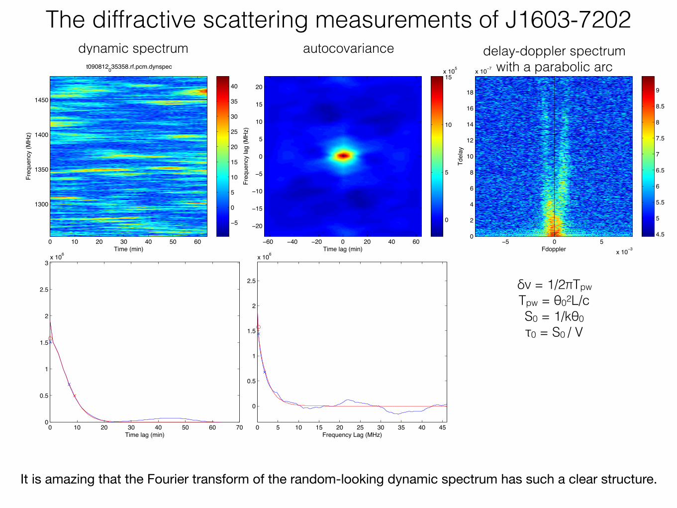
dynamic spectrum autocovariance delay-doppler spectrum with a parabolic arc

The diffractive scattering measurements of J1603-7202

δν = 1/2πTpw Tpw = θ02L/c S0 = 1/kθ0 τ0 = S0 / V

It is amazing that the Fourier transform of the random-looking dynamic spectrum has such a clear structure.

-10123

10-3

102

103

100

101

53500 54000 54500 55000 55500 56000 56500 57000

J1603-7202 ESE

This ESE is clearly extended and the obvious portion may simply be the leading edge.

The apparently random variation in time scale is larger than that in bandwidth.It is not completely random because it depends on the velocity.

no arcs no arcsarcs arcs

-3 -2 -1 0 1 2 3���� ����� �� �

0

50

100

150

200

250

300

350

400

���

���

��

��

���

����

���

���

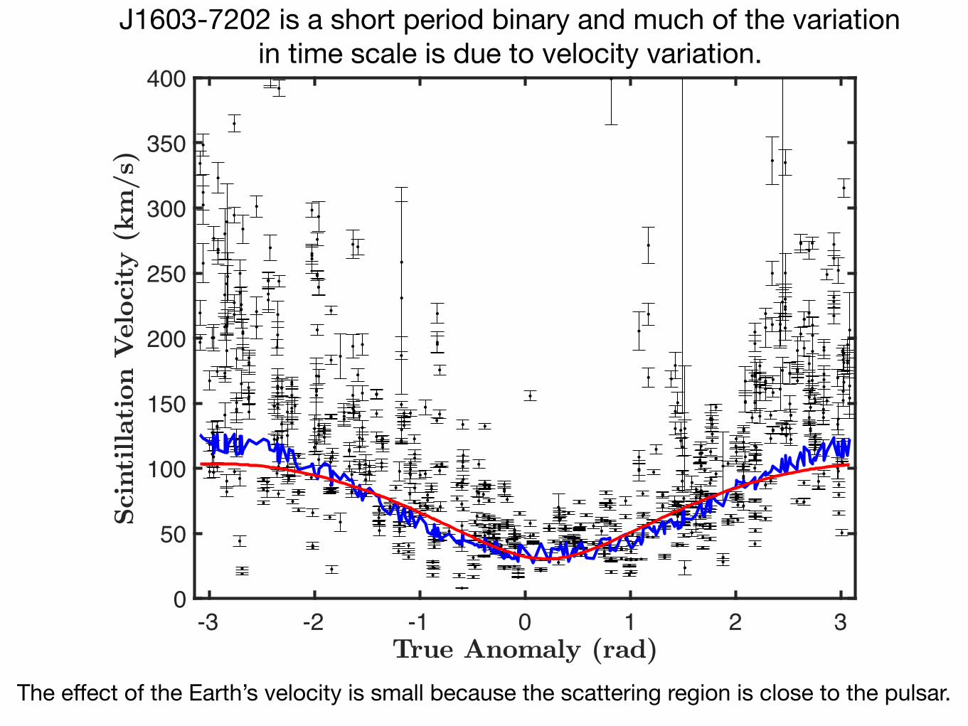
J1603-7202 is a short period binary and much of the variation in time scale is due to velocity variation.

The effect of the Earth’s velocity is small because the scattering region is close to the pulsar.

Several other PPTA pulsars also show enhanced scattering with a “hole”.

−1000 0 1000 2000−6

−4

−2

0

2

4x 10−4

MJD

DM

J0437−4715

−1000 0 1000 2000−1

−0.5

0

0.5

1x 10−3

MJD

DM

J0613−0200

−1000 0 1000 2000−2

−1

0

1

2x 10−3

MJD

DM

J0711−6830

−1000 0 1000 2000−1.5

−1

−0.5

0

0.5

1x 10−3

MJD

DM

J1022+1001

−1000 0 1000 2000−4

−2

0

2x 10−3

MJD

DM

J1024−0719

−1000 0 1000 2000−0.02

−0.01

0

0.01

0.02

MJD

DM

J1045−4509

−1000 0 1000 2000−4

−2

0

2

4x 10−3

MJD

DM

J1600−3053

−1000 0 1000 2000−4

−2

0

2

4x 10−3

MJD

DM

J1603−7202

−1000 0 1000 2000−10

−5

0

5x 10−3

MJD

DM

J1643−1224

−1000 0 1000 2000−1

−0.5

0

0.5

1x 10−3

MJD

DM

J1713+0747

−1000 0 1000 2000−4

−2

0

2

4x 10−3

MJD

DM

J1730−2304

−1000 0 1000 2000−0.015

−0.01

−0.005

0

0.005

0.01

MJD

DM

J1732−5049

−1000 0 1000 2000−1

−0.5

0

0.5

1

1.5x 10−3

MJD

DM

J1744−1144

−1000 0 1000 2000−0.015

−0.01

−0.005

0

0.005

0.01

MJD

DM

J1824−2452

−1000 0 1000 2000−3

−2

−1

0

1

2x 10−3

MJD

DM

J1857+0943

−1000 0 1000 2000−1

−0.5

0

0.5

1

1.5x 10−3

MJD

DM

J1909−3744

−1000 0 1000 2000−2

−1

0

1

2x 10−3

MJD

DM

J1939+2134

−1000 0 1000 2000−2

−1

0

1

2x 10−3

MJD

DM

J2124−3358

−1000 0 1000 2000−1

−0.5

0

0.5

1

1.5x 10−3

MJD

DM

J2129−5718

−1000 0 1000 2000−2

−1

0

1x 10−3

MJD

DM

J2145−0750

200cm-3 x 2AU

−1500 −1000 −500 0 500 1000 1500

−10

−5

0

5

x 10−4

DM

(t)

J0613−0200 1500MHz

−1500 −1000 −500 0 500 1000 1500

0

1

2

3

4

Flux

(mjy

)

−1500 −1000 −500 0 500 1000 15000

10

20

30

40

T DIF

F (min

)

−1500 −1000 −500 0 500 1000 15000

1

2

3

4

5

δν (M

Hz)

MJD − 55000

A “Hole” in PSR J0613-0200

This hole is obvious in scattering strength but less so in DM(t).

nature of the ISM (e.g., Cordes et al. 1986; Rickett &Lyne 1990). It has been shown that DM variations of somepulsars are consistent with those expected from an ISMcharacterized by a Kolmogorov turbulence spectrum (Cordeset al. 1990; Rickett 1990; Kaspi et al. 1994; You et al. 2007;Keith et al. 2013; Fonseca et al. 2014). One can calculate thestructure function of the varying DM:

DK

ft t

2DM DM , 3

22( ) ⟨[ ( ) ( )] ( )

⎛⎝⎜

⎞⎠⎟t

pt= + - ñj

where τ is a given time delay, K 4.148 103= ´MHz2 pc−1 cm3 s, and f is the observing frequency in MHz.

We expect, under the simplest assumptions, this function tofollow a Kolmogorov power law D 0

2( ) ( )t t t=jb- , where

11 3b = and 0t is a characteristic timescale related to theinner scale of the turbulence. The pulsars with DM variationsthat fit this theory generally have large DM variations ontimescale of years. However, PSR J1713+0747 does not showsignificant long-term DM variation (Figure 3). Conversely, itwent through a steep drop and recovery around 2008. If suchrapid DM changes are the result of variations in the ISM alongthe light of sight, such ISM variations do not fit the generalcharacteristics of a Kolmogorov medium.

3.3. Pulsar Spin Irregularity

The term “timing noise” in pulsar timing generally refers tothe non-white noise left in the timing residuals. An importantcontribution to timing noise is expected to come from thepulsarʼs spin irregularity, i.e., its long-term deviation from asimple linear slow down. Spin irregularity is often significant inyounger pulsars, and may be modeled with high-orderfrequency polynomials (such as n , where ν is the pulsarʼs spinfrequency). Potential causes of irregular spin behavior includeunresolved micro-glitches, internal superfluid turbulence,magnetosphere variations, or external torques caused by mattersurrounding the pulsar (Hobbs et al. 2010; Yu et al. 2013;Melatos & Link 2014). These mechanisms could lead toaccumulative random perturbations in the pulsarʼs pulse phase,spin rate, or spin-down rate. Shannon & Cordes (2010) pointedout that one could model these types of timing noise usingrandom walks. Random walks in phase (RW0) would growover time (T) proportionally to T1 2, random walks in ν growproportionally to T3 2, random walks in n grow proportionallyto T 5 2. Such spin noise would likely have a steep power

Table 5The Timing Results from Splaver et al. (2005) and from a Re-analysis of the Splaver et al. (2005) Data Set Using New Red Noise Analysis Technique

Parameter Splaver et al. (2005) Red Noise Modela

R.A., α (J2000) 17:13:49.5305335(6) 17:13:49.5305321(6)decl., δ (J2000) 7:47:37.52636(2) 7:47:37.52626(2)Spin frequecy ν (s−1) 218.8118439157321(3) 218.811843915731(1)Spin down rate n (s−2) 4.0835 2 10 16( )- ´ - 4.0836 1 10 16( )- ´ -

Proper motion in α, cos˙m a d=a (mas yr−1) 4.917(4) 4.917(4)Proper motion in δ, ˙m d=d (mas yr−1) −3.93(1) −3.93(1)Parallax, ϖ (mas) 0.89(8) 0.84(4)Dispersion measure (pc cm−3) 15.9960 15.9940Orbital period, Pb (day) 67.8251298718(5)b 67.825129921(4)Change rate of Pb, Pb˙ (10−12 s s−1) 0.0(6) −0.2(7)Eccentricity, e 0.000074940(1)b 0.000074940(1)Time of periastron passage, T0 (MJD) 51997.5784(2)b 51997.5790(6)Angle of periastron, ω (deg) 176.192(1)b 176.195(3)Projected semimajor axis, x (lt-s) 32.34242099(2)b 32.3424218(3)Cosine of inclination, icos 0.31(3) 0.32(2)Companion mass, Mc (M:) 0.28(3) 0.30(3)Position angle of ascending node, Ω (deg) 87(6) 89(4)Solar system ephemeris DE405 DE405Reference epoch for α, δ, and ν (MJD) 52000 52000Pulsar mass, MPSR (M:) 1.3(2) 1.4(2)Red noise amplitude (μs year1 2) L 0.004Red noise spectral index L 5.14

Notes.a We used TEMPO2ʼs T2 binary model, which models the Keplerian (Pb, x, e, T0, and ω) and post-Keplerian orbital elements ( icos , Ω, and m2 ) simultaneously.b Splaver et al. (2005) uses TEMPOʼs DD model and reports the uncertainties of the Keplerian parameters with the post-Keplerian ones fixed to their bestfit values.

Figure 3. Plot shows 16-year DM variation of PSR J1713+0747. The dottedline shows the Solar elongation of the pulsar. The subplot shows the structurefunction (error bars) and its a power-law fit (solid line). The best-fit power-lawindex is 0.49(5), different from the value of 5 3 expected from a “pure”Kolmogorov medium.

9

The Astrophysical Journal, 809:41 (15pp), 2015 August 10 Zhu et al.

Hole in the J1713+0747 NanoGrav observations, Zhu, Weiwei et al. 2015.

This cannot be due to a pc scale structure, it must be a thin screen, of AU thickness. It does not show a clear change in scattering.

106 108 1010 1012 1014 1016 101810−5

100

105

1010

1015

1020

Scale (m)

Phas

e St

ruct

ure

Func

tion

(rad2 )Dφ(S)

LOS

ESE

Holes and ESEs imply very thin scattering regions because they have transverse size ~ AU, they cannot have line of sight size more than 10s of AU.

How does such a small change in DM ~ 1:104, caused by an AU size structure increase the scattering on a line of sight 100s of pc long, by factor of 10?

The ESE is more effective at scattering than the entire LOS for two reasons: (1) The LOS is averaged over 1600 outer scales and the ESE over only a few;(2) The ESE saturates at its Sout = a few AU, but the LOS at Sout = a few pc.

Summary of DM Variations

When pulsars were discovered, one of the first questions answered was “are the electrons causing DM the same as those causing the scattering?” We now know that the answer is “SOMETIMES”.

Sometimes the scattering is dominated by a tiny, extremely turbulent region that contributes almost nothing to DM.

This is an extreme form of intermittency which is common in other large Reynold’s number fluids, such as the atmosphere and the ocean.

We are not sure what causes this, but a likely possibility in the IISM is turbulence caused by shear instabilities when two IISM clouds interact. Such instabilities start at small scales and grow in both amplitude and spatial scales.

To interpret the secondary spectrum we consider a scattered image consisting of a smooth anisotropic core and some discrete bright points

κY

=kθY

κX

=kθX

V

κX

=kθX

κY

=kθY

FDOP

TDEL

FDOP

TDEL

Image

correspondingsecondary

spectra

What are these parabolic arcs and why are they interesting?

Diffe

ren

tial D

op

ple

r freq

ue

ncy fD

(mH

z)

Differential Delay τ (ms)

−60

−40

−20

020

40

60

0

0.2

0.4

0.6

0.8 1

1.2

1.4

1.6

1.8 2

7.5

8 8.5

9 9.5

10

10.5

11

11.5

12

Diffe

rentia

l Dopple

r frequency fD

(mH

z)

τ

−6

0−

40

−2

00

20

40

60

0

0.2

0.4

0.6

0.8 1

1.2

1.4

1.6

1.8 2

−1

50

−1

00

−5

0

0 50

10

0

15

0

Fig.

1.—T

he

amplitu

de

(left)an

dphase

(right)

ofth

esecon

adary

crosssp

ectrum

C,defi

ned

inTab

le1,

forth

e8

MH

zw

ide

314.5M

Hz

sub-b

and

onth

eA

O-G

BT

baselin

e.A

mplitu

de

scaleis

log10

and

phase

isin

degrees

For

disp

laypurp

oseson

ly,both

diagram

shave

been

smooth

edover

5pix

elsin

delay

tored

uce

the

noise,

givin

gplotted

resolution

of0.44

mH

zin

Dop

pler

frequen

cyan

d3.1

µs

indelay.

The

black

line

isa

parab

olaw

ithcu

rvature

0.56s3

onboth

pan

els.T

here

arebrigh

tarclets

inam

plitu

de

that

extend

along

the

ridge

ofth

ism

ainparab

olato

delay

s>

1m

s.T

he

phase

appears

much

smooth

er,as

discu

ssedin

§3.1.

tance

Dp

fromE

arth,

whose

radiation

isscat-

teredby

anin

hom

ogeneou

sregion

ofion

izedin

-terstellar

med

ium

ata

distan

ceD

sfrom

Earth

.In

this

thin

-screenap

prox

imation

the

phasor

due

torad

iationscattered

ata

poin

tx

j=

Ds θ

jin

the

screensuffers

aphase

delay

φj

due

toth

escatterin

gplasm

aan

dis

receivedw

itha

totalphase

delay

Φj (r)

=φ

j+

k(x

j −βr)

2/2βD

sw

here

β=

1−

Ds /D

pan

dr

isth

etran

sverseposition

ofth

ereceiv

ing

anten

na.

The

receivedelectric

field

isth

esu

mm

ationof

all such

scatteredcom

po-

nen

ts,eith

erex

pressed

by

the

Fresn

eldiff

ractionin

tegral(see

Cord

eset

al.2006)

orap

prox

imated

by

asu

mm

ationover

allstation

aryphase

poin

ts(see

Walker

etal.

2004),in

strong

scattering.

Here

we

use

the

stationary

phase

approx

ima-

tionto

obtain

the

correlationof

the

field

sbetw

eenan

tennas

atlo

cations−

b/2

and

b/2.

This

defi

nes

the

visib

ilityw

hose

Fou

riertran

sformin

time

and

frequen

cycan

be

written

as:

V(τ, f

D,b

)=

!j,k

exp[i(Φ

j (−b/2)−

Φk (b

/2))]

×µ

j µk δ(f

D−

fD

,jk )δ(τ−

τjk ).

(2)

where:

fD

,jk=

1λ(θ

j −θ

k ) ·V

eff,

(3a)

τjk

=D

s

2cβ

(θ2j−

θ2k )

+

"

φj

2πν−

φk

2πν

#

.(3b)

The

δfu

nction

sin

equation

(2)determ

ine

how

eachparticu

larpoin

ton

the

secondary

spectru

mis

relatedto

apair

ofpoin

tsin

the

screen.

With

finite

ban

dw

idth

and

observ

ing

time

the

δfu

nc-

tionssh

ould

be

replaced

by

finite

narrow

sinc

func-

tions.

The

equation

sum

sover

allpossib

lepairs

ofstation

aryphase

poin

tsin

the

screen,w

ithµ

j , µk

asth

em

agnifi

cations

determ

ined

by

phase

cur-

vature

ofeach

poin

t(see

Walker

etal.

2004).In

the

full

Fresn

elform

ulation

,th

esu

mm

ationbe-

comes

adou

ble

two-d

imen

sional

integration

over

5

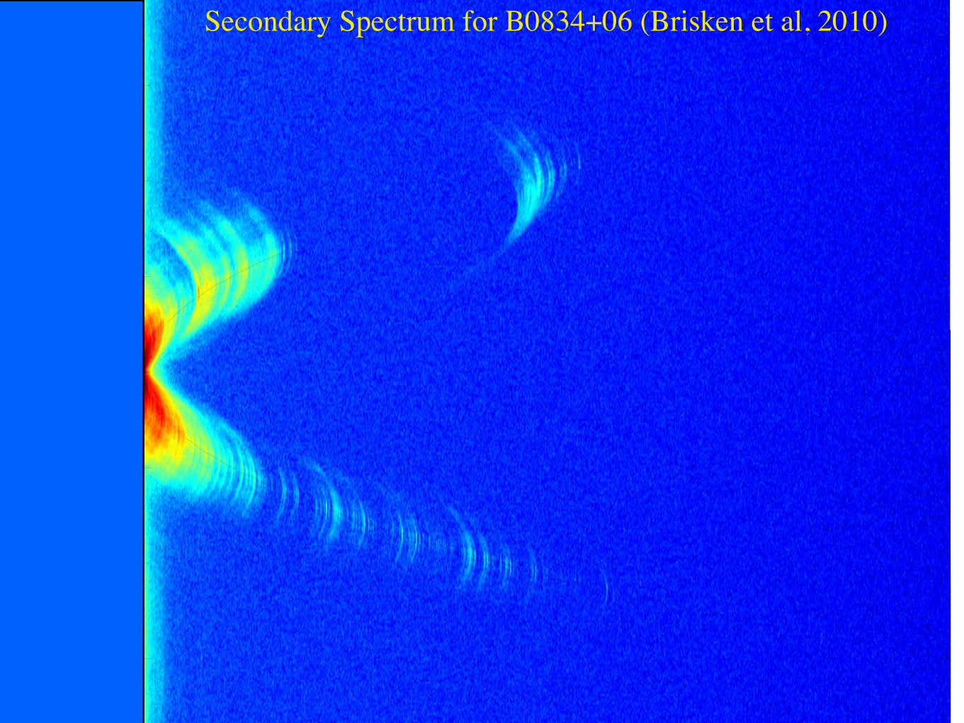
Secondary Spectrum for B0834+06 (Brisken et al, 2010)

core

astrometry

inversion

Reconstructed Image

3 AU

137

is tilted in the same direction as chapter 2. The brightness integrated over perpen-

dicular direction matches the 1-D Bk(✓k) estimated in chapter 2. The brightness

integrated over parallel direction which gives the estimate of B?(✓?) shows more

homogenous distribution.

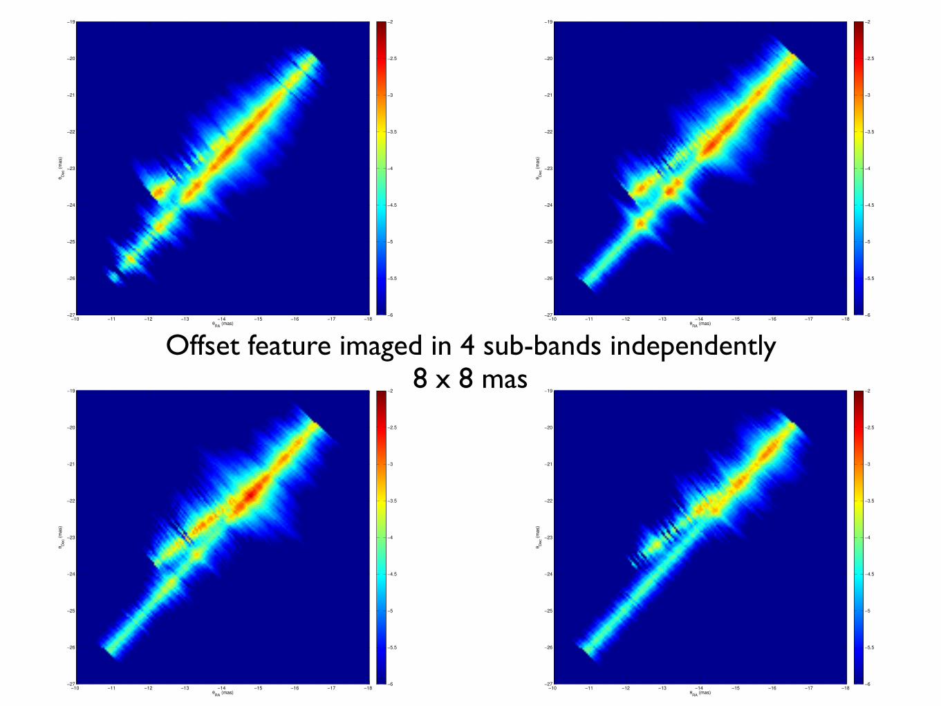
Figure 6.1: Estimated 1-D brightness distribution including both primary ando↵set feature, with dynamic range between -4 to 0. The o↵set feature in the redsquare is expanded in Figure 6.2 below.

In chapter 4, we analyzed a di↵erent data set, but of the same pulsar. We

developed an imaging technique based on the electric field representation, which

has a two-fold ambiguity. As in Figure 4.5 it shows the same parallel direction as

in chapter 2 and 3. However, due to the lack of phase information, the position

Is it reasonable to characterize this thing as a stochastic process?

138

ambiguity can’t be solved, especially in the core image. We noticed four features

in Figure 4.5, one of which (RA=-5mas, Dec=8mas) is far o↵ the main parallel

axis of the primary feature which was not seen in the results of those two previous

chapters.

θRA

(mas)

θD

ec (

mas)

−18−17−16−15−14−13−12−11−10−27

−26

−25

−24

−23

−22

−21

−20

−19

−6

−5.5

−5

−4.5

−4

−3.5

−3

−2.5

−2

θRA

(mas)

θD

ec (

mas)

−18−17−16−15−14−13−12−11−10−27

−26

−25

−24

−23

−22

−21

−20

−19

−6

−5.5

−5

−4.5

−4

−3.5

−3

−2.5

−2

θRA

(mas)

θD

ec (

mas)

−18−17−16−15−14−13−12−11−10−27

−26

−25

−24

−23

−22

−21

−20

−19

−6

−5.5

−5

−4.5

−4

−3.5

−3

−2.5

−2

θRA

(mas)

θD

ec (

mas)

−18−17−16−15−14−13−12−11−10−27

−26

−25

−24

−23

−22

−21

−20

−19

−6

−5.5

−5

−4.5

−4

−3.5

−3

−2.5

−2

Figure 6.2: The same as Figure 6.1, zoom in o↵set feature region, with dynamicrange between -6 to 2, four di↵erent channels. upper-left: Channel 1, upper-right:Channel 2, lower-left: Channel 3, lower-right: Channel 4

In chapter 5, curvi-line linear feature model is used on primary feature, and

two straight-line linear model is used on o↵set feature. Figure 5.15 and Figure 5.34

show the brightness distribution and ✓? fluctuation for primary feature and o↵set

feature. Figure 5.18 and Figure 5.31 show the geometry of primary feature and

o↵set feature. It’s hard to combine them to give a good picture of their bright-

Offset feature imaged in 4 sub-bands independently8 x 8 mas

Some Interesting Observations of PSR B1737+13 by Dan Stinebring

This behavior continued for 99 days, and on day 106 it stopped. No more arcs were visible. This suggests the passage of an extended thin ESE region such as seen in J0613-0200, J1603-7202, & J1713+0747.

Summary

Things that look like ESEs are more common in both DM(t) observations and diffractive scattering observations, than they appear to be in observations of refractive AGN flux variations.

Similar “events” with AU spatial scales are frequently seen in delay-Doppler spectra, particularly of nearby pulsars.

It seems likely that the “events” seen in “secondary spectra,” such as B0834+06 and B1737+13, are ESEs. The classic ESE seen in AGN observations, may simply be, one which has exactly the right “focal length”, but is a subset of a much larger class of irregular objects.

Measurements of the curvature of parabolic arcs can be much more precise than time scale and bandwidth, particularly for pulsars in relatively weak scattering. Daniel Reardon has recently located the scattering regions in PSR J0437-4715 within a light year and measured the ISM velocity within 1 km/s.

Back to gravitational waves. We must understand our noise sources if we are to remove them completely. We have to understand the IISM!