Grapevine Remote sensing Analysis of Phylloxera Early ... · Remote sensing Analysis of Phylloxera ... the California State University, and Robert Mondavi Winery examined the application

NASA Technical Memorandum 112218

1

Grapevine Remote sensing Analysis of Phylloxera Early Stress (GRAPES): Remote Sensing Analysis Summary∗

Brad Lobitz1, Lee Johnson2, Chris Hlavka3, Roy Armstrong 4, and Cindy Bell5

1 Johnson Controls World Services, Inc., Ames Operation (currently California StateUniversity, Monterey Bay)

2 Johnson Controls World Services, Inc., Ames Operation (currently California StateUniversity, Monterey Bay)

3 NASA Ames Research Center, Earth Science Division4 Johnson Controls World Services, Inc., Ames (currently Univ. Puerto Rico)5 Johnson Controls World Services, Inc., Ames Operation (currently California State

University, Monterey Bay)

Abstract

This document describes image processing analysis applied to high spatial resolution

airborne imagery acquired in California's Napa Valley in 1993 and 1994 as part of the Grapevine

Remote sensing Analysis of Phylloxera Early Stress (GRAPES) project. Investigators from

NASA, the University of California, the California State University, and Robert Mondavi

Winery examined the application of airborne digital imaging technology to vineyard management,

with emphasis on detecting the phylloxera infestation in California vineyards. Phylloxera

infestation is a significant problem because the root louse causes vine stress that leads to

grapevine death in three to five years. Eventually the infested areas must be replanted with

resistant rootstock. Visual symptoms of phylloxera infestation include leaf chlorosis, vine size

reduction, and collapse of fruit tissue during the growing season. Increased leaf temperatures have

also been hypothesized for affected vines. Early detection of infestation and changing cultural

∗ full citation: Lobitz, B., L. Johnson, R. Armstrong, C. Hlavka and C. Bell. 1997.Grapevine Remote Sensing Analysis of Phylloxera Early Stress (GRAPES):Remote Sensing Analysis Summary. NASA Technical Memorandum No. 112218,December 1997.


2

practices to compensate for vine damage can minimize crop financial losses from damage and

replanting. Vineyard managers need improved information to decide where and when to replant

fields or sections of fields.

Multi-year airborne images of a vineyard were spatially co-registered so annual relative

changes in leaf area due to phylloxera infestation could be located. Image processing analysis was

applied to data from the Compact Airborne Spectrographic Imager (CASI, imagery acquired in

1993) and the Electro-Optic Camera (EO Camera, imagery acquired in 1994). Changes were

determined by using information obtained from computing Normalized Difference Vegetation

Index (NDVI) images. As the canopy leaf area of infested regions decreased, these regions became

increasingly non-uniform. Infestation spread was also projected in advance using proximity

analysis, a geographic information system (GIS) technique. Two other methods of monitoring

vineyards through imagery were also investigated: optical sensing of the Red Edge Inflection

Point (REIP), and thermal sensing. These did not convey the stress patterns as well as the NDVI

imagery and require specialized sensor configurations. NDVI-derived products are recommended

for monitoring phylloxera infestations.

Introduction

Phylloxera (Daktulosphaira vitifoliae Fitch) affects a number of the grape growing

counties in California and is currently a severe problem in Napa and Sonoma Counties. The

parasitic action of this root louse causes leaf chlorosis, decreases shoot and leaf growth and fruit

yield, and leads to vine death three to five years from onset. Once established, the infestation

spreads quickly through a vineyard. The grapevines' deep rooting pattern makes pesticides

ineffective and there is no known biological control (Granett et al., 1987 and 1991).

Changing cultural practices, such as adjusting pruning severity or changing the amount of


3

irrigation, are sometimes used to prolong fruit production, but there is little the grape grower can

do to combat phylloxera, except replant on phylloxera-resistant rootstock. As the infestation

spreads, the grape yield decreases each year, until the yield is too low justify the maintenance

costs and the vines are plowed up. Replanting is expensive, and the field will also be out of

production for a number of years before the newly planted vines bear fruit.

The Grapevine Remote sensing Analysis of Phylloxera Early Stress (GRAPES) project

was a collaboration between NASA Ames Research Center, the University of California Davis,

the University of California Cooperative Extension, California State University Chico, and

Robert Mondavi Winery (Oakville, CA). The project was developed to demonstrate the use of

remotely sensed data for vineyard management, with emphasis on monitoring phylloxera

infestation, e.g., using remotely sensed data to help decide when to replant a phylloxera infested

field.

Some vineyard managers have used aerial photography to study phylloxera spread

(Wildman, 1983). The GRAPES project incorporated airborne digital imaging systems with

subsequent image processing and analysis to enhance information content with respect to canopy

size (Johnson et al., 1996). This report summarizes methodology used to generate annual imagery

for vineyard managers to monitor the spread of phylloxera in a Mondavi vineyard. This

methodology could be applied to digitally acquired imagery and to film-based traditional aerial

photography that has been scanned into digital form. Satellite images acquired by the Landsat

Thematic Mapper (TM) and Satellite Pour l'Observation de la Terre (SPOT) were also

purchased, but were used for valley wide analysis and not at the vineyard or block scale. (A

block is the smallest management unit within a vineyard.) This document also describes the image

processing analysis applied to high spatial resolution airborne imagery acquired in California's

Napa Valley in 1993 and 1994. Results of the analysis indicate the procedures used offer tangible


4

benefits to growers.

Study Site and Ground Data

Airborne digital data were acquired over the study site, ToKalon Ranch (a vineyard

owned and managed by the Robert Mondavi Winery), in 1993 and most of Napa Valley,

including ToKalon and two other Mondavi vineyards: Carneros and Oak Knoll, in 1994.

ToKalon ranch lies on the West edge of the valley floor and is surrounded on the other three sides

by other vineyards. The ToKalon soils are mainly Bale loam and clay loam with 0-2% slope,

with some Bale clay loam with 2-5% slope and some Coombs gravelly loam with 0-2% slope.

The southern portion of the ranch is Clear Lake clay (2-5% slope). Images from 1993 and 1994

covering all of ToKalon Ranch were processed, but this report focuses on one five-hectare block

(denoted as block I in the following discussion) within ToKalon. Block I consisted of cabernet

sauvignon grapevines on AXR-1 rootstock with four-meter row spacing planted primarily in

Clear Lake clay soil. The analysis of this block was used to illustrate the type of information that

can be generated for an entire vineyard.

Nine plots within block I were used for collecting field data (pruning weights, phylloxera

counts, and leaf samples). These plots were chosen based on 1992 aerial color infrared

photography and a pre-growing season phylloxera study. Interpretation of the color infrared

photos provided locations of infested areas. Infestation levels were then confirmed by root

digging in the field. The nine plots consisted of three plots each of uninfested, mildly infested,

and severely infested vines. Each plot contained forty vines. At the end of each growing season

(January), Mondavi pruned the vines and weighed vegetative material. Infrared temperatures

were also collected in the field, using a hand held infrared thermometer, from five representative

plots, soil, and roads in 1994. These data were used to support airborne thermal infrared data


5

collection.

Aircraft Data

Aerial photography (acquired by Ames Research Center's C-130 and ER2 aircraft) and

digital imagery from a variety of airborne sensors were used during the GRAPES project. Several

airborne sensors with different specifications and spectral characteristics were used to investigate

block monitoring capabilities and to test the utility of the digital image processing methods.

The airborne sensors used included: Airborne Data Acquisition and Registration (ADAR),

Airborne Infrared Disaster Assessment System (AIRDAS), Compact Airborne Spectrographic

Imager (CASI), Digital Multi-Spectral Video (DMSV), Electro-Optic Camera (EO Camera),

NS001 Thematic Mapper Simulator (TMS), and Real Time Digital Airborne Camera System

(RDACS). Each of these sensors can be used to acquire image data at different spatial, spectral,

and radiometric resolutions. Spatial resolution, or ground resolution, is the size of the smallest

area element that can be detected for the image. Spatial resolution, referred to as pixel size,

depends on the sensor platform (aircraft) collection altitude. For example, the CASI sensor can be

used to acquire image data at spatial resolutions between 0.6 m and 10 m. At 1200 m altitude, the

CASI system yields a pixel size of 1.6 m (rounded to 2 m in this report) and at 450 m, 0.6 m.

The total area imaged, therefore, decreases with decreasing aircraft altitude. Below some limiting

height the sensor systems cannot acquire and store data fast enough to provide continuous

ground coverage. The AIRDAS (Ames Research Center) sensor, which was designed for fire

monitoring, has two thermal infrared channels (Ambrosia et al., 1994). The AIRDAS low

temperature, thermal channel (9250 nm center wavelength) was the most interesting for the

GRAPES project, because it was used to determine surface (brightness) temperatures. The CASI

can be used to collect data in spatial mode and spectral mode. In the CASI's spatial mode the


6

sensor functions as a push-broom imager with up to 15 bands and in spectral mode the sensor

operates like a group of spectrometers (1.8 nm spectral resolution) sweeping the flight path

(Borstad Assoc., 1991). Only the spatial mode with four or eight channels and a resampled

spatial resolution of about 2.0 m were used for the project. The four channel configuration was

used to provide false color infrared imagery and the eight channel configuration provided data

along the red edge of the vegetation reflectance curve, Figure 1. The DMSV had four similar

channels (Lyon, 1994). The EO Camera, flown at an altitude of 20 km aboard the NASA ER-2,

has a nominal spatial resolution of five meters and was flown with five channels. The NS001

TMS has eight channels, was flown aboard the NASA C-130 with a spatial resolution of three to

five meters. Seven of these channels correspond to the TM instrument channels. The RDACS

has three cameras with narrow band filters (about ten nanometers). While the imagery acquired

from all these sensors was examined, most of the data analysis was performed on data from the

primary project sensors (CASI and EO Camera). Data from the other sensors were provided by

their representatives for evaluation. Only the CASI and EO Camera processing will be discussed

in the following sections. The central wavelengths of each spectral channel, the spatial resolution,

and the sensor provider for these sensors are summarized in Table 1. For more detailed sensor

specifications, see the Appendix.

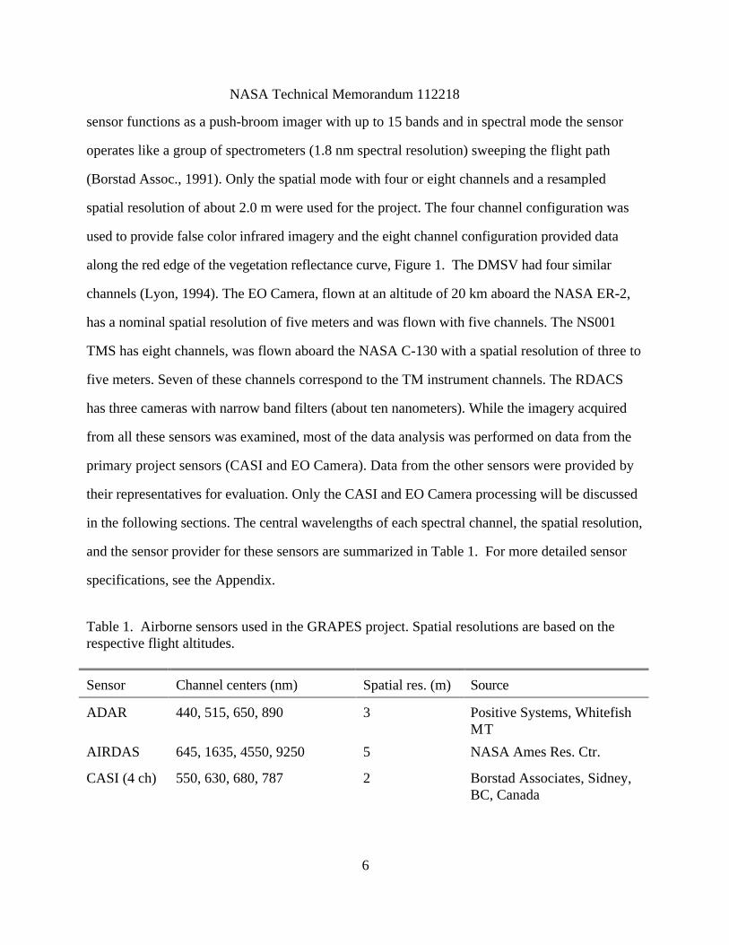
Table 1. Airborne sensors used in the GRAPES project. Spatial resolutions are based on therespective flight altitudes.

Sensor Channel centers (nm) Spatial res. (m) Source

ADAR 440, 515, 650, 890 3 Positive Systems, WhitefishMT

AIRDAS 645, 1635, 4550, 9250 5 NASA Ames Res. Ctr.

CASI (4 ch) 550, 630, 680, 787 2 Borstad Associates, Sidney,BC, Canada


7

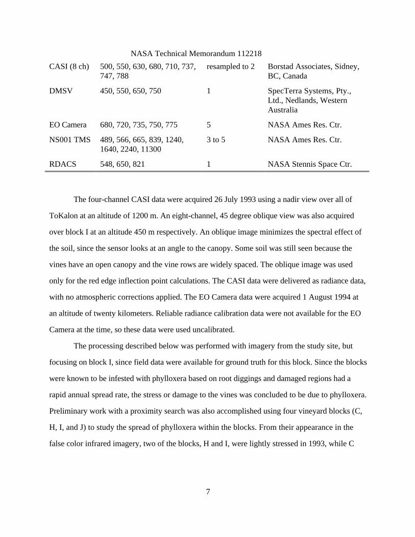
CASI (8 ch) 500, 550, 630, 680, 710, 737,747, 788

resampled to 2 Borstad Associates, Sidney,BC, Canada

DMSV 450, 550, 650, 750 1 SpecTerra Systems, Pty.,Ltd., Nedlands, WesternAustralia

EO Camera 680, 720, 735, 750, 775 5 NASA Ames Res. Ctr.

NS001 TMS 489, 566, 665, 839, 1240,1640, 2240, 11300

3 to 5 NASA Ames Res. Ctr.

RDACS 548, 650, 821 1 NASA Stennis Space Ctr.

The four-channel CASI data were acquired 26 July 1993 using a nadir view over all of

ToKalon at an altitude of 1200 m. An eight-channel, 45 degree oblique view was also acquired

over block I at an altitude 450 m respectively. An oblique image minimizes the spectral effect of

the soil, since the sensor looks at an angle to the canopy. Some soil was still seen because the

vines have an open canopy and the vine rows are widely spaced. The oblique image was used

only for the red edge inflection point calculations. The CASI data were delivered as radiance data,

with no atmospheric corrections applied. The EO Camera data were acquired 1 August 1994 at

an altitude of twenty kilometers. Reliable radiance calibration data were not available for the EO

Camera at the time, so these data were used uncalibrated.

The processing described below was performed with imagery from the study site, but

focusing on block I, since field data were available for ground truth for this block. Since the blocks

were known to be infested with phylloxera based on root diggings and damaged regions had a

rapid annual spread rate, the stress or damage to the vines was concluded to be due to phylloxera.

Preliminary work with a proximity search was also accomplished using four vineyard blocks (C,

H, I, and J) to study the spread of phylloxera within the blocks. From their appearance in the

false color infrared imagery, two of the blocks, H and I, were lightly stressed in 1993, while C


8

and J were moderately stressed in 1993. In 1994, blocks H and I were moderately stressed and

block C was severely stressed and block J was moderately stressed.

A 1993 C-130 1:6 000 scale and a 1994 ER2 1:32 000 scale photograph were also

available for the ToKalon Ranch region. The photographs were scanned to generate multispectral

images, analogous to the NIR, red, and green channels of an airborne scanner. The effective pixel

size for these images after registration was one meter.

Processing and Results

There were several factor affecting the image analysis procedures: (1) the image data had

to be in the same map projection as, and spatially co-registered with, the other data layers used in

the GRAPES project (e.g., soils, road network, hydrology); (2) the imagery was to be compared

from year to year; and (3) the data analysis procedures needed to be practical and applicable for

procedural repeatability and ease of use. The third factor required choosing a procedure providing

results easily comparable with the field data.

The second constraint was the most difficult to achieve. The data processing had to

reconcile differences in sensor characteristics and provide results that were not affected by

differences in viewing conditions. Several normalization schemes were tested to reconcile the data

sets. The scheme finally selected was chosen based on ease of implementation and validity of the

results. The simplest procedure was to match the spatial resolutions of the data, then classify the

imagery based on the Normalized Difference Vegetation Index (NDVI) values. This simple

method provided sufficient results without complicated sensor calibration and atmospheric

correction models applied to the imagery.

Image Registration


9

The four-channel CASI imagery acquired in 1993 was used as the base date, while

subsequent airborne digital images were geo-registered to it. The ToKalon site data, consisting of

three adjacent passes, were mosaicked together into one image. The mosaicked image was

registered to a Universal Transverse Mercator (UTM) zone ten projection, with two-meter

spatial resolution. This image registration was accomplished using global positioning system

(GPS) data points collected in the field. These points were then located in the image and used as

ground control points (GCP's). Finally, the image was warped so the GCP's were in the correct

positions relative to the UTM coordinate system. Later images of the same area, such as the EO

Camera imagery, were registered to this image. A standard image to image transformation

procedure was used. In this case the GCP's were pixel locations in the CASI image and the

equivalent pixel locations in the unregistered image.

Equalization of Spatial Resolution

The EO Camera imagery, acquired in 1994, was registered to the 1993 CASI imagery. The

1994 EO Camera data had a nominal spatial resolution of five meters, while the CASI imagery

had a spatial resolution of two meters. The resolution difference was compounded by the EO

Camera lens could not be focused across all wavelength channels simultaneously, and

consequently the channels, particularly the red channel, were slightly out of focus. The 1994

image was registered to the 1993 image, while adjusting for the pixel size (sampling interval)

difference by resampling. Low pass (averaging) spatial filters of various sizes were used to

degrade the CASI and EO Camera near infrared (NIR) to the EO Camera red spectral band spatial

resolution. The best visual match was obtained with a 5x5 window applied to the EO Camera

NIR band and a 7x7 window applied to both of the CASI channels. This procedure normalized

the EO Camera focusing problems, Figure 2.


10

Normalized Difference Vegetation Index Analysis

The NDVI was next applied to the imagery. The NDVI is defined as

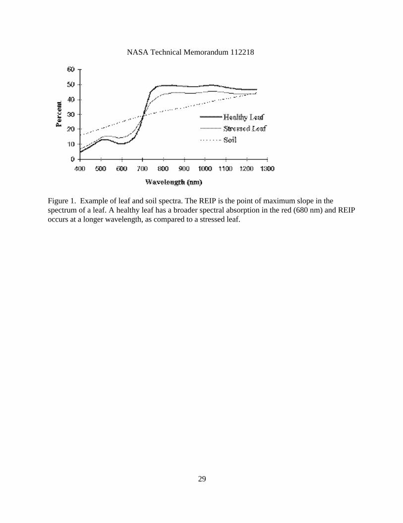
The NDVI highlights differences in vegetation canopy reflectance. Healthy vegetation has strong

absorbance characteristics in the red portion of the electromagnetic spectrum (EMS), while also

reflecting strongly in the NIR portion of the EMS. These properties are due to the interaction of

light with the chlorophyll in the plant tissue, Figure 1. Subtle changes in vegetation vigor or leaf

chlorophyll composition result in subtle alterations in absorbance and reflectance characteristics.

These characteristics are then highlighted in the NDVI. The index is near zero for bare soil, but

can be close to 1.0 for a dense, healthy canopy. The NDVI was used because it lessens the

influence of solar illumination, angular influences, slope, and viewing geometry. It performs

consistently between sensors, for different flights, and within the images. NDVI is also correlated

to leaf area index (LAI), or canopy leaf amount, and biomass (Tucker 1979). The index

compensates for brightness differences and highlights the spectral differences between pixels.

Absolute NDVI's were not directly comparable because of year-to-year differences in non-

canopy variables and non-phylloxera related growth effects. Non-canopy variables include

calibration differences (the CASI data were calibrated to radiance versus the raw EO Camera

data), atmospheric conditions (weather conditions and aerosol concentration), and solar

illumination angle differences. Year to year plant growth differences could be also be a response

to other factors, including other plant stresses, changes in management practices, and increased

rainfall (i.e., more irrigation) in 1994. However, if the range of NDVI values within the images is

represented by classes, then relative values (classes) in the images from the same areas on

NDVI =NIR - redNIR+red

.


11

different dates can be compared. A small number of classes makes the images easier interpret.

Initially NDVI data were assigned hues ranging from brown (bare soil), through yellow (small or

stunted vines), to dark green (vigorous growth). This approach showed damage patterns within

the vineyard. Later, images were coded using a rainbow (color spectrum) color coding due to the

greater hue separation. This scheme was preferred by the Mondavi vineyard manager and

subsequently because the coding of choice for the images.

Subjective comparisons of NDVI images of block I from 1993 and 1994 were difficult, so

an unsupervised classification was used to categorize block I and, later, the entire vineyard. An

objective method of determining class breaks was needed, so Iterative Self-Organizing Data

Analysis (ISODATA, Duda and Hart, 1973), an unsupervised classification algorithm was used.

Utilized with only one input image band, the ISODATA routine determines the clusters within

the range of pixel values in the image using the number of clusters the user inputs. The

ISODATA classification process begins by dividing the range of values and using the midpoint of

each breakpoint as the starting means for the number of classes specified by the user. Each pixel

is then assigned to the cluster that has the closest mean value to the pixel value. Cluster means are

then recomputed based on the pixels assigned to the clusters, and the pixels are again assigned to

clusters based on the new means. Eventually the means settle down and the process terminates.

When run on block I, six classes were used in the classification. This kept the number of classes

down ease of interpretation, while still representing the image variation. For the entire vineyard,

this number was doubled to twelve classes, since there was much variation in NDVI values due to

differences in vine maturity, trellis type, and vine spacing as well as plant condition.

A number of vineyard blocks were pulled after the 1993 data acquisition, and,

subsequently, large areas of bare soil were evident in the 1994 imagery. These "soil" pixels would

be over-represented in the classes generated from the 1994 NDVI image. To equalize the


12

distribution, the NDVI images were visually compared with aerial photos and the false color

infrared imagery to select an NDVI threshold that masked out the nearly bare and bare soil pixels.

Any pixels below the threshold (the soil) became zero and were not considered in the

classification routine. The thresholded image contained only vegetated landscape elements and the

range of NDVI values was therefore reduced. The proportion of high NDVI pixels appeared

stable, since those pixels were primarily trees along the streams, roads, and hillside as well as the

vigorous grapevines.

The ISODATA classification was performed to the filtered CASI (1993) and EO Camera

(1994) images. A common area covering the ToKalon vineyard was used in these steps for both

years. Subsets of each of these classified images for block I are shown in Figure 3. The mean

class values for each of the plots within block I and their pruning weights are shown in Table 2.

A percentage summary of the classification for block I by class values is shown in Figure 4. In

the vineyard as a whole, there were NDVI class values below and above the block I class values.

A few NDVI classes predominated in 1993 (Figure 4). In 1994, the vineyard blocks had a large

number of bare soil pixels and a broad distribution of other class values, because phylloxera

damage lead to a decrease in block uniformity.

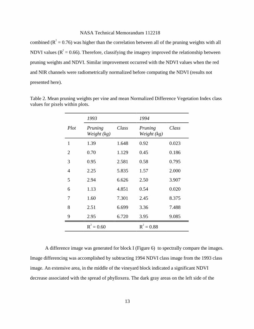
The 1994 histogram for block I (Figure 4) also showed increases in high class values,

which was consistent with the pruning weights given for plots 7 - 9 (Table 2). Infestation levels

were evident in the pruning weights and to a lesser extent in the NDVI class values. Table 2

indicates the mean class values for the pixels in infested plots 1 - 6 had decreased, while the mean

class values for the lightly or unaffected plots (7, 8, and 9) had increased. Class values were

plotted against pruning weight in Figure 5. Correlations between the pruning weights and either

NDVI or class values were similar, though greater in 1994 versus 1993: R2 was about 0.60 for

1993, 0.86 for 1994. The correlation between pruning weight and NDVI class for both years


13

combined (R2 = 0.76) was higher than the correlation between all of the pruning weights with all

NDVI values (R2 = 0.66). Therefore, classifying the imagery improved the relationship between

pruning weights and NDVI. Similar improvement occurred with the NDVI values when the red

and NIR channels were radiometrically normalized before computing the NDVI (results not

presented here).

Table 2. Mean pruning weights per vine and mean Normalized Difference Vegetation Index classvalues for pixels within plots.

1993 1994

Plot PruningWeight (kg)

Class PruningWeight (kg)

Class

1 1.39 1.648 0.92 0.023

2 0.70 1.129 0.45 0.186

3 0.95 2.581 0.58 0.795

4 2.25 5.835 1.57 2.000

5 2.94 6.626 2.50 3.907

6 1.13 4.851 0.54 0.020

7 1.60 7.301 2.45 8.375

8 2.51 6.699 3.36 7.488

9 2.95 6.720 3.95 9.085

R2 = 0.60 R2 = 0.88

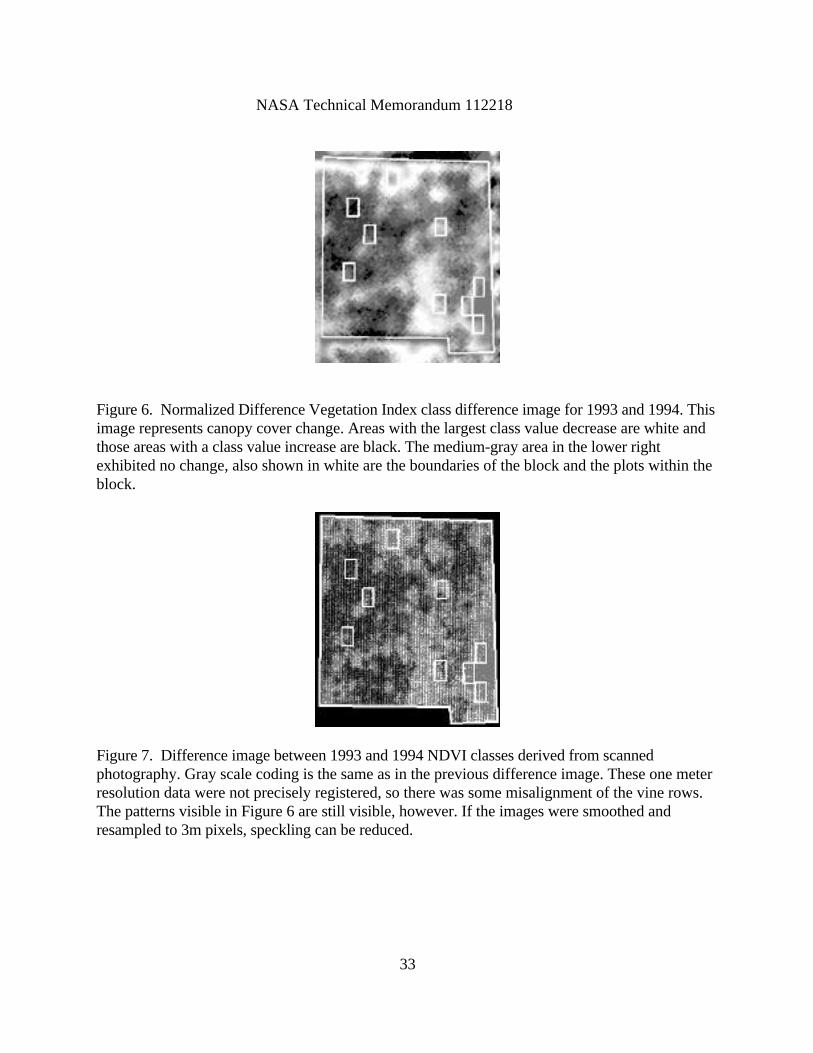
A difference image was generated for block I (Figure 6) to spectrally compare the images.

Image differencing was accomplished by subtracting 1994 NDVI class image from the 1993 class

image. An extensive area, in the middle of the vineyard block indicated a significant NDVI

decrease associated with the spread of phylloxera. The dark gray areas on the left side of the


14

vineyard block indicate canopy cover increases. This image also exhibited large decreases centered

on the areas with lower class values in 1993, such as at the upper middle of the block (Figure 3).

NDVI analysis was also performed with the scanned color infrared photographs from

block I. Comparison of the 1993 NDVI classes with the 1993 pruning weights resulted in an R2

of 0.64. Comparisons of the 1994 classes and 1994 weights resulted in an R2 of 0.90. NDVI

values from the 1993 scanned photograph compared to the 1993 pruning weights resulted in an

R2 of 0.61. The 1994 digitized photo generated NDVI values and pruning weights had an R2 of

0.91. We surmise this indicated that scanned aerial photography may produce similar results to

digitally acquired imagery if used with the classification procedure outlined above. A difference

image was also computed for these photographs (Figure 7) with patterns similar to those in

Figure 6, but with a higher spatial resolution.

Proximity Analysis

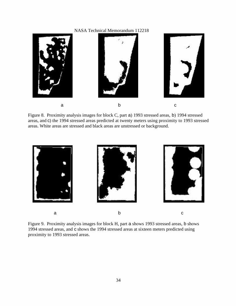
Areas that were conspicuously damaged by phylloxera for each year were identified on

the imagery to determine an NDVI class threshold and generate a vegetation stress image as

follows. For each year the classified NDVI image was combined with the corresponding false

color infrared (CIR) image to visually determine a threshold class number for 1993 and 1994.

Pixels below this threshold were considered to represent stressed vegetation in the NDVI

classified images. For the four blocks (C, H, I, and J), the same threshold was applied to each

based on similarities in age, vine and row spacing, and trellis type. The threshold may require

modification from block to block due to differences in vine canopy caused by various trellis

types, vine spacings, or age differences. For example, a block with wider row spacing would have

lower NDVI values than a block with narrower rows, due to the increase in soil area being sensed,

although the vine canopy may exhibit similar health characteristics. To compensate for this


15

difference, the threshold value may need to be lowered for a less densely planted block. The

classified images for each year were then each recoded into a binary image exhibiting only stressed

and non-stressed areas (parts a and b of Figures 8-11).

A proximity search, a GIS function, was performed for each of the 1993 stress images out

to 40 m from the edge of the stressed areas. In the resulting proximity image the value at each

pixel is the distance from the stressed areas, where areas inside the stressed areas have a distance

value of zero. Starting with a distance value of zero, the search image was iteratively recoded into

a series of binary images, where the pixels within the specified distance from the 1993 stressed

pixels were predicted to be stressed in 1994. This resulted in a phylloxera stress prediction for

the following year. The vineyard manager can use this predictive tool to prepare for lower yields

or plot eradication for that block.

Finally, the stressed areas at each distance were compared to each of the 1994 stress

images to determine the best predictive match. The recoded image was compared with the 1994

stress image by calculating the percentage of mismatched pixels, or error, at each distance. There

were two error components: commission and omission. This gave four occurrence possibilities,

since a given pixel could be stressed or non-stressed in each year. The two error components

were: (1) the area that was not predicted but was stressed (error of omission) and (2) the area

that was predicted but was not stressed (error of commission). These two counts were totaled

and divided by the total number of pixels in each block to derive the error estimates of phylloxera

spread prediction.

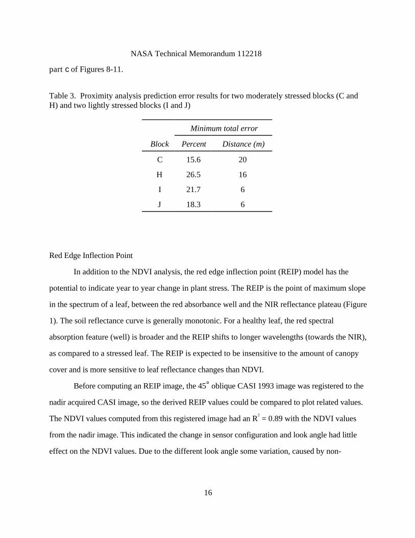
The distance of minimum error was the spread rate from 1993 to 1994 for that block. The

percentage errors for the four blocks are shown in Table 3. These data demonstrate that the

spread rate of the stressed areas was higher for the blocks that were already moderately stressed,

consistent with previous research (Wildman, 1983). The predicted stress images are shown in


16

part c of Figures 8-11.

Table 3. Proximity analysis prediction error results for two moderately stressed blocks (C andH) and two lightly stressed blocks (I and J)

Minimum total error

Block Percent Distance (m)

C 15.6 20

H 26.5 16

I 21.7 6

J 18.3 6

Red Edge Inflection Point

In addition to the NDVI analysis, the red edge inflection point (REIP) model has the

potential to indicate year to year change in plant stress. The REIP is the point of maximum slope

in the spectrum of a leaf, between the red absorbance well and the NIR reflectance plateau (Figure

1). The soil reflectance curve is generally monotonic. For a healthy leaf, the red spectral

absorption feature (well) is broader and the REIP shifts to longer wavelengths (towards the NIR),

as compared to a stressed leaf. The REIP is expected to be insensitive to the amount of canopy

cover and is more sensitive to leaf reflectance changes than NDVI.

Before computing an REIP image, the 45° oblique CASI 1993 image was registered to the

nadir acquired CASI image, so the derived REIP values could be compared to plot related values.

The NDVI values computed from this registered image had an R2 = 0.89 with the NDVI values

from the nadir image. This indicated the change in sensor configuration and look angle had little

effect on the NDVI values. Due to the different look angle some variation, caused by non-


17

Lambertian reflectance from the canopy was expected. REIP images were generated by fitting

pixel values from channels 4 - 8 (680 - 788 nm) to a third order polynomial and solving for the

location of maximum slope (Baret et al., 1992). The following form for radiance as a function of

wavelength was used for curve fitting:

L(λx) = a λx3 + b λx

2+ c λx + d,

where L(λx) is the radiance in channel x centered at wavelength λx. The set of equations for all of

the channels was then solved for the coefficients a, b, c, and d at each pixel. Taking the second

derivative and setting it to zero resulted in the following equation for the REIP wavelength, REIP:

REIP = -b / 3a

The REIP wavelengths were calculated using radiance values for each pixel. For example,

given radiance values 33, 50, 78, 87, and 88 W/m2.sr.µm, for the channels centered at 681, 710,

737, 747, and 788 nm respectively, the equation for radiance was estimated using least squares

regression:

L(λx) = -0.00017557 λx3 + 0.38163 λx

2 - 275.45 λx + 66077,

where the REIP was 724.55 nm.

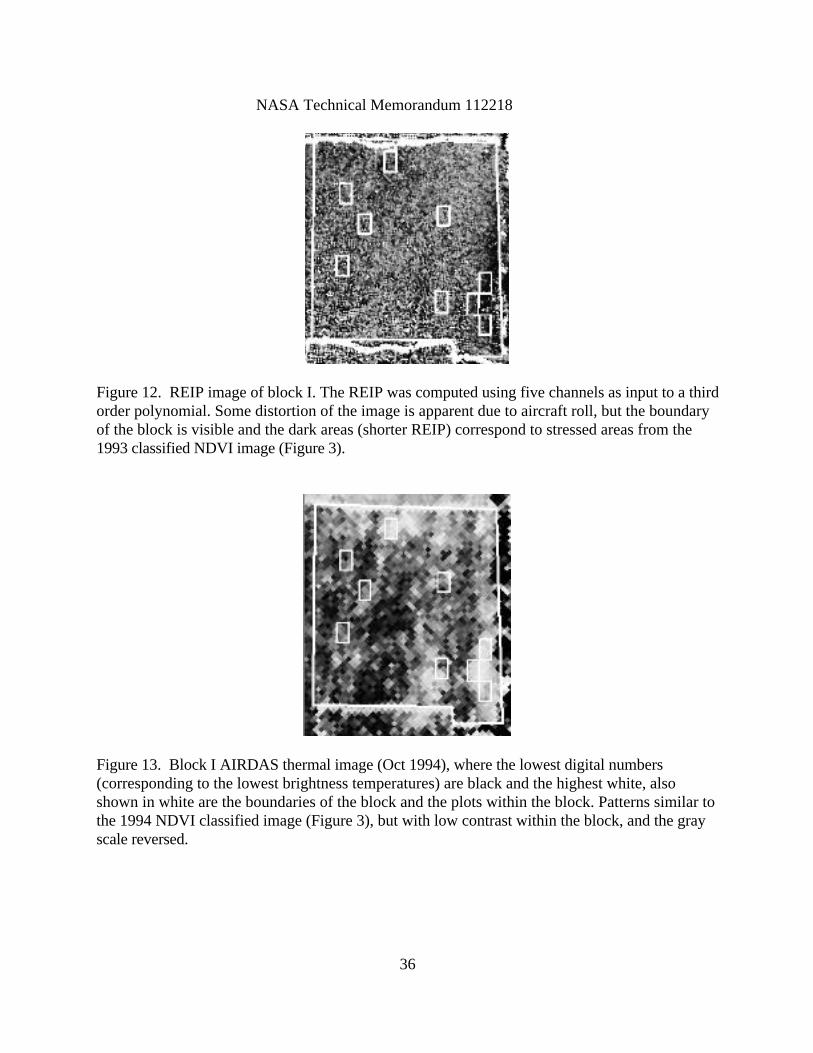
The mean REIP's for the plots are shown in Table 4 and the REIP image is shown in

Figure 12. Though the REIP images were noisy, the coefficients of determination with mean

REIP per plot were high: 0.72 with pruning weight, 0.83 with oblique NDVI, 0.89 with nadir

NDVI, and 0.88 with (nadir) NDVI class. The stronger relationship between pruning weights and

REIP, versus pruning weights and NDVI, may be due to the difference in viewing geometry or

the increased sensitivity of the REIP.


18

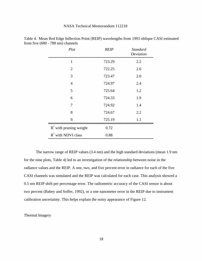
Table 4. Mean Red Edge Inflection Point (REIP) wavelengths from 1993 oblique CASI estimatedfrom five (680 - 788 nm) channels

Plot REIP StandardDeviation

1 723.29 2.2

2 722.25 2.6

3 723.47 2.0

4 724.97 2.4

5 725.64 1.2

6 724.33 1.9

7 724.92 1.4

8 724.67 2.2

9 725.19 1.1

R2 with pruning weight 0.72

R2 with NDVI class 0.88

The narrow range of REIP values (3.4 nm) and the high standard deviations (mean 1.9 nm

for the nine plots, Table 4) led to an investigation of the relationship between noise in the

radiance values and the REIP. A one, two, and five percent error in radiance for each of the five

CASI channels was simulated and the REIP was calculated for each case. This analysis showed a

0.5 nm REIP shift per percentage error. The radiometric accuracy of the CASI sensor is about

two percent (Babey and Soffer, 1992), or a one nanometer error in the REIP due to instrument

calibration uncertainty. This helps explain the noisy appearance of Figure 12.

Thermal Imagery


19

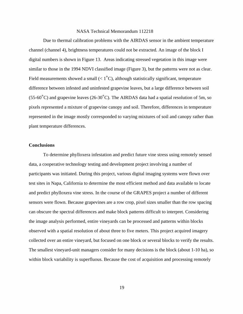
Due to thermal calibration problems with the AIRDAS sensor in the ambient temperature

channel (channel 4), brightness temperatures could not be extracted. An image of the block I

digital numbers is shown in Figure 13. Areas indicating stressed vegetation in this image were

similar to those in the 1994 NDVI classified image (Figure 3), but the patterns were not as clear.

Field measurements showed a small (< 1°C), although statistically significant, temperature

difference between infested and uninfested grapevine leaves, but a large difference between soil

(55-60°C) and grapevine leaves (26-30°C). The AIRDAS data had a spatial resolution of 5m, so

pixels represented a mixture of grapevine canopy and soil. Therefore, differences in temperature

represented in the image mostly corresponded to varying mixtures of soil and canopy rather than

plant temperature differences.

Conclusions

To determine phylloxera infestation and predict future vine stress using remotely sensed

data, a cooperative technology testing and development project involving a number of

participants was initiated. During this project, various digital imaging systems were flown over

test sites in Napa, California to determine the most efficient method and data available to locate

and predict phylloxera vine stress. In the course of the GRAPES project a number of different

sensors were flown. Because grapevines are a row crop, pixel sizes smaller than the row spacing

can obscure the spectral differences and make block patterns difficult to interpret. Considering

the image analysis performed, entire vineyards can be processed and patterns within blocks

observed with a spatial resolution of about three to five meters. This project acquired imagery

collected over an entire vineyard, but focused on one block or several blocks to verify the results.

The smallest vineyard-unit managers consider for many decisions is the block (about 1-10 ha), so

within block variability is superfluous. Because the cost of acquisition and processing remotely


20

sensed digital imagery is inversely proportional to the pixel size, three to five meters is a good

tradeoff between cost and spatial resolution.

The use of the same sensor for each flight, while not necessary, would greatly simplify

data processing and improve confidence in the derived image products. If the spatial resolution

between sensors is different, the resolution of the sensors has to be matched by image analysis

techniques. Spectral values between different systems do not have to match; as long as the data

sets are not significantly different, because clustering each NDVI image and the NDVI itself

compensates for differences in atmospheric conditions.

The mean spectral-class value per plot was found to be highly correlated to the pruning

weight per plot for each year. The correlation between pruning weight and mean NDVI class per

plot was higher than the correlation between pruning weight and mean NDVI value per plot (R2 =

0.76 compared to 0.66). Good results with digitally acquired imagery were achieved without

sensor calibration and atmospheric correction by using spectrally classified data to examine

relative differences in canopy cover per year. Preliminary results indicate this classification

procedure should provide improved results with scanned photography as well as digitally

acquired imagery.

Histograms of the spectrally classified, digitally acquired, images for block I also showed

a change from a homogeneous block in 1993, with a sharply peaked histogram, to a relatively flat

histogram, non-uniform block, in 1994. If an unsupervised classification procedure is used, then

the classified images can be ground truthed or compared to other imagery to determine the

relationship between classes, canopy cover, and damage level. This information can be used to

determine a threshold for classes of stressed or conspicuously damaged vegetation. The effect of

different trellising types or row spacing on NDVI was not explicitly investigated, but the

approach should provide a good indication of relative differences within a given field.


21

Proximity analysis provided a method of estimating the next year's phylloxera damage.

Given some initial conspicuously damaged areas within a block, a proximity spread, based on

region growing from the existing clusters, can provide an estimate of future damage. Since new

phylloxera infestation locations within a block occur, in addition to spreading from an existing

infestation location, and the spread rate within a block was not the same across a block,

prediction error was approximately 20%. For block I (a five-hectare block), the damaged area was

1.1 ha in 1993, 2.2 ha in 1994, and the estimated damaged area in 1994 was 1.8 ha, with an error

of about one-hectare. Phylloxera are also usually well established by the time a damaged area is

large enough to be considered a center of growth. By the following year the block will be

moderately or heavily damaged, and combined with the large prediction error, a prediction

beyond one year is not practical. Spread analysis does, however, provide a tool for exploring

different scenarios of spread rates and growth centers. Insufficient testing was done to determine

if a single growth rate could be uniformly applied to vineyard blocks and still obtain reasonably

accurate predictions, but the results of this study suggest different growth rates are needed.

Red edge inflection point (REIP) results and thermal imagery for the plots were

promising, but less meaningful than the NDVI products. The REIP results agreed well with the

pruning weights and NDVI class results, but they require special narrow spectral bandpass filters

along the red edge that are not commonly available. Due to the narrow range (a few nanometers),

REIP analysis also requires detailed spectral and radiometric calibration throughout the image.

This is a current problem with CCD (charge coupled device) arrays, and the data need to be

stable if multi-temporal studies are to be practical. Patterns, indicating stressed vegetation, were

present in the thermal imagery, but were not as distinct as in the NDVI imagery. Leaf

temperature was difficult to measure due to the open canopy. As an indication of canopy cover

and vegetative health, the easily derived NDVI and following classified imagery were easier to


22

interpret than the REIP or the thermal imagery.

Commercial airborne imagery acquisition services exist to provide the data needed for

generating NDVI products. Only a red and a near infrared channel are needed to compute an

NDVI, but multiple channels in the red to near-infrared spectral region are needed for computing

the REIP. A thermal sensor is needed to acquire thermal imagery. In the next few years (1998)

satellites will provide commercial multispectral data with four-meter spatial resolution. Through

procedures such as those outlined here, airborne imagery acquired in the visible and near-infrared

can complement vineyard managers' knowledge gained from conventional ground-based

techniques, aerial photography, and experience.

The imagery indicated plant stress due to phylloxera and other sources, such as water

stress. Airborne imagery can serve multiple roles in vineyard management. Multi-year imagery

can be used to help identify the type of stress if the growth pattern can be identified. The

benefits versus the costs of multiple flights per year are still unknown, but the information gained

from a single flight per year was considered worthwhile to the Mondavi vineyard management

team. Knowledge of the pattern change from year to year allows the vineyard manager to

intervene and apply remedial measures as well as provide data for financial forecasts.

Recommendations

To monitor the phylloxera infestation of a vineyard, digital multispectral imagery, should

be acquired at least once a year at full canopy, between mid-season and harvest. The imagery

should have a spatial resolution not to exceed three meters and the use of the same sensor

package for each data collection period is important. The data can be used to generate co-

registered, classified, NDVI data sets for multi-year comparisons. In classifying one block, five or

six spectral classes are sufficient, but ten to twelve should be used for an image of an entire


23

vineyard. A small number of classes makes image product interpretation easier, but some features

could be missed with too few classes. To avoid problems with changing amount of bare soil in the

imagery, a threshold should be used to eliminate low NDVI pixels.

Computer Facilities

All image processing described above was performed at the NASA Ames Research

Center's ECOSAT Computational Facility with ERDAS Imagine 8.20 (ERDAS, Inc., Atlanta,

GA) running under Solaris on a Sun Microsystems SPARCstation. The processing described here

used standard image processing routines available on a PC using any one of number of commonly

available geographic image processing software packages. More information about satellite image

processing, much of which also applies to aircraft imagery, including software sources, can be

found in the Satellite Imagery Frequently Asked Questions (FAQ) at

http://www.geog.nottingham.ac.uk/remote/satfaq.html.

Acknowledgments

Work to establish the plot size and locations and phylloxera levels within the plots was

performed by E. Weber (University of California Cooperative Extension Napa County), J. De

Benedictis (UC Davis), R. Baldy, and M. Baldy (both California State University Chico). GPS

data were collected by C. Bell (Johnson Controls World Services, NASA Ames Research Center,

currently California Department of Forestry through UC Davis) and B. Osborn (UC Davis,

currently Glen Ellen Carneros Winery). Pruning weights were courtesy of Robert Mondavi

Winery (D. Bosch). A. Bledsoe, D. Bosch (both Robert Mondavi Winery), and P. Freese (Wine

Grow) provided guidance throughout the project. Other contributors included D. Peterson, J.

Salute, and V. Vanderbilt (all NASA Ames Research Center). The work described in this paper


24

was performed at the NASA Ames Research Center under UPN 233-01-04-05 in fiscal years

1993 - 1995.

Project URL (Web Page Address)http://geo.arc.nasa.gov/sge/grapes/grapes.html


25

Appendix: Sensor Specifications

The sensors flown in the course of this project were summarized in Table 1, but this

appendix describes these sensors in more detail. The sensors were flown on aircraft platforms at

low, medium, and high altitudes and had a various spectral characteristics. Half of these were

charge-coupled device (CCD) sensors and the other half were scanners. Scanning sensors use a

linear array of photo detectors that measures the intensity of radiance within some wavelength

region as the sensor passes (or sweeps) over the landscape, while a CCD sensor uses an array of

detectors and takes a "snapshot" of the landscape.

Sensors measure radiant intensity at some wavelength range and have two types of

resolution: spatial and radiometric. The wavelength region of each sensor channel is determined

by the spectral response function of the wavelength filter, and the bandwidth of the filter at half

maximum value is the full width half maximum (FWHM). Spatial resolution was defined on page

5 as related to aircraft altitude, but this was just another way of describing a detector's

instantaneous field of view (IFOV), or angular width. Because a detector's IFOV is fixed, a change

in altitude changes the amount of landscape subtended by the detector. This quantity is

expressed in radians, where 1.0 r = π/180°, or usually in milliradians. The radiometric resolution

of these sensors was eight bits, except the CASI sensor with twelve bits and the AIRDAS sensor

with sixteen bits. Some of these sensors, like CASI, can be reconfigured for multiple purposes,

but Table A1 describes the configurations used with the GRAPES project.


26

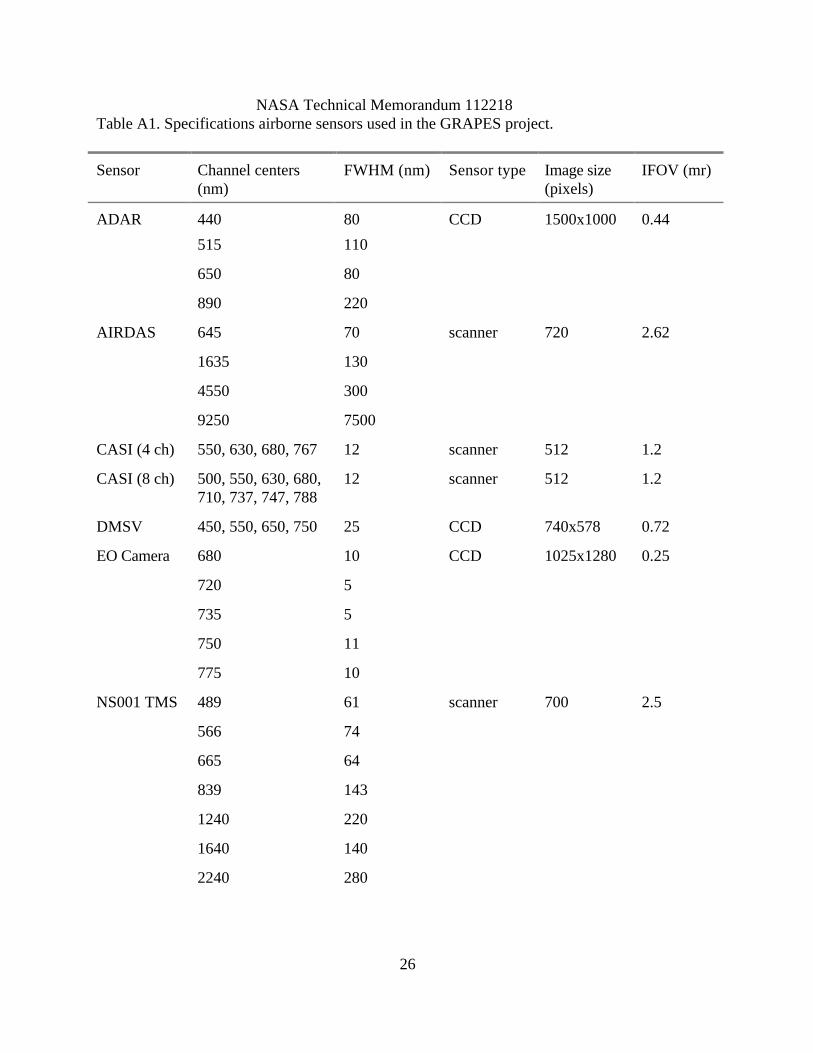
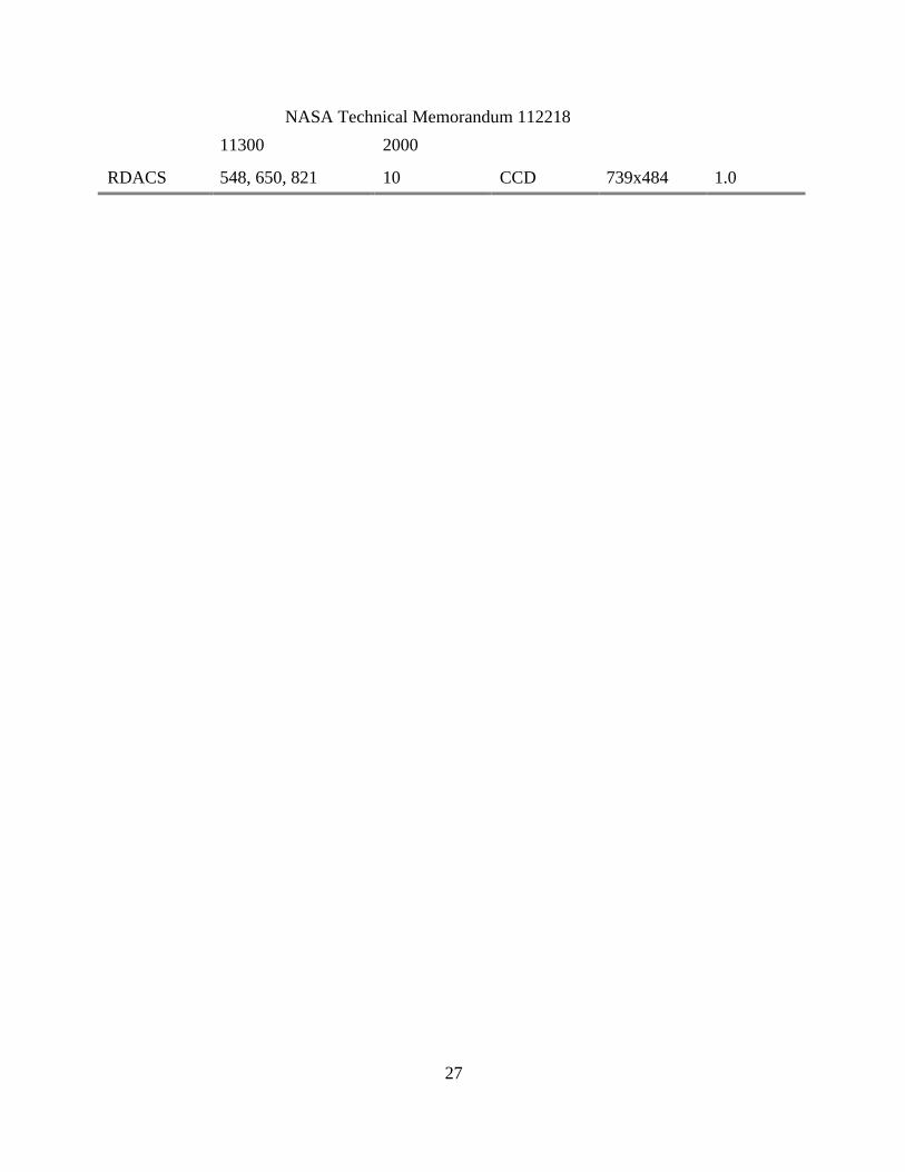
Table A1. Specifications airborne sensors used in the GRAPES project.

Sensor Channel centers(nm)

FWHM (nm) Sensor type Image size(pixels)

IFOV (mr)

ADAR 440 80 CCD 1500x1000 0.44

515 110

650 80

890 220

AIRDAS 645 70 scanner 720 2.62

1635 130

4550 300

9250 7500

CASI (4 ch) 550, 630, 680, 767 12 scanner 512 1.2

CASI (8 ch) 500, 550, 630, 680,710, 737, 747, 788

12 scanner 512 1.2

DMSV 450, 550, 650, 750 25 CCD 740x578 0.72

EO Camera 680 10 CCD 1025x1280 0.25

720 5

735 5

750 11

775 10

NS001 TMS 489 61 scanner 700 2.5

566 74

665 64

839 143

1240 220

1640 140

2240 280


27

11300 2000

RDACS 548, 650, 821 10 CCD 739x484 1.0


28

References

Ambrosia, V. G., J. A. Brass, J. B. Allen, E. A. Hildum, and R. G. Higgins. 1994. AIRDAS,development of a unique four channel scanner for natural disaster assessment. FirstInternational Airborne Remote Sensing Conference and Exhibition, Strasbourg, France, 11-15 September 1994.

Babey, S. and R. Soffer. 1992. Radiometric calibration of the compact airborne spectrographicimager (CASI). Canadian Journal of Remote Sensing 18(4):233-242.

Baret, F., S. Jacquemoud, G. Guyot, and C. Leprieur. 1992. Modeled analysis of the biophysicalnature of spectral shifts and comparison with information content of broad bands.Remote sensing of Environment 41:133-142.

Borstad Associates, Ltd. 1991. Low cost digital remote sensing using the Compact AirborneSpectrographic Imagery. Sidney, British Columbia, Canada: Borstad Associates, Ltd.

Duda R. and P. Hart. 1973. Pattern Classification and Scene Analysis. New York:John Wiley andSons, Inc.

Granett, J., A. Goheen, and L. Lider. 1987. Grape phylloxera in California. California Agriculture41(1):10-12.

Granett, J., J. De Benedictis, J. Wolpert, E. Weber, and A. Goheen. 1991. Deadly insect pestposes increased risk to north coast vineyards. California Agriculture 45(2):30-32.

Johnson, L. F., B. Lobitz, R. Armstrong, R. Baldy, E. Weber, J. De Benedictis, and D. Bosch.1996. Airborne imaging aids vineyard canopy evaluation. California Agriculture 50(4):14-18.

Lyon, R. J. P. 1994. SpecTerra digital multi-spectral video image data formats. Stanford, CA:SpecTerra Systems, Pty, Ltd.

Tucker, C. J. 1979. Red and photographic infrared linear combinations for monitoring vegetation.Remote Sensing of Environment 8:127-150.

Wildman, W. E., R. T. Nagaoka, and L. A. Lider. 1983. Monitoring spread of grape phylloxera bycolor infrared aerial photography and ground investigation. American Journal of Enologyand Viticulture 34(2):83-94.


29

Figure 1. Example of leaf and soil spectra. The REIP is the point of maximum slope in thespectrum of a leaf. A healthy leaf has a broader spectral absorption in the red (680 nm) and REIPoccurs at a longer wavelength, as compared to a stressed leaf.


30

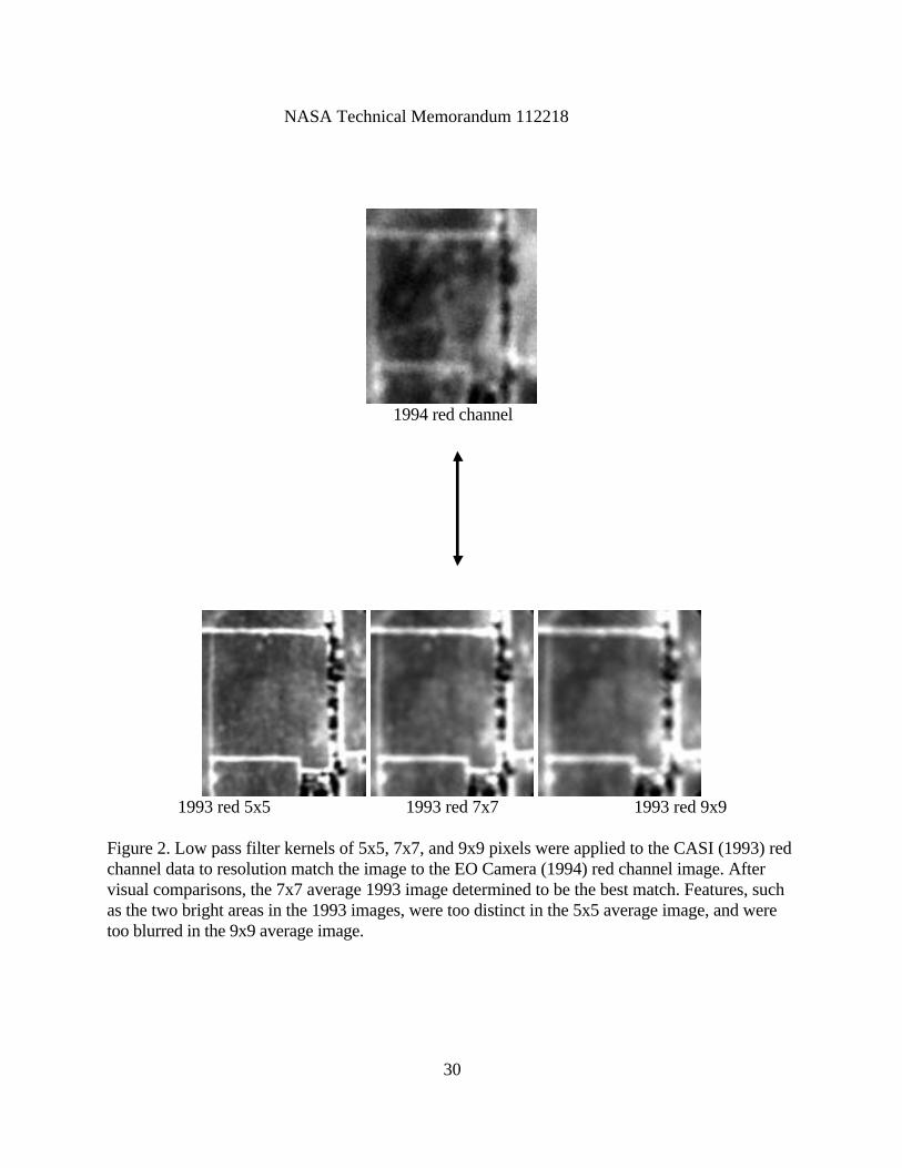
1994 red channel

1993 red 5x5 1993 red 7x7 1993 red 9x9

Figure 2. Low pass filter kernels of 5x5, 7x7, and 9x9 pixels were applied to the CASI (1993) redchannel data to resolution match the image to the EO Camera (1994) red channel image. Aftervisual comparisons, the 7x7 average 1993 image determined to be the best match. Features, suchas the two bright areas in the 1993 images, were too distinct in the 5x5 average image, and weretoo blurred in the 9x9 average image.


31

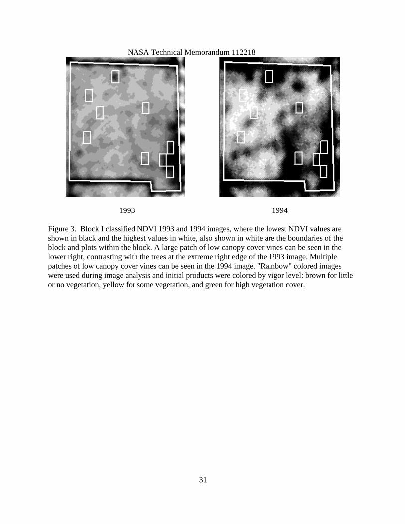
1993 1994

Figure 3. Block I classified NDVI 1993 and 1994 images, where the lowest NDVI values areshown in black and the highest values in white, also shown in white are the boundaries of theblock and plots within the block. A large patch of low canopy cover vines can be seen in thelower right, contrasting with the trees at the extreme right edge of the 1993 image. Multiplepatches of low canopy cover vines can be seen in the 1994 image. "Rainbow" colored imageswere used during image analysis and initial products were colored by vigor level: brown for littleor no vegetation, yellow for some vegetation, and green for high vegetation cover.


32

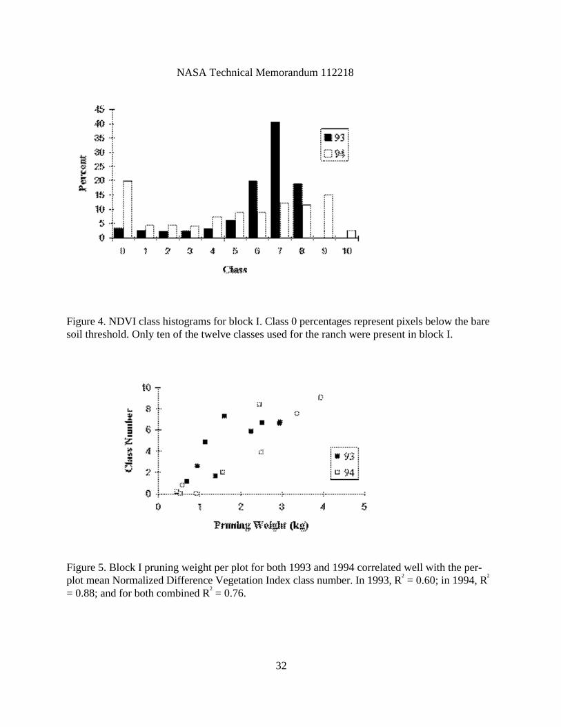
Figure 4. NDVI class histograms for block I. Class 0 percentages represent pixels below the baresoil threshold. Only ten of the twelve classes used for the ranch were present in block I.

Figure 5. Block I pruning weight per plot for both 1993 and 1994 correlated well with the per-plot mean Normalized Difference Vegetation Index class number. In 1993, R2 = 0.60; in 1994, R2

= 0.88; and for both combined R2 = 0.76.


33

Figure 6. Normalized Difference Vegetation Index class difference image for 1993 and 1994. Thisimage represents canopy cover change. Areas with the largest class value decrease are white andthose areas with a class value increase are black. The medium-gray area in the lower rightexhibited no change, also shown in white are the boundaries of the block and the plots within theblock.

Figure 7. Difference image between 1993 and 1994 NDVI classes derived from scannedphotography. Gray scale coding is the same as in the previous difference image. These one meterresolution data were not precisely registered, so there was some misalignment of the vine rows.The patterns visible in Figure 6 are still visible, however. If the images were smoothed andresampled to 3m pixels, speckling can be reduced.


34

a b c

Figure 8. Proximity analysis images for block C, part a) 1993 stressed areas, b) 1994 stressedareas, and c) the 1994 stressed areas predicted at twenty meters using proximity to 1993 stressedareas. White areas are stressed and black areas are unstressed or background.

a b c

Figure 9. Proximity analysis images for block H, part a shows 1993 stressed areas, b shows1994 stressed areas, and c shows the 1994 stressed areas at sixteen meters predicted usingproximity to 1993 stressed areas.


35

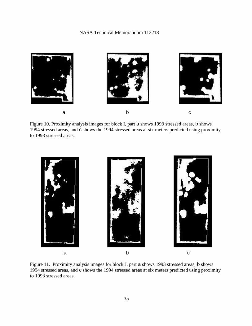
a b c

Figure 10. Proximity analysis images for block I, part a shows 1993 stressed areas, b shows1994 stressed areas, and c shows the 1994 stressed areas at six meters predicted using proximityto 1993 stressed areas.

a b c

Figure 11. Proximity analysis images for block J, part a shows 1993 stressed areas, b shows1994 stressed areas, and c shows the 1994 stressed areas at six meters predicted using proximityto 1993 stressed areas.


36

Figure 12. REIP image of block I. The REIP was computed using five channels as input to a thirdorder polynomial. Some distortion of the image is apparent due to aircraft roll, but the boundaryof the block is visible and the dark areas (shorter REIP) correspond to stressed areas from the1993 classified NDVI image (Figure 3).

Figure 13. Block I AIRDAS thermal image (Oct 1994), where the lowest digital numbers(corresponding to the lowest brightness temperatures) are black and the highest white, alsoshown in white are the boundaries of the block and the plots within the block. Patterns similar tothe 1994 NDVI classified image (Figure 3), but with low contrast within the block, and the grayscale reversed.

Documents

Grapevine Remote sensing Analysis of Phylloxera Early ... · Remote sensing Analysis of Phylloxera ... the California State University, and Robert Mondavi Winery examined the application