NASA Technical Memorandum 112218

Grapevine Remote SensingAnalysis of Phylloxera EarlyStress (GRAPES): RemoteSensing Analysis Summary

Brad Lobitz, Johnson Controls World Services, Inc., Ames Operation�Ames Research Center,Moffett Field, California

Lee Johnson, Johnson Controls World Services, Inc., Ames Operation�Ames Research Center,Moffett Field, CaliforniaChris Hlavka, Ames Research Center, Moffett Field, CaliforniaRoy Armstrong, Johnson Controls World Services, Inc., Ames Operation/Ames Research Center,Moffett Field, Califomia

Cindy Bell, Johnson Controls World Services, Inc., Ames Operation�Ames Research Center,Moffett Field, California

December 1997

National Aeronautics andSpace Administration

Ames Research CenterMoffett Field, California 94035-1000

GRAPEVINE REMOTE SENSING ANALYSIS OF PHYLLOXERA EARLY

(GRAPES): REMOTE SENSING ANALYSIS SUMMARY

Brad Lobitz I , Lee Johnson 2, Chris Hlavka 3, Roy Armstrong 4, and Cindy Bell 5

STRESS

SUMMARY

This document describes image processing analysis applied to high spatial resolution airborne imagery

acquired in California's Napa Valley in 1993 and 1994 as part of the Grapevine Remote sensing

Analysis of Phylloxera Early Stress (GRAPES) project. Investigators from NASA, the University of

California, the California State University, and Robert Mondavi Winery examined the application of

airborne digital imaging technology to vineyard management, with emphasis on detecting the

phylloxera infestation in California vineyards, Phylloxera infestation is a significant problem because

the root louse causes vine stress that leads to grapevine death in three to five years. Eventually the

infested areas must be replanted with resistant rootstock. Visual symptoms of phylloxera infestation

include leaf chlorosis, vine size reduction, and collapse of fruit tissue during the growing season.

Increased leaf temperatures have also been hypothesized for affected vines. Early detection of

infestation and changing cultural practices to compensate for vine damage can minimize crop financial

losses from damage and replanting. Vineyard managers need improved information to decide where

and when to replant fields or sections of fields.

Multi-year airborne images of a vineyard were spatially co-registered so annual relative changes in leaf

area due to phylloxera infestation could be located. Image processing analysis was applied to data from

the Compact Airborne Spectrographic Imager (CASI, imagery acquired in 1993) and the Electro-Optic

Camera (EO Camera, imagery acquired in 1994). Changes were determined by using information

obtained from computing Normalized Difference Vegetation Index (NDVI) images. -As the canopy leaf

area of infested regions decreased, these regions became increasingly non-uniform. Infestation spread

was also projected in advance using proximity analysis, a geographic information system (GIS)

technique. Two other methods of monitoring vineyards through imagery were also investigated:

optical sensing of the Red Edge Inflection Point (REIP), and thermal sensing. These did not convey

the stress patterns as well as the NDVI imagery and require specialized sensor configurations. NDVI-

derived products are recommended for monitoring phylloxera infestations.

l Johnson Controls World Services, Inc., Ames Operation

2Johnson Controls World Services, Inc., Ames Operation (currently Institute Earth Systems Science & Policy, California State

University, Monterey Bay)

3NASA Ames Research Center

4Johnson Controls World Services, Inc., Ames Operation (currently Dept. of Marine Sciences, University of Puerto Rico)

5Johnson Controls World Services, Inc., Ames Operation (currently Pacific Meridian Resources, Emeryville, CA)

INTRODUCTION

Phylloxera (Daktulosphaira vitifoliae Fitch) affects a number of the grape growing counties in

California and is currently a severe problem in Napa and Sonoma Counties. The parasitic action of this

root louse causes leaf chiorosis, decreases shoot and leaf growth and fruit yield, and leads to vine

death three to five years from onset. Once established, the infestation spreads quickly through a

vineyard. The grapevines' deep rooting pattern makes pesticides ineffective and there is no known

biological control (refs. 1 & 2).

Changing cultural practices, such as adjusting pruning severity or changing the amount of irrigation,

are sometimes used to prolong fruit production, but there is little the grape grower can do to combat

phylloxera, except replant on phylloxera-resistant rootstock. As the infestation spreads, the grape yield

decreases each year, until the yield is too low justify the maintenance costs and the vines are plowed

up. Replanting is expensive, and the field will also be out of production for a number of years before

the newly planted vines bear fruit.

The GRAPES project was a collaboration between NASA Ames Research Center, the University of

California Davis, the University of California Cooperative Extension, California State University

Chico, and Robert Mondavi Winery (Oakville, CA). The project was developed to demonstrate the use

of remotely sensed data for vineyard management, with emphasis on monitoring phylloxera

infestation, for example, using remotely sensed data to help decide when to replant a phylloxerainfested field.

Some vineyard manager_ have used aerial photography to study phylloxera spread (ref. 3). The

GRAPES project incorporated airborne digital imaging systems with subsequent image processing and

analysis to enhance information content with respect to canopy size (ref. 4). This report summarizes

methodology used to generate annual imagery for vineyard managers to monitor the spread of

phylloxera in a Mondavi vineyard. This methodology could be applied to digitally acquired imagery

and to film-based traditional aerial photography that has been scanned into digital form. Satellite

images acquired by the Landsat Thematic Mapper (TM) and Satellite Pour l'Observation de la Terre

(SPOT) were also purchased, but were used for valley wide analysis and not at the vineyard or block

scale. (A block is the smallest management unit within a vineyard.) This document also describes the

image processing analysis applied to high spatial resolution airborne imagery acquired in California's

Napa Valley in 1993 and 1994. Results of the analysis indicate the procedures used offer tangible

benefits to growers.

STUDY SITE AND GROUND DATA

Airborne digital data were acquired over the study site, ToKalon Ranch (a vineyard owned and

managed by the Robert Mondavi Winery), in 1993 and most of Napa Valley, including ToKalon and

two other Mondavi vineyards, Carneros and Oak Knoll, in 1994. ToKalon ranch lies on the West edge

of the valley floor and is surrounded on the other three sides by other vineyards. The ToKalon soils

are mainly Bale loam and clay loam with 0--2% slope, with some Bale clay loam with 2-5% slope and

some Coombs gravelly loam with 0-2% slope. The southern portion of the ranch is Clear Lake clay

(2-5% slope). Images from 1993 and 1994 covering all of ToKalon Ranch were processed, but this

report focuses on one five-hectare block (denoted as block I in the following discussion) within

ToKalon.Block I consistedof cabemetsauvignongrapevinesonAXR-1 rootstockwith four-meterrow spacingplantedprimarily in ClearLakeclaysoil.Theanalysisof thisblockwasusedto illustratethetypeof informationthatcanbegeneratedfor anentirevineyard.

Nineplotswithin block I wereusedfor collectingfield data(pruningweights,phylloxeracounts,andleaf samples).Theseplotswerechosenbasedon 1992aerialcolor infraredphotographyandapre-growingseasonphylloxerastudy.Interpretationof thecolorinfraredphotosprovidedlocationsofinfestedareas.Infestationlevelswerethenconfirmedbyrootdiggingin thefield.Thenineplotsconsistedof threeplotseachof uninfested,mildly infested,andseverelyinfestedvines.Eachplotcontainedforty vines.At theendof eachgrowingseason(January),Mondaviprunedthevinesandweighedvegetativematerial.Infraredtemperatureswerealsocollectedin thefield, usingahandheldinfraredthermometer,from five representativeplots,soil, androadsin 1994.Thesedatawereusedtosupportairbornethermalinfrareddatacollection.

AIRCRAFT DATA

Aerial photography (acquired by Ames Research Center's C-130 and ER2 aircraft) and digital imagery

from a variety of airborne sensors were used during the GRAPES project. Several airborne sensors

with different specifications and spectral characteristics were used to investigate block monitoring

capabilities and to test the utility of the digital image processing methods.

The airborne sensors used included: Airborne Data Acquisition and Registration (ADAR), Airborne

Infrared Disaster Assessment System (AIRDAS), CASI, Digital Multi-Spectral Video (DMSV), EO

Camera, NS001 Thematic Mapper Simulator (TMS), and Real Time Digital Airborne Camera System

(RDACS). Each of these sensors can be used to acquire image data at different spatial, spectral, and

radiometric resolutions. Spatial resolution, or ground resolution, is the size of the smallest area

element that can be detected for the image. Spatial resolution, referred to as pixel size, depends on the

sensor platform (aircraft) collection altitude. For example, the CASI sensor can be used to acquire

image data at spatial resolutions between 0.6 m and 10 m. At 1200 m altitude, the CASI system yields

a pixel size of 1.6 m (rounded to 2 m in this report) and at 450 m, 0.6 m. The total area imaged,

therefore, decreases with decreasing aircraft altitude. Below some limiting height the sensor systems

cannot acquire and store data fast enough to provide continuous ground coverage. The AIRDAS

(Ames Research Center) sensor, which was designed for fire monitoring, has two thermal infrared

channels (ref. 5). The AIRDAS low temperature, thermal channel (9250 nm center wavelength) was

the most interesting for the GRAPES project, because it was used to determine surface (brightness)

temperatures. The CASI can be used to collect data in spatial mode and spectral mode. In the CASrs

spatial mode the sensor functions as a push-broom imager with up to 15 bands and in spectral mode

the sensor operates like a group of spectrometers (1.8 nm spectral resolution) sweeping the flight path

(ref. 6). Only the spatial mode with four or eight channels and a resampled spatial resolution of about

2.0 m were used for the project. The four channel configuration was used to provide false color

infrared imagery and the eight channel configuration provided data along the red edge of the vegetation

reflectance curve, figure 1. The DMSV had four similar channels (ref. 7). The EO Camera, flown at an

altitude of 20 km aboard the NASA ER-2, has a nominal spatial resolution of five meters and was

flown with five channels. The NS001 TMS has eight channels, was flown aboard the NASA C-130

with a spatial resolution of three to five meters. Seven of these channels correspond to the TM

instrument channels. The RDACS has three cameras with narrow band filters (about ten nanometers).

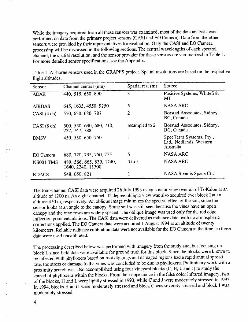
While the imageryacquiredfrom all thesesensorswasexamined,mostof thedataanalysiswasperformedondatafrom theprimaryprojectsensors(CASI andEOCamera).Datafrom theothersensorswereprovidedby theirrepresentativesfor evaluation.Only theCASI andEOCameraprocessingwill bediscussedin thefollowingsections.Thecentralwavelengthsof eachspectralchannel,thespatialresolution,andthesensorproviderfor thesesensorsaresummarizedin Table1.Formoredetailedsensorspecifications,seetheAppendix.

Table 1.Airbornesensorsusedin theGRAPESproject.Spatialresolutionsarebasedon therespectiveflight altitudes.

i

Sensor -i_imnnel centers (nm) Spaiiai res. (m) Source

ADAR 440, 515, 650, 890 3

AIRDAS 645, 1635, 4550, 9250 5

CASI (4 ch) 550, 630, 680, 787 2

CASI (8 ch) 500, 550, 630, 680, 710, resampled to 2737, 747, 788

DMSV 450, 550, 650, 750 1

EO Camera 680, 720, 735, 750, 775 5

NS001 TMS 489, 566, 665, 839, 1240, 3 to 51640, 2240, 11300

RDACS 548, 650, 821 1ii

Positive Systems, WhitefishMT

NASA ARC

Borstad Associates, Sidney,BC, Canada

Borstad Associates, Sidney,BC, Canada

SpecTerra Systems, Pty.,Ltd., Nedlands, WesternAustralia

NASA ARC

NASA ARC

NASA Stennis Space Ctr.

The four-channel CASI data were acquired 26 July 1993 using a nadir view over all of ToKalon at an

altitude of 1200 m. An eight-channel, 45 degree oblique view was also acquired over block I at an

altitude 450 m, respectively. An oblique image minimizes the spectral effect of the soil, since the

sensor looks at an angle to the canopy. Some soil was still seen because the vines have an open

canopy and the vine rows are widely spaced. The oblique image was used only for the red edge

inflection point calculations. The CASI data were delivered as radiance data, with no atmospheric

corrections applied. The EO Camera data were acquired 1 August 1994 at an altitude of twentykilometers. Reliable radiance calibration data were not available for the EO Camera at the time, so these

data were used uncalibrated.

The processing described below was performed with imagery from the study site, but focusing on

block I, since field data were available for ground truth for this block. Since the blocks were known to

be infested with phylloxera based on root diggings and damaged regions had a rapid annual spread

rate, the stress or damage to the vines was concluded to be due to phylloxera. Preliminary work with a

proximity search was also accomplished using four vineyard blocks (C, H, I, and J) to study the

spread of phylloxera within the blocks. From their appearance in the false color infrared imagery, twoof the blocks, H and I, were lightly stressed in 1993, while C and J were moderately stressed in 1993.

In 1994, blocks H and I were moderately stressed and block C was severely stressed and block J was

moderately stressed.

4

A 1993C-1301:6000scaleanda 1994ER2 1:32000scalephotographwerealsoavailablefor theToKalonRanchregion.Thephotographswerescannedto generatemultispectralimages,analogoustotheNIR, red,andgreenchannelsof anairbornescanner.Theeffectivepixel sizefor theseimagesafterregistrationwasonemeter.

PROCESSING AND RESULTS

There were several factors affecting the image analysis procedures: (1) the image data had to be in the

same map projection as, and spatially co-registered with, the other data layers used in the GRAPES

project (for example, soils, road network, hydrology); (2) the imagery was to be compared from year

to year; and (3) the data analysis procedures needed to be practical and applicable for procedural

repeatability and ease of use. The third factor required choosing a procedure providing results easily

comparable with the field data.

The second constraint was the most difficult to achieve. The data processing had to reconcile

differences in sensor characteristics and provide results that were not affected by differences in

viewing conditions. Several normalization schemes were tested to reconcile the data sets. The scheme

finally selected was chosen based on ease of implementation and validity of the results. The simplest

procedure was to match the spatial resolutions of the data, then classify the imagery based on the

NDVI values. This simple method provided sufficient results without complicated sensor calibration

and atmospheric correction models applied to the imagery.

Image Registration

The four-channel CASI imagery acquired in 1993 was used as the base date, while subsequent

airborne digital images were geo-registered to it. The ToKalon site data, consisting of three adjacent

passes, were mosaicked together into one image. The mosaicked image was registered to a Universal

Transverse Mercator (UTM) zone ten projection, with two-meter spatial resolution. This image

registration was accomplished using global positioning system (GPS) data points collected in the field.

These points were then located in the image and used as ground control points (GCPs). Finally, the

image was warped so the GCP's were in the correct positions relative to the UTM coordinate system.

Later images of the same area, such as the EO Camera imagery, were registered to this image. A

standard image to image transformation procedure was used. In this case the GCPs were pixel

locations in the CASI image and the equivalent pixel locations in the unregistered image.

Equalization of Spatial Resolution

The EO Camera imagery, acquired in 1994, was registered to the 1993 CASI imagery. The 1994 EO

Camera data had a nominal spatial resolution of five meters, while the CASI imagery had a spatial

resolution of two meters. The resolution difference was compounded by the EO Camera lens could not

be focused across all wavelength channels simultaneously, and consequently the channels, particularly

the red channel, were slightly out of focus. The 1994 image was registered to the 1993 image, while

adjusting for the pixel size (sampling interval) difference by resampling. Low pass (averaging) spatial

filters of various sizes were used to degrade the CASI and EO Camera near infrared (NIR) to the EO

Camera red spectral band spatial resolution. The best visual match was obtained with a 5x5 window

appliedto theEOCameraNIR bandanda7x7windowappliedto bothof theCASIchannels.ThisprocedurenormalizedtheEOCamerafocusingproblems,figure2.

Normalized Difference Vegetation Index Analysis

The NDVI was next applied to the imagery. The NDVI is defined as

NIR- redND VI =

NIR + red"

The NDV/highlights differences in vegetation canopy reflectance. Healthy vegetation has strong

absorbance characteristics in the red portion of the electromagnetic spectrum (EMS), while also

reflecting strongly in the NIR portion of the EMS. These properties are due to the interaction of light

with the chlorophyll in the plant tissue (fig. 1). Subtle changes in vegetation vigor or leaf chlorophyll

composition result in subtle alterations in absorbance and reflectance characteristics. These

characteristics are then highlighted in the NDVI. The index is near zero for bare soil, but can be close

to 1.0 for a dense, healthy canopy. The NDVI was used because it lessens the influence of solar

illumination, angular influences, slope, and viewing geometry. It performs consistently between

sensors, for different flights, and within the images. NDVI is also correlated to leaf area index (LAI),

or canopy leaf amount, and biomass (ref. 8). The index compensates for brightness differences and

highlights the spectral differences between pixels. Absolute NDVI's were not directly comparable

because of year-to-year differences in non-canopy variables and non-phylloxera related growth effects.

Non-canopy variables include calibration differences (the CASI data were calibrated to radiance versus

the raw EO Camera data), atmospheric conditions (weather conditions and aerosol concentration), and

solar illumination angle differences. Year-to-year plant growth differences could be also be a response

to other factors, including other plant stresses, changes in management practices, and increased rainfall

(that is, more irrigation) in I994. However, if the range of NDVI values within the images is

represented by classes, then relative values (classes) in the images from the same areas on different

dates can be compared. A small number of classes makes the images easier to interpret. Initially NDVI

data were assigned hues ranging from brown (bare soil), through yellow (small or stunted vines), to

dark green (vigorous growth). This approach showed damage patterns within the vineyard. Later,

images were coded using a rainbow (color spectrum) color coding due to the greater hue separation.

This scheme was preferred by the Mondavi vineyard manager and subsequently became the coding of

choice for the images.

Subjective comparisons of NDVI images of block I from 1993 and 1994 were difficult, so an

unsupervised classification was used to categorize block I and, later, the entire vineyard. An objective

method of determining class breaks was needed, so Iterative Self-Organizing Data Analysis

(ISODATA) (ref. 9), an unsupervised classification algorithm was used. Utilized with only one input

image band, the ISODATA routine determines the clusters within the range of pixel values in the image

using the number of clusters the user inputs. The ISODATA classification process begins by dividing

the range of values and using the midpoint of each breakpoint as the starting means for the number of

classes specified by the user. Each pixel is then assigned to the cluster that has the closest mean value

to the pixel value. Cluster means are then recomputed based on the pixels assigned to the clusters, and

the pixels are again assigned to clusters based on the new means. Eventually the means settle down

and the process terminates. When run on block I, six classes were used in the classification. This kept

thenumberof classesdowneaseof interpretation,while still representingtheimagevariation.For theentirevineyard,thisnumberwasdoubledto twelveclasses,sincetherewasmuchvariationin NDVIvaluesdueto differencesin vine maturity,trellis type,andvinespacingaswell asplantcondition.

A numberof vineyardblockswerepulledafterthe 1993dataacquisitionandsubsequently,largeareasof bare soil were evident in the 1994 imagery. These "soil" pixels would be over-represented in the

classes generated from the 1994 NDVI image. To equalize the distribution, the NDVI images were

visually compared with aerial photos and the false color infrared imagery to select an NDVI threshold

that masked out the nearly bare and bare soil pixels. Any pixels below the threshold (the soil) became

zero and were not considered in the classification routine. The thresholded image contained only

vegetated landscape elements and the range of NDVI values was therefore reduced. The proportion of

high NDVI pixels appeared stable, since those pixels were primarily trees along the streams, roads,

and hillside as well as the vigorous grapevines.

The ISODATA classification was performed to the filtered CASI (1993) and EO Camera (1994)

images. A common area covering the ToKalon vineyard was used in these steps for both years.

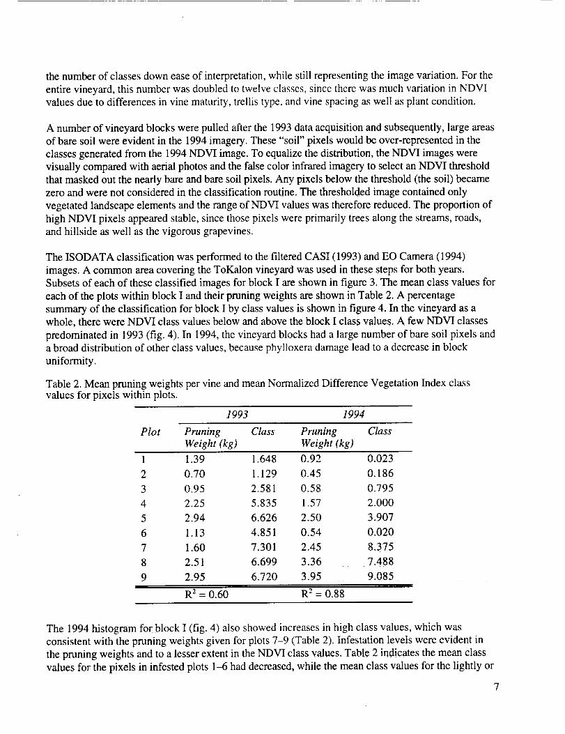
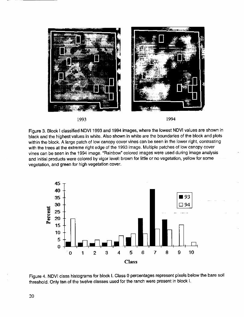
Subsets of each of these classified images for block I are shown in figure 3. The mean class values for

each of the plots within block I and their pruning weights are shown in Table 2. A percentage

summary of the classification for block I by class values is shown in figure 4. In the vineyard as a

whole, there were NDVI class values below and above the block I class values. A few NDVI classes

predominated in 1993 (fig. 4). In 1994, the vineyard blocks had a large number of bare soil pixels and

a broad distribution of other class values, because phylloxera damage lead to a decrease in block

uniformity.

Table 2. Mean pruning weights per vine and mean Normalized Difference Vegetation Index class

values for pixels within plots.

1993 1994

Plot Pruning Class Pruning Class

Weight (kg) Weight (kg)

1 1.39 1.648 0.92 0.023

2 0.70 1.129 0.45 0.186

3 0.95 2.581 0.58 0.795

4 2.25 5.835 1.57 2.000

5 2.94 6.626 2.50 3.907

6 1.13 4.851 0.54 0.020

7 1.60 7.301 2.45 8.375

8 2.51 6.699 3.36 7.488

9 2.95 6.720 3.95 9,085

R 2 = 0.60 R z = 0.88

The 1994 histogram for block I (fig. 4) also showed increases in high class values, which was

consistent with the pruning weights given for plots 7-9 (Table 2). Infestation levels were evident in

the pruning weights and to a lesser extent in the NDVI class values. Table 2 indicates the mean class

values for the pixels in infested plots 1--6 had decreased, while the mean class values for the lightly or

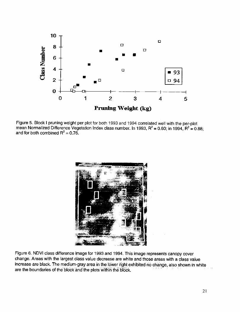
unaffectedplots(7, 8,and9) hadincreased.Classvalueswereplottedagainstpruningweight infigure5. CorrelationsbetweenthepruningweightsandeitherNDVI orclassvaluesweresimilar,thoughgreaterin 1994versus1993:R2wasabout0.60for 1993,0.86 for 1994.ThecorrelationbetweenpruningweightandNDVI classfor bothyearscombined(R2= 0.76)washigherthanthecorrelationbetweenall of thepruningweightswith all NDVI values(R2= 0.66).Therefore,classifyingtheimageryimprovedtherelationshipbetweenpruningweightsandNDVI. Similarimprovementoccurredwith theNDVI valueswhentheredandNIR channelswereradiometricallynormalizedbeforecomputingtheNDVI (resultsnotpresentedhere).

A differenceimagewasgeneratedfor blockI (fig. 6) to spectrallycomparetheimages.Imagedifferencingwasaccomplishedby subtracting1994NDVI classimagefrom the 1993classimage.Anextensivearea,in themiddleof thevineyardblock indicatedasignificantNDVI decreaseassociatedwith thespreadof phylloxera.Thedarkgrayareason theleft sideof thevineyardblockindicatecanopycoverincreases.This imagealsoexhibitedlargedecreasescenteredon theareaswith lowerclassvaluesin 1993,suchasattheuppermiddleof theblock(fig. 3).

NDVI analysiswasalsoperformedwith thescannedcolor infraredphotographsfromblock I.Comparisonof the 1993NDVI classeswith the 1993pruningweightsresultedin anR2of 0.64.Comparisonsof the 1994classesand1994weightsresultedin anR2of 0.90.NDVI valuesfrom the1993scannedphotographcomparedto the 1993pruningweightsresultedin anR2of 0.61.The 1994digitizedphotogeneratedNDVI valuesand pruning weights had an R 2of 0.91. We surmise this

indicated that scanned aerial photography may produce similar results to digitally acquired imagery if

used with the classification procedure outlined above. A difference image was also computed for these

photographs (fig. 7) with patterns similar to those in figure 6, but with a higher spatial resolution.

Proximity Analysis

Areas that were conspicuously damaged by phylloxera for each year were identified on the imagery to

determine an NDVI class threshold and generate a vegetation stress image as follows. For each year

the classified NDVI image was combined with the corresponding false color infrared (CIR) image to

visually determine a threshOld class number for 1993 and 1994. Pixels below this threshold were

considered to represent stressed vegetation in the NDVI classified images. For the four blocks (C, H,

I, and J), the same threshold was applied to each based on similarities in age, vine and row spacing,

and trellis type. The threshold may require modification from block to block due to differences in vine

canopy caused by various trellis types, vine spacings, or age differences. For example, a block with

wider row spacing would have lower NDVI values than a block with narrower rows, due to the

increase in soil area being sensed, although the vine canopy may exhibit similar health characteristics.

To compensate for this difference, the threshold value may need to be lowered for a less densely

planted block. The classified images for each year were then each recoded into a binary image

exhibiting only stressed and non-stressed areas (parts (a) and (b) of figs. 8-i 1).

A proximity search, a GIS function, was performed for each of the 1993 stress images out to 40 m

from the edge of the stressed areas. In the resulting proximity image the value at each pixel is thedistance from the stressed areas, where areas inside the stressed areas have a distance value of zero.

Starting with a distance value of zero, the search image was iteratively recoded into a series of binary

images, where the pixeis within the specified distance from the 1993 stressed pixels were predicted to

bestressedin 1994.Thisresultedin aphylloxerastresspredictionfor thefollowing year.Thevineyardmanagercanusethispredictivetool to preparefor loweryieldsor ploteradicationfor thatblock.

Finally, thestressedareasateachdistancewerecomparedto eachof the1994stressimagestodeterminethebestpredictivematch.Therecodedimagewascomparedwith the 1994stressimagebycalculatingthepercentageof mismatchedpixels,orerror,ateachdistance.Thereweretwo errorcomponents:commissionandomission.Thisgavefour occurrencepossibilities,sinceagivenpixelcouldbestressedor non-stressedin eachyear.Thetwoerrorcomponentswere:(1) theareathatwasnotpredictedbut wasstressed(errorof omission),and(2) theareathatwaspredictedbutwasnotstressed(errorof commission).Thesetwo countsweretotaledanddividedby thetotal numberofpixels in eachblock to derivetheerrorestimatesof phylloxeraspreadprediction.

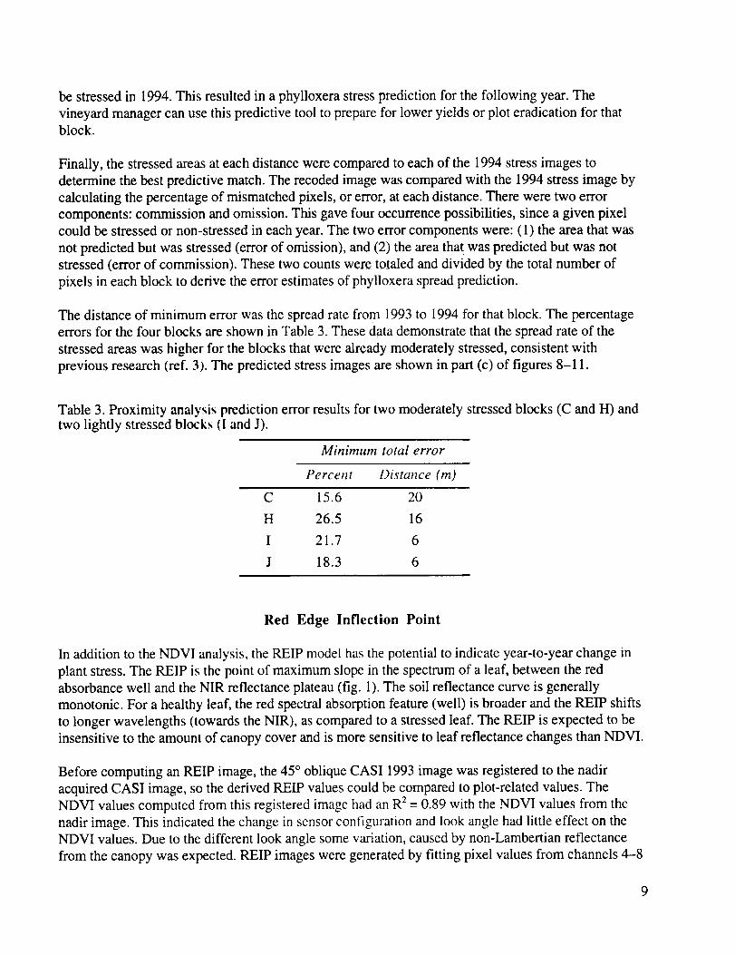
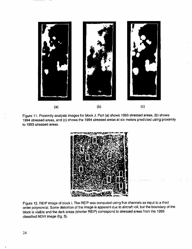
Thedistanceof minimumerrorwasthespreadratefrom 1993to 1994for thatblock.Thepercentageerrorsfor thefour blocksareshownin Table3.Thesedatademonstratethatthespreadrateof thestressedareaswashigherfor theblocksthatwerealreadymoderatelystressed,consistentwithpreviousresearch(ref. 3). The predicted stress images are shown in part (c) of figures 8-11.

Table 3. Proximity analysis prediction error results for two moderately stressed blocks (C and H) andtwo lightly stressed blocks (I and J).

Minimum total error

Percent Distance (m)

C 15.6 20

H 26.5 16

I 21.7 6

J 18.3 6

Red Edge Inflection Point

In addition to the NDVI analysis, the REIP model has the potential to indicate year-to-year change in

plant stress. The REIP is the point of maximum slope in the spectrum of a leaf, between the red

absorbance well and the NIR reflectance plateau (fig. 1). The soil reflectance curve is generally

monotonic. For a healthy leaf, the red spectral absorption feature (well) is broader and the REIP shifts

to longer wavelengths (towards the NIR), as compared to a stressed leaf. The REIP is expected to be

insensitive to the amount of canopy cover and is more sensitive to leaf reflectance changes than NDVI.

Before computing an REIP image, the 45 ° oblique CASI 1993 image was registered to the nadir

acquired CASI image, so the derived REIP values could be compared to plot-related values. The

NDVI values computed from this registered image had an R 2 = 0.89 with the NDVI values from the

nadir image. This indicated the change in sensor configuration and look angle had little effect on the

NDVI values. Due to the different look angle some variation, caused by non-Lambertian reflectance

from the canopy was expected. REIP images were generated by fitting pixel values from channels 4-8

9

(680-788nm)to athirdorderpolynomialandsolvingfor the locationof maximumslope(ref. I0).Thefollowing form for radianceasafunctionof wavelengthwasusedfor curvefitting:

L(_,x) = a _3+ b _,2 + c _ + d,

where L(_ x) is the radiance in channel x centered at wavelength _,x. The set of equations for all of the

channels was then solved for the coefficients a, b, c, and d at each pixel. Taking the second derivative

and setting it to zero resulted in the following equation for the REIP wavelength, _'REIP :

_REIP = -b / 3a

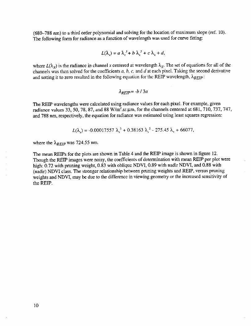
The REIP wavelengths were calculated using radiance values for each pixel. For example, given

radiance values 33, 50, 78, 87, and 88 W/m2.sr._m, for the channels centered at 681,710, 737, 747,

and 788 nm, respectively, the equation for radiance was estimated using least squares regression:

L(k,) = -0.00017557 _x3 + 0.38163 _.2 _ 275.45 _._ + 66077,

where the _,REIP was 724.55 nm.

The mean REIPs for the plots are shown in Table 4 and the REIP image is shown in figure 12.

Though the REIP images were noisy, the coefficients of determination with mean REIP per plot were

high: 0.72 with pruning weight, 0.83 with oblique NDVI, 0.89 with nadir NDVI, and 0.88 with

(nadir) NDVI class. The stronger relationship between pruning weights and REIP, versus pruning

weights and NDVI, may be due to the difference in viewing geometry or the increased sensitivity of

the REIP.

10

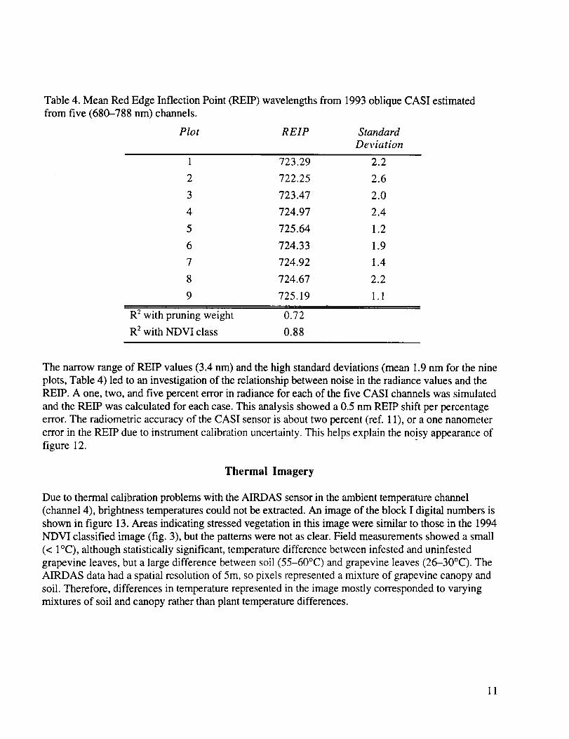
Table4. MeanRedEdgeInflectionPoint(REIP)wavelengthsfrom 1993obliqueCASI estimatedfrom five (680-788nm) channels.

Plot REIP Standard

Deviation

1 723.29 2.2

2 722.25 2.6

3 723.47 2.O

4 724.97 2.4

5 725.64 1.2

6 724.33 1.9

7 724.92 1.4

8 724.67 2.2

9 725.19 1.1

R 2 with pruning weight

R 2 with NDVI class

0.72

0.88

The narrow range of REIP values (3.4 nm) and the high standard deviations (mean 1.9 nm for the nine

plots, Table 4) led to an investigation of the relationship between noise in the radiance values and the

REIP. A one, two, and five percent error in radiance for each of the five CASI channels was simulated

and the REIP was calculated for each case. This analysis showed a 0.5 nm REIP shift per percentage

error. The radiometric accuracy of the CASI sensor is about two percent (ref. 11), or a one nanometer

error in the REIP due to instrument calibration uncertainty. This helps explain the noisy appearance of

figure 12.

Thermal Imagery

Due to thermal calibration problems with the AIRDAS sensor in the ambient temperature channel

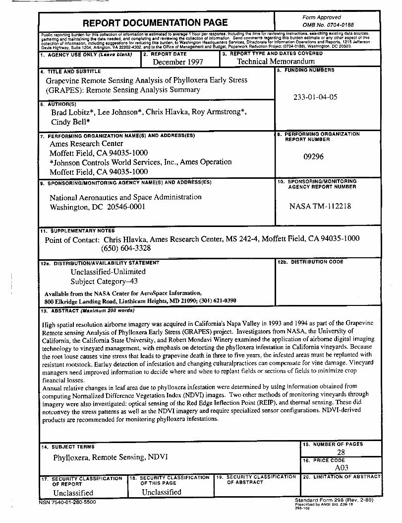
(channel 4), brightness temperatures could not be extracted. An image of the block I digital numbers is

shown in figure 13. Areas indicating stressed vegetation in this image were similar to those in the 1994

NDVI classified image (fig. 3), but the patterns were not as clear. Field measurements showed a small

(< 1°C), although statistically significant, temperature difference between infested and uninfested

grapevine leaves, but a large difference between soil (55-60°C) and grapevine leaves (26-30°C). The

AIRDAS data had a spatial resolution of 5m, so pixels represented a mixture of grapevine canopy and

soil. Therefore, differences in temperature represented in the image mostly corresponded to varying

mixtures of soil and canopy rather than plant temperature differences.

11

CONCLUSIONS

To determine phylloxera infestation and predict future vine stress using remotely sensed data, a

cooperative technology testing and development project involving a number of participants was

initiated. During this project, various digital imaging systems were flown over test sites in Napa,

California to determine the most efficient method and data available to locate and predict phylloxera

vine stress. In the course of the GRAPES project a number of different sensors were flown. Because

grapevines are a row crop, pixel sizes smaller than the row spacing can obscure the spectral

differences and make block patterns difficult to interpret. Considering the image analysis performed,

entire vineyards can be processed and patterns within blocks observed with a spatial resolution of

about three to five meters. This project acquired imagery collected over an entire vineyard, but focused

on one block or several blocks to verify the results. The smallest vineyard-unit managers consider for

many decisions is the block (about 1-10 ha), so within block variability is superfluous. Because the

cost of acquisition and processing remotely sensed digital imagery is inversely proportional to the pixel

size, three to five meters is a good tradeoff between cost and spatial resolution.

The use of the same sensor for each flight, while not necessary, would greatly simplify data

processing and improve confidence in the derived image products. If the spatial resolution between

sensors is different, the resolution of the sensors has to be matched by image analysis techniques.

Spectral values between different systems do not have to match; as long as the data sets are not

significantly different, becaw, e clustering each NDVI image and the NDVI itself compensates for

differences in atmospheric conditions.

The mean spectral-clas,_ ,,aluc per plot was found to be highly correlated to the pruning weight per plot

for each year. The correlation between pruning weight and mean NDVI class per plot was higher than

the correlation between pruning weight and mean NDVI value per plot (R 2 = 0.76 compared to 0.66).

Good results with digitally acquired imagery were achieved without sensor calibration and atmospheric

correction by using spectrally classified data to examine relative differences in canopy cover per year.

Preliminary results indicate this classification procedure should provide improved results with scanned

photography as well as digitally acquired imagery.

Histograms of the spectrally classified, digitally acquired, images for block I also showed a change

from a homogeneous block in 1993, with a sharply peaked histogram, to a relatively flat histogram,

non-uniform block, in 1994. If an unsupervised classification procedure is used, then the classified

images can be ground truthed or compared to other imagery to determine the relationship between

classes, canopy cover, and damage level. This information can be used to determine a threshold for

classes of stressed or conspicuously damaged vegetation. The effect of different trellising types or row

spacing on NDVI was not explicitly investigated, but the approach should provide a good indication of

relative differences within a given field.

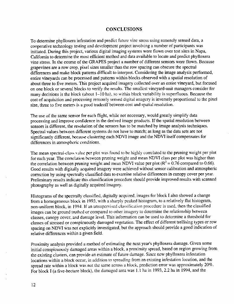
Proximity analysis provided a method of estimating the next year's phylloxera damage. Given some

initial conspicuously damaged areas within a block, a proximity spread, based on region growing from

the existing clusters, can provide an estimate of future damage. Since new phylloxera infestation

locations within a block occur, in addition to spreading from an existing infestation location, and the

spread rate within a block was not the same across a block, prediction error was approximately 20%.

For block I (a five-hectare block), the damaged area was 1.1 ha in 1993, 2.2 ha in 1994, and the

12

estimateddamagedareain 1994was1.8ha,with anerrorof aboutone-hectare.Phylloxeraarealsousuallywell establishedby thetimeadamagedareais largeenoughto beconsideredacenterofgrowth.By thefollowing yeartheblockwill bemoderatelyor heavilydamaged,andcombinedwiththe largepredictionerror,apredictionbeyondoneyearis notpractical.Spreadanalysisdoes,however,provideatool for exploringdifferentscenariosof spreadratesandgrowthcenters.Insufficienttestingwasdoneto determineif a singlegrowthratecouldbeuniformly appliedtovineyardblocksandstill obtainreasonablyaccuratepredictions,but theresultsof thisstudysuggestdifferentgrowthratesareneeded.

REIPresultsandthermalimageryfor theplotswerepromising,but lessmeaningfulthantheNDVIproducts.TheREIPresultsagreedwell with thepruningweightsandNDVI classresults,but theyrequirespecialnarrowspectralbandpassfiltersalongtherededgethatarenotcommonlyavailable.Dueto thenarrowrange(afewnanometers),REIPanalysisalsorequiresdetailedspectralandradiometriccalibrationthroughoutthe image.This isacurrentproblemwith CCD (chargecoupleddevice)arrays,andthedataneedto bestableif multi-temporalstudiesareto bepractical.Patterns,indicatingstressedvegetation,werepresentin thethermalimagery,butwerenotasdistinctasin theNDVI imagery.Leaf temperaturewasdifficult to measuredueto theopencanopy.As an indicationofcanopycoverandvegetativehealth,theeasilyderivedNDVI andfollowingclassifiedimagerywereeasierto interpretthantheREIPor thethermalimagery.

Commercialairborneimageryacquisitionservicesexistto providethedataneededfor generatingNDVI products.Only aredandanearinfraredchannelareneededto computeanNDVI, butmultiplechannelsin thered to near-infraredspectralregionareneededfor computingtheREIP.A thermalsensoris neededto acquirethermalimagery.In thenext fewyears(1998)satelliteswill providecommercialmultispectraldatawith four-meterspatialresolution.Throughproceduressuchasthoseoutlinedhere,airborneimageryacquiredin thevisibleandnear-infraredcancomplementvineyardmanagers'knowledgegainedfrom conventionalground-basedtechniques,aerialphotography,andexperience.

Theimageryindicatedplantstressdueto phylloxeraandothersources,suchaswaterstress.Airborneimagerycanservemultiplerolesin vineyardmanagement.Multi-yearimagerycanbeusedto helpidentifythetypeof stressif thegrowthpatterncanbeidentified.Thebenefitsversusthecostsofmultiple flightsperyeararestill unknown,but the informationgainedfrom asingleflight peryearwasconsideredworthwhileto theMondavivineyardmanagementteam.Knowledgeof thepatternchangefrom year-to-yearallowsthevineyardmanagerto interveneandapplyremedialmeasuresaswell asprovidedatafor financialforecasts.

RECOMMENDATIONS

To monitor the phylloxera infestation of a vineyard, digital multispectral imagery should be acquired at

least once a year at full canopy, between mid-season and harvest. The imagery should have a spatial

resolution not to exceed three meters and the use of the same sensor package for each data collection

period is important. The data can be used to generate co-registered, classified, NDVI data sets for

multi-year comparisons. In classifying one block, five or six spectral classes are sufficient, but ten to

twelve should be used for an image of an entire vineyard. A small number of classes makes image

product interpretation easier, but some features could be missed with too few classes. To avoid

13

problemswith changingamountof bare soil in the imagery, a threshold should be used to eliminate

low NDVI pixels.

COMPUTER FACILITIES

All image processing described above was performed at the NASA Ames Research Center ECOSAT

Computational Facility with ERDAS Imagine 8.20 (ERDAS, Inc., Atlanta, GA) running under Solaris

on a Sun Microsystems SPARCstation. The processing described here used standard image

processing routines available on a PC, using any one of number of commonly available geographic

image processing software packages. More information about satellite image processing, much of

which also applies to aircraft imagery, including software sources, can be found in the Satellite

Imagery Frequently Asked Questions (FAQ) at

http://www.geog.nottingham.ac.uk/remote/satfaq.html.

ACKNOWLEDGMENTS

Work to establish the plot size and locations and phylloxera levels within the plots was performed by

E. Weber (University of California Cooperative Extension Napa County), J. De Benedictis (UC

Davis), R. Baldy, and M. Baldy (both Califomia State University Chico). GPS data were collected by

C. Bell (Johnson Controls World Services, NASA Ames Research Center, currently California

Department of Forestry through UC Davis) and B. Osbom (UC Davis, currently Glen Ellen Cameros

Winery). Pruning weights were courtesy of Robert Mondavi Winery (D. Bosch). A. B1edsoe, D.

Bosch (both Robert Mondavi Winery), and P. Freese (Wine Grow) provided guidance throughout the

project. Other contributors included D. Peterson, J. Salute, and V. Vanderbilt (all NASA Ames

Research Center). The work described in this paper was performed at the NASA Ames Research

Center under UPN 233-01-04-05 in fiscal years 1993-1995.

PROJECT URL (WEB PAGE ADDRESS)

http://geo.arc.nasa.gov/sge/grapes/grapes.htrnl

14

APPENDIX: SENSOR SPECIFICATIONS

The sensors flown in the course of this project were summarized in Table 1, but this appendix

describes these sensors in more detail. The sensors were flown on aircraft platforms at low, medium,

and high altitudes and had various spectral characteristics. Half of these were charge-coupled device

(CCD) sensors and the other half were scanners. Scanning sensors use a linear array of photo

detectors that measures the intensity of radiance within some wavelength region as the sensor passes

(or sweeps) over the landscape, while a CCD sensor uses an array of detectors and takeg a "snapshot"

of the landscape.

Sensors measure radiant intensity at some wavelength range and have two types of resolution: spatial

and radiometric. The wavelength region of each sensor channel is determined by the spectral response

function of the wavelength filter, and the bandwidth of the filter at half maximum value is the full

width half maximum (P'WHM). Spatial resolution was defined on page 3 as related to aircraft altitude,

but this was just another way of describing a detector's instantaneous field of view (IFOV), or angular

width. Because a detector's IFOV is fixed, a change in altitude changes the amount of landscape

subtended by the detector. This quantity is expressed in radians, where 1.0 r = n/180 °, or usually in

milliradians. The radiometric resolution of these sensors was eight bits, except the CASI sensor with

twelve bits and the AIRDAS sensor with sixteen bits. Some of these sensors, like CASI, can be

reconfigured for multiple purposes, but Table A 1 describes the configurations used with the GRAPES

project.

15

Sensor

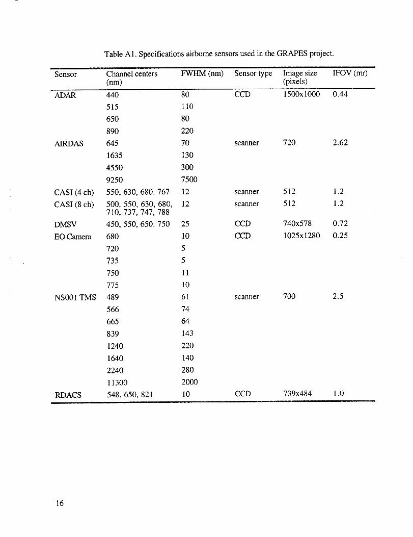
TableA 1.Specificationsairbornesensorsusedin theGRAPESproject.

i

Channel centers FWHM (nm) Sensor type Image size(nm) (pixels)

rFOV(mr)

ADAR

AIRDAS

CASI (4 ch)

CASI (8 ch)

DMSV

EO Camera

NS001 TMS

RDACS

440 80 CCD 1500x1000

515 110

650 80

890 220

645 70 scanner 720

1635 130

4550 300

9250 7500

550, 630, 680, 767 12 scanner 512

500, 550, 630, 680, 12 scanner 512710, 737, 747, 788

450,550, 650,750 25 CCD 740x578

680 10 CCD 1025x1280

720 5

735 5

750 11

775 10

489 61 scanner 700

566 74

665 64

839 143

1240 220

1640 140

2240 280

11300 2000

548,650, 821 10 CCD 739x484

0.44

2.62

1.2

1.2

0.72

0.25

2.5

1.0

16

REFERENCES

1. Granett, J., A. Goheen, and L. Lider. 1987. Grape phylloxera in California. California Agriculture

41(1):10-12.

2. Granett, J., J. De Benedictis, J. Wolpert, E. Weber, and A. Goheen. 1991. Deadly insect pest

poses increased risk to north coast vineyards. California Agriculture 45(2):30-32.

3. Wildman, W. E., R. T. Nagaoka, and L. A. Lider. 1983. Monitoring spread of grape phylloxera

by color infrared aerial photography and ground investigation. American Journal of Enology

and Viticulture 34(2):83-94.

4. Johnson, L. F., B. Lobitz, R. Armstrong, R. Baldy, E. Weber, J. De Benedictis, and D. Bosch.

1996. Airborne imaging aids vineyard canopy evaluation. California Agriculture 50(4): 14-18.

5. Ambrosia, V. G., J. A. Brass, J. B. Allen, E. A. Hildum, and R. G. Higgins. 1994. AIRDAS,

development of a unique four channel scanner for natural disaster assessment. First

International Airborne Remote Sensing Conference and Exhibition, Strasbourg, France, 11-15

September 1994.

6. Borstad Associates, Ltd. 1991. Low cost digital remote sensing using the Compact Airborne

Spectrographic Imagery. Sidney, British Columbia, Canada: Borstad Associates, Ltd.

7. Lyon, R. J. P. 1994. SpecTerra digital multi-spectral video image data formats. Stanford, CA:

SpecTerra Systems, Pty, Ltd.

8. Tucker, C. J. 1979. Red and photographic infrared linear combinations for monitoring vegetation.

Remote Sensing of Environment 8:127-150.

9. Duda R. and P. Hart. 1973. Pattern Classification and Scene Analysis. New York: John Wiley and

Sons, Inc.

10. Baret, F., S. Jacquemoud, G. Guyot, and C. Leprieur. 1992. Modeled analysis of the biophysical

nature of spectral shifts and comparison with information content of broad bands. Remote

Sensing of Environment 41:133-142.

11. Babey, S. and R. Softer. 1992. Radiometric calibration of the compact airborne spectrographic

imager (CASI). Canadian Journal of Remote Sensing 18(4):233-242.

17

6O

0 • _ m

40 ......

30 Healthy Leaf

20 -- Stressed Leaf

....... Soil10

0 I - i I I I I I ' I I

400 500 600 700 800 900 1000 1100 1200 1300

Wavelength (nm)

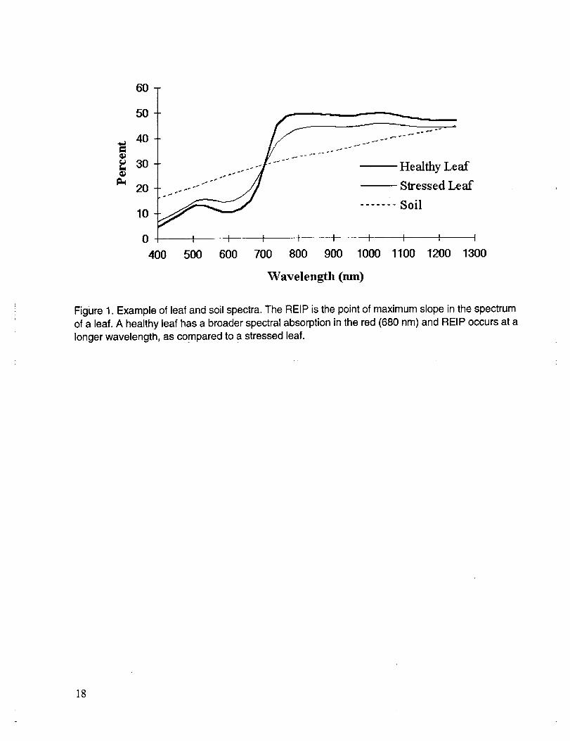
Figure 1. Example of leaf and soil spectra. The REIP is the point of maximum slope in the spectrum

of a leaf. A healthy leaf has a broader spectral absorption in the red (680 nm) and REIP occurs at a

longer wavelength, as compared to a stressed leaf.

18

1994 red channel

1993 red 5x5 1993 red 7x7 1993 red 9x9

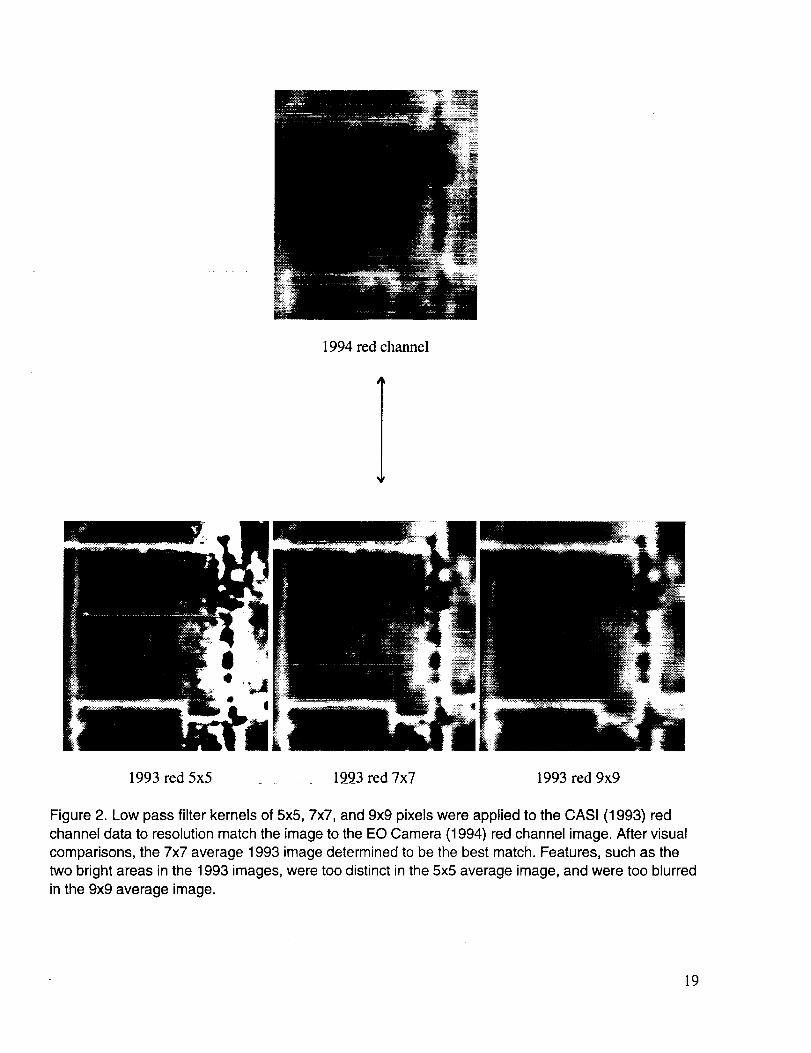
Figure 2. Low pass filter kernels of 5x5, 7x7, and 9x9 pixels were applied to the CASI (1993) red

channel data to resolution match the image to the EO Camera (1994) red channel image. After visual

comparisons, the 7x7 average 1993 image determined to be the best match. Features, such as the

two bright areas in the 1993 images, were too distinctin the 5x5 average image, and were too blurred

in the 9x9 average image.

19

1993 1994

Figure 3. Block I classified NDV11993 and 1994 images, where the lowest NDVI values are shown in

black and the highest values in white. Also shown in white are the boundaries of the block and plots

within the block. A large patch of low canopy cover vines can be seen in the lower right, contrastingwith the trees at the extreme right edge of the 1993 image. Multiple patches of low canopy cover

vines can be seen in the 1994 image. "Rainbow" colored images were used during image analysis

and initial products were colored by vigor level: brown for little or no vegetation, yellow for some -

vegetation, and green for high vegetation cover.

45

40

35

30

252O

15

10

5

0

0 1 2 3 4 5 6 7 8 9 10

Class

Figure 4. NDVI class histograms for block I. Class 0 percentages represent pixels below the bare soil

threshold. Only ten of the twelve classes used for the ranch were present in block I.

2O

JZ

10

8

6

4

2

0

0

[]

[]

[]

[]

[]

• 93

[] 94

r-im

_) I I I I

1 2 3 4 5

Pruning Weight (kg)

Figure 5. Block I pruning weight per plot for both 1993 and 1994 correlated well with the per-plotmean Normalized Difference Vegetation Index class number. In 1993, R2 = 0.60; in 1994, R2 = 0.88;and for both combined R2 = 0.76.

Figure 6. NDVI class difference image for 1993 and 1994. This image represents canopy coverchange. Areas with the largest class value decrease are white and those areas with a class value

increase are black. The medium-gray area in the lower right exhibited no change, also shown in whiteare the boundaries of the block and the plots within the blockl

21

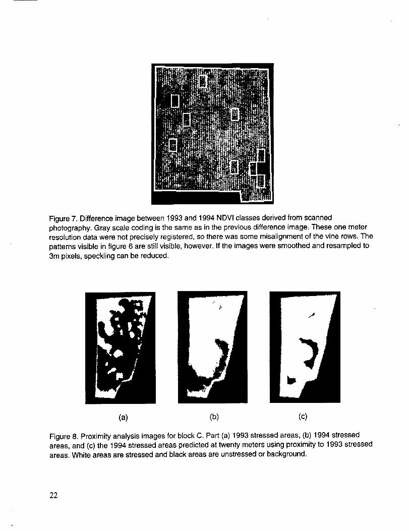
Figure 7. Difference image between 1993 and 1994 NDVI classes derived from scanned

photography. Gray scale coding is the same as in the previous difference image. These one meterresolution data were not precisely registered, so there was some misalignment of the vine rows. The

patterns visible in figure 6 are still visible, however. If the images were smoothed and resampled to

3m pixels, speckling can be reduced.

(a) (b) (c)

Figure 8. Proximity analysis images for block C. Part (a) 1993 stressed areas, (b) 1994 stressedareas, and (c) the 1994 stressed areas predicted at twenty meters using proximity to 1993 stressed

areas. White areas are stressed and black areas are unstressed or background.

22

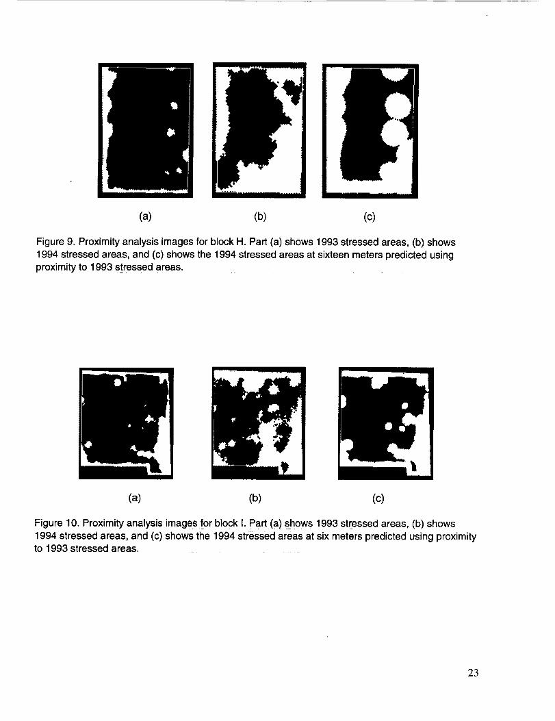
(a) (b) (c)

Figure9. Proximityanalysisimagesfor blockH. Part(a)shows1993stressedareas,(b)shows1994stressedareas,and(c) showsthe 1994stressedareasat sixteenmeterspredictedusingproximityto 1993stressedareas.

(a) (b) (c)

Figure10.Proximityanalysisimagesfor blockI. Part(a)showsi993 stressedareas,(b)shows1994stressedareas,and (c)showsthe 1994stressedareasat six meterspredictedusingproximityto 1993stressedareas.

23

(a) (b) (c)

Figure 11. Proximity analysis images for block J. Part (a) shows 1993 stressed areas, (b) shows1994 stressed areas, and (c) shows the 1994 stressed areas at six meters predicted using proximity

to 1993 stressed areas.

i i

Figure 12. REIP image of block I. The REIP was computed using five channels as input to a third

order polynomial. Some distortion of the image is apparent due to aircraft roll, but the boundary of theblock is visible and the dark areas (shorter REIP) correspond to stressed areas from the 1993

classified NDVI image (fig. 3).

24

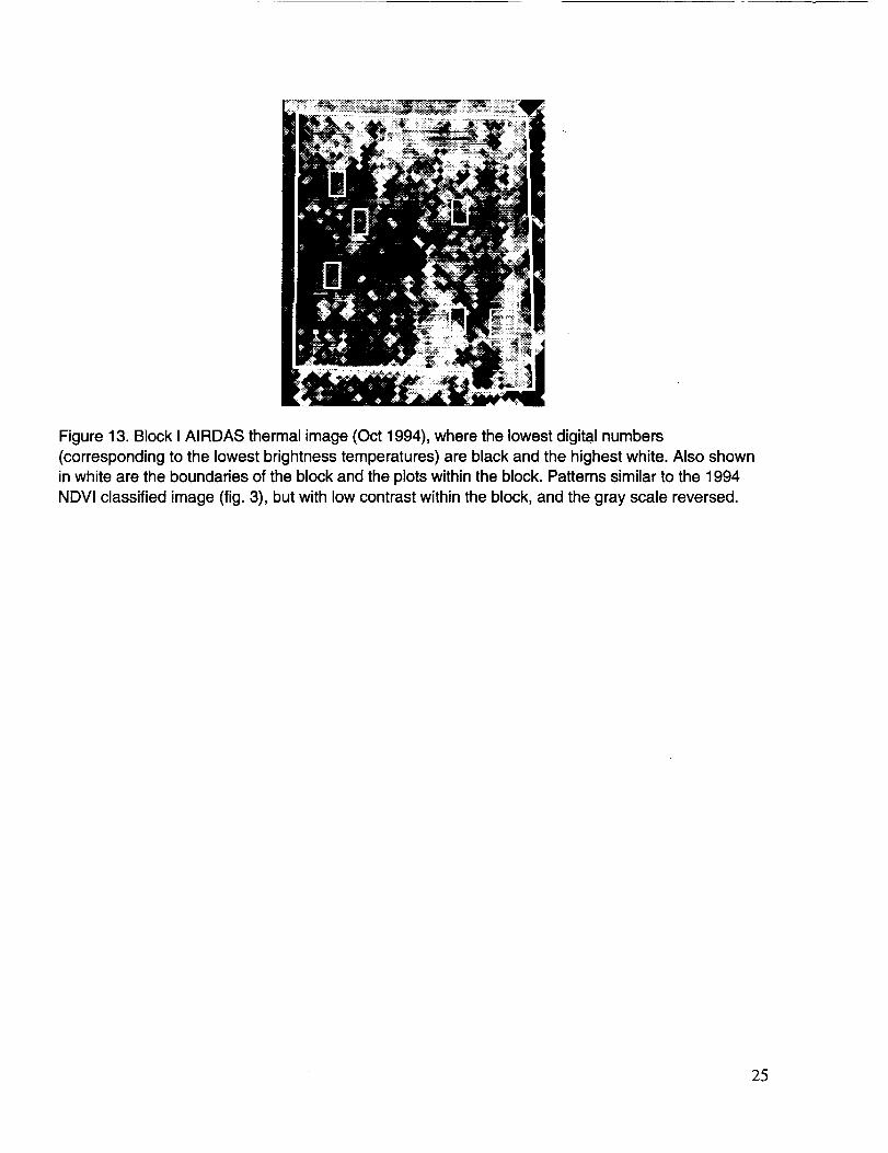
Figure13.BlockI AIRDASthermalimage(Oct1994),wherethelowestdigitalnumbers(correspondingto the lowestbrightnesstemperatures)areblackandthe highestwhite.Alsoshowninwhiteare the boundariesofthe blockandthe plotswithinthe block.Patternssimilarto the 1994NDVIclassifiedimage(fig.3), butwith lowcontrastwithintheblock,andthegrayscalereversed.

25

Form ApprovedREPORT DOCUMENTATION PAGE oM8No.0704-0188

Public reporting burden for this collection of information is estimated to average 1 hour per response, including the time for reviewing instructions, searching existing data sources,

gathering and maintaining the data needed, and completing and reviewing the collection of information. Send comments regarding this burden estimate or any other aspect of this

collection of Information. includ ng suggestions for reducing this burden, to Washington Headquarters Services, Directorate for information Operations and Repods, 1215 Jefferson

Davis Highway, Suite 1204, Arlington, VA 22202-4302, and to the Office of Management and Budget, Paperwork Reduction Pro iect (0704-0188), Wash ngton, DC 20503.

1. AGENCY USE ONLY (Leave blank) 2. REPORT DATE 3. REPORT TYPE AND DATES COVERED

December 1997 Technical Memorandum

4. TITLE AND SUBTITLE

Grapevine Remote Sensing Analysis of Phylloxera Early Stress

(GRAPES): Remote Sensing Analysis Summary

6. AUTHOR(S)

Brad Lobitz*, Lee Johnson*, Chris Hlavka, Roy Armstrong*,

Cindy Bell*

7. PERFORMING ORGANIZATION NAMEtS) AND ADDRESS(ES)

Ames Research Center

Moffett Field, CA 94035-1000

*Johnson Controls World Services, Inc., Ames Operation

Moffett Field, CA 94035-1000

9. SPONSORING/MONITORING AGENCY NAME(S) AND ADDRESS(ES)

National Aeronautics and Space Administration

Washington, DC 20546-0001

11. SUPPLEMENTARYNOTES

Point of Contact:

5. FUNDING NUMBERS

, lid

233-01-04-05

8. PERFORMING ORGANIZATIONREPORT NUMBER

09296

10. SPONSORING/MONITORINGAGENCY REPORT NUMBER

NASA TM-112218

Chris Hlavka, Ames Research Center, MS 242-4, Moffett Field, CA 94035-1000

(650) 604-3328

12b. DISTRIBUTION CODE12a. DISTRIBUTION/AVAILABILITY STATEMENT

Unclassified-Unlimited

Subject Category--43

Available from the NASA Center for AeroSpace Information,

800 Elkridge Landing Road, Linthicum Heights, MD 21090; (301) 621-0390II1[

13. ABSTRACT (Maximum 200 words)

High spatial resolution airborne imagery was acquired in California's Napa Valley in 1993 and 1994 as part of the Grapevine

Remote sensing Analysis of Phylloxera Early Stress (GRAPES) project. Investigators from NASA, the University of

California, the California State University, and Robert Mondavi Winery examined the application of airborne digital imaging

technology to vineyard management, with emphasis on detecting the phylloxera infestation in California vineyards. Because

the root louse causes vine stress that leads to grapevine death in three to five years, the infested areas must be replanted with

resistant rootstock. Earluy detection of infestation and changing cuhuralpractices can compensate for vine damage. Vineyard

managers need improved information to decide where and when to replant fields or sections of fields to minimize crop

financial losses.

Annual relative changes in leaf area due to phylloxera infestation were determined by using information obtained from

computing Normalized Difference Vegetation Index (NDVI) images. Two other methods of monitoring vineyards through

imagery were also investigated: optical sensing of the Red Edge Inflection Point (REIP), and thermal sensing. These did

notconvey the stress patterns as well as the NDVI imagery and require specialized sensor configurations. NDVI-derived

products are recommended for monitoring phylloxera infestations.

14. SUBJECTTERMS

Phylloxera, Remote Sensing, NDVI

17. SECURITY CLASSIFICATION 18. SECURITY CLASSIFICATIONOF REPORT OF THIS PAGE

Unclassified Unclassified

NSN 7540-01-280-5500

19. SECURITY CLASSIFICATIONOF ABSTRACT

15. NUMBER OF PAGES

2816. PRICE CODE

A0320. LIMITATION OF ABSTRACT

Standard Form 298 (Rev. 2-89)Prescribed by ANSI Srd Z39-18298 - 102