FROM DISCRETE PARTICLES TO CONTINUUM FIELDS NEAR A

BOUNDARYABHISHEK KULKARNI

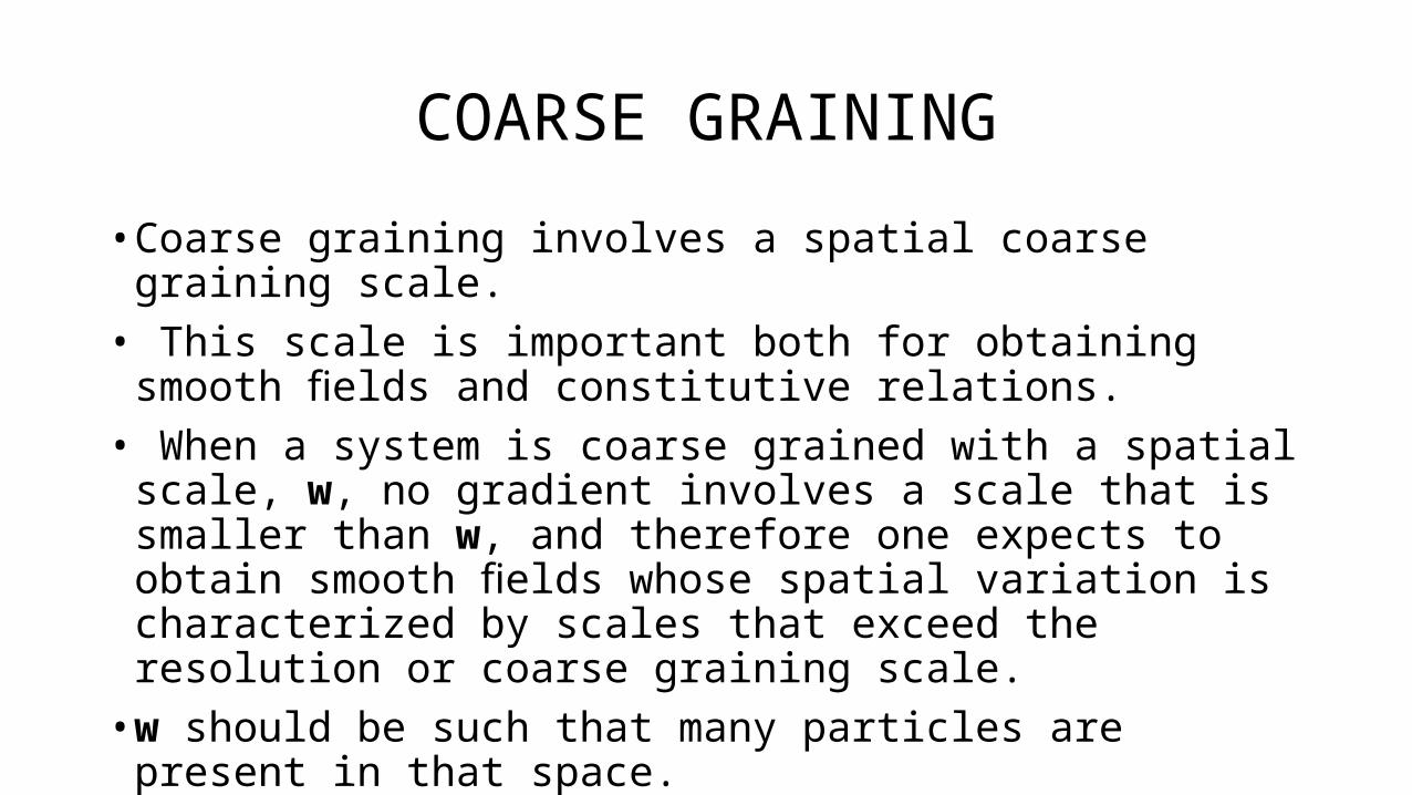
COARSE GRAINING• Coarse graining involves a spatial coarse graining scale.• This scale is important both for obtaining smooth fields and

constitutive relations.• When a system is coarse grained with a spatial scale, w, no gradient

involves a scale that is smaller than w, and therefore one expects to obtain smooth fields whose spatial variation is characterized by scales that exceed the resolution or coarse graining scale.• w should be such that many particles are present in that space.

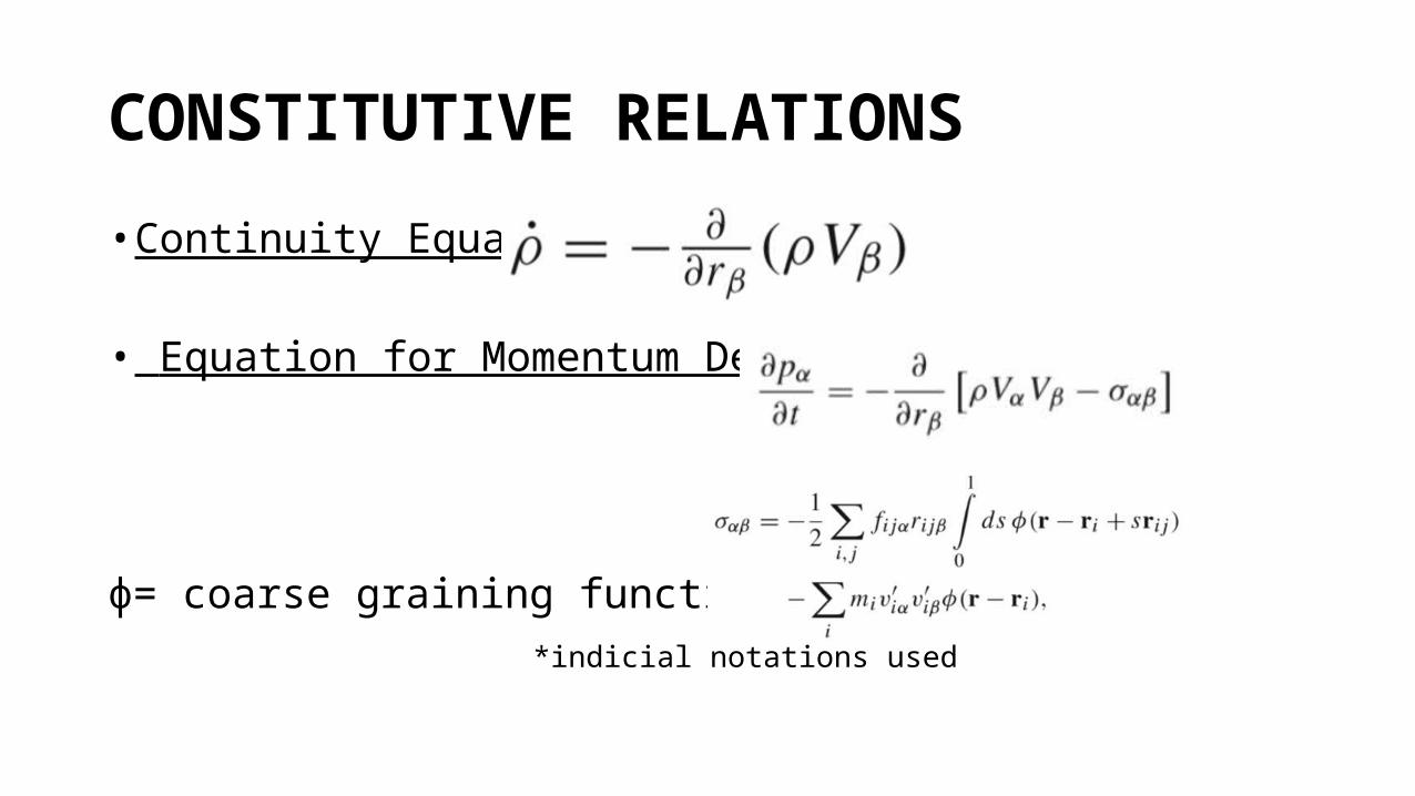
CONSTITUTIVE RELATIONS• Continuity Equation:

• Equation for Momentum Density:

ɸ= coarse graining function *indicial notations used

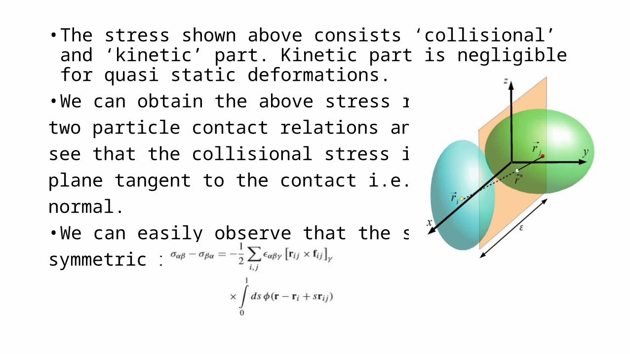
• The stress shown above consists ‘collisional’ and ‘kinetic’ part. Kinetic part is negligible for quasi static deformations.• We can obtain the above stress relation using two particle contact relations and thus we can see that the collisional stress is normal to the plane tangent to the contact i.e. stresses are normal.• We can easily observe that the stress is anti-symmetric i.e.

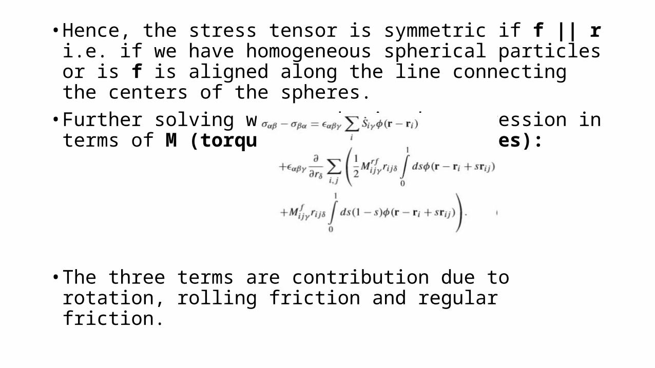
• Hence, the stress tensor is symmetric if f || r i.e. if we have homogeneous spherical particles or is f is aligned along the line connecting the centers of the spheres.• Further solving we can obtain the expression in terms of M (torque

between the particles):

• The three terms are contribution due to rotation, rolling friction and regular friction.

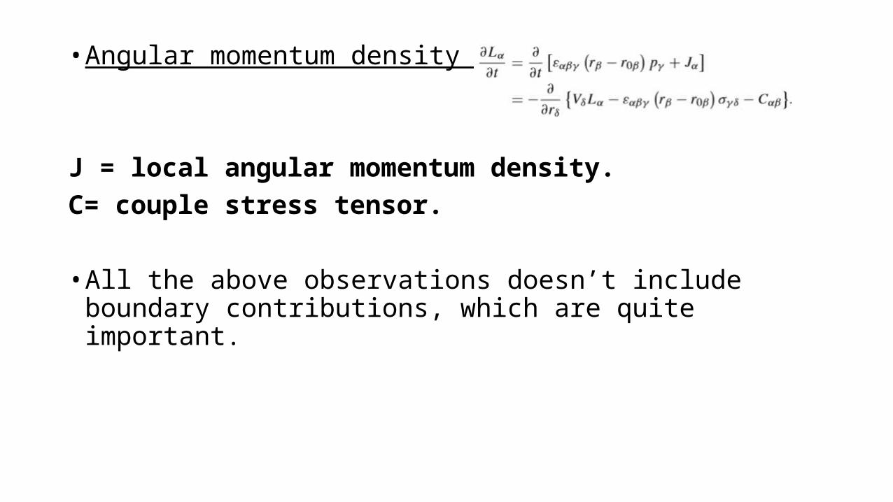
• Angular momentum density field:

J = local angular momentum density.C= couple stress tensor.

• All the above observations doesn’t include boundary contributions, which are quite important.

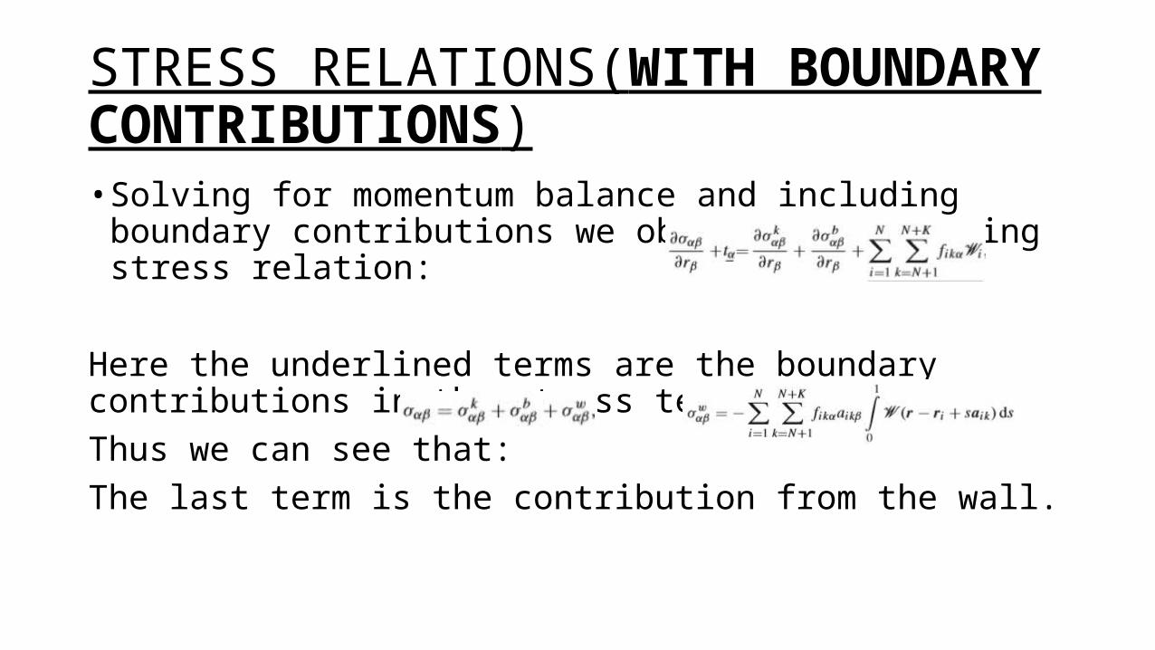
STRESS RELATIONS(WITH BOUNDARY CONTRIBUTIONS)• Solving for momentum balance and including boundary contributions

we obtain the following stress relation:

Here the underlined terms are the boundary contributions in the stress tensor.Thus we can see that: The last term is the contribution from the wall.

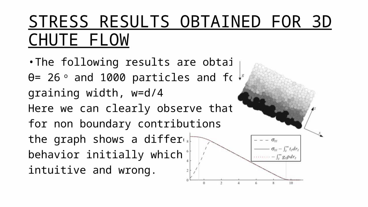
STRESS RESULTS OBTAINED FOR 3D CHUTE FLOW• The following results are obtained for Ɵ= 26 o and 1000 particles and for coarsegraining width, w=d/4 Here we can clearly observe that for non boundary contributionsthe graph shows a different behavior initially which is not intuitive and wrong.

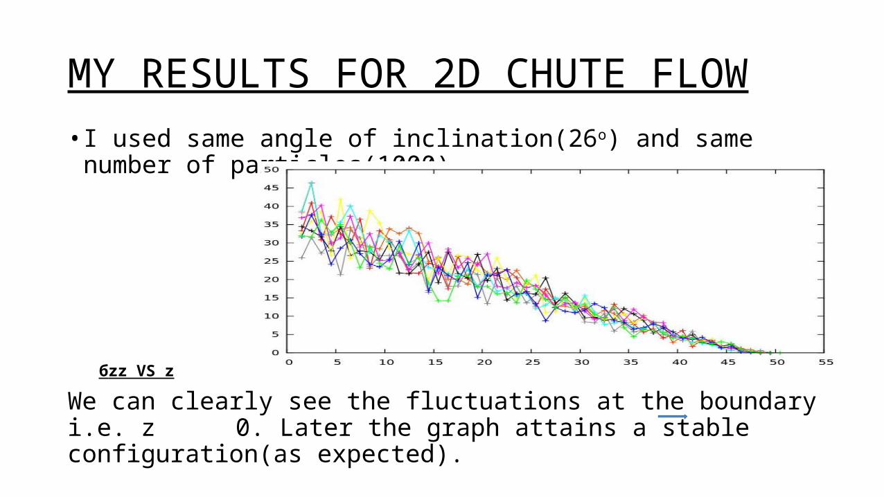
MY RESULTS FOR 2D CHUTE FLOW• I used same angle of inclination(26o) and same number of

particles(1000).

бzz VS z

We can clearly see the fluctuations at the boundary i.e. z 0. Later the graph attains a stable configuration(as expected).

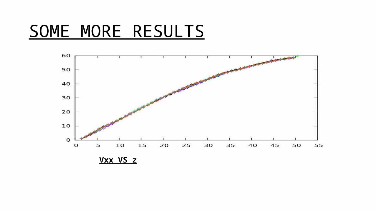
SOME MORE RESULTS

Vxx VS z

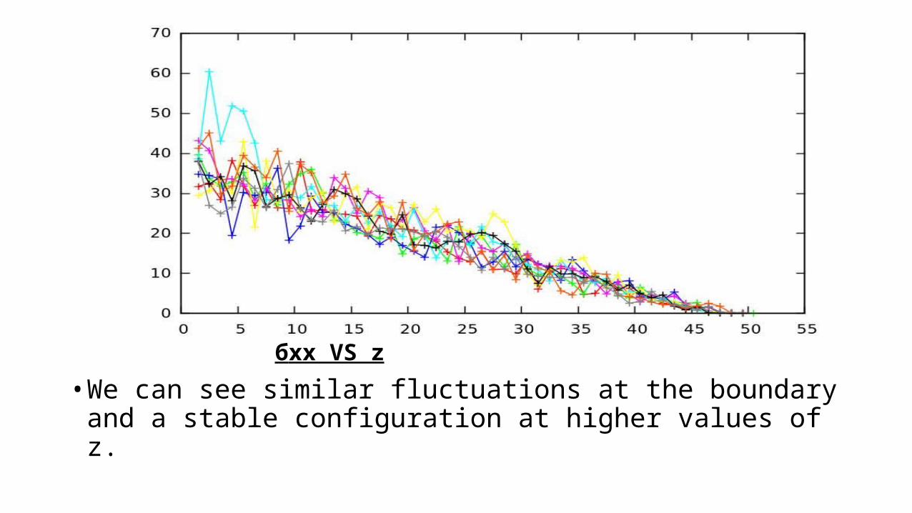
бxx VS z

• We can see similar fluctuations at the boundary and a stable configuration at higher values of z.

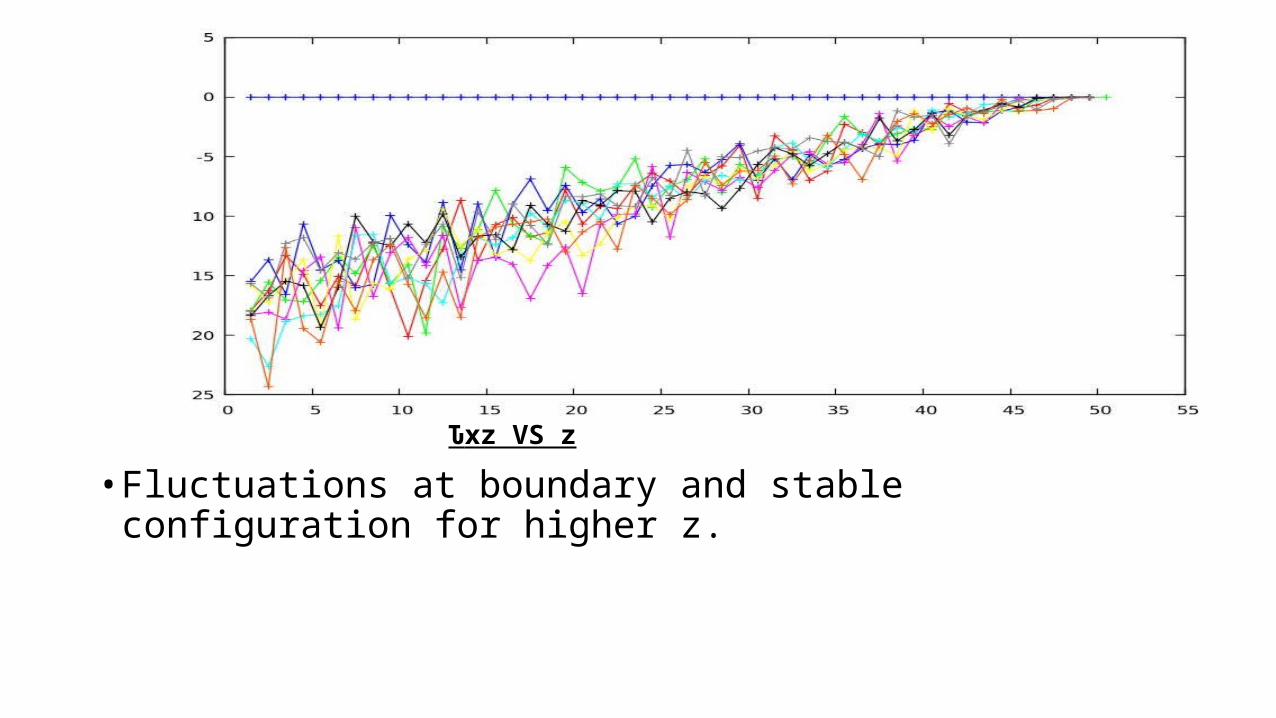
Ԏxz VS z

• Fluctuations at boundary and stable configuration for higher z.

THANK YOU