Embed Size (px)
Citation preview
Gram–Schmidt Orthogonalization:100 Years and More
Ake Bjorck
IWMS, June 5–8, 2010, Shanghai
Definition
Gram–Schmidt Process:
The process of forming an orthogonal sequence {yk} from alinearly independent sequence {xk} of members of aninner-product space.
James and James, Mathematical Dictionary, 1949
This process and the related QR factorization is a fundamentaltool of numerical linear algebra.
The earliest linkage of the names Gram and Schmidt todescribe this process appears to be in a paper by Y. K. Wong,An application of orthogonalization process to the theory ofleast squares. Ann. Math. Statist., 6, 53-75, 1935.

Outline
Early History
Classical versus Modified Gram–Schmidt
Loss of Orthogonality
Least Squares Problems
The Householder Connection
Krylov Subspace Methods
Early History
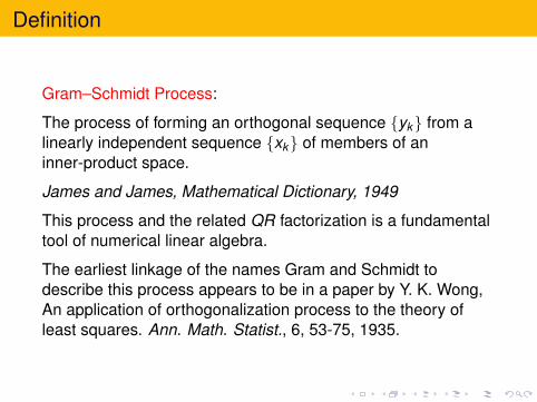
In 1907 Erhard Schmidt published an orthogonalizationalgorithm which become popular and widely used.Given n linearly independent elements a1,a2, . . . ,an in aninner-product space. The algorithm computes an orthonormalbasis q1,q2, . . . ,qn, such that
ak = r1kq1 + r2kq2 + · · ·+ rkkqk , k = 1 : n.
The matrix interpretation is that A = (a1,a2, . . . ,an) is factoredinto a product
A = (q1,q2, . . . ,qn)
r11 r12 · · · r1n
r22 · · · r2n. . .
...rnn
≡ QR.
R is upper triangular with positive diagonal entries. Thisfactorization is uniquely determined.

Early History
Schmidt used what is now known as the classicalGram–Schmidt process.
Erhard Schmidt (1876–1959), studied inGottingen under Hilbert. In 1917 heassumed a position at the University ofBerlin, where he started the famousInstitute of Applied Mathematics.
Zur Theorie der linearen und nichtlinearen Integralgleichungen.I. Teil: Entwicklung willkurlicher Funktionen nach Systemenvorgeschriebener. Math. Ann. 1907.
Early History
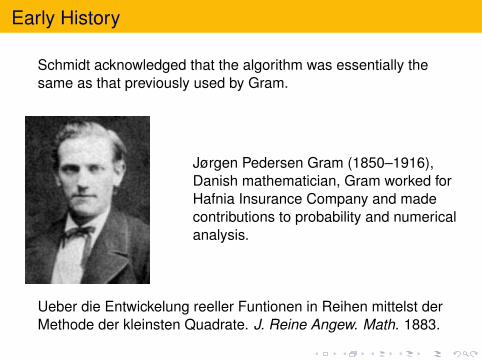
Schmidt acknowledged that the algorithm was essentially thesame as that previously used by Gram.
Jørgen Pedersen Gram (1850–1916),Danish mathematician, Gram worked forHafnia Insurance Company and madecontributions to probability and numericalanalysis.
Ueber die Entwickelung reeller Funtionen in Reihen mittelst derMethode der kleinsten Quadrate. J. Reine Angew. Math. 1883.
The Treatise of Laplace
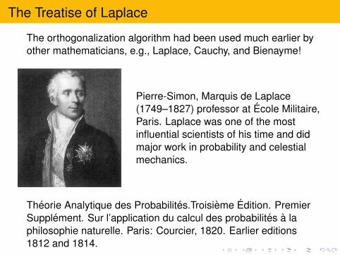
The orthogonalization algorithm had been used much earlier byother mathematicians, e.g., Laplace, Cauchy, and Bienayme!
Pierre-Simon, Marquis de Laplace(1749–1827) professor at Ecole Militaire,Paris. Laplace was one of the mostinfluential scientists of his time and didmajor work in probability and celestialmechanics.
Theorie Analytique des Probabilites.Troisieme Edition. PremierSupplement. Sur l’application du calcul des probabilites a laphilosophie naturelle. Paris: Courcier, 1820. Earlier editions1812 and 1814.
The Treatise of Laplace
Let A be an m × n matrix (m ≥ n) with linearly independentcolumns and b an m-vector of observations with normallydistributed random errors. Laplace’s treats the statistical theoryof errors in linear least squares problems
minx‖Ax − b‖2.
The particular problem he wants to solve is to estimate themass of Jupiter and Saturn from astronomical data of 6 planets
The method which Laplace introduces consists in successivelyprojecting the system of equations orthogonally to a column ofthe matrix A. Ultimately he is left with the residual vector.
The Treatise of Laplace
This is precisely the main idea behind the Gram–Schmidtprocess. However, Laplace uses what is now known as themodified Gram–Schmidt process.
Laplace used this to prove that the solution is uncorrelated withthe residual vector. For the numerical solution of his problem hesolved the corresponding 6× 6 normal equations.
A translation and modern interpretation of Laplace treatise byJulien Langou is publsihed in Technical Report CCM 280, UCDenver, Denver, Colorado, 2009
Outline
Early History
Classical versus Modified Gram–Schmidt
Loss of Orthogonality
Least Squares Problems
The Householder Connection
Krylov Subspace Methods
Classical versus Modified Gram–Schmidt
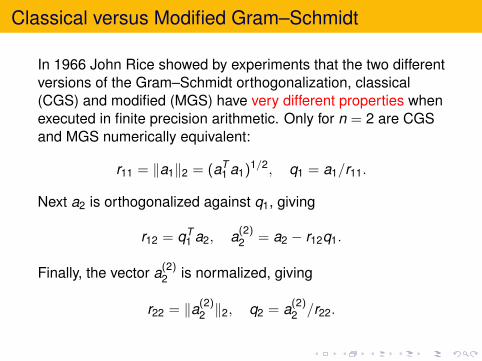
In 1966 John Rice showed by experiments that the two differentversions of the Gram–Schmidt orthogonalization, classical(CGS) and modified (MGS) have very different properties whenexecuted in finite precision arithmetic. Only for n = 2 are CGSand MGS numerically equivalent:
r11 = ‖a1‖2 = (aT1 a1)1/2, q1 = a1/r11.
Next a2 is orthogonalized against q1, giving
r12 = qT1 a2, a(2)
2 = a2 − r12q1.
Finally, the vector a(2)2 is normalized, giving
r22 = ‖a(2)2 ‖2, q2 = a(2)
2 /r22.
Classical versus Modified Gram–Schmidt
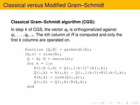
Classical Gram–Schmidt algorithm (CGS):
In step k of CGS, the vector ak is orthogonalized againstq1, . . . ,qk−1. The k th column of R is computed and only thefirst k columns are operated on.
function [Q,R] = gschmidt(A);[m,n] = size(A);Q = A; R = zeros(n);for k = 1:n
R(1:k-1,k) = Q(:,1:k-1)’*A(:,k);Q(:,k) = A(:,k) - Q(:,1:k-1)*R(1:k-1,k);R(k,k) = norm(Q(:,k));Q(:,k) = Q(:,k)/R(k,k);
end
Classical versus Modified Gram–Schmidt
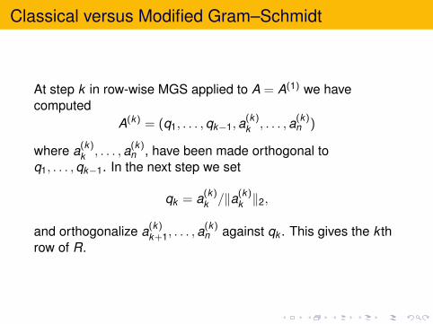
At step k in row-wise MGS applied to A = A(1) we havecomputed
A(k) = (q1, . . . ,qk−1,a(k)k , . . . ,a(k)
n )
where a(k)k , . . . ,a(k)
n , have been made orthogonal toq1, . . . ,qk−1. In the next step we set
qk = a(k)k /‖a(k)
k ‖2,
and orthogonalize a(k)k+1, . . . ,a
(k)n against qk . This gives the k th
row of R.
Classical versus Modified Gram–Schmidt
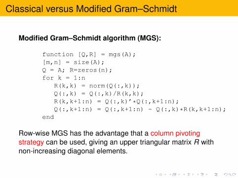
Modified Gram–Schmidt algorithm (MGS):
function [Q,R] = mgs(A);[m,n] = size(A);Q = A; R=zeros(n);for k = 1:n
R(k,k) = norm(Q(:,k));Q(:,k) = Q(:,k)/R(k,k);R(k,k+1:n) = Q(:,k)’*Q(:,k+1:n);Q(:,k+1:n) = Q(:,k+1:n) - Q(:,k)*R(k,k+1:n);
end
Row-wise MGS has the advantage that a column pivotingstrategy can be used, giving an upper triangular matrix R withnon-increasing diagonal elements.
Classical versus Modified Gram–Schmidt
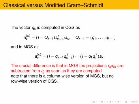
The vector qk is computed in CGS as
a(k)k = (I −Qk−1QT
k−1)ak , Qk−1 = (q1, . . . ,qk−1)
and in MGS as
a(k)k = (I − qk−1qT
k−1) · · · (I − q1qT1 )ak .
The crucial difference is that in MGS the projections rkjqk aresubtracted from aj as soon as they are computed.note that there is a column-wise version of MGS, but norow-wise version of CGS.
Outline
Early History
Classical versus Modified Gram–Schmidt
Loss of Orthogonality
Least Squares Problems
The Householder Connection
Krylov Subspace Methods
Loss of Orthogonality
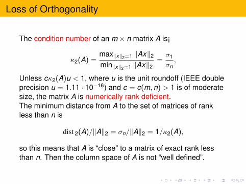
The condition number of an m × n matrix A is¡
κ2(A) =max‖x‖2=1 ‖Ax‖2min‖x‖2=1 ‖Ax‖2
=σ1
σn,
Unless cκ2(A)u < 1, where u is the unit roundoff (IEEE doubleprecision u = 1.11 · 10−16) and c = c(m,n) > 1 is of moderatesize, the matrix A is numerically rank deficient.The minimum distance from A to the set of matrices of rankless than n is
dist 2(A)/‖A‖2 = σn/‖A‖2 = 1/κ2(A),
so this means that A is “close” to a matrix of exact rank lessthan n. Then the column space of A is not “well defined”.
Loss of Orthogonality
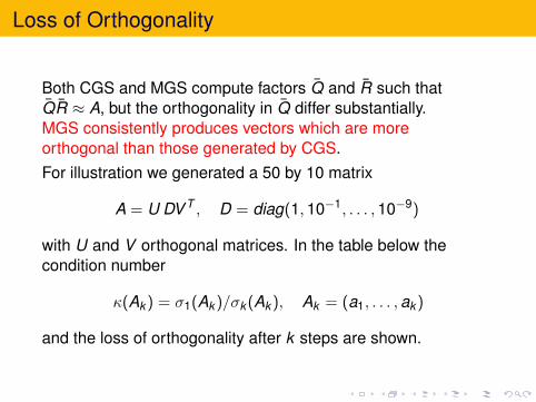
Both CGS and MGS compute factors Q and R such thatQR ≈ A, but the orthogonality in Q differ substantially.MGS consistently produces vectors which are moreorthogonal than those generated by CGS.For illustration we generated a 50 by 10 matrix
A = U DV T , D = diag(1,10−1, . . . ,10−9)
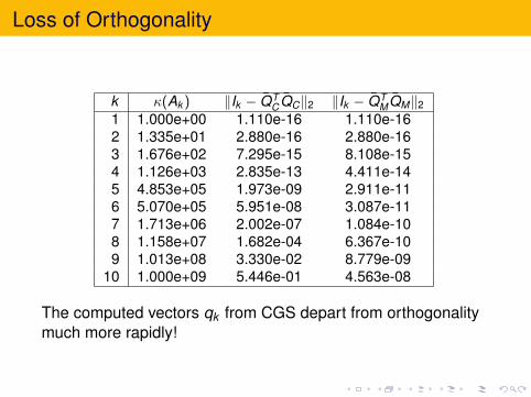
with U and V orthogonal matrices. In the table below thecondition number
κ(Ak ) = σ1(Ak )/σk (Ak ), Ak = (a1, . . . ,ak )
and the loss of orthogonality after k steps are shown.
Loss of Orthogonality
k κ(Ak ) ‖Ik − QTC QC‖2 ‖Ik − QT
MQM‖2
1 1.000e+00 1.110e-16 1.110e-162 1.335e+01 2.880e-16 2.880e-163 1.676e+02 7.295e-15 8.108e-154 1.126e+03 2.835e-13 4.411e-145 4.853e+05 1.973e-09 2.911e-116 5.070e+05 5.951e-08 3.087e-117 1.713e+06 2.002e-07 1.084e-108 1.158e+07 1.682e-04 6.367e-109 1.013e+08 3.330e-02 8.779e-09
10 1.000e+09 5.446e-01 4.563e-08
The computed vectors qk from CGS depart from orthogonalitymuch more rapidly!
Loss of Orthogonality
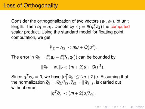
Consider the orthogonalization of two vectors (a1,a2). of unitlength. Then q1 = a1. Denote by r12 = fl(qT
1 a2) the computedscalar product. Using the standard model for floating pointcomputation, we get
|r12 − r12| < mu + O(u2).
The error in w2 = fl(a2 − fl(r12q1)) can be bounded by
‖w2 − w2‖2 < (m + 2)u + O(u2).
Since qT1 w2 = 0, we have |qT
1 w2| . (m + 2)u. Assuming thatthe normalization q2 = w2/r22, r22 = ‖w2‖2, is carried outwithout error,
|qT1 q2| < (m + 2)u/r22.
Loss of Orthogonality
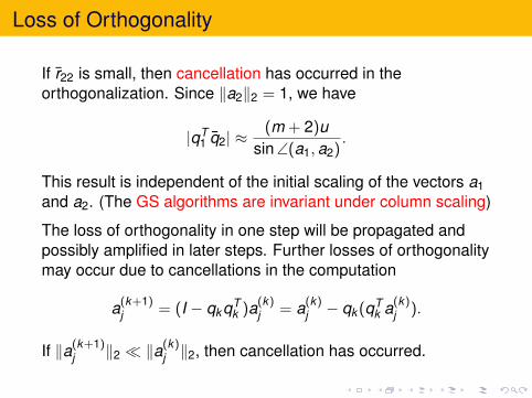
If r22 is small, then cancellation has occurred in theorthogonalization. Since ‖a2‖2 = 1, we have
|qT1 q2| ≈
(m + 2)usin ∠(a1,a2)
.
This result is independent of the initial scaling of the vectors a1and a2. (The GS algorithms are invariant under column scaling)
The loss of orthogonality in one step will be propagated andpossibly amplified in later steps. Further losses of orthogonalitymay occur due to cancellations in the computation
a(k+1)j = (I − qkqT
k )a(k)j = a(k)
j − qk (qTk a(k)
j ).
If ‖a(k+1)j ‖2 � ‖a
(k)j ‖2, then cancellation has occurred.
Loss of Orthogonality
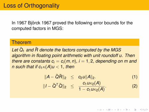
In 1967 Bjorck 1967 proved the following error bounds for thecomputed factors in MGS:
TheoremLet Q1 and R denote the factors computed by the MGSalgorithm in floating point arithmetic with unit roundoff u. Thenthere are constants ci = ci(m,n), i = 1,2, depending on m andn such that if c1κ(A)u < 1, then
‖A− QR‖2 ≤ c2u‖A‖2. (1)
‖I − QT Q‖2 ≤ c1uκ2(A)
1− c1uκ2(A). (2)
Loss of Orthogonality
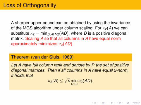
A sharper upper bound can be obtained by using the invarianceof the MGS algorithm under column scaling. For κ2(A) we cansubstitute κ2 = minD>0 κ2(AD), where D is a positive diagonalmatrix. Scaling A so that all columns in A have equal normapproximately minimizes κ2(AD)
Theorem (van der Sluis, 1969)
Let A have full column rank and denote by D the set of positivediagonal matrices. Then if all columns in A have equal 2-norm,it holds that
κ2(A) ≤√
n minD>0
κ2(AD).
Outline
Early History
Classical versus Modified Gram–Schmidt
Loss of Orthogonality
Least Squares Problems
The Householder Connection
Krylov Subspace Methods
Least Squares Problems
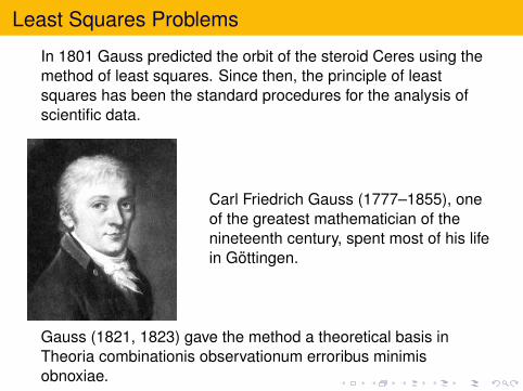
In 1801 Gauss predicted the orbit of the steroid Ceres using themethod of least squares. Since then, the principle of leastsquares has been the standard procedures for the analysis ofscientific data.
Carl Friedrich Gauss (1777–1855), oneof the greatest mathematician of thenineteenth century, spent most of his lifein Gottingen.
Gauss (1821, 1823) gave the method a theoretical basis inTheoria combinationis observationum erroribus minimisobnoxiae.
Least Squares Problems
The first publication of the method was in 1805 by A. M.Legendre in Nouvelles methodes pour la determination desorbites des cometes, Paris
Of all the principles that can be proposed, I think thereis none more general, more exact, and more easy ofapplication, than that which consists of rendering thesum of the squares of the errors a minimum.
Gauss 1809 wrote, much to the annoyance of Legendre,
Our principle, which we have made use of since 1795,has lately been published by Legendre.
Least Squares Problems
One of the most important applications of Gram–Schmidtalgorithms is for solving the linear least squares problem
minx‖Ax − b‖2,
It is assumed that the errors in b are independent and equallydistributed. The solution is characterized by r ⊥ R(A), wherer = b − Ax is the residual vector.
A related problem is the conditional least squares problem.
miny‖y − b‖22 subject to AT y = c.
A unified treatment of these two problems can be obtained asfollows:
Least Squares Problems
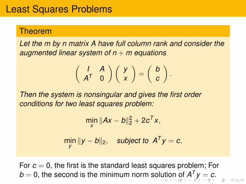
TheoremLet the m by n matrix A have full column rank and consider theaugmented linear system of n + m equations(
I AAT 0
)(yx
)=
(bc
).
Then the system is nonsingular and gives the first orderconditions for two least squares problem:
minx‖Ax − b‖22 + 2cT x ,
miny‖y − b‖2, subject to AT y = c,
For c = 0, the first is the standard least squares problem; Forb = 0, the second is the minimum norm solution of AT y = c.
Perturbation Analysis
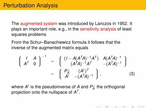
The augmented system was introduced by Lanczos in 1952. Itplays an important role, e.g., in the sensitivity analysis of leastsquares problems
From the Schur–Banachiewicz formula it follows that theinverse of the augmented matrix equals I A
AT 0
−1
=
(I − A(ATA)−1AT ) A(ATA)−1
(ATA)−1AT −(ATA)−1
=
P⊥A (A†)T
A† −(ATA)−1
, (3)
where A† is the pseudoinverse of A and P⊥A the orthogonalprojection onto the nullspace of AT .
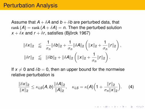
Perturbation Analysis
Assume that A + δA and b + δb are perturbed data, thatrank (A) = rank (A + δA) = n. Then the perturbed solutionx + δx and r + δr , satisfies (Bjorck 1967)
‖δx‖2 /1σn‖δb‖2 +
1σn‖δA‖2
(‖x‖2 +
1σn‖r‖2
),
‖δr‖2 / ‖δb‖2 + ‖δA‖2(‖x‖2 +
1σn‖r‖2
).
If x 6= 0 and δb = 0, then an upper bound for the normwiserelative perturbation is
‖δx‖2‖x‖2
≤ κLS(A,b)‖δA‖2‖A‖2
, κLS = κ(A)(
1 +‖r‖2σn‖x‖2
). (4)
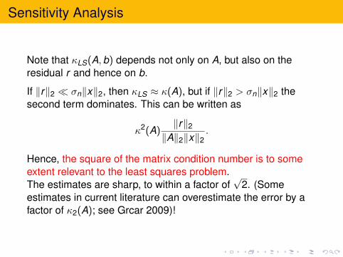
Sensitivity Analysis
Note that κLS(A,b) depends not only on A, but also on theresidual r and hence on b.
If ‖r‖2 � σn‖x‖2, then κLS ≈ κ(A), but if ‖r‖2 > σn‖x‖2 thesecond term dominates. This can be written as
κ2(A)‖r‖2
‖A‖2‖x‖2.
Hence, the square of the matrix condition number is to someextent relevant to the least squares problem.The estimates are sharp, to within a factor of
√2. (Some
estimates in current literature can overestimate the error by afactor of κ2(A); see Grcar 2009)!
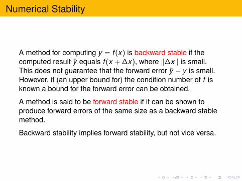
Numerical Stability
A method for computing y = f (x) is backward stable if thecomputed result y equals f (x + ∆x), where ‖∆x‖ is small.This does not guarantee that the forward error y − y is small.However, if (an upper bound for) the condition number of f isknown a bound for the forward error can be obtained.
A method is said to be forward stable if it can be shown toproduce forward errors of the same size as a backward stablemethod.
Backward stability implies forward stability, but not vice versa.
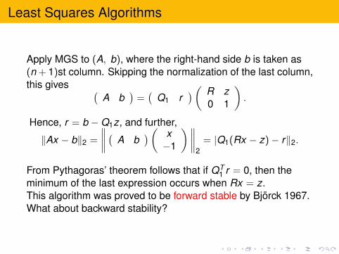
Least Squares Algorithms
Apply MGS to (A, b), where the right-hand side b is taken as(n + 1)st column. Skipping the normalization of the last column,this gives (
A b)
=(
Q1 r)( R z
0 1
).
Hence, r = b −Q1z, and further,
‖Ax − b‖2 =
∥∥∥∥ ( A b)( x−1
)∥∥∥∥2
= |Q1(Rx − z)− r‖2.
From Pythagoras’ theorem follows that if QT1 r = 0, then the
minimum of the last expression occurs when Rx = z.This algorithm was proved to be forward stable by Bjorck 1967.What about backward stability?

Outline
Early History
Classical versus Modified Gram–Schmidt
Loss of Orthogonality
Least Squares Problems
The Householder Connection
Krylov Subspace Methods
The Householder Connection
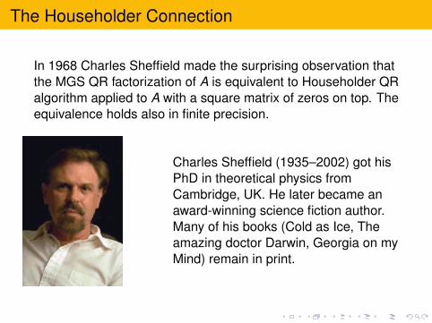
In 1968 Charles Sheffield made the surprising observation thatthe MGS QR factorization of A is equivalent to Householder QRalgorithm applied to A with a square matrix of zeros on top. Theequivalence holds also in finite precision.
Charles Sheffield (1935–2002) got hisPhD in theoretical physics fromCambridge, UK. He later became anaward-winning science fiction author.Many of his books (Cold as Ice, Theamazing doctor Darwin, Georgia on myMind) remain in print.
The Householder Connection
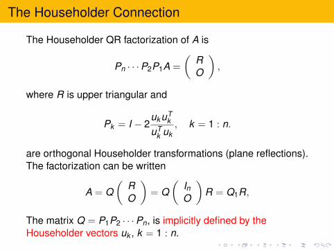
The Householder QR factorization of A is
Pn · · ·P2P1A =
(RO
),
where R is upper triangular and
Pk = I − 2ukuT
k
uTk uk
, k = 1 : n.
are orthogonal Householder transformations (plane reflections).The factorization can be written
A = Q(
RO
)= Q
(InO
)R = Q1R,
The matrix Q = P1P2 · · ·Pn, is implicitly defined by theHouseholder vectors uk , k = 1 : n.
The Householder Connection
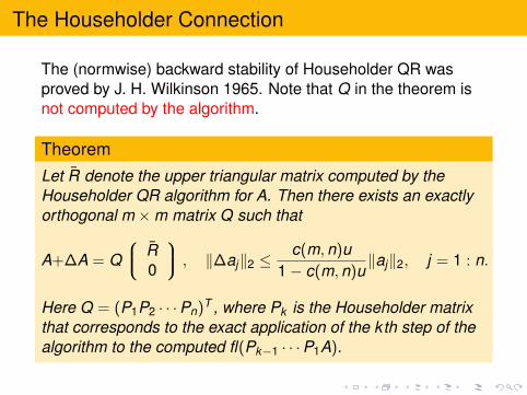
The (normwise) backward stability of Householder QR wasproved by J. H. Wilkinson 1965. Note that Q in the theorem isnot computed by the algorithm.
TheoremLet R denote the upper triangular matrix computed by theHouseholder QR algorithm for A. Then there exists an exactlyorthogonal m ×m matrix Q such that
A+∆A = Q R
0
, ‖∆aj‖2 ≤c(m,n)u
1− c(m,n)u‖aj‖2, j = 1 : n.
Here Q = (P1P2 · · ·Pn)T , where Pk is the Householder matrixthat corresponds to the exact application of the kth step of thealgorithm to the computed fl(Pk−1 · · ·P1A).
The Householder Connection
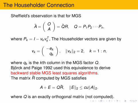
Sheffield’s observation is that for MGS
A =
(OA
)= QR, Q = P1P2 · · ·Pn,
where Pk = I − vkvTk , The Householder vectors are given by
vk =
(−ek
qk
), ‖vk‖2 = 2, k = 1 : n,
where qk is the k th column in the MGS factor Q.Bjorck and Paige 1992 used this equivalence to derivebackward stable MGS least squares algorithms.The matrix R computed by MGS satisfies
A + E = QR, ‖E‖2 ≤ cu‖A‖2.
where Q is an exactly orthogonal matrix (not computed).
Least Squares Algorithms
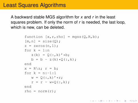
A backward stable MGS algorithm for x and r in the leastsquares problem. If only the norm of r is needed, the last loop,which is new, can be deleted.
function [x,r,rho] = mgss(Q,R,b);[m,n] = size(Q);z = zeros(n,1);for k = 1:n
z(k) = Q(:,k)’*b;b = b - z(k)*Q(:,k);
endx = R\z; r = b;for k = n:-1:1
w = Q(:,k)’*r;r = r - w*Q(:,k);
endrho = norm(r);
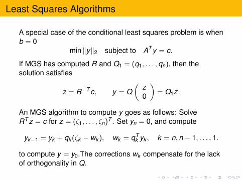
Least Squares Algorithms
A special case of the conditional least squares problem is whenb = 0
min ‖y‖2 subject to AT y = c.
If MGS has computed R and Q1 = (q1, . . . ,qn), then thesolution satisfies
z = R−T c, y = Q(
z0
)= Q1z.
An MGS algorithm to compute y goes as follows: SolveRT z = c for z = (ζ1, . . . , ζn)T . Set yn = 0, and compute
yk−1 = yk + qk (ζk − wk ), wk = qTk yk , k = n,n − 1, . . . ,1.
to compute y = y0.The corrections wk compensate for the lackof orthogonality in Q.
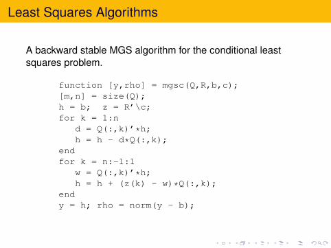
Least Squares Algorithms
A backward stable MGS algorithm for the conditional leastsquares problem.
function [y,rho] = mgsc(Q,R,b,c);[m,n] = size(Q);h = b; z = R’\c;for k = 1:n
d = Q(:,k)’*h;h = h - d*Q(:,k);
endfor k = n:-1:1
w = Q(:,k)’*h;h = h + (z(k) - w)*Q(:,k);
endy = h; rho = norm(y - b);
Software
A multiple purpose orthonormalizing code in 1954 at theNational Bureau of Standards (NBS) is described by Davis andRabinowitz. This used CGS (with a twist). An Algolimplementation named ORTHO by Walsh 1962 includesreorthogonalization and was much used.
In the late 1950th many computer codes for solving leastsquares problems used MGS with column pivoting.Bjorck 1968 published two Algol subroutines for the solution oflinear least squares problems based on MGS. They usedcolumn pivoting and handled the more general least squaresproblem with (consistent) linear equality constraints
minx‖A2x − b2‖2 subject to A1x = b1.
Software
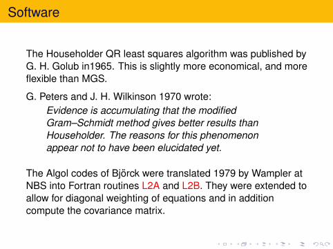
The Householder QR least squares algorithm was published byG. H. Golub in1965. This is slightly more economical, and moreflexible than MGS.
G. Peters and J. H. Wilkinson 1970 wrote:Evidence is accumulating that the modifiedGram–Schmidt method gives better results thanHouseholder. The reasons for this phenomenonappear not to have been elucidated yet.
The Algol codes of Bjorck were translated 1979 by Wampler atNBS into Fortran routines L2A and L2B. They were extended toallow for diagonal weighting of equations and in additioncompute the covariance matrix.
Outline
Early History
Classical versus Modified Gram–Schmidt
Loss of Orthogonality
Least Squares Problems
The Householder Connection
Krylov Subspace Methods
Krylov Subspace Methods
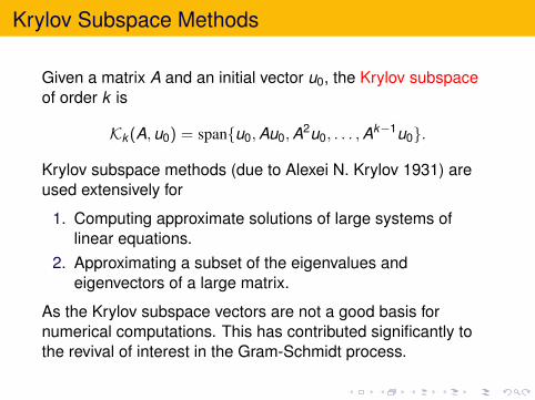
Given a matrix A and an initial vector u0, the Krylov subspaceof order k is
Kk (A,u0) = span{u0,Au0,A2u0, . . . ,Ak−1u0}.
Krylov subspace methods (due to Alexei N. Krylov 1931) areused extensively for
1. Computing approximate solutions of large systems oflinear equations.
2. Approximating a subset of the eigenvalues andeigenvectors of a large matrix.
As the Krylov subspace vectors are not a good basis fornumerical computations. This has contributed significantly tothe revival of interest in the Gram-Schmidt process.
The Arnoldi Method
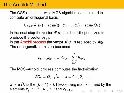
The CGS or column-wise MGS algorithm can be used tocompute an orthogonal basis.
Kk+1(A,u0) = span{q0,q1, . . . ,qk} = span{Qk}
In the next step the vector Aku0 is to be orthogonalized toproduce the vector qk+1.In the Arnoldi process the vector Aku0 is replaced by Aqk .The orthogonalization step becomes
hk+1,kqk+1 = Aqk −k∑
i=1
hikqi .
The MGS–Arnoldi process computes the factorization
AQk = Qk+1Hk , k = 0,1,2, . . . ,
where Hk is the (k + 1)× k Hessenberg matrix formed by theelements hij , i = 1 : k , j ≥ i and hk+1,k
The Arnoldi Method
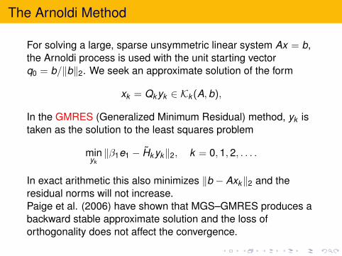
For solving a large, sparse unsymmetric linear system Ax = b,the Arnoldi process is used with the unit starting vectorq0 = b/‖b‖2. We seek an approximate solution of the form
xk = Qkyk ∈ Kk (A,b),
In the GMRES (Generalized Minimum Residual) method, yk istaken as the solution to the least squares problem
minyk‖β1e1 − Hkyk‖2, k = 0,1,2, . . . .
In exact arithmetic this also minimizes ‖b − Axk‖2 and theresidual norms will not increase.Paige et al. (2006) have shown that MGS–GMRES produces abackward stable approximate solution and the loss oforthogonality does not affect the convergence.
The Arnoldi Method
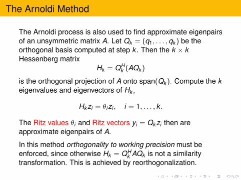
The Arnoldi process is also used to find approximate eigenpairsof an unsymmetric matrix A. Let Qk = (q1, . . . ,qk ) be theorthogonal basis computed at step k . Then the k × kHessenberg matrix
Hk = QHk (AQk )
is the orthogonal projection of A onto span(Qk ). Compute the keigenvalues and eigenvectors of Hk ,
Hkzi = θizi , i = 1, . . . , k .
The Ritz values θi and Ritz vectors yi = Qkzi then areapproximate eigenpairs of A.
In this method orthogonality to working precision must beenforced, since otherwise Hk = QH
k AQk is not a similaritytransformation. This is achieved by reorthogonalization.
Reorthogonalization
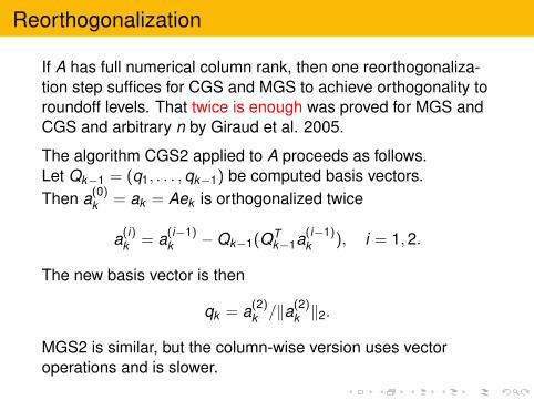
If A has full numerical column rank, then one reorthogonaliza-tion step suffices for CGS and MGS to achieve orthogonality toroundoff levels. That twice is enough was proved for MGS andCGS and arbitrary n by Giraud et al. 2005.
The algorithm CGS2 applied to A proceeds as follows.Let Qk−1 = (q1, . . . ,qk−1) be computed basis vectors.Then a(0)
k = ak = Aek is orthogonalized twice
a(i)k = a(i−1)
k −Qk−1(QTk−1a(i−1)
k ), i = 1,2.
The new basis vector is then
qk = a(2)k /‖a(2)
k ‖2.
MGS2 is similar, but the column-wise version uses vectoroperations and is slower.
Acknowledgements
Steven J. Leon, Ake Bjorck, and Walter Gander.Gram–Schmidt Orthogonalization: 100 Years and More.SIAM Review, submitted 2009.


![Gram–Schmidt–Fisher scoring algorithm for parameter … · ) is called Fisher (expected) Information matrix˜ and its inverse, for ˜ ( ˚ )= [ I ( ˚ )] −1 gives the asymptotic](https://img.pdfslide.us/doc/110x75/5c2aea7a09d3f212718bf837/gramschmidtfisher-scoring-algorithm-for-parameter-is-called-fisher-expected.jpg)