Gradual Land-use Change in New Zealand: Results from a Dynamic

Econometric Model Suzi Kerr and Alex Olssen

Motu Working Paper 12-06 Motu Economic and Public Policy Research

May 2012

i

Author contact details Suzi Kerr Motu Economic and Public Policy Research suzi.kerr@motu.org.nz

Alex Olssen Motu Economic and Public Policy Research alex.olssen@motu.org.nz

Acknowledgements We would like to thank Max Aufhammer from the University of California Berkeley for suggestions made when an earlier draft of this paper was presented there. We would like to thank Arthur Grimes for many useful discussions about the time series analysis. We are also grateful for comments received at the New Zealand Agricultural and Resource Economics Society conference in 2011. Funding from the Ministry of Science and Innovation through the Integrated Economics of Climate Change Program is also gratefully acknowledged. Of course, all remaining errors are our own.

Motu Economic and Public Policy Research PO Box 24390 Wellington New Zealand

Email info@motu.org.nz Telephone +64 4 9394250 Website www.motu.org.nz

© 2012 Motu Economic and Public Policy Research Trust and the authors. Short extracts, not exceeding two paragraphs, may be quoted provided clear attribution is given. Motu Working Papers are research materials circulated by their authors for purposes of information and discussion. They have not necessarily undergone formal peer review or editorial treatment. ISSN 1176-2667 (Print), ISSN 1177-9047 (Online).

ii

Abstract Rural land use is important for New Zealand’s economic and environmental outcomes. Using a dynamic econometric model and recent New Zealand data, we estimate the response of land use to changing economic returns as proxied by relevant commodity prices. Because New Zealand is small, export prices are credibly exogenous. We show that land use responses can be slow. Our result implies that policy-induced land-use change is likely to be slow or costly.

JEL codes Q15, Q24

Keywords Land use, New Zealand, time series

iii

Contents

1.  Introduction ........................................................................................................................................ 4 

2.  Theoretical framework ...................................................................................................................... 6 

3.  Data ...................................................................................................................................................... 8 

3.1  Land area data ................................................................................................................ 8 

3.2  Commodity price and export unit value data ............................................................ 9 

3.3  Time series graphs ....................................................................................................... 10 

4.  Econometric methodology ............................................................................................................. 11 

4.1  Unit root tests .............................................................................................................. 11 

4.2  Cointegration tests....................................................................................................... 12 

4.3  Dynamic specification................................................................................................. 14 

5.  Results ............................................................................................................................................... 15 

5.1  Estimation of the general dynamic model ............................................................... 16 

5.2  Testing dynamic simplifications ................................................................................ 18 

6.  Land use responses to a permanent price change ....................................................................... 18 

7.  Conclusion ........................................................................................................................................ 20 

8.  References ......................................................................................................................................... 22 

9.  Appendix ........................................................................................................................................... 24 

Figures and Tables

Figure 1: Sheep-beef land use and prices, 1974–2005 ........................................................................... 4 

Figure 2: Share of rural land by use, 1973–2005 .................................................................................. 10 

Figure 3: Real prices (standardised), 1973–2005 .................................................................................. 11 

Table 1: Unit root tests ............................................................................................................................ 12 

Table 2: Auxiliary long-run model for cointegration tests .................................................................. 13 

Table 3: General dynamic model coefficient estimates ....................................................................... 17 

Table 4: Testing dynamic simplifications .............................................................................................. 18 

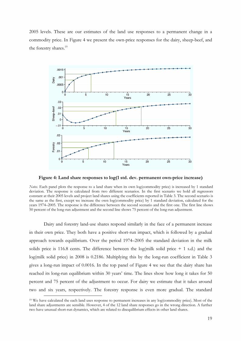
Figure 4: Land share responses to log(1 std. dev. permanent own-price increase) ......................... 19 

Figure 5: The share of land in horticulture and in other land, 1973–2005 ....................................... 24 

4

1. Introduction

Several reasons for gradual land-use change have been identified and discussed in the

literature, but empirical evidence is limited. In a United States context, Stavins and Jaffe (1990)

and Hornbeck (2009) find that land-use change is slow. Schatzki (2003) finds that landowners

place a high value on the option to convert later, which implies hysteresis in land use choices. In

this paper, using a time series model, we estimate how land use changes in response to relevant

commodity prices in New Zealand where, due to its small size, prices are credibly exogenous;

endogenous prices are a challenge for estimating the response of land use to economic returns in

the United States (e.g. Lubowski, Plantinga, and Stavins (2008)). We estimate a dynamic model of

land-use change. We find that in New Zealand it can take many years before the full land-use

impact of changes in economic returns is realised.

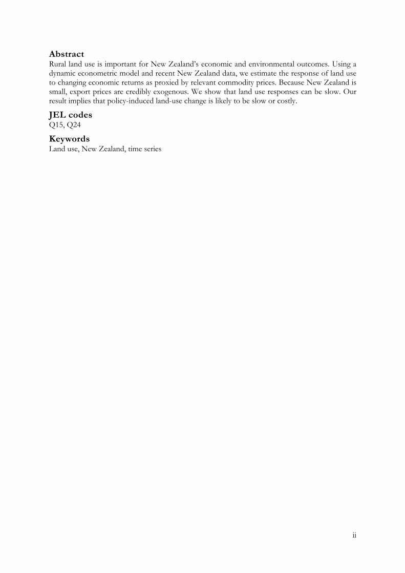
Figure 1 is suggestive of slow land use adjustment. It shows composite sheep-beef prices

and New Zealand’s sheep-beef land share from 1973–2008.1 In 1986 New Zealand removed

large subsidies to sheep meat, beef meat, and wool production. Despite this, the share of land

used for sheep-beef farming stays relatively stable until the mid 1990s.

Figure 1: Sheep-beef land use and prices, 1974–2005

1 Because sheep and beef are often grazed on the same land we cannot separate the two land uses. We use a weighted average of several subsidy-adjusted commodity prices relevant to sheep and beef farming, as explained below.

5

The graph abstracts from many factors affecting land use, including changes in the

returns to competing land uses. This graph is consistent with the idea that large changes in

economic profits need not be followed by instantaneous responses in land use. Land use

responses can be considerably delayed, and they can be gradual. The coefficients from our

dynamic econometric model of land use are also consistent with this idea.

New Zealand rural land is dominated by four major uses: dairy farming, sheep and beef

farming, plantation forestry, and unproductive scrub. Using national time series data we look at

how each of these land uses has responded to changing economic returns, as measured by

relevant commodity prices, over the period from 1974 to 2005.2 We do this by developing a

dynamic econometric model that relates rural land use to economic factors. We follow the

literature on the estimation of dynamic singular equation systems (Anderson and Blundell (1982,

1983)). Singular equation systems have often been estimated to model consumer expenditure

patterns; expenditure and savings always add up to income. We adopt this framework to look at

land use choices; the sum of rural land in each use always adds up the total amount of rural land.

An advantage of estimating the responsiveness of rural land use to economic returns in

New Zealand is that, due to its small size, export prices are credibly exogenous. Furthermore,

large cuts to agricultural supports in 19863 provide an extra source of credibly exogenous

variation in agricultural returns.

Our coefficients provide preliminary estimates of the responsiveness of different types of

rural land to changing economic returns. The small quantity of available data is a potential

problem for our research. However our results are largely consistent with theory. Long-run own-

price elasticities are typically positive, while cross-price elasticities are typically negative.

The rest of this paper is structured as follows. In section 2 we develop a theoretical

model of land-use choice at a parcel level and show what this implies for aggregate land use.

Section 3 describes our data. In section 4 we present our econometric methodology. Section 5

contains estimation results, including our tests of dynamic simplifications. Section 6 looks at land

use responses to permanent increases in relevant commodity prices. It shows that, under the

coefficients we estimate, land use adjustment is slow. In section 7 we conclude.

2 We do not use data from 2006 onwards because we think that land-use change between 2006 and 2008 was partly driven by expectations around New Zealand’s Emissions Trading Scheme particularly relating to forestry, and because since 2008 New Zealand’s Emissions Trading Scheme affected the return to forestry in a way that is difficult to measure directly. 3 McDermott et al., 2008.

6

2. Theoretical framework

In this section we present a dynamic, theoretical model of land use choice between dairy,

sheep-beef, forestry, and scrub; the goal is to provide a framework for thinking about factors

that affect the speed and scale of land-use change in response to changing economic returns.

Our model is close to the models presented in Kerr, Pfaff, and Sanchez-Azofeila (2002) and

Irwin and Bockstael (2002). However we generalise the model to allow for multiple land uses,

because our empirical analysis considers all of New Zealand’s most important rural land uses.

Consider a parcel of land, initially used for sheep-beef farming, that is sufficiently small

that its land quality is homogeneous. Suppose that the annual rent per hectare of land in the -th

use is , use where could be sheep-beef , dairy , forestry , or scrub , the cost of

converting into the -th use is , and the discount rate is .4 We assume land use decisions

are made to maximise the net present value of benefits.

The value at time of converting from sheep-beef into use is

On the other hand, the value at time of delaying conversion a period is

1

Several conditions are necessary for conversion to forestry at time to be optimal; in a

general model with potential conversion options there are 2 necessary conditions for optimal

conversion. Let us restrict attention to a simpler example where the only alternatives to sheep-

beef are forestry and dairy. In that case, we need 2 4 conditions for forestry conversion to be

optimal.

Firstly, forestry conversion at time must be profitable.

0

4 Forestry returns are only realised at the end of a rotation. However, for the theory we can think of the rent as the annualised return.

7

Secondly, forestry conversion must be more profitable than dairy conversion at time .

0

Finally, forestry conversion at time must be more profitable than forestry or dairy conversion

at time 1; this gives two conditions.

1

1

These two inequalities result from comparing the return to forestry conversion at time to the

return to forestry or dairy conversion at time 1. The returns from 1 onwards are

identical for immediate forestry conversion and delayed forestry conversion. When forestry

conversion is immediate, the owner gains the difference in forestry and sheep-beef rents at time

, and pays the conversion costs at time . When conversion is delayed, the owner receives the

sheep-beef returns at time and pays the conversion costs a period later. For delayed dairy

conversion the conversion costs differ. Returns from 1 onwards also differ and this is

reflected by the term under the summation.

If we assume, as in Lubowski, Plantinga, and Stavins (2008), that land managers form

expectations about future rents on the basis of current and historical information, then these

conditions are also sufficient for optimal conversion. If rents follow a random walk, then such a

method of forming expectations is rational.

In this model conversion to forestry becomes more likely as forestry rents increase;

increasing rents makes all of the inequalities necessary for conversion more likely to hold.

Conversion costs can also drive land-use change. Falling conversion costs could result in some

parcels, which could profitably convert immediately, delaying conversion to take advantage of

lower future conversion costs. Other parcels may convert only because of the falling conversion

costs. Increasing economic returns could induce conversion costs to rise temporarily because of

supply-side constraints and fall in the long term because of learning effects. Thus a one-off

change in rents can induce optimal conversion at a later time.

We econometrically model land use at the national level, however the results from the

theoretical model are derived for a parcel of land of homogenous quality. Different quality land

8

will result in different potential rents and hence different optimal land use decisions. National-

level land use is the result of aggregating the land use decisions on smaller parcels.

3. Data

We need two main types of data: data on the area of land in each rural use, and data on

economic variables that we expect to be associated with land use.

3.1 Land area data

We use national level land area data from Statistics New Zealand’s (SNZ) Agricultural

Production Survey supplemented with an independent survey by Meat and Wool Economic

Service (MWES), now known as Beef and Lamb. SNZ provides data on New Zealand’s total

rural land area, as well as the land area in pasture,5 plantation forestry, and horticulture for 1972–

1996 and 2002–2005.6 SNZ did not collect data in 1997, 1998, 2000, or 2001. Furthermore the

1999 survey used a different population base to other years and so we exclude it. We interpolate

the plantation forestry area for these years. We do this as follows. We find the net change in

forestry over the period. We then find a second source of data on national level plantation

forestry area, the Ministry of Agriculture and Forestry’s (now the Ministry for Primary

Industries) National Exotic Forestry Description reports. From this data source, we calculate the

annual proportions of the total change in forest area between 1996 and 2002. We use these

proportions to allocate the total change in the SNZ data.

The MWES data covers the period 1980–2005, including the period 1997–2001 when

SNZ did not collect land area data. MWES splits pasture between dairy land, sheep-beef land,

and other agricultural land. We extrapolate their dairy area series back to 1972. In particular, we

regress the dairy area from 1980–2005 on time, total dairy cattle numbers from SNZ, and an

interaction of time and cattle numbers; this will capture changes in stocking rates over time. We

then estimate the change in the dairy area from year to year using the coefficients from this

regression and data on dairy cattle numbers back to 1972. This enables us to extrapolate the dairy

land area back to 1972. We use the remaining pasture land as our measure of sheep-beef land.7

5 On www.stats.govt.nz/infoshare this is the grazing area, or the sum of grassland, lucerne, tussock, and danthonia (sometimes the grazing area is reported, and sometimes only the other categories are reported, but whenever they all are recorded the sum of the other categories is equal to the grazing area). 6 The population that was sampled has changed over time. Prior to 1994 it included all business recorded on SNZ’s Business Directory engaged in horticulture, cropping, livestock farming, or exotic forestry operations. From 1994 to 1996 only GST registered businesses were included. Currently all businesses involved in agricultural, horticultural, or forestry production are included. 7 This includes land used for deer and goat farming. However the relevant areas are trivially small.

9

This gives us land area data for three of the four major rural New Zealand land uses. We

define scrub, the last major use, to be the difference between the total rural land area and the

land area in pasture, plantation forestry, or horticulture.8 Finally, the total amount of rural land in

New Zealand has been typically shrinking over the period we study. We calculate all land-use

shares relative to total rural land in 1973. We then define the area of ‘other land’ in any given

year to be the difference between total rural land in 1973 and the sum of land in rural uses in that

year. In our model the addition of one hectare of sheep-beef land has no effect on the

relationship between dairy prices and dairy land. Thus we define our land shares with respect to

1973 rural land because otherwise changes in the amount of rural land would automatically

induce changes in every land share.

3.2 Commodity price and export unit value data

We use two main sources of data on commodity prices and export unit values. SNZ

overseas merchandise trade data provides information on the value, in New Zealand dollars

(NZD), and volume of exports for beef meat, sheep meat, wool, and logs.9 We use this data to

calculate export unit values for sheep meat, beef meat, wool, and logs. Milk solids prices are

from the Livestock Improvement Corporation.

New Zealand has a history of strong agricultural assistance. Anderson et al. (2007)

estimates positive levels of support provided for sheep meat, beef meat, wool, and dairy until

1990. We want our export unit values and prices to be an exogenous measure of the economic

return to each productive rural land use. If we ignored agricultural assistance, then our export

unit values and prices could not be expected to give a good measure of relative economic returns

across land uses, or across time. Thus we use the Anderson et al. (2007) estimates to adjust our

export unit values and prices for the relevant period.

Finally, because we have only 32 years of data, and we want to estimate a dynamic model,

which requires lagged variables to enter our estimating equation, we are severely restricted in

terms of our degrees of freedom. To address this problem, we make a composite sheep-beef

export unit value, which allows us to avoid entering sheep meat, beef meat, and wool export unit

values, as well as their lags, into our regressions separately. Our composite export unit value in

any year is simply the average of the individual export values, weighted by export volume in the

8 Horticultural area must be interpolated for 1972–1982 and 1997–2001. We use simple regressions of the area in horticulture on time. 9 These series are available from www.stats.govt.nz/infoshare  from 1989 July to 2008 June. Our beef meat data corresponds to Harmonized Commodity Description and Coding System groups HS0201–HS0202. Sheep meat data is from HS020410–HS020443. Wool data is from HS5101. The log data for export unit values are from the Ministry of Agriculture and Fisheries (MAF); recent data can be found at http://www.maf.govt.nz/news-resources/statistics-forecasting/forestry/annual-forestry-export-statistics.aspx. We use the series for logs and poles.

10

same year. We also use five year nominal interest rates from the Reserve Bank of New Zealand

as a macroeconomic indicator.

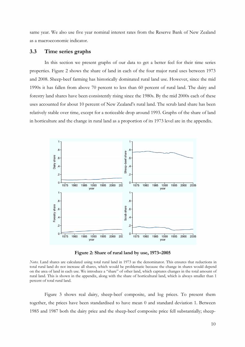
3.3 Time series graphs

In this section we present graphs of our data to get a better feel for their time series

properties. Figure 2 shows the share of land in each of the four major rural uses between 1973

and 2008. Sheep-beef farming has historically dominated rural land use. However, since the mid

1990s it has fallen from above 70 percent to less than 60 percent of rural land. The dairy and

forestry land shares have been consistently rising since the 1980s. By the mid 2000s each of these

uses accounted for about 10 percent of New Zealand’s rural land. The scrub land share has been

relatively stable over time, except for a noticeable drop around 1993. Graphs of the share of land

in horticulture and the change in rural land as a proportion of its 1973 level are in the appendix.

Figure 2: Share of rural land by use, 1973–2005

Notes. Land shares are calculated using total rural land in 1973 as the denominator. This ensures that reductions in total rural land do not increase all shares, which would be problematic because the change in shares would depend on the area of land in each use. We introduce a “share” of other land, which captures changes in the total amount of rural land. This is shown in the appendix, along with the share of horticultural land, which is always smaller than 1 percent of total rural land.

Figure 3 shows real dairy, sheep-beef composite, and log prices. To present them

together, the prices have been standardised to have mean 0 and standard deviation 1. Between

1985 and 1987 both the dairy price and the sheep-beef composite price fell substantially; sheep-

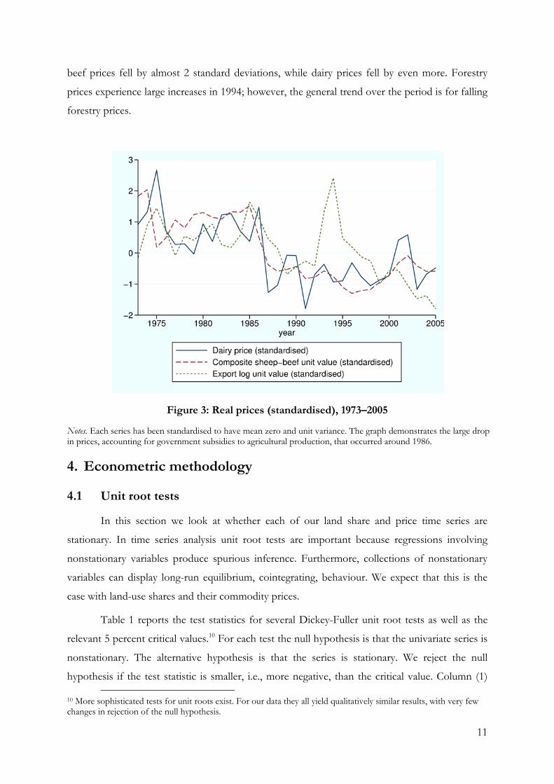
11

beef prices fell by almost 2 standard deviations, while dairy prices fell by even more. Forestry

prices experience large increases in 1994; however, the general trend over the period is for falling

forestry prices.

Figure 3: Real prices (standardised), 1973–2005

Notes. Each series has been standardised to have mean zero and unit variance. The graph demonstrates the large drop in prices, accounting for government subsidies to agricultural production, that occurred around 1986.

4. Econometric methodology

4.1 Unit root tests

In this section we look at whether each of our land share and price time series are

stationary. In time series analysis unit root tests are important because regressions involving

nonstationary variables produce spurious inference. Furthermore, collections of nonstationary

variables can display long-run equilibrium, cointegrating, behaviour. We expect that this is the

case with land-use shares and their commodity prices.

Table 1 reports the test statistics for several Dickey-Fuller unit root tests as well as the

relevant 5 percent critical values.10 For each test the null hypothesis is that the univariate series is

nonstationary. The alternative hypothesis is that the series is stationary. We reject the null

hypothesis if the test statistic is smaller, i.e., more negative, than the critical value. Column (1)

10 More sophisticated tests for unit roots exist. For our data they all yield qualitatively similar results, with very few changes in rejection of the null hypothesis.

12

and column (2) provide evidence that most of our series are nonstationary in levels. In column

(1) we marginally reject nonstationarity only for the forestry share and the log(dairy price) series.

However, Figure 1 suggests the presence of trends in our land share time series. In column (2)

we allow for trends in our time series. In this case, we can reject nonstationarity only for the

log(dairy price) series.

Although our series mostly appear to be nonstationary in levels, we can reject the null

nonstationarity when we take first differences. Apart from the first difference in the forestry

share, all other differenced series have test statistics considerably more negative than the critical

values. Thus, for the rest of this paper we proceed under the assumption that our series are

indeed stationary in differences.

Table 1: Unit root tests

Levels First differences (1) (2) (3) (4)

dairy share 0.843 -2.656 -3.901 -3.968 sheep-beef share 1.942 -1.022 -4.420 -5.550 forestry share -2.265 1.415 -0.659 -1.167 scrub share -0.806 -1.623 -4.249 -4.175 other share 2.240 -2.804 -3.235 -5.647 log(dairy price) -3.077 -4.225 -7.476 -7.346 log(sheep-beef price) -1.638 -1.766 -5.341 -5.294 log(forestry price) -1.639 -2.846 -5.374 -5.465 interest rate -1.292 -2.264 -4.513 -4.761 critical value 5% -2.98 -3.56 -2.98 -3.56 Notes. This table reports test statistics for Dickey-Fuller unit root tests on each univariate time series used in our analysis. The null hypothesis is that the univariate series is stationary. Each cell reports a separate test statistics; the row identifies the dependent variable and the column identifies the specific test. Columns (2) and (4) allow for trends, while columns (1) and (3) do not.

4.2 Cointegration tests

Given our time series are stationary in differences it is natural to ask whether some

combination of them are stationary in levels. In other words, we want to know if there are

cointegrating factors that would allow us to think of a combination of our time series as having

equilibrium tendencies.

To answer this question, we test for cointegration. We estimate

1

13

where is the share of land in use at time , is the price (we demean, after taking logs) of

the -th commodity at time 1,11 is the nominal 5 year interest rate, is the share of other

land, is the error term, and , , , and are parameters to be estimated. The results

from estimating these equations by OLS are shown in Table 2 below.

Table 2: Auxiliary long-run model for cointegration tests

dairy sheep-beef forestry Scrub dairy price 0.002 -0.015 -0.002 0.016

(0.004) (0.009) (0.007) (0.010) sheep-beef price -0.019*** 0.027*** -0.054*** 0.046***

(0.003) (0.008) (0.006) (0.010) forestry-price 0.013*** 0.030*** 0.012** -0.056 ***

(0.004) (0.009) (0.006) (0.010) other land share 0.520*** -1.480*** 0.608 *** -0.647 ***

(0.028) (0.070) (0.049) (0.077) interest rates 0.001*** -0.004*** 0.003*** 0.000

(0.000) (0.001) (0.000) (0.000) constant 0.086*** 0.705*** 0.078 *** 0.131***

(0.001) (0.001) (0.001) (0.001) Notes. Standard errors are in parentheses. Each column reports the coefficient from estimating a single equation model by OLS. The dependent variable is the column title. Each row reports coefficients for the relevant regressor. Commodity price variables are demeaned, after taking logs. * / ** / *** significant at the 10 / 5 / 1 percent level respectively.

Using the residuals from these regressions, we test for cointegration. We use two panel

unit root tests.12 One test is based on Choi (2001) and requires only ∞ asymptotics. The

null hypothesis is that the residuals of all equations are nonstationary, and the alternative

hypothesis is that at least one equation is stationary. This does not test cointegration directly, but

it uses appropriate asymptotics; if we cannot reject the null hypothesis this would be evidence

against cointegration. The second test is based on Hadri (2000). It requires ∞ and then

∞. Given we are only interested in four land uses this may not be appropriate. On the

other hand the null hypothesis is appropriate. Under the null hypothesis the residuals of all

11 Because land use decisions depend on expected future profitability under different uses, lagged prices are often used to account for expectations formation; for example, see footnote 5 of Miller and Plantinga (1999). 12 We used information from the [xt] xtunitroot section of the Stata’s User Manual throughout this section.

14

equations are stationary, while under the alternative hypothesis the residuals of at least one of the

equations are nonstationary. Together we take these tests are indicative of cointegration.13

We implement these tests using residuals obtained by estimating ( 1 ). Because the fourth

use is completely determined given the other three rural land shares and the amount of other

land, we omit one series in these panel unit root tests. We demean the residuals and run separate

specifications with no lags, one lag or two lags. Using Choi’s method we reject the null

hypothesis that all residual series have nonstationary at the 5 or 10 percent level for any lags; the

results of this test do not rule out cointegration. Using Hadri’s method we fail to reject the null

hypothesis that all residual series are stationary at even the 10 percent level using any of the

above number of lags; this is also consistent with cointegration. We take this as evidence that our

variables are cointegrated and that there is a cointegrating factor which means the system

represents a long-run equilibrium relationship. As such, we proceed to develop a dynamic

econometric model, which has a structure that closely resembles an error correction model.

4.3 Dynamic specification

We want to estimate the relationship between land use and commodity prices. In

particular, using national level time series data, we want to see how land use changes as

commodity prices change. In terms of the theoretical framework outlined above, we can think of

each land owner varying her allocation of land to each use to maximise her profit. In a stochastic

world the land owner must form expectations about future returns under each land use. At a

national level, the land area in each rural use is the result of aggregating these individual profit

maximising decisions. These land areas can also be expressed as shares of total rural land. The

share of land in each use depends on the expected returns to rural production in all uses. When

the set of uses considered is exhaustive and mutually exclusive, such a system of equations is

necessarily singular. We have four rural land uses.14 Thus, given three of the rural land shares, we

can infer the fourth.

Dynamic considerations play an important role in our econometric specification. Land

use decisions made now impact future options and profitability; for example, because of

conversion costs. This means that responses to economic conditions may have dynamic effects.15

Anderson and Blundell (1982) developed a methodology for incorporating general dynamics in

13 These tests are both unit root tests. Although we are testing cointegration, and we have used multiple regressors in the first stage regression used to calculate the residuals, we have made no adjustment to the p-values. 14 Five if you include exogenous other land. 15 In consumer expenditure modelling, the major field for the estimation of share equation systems, static models were often found to reject fundamental properties of consumer theory. Appropriate allowance for dynamics substantially reduced rejection rates. This would be consistent with habit formation, for example. In a land use setting dynamics are arguably even more important.

15

singular system estimation.16 Their method attractively nests several dynamic simplifications

allowing researchers to test whether a static model really is rejected by the data.

Given the long-run cointegrating relationship established in the previous section we

specify our general dynamic model as

∆ ∆ 2

where, as analogues to Anderson and Blundell (1982), ∆ is a vector of the changes in each of

four land uses between time and time 1, is a matrix containing the variables that go

into the long run equation above at time 1, and is the same as with the column for the

constant removed. specifies the long-run structure, specifies the short-run structure, and

is a matrix that contains combinations of adjustment coefficients. The adjustment coefficients

are not individually identified. We cannot recover them from , which contains only

combinations of them. For details see Anderson and Blundell (1982). However all aspects of the

long run structure are identified.

Because this system of equations is singular, estimation requires us to omit one of the

land shares. We estimate the system by iterated nonlinear generalised least squares using Stata.

These estimates are numerically equivalent to the maximum likelihood estimates,17 which have

the desirable property of being invariant to the land share omitted, even when restrictions are

imposed on the model.

5. Results

In this section we present results from our econometric estimation. Firstly we report

estimates for our general dynamic framework. Following that we test against several popular

dynamic simplifications. In the general specification we find that most of the long-run responses

of land shares to price changes are as expected. Own price elasticities are positive and cross price

elasticities are mostly negative. The short-run responses tell a different story. Almost all

productive land shares increase when any prices increase, and the share of land in unproductive

scrub decreases as any prices increase. This suggests that there may be other factors driving the

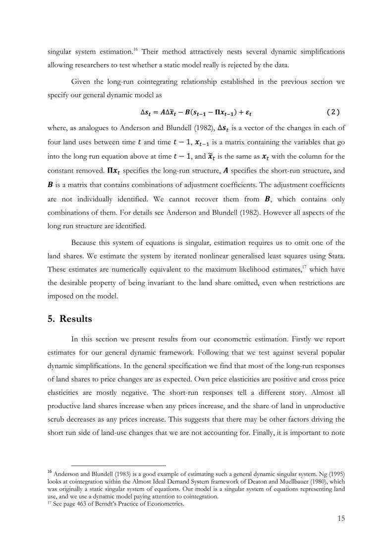
short run side of land-use changes that we are not accounting for. Finally, it is important to note

16 Anderson and Blundell (1983) is a good example of estimating such a general dynamic singular system. Ng (1995) looks at cointegration within the Almost Ideal Demand System framework of Deaton and Muellbauer (1980), which was originally a static singular system of equations. Our model is a singular system of equations representing land use, and we use a dynamic model paying attention to cointegration. 17 See page 463 of Berndt’s Practice of Econometrics.

16

that most of our coefficients lack statistical significance. This is not surprising given we have

little and noisy data.

5.1 Estimation of the general dynamic model

We estimate the general dynamic model in equation ( 2 ) using feasible iterated

generalised least squares. Our results are presented in Table 3. Looking at the long-run price

responsiveness we see that most shares are estimated to increase as their own commodity price

increases and to decrease as competing commodity prices increase. There are three exceptions;

the dairy share is positively associated with forestry prices, the scrub share is positively associated

with dairy prices, and the scrub share is positively associated with sheep-beef prices. The dairy

share, forestry price association is something that comes through strongly in the data. We do not

think this represents a causal relationship. The scrub share, commodity price relationships are

also unusual. While these estimates have unusual signs none of them are estimated as differing

from zero at conventional levels of statistical significance. We may simply lack enough data to

get good estimates of the relationships of interest.

The short-run price relationships are also interesting. The change in land share for all

productive uses is estimated to increase as any commodity price increases. All changes in

commodity prices are estimated to have negative coefficients in the scrub share equation. Thus

there appears to be a split in the short run between productive and unproductive use. This also

suggests there could be an important omitted variable from our estimating equation. In

particular, we are only capturing one source of the variation in economic returns; omission of

other important variables that affect economic returns could bias our estimates.

We have estimated several other specifications; however, none of them resolved this.18

We included Gross Domestic Product; we thought that changes in domestic output might be

linked with credit availability and hence to short-run land-use change. We included building

expenditure for manufacturing, with the idea that this expenditure would be higher in

environments that were favourable for investment. We also tried including exchange rates. The

results were similar when the NZD/GBP exchange rate was included; however the model had

convergence problems when the NZD/USD exchange rate was used.

18 Unsurprisingly, given the amount of data we have, the estimates are reasonably sensitive to the changes in the specification. Results from alternative specifications can be obtained from the authors.

17

Table 3: General dynamic model coefficient estimates

Change in land use i

Constant

log(lagged dairy price)

log(lagged sheep-beef

price)

log(lagged forestry price)

Lagged other land

Lagged interest

rates

Change in log(dairy

price)

Change in log(sheep

-beef price)

Change in log(forestry price)

Change in other land

Change in interest

ratesBi1 Bi2 Bi3

Dairy 0.080*** 0.007 -0.053** 0.063 0.495*** 0.002*** 0.000 0.008** 0.006** 0.018 0.000 0.545*** -0.042 -0.331***

(0.012) (0.015) (0.026) (0.049) (0.093) (0.001) (0.002) (0.003) (0.002) (0.070) (0.000) (0.135) (0.034) (0.067)

Sheep-beef

0.719*** -0.041* 0.106** -0.099 -1.478*** -0.006*** 0.004 0.029** 0.021*** -1.151*** -0.002** 1.198* 0.417*** -0.111 (0.020) (0.024) (0.042) (0.079) (0.151) (0.001) (0.009) (0.014) (0.001) (0.284) (0.001) (0.614) (0.137) (0.273)

Forestry 0.062*** 0.013 -0.102* 0.102 0.578*** 0.004*** 0.001 0.000 0.005*** -0.087** 0.000 0.060 -0.048*** -0.016 (0.025) (0.030) (0.053) (0.101) (0.192) (0.002) (0.001) (0.001) (0.001) (0.035) (0.000) (0.076) (0.017) (0.034)

Scrub 0.139 0.020 0.050 -0.067 -0.586 0.001 -0.006 -0.037 -0.032 0.220 0.002 -1.803 -0.327 0.459

(-) (-) (-) (-) (-) (-) (-) (-) (-) (-) (-) (-) (-) (-) Notes. Standard errors are in parentheses. The coefficients are the result of estimating a dynamic singular equation system following Anderson and Blundell (1982). The system contains four equations and hence has four dependent variables; dairy, sheep-beef, forestry, and scrub land shares, which each have a separate row in the table. All commodity price variables are demeaned, after taking logs. Each column reports the coefficients for a separate regressor. The lagged variables correspond to the long-run structure, while the differenced variables correspond to the short-run structure. The coefficients correspond to combinations of adjustment parameters that are not separately identified; see Anderson and Blundell (1982). * / ** / *** significant at the 10 / 5 / 1 percent level respectively (no finite-sample correction used). The coefficients in the scrub equation are backed-out from the adding up constraints. We omit their standard errors (-).

18

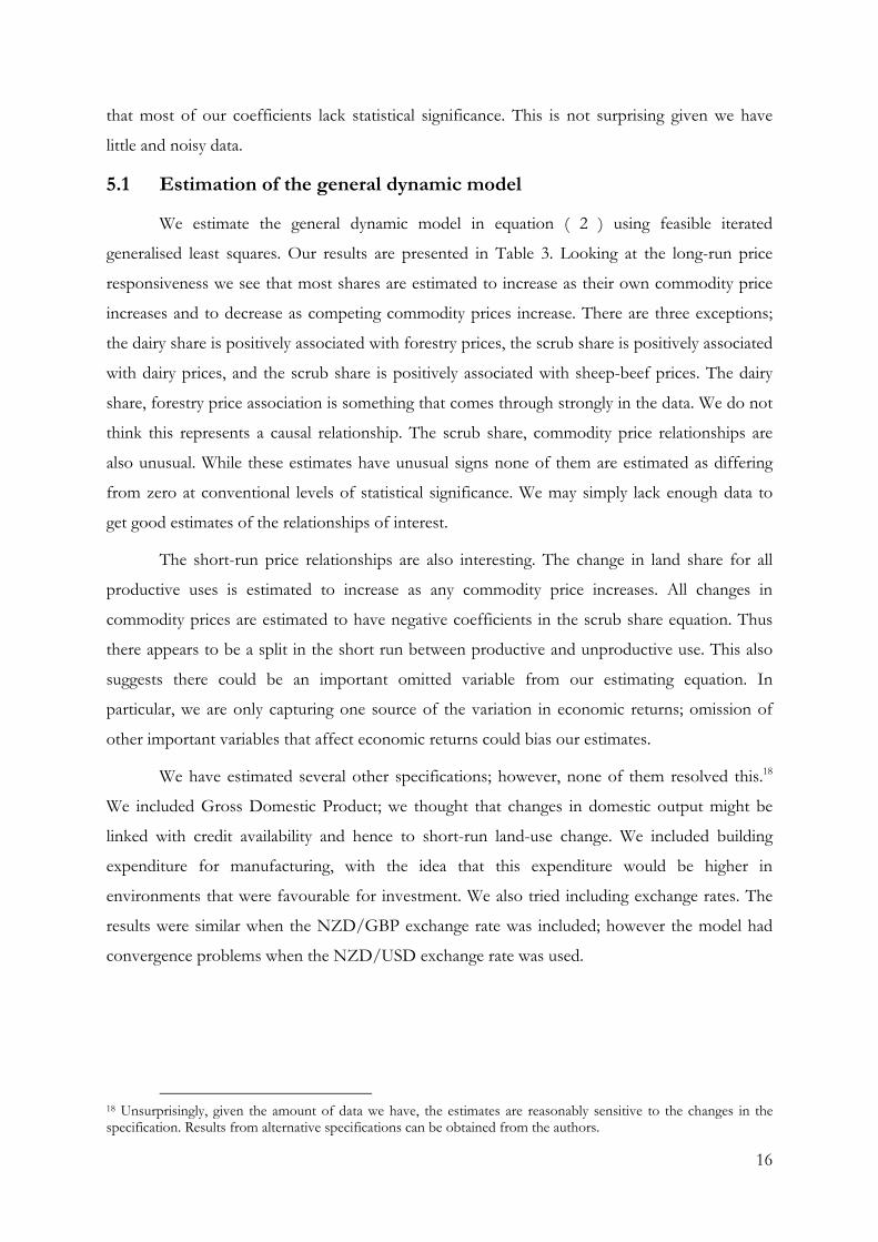
5.2 Testing dynamic simplifications

The dynamic specification of our model is likely to be important because land use

choices now affect future land use profitability. Several simpler dynamic structures are nested in

our general model and can be implemented by appropriate coefficient restraints. In particular

Anderson and Blundell (1982) showed the coefficient restrictions necessary to collapse the

general model to either an AR(1) model, a partial adjustment model, or a static model. Consider

equation ( 2 ). Denote the elements of a matrix by lower case letters. If for all and ,

then we get the AR(1) model. If each ∑ , then we get the partial adjustment

model. From either the AR(1) model or the partial adjustment model we can get the static model

by constraining where is the Kronecker delta.

Table 4: Testing dynamic simplifications

AR(1) PA Static Static

Degrees of freedom 15 15 9 9

Likelihood-ratio statistic 50.2* 42.3* 148.7* 156.6* Critical value 1% 30.6 30.6 21.7 21.7 Notes. The table reports the results of likelihood-ratio tests of dynamic simplifications. Column 1 compares the dynamic model in Table 3 with an AR(1) model. Column 2 compares the model in Table 3 with a partial adjustment model. Columns 3 and 4 compare the AR(1) and partial adjustment models respectively with a static model.

We test each of these dynamic simplifications in turn using likelihood ratio tests. Our

results are presented in Table 4. Column 1 reports the test for the general model against the

AR(1) model; column 2 gives results for the general model against the partial adjustment model.

The AR(1) model and the partial adjustment models are tested against the static model in

columns 3 and 4 respectively. All simplifications can be rejected at the 1 percent level. The most

general model we consider, which allows the disequilibrium in dairy, sheep-beef, and forestry to

affect all land-use changes, is always preferred in our data.

6. Land use responses to a permanent price change

We run a series of simulations to look at the effect of commodity prices on land use; in

particular we are interested in the speed of adjustment. Firstly, we hold all regressors fixed at

their 2005 levels and calculate the paths of each land-use share into the future. Secondly, we

increase one log(commodity price) by one standard deviation, hold it there for all time, and

calculate the associated paths for land-use shares. We take the difference between the paths with

a permanent increase in a single commodity price and the paths with all regressors fixed at their

19

2005 levels. These are our estimates of the land use responses to a permanent change in a

commodity price. In Figure 4 we present the own-price responses for the dairy, sheep-beef, and

the forestry shares.19

Figure 4: Land share responses to log(1 std. dev. permanent own-price increase)

Notes. Each panel plots the response to a land share when its own log(commodity price) is increased by 1 standard deviation. The response is calculated from two different scenarios. In the first scenario we hold all regressors constant at their 2005 levels and project land shares using the coefficients reported in Table 3. The second scenario is the same as the first, except we increase the own log(commodity price) by 1 standard deviation, calculated for the years 1974–2005. The response is the difference between the second scenario and the first one. The first line shows 50 percent of the long-run adjustment and the second line shows 75 percent of the long-run adjustment.

Dairy and forestry land-use shares respond similarly in the face of a permanent increase

in their own price. They both have a positive short-run impact, which is followed by a gradual

approach towards equilibrium. Over the period 1974–2005 the standard deviation in the milk

solids price is 116.8 cents. The difference between the log(milk solid price + 1 s.d.) and the

log(milk solid price) in 2008 is 0.2186. Multiplying this by the long-run coefficient in Table 3

gives a long-run impact of 0.0016. In the top panel of Figure 4 we see that the dairy share has

reached its long-run equilibrium within 30 years’ time. The lines show how long it takes for 50

percent and 75 percent of the adjustment to occur. For dairy we estimate that it takes around

two and six years, respectively. The forestry response is even more gradual. The standard

19 We have calculated the each land uses response to permanent increases in any log(commodity price). Most of the land share adjustments are sensible. However, 4 of the 12 land share responses go in the wrong direction. A further two have unusual short-run dynamics, which are related to disequilibrium effects in other land shares.

20

deviation of export log unit values over the period 1974–2005 is 3442.4 cents. This gives us a

long-run impact of 0.2863. It takes around 6 years for 50 percent of the forestry adjustment to

take place and around 12 years for 75 percent of the adjustment to take place.

The sheep-beef land-use response has an immediate short-run increase, followed by a

noticeable dip, and then it returns to its equilibrium path. This highlights the fact that the land-

use shares are very interdependent because of the adding up constraint. In particular, the scrub

share increases in the long run in response to an increase in the sheep-beef price. This happens

relatively quickly, and sheep-beef ends up temporarily decreasing to satisfy the adding up

constraint; dairy and forestry shares are always falling in response to an increase in sheep-beef

prices.

This phenomenon of gradual adjustment is typical of all the land share responses.20 In a

partial adjustment setting with only two land uses Stavins and Jaffe (1990) found between 32 and

69 percent of optimal land-use change occurred within five years. Moreover, the percentage of

optimal land-use change occurring within five years was higher for conversion into pasture, than

it was for abandonment to reverting forest. Our results are very similar. Moreover, while our

results are not directly comparable to Hornbeck (2009), they are consistent. Hornbeck looked at

the impact of topsoil lost during the Dust Bowl catastrophe during the 1930s. He found

evidence that crop productivity decreased relative to pasture, and that wheat productivity

decreased relative to hay. He found that there was no statistically significant land-use change

until at least 10 years after the Dust Bowl incident.21 However, most of his estimates are in the

direction that land-use change would be anticipated; even when the magnitude of the point

estimates is too small to be significant. This is consistent with the gradual land use paths we

presented in Figure 4; if we look at land-use shares five years into the simulation, then the

differences may be too small to be statistically significant. In a world with gradual land-use

change, the longer we wait to make the comparison, the more likely we are to detect an effect.

7. Conclusion

In this paper we estimated the relationships between New Zealand’s main rural land uses

and their associated export prices using national time series data. Our time series are quite short;

this means that many coefficients are estimated imprecisely, and some point estimates are

unconvincing. However, most of our coefficients are consistent with standard economic theory.

20 However, recall that disequilibrium in any land share will increase the annual adjustments of all land shares. Thus so long as one share is out of equilibrium the others must all still be adjusting. 21 We are referring to panels A and B of Table 3 in Hornbeck (2009).

21

In the long run all land shares were estimated as being positively associated with the price of

their own products and most were estimated to have a negative relationship with the price of

products from other land uses.

Our estimates confirm that dynamic considerations are important for land use choices

and should not be overlooked in any empirical analysis. Likelihood ratio tests overwhelmingly

reject the static models in favour of the simple dynamic AR(1) and partial adjustment models.

Furthermore both of these models are rejected at the 1 percent level compared to our more

general model.

Most importantly, our coefficient estimates imply that land use adjusts slowly in response

to changes in economic returns as measured by commodity prices. For each of our productive

land uses, it takes at least six years before 75 percent of long-run equilibrium adjustment occurs

in response to an increase in the own-commodity price by one standard deviation. This is

consistent with the results of Stavins and Jaffe (1990) and Hornbeck (2009). If land-use change is

gradual, then adjustments because of climate change, carbon prices, water restrictions, or

nutrient restrictions are likely to be slow or costly.

Future research will focus on two key areas. Firstly, we will look to estimate the dynamic

relationship between land-use shares and commodity prices using a panel of Territorial Authority

level data; Territorial Authorities are similar in size to US counties. This will allow us to include

data on differential land quality and costs across Territorial Authorities. Secondly, we will

investigate the determinants of gradual land use adjustment. An understanding of these

determinants is likely to be useful for developing policy to change land use because it will allow

such policy to target the most important mechanisms.

22

8. References

Anderson, G. J. and R. W. Blundell. 1982. "Estimation and Hypothesis Testing in Dynamic Singular Equation Systems", Econometrica, 50:6, pp. 1559–71.

Anderson, G. J. and R. W. Blundell. 1983. "Testing Restrictions in a Flexible Dynamic Demand System: An Application to Consumers' Expenditure in Canada", Review of Economic Studies, 50:3, pp. 397–410.

Anderson, K.; R. Lattimore; P. Lloyd and D. Maclaren. 2007. "Distortions to Agricultural Incentives in Australia and New Zealand," World Bank Agricultural Distortions Working Paper 09, the World Bank, Washington DC.

Choi, I. 2001. "Unit Root Tests for Panel Data", Journal of International Money and Finance, 20:2, pp. 249–72.

Deaton, A. and J. Muellbauer. 1980. "An Almost Ideal Demand System", American Economic Review, 70:3, pp. 312–26.

Hadri, K. 2000. "Testing for Stationarity in Heterogeneous Panel Data", Econometrics Journal, 3:2, pp. 148–61.

Hornbeck, R. 2009. "The Enduring Impact of the American Dust Bowl: Short and Long-Run Adjustments to Environmental Catastrophe," NBER Working Paper No. 15605, National Bureau of Economic Research, Cambridge, MA.

Irwin, Elena G. and N. E. Bockstael. 2002. "Interacting Agents, Spatial Externalities and the Evolution of Residential Land Use Patterns", Journal of Economic Geography, 2:1, pp. 31–54.

Kerr, Suzi; Alexander S. P. Pfaff and G. Arturo Sanchez-Azofeila. 2002. "The Dynamics of Deforestation: Evidence From Costa Rica," draft paper, Motu Economic and Public Policy Research .

McDermott, A.; C. Saunders; E. Zellman; T. Hope and E. Fisher. 2008. "The Key Elements of Success and Failure in the NZ Sheep Meat Industry From 1980-2007", Research Report. No. 308, Lincoln University Agribusiness and Economics Research Unit, Lincoln.

Miller, Douglas J. and Andrew J. Plantinga. 1999. "Modeling Land Use Decisions With Aggregate Data", American Journal of Agricultural Economics, 81:1, pp. 180–94.

Ng, S. 1995. "Testing for Homogeneity in Demand Systems When the Regressors Are Nonstationary", Journal of Applied Econometrics, 10:2, pp. 147–63.

Ruben, N. L.; J. P. Andrew and N. S. Robert. 2008. "What Drives Land-Use Change in the United States? A National Analysis of Landowner Decisions", Land Economics, 84:4, pp. 529–50.

23

Schatzki, Todd. 2003. "Options, Uncertainty and Sunk Costs:: an Empirical Analysis of Land Use Change", Journal of Environmental Economics and Management, 46:1, pp. 86–105.

Stavins, R. N. and A. B. Jaffe. 1990. "Unintended Impacts of Public Investments on Private Decisions: The Depletion of Forested Wetlands", American Economic Review, 80:3, pp. 337–52.

24

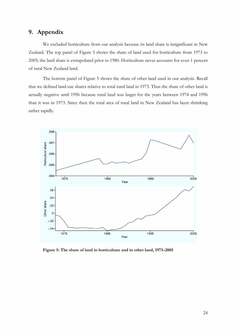
9. Appendix

We excluded horticulture from our analysis because its land share is insignificant in New

Zealand. The top panel of Figure 5 shows the share of land used for horticulture from 1973 to

2005; the land share is extrapolated prior to 1980. Horticulture never accounts for even 1 percent

of rural New Zealand land.

The bottom panel of Figure 5 shows the share of other land used in our analysis. Recall

that we defined land-use shares relative to total rural land in 1973. Thus the share of other land is

actually negative until 1996 because rural land was larger for the years between 1974 and 1996

than it was in 1973. Since then the total area of rural land in New Zealand has been shrinking

rather rapidly.

Figure 5: The share of land in horticulture and in other land, 1973–2005

Recent Motu Working Papers

All papers in the Motu Working Paper Series are available on our website www.motu.org.nz, or by contacting us on

info@motu.org.nz or +64 4 939 4250.

12-05 Abramitzky, Ran, and Isabelle Sin. 2012. “Book Translations as Idea Flows: The Effects of the Collapse of

Communism on the Diffusion of Knowledge”.

12-04 Fabling, Richard, and David C. Maré. 2012. “Cyclical Labour Market Adjustment in New Zealand: The Response of

Firms to the Global Financial Crisis and its Implications for Workers”.

12-03 Kerr, Suzi, and Adam Millard-Ball. 2012. “Cooperation to Reduce Developing Country Emissions”.

12-02 Stillman, Steven, Trinh Le, John Gibson, Dean Hyslop and David C. Maré. 2012. “The Relationship between

Individual Labour Market Outcomes, Household Income and Expenditure, and Inequality and Poverty in New

Zealand from 1983 to 2003”.

12-01 Coleman, Andrew. 2012. “The Effect of Transport Infrastructure on Home Production Activity: Evidence from

Rural New York, 1825–1845”.

11-15 McDonald, Hugh, and Suzi Kerr. 2011. “Trading Efficiency in Water Quality Trading Markets: An Assessment of

Trade-Offs”.

11-14 Anastasiadis, Simon, Marie-Laure Nauleau, Suzi Kerr, Tim Cox, and Kit Rutherford. 2011. “Does Complex

Hydrology Require Complex Water Quality Policy? NManager Simulations for Lake Rotorua”.

11-13 Tímár, Levente. 2011. “Rural Land Use and Land Tenure in New Zealand”.

11-12 Grimes, Arthur. 2011. “Building Bridges: Treating a New Transport Link as a Real Option”.

11-11 Grimes, Arthur, Steven Stillman and Chris Young. 2011. “Homeownership, Social Capital and Parental Voice in

Schooling”.

11-10 Maré, David C., and Richard Fabling. 2011. “Productivity and Local Workforce Composition”.

11-09 Karpas, Eric, and Suzi Kerr. 2011. “Preliminary Evidence on Responses to the New Zealand Emissions Trading

Scheme”.

11-08 Maré, David C., and Andrew Coleman. 2011. “Patterns of firm location in Auckland”.

11-07 Maré, David C., and Andrew Coleman. 2011. “Estimating the determinants of population location in Auckland”.

11-06 Maré, David C., Andrew Coleman and Ruth Pinkerton. 2011. “Patterns of population location in Auckland”.

11-05 Maré, David C., Richard Fabling, and Steven Stillman. 2011. “Immigration and Innovation”.

11-04 Coleman, Andrew. 2011. “Financial Contracts and the Management of Carbon Emissions in Small Scale Plantation

Forests”.

11-03 Bergstrom, Katy, Arthur Grimes, and Steven Stillman. 2011. “Does Selling State Silver Generate Private Gold?

Determinants and Impacts of State House Sales and Acquisitions in New Zealand”.

11-02 Roskruge, Matthew, Arthur Grimes, Philip McCann, and Jacques Poot. 2011. “Homeownership and Social Capital

in New Zealand”.

11-01 Fabling, Richard. 2011. “Keeping It Together: Tracking Firms on New Zealand’s Longitudinal Business Database”.

10-14 Stroombergen, Adolf. 2010 “The International Effects of Climate Change on Agricultural Commodity Prices, and

the Wider Effects on New Zealand”.

10-13 Olssen, Alex; Hugh McDonald, Arthur Grimes, and Steven Stillman. 2010. “A State Housing Database:

1993–2009”.