Gradient-Based Fast Source Mask Optimization (SMO) Fast Source Mask Optimization (SMO) Jue-Chin Yu and Peichen Yu Department of Photonics and Institute of Electro-Optical Engineering,

Gradient-Based Fast Source Mask Optimization (SMO)

Jue-Chin Yu and Peichen Yu Department of Photonics and Institute of Electro-Optical Engineering,

National Chiao Tung University, 1001 Da-hsueh Rd., Hsinchu 30050, Taiwan E-mail address: [email protected]

ABSTRACT

As lithography still pushing toward to low-k1 region, resolution enhancement techniques (RETs) including source optimization (SO) and mask optimization (MO) are expected to overcome the fundamentally physics in optics. Recently inverse lithography (IL) is widely studied for source and mask optimization (SMO) to enhance the resolution for over diffraction limit integrate circuit (IC) patterns. In this paper, we propose a gradient based SMO algorithm where the SO and MO are two sequential steps due to their different image formation mechanism. Moreover, we employ three cost functions including aerial and resist image and the image contrast which is proposed in our previous work. We show that IL patterns produced by SMO have better pattern fidelity and image contrast than MO only patterns.

Keywords: Microlithography, Inverse lithography, SMO, Abbe, Hopkins.

1. INTRODUCTION Lithography technique is the cornerstone of the semiconductor industry. With advances in microlithography now pushing towards 20 nm and beyond, the engineering of how to print circuit layouts on wafers has become more intricate and complicated. Resolution enhancement techniques (RETs) are demanded to improve lithography performance including pattern fidelity, process window (PW), edge-placement error (EPE) and image contrast. Mask and source correction are the most widely used RETs due to the cost and hardware flexibility. Optical proximity correction (OPC) and off-axis illumination (OAI) are the first mask and source correction technique in early age. OPC that is a segment-based correction technique has been the general industry approach and has proven successful through many CMOS generations. Because it only modifies existing edges in the layout, segment-based OPC has the advantage of being easy to implement, particularly in iterative algorithms. In like manner, OAI applies the easy building source shape such as annular, dipole, C-quad and quasar, to enhance the resolution and contrast via constructing and destroying interference of optical wave. However, as the Critical Dimension (CD) becomes ever smaller, this edge-only compensation technique is not expressive enough to exploit the full range of possible mask corrections. For example, sub-resolution assist features (SRAFs) which are placed in the ambient region of main patterns to assist exposure and not developed, can not generate via OPC. Therefore the pixel-based inverse mask design, or named inverse lithography (IL) that optimizes the cost function, has been proposed as an alternative due to its more relaxed constraints and full-mask approach [1-10]. Indeed IL provides lots of promising solutions for inverse mask correction due to the full mask space calculation. Hence SRAFs can be automatically generated when IL calculation, which OPC is not competent. Nevertheless, the shrinking CD and highly dense configures of drawn mask, ex : Dynamically Random Access Memory (DRAM), limit the correction space of IL. Moreover the IL generating SRAFs change the topology of mask that also leads the optimal source changing. The IL incorporating source optimization (SO) or generally called Source Mask Optimization (SMO) is recently widely studied [11-15]. Actually the SMO can be seen as another inverse technique for resolution enhancement like IL. All algorithms used in IL can be applied to SMO and have similar thorny issues. The local minimum, slow convergence and other issues in IL still exist. So far SMO still need more developments and studies to become a conventional RET. In this paper, we propose a gradient based SMO algorithm. Due to the different image formation mechanisms of source and mask, our IL calculation for SMO are separated to source optimization (SO) and mask optimization (MO).

Optical Microlithography XXIV, edited by Mircea V. Dusa, Proc. of SPIE Vol. 7973, 797320 · © 2011 SPIE · CCC code: 0277-786X/11/$18 · doi: 10.1117/12.879441

Proc. of SPIE Vol. 7973 797320-1

Downloaded From: http://proceedings.spiedigitallibrary.org/ on 04/24/2014 Terms of Use: http://spiedl.org/terms

SO and MO can be iteratively performed until aerial image has the required quality. Abbe’s method and Kopkins’ approach are respectively employed to do SO and MO in our algorithm. Moreover, two current widely used cost functions which are 1) aerial image and 2) resist image [7,8,9], are employed to investigate the inverse optimization. The former compares the optical intensity distribution on the photoresist to the desired target intensity, while the latter evaluates the developed photoresist profile with the desired resist target. In addition, an image contrast cost function [16] is also incorporated to our SMO calculation enhance the image contrast. Finally, a dense line array will be used to test our SMO performance. In our experiment, the SMO result indeed shows better pattern fidelity and image contrast than only performing MO.

2. METHODOLOGY 2.1 Partially coherent image formation and formulation

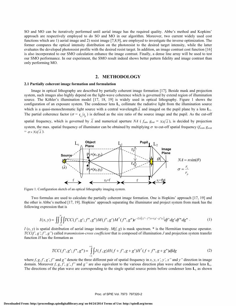
Image in optical lithography are described by partially coherent image formation [17]. Beside mask and projection system, such images also highly depend on the light-wave coherence which is governed by extend region of illumination source. The Köhler’s illumination model [17, 18, 19] is widely used in optical lithography. Figure 1 shows the configuration of an exposure system. The condenser lens Lc collimate the radiative light from the illumination source which is a quasi-monochromatic light source with a central wavelength λ and imaged on the pupil plane by a lens L1. The partial coherence factor (σ = ps rr ) is defined as the size ratio of the source image and the pupil. As the cut-off

spatial frequency, which is governed by λ and numerical aperture NA ( fcut, gcut = λNA ), is decided by projection system, the max. spatial frequency of illuminator can be obtained by multiplying σ to cut-off spatial frequency (fscut, gscut = λσ NA× ).

Figure 1. Configuration sketch of an optical lithography imaging system. Two formulas are used to calculate the partially coherent image formation. One is Hopkins’ approach [17, 19] and the other is Abbe’s method [17, 19]. Hopkins’ approach separating the illuminator and project system from mask has the following expression that is

[ ]∫∫ ∫ ∫ −+−−∞

∞−

= ""'')","()','()",";','(),( ")'(")'(2* dgdfdgdfegfMgfMgfgfTCCyxI yggxffi π . (1)

I (x, y) is spatial distribution of aerial image intensity. M(f, g) is mask spectrum. * is the Hermitian transpose operator. TCC(f’, g’; f”, g”) called transmission-cross coefficient that is composed of illumination J and projection system transfer function H has the formation as

∫ ∫+∞

∞−

++++= dfdgggffHggffHgfJgfgfTCC )","()','(),()",";','( * (2)

where f, g, f’, g’, f” and g” denote the three different pair of spatial frequency in x, y, x’, y’, x” and y” direction in image domain. Moreover f, g, f’, g’, f” and g” are also equivalent to the various direction plan wave after condenser lens Lc. The directions of the plan wave are corresponding to the single spatial source points before condenser lens Lc as shown

P1=(x1,y1)

P2=(x2,y2)

Image Plane

Lc

z0=f f zi=fM f

)(λ

Pupil Object Plane L2L1

Source

rs

rp

p

s

rrnNA

=

=

σ

θ )sin((θ



in left side of figure 1. Hence J(f, g) can be viewed as the spatial frequency response of spatial coherence in image domain and source configuration in source domain. To reduce the calculation complexity, TCC can be decomposed into sum of eigen functions by applying singular value decomposition (SVD) [20, 21]. Thus the Eq. (2) can be adapted as

∑∞

=

ΦΦ=1

* )","()','()",";','(q

qqq gfgfgfgfTCC κ (3)

where κq and Φq are q’th eigenvalue and eigen function of TCC. Substituting Eq. (3) into Eq. (1) and performing inverse fourier transform the equation can be rewritten to spatial position expression via Eq. (4) and (5) that is ),(),(),( yxmyxyxE qq ⊗= φ , (4)

∑=

=Q

qqq yxEyxI

1

2),(),( κ , (5)

where φq(x, y) and m(x, y) are the spatial distribution of Φ q(f, g) and M(f, g) respectively. Eq(x, y) is q’th electric field constructed by a convolution of the coherent kernel φq(x, y). ⊗ and | ⋅ | are the convolution and absolute operator respectively. Because the eigenvalue κq is rapidly decay with increasing q, only Q eigen functions are required. Therefore the calculation complexity decreases from n6 to Q×n4 as m, H ∈ℜn×n. Furthermore Eq. (4) and (5) shows that the mask is stand-alone during image computation. Due to this property, Hopkins’ method is appropriate to simulate the corrected image as performing mask correction. On the contrary, Abbe’s method apart the source effect from image formulation which is

[ ]∫ ∫ ∫ ∫∞

∞−

∞

∞−

+−⎥⎦

⎤⎢⎣

⎡++= dfdgdgdfegfMggffHgfJyxI ygxfi 2''2 '')','()','(),(),( π . (6)

The bracket in Eq. (6) denotes the point source image of source point in (f, g) location. Eq. (6) also shows that Abbe’s method superposes all point source images to obtain the final image of mask. According to this nature, Abbe’s method, where all point source images can be pre-calculated and cached for enhancing the computing, is the favorite image simulation method while optimizing source. For convenient we introduce coefficient ICC, which is the abbreviation of illumination-cross coefficient, to express the contents in bracket of Eq. (6) as

[ ] 2''2 '')','()','(),;,( ∫ ∫∞

∞−

+−++= dgdfegfMggffHgfyxICC ygxfi π . (7)

Furthermore as the optical projection system is a band-limited system, H(f, g) can be presented as a low-pass filter of spatial frequency in image domain that is

⎪⎩

⎪⎨⎧ ≤+=

otherwiseNAgfgfH

,0,1),(

22 λ . (8)

In like manner, J(f, g) can be expressed as

⎪⎩

⎪⎨⎧ ≤+=

otherwiseNAgfgfJgfJ

,0),,(),(

22 λσ , (9)

where λNA is equal to cut-off spatial frequency and λσNA is the max. spatial working region of source in source domain which is relative to the spatial frequency space of image domain.



2.2 Source and mask optimization (SMO)

In this section, we describe the formulation of the objective functions and the computational flow of the SMO by gradient descent algorithm. Three functions are considered in this work: 1) the aerial image, 2) the resist image, and 3) the aerial image contrast. The aerial image represents the optical intensity distribution formed by the projection system on the coated wafer. The resist image corresponds to the resist profile after removing the exposed resist. Finally, the aerial image contrast is highly related to the depth of focus (DOF), and hence determines the process window. For digital computation mask m, aerial image I, coherent kernel φq, electric field Eq, and source J will be sampled to matrix form where m, I, φq, Eq ∈Rn×n and J ∈Rm×m. Moreover to validate the matrix operation, ICC will be pre-calculated and stored as 2D matrix written by ICC where ICC ∈

22 mnR × . Every column of ICC stores the relative source point image of J which is converted to 1D vector via S operator [21] while calculate the aerial image by Abbe’s method. Then the final 1D aerial image is recovered to 2D matrix vis S-1 operator. The operation of S and S-1 can be shown as

12

1

××

⎯⎯←⎯→⎯

−

n

S

Snn RR . (10)

Therefore the aerial image calculated by Abbe’s method can be expressed by Eq. (10) that is ))((1 JSSI ICC−= . (11) Moreover we assume that the optical system is aberration free, so the electric field E is real in nominal condition. Therefore the absolute operator | ⋅ | in Eq. (5) can be left out and the aerial image formulated by Hopkins’ approach can be re-written as

∑=

=Q

qqq EI

1

(κ ⊙ )qE , (12)

where ⊙ is the element-by-element multiplication operator. The aerial image represents the distribution of optical intensity on the wafer, which corresponds to the exposure condition of a photoresist. Some photoresist models employ a Constant Threshold Resist (CTR) [22], where the developed resist profile can then be described by a sigmoid transformation of the aerial image, [8, 9] that is,

)(1

1)(rtIae

IT −−+= . (13)

In Eq. (13), the parameter a describes the sensitivity of the photoresist reacting with the light, which depicts the slope of sidewall profiles, and tr is the parameter of the constant threshold level. Here, the value is set to 0.3. In optical microlithography, the aerial image contrast plays an important role in the development of photoresist, which is directly related to the number of molecular chemical-bonds that are broken or still linked after exposing. As the image intensity difference between the exposed and unexposed regions is desired to be as large as possible, increasing the image contrast can mitigate patterning damages when removing the resist. The image contrast can be express by using a linear differential operator [16], defined as the following:

yyIx

xIIT ˆˆ

∂∂

+∂∂

=∇ , (14)



where T∇ is the differential operator to evaluate the aerial image contrast. Due to the discrete nature of the mask, the differential operator x∂∂ and y∂∂ is approximated by numerical differences. Therefore the operators can be represented in a matrix form D [16] and Eq. (14) re-written into Eq. (15): yIDxDII T

T ˆ)(ˆ)( +=∇ , (15) where D ∈Rn×n. In Eq. (15), DI performs the operation that calculates the difference in the row direction, and IDT computes the column difference. As a result, the three objective functions that evaluate the differences between the desired and the calculated profiles can be expressed as in Eq. (16), Eq. (17) and Eq. (18), respectively: 2IIF tI −= , (16)

( ) ( ) 2ITITF tR −= , (17)

( ) ( )22

IIy

IIx

F ttC −∂∂

+−∂∂

= , (18)

Here, FI, FR and FC represent the costs for the aerial image, resist image, and aerial image contrast, respectively. It is the desired target image which is parameterized by wavefront expansion technique previously developed by us [16, 23]. The norm 2

⋅ denotes the square of Euclidean distance which denotes the inner product of the same vector. Moreover, we can

further combine the components into a total cost function, F by assigning three weighting coefficients, Iγ , Rγ , and Cγ to the aerial image, resist image, and aerial image contrast, respectively. The final expression is then as follows: CCRII FFFF γγγ ++= R . (19) The goal of SMO is to find the optimal source Ĵ and mask m̂ that minimizes a given constraint and therefore can be expressed as in Eq. (20): ),()ˆ,ˆ(

),(mJFmJ

mJargmin= . (20)

A gradient-search method used to calculate Ĵ and m̂ is explained next. Since the gradient operation calculates the derivatives of the mask, the discrete binary mask described by m, must be first parameterized by a continuous variable θ in order to obtain an analyzable form. Here, a sinusoidal transformation is employed to convert a binary drawn mask in to a continuous grey-level mask [8]:

2

)cos(1 θ+=m . (21)

We note that π≤≤∈ × θθ 0,nnR . The converted mask then allows a continuous optical transmission value between zero

and unity with θ varying between zero and π. The cost function gradient of source FJ∇ and mask Fm∇ can be derived as shown in Eq. (22) and (23) CJCRJIJIJ FFFF ∇+∇+∇=∇ γγγ R , (22) CmCRmImIm FFFF ∇+∇+∇=∇ γγγ R . (23)



<kmnWpE

The explicit expressions of the objective functions of source gradient for the aerial image, resist image and image contrast are listed in following that are =∇ IJ F ( )( )ICCT12 IISS t −− − , (24)

=∇ RJ F ( ( ))()((2 1 ITITSS t −− − ⊙ ))(1(( ITa − ⊙ ) )ICCT)(IT , (25)

=∇ CJ F ( )( )ICCT1 ))(())((2 DDIIIIDDSS Ttt

T −+−− − . (26) For mask gradient, the explicit expressions are

=∇ IFθ ( ( )[∑=

−−Q

qtq II

12κ ⊙ ] )flip

qqE φ⊗2 ⊙ ⎟⎠⎞

⎜⎝⎛−

2)sin(θ , (27)

=∇ RFθ ∑ −−Q

qtq ITIT ))()((2[( κ ⊙ ))(1(( ITa − ⊙ ))(IT ⊙ )]2 flip

qqE φ⊗ ⊙ ⎟⎠⎞

⎜⎝⎛−

2)sin(θ , (28)

=∇ CFθ ∑=

−+−−Q

q

Ttt

Tq DDIIIIDD

1)))((2))(((2[( κ ⊙ )]2 flip

qqE φ⊗ ⊙ ⎟⎠⎞

⎜⎝⎛−

2)sin(θ , (29)

where ⊙ is the element-by-element multiplication operator and ⊗ is the convolution operator. Furthermore, flip

qφ is the

up-down and left-right flip of qφ , i.e. =),( jiflipqφ )1,1( +−+− jninqφ where i, j are integers and ∈[1, N].

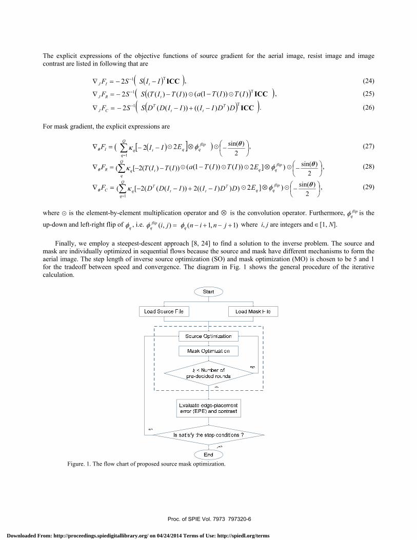
Finally, we employ a steepest-descent approach [8, 24] to find a solution to the inverse problem. The source and mask are individually optimized in sequential flows because the source and mask have different mechanisms to form the aerial image. The step length of inverse source optimization (SO) and mask optimization (MO) is chosen to be 5 and 1 for the tradeoff between speed and convergence. The diagram in Fig. 1 shows the general procedure of the iterative calculation.

Figure. 1. The flow chart of proposed source mask optimization.



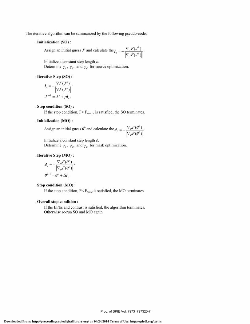
The iterative algorithm can be summarized by the following pseudo-code:

．Initialization (SO) :

Assign an initial guess J0 and calculate the)()(

0

0

0 JFJF

J

J

∇∇

−=l .

Initialize a constant step length ρ. Determine Iγ , Rγ , and Cγ for source optimization.

．Iterative Step (SO) :

)()(

u

u

u JFJF

∇∇

−=l .

uuu JJ lρ+=+1 .

．Stop condition (SO) : If the stop condition, F< Fsource is satisfied, the SO terminates.

．Initialization (MO) :

Assign an initial guess θ0 and calculate the)()(

0

0

0 θθd

θ

θ

FF

∇∇

−= .

Initialize a constant step length δ. Determine Iγ , Rγ , and Cγ for mask optimization.

．Iterative Step (MO) :

)()(

v

v

v FFθθd

θ

θ

∇∇

−= .

vvv dθθ δ+=+1 .

．Stop condition (MO) : If the stop condition, F< Fmask is satisfied, the MO terminates. ．Overall stop condition : If the EPEs and contrast is satisfied, the algorithm terminates. Otherwise re-run SO and MO again.



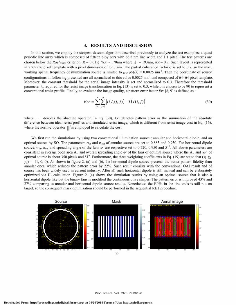
3. RESULTS AND DISCUSSION In this section, we employ the steepest-descent algorithm described previously to analyze the test examples: a quasi periodic line array which is composed of fifteen ploy bars with 86.2 nm line width and 1:1 pitch. The test patterns are chosen below the Rayleigh criterion: R = 0.61 λ /NA ~ 170nm where λ = 193nm, NA = 0.7. Such layout is represented in 256×256 pixel template with a pixel dimension of 12.3 nm. The partial coherence factor σ is set to 0.7, so the max. working spatial frequency of illumination source is limited to λσ NA× = 0.0025 nm-1. Then the coordinate of source configurations in following presented are all normalized to this value 0.0025 nm-1 and composed of 64×64 pixel template. Moreover, the constant threshold for the aerial image intensity is set and normalized to 0.3. Therefore the threshold parameter tr, required for the resist image transformation in Eq. (13) is set to 0.3, while a is chosen to be 90 to represent a conventional resist profile. Finally, to evaluate the image quality, a pattern error factor Err [8, 9] is defined as :

( ) ( )∑∑= =

−=n

i

n

jt jiITjiITErr

1 1),(),( (30)

where | ⋅ | denotes the absolute operator. In Eq. (30), Err denotes pattern error as the summation of the absolute difference between ideal resist profiles and simulated resist image, which is different from resist image cost in Eq. (16). where the norm-2 operator 2

⋅ is employed to calculate the cost. We first run the simulations by using two conventional illumination source : annular and horizontal dipole, and an optimal source by SO. The parameters σin and σout of annular source are set to 0.885 and 0.950. For horizontal dipole source, σin, σout and spreading angle of the fans ϕ are respective set to 0.720, 0.950 and 510. All above parameters are consistent in average open area A’

s and overall spreading angle ϕ’ of the fans of optimal source where the A’s and ϕ’ of

optimal source is about 350 pixels and 510. Furthermore, the three weighting coefficients in Eq. (19) are set to that (γI, γR, γC) = (1, 0, 0). As shown in figure 2. (a) and (b), the horizontal dipole source presents the better pattern fidelity than annular ones, which reduces the pattern error by 22%. Such result consists with the conventional OAI result and of course has been widely used in current industry. After all such horizontal dipole is still manual and can be elaborately optimized via IL calculation. Figure 2. (c) shows the simulation results by using an optimal source that is also a horizontal dipole like but the binary fans is modified the continuous olive shapes. The pattern error is improved 43% and 27% comparing to annular and horizontal dipole source results. Nonetheless the EPEs in the line ends is still not on target, so the consequent mask optimization should be performed in the sequential RET procedure.

-1 -0.8 -0.6 -0.4 -0.2 0 0.2 0.4 0.6 0.8 1

-1

-0.8

-0.6

-0.4

-0.2

0

0.2

0.4

0.6

0.8

1

00

300

600

900

1200

1500

1800

2100

2400

2700

3000

3300

0.2

0.4

0.6

0.8

1

0.03

0.19

0.34

0.50

0.66

0.81

0.97

50 100 150 200 250

50

100

150

200

250

0.09

0.25

0.41

0.56

0.72

0.88

Pattern error = 4455.9472

50 100 150 200 250

50

100

150

200

250

0.16

0.31

0.47

0.63

0.78

0.94

Source Mask Aerial image

(a)



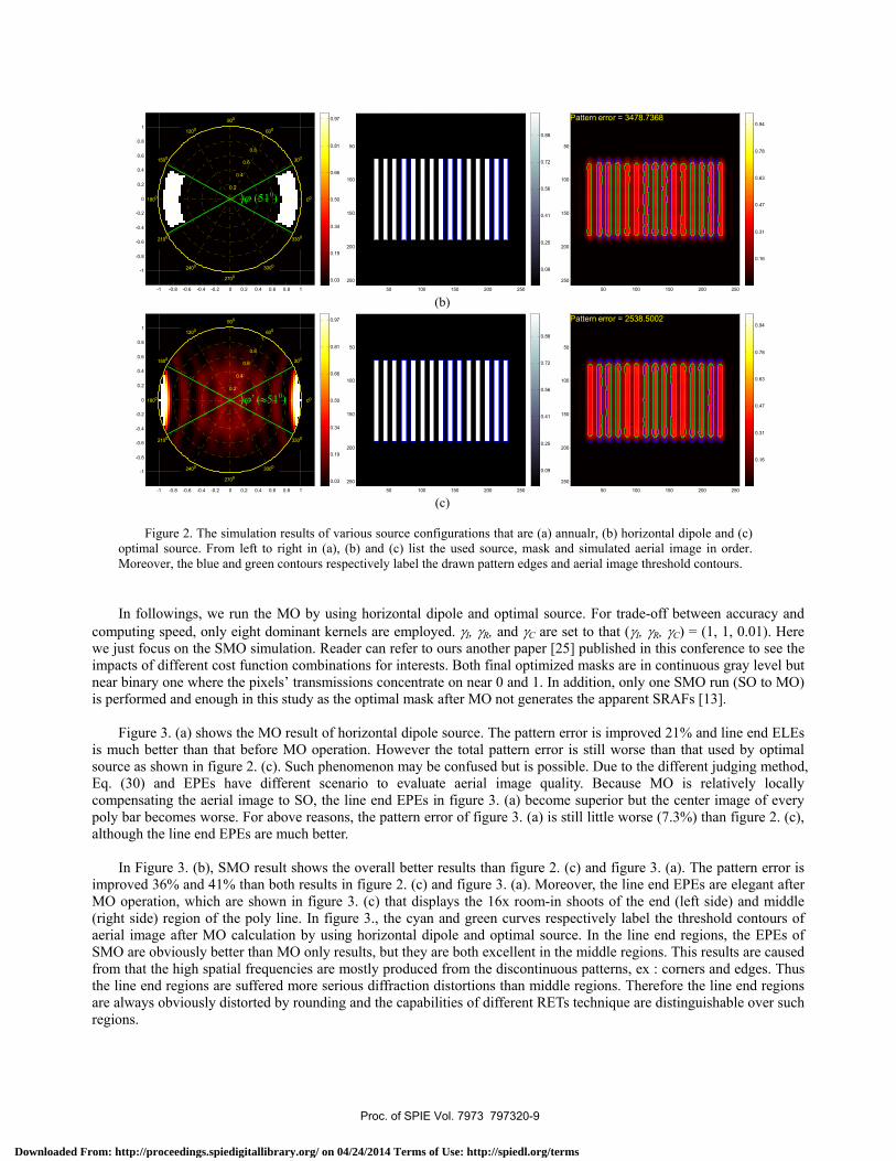
Figure 2. The simulation results of various source configurations that are (a) annualr, (b) horizontal dipole and (c) optimal source. From left to right in (a), (b) and (c) list the used source, mask and simulated aerial image in order. Moreover, the blue and green contours respectively label the drawn pattern edges and aerial image threshold contours.

In followings, we run the MO by using horizontal dipole and optimal source. For trade-off between accuracy and computing speed, only eight dominant kernels are employed. γI, γR, and γC are set to that (γI, γR, γC) = (1, 1, 0.01). Here we just focus on the SMO simulation. Reader can refer to ours another paper [25] published in this conference to see the impacts of different cost function combinations for interests. Both final optimized masks are in continuous gray level but near binary one where the pixels’ transmissions concentrate on near 0 and 1. In addition, only one SMO run (SO to MO) is performed and enough in this study as the optimal mask after MO not generates the apparent SRAFs [13]. Figure 3. (a) shows the MO result of horizontal dipole source. The pattern error is improved 21% and line end ELEs is much better than that before MO operation. However the total pattern error is still worse than that used by optimal source as shown in figure 2. (c). Such phenomenon may be confused but is possible. Due to the different judging method, Eq. (30) and EPEs have different scenario to evaluate aerial image quality. Because MO is relatively locally compensating the aerial image to SO, the line end EPEs in figure 3. (a) become superior but the center image of every poly bar becomes worse. For above reasons, the pattern error of figure 3. (a) is still little worse (7.3%) than figure 2. (c), although the line end EPEs are much better. In Figure 3. (b), SMO result shows the overall better results than figure 2. (c) and figure 3. (a). The pattern error is improved 36% and 41% than both results in figure 2. (c) and figure 3. (a). Moreover, the line end EPEs are elegant after MO operation, which are shown in figure 3. (c) that displays the 16x room-in shoots of the end (left side) and middle (right side) region of the poly line. In figure 3., the cyan and green curves respectively label the threshold contours of aerial image after MO calculation by using horizontal dipole and optimal source. In the line end regions, the EPEs of SMO are obviously better than MO only results, but they are both excellent in the middle regions. This results are caused from that the high spatial frequencies are mostly produced from the discontinuous patterns, ex : corners and edges. Thus the line end regions are suffered more serious diffraction distortions than middle regions. Therefore the line end regions are always obviously distorted by rounding and the capabilities of different RETs technique are distinguishable over such regions.

-1 -0.8 -0.6 -0.4 -0.2 0 0.2 0.4 0.6 0.8 1

-1

-0.8

-0.6

-0.4

-0.2

0

0.2

0.4

0.6

0.8

1

00

300

600

900

1200

1500

1800

2100

2400

2700

3000

3300

0.2

0.4

0.6

0.8

1

0.03

0.19

0.34

0.50

0.66

0.81

0.97

50 100 150 200 250

50

100

150

200

250

0.09

0.25

0.41

0.56

0.72

0.88


50 100 150 200 250

50

100

150

200

250

0.16

0.31

0.47

0.63

0.78

0.94

)ϕ’ (≈510)

(b)

(c)

-1 -0.8 -0.6 -0.4 -0.2 0 0.2 0.4 0.6 0.8 1

-1

-0.8

-0.6

-0.4

-0.2

0

0.2

0.4

0.6

0.8

1

00

300

600

900

1200

1500

1800

2100

2400

2700

3000

3300

0.2

0.4

0.6

0.8

1

0.03

0.19

0.34

0.50

0.66

0.81

0.97

50 100 150 200 250

50

100

150

200

250

0.09

0.25

0.41

0.56

0.72

0.88


50 100 150 200 250

50

100

150

200

250

0.16

0.31

0.47

0.63

0.78

0.94

)ϕ (510)



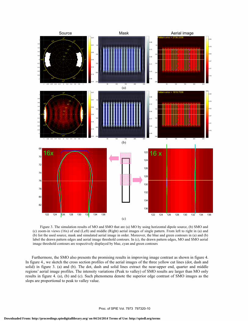
Figure 3. The simulation results of MO and SMO that are (a) MO by using horizontal dipole source, (b) SMO and (c) zoom-in views (16x) of end (Left) and middle (Right) aerial images of single pattern. From left to right in (a) and (b) list the used source, mask and simulated aerial image in order. Moreover, the blue and green contours in (a) and (b) label the drawn pattern edges and aerial image threshold contours. In (c), the drawn pattern edges, MO and SMO aerial image threshold contours are respectively displayed by blue, cyan and green contours

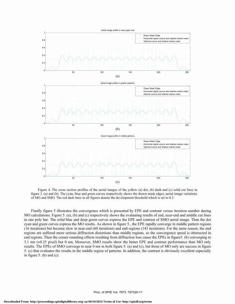
Furthermore, the SMO also presents the promising results in improving image contrast as shown in figure 4. In figure 4., we sketch the cross section profiles of the aerial images of the three yellow cut lines (dot, dash and solid) in figure 3. (a) and (b). The dot, dash and solid lines extract the near-upper end, quarter and middle regions’ aerial image profiles. The intensity variations (Peak to valley) of SMO results are larger than MO only results in figure 4. (a), (b) and (c). Such phenomena denote the superior edge contrast of SMO images as the slops are proportional to peak to valley value.

Source Mask Aerial image

(a)

(b)

(c)122 124 126 128 130 132 134 136

68

70

72

74

76

78

80

82

16x

122 124 126 128 130 132 134 136

122

124

126

128

130

132

134

136

16 x

-1 -0.8 -0.6 -0.4 -0.2 0 0.2 0.4 0.6 0.8 1

-1

-0.8

-0.6

-0.4

-0.2

0

0.2

0.4

0.6

0.8

1

00

300

600

900

1200

1500

1800

2100

2400

2700

3000

3300

0.2

0.4

0.6

0.8

1

0.03

0.19

0.34

0.50

0.66

0.81

0.97

50 100 150 200 250

50

100

150

200

250

0.09

0.25

0.41

0.56

0.72

0.88


50 100 150 200 250

50

100

150

200

250

0.16

0.31

0.47

0.63

0.78

0.94

-1 -0.8 -0.6 -0.4 -0.2 0 0.2 0.4 0.6 0.8 1

-1

-0.8

-0.6

-0.4

-0.2

0

0.2

0.4

0.6

0.8

1

00

300

600

900

1200

1500

1800

2100

2400

2700

3000

3300

0.2

0.4

0.6

0.8

1

0.03

0.19

0.34

0.50

0.66

0.81

0.97

50 100 150 200 250

50

100

150

200

250

0.09

0.25

0.41

0.56

0.72

0.88


50 100 150 200 250

50

100

150

200

250

0.16

0.31

0.47

0.63

0.78

0.94

Proc. of SPIE Vol. 7973 797320-10


50 100 150 200 2500

0.2

0.4

0.6

0.8

1Aerial image profile in near-upper end

Drawn Mask EdgeHorizontal dipole source and relative inverse maskOptimal source and relative inverse mask

(a)

50 100 150 200 2500

0.2

0.4

0.6

0.8

1Aerial image profile in quarter patterns


(b)

50 100 150 200 2500

0.2

0.4

0.6

0.8

1Aerial image profile in middle patterns


(c)

Figure 4. The cross section profiles of the aerial images of the yellow (a) dot, (b) dash and (c) solid cut lines in

figure 3. (a) and (b). The cyan, blue and green curves respectively shows the drawn mask edges, aerial image variations of MO and SMO. The red dash lines in all figures denote the development threshold which is set to 0.3.

Finally figure 5 illustrates the convergence which is presented by EPE and contrast versus iteration number during MO calculations. Figure 5. (a), (b) and (c) respectively shows the evaluating results of end, near-end and middle cut lines in one poly bar. The solid blue and deep green curves express the EPE and contrast of SMO aerial image. Then the dot cyan and green curves express the MO results. As shown in figure 5., the EPE rapidly converge in middle pattern regions (16 iterations) but become slow in near-end (60 iterations) and end regions (143 iterations). For the same reason, the end regions are suffered more serious diffraction distortions than middle regions, so the convergence speed is obstructed in end regions. Then the corner rounding effects resulting from diffraction loss cause the EPEs in figure5. (b) converging to 3.1 nm (≈0.25 pixel) but 0 nm. Moreover, SMO results show the better EPE and contrast performance than MO only results. The EPEs of SMO converge to near 0 nm in both figure 5. (a) and (c), but those of MO only are success in figure 5. (c) that evaluates the results in the middle region of patterns. In addition, the contrast is obviously excellent especially in figure 5. (b) and (c).

Proc. of SPIE Vol. 7973 797320-11


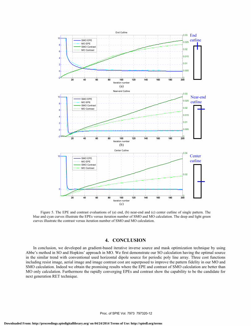
Figure 5. The EPE and contrast evaluations of (a) end, (b) near-end and (c) center cutline of single pattern. The blue and cyan curves illustrate the EPEs versus iteration number of SMO and MO calculation. The deep and light green curves illustrate the contrast versus iteration number of SMO and MO calculation.

4. CONCLUSION In conclusion, we developed an gradient-based iterative inverse source and mask optimization technique by using Abbe’s method in SO and Hopkins’ approach in MO. We first demonstrate our SO calculation having the optimal source in the similar trend with conventional used horizontal dipole source for periodic poly line array. Three cost functions including resist image, aerial image and image contrast cost are superposed to improve the pattern fidelity in our MO and SMO calculation. Indeed we obtain the promising results where the EPE and contrast of SMO calculation are better than MO only calculation. Furthermore the rapidly converging EPEs and contrast show the capability to be the candidate for next generation RET technique.

(a)

(b)

(c)

20 40 60 80 100 120 140 160 180 200-2

0

2

4

6

8

10

Iteration number

End Cutline

20 40 60 80 100 120 140 160 180 2000

0.005

0.01

0.015

0.02

0.025

0.03

SMO EPEMO EPESMO ContrastMO Contrast

20 40 60 80 100 120 140 160 180 200-2

0

2

4

6

8

10

Iteration number

Near-end Cutline

20 40 60 80 100 120 140 160 180 2000

0.005

0.01

0.015

0.02

0.025

0.03


20 40 60 80 100 120 140 160 180 200

0

10

Iteration number

Center Cutline

20 40 60 80 100 120 140 160 180 2000

0.02

0.04


End cutline

Near-end cutline

Center cutline

Proc. of SPIE Vol. 7973 797320-12


REFERENCES

[1] D. S. Abrams and L. Pang, “Fast inverse lithography technology,” Proc. SPIE 6154, 534-542 (2006). [2] C. Hung, B. Zhang, E. Guo, L. Pang, Y. Liu, K. Wang, and G. Dai, “Pushing the lithography limit: Applying

inverse lithography technology (ILT) at the 65nm generation,” Proc. SPIE 6154, 61541M (2006). [3] L. Pang, Y. Liu, and D. Abrams, “Inverse lithography technology (ILT): What is the impact to the photomask

industry?” Proc. SPIE 6283, 62830X (2006). [4] S. Sherif, B. Saleh, and R. Leone, “Binary image synthesis using mixed linear integer programming,” IEEE

Trans. Image Process. Papers 4, 1252–1257 (1995). [5] K. Nashold and B. Saleh, “Image construction through diffraction-limited high-contrast imaging systems: An

iterative approach,” J. Opt. Soc. Am. A Papers 2, 635–643 (1985). [6] B. Saleh and S. Sayegh, “Reductions of errors of microphotographic reproductions by optical corrections of

original masks,” Opt. Eng. Papers 20, 781–784 (1981). [7] Yuri Granik, “Fast pixel-based mask optimization for inverse lithography,” J. Microlith., Microfab., Microsyst.

Papers 5, 043002 (2006). [8] A. Poonawala and P. Milanfar, “Mask design for optical microlithography — An inverse imaging problem,”

IEEE Trans. Image Process. Papers 16, 774–788 (2007). [9] Xu Ma and G. R. Arce, “Generalized inverse lithography methods for phase-shifting mask design,” Optics

Express Papers 15, 15066-15079 (2007). [10] Stanley H. Chan, Alfred K.Wong, and Edmund Y. Lam, “Initialization for robust inverse synthesis of phase-

shifting masks in optical projection lithography,” Optics Express Papers 16, 14746-14760 (2008). [11] Stephen Hsu, Zhipan Li, Luoqi Chen, Keith Gronlund, Hua-yu Liu, and Robert Socha, “Source-mask co-

optimization: optimize design for imaging and impact of source complexity on lithography performance,” Proc. SPIE 7520, 75200D (2009).

[12] Amir Sagiv, Jo Finders, Robert Kazinczi, Andre Engelen, Frank Duray, Ingrid Minnaert-Janssen, Shmoolik Mangan, Dror Kasimov, and Ilan Englard, “Aerial imaging for source mask optimization: mask and illumination qualification,” Proc. SPIE 7488, 74880Z (2009).

[13] Linyong Pang, Peter Hu, Danping Peng, Dongxue Chen, Tom Cecil, Lin He, Guangming Xiao, Vikram Tolani, Thuc Dam, Ki-Ho Baik, and Bob Gleason, “Source mask optimization (SMO) at full chip scale using inverse lithography technology (ILT) based on level set methods,” Proc. SPIE 7520, 75200X (2009).

[14] Jason Hsih-Chie Chang, Charlie Chung-Ping Chen, and Lawrence S. Melvin III, “Abbe-PCA-SMO: microlithography source and mask optimization based on Abbe-PCA,” Proc. SPIE 7640, 764026 (2010).

[15] Ma, Xu and Arce, Gonzalo R, “Pixel-based simultaneous source and mask optimization for resolution enhancement in optical lithography,” Optics Express Papers 17, 5783-5793 (2009).

[16] Yu, Jue-Chin and Yu, Peichen, “Impacts of cost functions on inverse lithography patterning ,” Optics Express Papers 18, 23331-23342 (2010)

[17] M. Born and E. Wolf, [Principles of Optics], 7th(expanded) ed., Cambridge University Press, 598-599 (1999). [18] J. W. Goodman, [Statistical Optics], John Wiley & Sons, New York, 306-307 (1985). [19] A. K. Wong, [Optical Imaging in Projection Microlithography], SPIE Press, Bellingham Washington, 157-159

(2005). [20] Steven J. Leon, [Linear Algebra with applications], 6th ed., Prentice-Hall, 367-380 (2002). [21] N. B. Cobb, [Fast optical and process proximity correction algorithms for integrated circuit manufacturing],

University of California at Berkeley, Berkely California, 51-60 (1998). [22] W. Huang, C. Lin, C. Kuo, C. Huang, J. Lin, J. Chen, R. Liu, Y. Ku, and B. Lin, “Two threshold resist models

for optical proximity correction,” Proc. SPIE 5377, 1536–1543 (2001). [23] Jue-Chin Yu, Peichen Yu, and Hsueh-Yung Chao, “Model-based sub-resolution assist features using an inverse

lithography method,” Proc. SPIE 7140, 714014 (2008). [24] M. Minoux, [Mathematical programming theory and algorithms], John Wiley & Sons, New York, 84-89 (1986). [25] Jue-Chin Yu and Peichen Yu, “Choosing objective functions for inverse lithography patterning,” presented at

the SPIE Advanced Lithography, San Jose, California, USA, 27 Feb.- 3 Mar. 2011.

Proc. of SPIE Vol. 7973 797320-13


Documents

Gradient-Based Fast Source Mask Optimization (SMO) Fast Source Mask Optimization (SMO) Jue-Chin Yu and Peichen Yu Department of Photonics and Institute of Electro-Optical Engineering,