Gradient Art: Creation and Vectorization - Inria 6 Gradient Art: Creation and Vectorization Pascal Barla and Adrien Bousseau Abstract There are two different categories of methods

HAL Id: hal-00760068https://hal.inria.fr/hal-00760068

Submitted on 3 Dec 2012

HAL is a multi-disciplinary open accessarchive for the deposit and dissemination of sci-entific research documents, whether they are pub-lished or not. The documents may come fromteaching and research institutions in France orabroad, or from public or private research centers.

L’archive ouverte pluridisciplinaire HAL, estdestinée au dépôt et à la diffusion de documentsscientifiques de niveau recherche, publiés ou non,émanant des établissements d’enseignement et derecherche français ou étrangers, des laboratoirespublics ou privés.

Gradient Art: Creation and VectorizationPascal Barla, Adrien Bousseau

To cite this version:Pascal Barla, Adrien Bousseau. Gradient Art: Creation and Vectorization. John Colomosse, PaulRosin. Image and Video based Artistic Stylization, Springer, 2012. <hal-00760068>

https://hal.inria.fr/hal-00760068

https://hal.archives-ouvertes.fr

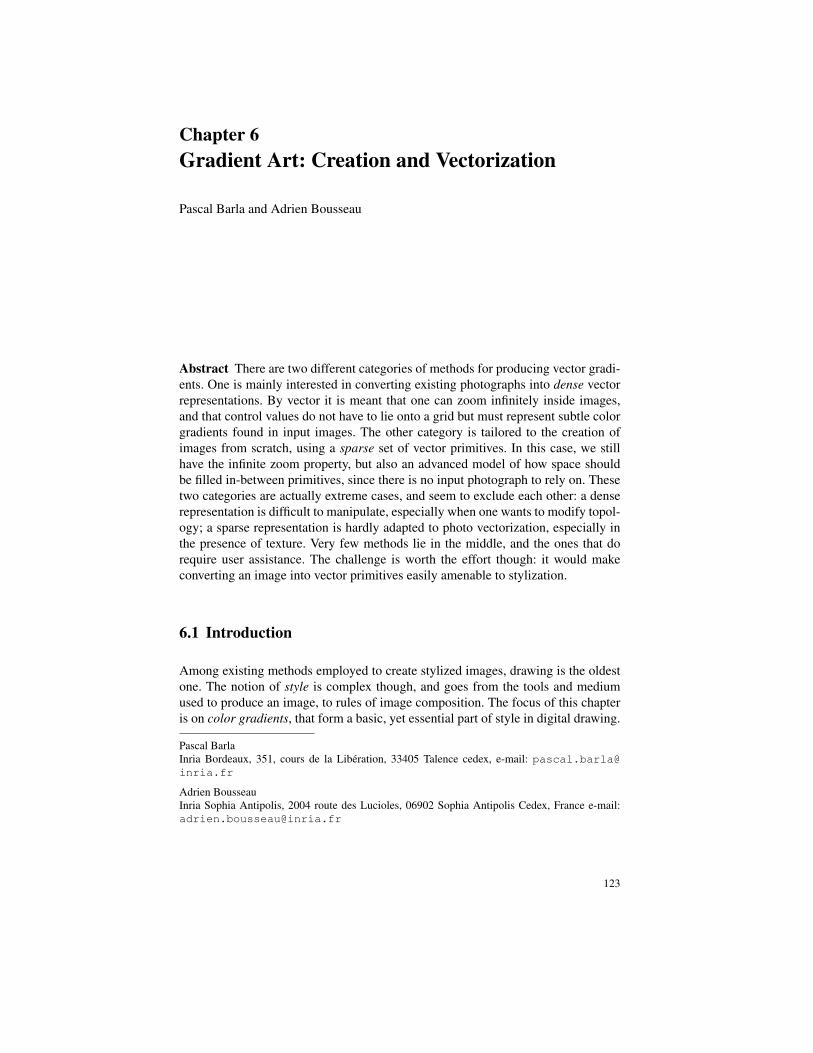
Chapter 6

Gradient Art: Creation and Vectorization

Pascal Barla and Adrien Bousseau

Abstract There are two different categories of methods for producing vector gradi-

ents. One is mainly interested in converting existing photographs into dense vector

representations. By vector it is meant that one can zoom infinitely inside images,

and that control values do not have to lie onto a grid but must represent subtle color

gradients found in input images. The other category is tailored to the creation of

images from scratch, using a sparse set of vector primitives. In this case, we still

have the infinite zoom property, but also an advanced model of how space should

be filled in-between primitives, since there is no input photograph to rely on. These

two categories are actually extreme cases, and seem to exclude each other: a dense

representation is difficult to manipulate, especially when one wants to modify topol-

ogy; a sparse representation is hardly adapted to photo vectorization, especially in

the presence of texture. Very few methods lie in the middle, and the ones that do

require user assistance. The challenge is worth the effort though: it would make

converting an image into vector primitives easily amenable to stylization.

6.1 Introduction

Among existing methods employed to create stylized images, drawing is the oldest

one. The notion of style is complex though, and goes from the tools and medium

used to produce an image, to rules of image composition. The focus of this chapter

is on color gradients, that form a basic, yet essential part of style in digital drawing.

Pascal Barla

Inria Bordeaux, 351, cours de la Libération, 33405 Talence cedex, e-mail: pascal.barla@

inria.fr

Adrien Bousseau

Inria Sophia Antipolis, 2004 route des Lucioles, 06902 Sophia Antipolis Cedex, France e-mail:

[email protected]

123

[email protected]

[email protected]

[email protected]

124 Pascal Barla and Adrien Bousseau

(a) Fernand Leger (b) Nash Ambassador

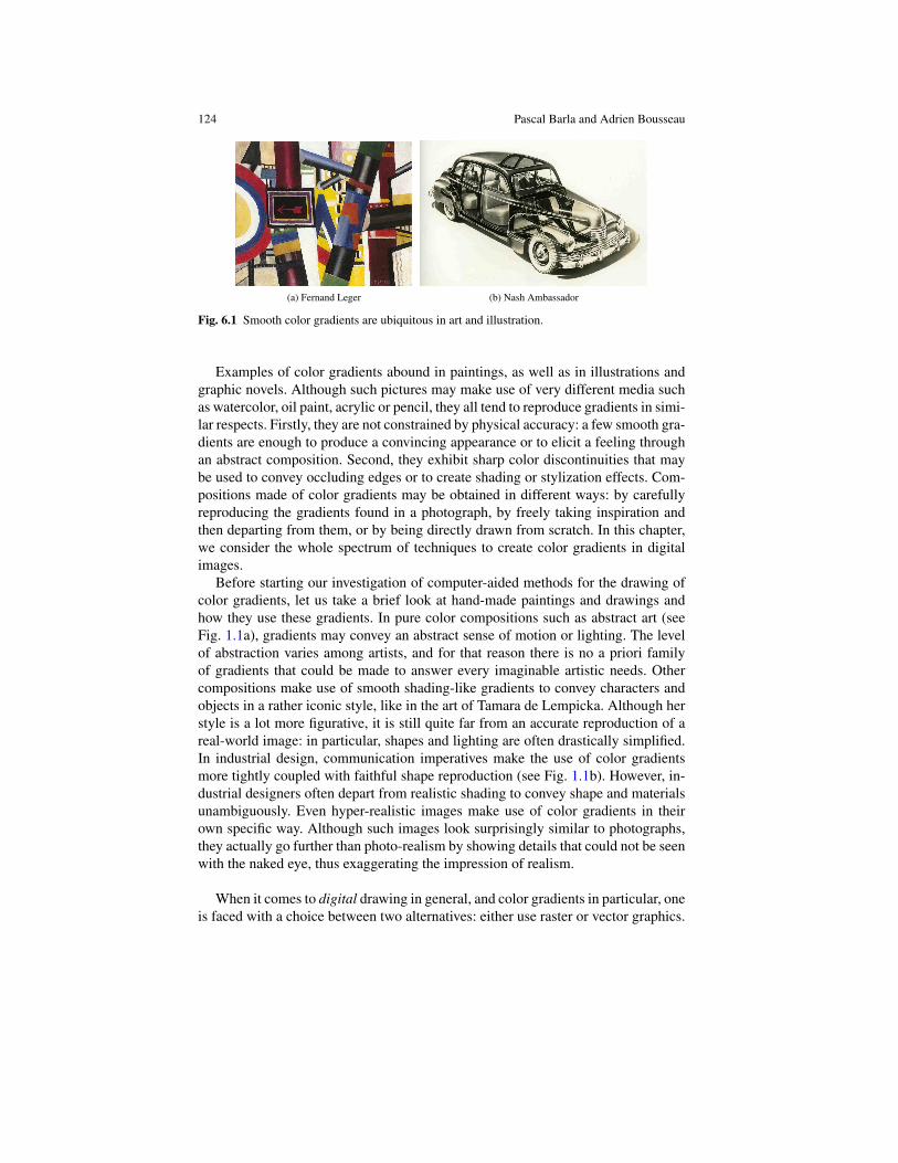
Fig. 6.1 Smooth color gradients are ubiquitous in art and illustration.

Examples of color gradients abound in paintings, as well as in illustrations and

graphic novels. Although such pictures may make use of very different media such

as watercolor, oil paint, acrylic or pencil, they all tend to reproduce gradients in simi-

lar respects. Firstly, they are not constrained by physical accuracy: a few smooth gra-

dients are enough to produce a convincing appearance or to elicit a feeling through

an abstract composition. Second, they exhibit sharp color discontinuities that may

be used to convey occluding edges or to create shading or stylization effects. Com-

positions made of color gradients may be obtained in different ways: by carefully

reproducing the gradients found in a photograph, by freely taking inspiration and

then departing from them, or by being directly drawn from scratch. In this chapter,

we consider the whole spectrum of techniques to create color gradients in digital

images.

Before starting our investigation of computer-aided methods for the drawing of

color gradients, let us take a brief look at hand-made paintings and drawings and

how they use these gradients. In pure color compositions such as abstract art (see

Fig. 1.1a), gradients may convey an abstract sense of motion or lighting. The level

of abstraction varies among artists, and for that reason there is no a priori family

of gradients that could be made to answer every imaginable artistic needs. Other

compositions make use of smooth shading-like gradients to convey characters and

objects in a rather iconic style, like in the art of Tamara de Lempicka. Although her

style is a lot more figurative, it is still quite far from an accurate reproduction of a

real-world image: in particular, shapes and lighting are often drastically simplified.

In industrial design, communication imperatives make the use of color gradients

more tightly coupled with faithful shape reproduction (see Fig. 1.1b). However, in-

dustrial designers often depart from realistic shading to convey shape and materials

unambiguously. Even hyper-realistic images make use of color gradients in their

own specific way. Although such images look surprisingly similar to photographs,

they actually go further than photo-realism by showing details that could not be seen

with the naked eye, thus exaggerating the impression of realism.

When it comes to digital drawing in general, and color gradients in particular, one

is faced with a choice between two alternatives: either use raster or vector graphics.

6 Gradient Art: Creation and Vectorization 125

Raster graphics solutions such as Adobe Photoshop, Corel Painter or Gimp offer

by design a more direct analogy with traditional, hand-made paintings and drawings:

each drawn brush stroke is recorded in a pixel grid that represents the canvas, and

blended in a variety of ways depending on the choice of tool and medium. Tools may

tightly simulate their real-world counterparts (e.g., [2]), or they might provide novel

types of interactions (e.g., [18]). In both cases though, users create color gradients

by layering multiple strokes. The first issue raised by this layering approach is that

the resulting gradient is not easily editable, and artists usually have to re-paint over

them when a change is required. A second limitation of raster images is their lack

of scalability: the resolution of the pixel grid limits the amount of details that can be

drawn.

Vector graphics, on the other hand, offer a more compact representation, res-

olution independence (allowing scaling of images while retaining sharp edges),

and geometric editability. Vector-based images are more easily animated (through

keyframe animation of their underlying geometric primitives), and more readily

stylized (e.g. through controlled perturbation of geometry). For all of these reasons,

vector-based drawing tools, such as Adobe Illustrator, Corel Draw, and Inkscape,

continue to enjoy great popularity, as do standardized vector representations, such

as Flash and SVG.

However, for all of their benefits, basic vector drawing tools offer limited support

for representing complex color gradients, which are integral to many artistic styles.

In order to better understand these limitations, let us consider the following two

important requirements for any vector-based solution:

1. Accurate manual control should be provided at sharp discontinuities, while a

somewhat more automated control (albeit accurate) is preferable in smooth re-

gions. These different levels of control are necessary because small changes of

sharp color variations are more noticeable, while smooth color variations are

more difficult to draw.

2. Completing a drawing should require as few vector primitives as possible to get

to the intended result. Such sparse representations are necessary to endow artists

with more direct control of entire parts of the image at once, and limit the amount

of user interaction for simple edits.

Basic color gradient tools have huge restrictions regarding both requirements.

In a nutshell, they require many primitives to create even simple images, work

solely with closed contours, and provide only for very simple interior behaviors.

Section 1.2 explains these limitations in detail, and presents the alternative primi-

tives that form the core of this chapter.

Despite considerable improvements in vector-based color gradient primitives, we

must say that as of today, there is no single solution that fulfils the above-mentioned

requirements unequivocally. This is mainly due to the extent to which each method

makes use of a reference raster image. For methods that strive to faithfully convert a

photograph to a vector representation — a process known as vectorization — prim-

itives need to stick as much as possible to underlying color variations (req.1), hence


making it hard to provide holistic editing functionalities (req.2). On the opposite end

of the spectrum, methods that let artists create color gradients from scratch — i.e.,

vector drawing — must at the same time provide control in precise locations (req.1),

and incorporate priors to fill-in smooth regions with few primitives (req.2). These

examples are extreme cases, and a host of intermediate solutions has been proposed

in the literature. This is elaborated in greater depth in Section 1.3.

An ideal solution would reside in a single tool for both vector drawing and image

vectorization: one could start from an image and more or less deviate from it ac-

cording to the intended message conveyed by the picture, in a style either personal

or optimized for legibility for instance. Even if such a method becomes available

one day, there will still be a last important point to consider: with more advanced

conversion and editing capabilities come more complex rendering requirements. To

reach a wide audience, the rendering of vector-based color gradients should be effi-

cient (ideally real-time) and robust (artifact-free). We present in Section 1.4 existing

rendering solutions and compare their merits.

The gradient primitives, construction techniques and rendering algorithms pre-

sented in the following sections have been used for applications outside of color

gradients. One important instance is the (re-)construction of normal and/or depth

images (e.g. [14]), which provide for 3D-like shading capabilities. We refer the in-

terested reader to Sections 12.3.2 to 12.3.3 of this book, where it is shown how

diffusion-based methods in particular have proven useful for a variety of applica-

tions. We have intentionally focused on still 2D graphics; throughout the chapter,

we will also mention vector-based 3D methods, but only in contexts where they are

of interest to 2D color gradients.

6.2 Gradient primitives

We start by describing existing gradient primitives, focusing on how they are created

and manipulated. We distinguish between three families of primitives: elemental

primitives that fill the whole space given a small set of parameters, primitives that

rely on meshes to provide more accurate and dense control, and primitives that rely

on extremal curves and a propagation process to fill-in space between them.

6.2.1 Elemental gradients

Elemental gradients are composed of two ingredients: a parametrization of the plane

R2→ [0,1], and a one-dimensional color gradient [0,1]→ [0,1]4 that assigns a color

and opacity to each parametric value. The types of gradients differ in the way they

define the parametrization from two control points. The most common parametriza-

tions are linear, radial and polar, as shown in Fig. 1.2: a linear gradient produces

constant colors along directions perpendicular to the line defined by the two control


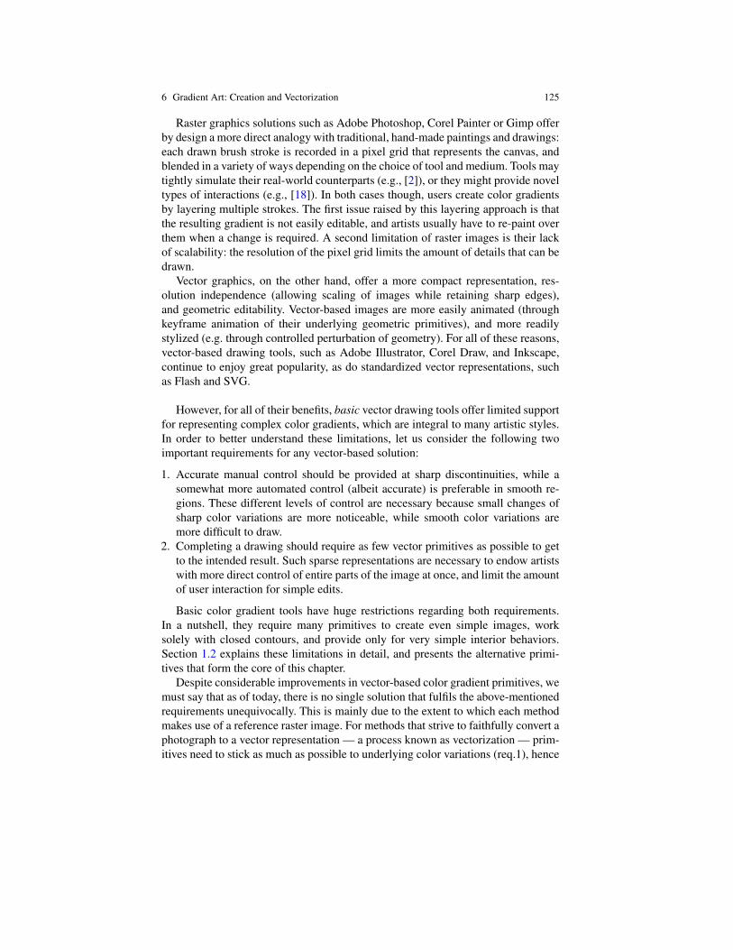
(a) Linear (b) Radial (c) Polar

Fig. 6.2 Examples of elemental gradients and their parameterization and color control points.

points; a radial gradient produces circles of constant colors centered on the first con-

trol point; a polar gradient produces rays of constant colors originating from the first

anchor point. In the last case, the 1D gradient should be periodic to avoid color dis-

continuities. The distance function may be adapted to produce contours of constant

colors with different shapes, such as rectangles or stars.

Each gradient is controlled by a pair of 2D control points (at least) for the

parametrization, and a series of colors and opacity control values arranged on the

[0,1] interval. A piecewise-linear interpolation is commonly used to define this 1D

color function, although other interpolants such as splines can produce smoother

variations. The final 2D color gradient is either assigned to the background, or to

the interior of a closed 2D shape.

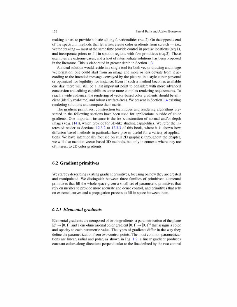
While the extent of an elemental gradient can be infinite, these primitives are

often used to fill-in closed shapes. Figure 1.3(a) shows a complex image created en-

tirely with linear and radial gradients. Figure 1.3(b) highlights how a linear gradient

fills a region to produce a convincing reflection. Although this example is com-

pelling, it requires advanced skills and a lot of time to complete a drawing. This is

why elemental gradients are most of the time confined to simple compositions.

6.2.2 Gradient meshes

The main idea of a gradient mesh is to decompose the image plane into a connected

set of simple 2D patches Pi : R2→ [0,1]2, and assign each patch a color based

on a two-dimensional color gradient [0,1]2 → [0,1]4. It improves on the elemental

-6

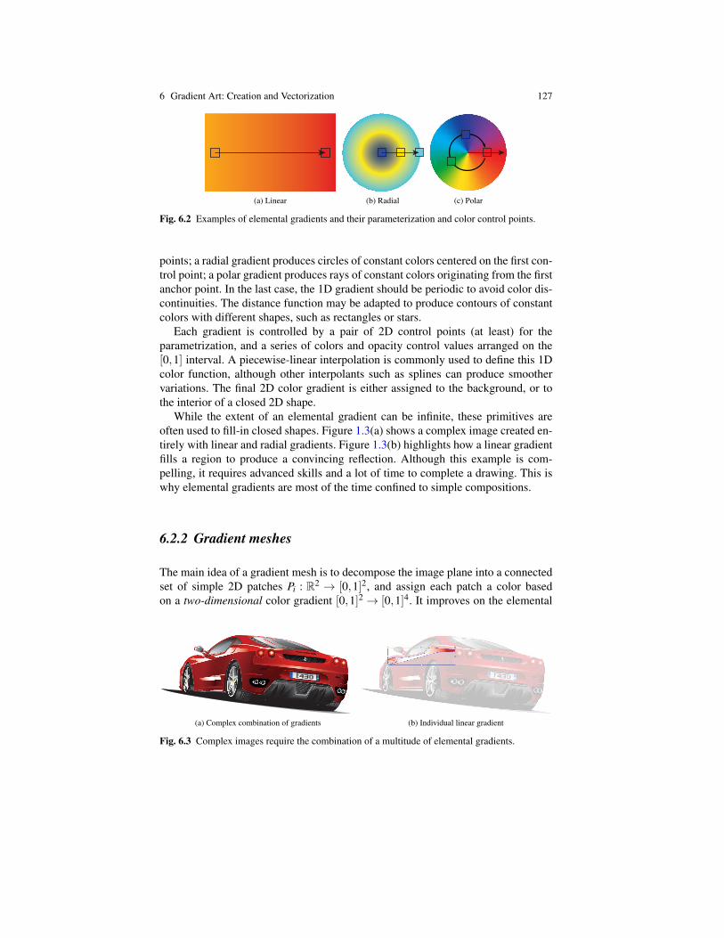
(a) Complex combination of gradients (b) Individual linear gradient

Fig. 6.3 Complex images require the combination of a multitude of elemental gradients.


(a) Control points and tangents (b) Interpolated colors

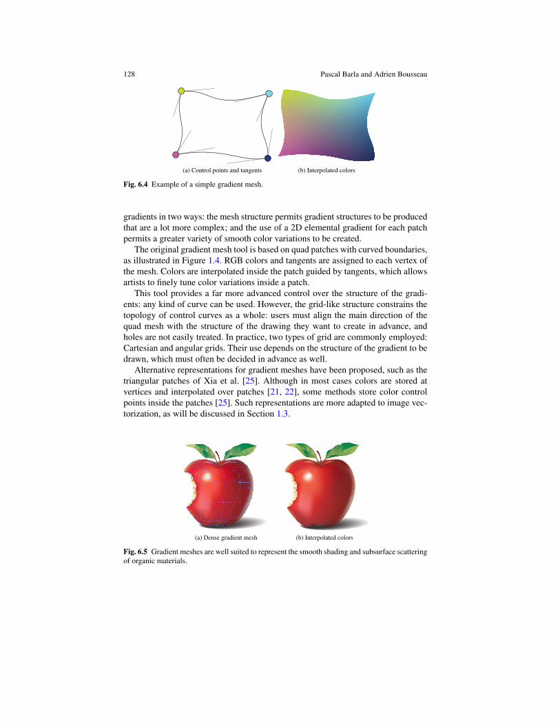
Fig. 6.4 Example of a simple gradient mesh.

gradients in two ways: the mesh structure permits gradient structures to be produced

that are a lot more complex; and the use of a 2D elemental gradient for each patch

permits a greater variety of smooth color variations to be created.

The original gradient mesh tool is based on quad patches with curved boundaries,

as illustrated in Figure 1.4. RGB colors and tangents are assigned to each vertex of

the mesh. Colors are interpolated inside the patch guided by tangents, which allows

artists to finely tune color variations inside a patch.

This tool provides a far more advanced control over the structure of the gradi-

ents: any kind of curve can be used. However, the grid-like structure constrains the

topology of control curves as a whole: users must align the main direction of the

quad mesh with the structure of the drawing they want to create in advance, and

holes are not easily treated. In practice, two types of grid are commonly employed:

Cartesian and angular grids. Their use depends on the structure of the gradient to be

drawn, which must often be decided in advance as well.

Alternative representations for gradient meshes have been proposed, such as the

triangular patches of Xia et al. [25]. Although in most cases colors are stored at

vertices and interpolated over patches [21, 22], some methods store color control

points inside the patches [25]. Such representations are more adapted to image vec-

torization, as will be discussed in Section 1.3.

(a) Dense gradient mesh (b) Interpolated colors

Fig. 6.5 Gradient meshes are well suited to represent the smooth shading and subsurface scattering

of organic materials.


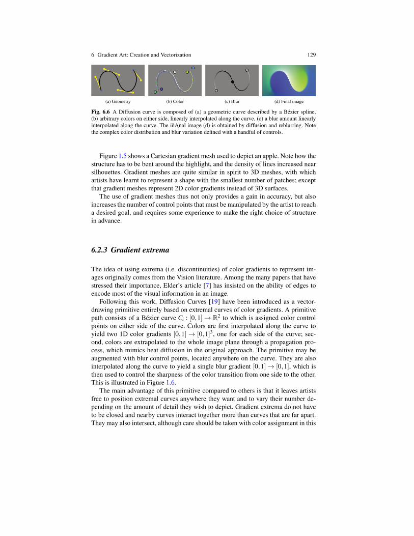
(a) Geometry (b) Color (c) Blur (d) Final image

Fig. 6.6 A Diffusion curve is composed of (a) a geometric curve described by a Bézier spline,

(b) arbitrary colors on either side, linearly interpolated along the curve, (c) a blur amount linearly

interpolated along the curve. The ïnAnal image (d) is obtained by diffusion and reblurring. Note

the complex color distribution and blur variation defined with a handful of controls.

Figure 1.5 shows a Cartesian gradient mesh used to depict an apple. Note how the

structure has to be bent around the highlight, and the density of lines increased near

silhouettes. Gradient meshes are quite similar in spirit to 3D meshes, with which

artists have learnt to represent a shape with the smallest number of patches; except

that gradient meshes represent 2D color gradients instead of 3D surfaces.

The use of gradient meshes thus not only provides a gain in accuracy, but also

increases the number of control points that must be manipulated by the artist to reach

a desired goal, and requires some experience to make the right choice of structure

in advance.

6.2.3 Gradient extrema

The idea of using extrema (i.e. discontinuities) of color gradients to represent im-

ages originally comes from the Vision literature. Among the many papers that have

stressed their importance, Elder’s article [7] has insisted on the ability of edges to

encode most of the visual information in an image.

Following this work, Diffusion Curves [19] have been introduced as a vector-

drawing primitive entirely based on extremal curves of color gradients. A primitive

path consists of a Bézier curve Ci : [0,1] → R2 to which is assigned color control

points on either side of the curve. Colors are first interpolated along the curve to

yield two 1D color gradients [0,1] → [0,1]3, one for each side of the curve; sec-

ond, colors are extrapolated to the whole image plane through a propagation pro-

cess, which mimics heat diffusion in the original approach. The primitive may be

augmented with blur control points, located anywhere on the curve. They are also

interpolated along the curve to yield a single blur gradient [0,1] → [0,1], which is

then used to control the sharpness of the color transition from one side to the other.

This is illustrated in Figure 1.6.

The main advantage of this primitive compared to others is that it leaves artists

free to position extremal curves anywhere they want and to vary their number de-

pending on the amount of detail they wish to depict. Gradient extrema do not have

to be closed and nearby curves interact together more than curves that are far apart.

They may also intersect, although care should be taken with color assignment in this


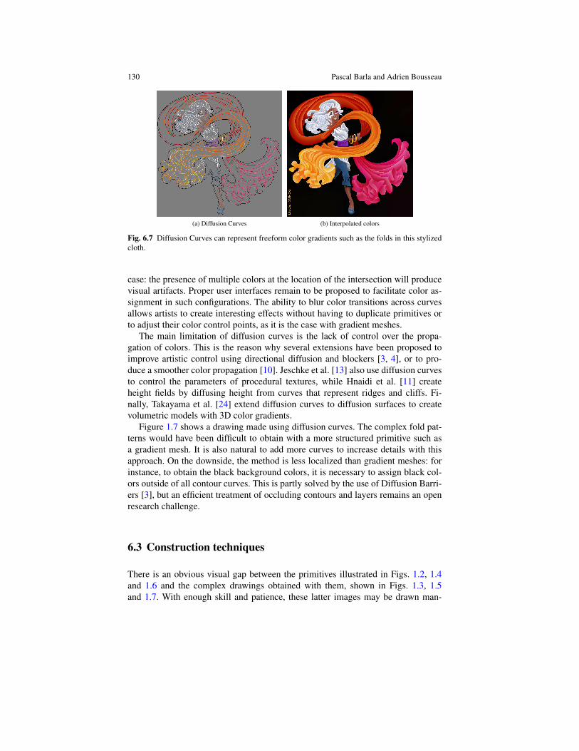
(a) Diffusion Curves (b) Interpolated colors

Fig. 6.7 Diffusion Curves can represent freeform color gradients such as the folds in this stylized

cloth.

case: the presence of multiple colors at the location of the intersection will produce

visual artifacts. Proper user interfaces remain to be proposed to facilitate color as-

signment in such configurations. The ability to blur color transitions across curves

allows artists to create interesting effects without having to duplicate primitives or

to adjust their color control points, as it is the case with gradient meshes.

The main limitation of diffusion curves is the lack of control over the propa-

gation of colors. This is the reason why several extensions have been proposed to

improve artistic control using directional diffusion and blockers [3, 4], or to pro-

duce a smoother color propagation [10]. Jeschke et al. [13] also use diffusion curves

to control the parameters of procedural textures, while Hnaidi et al. [11] create

height fields by diffusing height from curves that represent ridges and cliffs. Fi-

nally, Takayama et al. [24] extend diffusion curves to diffusion surfaces to create

volumetric models with 3D color gradients.

Figure 1.7 shows a drawing made using diffusion curves. The complex fold pat-

terns would have been difficult to obtain with a more structured primitive such as

a gradient mesh. It is also natural to add more curves to increase details with this

approach. On the downside, the method is less localized than gradient meshes: for

instance, to obtain the black background colors, it is necessary to assign black col-

ors outside of all contour curves. This is partly solved by the use of Diffusion Barri-

ers [3], but an efficient treatment of occluding contours and layers remains an open

research challenge.

6.3 Construction techniques

There is an obvious visual gap between the primitives illustrated in Figs. 1.2, 1.4

and 1.6 and the complex drawings obtained with them, shown in Figs. 1.3, 1.5

and 1.7. With enough skill and patience, these latter images may be drawn man-


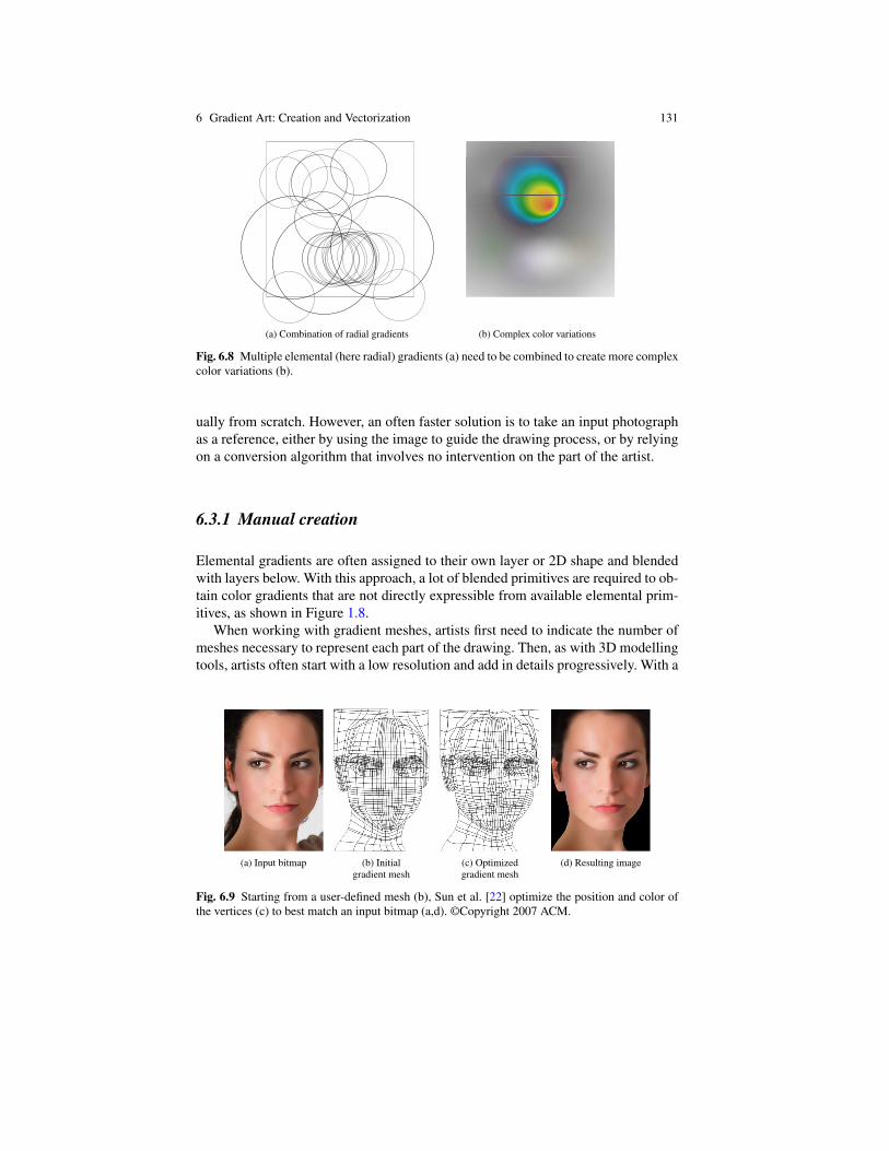
(a) Combination of radial gradients (b) Complex color variations

Fig. 6.8 Multiple elemental (here radial) gradients (a) need to be combined to create more complex

color variations (b).

ually from scratch. However, an often faster solution is to take an input photograph

as a reference, either by using the image to guide the drawing process, or by relying

on a conversion algorithm that involves no intervention on the part of the artist.

6.3.1 Manual creation

Elemental gradients are often assigned to their own layer or 2D shape and blended

with layers below. With this approach, a lot of blended primitives are required to ob-

tain color gradients that are not directly expressible from available elemental prim-

itives, as shown in Figure 1.8.

When working with gradient meshes, artists first need to indicate the number of

meshes necessary to represent each part of the drawing. Then, as with 3D modelling

tools, artists often start with a low resolution and add in details progressively. With a

(a) Input bitmap (b) Initial

gradient mesh

(c) Optimized

gradient mesh

(d) Resulting image

Fig. 6.9 Starting from a user-defined mesh (b), Sun et al. [22] optimize the position and color of

the vertices (c) to best match an input bitmap (a,d). ©Copyright 2007 ACM.


regular quad-based mesh, users can add vertical or horizontal curves, move control

points and assign them new colors. Finer meshes are often needed to draw objects

with complex topology.

When a reference image is available, the mesh can be aligned with the image

features by hand, and vertex colors can be automatically sampled from underlying

pixels. A faster solution is to use optimisation techniques [21, 22] that optimize

the color and position of vertices to best match the input image, as illustrated in

Figure 1.9. Even if these methods are not entirely automatic, they save a lot of time

for artists.

Alternative structures that work with triangular meshes for instance are a lot

harder to draw entirely from scratch: the overall structure has to be changed when

one wants to add details or move some parts of the structure. This is why such meth-

ods have been rather confined to automatic conversion.

When working with gradient extrema such as diffusion curves, a simple strategy

consists of first drawing the curves as a line drawing, and then adding or editing

colors and blur transitions along each curve. This approach is somewhat similar

to the traditional “sketching + coloring” process in traditional drawing. Because

of their flexibility, extremal primitives are also well adapted to multi-touch user

interfaces [23]. To facilitate color editing, Jeschke et al. [13] propose storing for

each pixel a list of the most influential curves and color control points. Users can

then specify the color at a pixel to modify the color of the curves accordingly.

When a reference image is available, active contours [15] can be used to snap

extremal curves to image locations where the color gradient is strong [19]. To as-

sign color values, two methods have been proposed. A direct solution consists in

sampling a dense set of color control points along each side of a curve directly

from the image, and then simplifying the set of samples by keeping only the most

relevant ones using the Douglas-Pucker algorithm [19]. However, this method still

requires many color control points to reach satisfying results. A better solution, pro-

posed by Jeschke et al. [13], consists in finding optimal color control points using a

least-squares approach.

6.3.2 Automatic conversion

The earliest of automatic conversion methods were designed for image compres-

sion purposes, and relied on simple triangulations [6]. One of the first techniques

that presented vectorization for stylization purposes is the Ardeco system [17] that

converts bitmap images into linear or radial gradients. The core of this method is a

region segmentation algorithm based on an energy minimization that combines two

terms: one term aims at creating compact regions while the other term measures the

goodness of fit of elemental color gradients.

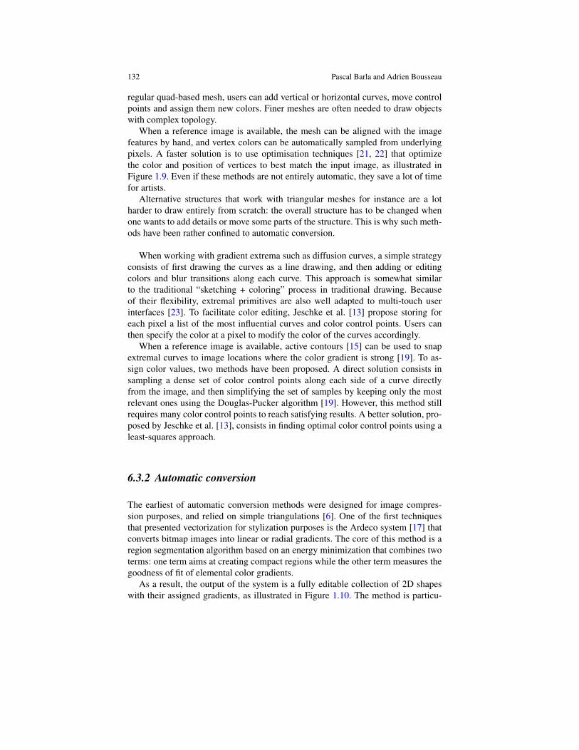
As a result, the output of the system is a fully editable collection of 2D shapes

with their assigned gradients, as illustrated in Figure 1.10. The method is particu-


(a) Input bitmap (b) Segmentation (c) Linear gradient approximation

Fig. 6.10 The Ardeco system [17] converts an input bitmap into a collection of linear or radial

gradients. The algorithms segments the image into regions well approximated by the elemental

gradients. ©Copyright 2006 Eurographics.

larly efficient at converting images of artwork composed of very smooth gradients

and very sharp transitions, hence the name of the system which is reminiscent of the

artistic movement of the twenties.

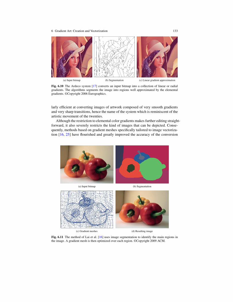
Although the restriction to elemental color gradients makes further editing straight-

forward, it also severely restricts the kind of images that can be depicted. Conse-

quently, methods based on gradient meshes specifically tailored to image vectoriza-

tion [16, 25] have flourished and greatly improved the accuracy of the conversion

(a) Input bitmap (b) Segmentation

(c) Gradient meshes (d) Resulting image

Fig. 6.11 The method of Lai et al. [16] uses image segmentation to identify the main regions in

the image. A gradient mesh is then optimized over each region. ©Copyright 2009 ACM.


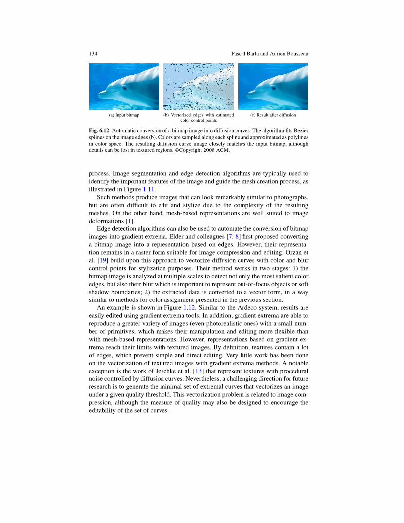
(a) Input bitmap (b) Vectorized edges with estimated

color control points

(c) Result after diffusion

Fig. 6.12 Automatic conversion of a bitmap image into diffusion curves. The algorithm fits Bezier

splines on the image edges (b). Colors are sampled along each spline and approximated as polylines

in color space. The resulting diffusion curve image closely matches the input bitmap, although

details can be lost in textured regions. ©Copyright 2008 ACM.

process. Image segmentation and edge detection algorithms are typically used to

identify the important features of the image and guide the mesh creation process, as

illustrated in Figure 1.11.

Such methods produce images that can look remarkably similar to photographs,

but are often difficult to edit and stylize due to the complexity of the resulting

meshes. On the other hand, mesh-based representations are well suited to image

deformations [1].

Edge detection algorithms can also be used to automate the conversion of bitmap

images into gradient extrema. Elder and colleagues [7, 8] first proposed converting

a bitmap image into a representation based on edges. However, their representa-

tion remains in a raster form suitable for image compression and editing. Orzan et

al. [19] build upon this approach to vectorize diffusion curves with color and blur

control points for stylization purposes. Their method works in two stages: 1) the

bitmap image is analyzed at multiple scales to detect not only the most salient color

edges, but also their blur which is important to represent out-of-focus objects or soft

shadow boundaries; 2) the extracted data is converted to a vector form, in a way

similar to methods for color assignment presented in the previous section.

An example is shown in Figure 1.12. Similar to the Ardeco system, results are

easily edited using gradient extrema tools. In addition, gradient extrema are able to

reproduce a greater variety of images (even photorealistic ones) with a small num-

ber of primitives, which makes their manipulation and editing more flexible than

with mesh-based representations. However, representations based on gradient ex-

trema reach their limits with textured images. By definition, textures contain a lot

of edges, which prevent simple and direct editing. Very little work has been done

on the vectorization of textured images with gradient extrema methods. A notable

exception is the work of Jeschke et al. [13] that represent textures with procedural

noise controlled by diffusion curves. Nevertheless, a challenging direction for future

research is to generate the minimal set of extremal curves that vectorizes an image

under a given quality threshold. This vectorization problem is related to image com-

pression, although the measure of quality may also be designed to encourage the

editability of the set of curves.


I(u,v)P

00

P10P

11

P01

C1(u) C

3(u)

C2(v)

C4(v)

I1(u,v) = vC

1(u) + (1-v)C

3(u)

I2(u,v) = uC

2(v) + (1-u)C

4(v)

P(u,v) = (1-u)(1-v)P00

+ (1-u)vP01

+ u(1-v)P10

+ uvP11

I(u,v) = I1(u,v) + I

2(u,v) - P(u,v)

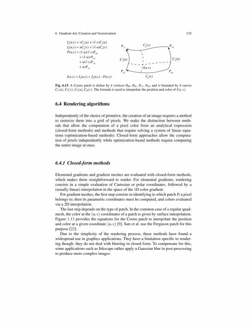
Fig. 6.13 A Coons patch is define by 4 vertices P00, P01, P11, P10, and is bounded by 4 curves

C1(u), C2(v), C3(u), C4(v). The formula is used to interpolate the position and color of I(u,v).

6.4 Rendering algorithms

Independently of the choice of primitive, the creation of an image requires a method

to rasterize them into a grid of pixels. We make the distinction between meth-

ods that allow the computation of a pixel color from an analytical expression

(closed-form methods) and methods that require solving a system of linear equa-

tions (optimization-based methods). Closed-form approaches allow the computa-

tion of pixels independently while optimization-based methods require computing

the entire image at once.

6.4.1 Closed-form methods

Elemental gradients and gradient meshes are evaluated with closed-form methods,

which makes them straightforward to render. For elemental gradients, rendering

consists in a simple evaluation of Cartesian or polar coordinates, followed by a

(usually linear) interpolation in the space of the 1D color gradient.

For gradient meshes, the first step consists in identifying to which patch Pi a pixel

belongs to; then its parametric coordinates must be computed, and colors evaluated

via a 2D interpolation.

The last step depends on the type of patch. In the common case of a regular quad-

mesh, the color at the (u,v) coordinates of a patch is given by surface interpolation.

Figure 1.13 provides the equations for the Coons patch to interpolate the position

and color at a given coordinate (u,v) [9]. Sun et al. use the Ferguson patch for this

purpose [22].

Due to the simplicity of the rendering process, these methods have found a

widespread use in graphics applications. They have a limitation specific to render-

ing though: they do not deal with blurring in closed form. To compensate for this,

some applications such as Inkscape rather apply a Gaussian blur in post-processing

to produce more complex images.


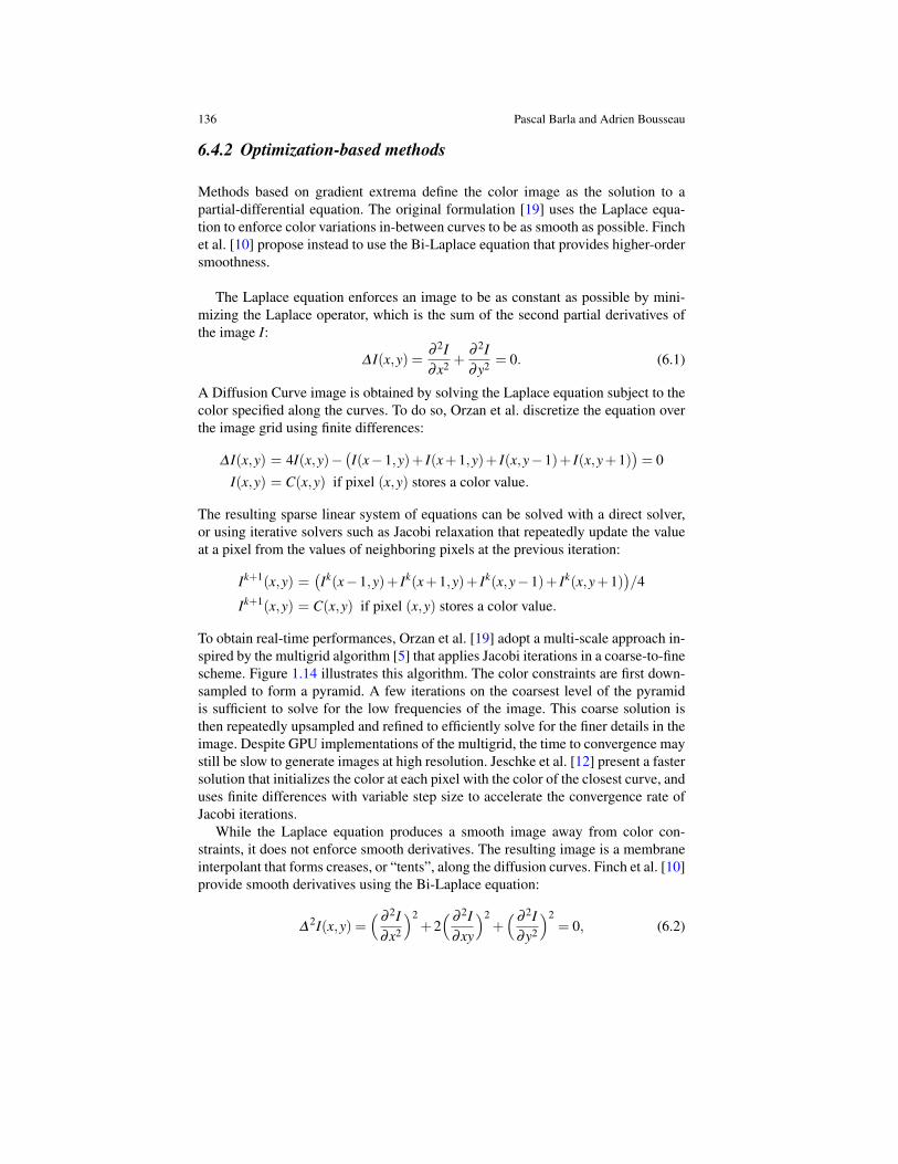
6.4.2 Optimization-based methods

Methods based on gradient extrema define the color image as the solution to a

partial-differential equation. The original formulation [19] uses the Laplace equa-

tion to enforce color variations in-between curves to be as smooth as possible. Finch

et al. [10] propose instead to use the Bi-Laplace equation that provides higher-order

smoothness.

The Laplace equation enforces an image to be as constant as possible by mini-

mizing the Laplace operator, which is the sum of the second partial derivatives of

the image I:

∆ I(x,y) =∂ 2I

∂x2+

∂ 2I

∂y2= 0. (6.1)

A Diffusion Curve image is obtained by solving the Laplace equation subject to the

color specified along the curves. To do so, Orzan et al. discretize the equation over

the image grid using finite differences:

∆ I(x,y) = 4I(x,y)−(

I(x−1,y)+ I(x+1,y)+ I(x,y−1)+ I(x,y+1))

= 0

I(x,y) = C(x,y) if pixel (x,y) stores a color value.

The resulting sparse linear system of equations can be solved with a direct solver,

or using iterative solvers such as Jacobi relaxation that repeatedly update the value

at a pixel from the values of neighboring pixels at the previous iteration:

Ik+1(x,y) =(

Ik(x−1,y)+ Ik(x+1,y)+ Ik(x,y−1)+ Ik(x,y+1))

/4

Ik+1(x,y) = C(x,y) if pixel (x,y) stores a color value.

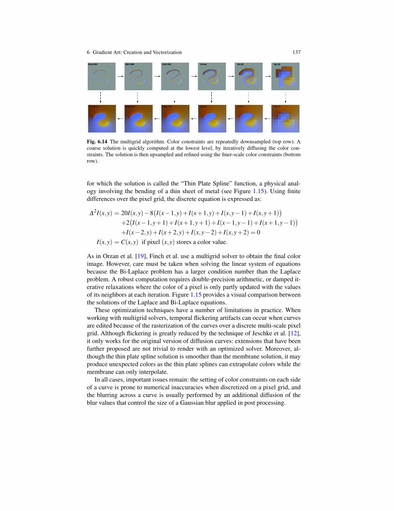
To obtain real-time performances, Orzan et al. [19] adopt a multi-scale approach in-

spired by the multigrid algorithm [5] that applies Jacobi iterations in a coarse-to-fine

scheme. Figure 1.14 illustrates this algorithm. The color constraints are first down-

sampled to form a pyramid. A few iterations on the coarsest level of the pyramid

is sufficient to solve for the low frequencies of the image. This coarse solution is

then repeatedly upsampled and refined to efficiently solve for the finer details in the

image. Despite GPU implementations of the multigrid, the time to convergence may

still be slow to generate images at high resolution. Jeschke et al. [12] present a faster

solution that initializes the color at each pixel with the color of the closest curve, and

uses finite differences with variable step size to accelerate the convergence rate of

Jacobi iterations.

While the Laplace equation produces a smooth image away from color con-

straints, it does not enforce smooth derivatives. The resulting image is a membrane

interpolant that forms creases, or “tents”, along the diffusion curves. Finch et al. [10]

provide smooth derivatives using the Bi-Laplace equation:

∆2I(x,y) =

(

∂ 2I

∂x2

)2

+2(

∂ 2I

∂xy

)2

+(

∂ 2I

∂y2

)2

= 0, (6.2)


Fig. 6.14 The multigrid algorithm. Color constraints are repeatedly downsampled (top row). A

coarse solution is quickly computed at the lowest level, by iteratively diffusing the color con-

straints. The solution is then upsampled and refined using the finer-scale color constraints (bottom

row).

for which the solution is called the “Thin Plate Spline” function, a physical anal-

ogy involving the bending of a thin sheet of metal (see Figure 1.15). Using finite

differences over the pixel grid, the discrete equation is expressed as:

∆2I(x,y) = 20I(x,y)−8

(

I(x−1,y)+ I(x+1,y)+ I(x,y−1)+ I(x,y+1))

+2(

I(x−1,y+1)+ I(x+1,y+1)+ I(x−1,y−1)+ I(x+1,y−1))

+I(x−2,y)+ I(x+2,y)+ I(x,y−2)+ I(x,y+2) = 0

I(x,y) = C(x,y) if pixel (x,y) stores a color value.

As in Orzan et al. [19], Finch et al. use a multigrid solver to obtain the final color

image. However, care must be taken when solving the linear system of equations

because the Bi-Laplace problem has a larger condition number than the Laplace

problem. A robust computation requires double-precision arithmetic, or damped it-

erative relaxations where the color of a pixel is only partly updated with the values

of its neighbors at each iteration. Figure 1.15 provides a visual comparison between

the solutions of the Laplace and Bi-Laplace equations.

These optimization techniques have a number of limitations in practice. When

working with multigrid solvers, temporal flickering artifacts can occur when curves

are edited because of the rasterization of the curves over a discrete multi-scale pixel

grid. Although flickering is greatly reduced by the technique of Jeschke et al. [12],

it only works for the original version of diffusion curves: extensions that have been

further proposed are not trivial to render with an optimized solver. Moreover, al-

though the thin plate spline solution is smoother than the membrane solution, it may

produce unexpected colors as the thin plate splines can extrapolate colors while the

membrane can only interpolate.

In all cases, important issues remain: the setting of color constraints on each side

of a curve is prone to numerical inaccuracies when discretized on a pixel grid, and

the blurring across a curve is usually performed by an additional diffusion of the

blur values that control the size of a Gaussian blur applied in post processing.


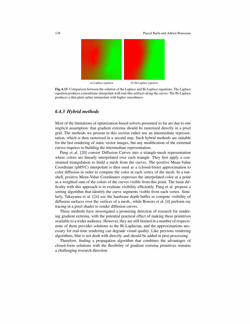
(a) Laplace equation (b) Bi-Laplace equation

Fig. 6.15 Comparison between the solution of the Laplace and Bi-Laplace equations. The Laplace

equation produces a membrane interpolant with tent-like artifacts along the curves. The Bi-Laplace

produces a thin-plate spline interpolant with higher smoothness.

6.4.3 Hybrid methods

Most of the limitations of optimisation-based solvers presented so far are due to one

implicit assumption: that gradient extrema should be rasterized directly in a pixel

grid. The methods we present in this section rather use an intermediate represen-

tation, which is then rasterized in a second step. Such hybrid methods are suitable

for the fast rendering of static vector images, but any modification of the extremal

curves requires re-building the intermediate representation.

Pang et al. [20] convert Diffusion Curves into a triangle-mesh representation

where colors are linearly interpolated over each triangle. They first apply a con-

strained triangulation to build a mesh from the curves. The positive Mean-Value

Coordinate (pMVC) interpolant is then used as a (closed-form) approximation to

color diffusion in order to compute the color at each vertex of the mesh. In a nut-

shell, positive Mean-Value Coordinates expresses the interpolated color at a point

as a weighted sum of the colors of the curves visible from this point. The main dif-

ficulty with this approach is to evaluate visibility efficiently. Pang et al. propose a

sorting algorithm that identify the curve segments visible from each vertex. Simi-

larly, Takayama et al. [24] use the hardware depth buffer to compute visibility of

diffusion surfaces over the vertices of a mesh., while Bowers et al. [4] perform ray

tracing in a pixel shader to render diffusion curves.

These methods have investigated a promising direction of research for render-

ing gradient extrema, with the potential practical effect of making these primitives

available to a wider audience. However, they are still limited in a number of respects:

none of them provides solutions to the Bi-Laplacian, and the approximations nec-

essary for real-time rendering can degrade visual quality. Like previous rendering

algorithms, blur is not dealt with directly, and should be added in post-processing.

Therefore, finding a propagation algorithm that combines the advantages of

closed-form solutions with the flexibility of gradient extrema primitives remains

a challenging research direction.


6.5 Discussion

We have presented vector primitives dedicated to the creation of color gradients,

along with methods to construct them and algorithms to render images out of them.

As of now, elemental gradients are ubiquitous in vector applications, and since gra-

dient meshes have appeared in Adobe Illustrator, they have acquired support from a

large base of users. However, only basic construction methods are available in vec-

tor graphics packages, and non-regular meshes are still confined to the vectorization

of photographs. Diffusion Curves have appeared in various forms (standalone appli-

cations, webGL), but the issues raised by rendering algorithms makes it hard to run

them on all platforms, since they often require advanced GPUs.

Gradient extrema are thus mainly limited regarding rendering, although in some

instances it is easier to use gradient meshes because the control over interiors is

more direct. On the other hand, gradient meshes are straightforward to render, but

often tend to produce too dense representations. This tradeoff is reflected by the

open scientific challenges we gave hints at throughout the chapter.

There might be a greater challenge though. To understand it, imagine placing the

methods we have presented on an axis ranging from those more prone to creation, to

those more adapted to conversion. Methods based on gradient extrema will cluster

on the creation side, while those based on gradient meshes will rather be packed on

the conversion side. In other words, there is a “virgin land” that has not yet been

reached, and it might necessitate the invention of yet another kind of primitive, that

better accounts for the structure found in images while still being sparse enough to

promote direct, intuitive control.

Throughout this chapter we have only considered static images, but another ap-

peal of vector graphics is animation. For instance, rotoscoping methods might make

use of patches and curves to track image features from frame to frame and vector-

ize them. Then least-square optimizations could be employed to assign them colors

smoothly in both space and time. Finally, these color gradients could serve as base

layers to guide further stylization processes, hence finding their place in stylized

rendering pipelines.

References

1. Barrett, W.A., Cheney, A.S.: Object-based image editing. ACM TOG (Proc. SIGGRAPH)

21(3), 777–784 (2002). DOI 10.1145/566654.566651

2. Baxter, W.V., Scheib, V., Lin, M.C.: dAb: Interactive Haptic Painting With 3D Virtual Brushes.

In: SIGGRAPH, pp. 461–468 (2001)

3. Bezerra, H., Eisemann, E., DeCarlo, D., Thollot, J.: Diffusion constraints for vector graph-

ics. In: Proceedings of the International Symposium on Non-Photorealistic Animation and

Rendering (NPAR), pp. 35–42 (2010). DOI 10.1145/1809939.1809944

4. Bowers, J.C., Leahey, J., Wang, R.: A Ray Tracing Approach to Diffusion Curves. Computer

Graphics Forum (Proc. EGSR) 30(4), 1345–1352 (2011). DOI 10.1111/j.1467-8659.2011.

01994.x


5. Briggs, W.L., Henson, V.E., McCormick, S.F.: A multigrid tutorial. Society for Industrial and

Applied Mathematics (2000)

6. Demaret, L., Dyn, N., Iske, A.: Image compression by linear splines over adaptive triangula-

tions. Signal Process. 86(7), 1604–1616 (2006). DOI 10.1016/j.sigpro.2005.09.003

7. Elder, J.H.: Are Edges Incomplete? Int. J. Comput. Vision 34(2–3), 97–122 (1999). DOI

10.1023/A:1008183703117

8. Elder, J.H., Goldberg, R.M.: Image Editing in the Contour Domain. IEEE Trans. Pattern Anal.

Mach. Intell. 23(3), 291–296 (2001). DOI 10.1109/34.910881

9. Farin, G., Hansford, D.: Discrete Coons patches. Computer Aided Geometric Design 16,

691–700 (1999)

10. Finch, M., Snyder, J., Hoppe, H.: Freeform vector graphics with controlled thin-plate splines.

ACM Transactions on Graphics (Proc. SIGGRAPH Asia) 30(6), 166:1–166:10 (2011). DOI

10.1145/2070781.2024200

11. Hnaidi, H., Guérin, E., Akkouche, S., Peytavie, A., Galin, E.: Feature based terrain generation

using diffusion equation. Computer Graphics Forum (Proceedings of Pacific Graphics) 29(7),

2179–2186 (2010)

12. Jeschke, S., Cline, D., Wonka, P.: A GPU Laplacian solver for diffusion curves and Poisson

image editing. ACM Transactions on Graphics (Proc. SIGGRAPH Asia) 28, 116:1–116:8

(2009). DOI 10.1145/1618452.1618462

13. Jeschke, S., Cline, D., Wonka, P.: Estimating Color and Texture Parameters for Vector Graph-

ics. Computer Graphics Forum (Proc. Eurographics) 30(2), 523–532 (2011)

14. Johnston, S.F.: Lumo: illumination for cel animation. In: Proceedings of the international

symposium on Non-photorealistic animation and rendering (NPAR) (2002). DOI 10.1145/

508530.508538

15. Kass, M., Witkin, A., Terzopoulos, D.: Snakes: Active contour models. International Journal

of Computer Vision 1(4), 321–331 (1988)

16. Lai, Y.K., Hu, S.M., Martin, R.R.: Automatic and topology-preserving gradient mesh gen-

eration for image vectorization. ACM Trans. Graph. 28(3), 85:1–85:8 (2009). DOI

10.1145/1531326.1531391

17. Lecot, G., Lévy, B.: ARDECO: Automatic Region DEtection and Conversion. In: 17th Euro-

graphics Symposium on Rendering - EGSR’06, pp. 349–360 (2006)

18. McCann, J., Pollard, N.S.: Real-Time Gradient-Domain Painting. ACM TOG (Proc. SIG-

GRAPH) 27(3), 93:1–93:7 (2008)

19. Orzan, A., Bousseau, A., Winnemöller, H., Barla, P., Thollot, J., Salesin, D.: Diffusion curves:

a vector representation for smooth-shaded images. ACM Transactions on Graphics (Proc.

SIGGRAPH) 27, 92:1–92:8 (2008). DOI http://doi.acm.org/10.1145/1360612.1360691

20. Pang, W.M., Qin, J., Cohen, M., Heng, P.A., Choi, K.S.: Fast Rendering of Diffusion Curves

with Triangles. IEEE Computer Graphics and Applications 99(PrePrints) (2011). DOI 10.

1109/MCG.2011.86

21. Price, B.L., Barrett, W.A.: Object-based vectorization for interactive image editing. The Visual

Computer 22(9-11), 661–670 (2006). DOI 10.1007/s00371-006-0051-1

22. Sun, J., Liang, L., Wen, F., Shum, H.Y.: Image vectorization using optimized gradient meshes.

ACM Trans. Graph. 26(3) (2007). DOI 10.1145/1276377.1276391

23. Sun, Q., Fu, C.W., He, Y.: An interactive multi-touch sketching interface for diffusion curves.

In: Proceedings of the 2011 annual conference on Human factors in computing systems (CHI),

pp. 1611–1614 (2011). DOI 10.1145/1978942.1979176

24. Takayama, K., Sorkine, O., Nealen, A., Igarashi, T.: Volumetric modeling with diffusion sur-

faces. ACM Transactions on Graphics (Proc. SIGGRAPH Asia) 29, 180:1–180:8 (2010).

DOI 10.1145/1882261.1866202

25. Xia, T., Liao, B., Yu, Y.: Patch-based image vectorization with automatic curvilinear feature

alignment. ACM Trans. Graph. 28(5), 115:1–115:10 (2009). DOI 10.1145/1618452.1618461

Documents

Gradient Art: Creation and Vectorization - Inria 6 Gradient Art: Creation and Vectorization Pascal Barla and Adrien Bousseau Abstract There are two different categories of methods