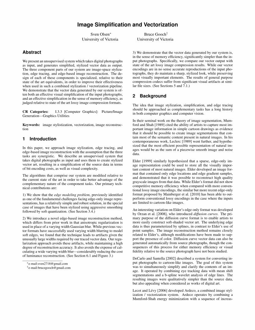
Image Simplification and Vectorization

Sven Olsen∗

University of VictoriaBruce Gooch†

University of Victoria

Abstract

We present an unsupervised system which takes digital photographsas input, and generates simplified, stylized vector data as output.The three component parts of our system are image-space styliza-tion, edge tracing, and edge-based image reconstruction. The de-sign of each of these components is specialized, relative to theirstate of the art equivalents, in order to improve their effectivenesswhen used in such a combined stylization / vectorization pipeline.We demonstrate that the vector data generated by our system is of-ten both an effective visual simplification of the input photographs,and an effective simplification in the sense of memory efficiency, asjudged relative to state of the art lossy image compression formats.

CR Categories: I.3.3 [Computer Graphics]: Picture/ImageGeneration—Graphics Utilities

Keywords: image stylistization, vectorization, image reconstruc-tion

1 Introduction

In this paper, we approach image stylization, edge tracing, andedge-based image reconstruction with the assumption that the threetasks are synergistic. We describe an unsupervised system thattakes digital photographs as input and uses them to create stylizedvector art, resulting in a simplification of the source data in termsof bit encoding costs, as well as visual complexity.

The algorithms that comprise our system are modified relative tothe current state of the art in order to take better advantage of thecomplementary nature of the component tasks. Our primary tech-nical contributions are:

1) We show that the edge modeling problem, previously identifiedas one of the fundamental challenges facing edge-only image repre-sentations, has a relatively simple and robust solution, in the specialcase of images that have been stylized using aggressive smoothingfollowed by soft quantization. (See Section 3.4.)

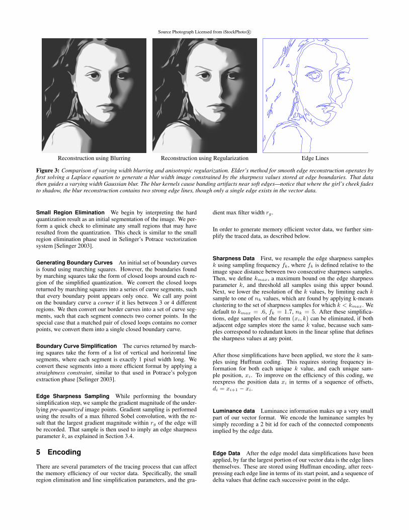
2) We introduce a novel edge-based image reconstruction method,which differs from prior work in that anisotropic regularization isused in place of a varying width Gaussian blur. While previous vec-tor formats have successfully used varying width blurring to modelsoft edges, we found that the technique leads to artifacts given theunusually large widths required by our traced vector data. Our regu-larization approach avoids these artifacts, while maintaining a highdegree of reconstruction accuracy. It also avoids the expense of cal-culating a wide varying width blur—considerably reducing the costof luminance reconstruction. (See Section 6.1 and Figure 3.)

∗e-mail:sven2718@gmail.com†e-mail:brucegooch@gmail.com

3) We demonstrate that the vector data generated by our system is,in the sense of memory efficiency, significantly simpler than the in-put photographs. Specifically, we compare our vector output withstate of the art lossy image compression results. While our vectorencodings are in no sense accurate reproductions of the input pho-tographs, they do maintain a sharp, stylized look, while preservingmost visually important elements. The results of general purposecompression codecs suffer from significant visual artifacts at simi-lar file sizes. (See Sections 5 and 7.1.)

2 Background

The idea that image stylization, simplification, and edge tracingshould be approached as complementary tasks has a long historyin both computer graphics and computer vision.

In their seminal work on the theory of image segmentation, Mum-ford and Shah [1989] cited the ability of artists to capture most im-portant image information in simple cartoon drawings as evidencethat it should be possible to create image segmentations that con-tain most of the semantic content present in natural images. In hiscontemporaneous work, Leclerc [1989] went further, and hypothe-sized that the most efficient possible representation of natural im-ages would be as the sum of a piecewise smooth image and noisedata.

Elder [1999] similarly hypothesized that a sparse, edge-only im-age representation could be used to store all the visually impor-tant content of most natural images. Elder developed an image for-mat that contained only edge locations and edge gradient samples,and demonstrated that it was possible to reconstruct high qualitygrayscale images from that data. While Elder’s format did not showcompetitive memory efficiency when compared with more conven-tional lossy image encodings, the similar but more recent edge-onlyformat proposed by Mainberger et al. [2010] has been able to out-perform conventional lossy encodings in the case where the inputsare limited to cartoon-like images.

An interesting variation on Elder’s edge only format was developedby Orzan et al. [2008], who introduced diffusion curves. The pri-mary purpose of the diffusion curve format is to enable artists tomore easily construct soft-shaded vector art. The underlying edgedata is thus parameterized by splines, in contrast to Elder’s use ofpoint samples. The image reconstruction method remains closelyrelated to Elder’s, although modifications have been made to sup-port the presence of color. Diffusion curve vector data can also begenerated automatically from source photographs, though the con-sequences of this process for either memory efficiency or visualfidelity relative to the source photograph have not been studied.

DeCarlo and Santella [2002] described a system for converting in-put photographs to cartoon-like images. The goal of this systemwas to simultaneously simplify and clarify the contents of an im-age. It operated by combining eye tracking data with mean shiftsegmentations and a b-spline wavelet analysis of edge lines. Theresulting images were qualitatively simpler than the source data,but also appealing when considered as works of digital art.

Lecot and Levy [2006] developed Ardeco, a combined image styl-ization / vectorization system. Ardeco operates by combining aMumford-Shah energy minimization with a sequence of increas-

InputPhotograph

UnsharpMask Line Integral

Pre-QuantizedImage

StylizedSource Image

HardQuantization

Larger σ , per Equation (1)

2

Larger σ , per Equation (2)

2

Figure 1: Overview of image space simplification. The green boxes on the right show the degree to which the variance-based reparameter-ization given in equation (2) removes the influence of σ2. The unsharp mask result shown in blue is calculated with σ2 = 1.1σ1, while bothalternate results are shown with σ2 = 1.6σ1.

ingly simplified triangle meshes, which are converted to splineboundary curves at the end of the process. In an approach simi-lar to Elder’s edge image reconstruction, adaptive blurring is usedto model soft edges between regions. A study of the memory effi-ciency of Ardeco’s vector output showed that the system could, un-der some circumstances, outperform JPEG encoding, but the com-pression results were less competitive relative to the more modernJPEG2000 standard [Stoiber 2007].

Gradient meshes are a vector format capable of representing smoothshaded images. A gradient mesh uses a collection of spline patchesto parameterize smoothly varying colors over an image. Gradientmeshes are supported by vector editing programs such as AdobeIllustrator, but have traditionally required a large amount of userguidance to create. However, in 2007, Sun et al. showed thatthe task of finding an optimal gradient mesh representation of aninput image could be productively approached using a nonlinearleast squares solver [Sun et al. 2007]. Subsequent work by Xiaet al. demonstrated that arbitrary input images could be repre-sented by relatively simple gradient meshes at a very high levelof accuracy [Xia et al. 2009]. The primary motivation of gradi-ent mesh generation algorithms has been to simplify graphic designtasks [Price and Barrett 2006]; however, Sun et al. [2007] were ableto show that for simple images, their optimized gradient mesh re-sults led to more compact files than JPEG compression.

The image-space stylization filter which we present here benefitsfrom the many recent computer graphics papers that have advancedthe art and science of image space stylization. In particular, wemake use of the ability of difference of Gaussians filtering to effec-tively simplify and abstract facial features, something first noted byGooch et al. [2004]. Variations on difference of Gaussian filtering

that allow a wider range of artistic effects and higher quality resultshave since been developed by Winnemoller et al. [2006], Kang etal. [2007], and Kyprianidis and Dollner [2008]. The flow-guidedfilters introduced by Kang et al., in particular, have proven veryuseful in creating high quality stylizations for use as input to ourvector tracing and reconstruction algorithms.

3 Image Space Simplification and Stylization

The image space simplification is composed of three steps. First,the photograph is converted to grayscale, and a combination of blur-ring and unsharp masking is used to remove details and exaggerateedges. Next, an edge orientation field is generated, and used toguide a line integral convolution, thus simplifying object boundarylines. The operation finishes by applying a non-uniform soft quan-tization filter, setting most of pixels in the image to one of threemain tones. Figure 1 demonstrates the effects of each step.

3.1 Blurring and Unsharp Masking

Let Iσ denote the Gaussian blur of image I using a kernel of stan-dard deviation σ. Blurring the input image using σ1, then perform-ing an unsharp mask of strength p using a second blur result yieldsan image Im, which will have reduced details but stronger edges.If σ2 is defined to be the sum of the widths of the unsharp maskblur and σ1, then result of these first two steps can be expressed asfollows,

Im := Iσ1 + p(Iσ1 − Iσ2), where σ2 > σ1. (1)

The closer σ2 is to σ1, the larger p must be to create a noticeable

edge enhancement effect. This makes experimenting with differentparameter values tedious, as small changes to either σ value candramatically change the effect of different p values. In practice, itis helpful to reparametrize equation (1) in terms of the variance ofthe Difference of Gaussians image E := Iσ1 − Iσ2 .

Im := Iσ1 + p

√V ar(Iσ1)

V ar(E)E. (2)

As shown in Figure 1, under this parameterization the choice of σ2

proves to have very little impact on the resulting image Im. Thusmost features of the image Im can be controlled by adjusting tworelatively intuitive parameters—the base blur strength σ1, and theunsharp mask strength p. All images shown in this paper are gen-erated using σ2 := 1.1σ1, while p is typically set at .16, and σ1 istypically set to 0.2 percent of the input image width.

3.2 Line Integral Convolution

The second step simplifies object boundaries and eliminates mostof the noise introduced by unsharp masking. This is achieved byusing a smoothed edge orientation field to guide a line integral con-volution of Im. The edge orientation field is calculated using astructure tensor constructed from blurred Sobel gradient terms, asin Kyprianidis and Dollner [2008]. We typically use a structuretensor blurring parameter, σf , equal to 0.64 percent of the imagewidth.

The edge orientation field is then used to guide line integral convo-lution, with a Gaussian kernel of standard deviation σc, using themethod of Cabral et al. [1993]. As noted by Kang et al. [2007],Cabral’s method requires a slight modification in the case of edgeorientation fields, as at each sample point there are two displace-ments consistent with the edge orientation. This ambiguity is bestresolved by choosing the displacement that minimizes the bendingof the line integral’s center line.

Our system defaults to a line integral convolution strength σc equalto 1.6 percent of the image width, but, this can lead to over blurringin more detailed images. In such cases we frequently use a σc valueof 0.3.

3.3 Linear Transformation and Soft Quantization

The image is next modified in such a way that shadows andhighlights will be exaggerated. We achieve this effect by apply-ing a piecewise linear transformation chosen to map the values(.45, .75, .85) to (.2, .61, .95). We refer to the result of this trans-formation step as the pre-quantized image.

As a final step of the stylization, we apply a non-uniform soft-quantization function. The function we use is similar to the softquantization operator in Winnemoller et al. [2006], but it allowsarbitrary bin centers, and lacks the discontinuities present in theoriginal operation.

Given an ordered list of characteristic values, b = (b1, ..., bn), thehard quantization of a value v is given by,

q(v,b) := bi where bi is the characteristic value closest to v.

To create an analogous soft quantization function, we split the in-terval [b1, bn] into n − 1 regions, each of which will map to adifferent sigmoid curve. For v ∈ [b1, bn], let bi be the closestcharacteristic value to v. Now define the sigmoid curve index jas j := i − [bi ≥ v] + [v = b1] (here the square brackets areIverson notation [Graham et al. 1994]). Finally, define the width

of sigmoid j as wj := 12(bj+1 − bj), and its vertical shift as

cj := 12(bj+1 + bj). Using these variables, we create the following

non-uniform, continuous soft quantization function,

p(v, s) := wjsig( s

wj(v − cj))

sig(s)+ cj . (3)

Note that the the division by sig(s) ensures C0 continuity. Alsonote that that the derivative at the border between two quantizationregions is independent of the spacing between bins. Specifically,p′(cj , s) = s sig′(0)

sig(s). Thus the sharpness of the soft quantization is

controlled exclusively by the sharpness parameter s; it is indepen-dent of the spacing of the characteristic values. For sigmoid func-tions with sig′(0) = 1, equation (3) converges towards p(v, s) = vas s → 0. In other words, the maximally smooth soft quantizationfunction is simply the identity transform.

Given arbitrary v ∈ R, we clamp v to the interval [b1, bn], beforeapplying equation (3), this allows us to extend the domain of thesoft quantization function to all R.

In our stylization system, the non-uniform soft quantization func-tion is applied using b = (.2, .61, .95), and s = 2.

We also choose to apply soft quantization using the exponentialsigmoid sig(x), rather than more commonly seen sigmoidal curvessuch as tanh or erf .

sig(x) :=

1− e−x if x > 0,

ex − 1 otherwise.(4)

The choice of sigmoid function impacts the edge model used whenvectorizing and reconstructing the stylized image, and using the ex-ponential sigmoid in the soft quantization step implies that the dif-ferential equations in Section 6.1 have simple solutions.

After applying soft quantization, our image stylization is complete.We thus refer to the soft quantization result as the stylized sourceimage.

The boundaries between quantization regions will form the startinglines input to our tracing algorithms. As the image shadows andhighlights are exaggerated by the linear transformation, and thenquantized using bin values chosen to divide the image into extremesof light and dark regions, there is a sense in which our approachto combined stylization and vectorization follows the advice givenby Edwards [1979] in her famously effective instructional book,Drawing on the Right Side of the Brain. Rather than attempting totrace the outlines of individual objects, we simply focus on tracingpatterns of light and dark tones.

3.4 A Solution to the Edge Modeling Problem

When Elder [1999] initially proposed his edge-only image format,he identified edge modeling as a central challenge facing any edge-only format, and one that might limit the utility of edge only im-ages in practice. To solve the edge modeling problem, we must beable to characterize how image data should behave on either side ofan edge. For soft edges, simply sampling the gradient at the edgecrossing is not sufficient, it is necessary to have some model thatspecifies how luminance will vary as the distance from the edgeincreases. Elder’s solution to the edge modeling problem was to as-sume that all luminance variations across edges could be modeledby the error function erf(x). The edge model parameter k was thenfound by fitting this function to the source image data near the edge.

Elder’s edge fitting method sampled only four pixel values, but,even so, it lead to good results in the context of his own edge-based

Input Result

x

k

w

w

0

1

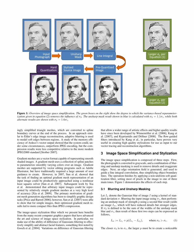
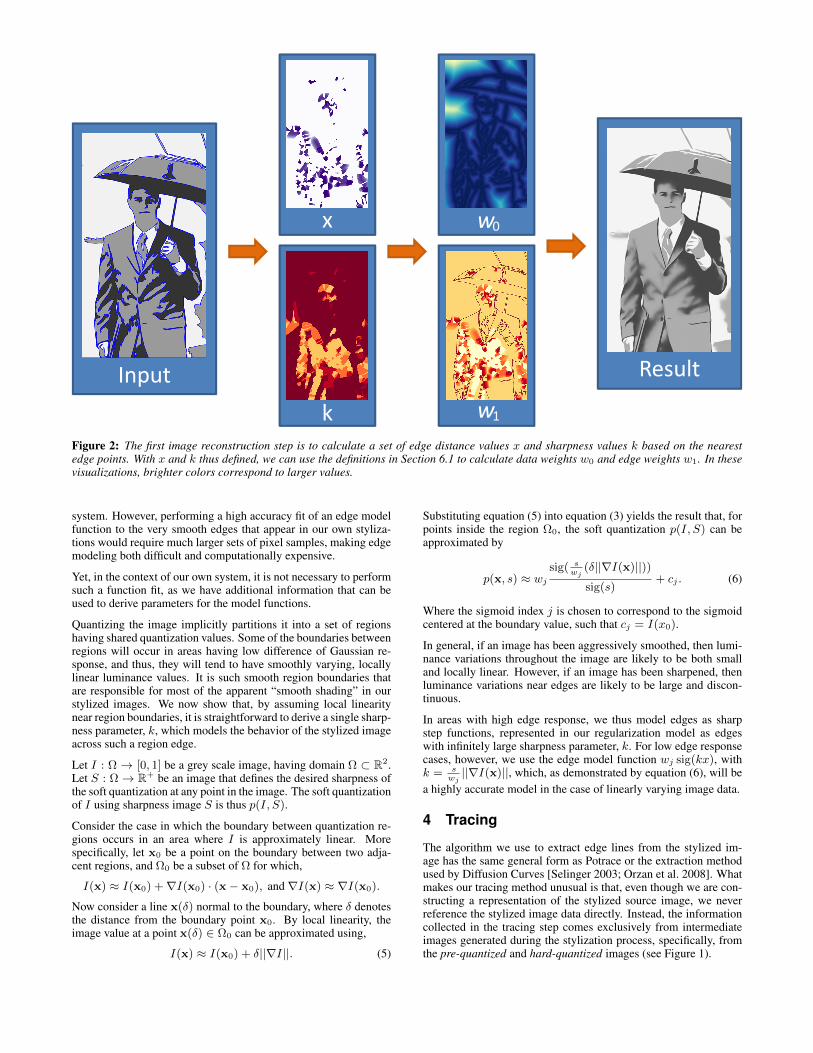
Figure 2: The first image reconstruction step is to calculate a set of edge distance values x and sharpness values k based on the nearestedge points. With x and k thus defined, we can use the definitions in Section 6.1 to calculate data weights w0 and edge weights w1. In thesevisualizations, brighter colors correspond to larger values.

system. However, performing a high accuracy fit of an edge modelfunction to the very smooth edges that appear in our own styliza-tions would require much larger sets of pixel samples, making edgemodeling both difficult and computationally expensive.

Yet, in the context of our own system, it is not necessary to performsuch a function fit, as we have additional information that can beused to derive parameters for the model functions.

Quantizing the image implicitly partitions it into a set of regionshaving shared quantization values. Some of the boundaries betweenregions will occur in areas having low difference of Gaussian re-sponse, and thus, they will tend to have smoothly varying, locallylinear luminance values. It is such smooth region boundaries thatare responsible for most of the apparent “smooth shading” in ourstylized images. We now show that, by assuming local linearitynear region boundaries, it is straightforward to derive a single sharp-ness parameter, k, which models the behavior of the stylized imageacross such a region edge.

Let I : Ω → [0, 1] be a grey scale image, having domain Ω ⊂ R2.Let S : Ω→ R+ be an image that defines the desired sharpness ofthe soft quantization at any point in the image. The soft quantizationof I using sharpness image S is thus p(I, S).

Consider the case in which the boundary between quantization re-gions occurs in an area where I is approximately linear. Morespecifically, let x0 be a point on the boundary between two adja-cent regions, and Ω0 be a subset of Ω for which,

I(x) ≈ I(x0) +∇I(x0) · (x− x0), and∇I(x) ≈ ∇I(x0).

Now consider a line x(δ) normal to the boundary, where δ denotesthe distance from the boundary point x0. By local linearity, theimage value at a point x(δ) ∈ Ω0 can be approximated using,

I(x) ≈ I(x0) + δ||∇I||. (5)

Substituting equation (5) into equation (3) yields the result that, forpoints inside the region Ω0, the soft quantization p(I, S) can beapproximated by

p(x, s) ≈ wjsig( s

wj(δ||∇I(x)||))sig(s)

+ cj . (6)

Where the sigmoid index j is chosen to correspond to the sigmoidcentered at the boundary value, such that cj = I(x0).

In general, if an image has been aggressively smoothed, then lumi-nance variations throughout the image are likely to be both smalland locally linear. However, if an image has been sharpened, thenluminance variations near edges are likely to be large and discon-tinuous.

In areas with high edge response, we thus model edges as sharpstep functions, represented in our regularization model as edgeswith infinitely large sharpness parameter, k. For low edge responsecases, however, we use the edge model function wj sig(kx), withk = s

wj||∇I(x)||, which, as demonstrated by equation (6), will be

a highly accurate model in the case of linearly varying image data.

4 Tracing

The algorithm we use to extract edge lines from the stylized im-age has the same general form as Potrace or the extraction methodused by Diffusion Curves [Selinger 2003; Orzan et al. 2008]. Whatmakes our tracing method unusual is that, even though we are con-structing a representation of the stylized source image, we neverreference the stylized image data directly. Instead, the informationcollected in the tracing step comes exclusively from intermediateimages generated during the stylization process, specifically, fromthe pre-quantized and hard-quantized images (see Figure 1).

Source Photograph Licensed from iStockPhoto R©

Reconstruction using Blurring Reconstruction using Regularization Edge Lines

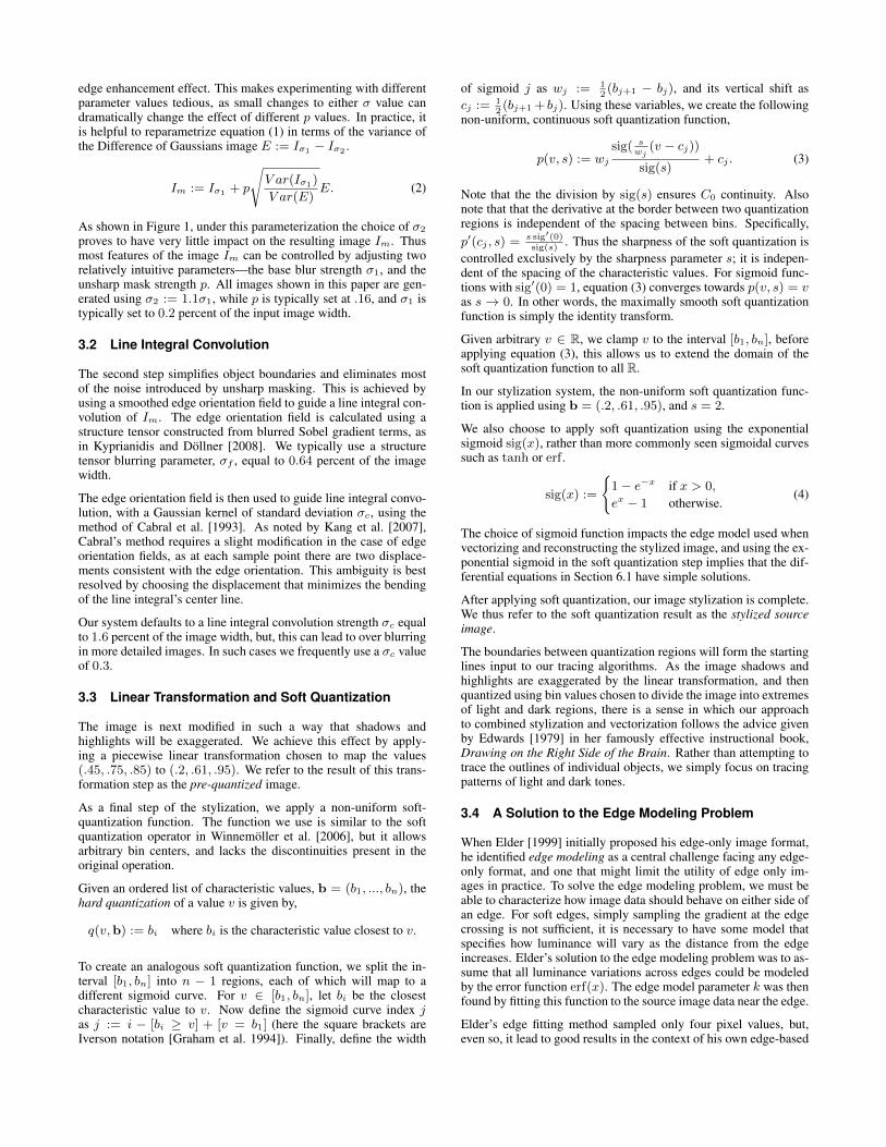
Figure 3: Comparison of varying width blurring and anisotropic regularization. Elder’s method for smooth edge reconstruction operates byfirst solving a Laplace equation to generate a blur width image constrained by the sharpness values stored at edge boundaries. That datathen guides a varying width Gaussian blur. The blur kernels cause banding artifacts near soft edges—notice that where the girl’s cheek fadesto shadow, the blur reconstruction contains two strong edge lines, though only a single edge exists in the vector data.

Small Region Elimination We begin by interpreting the hardquantization result as an initial segmentation of the image. We per-form a quick check to eliminate any small regions that may haveresulted from the quantization. This check is similar to the smallregion elimination phase used in Selinger’s Potrace vectorizationsystem [Selinger 2003].

Generating Boundary Curves An initial set of boundary curvesis found using marching squares. However, the boundaries foundby marching squares take the form of closed loops around each re-gion of the simplified quantization. We convert the closed loopsreturned by marching squares into a series of curve segments, suchthat every boundary point appears only once. We call any pointon the boundary curve a corner if it lies between 3 or 4 differentregions. We then convert our border curves into a set of curve seg-ments, such that each segment connects two corner points. In thespecial case that a matched pair of closed loops contains no cornerpoints, we convert them into a single closed boundary curve.

Boundary Curve Simplification The curves returned by march-ing squares take the form of a list of vertical and horizontal linesegments, where each segment is exactly 1 pixel width long. Weconvert these segments into a more efficient format by applying astraightness constraint, similar to that used in Potrace’s polygonextraction phase [Selinger 2003].

Edge Sharpness Sampling While performing the boundarysimplification step, we sample the gradient magnitude of the under-lying pre-quantized image points. Gradient sampling is performedusing the results of a max filtered Sobel convolution, with the re-sult that the largest gradient magnitude within rg of the edge willbe recorded. That sample is then used to imply an edge sharpnessparameter k, as explained in Section 3.4.

5 Encoding

There are several parameters of the tracing process that can affectthe memory efficiency of our vector data. Specifically, the smallregion elimination and line simplification parameters, and the gra-

dient max filter width rg .

In order to generate memory efficient vector data, we further sim-plify the traced data, as described below.

Sharpness Data First, we resample the edge sharpness samplesk using sampling frequency fk, where fk is defined relative to theimage space distance between two consecutive sharpness samples.Then, we define kmax, a maximum bound on the edge sharpnessparameter k, and threshold all samples using this upper bound.Next, we lower the resolution of the k values, by limiting each ksample to one of nk values, which are found by applying k-meansclustering to the set of sharpness samples for which k < kmax. Wedefault to kmax = .6, fk = 1.7, nk = 5. After these simplifica-tions, edge samples of the form (xi, k) can be eliminated, if bothadjacent edge samples store the same k value, because such sam-ples correspond to redundant knots in the linear spline that definesthe sharpness values at any point.

After those simplifications have been applied, we store the k sam-ples using Huffman coding. This requires storing frequency in-formation for both each unique k value, and each unique sam-ple position, xi. To improve on the efficiency of this coding, wereexpress the position data xi in terms of a sequence of offsets,di = xi+1 − xi.

Luminance data Luminance information makes up a very smallpart of our vector format. We encode the luminance samples bysimply recording a 2 bit id for each of the connected componentsimplied by the edge data.

Edge Data After the edge model data simplifications have beenapplied, by far the largest portion of our vector data is the edge linesthemselves. These are stored using Huffman encoding, after reex-pressing each edge line in terms of its start point, and a sequence ofdelta values that define each successive point in the edge.

Source Photograph Copyright 2006 Holger Winnemoller. Used with permission.

Source Image JPEG2000 at 5.8kB JPEG2000 at 5.8kB

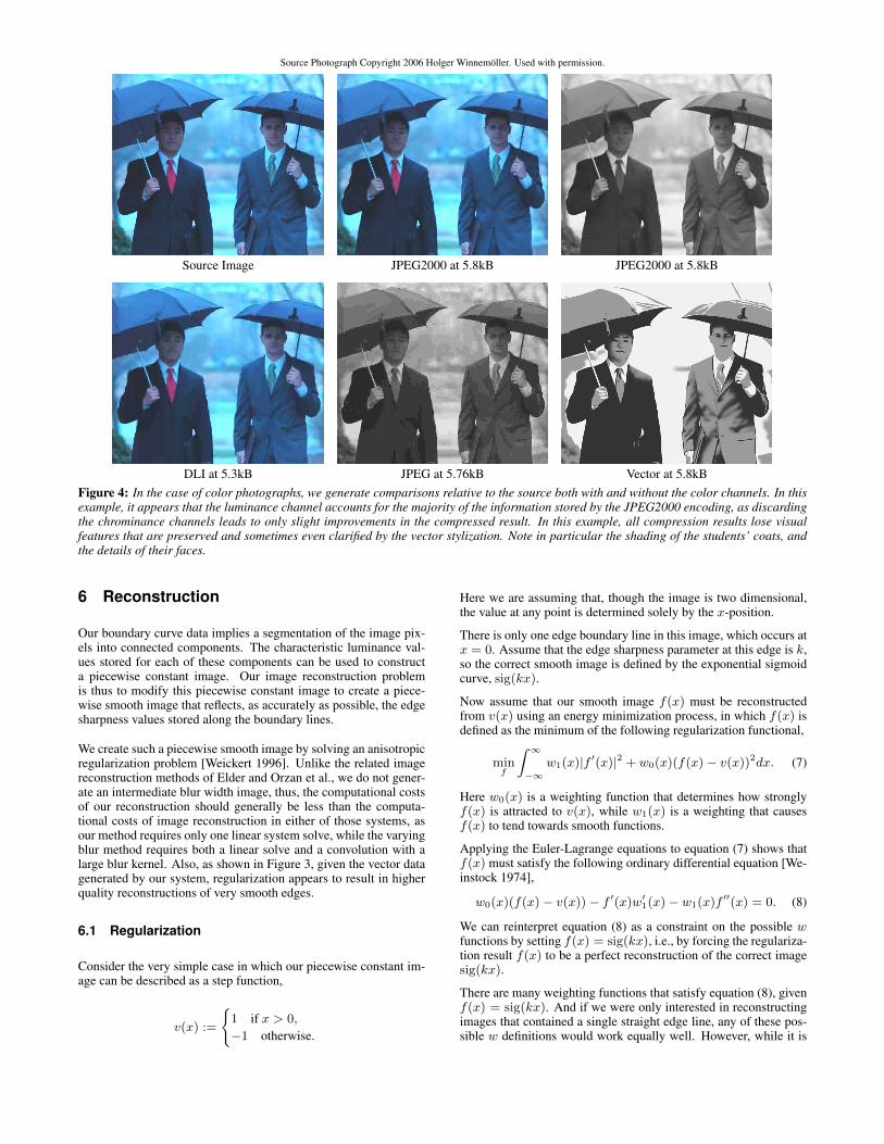
DLI at 5.3kB JPEG at 5.76kB Vector at 5.8kBFigure 4: In the case of color photographs, we generate comparisons relative to the source both with and without the color channels. In thisexample, it appears that the luminance channel accounts for the majority of the information stored by the JPEG2000 encoding, as discardingthe chrominance channels leads to only slight improvements in the compressed result. In this example, all compression results lose visualfeatures that are preserved and sometimes even clarified by the vector stylization. Note in particular the shading of the students’ coats, andthe details of their faces.

6 Reconstruction

Our boundary curve data implies a segmentation of the image pix-els into connected components. The characteristic luminance val-ues stored for each of these components can be used to constructa piecewise constant image. Our image reconstruction problemis thus to modify this piecewise constant image to create a piece-wise smooth image that reflects, as accurately as possible, the edgesharpness values stored along the boundary lines.

We create such a piecewise smooth image by solving an anisotropicregularization problem [Weickert 1996]. Unlike the related imagereconstruction methods of Elder and Orzan et al., we do not gener-ate an intermediate blur width image, thus, the computational costsof our reconstruction should generally be less than the computa-tional costs of image reconstruction in either of those systems, asour method requires only one linear system solve, while the varyingblur method requires both a linear solve and a convolution with alarge blur kernel. Also, as shown in Figure 3, given the vector datagenerated by our system, regularization appears to result in higherquality reconstructions of very smooth edges.

6.1 Regularization

Consider the very simple case in which our piecewise constant im-age can be described as a step function,

v(x) :=

1 if x > 0,

−1 otherwise.

Here we are assuming that, though the image is two dimensional,the value at any point is determined solely by the x-position.

There is only one edge boundary line in this image, which occurs atx = 0. Assume that the edge sharpness parameter at this edge is k,so the correct smooth image is defined by the exponential sigmoidcurve, sig(kx).

Now assume that our smooth image f(x) must be reconstructedfrom v(x) using an energy minimization process, in which f(x) isdefined as the minimum of the following regularization functional,

minf

∫ ∞−∞

w1(x)|f ′(x)|2 + w0(x)(f(x)− v(x))2dx. (7)

Here w0(x) is a weighting function that determines how stronglyf(x) is attracted to v(x), while w1(x) is a weighting that causesf(x) to tend towards smooth functions.

Applying the Euler-Lagrange equations to equation (7) shows thatf(x) must satisfy the following ordinary differential equation [We-instock 1974],

w0(x)(f(x)− v(x))− f ′(x)w′1(x)− w1(x)f ′′(x) = 0. (8)

We can reinterpret equation (8) as a constraint on the possible wfunctions by setting f(x) = sig(kx), i.e., by forcing the regulariza-tion result f(x) to be a perfect reconstruction of the correct imagesig(kx).

There are many weighting functions that satisfy equation (8), givenf(x) = sig(kx). And if we were only interested in reconstructingimages that contained a single straight edge line, any of these pos-sible w definitions would work equally well. However, while it is

Uncompressed Stylization Vector at 2.1kB Stylization at 2.1kB

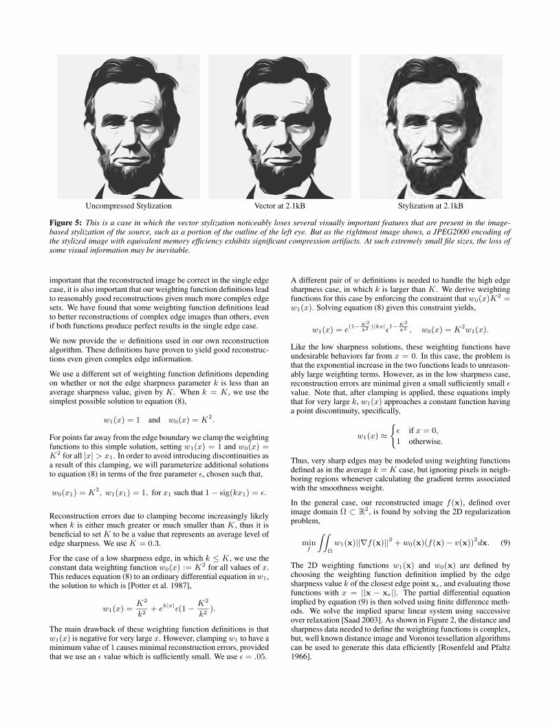
Figure 5: This is a case in which the vector stylization noticeably loses several visually important features that are present in the image-based stylization of the source, such as a portion of the outline of the left eye. But as the rightmost image shows, a JPEG2000 encoding ofthe stylized image with equivalent memory efficiency exhibits significant compression artifacts. At such extremely small file sizes, the loss ofsome visual information may be inevitable.

important that the reconstructed image be correct in the single edgecase, it is also important that our weighting function definitions leadto reasonably good reconstructions given much more complex edgesets. We have found that some weighting function definitions leadto better reconstructions of complex edge images than others, evenif both functions produce perfect results in the single edge case.

We now provide the w definitions used in our own reconstructionalgorithm. These definitions have proven to yield good reconstruc-tions even given complex edge information.

We use a different set of weighting function definitions dependingon whether or not the edge sharpness parameter k is less than anaverage sharpness value, given by K. When k = K, we use thesimplest possible solution to equation (8),

w1(x) = 1 and w0(x) = K2.

For points far away from the edge boundary we clamp the weightingfunctions to this simple solution, setting w1(x) = 1 and w0(x) =K2 for all |x| > x1. In order to avoid introducing discontinuities asa result of this clamping, we will parameterize additional solutionsto equation (8) in terms of the free parameter ε, chosen such that,

w0(x1) = K2, w1(x1) = 1, for x1 such that 1− sig(kx1) = ε.

Reconstruction errors due to clamping become increasingly likelywhen k is either much greater or much smaller than K, thus it isbeneficial to set K to be a value that represents an average level ofedge sharpness. We use K = 0.3.

For the case of a low sharpness edge, in which k ≤ K, we use theconstant data weighting function w0(x) := K2 for all values of x.This reduces equation (8) to an ordinary differential equation inw1,the solution to which is [Potter et al. 1987],

w1(x) =K2

k2+ ek|x|ε(1− K2

k2).

The main drawback of these weighting function definitions is thatw1(x) is negative for very large x. However, clampingw1 to have aminimum value of 1 causes minimal reconstruction errors, providedthat we use an ε value which is sufficiently small. We use ε = .05.

A different pair of w definitions is needed to handle the high edgesharpness case, in which k is larger than K. We derive weightingfunctions for this case by enforcing the constraint that w0(x)K2 =w1(x). Solving equation (8) given this constraint yields,

w1(x) = e(1−K2

k2 )|kx|ε1−K2

k2 , w0(x) = K2w1(x).

Like the low sharpness solutions, these weighting functions haveundesirable behaviors far from x = 0. In this case, the problem isthat the exponential increase in the two functions leads to unreason-ably large weighting terms. However, as in the low sharpness case,reconstruction errors are minimal given a small sufficiently small εvalue. Note that, after clamping is applied, these equations implythat for very large k, w1(x) approaches a constant function havinga point discontinuity, specifically,

w1(x) ≈

ε if x = 0,

1 otherwise.

Thus, very sharp edges may be modeled using weighting functionsdefined as in the average k = K case, but ignoring pixels in neigh-boring regions whenever calculating the gradient terms associatedwith the smoothness weight.

In the general case, our reconstructed image f(x), defined overimage domain Ω ⊂ R2, is found by solving the 2D regularizationproblem,

minf

∫∫Ω

w1(x)||∇f(x)||2 + w0(x)(f(x)− v(x))2dx. (9)

The 2D weighting functions w1(x) and w0(x) are defined bychoosing the weighting function definition implied by the edgesharpness value k of the closest edge point xe, and evaluating thosefunctions with x = ||x − xe||. The partial differential equationimplied by equation (9) is then solved using finite difference meth-ods. We solve the implied sparse linear system using successiveover relaxation [Saad 2003]. As shown in Figure 2, the distance andsharpness data needed to define the weighting functions is complex,but, well known distance image and Voronoi tessellation algorithmscan be used to generate this data efficiently [Rosenfeld and Pfaltz1966].

6.2 Post Smoothing

The image reconstructions generated by the regularization solvetend to accurately reproduce any smooth shading in the source styl-ized image. However, hard edges often suffer from “jaggies”, alias-ing artifacts that result from the conversion of the boundary data toa discrete image grid. One simple way to eliminate such artifacts isto reconstruct images at a much higher resolution than they will bedisplayed, and then downsample the results, thus taking advantageof the resolution independent nature of the data. However, we havefound it both more computationally efficient and more effective toapply a slight smoothing effect to the result. We use an anisotropicsmoother for this purpose, specifically, we apply coherence enhanc-ing anisotropic diffusion, as defined by Weickert [1996], using thecoherence biasing parameter α = .001, and scalespace parametert = 3.6.

7 Results

Our system is implemented in a mixture of Matlab and C. The dom-inant cost of image stylization and tracing is the line integral con-volution step, which can can require more than a second of pro-cessing time per image. Studies performed by Kyprianidis andDollner, however, demonstrate that similar convolutions can be per-formed at much greater speeds using GPU processing [Kyprianidisand Dollner 2008].

Reconstructing images at megapixel resolution takes several sec-onds, the overwhelming majority of which is spent performing thelinear solve. We use a combination of supersampling and postsmoothing to reduce aliasing artifacts in our result images, there-fore, all results are rendered at at least 1.5x the desired resolution.Again, the costs of image reconstruction could likely be dramat-ically reduced by using an iterative linear solver implemented inCUDA or OpenCL.

There are several cases in which our algorithms fail to create sim-ple, curve-based representations of an initial image. If the styliza-tion filter does not create a useful abstraction of the initial image,then our vectorization will also fail to be useful. Such failure casesoften appear to be over-blurred or over simplified. Additionally, ap-plying aggressive line simplification and region elimination settingscan lead to shape distortions in the vectorized results. While errorsof this last form can be fixed by using more conservative line sim-plification settings, doing so will increase curve complexity, lead-ing to results which fail in our goal of creating a vector graphic thatrepresents a simplification of the input photograph, in the sense ofimproved memory efficiency.

7.1 Memory Efficiency

Our goal is to create simple, stylized images in which the key visualcontent of a source image has been clarified, rather than discarded.Given an input photograph and the resulting vector image, the de-gree to which we are successful in this goal is difficult to quantify.

For example, consider a system in which, for any input photo-graph, the “vector stylization” returned is always an arrangementof two black boxes on a white background. From a memory effi-ciency standpoint, it is clear that a dramatic simplification has beenachieved. However, such a system could not reasonably claim to“preserve and clarify” the key visual content of the photograph.But, while quantifying the degree to which the stylizations are“good abstractions” is difficult, and, perhaps necessarily subjec-tive, identifying cases in which the vectorizations fail to improvememory efficiency is straightforward.

Source Image at 1.28kB Vector at 1.28kB

Figure 6: Simplification relative to a lossy compression of the inputphotograph, as generated by the Kadaku JPEG2000 encoder.

7.1.1 Simplification Relative to the Input Photograph

If the vector data, when stored to disk, has a higher encoding costthan a high fidelity compression of the input photograph, then theclaim that the vector stylization is an effective simplification is sus-pect. For example, even if the vector image appears visually simplerthan the source photograph, if the initial photograph can be encodedwith a high degree of visual fidelity using 7kB, then any vector re-sult that requires more than 7kB of storage space has actually madethe source data more complex than it was in its original form.

The resolution independent nature of our vector format makes di-rect comparisons of encoding efficiency impossible. As our vectordata can be used to reconstruct smooth images at arbitrarily largesizes, storage efficiency per-pixel of output data is undefined.

Thus, for a collection of example vector stylizations, we have cre-ated compressed versions of the input photographs having similarfilesizes. Cases in which the compressed images suffer from min-imal visual distortions must be considered failure cases for our al-gorithm, in the sense that the generated vector data does not appearto represent a true simplification of the input photograph.

For the purposes of these tests, we have used the KakaduJPEG2000 encoder to create lossy compression results at variousfile sizes [Taubman 2010]. The Kakadu encoder is arguably themost efficient JPEG2000 encoder available. It performed very wellin the 2005 codec comparison studies performed at MSU [Vatolinet al. 2005]. More recently, it proved to be the best of the vari-ous JPEG2000 codecs tested by Lee in his DLI performance stud-ies [Lee 2010].

We have also generated a few results relative to the older JPEGimage compression standard. In these cases our vector images typ-ically pass the data simplification test easily, as JPEG compressionshows strong blocking artifacts at filesizes close to those of our vec-tor encodings. The JPEG result shown in Figure 4 was generatedusing XnView’s optimized Huffman table encoder.

Using JPEG2000 compression results in less extreme visual errors,but noticeable artifacts frequently still result when images are com-pressed into file sizes that match those achieved by our vector for-mat.

Finally, in some of the Figures in this paper, we have included com-parisons relative to the DLI research codec. As of 2009, DLI wasthe record holder for minimum MSE compression of image data atvery small file sizes [Lee 2010]. But the DLI research codec doesnot allow files to be created as a specified bitrate, so generatingcomparison images matching specific file sizes is difficult.

Comparing the JPEG result shown in Figure 4 to the DLI or

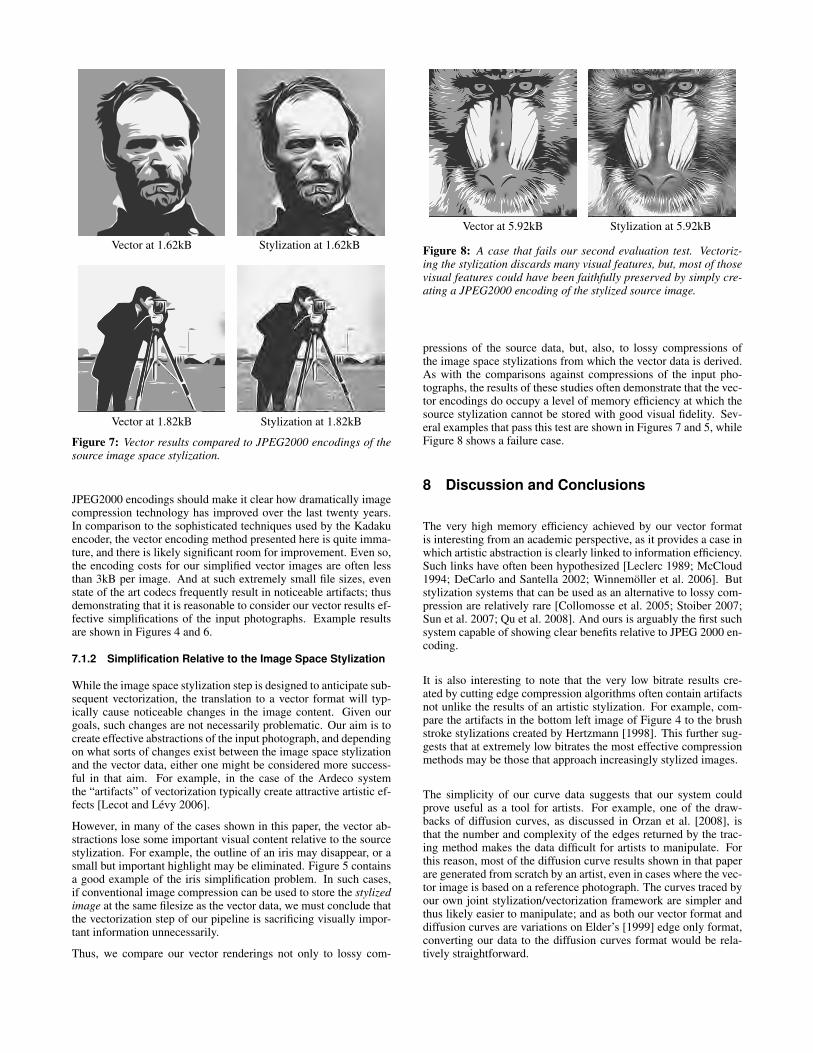
Vector at 1.62kB Stylization at 1.62kB

Vector at 1.82kB Stylization at 1.82kB

Figure 7: Vector results compared to JPEG2000 encodings of thesource image space stylization.

JPEG2000 encodings should make it clear how dramatically imagecompression technology has improved over the last twenty years.In comparison to the sophisticated techniques used by the Kadakuencoder, the vector encoding method presented here is quite imma-ture, and there is likely significant room for improvement. Even so,the encoding costs for our simplified vector images are often lessthan 3kB per image. And at such extremely small file sizes, evenstate of the art codecs frequently result in noticeable artifacts; thusdemonstrating that it is reasonable to consider our vector results ef-fective simplifications of the input photographs. Example resultsare shown in Figures 4 and 6.

7.1.2 Simplification Relative to the Image Space Stylization

While the image space stylization step is designed to anticipate sub-sequent vectorization, the translation to a vector format will typ-ically cause noticeable changes in the image content. Given ourgoals, such changes are not necessarily problematic. Our aim is tocreate effective abstractions of the input photograph, and dependingon what sorts of changes exist between the image space stylizationand the vector data, either one might be considered more success-ful in that aim. For example, in the case of the Ardeco systemthe “artifacts” of vectorization typically create attractive artistic ef-fects [Lecot and Levy 2006].

However, in many of the cases shown in this paper, the vector ab-stractions lose some important visual content relative to the sourcestylization. For example, the outline of an iris may disappear, or asmall but important highlight may be eliminated. Figure 5 containsa good example of the iris simplification problem. In such cases,if conventional image compression can be used to store the stylizedimage at the same filesize as the vector data, we must conclude thatthe vectorization step of our pipeline is sacrificing visually impor-tant information unnecessarily.

Thus, we compare our vector renderings not only to lossy com-

Vector at 5.92kB Stylization at 5.92kB

Figure 8: A case that fails our second evaluation test. Vectoriz-ing the stylization discards many visual features, but, most of thosevisual features could have been faithfully preserved by simply cre-ating a JPEG2000 encoding of the stylized source image.

pressions of the source data, but, also, to lossy compressions ofthe image space stylizations from which the vector data is derived.As with the comparisons against compressions of the input pho-tographs, the results of these studies often demonstrate that the vec-tor encodings do occupy a level of memory efficiency at which thesource stylization cannot be stored with good visual fidelity. Sev-eral examples that pass this test are shown in Figures 7 and 5, whileFigure 8 shows a failure case.

8 Discussion and Conclusions

The very high memory efficiency achieved by our vector formatis interesting from an academic perspective, as it provides a case inwhich artistic abstraction is clearly linked to information efficiency.Such links have often been hypothesized [Leclerc 1989; McCloud1994; DeCarlo and Santella 2002; Winnemoller et al. 2006]. Butstylization systems that can be used as an alternative to lossy com-pression are relatively rare [Collomosse et al. 2005; Stoiber 2007;Sun et al. 2007; Qu et al. 2008]. And ours is arguably the first suchsystem capable of showing clear benefits relative to JPEG 2000 en-coding.

It is also interesting to note that the very low bitrate results cre-ated by cutting edge compression algorithms often contain artifactsnot unlike the results of an artistic stylization. For example, com-pare the artifacts in the bottom left image of Figure 4 to the brushstroke stylizations created by Hertzmann [1998]. This further sug-gests that at extremely low bitrates the most effective compressionmethods may be those that approach increasingly stylized images.

The simplicity of our curve data suggests that our system couldprove useful as a tool for artists. For example, one of the draw-backs of diffusion curves, as discussed in Orzan et al. [2008], isthat the number and complexity of the edges returned by the trac-ing method makes the data difficult for artists to manipulate. Forthis reason, most of the diffusion curve results shown in that paperare generated from scratch by an artist, even in cases where the vec-tor image is based on a reference photograph. The curves traced byour own joint stylization/vectorization framework are simpler andthus likely easier to manipulate; and as both our vector format anddiffusion curves are variations on Elder’s [1999] edge only format,converting our data to the diffusion curves format would be rela-tively straightforward.

References

CABRAL, B., AND LEEDOM, L. C. 1993. Imaging vector fieldsusing line integral convolution. In SIGGRAPH ’93: Proceed-ings of the 20th annual conference on Computer graphics andinteractive techniques, ACM, New York, NY, USA, 263–270.

COLLOMOSSE, J. P., ROWNTREE, D., AND HALL, P. M. 2005.Stroke surfaces: Temporally coherent artistic animations fromvideo. IEEE Transactions on Visualization and ComputerGraphics 11, 5, 540–549.

DECARLO, D., AND SANTELLA, A. 2002. Stylization and ab-straction of photographs. In Proceedings of SIGGRAPH ’02,769–776.

EDWARDS, B. 1979. Drawing on the right side of the brain. J. P.Tarcher, Los Angeles, California, USA.

ELDER, J. H. 1999. Are edges incomplete? Int. J. Comput. Vision34, 2-3, 97–122.

GOOCH, B., REINHARD, E., AND GOOCH, A. 2004. Human fa-cial illustrations: Creation and psychophysical evaluation. ACMTrans. Graph. 23, 1, 27–44.

GRAHAM, R. L., KNUTH, D. E., AND PATASHNIK, O. 1994.Concrete Mathematics: A Foundation for Computer Science.Addison-Wesley Longman Publishing Co., Inc., Boston, MA,USA.

HERTZMANN, A. 1998. Painterly rendering with curved brushstrokes of multiple sizes. In SIGGRAPH ’98: Proceedings of the25th annual conference on Computer graphics and interactivetechniques, ACM, New York, NY, USA, 453–460.

KANG, H., LEE, S., AND CHUI, C. K. 2007. Coherent line draw-ing. In NPAR ’07: Proceedings of the 5th international sym-posium on Non-photorealistic animation and rendering, ACM,New York, NY, USA, 43–50.

KYPRIANIDIS, J. E., AND DOLLNER, J. 2008. Image abstrac-tion by structure adaptive filtering. In Proc. EG UK Theory andPractice of Computer Graphics, 51–58.

LECLERC, Y. G. 1989. Constructing simple stable descriptions forimage partitioning. International Journal of Computer Vision 3,1, 73–102.

LECOT, G., AND LEVY, B. 2006. Ardeco: Automatic region detec-tion and conversion. In Eurographics Symposium on Rendering.

LEE, D., 2010. DLI image compression .http://sites.google.com/site/dlimagecomp/software.

MAINBERGER, M., BRUHN, A., WEICKERT, J., AND FORCH-HAMMER, S. 2010. Edge-based compression of cartoon-like im-ages with homogeneous diffusion. Pattern Recognition In Press,Corrected Proof .

MCCLOUD, S. 1994. Understanding Comics. HarperCollins.

MUMFORD, D., AND SHAH, J. 1989. Optimal approximationsby piecewise smooth functions and associated variational prob-lems. Communications on Pure and Applied Mathematics 42,577–685.

ORZAN, A., BOUSSEAU, A., WINNEMOLLER, H., BARLA, P.,THOLLOT, J., AND SALESIN, D. 2008. Diffusion curves: avector representation for smooth-shaded images. In SIGGRAPH’08: ACM SIGGRAPH 2008 papers, ACM, New York, NY,USA, 1–8.

POTTER, M. C., GOLDBERG, J. L., AND POTTER, M. C. 1987.Mathematical methods / Merle C. Potter, Jack Goldberg, 2nded. ed. Prentice-Hall, Englewood Cliffs, N.J. :.

PRICE, B., AND BARRETT, W. 2006. Object-based vectorizationfor interactive image editing. Vis. Comput. 22, 9, 661–670.

QU, Y., PANG, W.-M., WONG, T.-T., AND HENG, P.-A. 2008.Richness-preserving manga screening. ACM Transactions onGraphics (SIGGRAPH Asia 2008 issue) 27, 5 (December),155:1–155:8.

ROSENFELD, A., AND PFALTZ, J. L. 1966. Sequential operationsin digital picture processing. J. ACM 13, 4, 471–494.

SAAD, Y. 2003. Iterative Methods for Sparse Linear Systems,second ed. SIAM, Philadelphia.

SELINGER, P., 2003. Potrace: a polygon-based tracing algorithm.http://potrace.sourceforge.net/potrace.pdf, September.

STOIBER, N. 2007. Compression of images and videos by ge-ometrization. Master’s thesis, Technische Universitat Munchen.

SUN, J., LIANG, L., WEN, F., AND SHUM, H.-Y. 2007. Im-age vectorization using optimized gradient meshes. ACM Trans.Graph. 26, 3, 11.

TAUBMAN, D., 2010. Kakadu JPEG2000 Encoder. University ofNew South Wales. http://www.kakadusoftware.com/.

VATOLIN, D., MOSKVIN, A., PETROV, O., ANDTITARENKO, A., 2005. JPEG 2000 image codecs com-parison. Moscow State University. http://compression.ru/video/codec comparison/jpeg2000 codecs comparison en.html.

WEICKERT, J. 1996. Anisotropic diffusion in image processing.PhD thesis, Dept. of Mathematics, University of Kaiserslautern.

WEINSTOCK, R. 1974. Calculus of Variations: With Applicationsto Physics and Engineering. Dover Pub. Inc., New York.

WINNEMOLLER, H., OLSEN, S. C., AND GOOCH, B. 2006. Real-time video abstraction. ACM Trans. Graph. 25, 3, 1221–1226.

XIA, T., LIAO, B., AND YU, Y. 2009. Patch-based image vec-torization with automatic curvilinear feature alignment. ACMTrans. Graph. 28, 5, 1–10.