Embed Size (px)
Citation preview
Boillod-Cerneux France WS 2010/2011
GPU - PETSc for neutron transport equation
partnerships:

ThanksThanksI thank G. Haase for to help for the outcome of my project, and backing me in my work
during the all semester.
OutlinesOutlines
Introduction page 5
0. CEA page 6
I. Presentation of neutron transport equation page 71.1 Context page 71.2 Neutron transport equation page 81.3 Neutron diffusion equation page 8
II. The linear system to solve page 10
2.1 Discretization of neutron diffusion equation page 10
2.2 Domain decomposition page 12
2.3 The linear system page 132.4 The MINOS solver page 142.5 The linear system used for our project page 15
III Introduction to KSP PETSc methods page 163.1 The numerical methods page 16
IV Introduction to Multigrid with PETSc page 174.1 The Multigrid concept page 174.2 Multigrid with PETSc page 18
V PETSc-CUDA presentation page 205.1 PETSc with CUDA page 20
VI PETSc used in neutronic domain page 21
6.1 Multigrid code page 216.2 Multigrid Results page 246.3 KSP code page 336.4 KSP Results page 36
VII GPU used in neutronic domain page 447.1 Introduction page 447.2 Conjugate gradient with CUDA-CPU page 467.3 Conjugate gradient with Cublas page 477.4 Results page 48
Conclusion page 55Bibliography page 56Webography page 56
Abstract. This paper is about the optimisation for solving the neutron transport equation. We are looking for to implement the conjugate gradient method with GPU programmation, in order to speed-up the resolution of neutron transport equation. We will study different implementations of conjugate-gradient, with CUDA and CUBLAS langage, and also with PETSc-CUDA. Then, we will discuss on multigrid implementation with PETSc, and finally conclude on obtained perfomances.
Key words. Parallel Computing, Eigenproblem, Conjugate-gradient method, multigrid, Graphics Programmation Unit
IntroductionIntroductionAs computer power increases, scientists want to solve more and more complicated
problems. They need to optimize both memory requirements and time computation, which is commonly called « High Performance Computing ».
HPC is applied to sciences as well as business or data mining and holds a leading place in every domain which uses computer science. More than a concept, HPC is nowadays a standard and is used in several domains, like petrology, sismology, economy, nuclear …
Many codes developped 10 or 15 years ago need to be rewritten in order to take advantage of parallel computers. This is the case of MINOS, a CEA neutronics code. MINOS'target is to solve the neutron transport equation in order to compute the power produced by a power plant.
Indeed, the control of nuclear reaction is based on the neutron transport equation, that's why its resolution is a major purpose.
Moreover, the computation time is essential, so as to intervene fast to reduce or to improve a nuclear reaction, in terms of the needs energy.
Although MINOS is considerably optimised, CEA is still doing research to ameliorate it. The recent researchs about GPU programmation prove that using graphic cards to make a part of calculations can considerably speed-up the time calculation. It exists differents langages in order to program on graphic cards, such that CUDA or CUBLAS. As the performances of GPU are really satisfying, some libraries and langages such as PETSc or Python are working on improve their perfomance by using GPU programmation. PETSc is a free library which is very adapted to factorize and solve linear system using parallelism. Indeed, PETSc uses MPI or openMPI and offers a lot of functions for linear and non linear systems.
The subject of this project is to implement the conjugate-gradient method with several langages using GPU programmation, in order to use it later for solving the neutron transport equation in one dimension, as in this case, the matrix is symmetric and positiv-definite. We will use the langages CUDA, CUBLAS, and the PETSc library with CUDA, as it extends a lot of numerical methods to solve linear systems, notably several version of conjugate-gradient method.
The organization of this paper is as follows. First, we will present the neutron transport equation, and then explain how we obtain from this equation a linear system. We will focus next on the generated codes for conjugate-gradient methode, and their structure. We will then discuss on multigrid programmation with PETSC. Finally, we will study the performances we obtain, and conclude on it.

0. CEABased in Ile-de-France, CEA Saclay is a national and european research center. CEA
gathers applied research as well as fundamental research. With 5000 researchers, CEA Saclay contributes to improve nuclear central park optimization, but also its functionment and does research to manage nuclear garbages, respecting the environment. To do so, CEA bases its research on simulation, especially with computer science.
I. Presentation of neutron transport equationThe neutron transport equation is fundamental in neutronic science. Indeed, scientists must
solve it in order to understand the nuclear reaction in a core. In this part, we will present first the issue and then the neutron transport equation. We will end with the neutron diffusion equation, linked with the first mentioned equation.
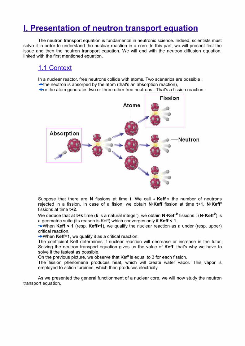
1.1 Context In a nuclear reactor, free neutrons collide with atoms. Two scenarios are possible :
the neutron is absorped by the atom (that's an absorption reaction),or the atom generates two or three other free neutrons : That's a fission reaction.
Suppose that there are N fissions at time t. We call « Keff » the number of neutrons rejected in a fission. In case of a fision, we obtain N∙Keff fission at time t+1, N∙Keff² fissions at time t+2. We deduce that at t+k time (k is a natural integer), we obtain N∙Keffk fissions : (N∙Keffk) is a geometric suite (its reason is Keff) which converges only if Keff < 1.
When Keff < 1 (resp. Keff>1), we qualify the nuclear reaction as a under (resp. upper) critical reaction.
When Keff=1, we qualify it as a critical reaction. The coefficient Keff determines if nuclear reaction will decrease or increase in the futur. Solving the neutron transport equation gives us the value of Keff, that's why we have to solve it the fastest as possible.On the previous picture, we observe that Keff is equal to 3 for each fission.The fission phenomena produces heat, which will create water vapor. This vapor is employed to action turbines, which then produces electricity.
As we presented the general functionment of a nuclear core, we will now study the neutron transport equation.
1.2 Neutron transport equation
The neutron transport equation has been established by L. Boltzman in 1872, and is also called Boltzmann's equation¹. We present it presented as follows :
¹
¹ Reference : Précis de neutronique Paul REUSSWhere :
Φ is the neutron flux (mol/m³),the current is (mol/m²sec).
This equation cannot be solved with some particular conditions, for example, in case of stationary state of Fick's laws (etablished in 1855). Before introducing the Fick's law, let's see the diffusion definition : «a system tends to homogenize its chemical elements concentrations : this natural phenomena is called diffusion.»
First Fick's law: it relates the diffusive flux to the concentration field, by postulating that the flux goes from regions of high concentration to regions of low concentration. The magnitude of flux is proportional to the concentration gradient. In one dimension, we obtain this equation:
Where:
D is the diffusion coefficient (m²/sec).
Second Fick's law: it predicts how diffusion causes the concentration field to change with time. It is represented with this equation:
Where:
x is the position.
The use of Fick's law in a core reactor leads to the diffusion approximation: Boltzmann's equation can be simplify and aproximate by the neutron diffusion equation.
We will now focus on this equation, which depends upon 7 variables only.
1.3 Neutron diffusion equationWe saw previously the diffusion definition: To illustrate this definition with neutrons exemple, that's means that in a core, the dense neutrons area tends to populate the sparse neutron areas. In the neutron diffusion equation, we introduce a new variable : Where:
p is the current.The neutron diffusion equation is as follows:Where: ²
Sφ are the scattering sources,Sf are the fission sources,R is the domain,σa is the absorption coefficient,σf is the fission coefficient,λ is Keff.
² Reference : Pierre Guérin thesis

In fact, this equation doesn't consider the angular variable.
Now we have presented the neutron diffusion equation, and justify its utility, we will focus on the corresponding linear system. Indeed, it is more adapted to use the linear system because of the large panel of numerical methods that can solve the equation.

II. The linear system to solve
In this part, we will present the method used to discretize the equation diffusion, and the decomposition domain method. Then we will explain the obtained linear system and finally, we will present the solver MINOS, the CEA's program to modelize the resolution of linear system.
2.1 Discretization of neutron diffusion equation
Let's consider the previous neutron diffusion equation¹ :
(1.1)
(1.2)
(1.3)
These coupled equations are discretized with Raviart Thomas with Finite elements method. There, we will detail how to obtain the linear system from these equations.We consider:
and satisfying the neutron diffusion equation.Let multiply the first equation line by a vector q, and the second with a function φ (φ is a squared-integrable function). We write this system with its variational form, in order to discretize the set of equation (1.1) and (1.3) with a finite element method. We finally obtain the following system :
(2.1)
(2.2)
(2.3)
We now apply the Green's formula on equation (2.1):
(3.1)
(3.2)
(3.3)
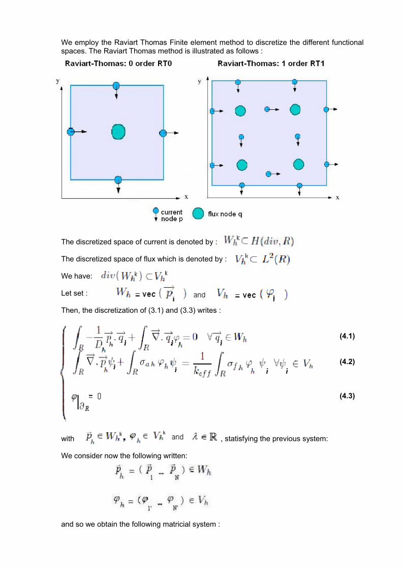
We employ the Raviart Thomas Finite element method to discretize the different functional spaces. The Raviart Thomas method is illustrated as follows :
The discretized space of current is denoted by :
The discretized space of flux which is denoted by :
We have:
Let set :
Then, the discretization of (3.1) and (3.3) writes :
(4.1)
(4.2)
(4.3)
with , statisfying the previous system:
We consider now the following written:
and so we obtain the following matricial system :
Bφ – AP = 0Tφ – BTP = S
with :
This system can be rewritten with P as single unknwon member :
φ = T -1 ( S – BT P) and replace the new epression of φ in the previous matrix system : (BT -1BT + A)P = BT -1S
The biggest eigen value of this linear system is
In the Raviart Thomas case, px and py are uncoupled and the system writes :
B = Bx + By A = | Ax - || - Ay |
We fix: Wx = Ax + BxTx -1BxT and Wy = Ay + ByTy -1ByT
Finally, we obtain the following linear system : Wx BxTx -1ByT
ByTy -1BxT Wy
To solve this linear system, CEA currently factorizes the previous matrix with Cholesky method, and solve it with a Gauss Seidel per blocs.
In our specific case, the domain decomposition method is used too to solve more precisely the diffusion equation.
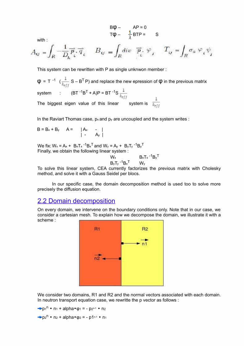
2.2 Domain decompositionOn every domain, we intervene on the boundary conditions only. Note that in our case, we consider a cartesian mesh. To explain how we decompose the domain, we illustrate it with a scheme :
We consider two domains, R1 and R2 and the normal vectors associated with each domain. In neutron transport equation case, we rewritte the p vector as follows :
p1n • n1 + alpha•φ1 = - p2n-1 • n2
p2n • n2 + alpha•φ2 = - p1n-1 • n1
and introduce this it in the following system :
(5.1)
(5.2)
With the same operations detailed in the previous paragraph, the linear system which is very similar as the one mentioned before. Indeed, this decomposition domain method is an iterative one : in consequence, only the second member of the system is modify.
All the previous operations contributes to give a linear system, which form is Ax = b. It is easier to solve this kind of system, because we dispose of a lot of numerical methods to solve it.In the next paragraph, we will focus on the obtained linear system, which returns the coefficient Keff.
2.3 The linear system
The following linear system1 is the result of the decomposition domain and discretization method application, realised on equation in neutron diffusion. This system is a sequential linear system.
Ax + BxTx -1BxT BxTx -1ByT 1
ByTy -1BxT Ay + ByTy -1ByT
1Reference : Pierre guerin thesis
Caracteristics of matrices :H' is symmetric positiv defined, T is diagonal, but it depends on the choice of Wh and Vh
B is bidiagonal,A is a dense matrix (A is also called reference of coupling of currents matrix)W has the same profil as A,S is the second member.
It results that the biggest eigen value of this linear system is : to solve this linear system is a major issue for the control of a nuclear reaction.
Currently, CEA implements a Cholesky method to factorize the matrix H' and then, Gauss Seidel method to solve the linear system.
As the matrice size is huge, we use parallelization to implement the solver of this linear system. Particularly, the MINOS Solver is a parallelised code, developped in C++, which makes this resolution.
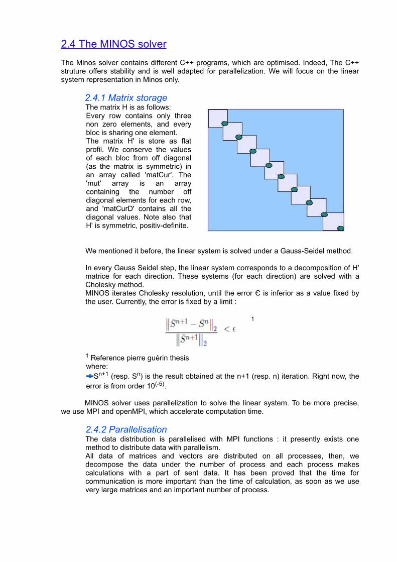
2.4 The MINOS solverThe Minos solver contains different C++ programs, which are optimised. Indeed, The C++ struture offers stability and is well adapted for parallelization. We will focus on the linear system representation in Minos only.
2.4.1 Matrix storageThe matrix H is as follows:Every row contains only three non zero elements, and every bloc is sharing one element.The matrix H' is store as flat profil. We conserve the values of each bloc from off diagonal (as the matrix is symmetric) in an array called 'matCur'. The 'mut' array is an array containing the number off diagonal elements for each row, and 'matCurD' contains all the diagonal values. Note also that H' is symmetric, positiv-definite.
We mentioned it before, the linear system is solved under a Gauss-Seidel method.
In every Gauss Seidel step, the linear system corresponds to a decomposition of H' matrice for each direction. These systems (for each direction) are solved with a Cholesky method.MINOS iterates Cholesky resolution, until the error Є is inferior as a value fixed by the user. Currently, the error is fixed by a limit :
1
1 Reference pierre guérin thesiswhere:
Sn+1 (resp. Sn) is the result obtained at the n+1 (resp. n) iteration. Right now, the error is from order 10(-5).
MINOS solver uses parallelization to solve the linear system. To be more precise, we use MPI and openMPI, which accelerate computation time.
2.4.2 ParallelisationThe data distribution is parallelised with MPI functions : it presently exists one method to distribute data with parallelism.All data of matrices and vectors are distributed on all processes, then, we decompose the data under the number of process and each process makes calculations with a part of sent data. It has been proved that the time for communication is more important than the time of calculation, as soon as we use very large matrices and an important number of process.

2.5 The linear system used for our projectAs I can not access to the exact CEA matrix and vectors, I choose to use an other
symmetric positive definite matrix. Moreover, the storage format of CEA matrix is not optimal, so we loose a considerable time to translate it as a PETSc storage format. In this case, we modify a litlle bit the matrix structure, and use a tridiagonal symmetric matrix.
That will be better to compare the time calculation, because the time to translate the matrix format will not interfer.
The aim of this project is to implement the conjugate-gradient method, in order to solve the linear system with it. We implement it by using graphic card programmation, so we can speed-up the time calculation. In what follows, we will briefly study the PETSc library, and detail all the KSP methods proposed to solve our linear system.
III Introduction to KSP PETSc methodsPETSc in an abreviation for «Portable, Extensible Toolkit for Scientific computation». This
library provides functions and many tools to implements numerical methods used to solve linear and non linear systems. PETSc is particularly adapted for sparse an dense systems as well as large-scale systems, because most of PETSc's functions are parallelized. In this paragraph, we will introduce the KSP application for solving linear systems.
3.1 The numerical methodsIn this part, we will present the diverse numerical methods we chose to solve our linear
system. We will first explain theoritically the different numerical methods which are developped.
The Conjugate Gradient methods :This method is an effective means to solve linear systems where the coefficient matrix is symmetric and positive definite.To begin, we consider a linear system like Ax = b, where A is symmetric and positive definite. We fixe a vector x(0) , and successively calculate x(1) , x(2) , x(3) ,..., x(k-1) to generate a sequence of {x(k)} to approximate the solution x of Ax = b. We decompose A as the followed format : A = L+D+L(t) where L is a strictly lower triangular matrix and D a diagonal matrix of the same size as L.We need next to calculate the matrix M, where M= (D+L)D(-1)(D+L)(t)We apply next the following algorithm : p(0) = r(0) = b – Ax(0)
Mr ' (0) = r(0)
until convergence, do : a(k) = (r(k) , r ' (k)) / (p(k) , Ap(k))x(k+1) = x(k) + a(k) p(k) r(k+1) = r(k) – a(k)Ap(k)
Mr ' (k+1)= r(k+1)
b(k) = (r(k+1) , r ' (k+1)) / (r(k) , r ' (k))p(k+1) = r ' (k+1) + b(k)p(k) = b – Ax(k+1)
we converge when p(k+1) = 0.This method corresponds to the KSP_TYPE « CG ».Conjugate Gradient Method on the Normal EquationsThe cgne solver applies too the CG iterative method, but it is applied to the normal equations without explicitely forming the matrix A(t)A.This method corresponds to the KSP_TYPE « CGNE ». As we saw, the KSP object in PETSc are particularly adapted to solve linear systems.
However, PETSc also developped the multigrid concept, as it is more and more used in HPC domain. PETSc offers a DMMG object, which creates multigrid, very adapted for linear or non linear systems. In what follows, we will study the DMMG concept with PETSc.
IV Introduction to Multigrid with PETScPETSc in an abreviation for «Portable, Extensible Toolkit for Scientific computation». This
library provides functions and many tools to implements numerical methods used to solve linear and non linear systems. PETSc is particularly adapted for sparse an dense systems as well as large-scale systems, because most of PETSc's functions are parallelized. In this paragraph, we will introduce the multigrid application for solving linear systems, and then explain how PETSc implements it.
4.1 The Multigrid conceptTo introduce the multigrid concept, we will consider the classic example: Poisson equation in 1 dimension.
-Δ u = f (1), on [0,1] (1.1)u(0) = u(1) = 0 (boundary conditions). (1.2)
We apply the finite difference method (second order) on (1.1), and then obtain the following linear system:
- u(i+1) + 2u(i) - u(i-1) = fi (2.1)h² (h is the grid size) (2.2)
h is generally 1/(n+1).With can rewritte these equation with a matrix form:
Au = f (3.1)
u = (u1, u2, … , uN-1)T (3.2)u(0) = u(N) = 0 (3.3)
f = (f1, f2, … , fN-1)T (3.4)The discretized form of equation (3.1) is as a linear system:
Ah uh = fh (4.1)Applying Jacobi or Gauss-Seidel algorithm on linear system like (3.1) determine the u vector solution, which has the following form:
u(i) = (u(i+1) + u(i-1) + h²fi) / 2 ; i=1, …, N (5.1)Note that the Gauss-Seidel method is like Jacobi one, by using for u(i+1) the previous calculated value (updated for each iteration), until we obtain the convergence. The system Au = f admitt an exact solution, u. We define the error as:
e = u – v (6.1)The best example to study the different frequency componant of error is to consider the Fourrier modes. They have been introduced as initial data for Gauss-Seidel iterationBy considering the Fourrier's mode for several frequencies, we can etablish the two following deductions:
The error of classic iterativ methods is smoothed for every iteration. By ddecomposing the error as a Fourrier serie, we conclude that the high frequencies for a mesh with gridsize h are better amortized than the lower one.
The error low frequencies on a fine mesh will be considered as high frequencies on a coarse mesh, and so being amortized with iterativ method.We illustrate the steps for multigrid resolution of Au = f:
We make several Gauss-Seidel resolutions of Ah uh = fh so we obtain a vector vh, which is an approximation of u on the finest grid (pre-smooth)
We calculate the associated residu rh = fh – Ah vh
We consider this residu on a coarser grid (with 2h as gridsize) by using a restriction operator R
We solve the following equation: A2h (u2h – v2h) = A2h e2h = r2h
We use a prolongation (or interpolation) operator on e2h on the finest grid to calculate eh We modify in consequence the approximation vh: vh = vh + eh
We make several iterations of Gauss-Seidel on Ah uh = fh, considering as initial solution: vh.
We will now focus our attention on the multigrid with PETSc, as PETSc offers methods to handle with it.
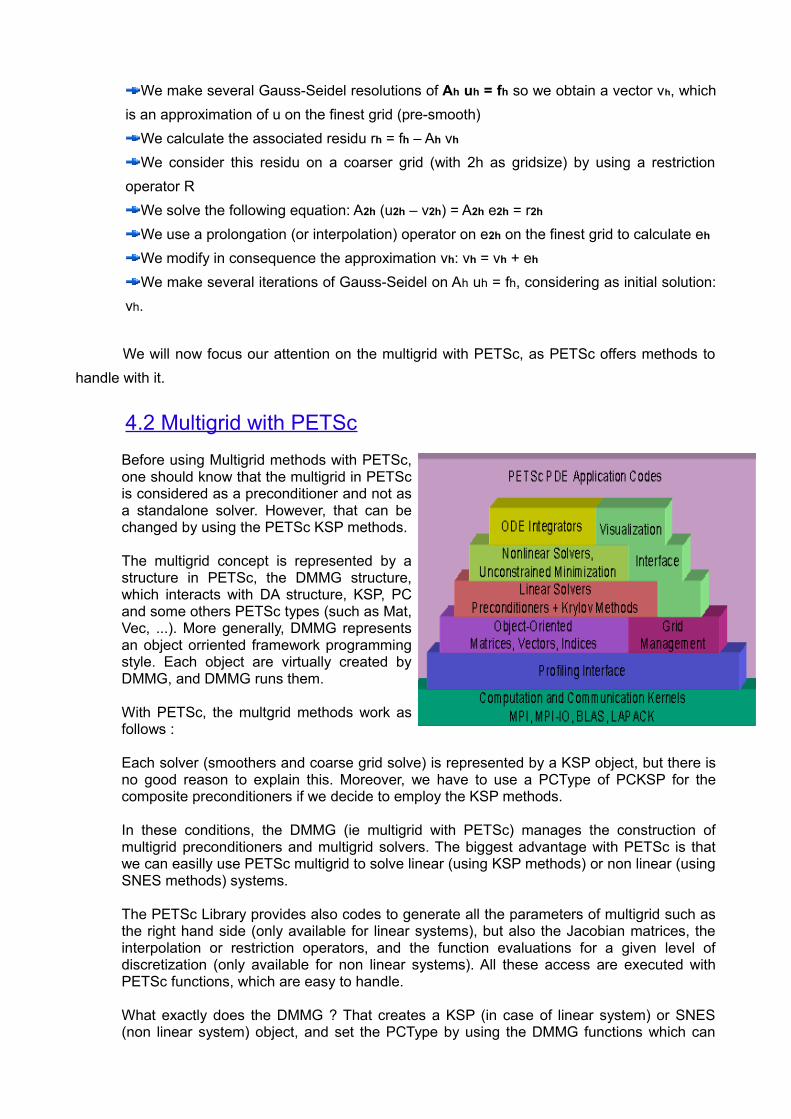
4.2 Multigrid with PETScBefore using Multigrid methods with PETSc, one should know that the multigrid in PETSc is considered as a preconditioner and not as a standalone solver. However, that can be changed by using the PETSc KSP methods.
The multigrid concept is represented by a structure in PETSc, the DMMG structure, which interacts with DA structure, KSP, PC and some others PETSc types (such as Mat, Vec, ...). More generally, DMMG represents an object orriented framework programming style. Each object are virtually created by DMMG, and DMMG runs them.
With PETSc, the multgrid methods work as follows :
Each solver (smoothers and coarse grid solve) is represented by a KSP object, but there is no good reason to explain this. Moreover, we have to use a PCType of PCKSP for the composite preconditioners if we decide to employ the KSP methods.
In these conditions, the DMMG (ie multigrid with PETSc) manages the construction of multigrid preconditioners and multigrid solvers. The biggest advantage with PETSc is that we can easilly use PETSc multigrid to solve linear (using KSP methods) or non linear (using SNES methods) systems.
The PETSc Library provides also codes to generate all the parameters of multigrid such as the right hand side (only available for linear systems), but also the Jacobian matrices, the interpolation or restriction operators, and the function evaluations for a given level of discretization (only available for non linear systems). All these access are executed with PETSc functions, which are easy to handle.
What exactly does the DMMG ? That creates a KSP (in case of linear system) or SNES (non linear system) object, and set the PCType by using the DMMG functions which can
access to PC associated to DMMG. For each level, the vectors, restriction (or interpolation) functions and the matrices are created and filled up. Note that, to introduce the values in initial solution, we use the DA structure (allows logically rectangular meshes creation in 1,2 or 3 dimensions). However, this one is not available with CUDA, it is replaced by DM one. The DM structure works as follows : That create a KSP or SNES object, then set the preconditioner type. The vectors, and restriction (or interpolation) functions, as well as the matrices are created and filled up for each level.
We will now explain how CUDA is used with the DMMG object.
V PETSc-CUDA presentationNowadays PETSc is available with CUDA. However, this version of PETSc is only available in petsc-dev, but will be included in the next PETSc version (3.2). The main advantage of PETSc is that the programmer does not haveto implement any CUDA's code: the programmation is still with PETSc functions, and CUDA appears only with the arguments when we run the code. This is still the same idea of PETSc, one code, but several runnings. The other advantage is that anyone can code on GPU, without deep knowledge about CUDA.
5.1 PETSc with CUDA
As the manipulation of CUDA with PETSc is really simple, the installation of PETSc-dev is still the most complicated part of work! One should consider, before installing the PETSc-dev version, which versions of cusp, thrust and CUDA are already installed on computer. Actually, the thrust version 1.4.0 and cusp 0.4.0 are available with PETSc-CUDA, which is a problem as it is complicated to find the good thrust version (there is no historic-versions on official website).The PETSc-dev version is currently installed on fermi, but there is still a problem of compatibility with the thrust versions. In consequence, I cannot run my KSP code with CUDA, as one of the necessary library to do so was'nt correctly installed.However, I could perfectly run my multigrid code: the DMMG object is particularly adapted for using CUDA. The main advantage of PETSc is that you have to implement your code, and then run it with the PETSc-CUDA options to use it : one code, but two way to run it, is the concept of PETSc-CUDA.Some operations are directly run on the GPU :
MatMult(...),KSPSolve(...),VecAXPY(...),VecWAYPX(...),as well as other vectors operations. Nowadays, we have to use the jacobi preconditioners if we want to run our code on GPU. Most of KSP types are also available with the GPU.
As we mentioned before, the programmer does not have to consider any CUDA implementation. We use the classic PETSc functions, and just run the code with the PETSc-CUDA options. For example, one should run a PETSc code with da_vec_type cuda if we want that the vector, associated to the DA/DMMG, runs on the GPU.
Now we studied the PETSc-CUDA, as well as CUDA behaviour with PETSc, let's see the different PETSc codes.
VI PETSc used in neutronic domainThe solver MINOS is currently parallelized to optimize the computation time. However,
PETSc offers functions which are parallelized : the user doesn't have to consider the MPI communication, which are optimized as well as the CUDA implementation. Besides, the storages format for matrices are optimized and adapted for such systems as neutron transport. We will present first the PETSc multigrid apply to a similar system as neutron transport equation (briefly presented in 2.5), then the codes using only KSP functions to solve the same system.
6.1 Multigrid codeWe implemented a program to solve the linear system (presented in 2.5) by using the DMMG functions. This is justify by the PETSc-CUDA implementation : as we said before, the DMMG options allow to run PETSc code on GPU.
The code is implemented as follows : void ksp_Results(KSP ksp) ; which returns the KSP results,void ksp_Options(KSP ksp) ; which inserts the differents options to the KSP,PetscErrorCode ComputeInitialSolution(DMMG dmmg) ; which compute the initial solution for DMMG,PetscErrorCode ComputeRHS_VecSet(DMMG dmmg,Vec b) ; which compute the right hand side for DMMG,PetscErrorCode ComputeMatrix_A(DMMG dmmg,Mat jac, Mat A) ; which compute the matrix associated to the DMMG.We won't detail void ksp_Results(KSP ksp) ; and void ksp_Options(KSP ksp) ; as they are similar as the KSP code presented in 4.4.
This function ComputeInitialSolution(DMMG dmmg) uses the DA structure to acces to the initial solution: in term of perfomance, this is much better. We insert the values to the vector by using a DA structure.
PetscErrorCode ComputeInitialSolution(DMMG dmmg) {DA da = (DA) dmmg->dm; PetscInt mx,xs,xm,i;PetscInt my,ys,ym,j; PetscScalar **array;
DAGetInfo(da, 0, &mx, &my, 0,0,0,0,0,0,0,0);DAGetCorners(da,&xs,&ys,0,&xm,&ym,0);Vec x = (Vec) dmmg->x;DAVecGetArray(da, x, &array);for (j=ys; j<ys+ym; j++){
for(i=xs; i<xs+xm; i++){array[j][i] = 1.0;
}}
DAVecRestoreArray(da, x, &array);VecAssemblyBegin(x);VecAssemblyEnd(x);return(0);
}
In the function ComputeRHS_VecSet(DMMG dmmg,Vec b), we use the VecSet(...) function, as it presents also good perfomances gain.PetscErrorCode ComputeRHS_VecSet(DMMG dmmg,Vec b) {PetscPrintf(PETSC_COMM_WORLD,"in rhs VecSet\n");
VecSet(b,1.0);VecAssemblyBegin(b);VecAssemblyEnd(b);return(0);
}
the function ComputeMatrix_A(DMMG dmmg,Mat jac, Mat A) insert the values in the matrix associated to the DMMG. We use MatSetValuesStencil, to insert all the values cause this function is particularly adapted for sparse matrix, and use the grid index.
PetscErrorCode ComputeMatrix_A(DMMG dmmg,Mat jac, Mat A) {
PetscInt m,n; MatStencil row, col[3];PetscScalar v[3]; DA da = (DA) dmmg->dm;PetscInt i,j,mx,my,xm,ym,xs,ys;
DAGetInfo(da, 0, &mx, &my, 0,0,0,0,0,0,0,0);DAGetCorners(da,&xs,&ys,0,&xm,&ym,0);for(i=xs; i<xs+xm; i++){
row.i=i;for (j=ys; j<ys+ym; j++){
row.j=j;if(i==xs){
v[0] = 1/(abs(i-j)+1.0);col[0].i = i; col[0].j = j;v[1] = 1/(abs(i-j)+1.0);col[1].i = i; col[1].j = j+1;MatSetValuesStencil(A,1,&row,2,col,v,INSERT_VALUES);
}else{if(j==ys){
v[0] = 1/(abs(i-j)+1.0);col[0].i = i; col[0].j = j;v[1] = 1/(abs(i-j)+1.0);col[1].i = i; col[1].j = j-1;MatSetValuesStencil(A,1,&row,2,col,v,INSERT_VALUES);
}else{if(j>=(i-1) && j<=(i+1)){
v[0] = 1/(abs(i-j)+1.0);col[0].i = i; col[0].j = j;v[1] = 1/(abs(i-j)+1.0);col[1].i = i; col[1].j = j-1;v[2] = 1/(abs(i-j)+1.0);col[2].i = i; col[2].j = j+1;MatSetValuesStencil(A,1,&row,3,col,v,INSERT_VALUES);
}}
}}
}MatAssemblyBegin(A,MAT_FINAL_ASSEMBLY);MatAssemblyEnd(A,MAT_FINAL_ASSEMBLY);return(0);
}
int main(int argc,char **argv) {
DMMG *dmmg; DA da;PetscReal norm; PC pc;
PetscInitialize(&argc,&argv,(char *)0,help);PetscOptionsSetFromOptions();DMMGCreate(PETSC_COMM_WORLD,1,PETSC_NULL,&dmmg);DMMGSetDM(dmmg,(DM)da);ComputeInitialSolution(*dmmg);DMMGSetKSP(dmmg,ComputeRHS_VecSet,ComputeMatrix_A);ksp_Options(DMMGGetKSP(dmmg));KSPGetPC(DMMGGetKSP(dmmg),&pc);PCSetType(pc,PCJACOBI);PCFactorSetShiftType(pc,MAT_SHIFT_POSITIVE_DEFINITE);
DMMGSetUp(dmmg);DMMGSolve(dmmg);VecAssemblyBegin(DMMGGetRHS(dmmg));VecAssemblyEnd(DMMGGetRHS(dmmg));ksp_Results(DMMGGetKSP(dmmg));VecAssemblyBegin(DMMGGetx(dmmg));VecAssemblyEnd(DMMGGetx(dmmg));DMMGView(dmmg,PETSC_VIEWER_STDOUT_WORLD);MatMult(DMMGGetJ(dmmg),DMMGGetx(dmmg),DMMGGetr(dmmg));VecAXPY(DMMGGetr(dmmg),-1.0,DMMGGetRHS(dmmg));VecNorm(DMMGGetr(dmmg),NORM_2,&norm);DMMGDestroy(dmmg);DADestroy(da);PetscFinalize();return 0;
}
We choose to run this code with three different solvers : the classic conjugate gradient (CG), the conjugate gradient squared method (CGS) and finally, the CGNE one, which corresponds to the Conjugate Gradient iterative method. However, the perfomances obtained with CGS solver are similar to the CG one, so we won't detail the array of results for CGS solver.
6.2 Multigrid Results
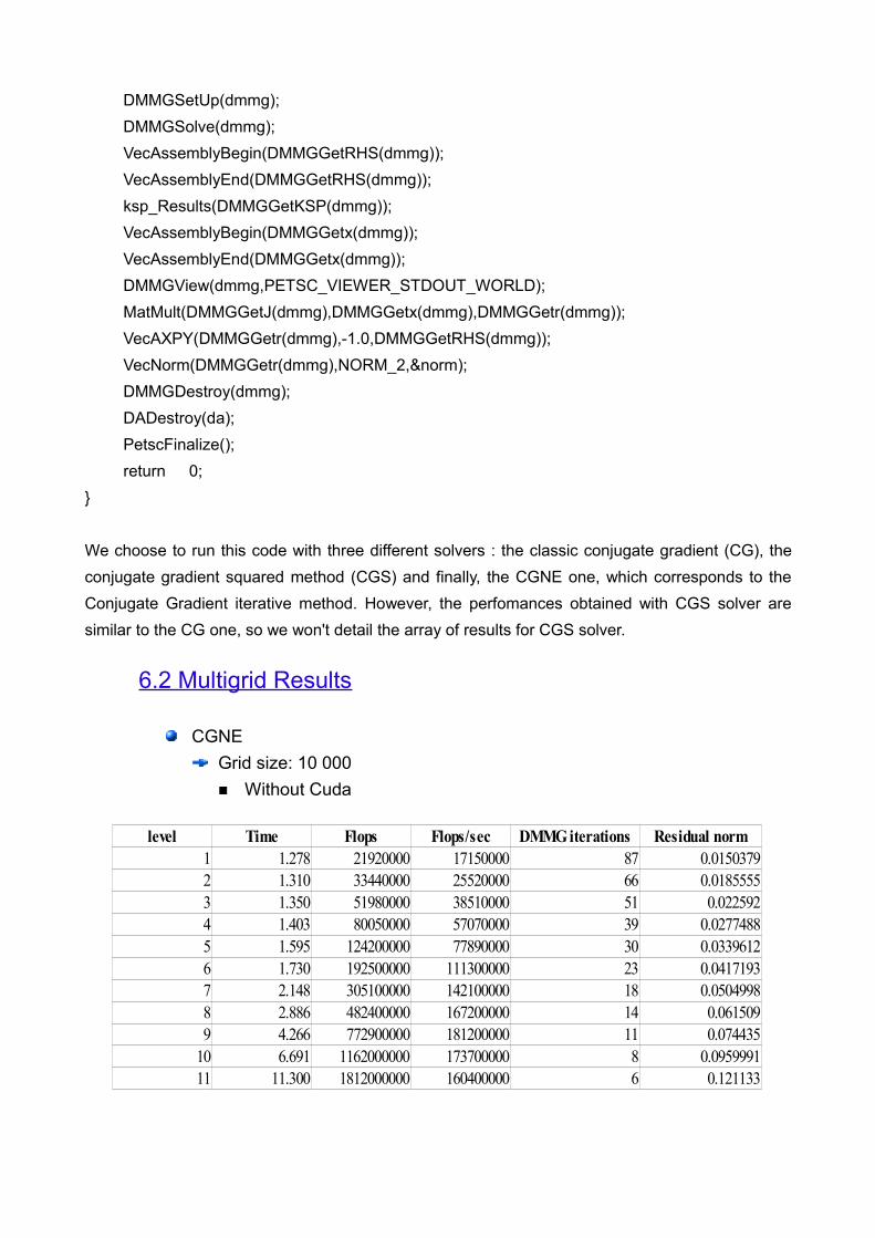
CGNEGrid size: 10 000■ Without Cuda
level Time Flops Flops/sec DMMG iterations Residual norm1 1.278 21920000 17150000 87 0.01503792 1.310 33440000 25520000 66 0.01855553 1.350 51980000 38510000 51 0.0225924 1.403 80050000 57070000 39 0.02774885 1.595 124200000 77890000 30 0.03396126 1.730 192500000 111300000 23 0.04171937 2.148 305100000 142100000 18 0.05049988 2.886 482400000 167200000 14 0.0615099 4.266 772900000 181200000 11 0.074435
10 6.691 1162000000 173700000 8 0.095999111 11.300 1812000000 160400000 6 0.121133
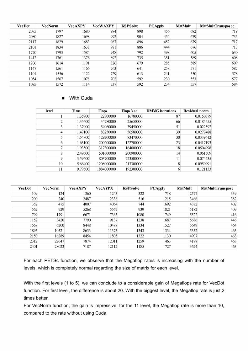
■ With Cuda
For each PETSc function, we observe that the Megaflop rates is increasing with the number of levels, which is completely normal regarding the size of matrix for each level.
With the first levels (1 to 5), we can conclude to a considerable gain of Megaflops rate for VecDot function. For first level, the difference is about 20. With the biggest level, the Megaflop rate is just 2 times better.For VecNorm function, the gain is impressive: for the 11 level, the Megaflop rate is more than 10, compared to the rate without using Cuda.
VecDot VecNorm VecAXPY VecWAXPY KSPSolve PCApply MatMult MatMultTransposee2085 1797 1680 984 898 456 682 7192080 1827 1698 992 904 454 679 7352117 1829 1683 987 896 452 679 7172101 1834 1638 981 886 444 676 7131720 1793 1584 948 792 398 605 6301412 1761 1376 892 735 351 589 6081206 1614 1191 826 679 285 589 6091147 1561 1166 763 641 258 571 5871101 1556 1122 729 613 241 550 5781054 1567 1078 702 592 230 553 5771095 1572 1114 737 592 234 557 584
level Time Flops Flops/sec DMMG iterations Residual norm1 1.35900 22800000 16780000 87 0.01503792 1.35600 34780000 25650000 66 0.01855553 1.37000 54060000 39450000 51 0.0225924 1.47100 83250000 56580000 39 0.02774885 1.54800 129200000 83470000 30 0.03396126 1.63100 200200000 122700000 23 0.04171937 1.93500 317300000 164000000 18 0.05049988 2.49600 501600000 200900000 14 0.0615099 3.59600 803700000 223500000 11 0.074435
10 5.66400 1208000000 213300000 8 0.095999111 9.79500 1884000000 192300000 6 0.121133
VecDot VecNorm VecAXPY VecAYPX KSPSolve PCApply MatMult MatMultTranspose109 124 1360 1243 322 718 2577 339200 240 2487 2338 516 1215 3466 382352 475 4007 4054 744 1692 4382 402562 929 5268 5567 939 1821 5182 409799 1791 6671 7363 1080 1749 5522 416
1152 3420 7790 9137 1238 1687 5686 4461568 6200 8448 10488 1334 1527 5649 4641895 10521 8633 11373 1343 1334 5352 4632150 16289 8454 11805 1322 1130 4907 4632312 22647 7874 12011 1259 463 4188 4632401 28023 7187 12112 1185 727 3624 463
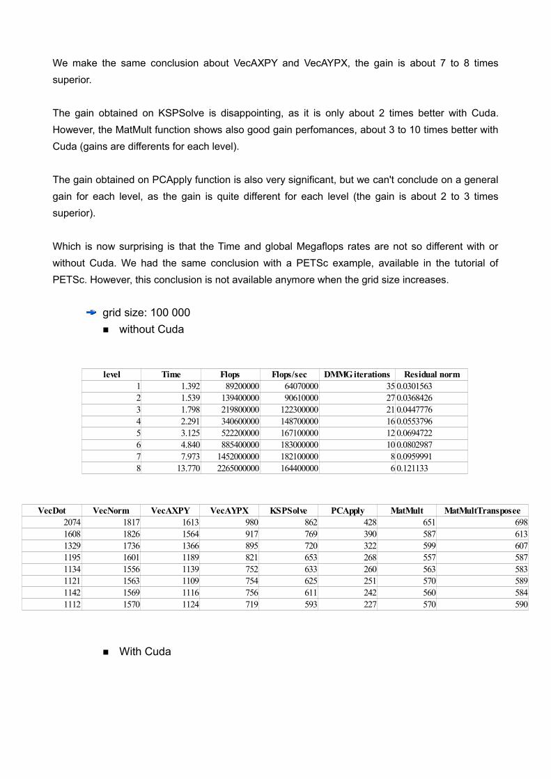
We make the same conclusion about VecAXPY and VecAYPX, the gain is about 7 to 8 times superior.
The gain obtained on KSPSolve is disappointing, as it is only about 2 times better with Cuda. However, the MatMult function shows also good gain perfomances, about 3 to 10 times better with Cuda (gains are differents for each level).
The gain obtained on PCApply function is also very significant, but we can't conclude on a general gain for each level, as the gain is quite different for each level (the gain is about 2 to 3 times superior).
Which is now surprising is that the Time and global Megaflops rates are not so different with or without Cuda. We had the same conclusion with a PETSc example, available in the tutorial of PETSc. However, this conclusion is not available anymore when the grid size increases.
grid size: 100 000■ without Cuda
■ With Cuda
level Time Flops Flops/sec DMMG iterations Residual norm1 1.392 89200000 64070000 35 0.03015632 1.539 139400000 90610000 27 0.03684263 1.798 219800000 122300000 21 0.04477764 2.291 340600000 148700000 16 0.05537965 3.125 522200000 167100000 12 0.06947226 4.840 885400000 183000000 10 0.08029877 7.973 1452000000 182100000 8 0.09599918 13.770 2265000000 164400000 6 0.121133
VecDot VecNorm VecAXPY VecAYPX KSPSolve PCApply MatMult MatMultTransposee2074 1817 1613 980 862 428 651 6981608 1826 1564 917 769 390 587 6131329 1736 1366 895 720 322 599 6071195 1601 1189 821 653 268 557 5871134 1556 1139 752 633 260 563 5831121 1563 1109 754 625 251 570 5891142 1569 1116 756 611 242 560 5841112 1570 1124 719 593 227 570 590
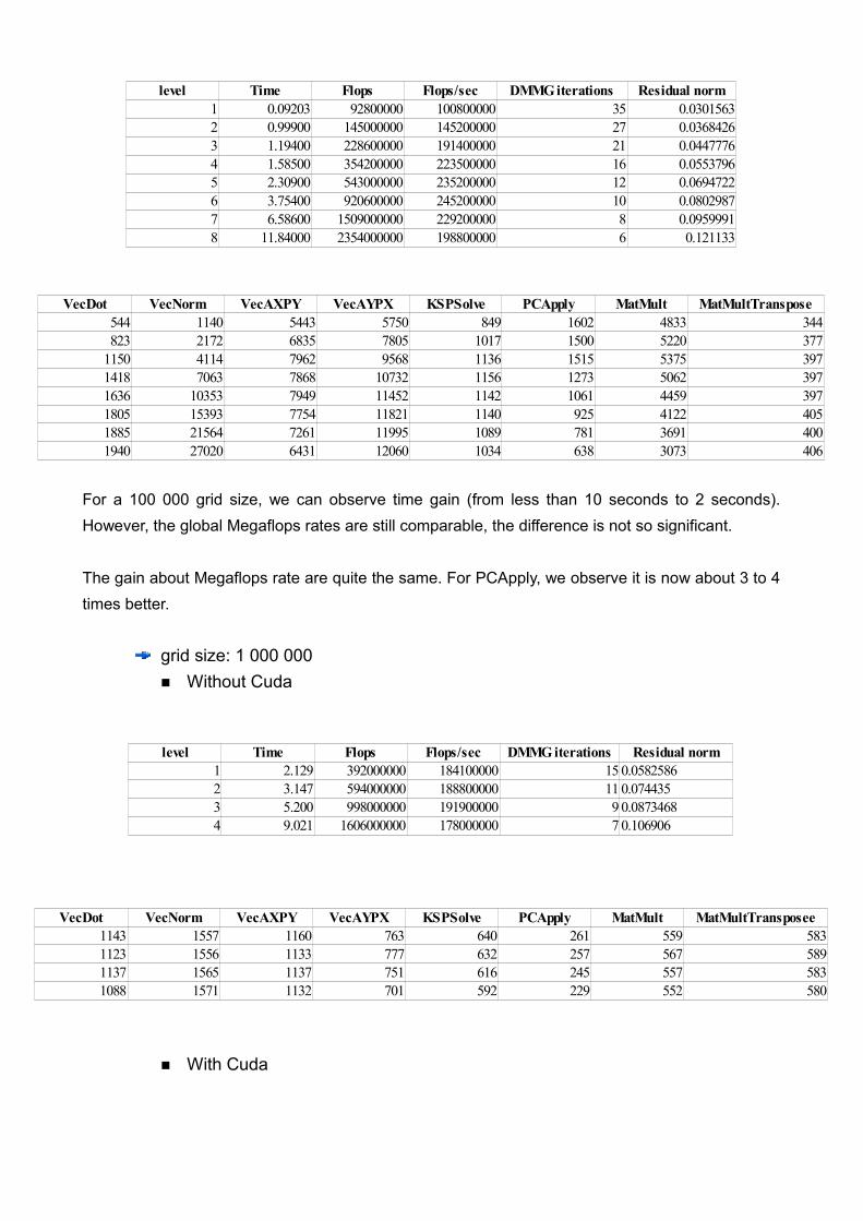
For a 100 000 grid size, we can observe time gain (from less than 10 seconds to 2 seconds). However, the global Megaflops rates are still comparable, the difference is not so significant.
The gain about Megaflops rate are quite the same. For PCApply, we observe it is now about 3 to 4 times better.
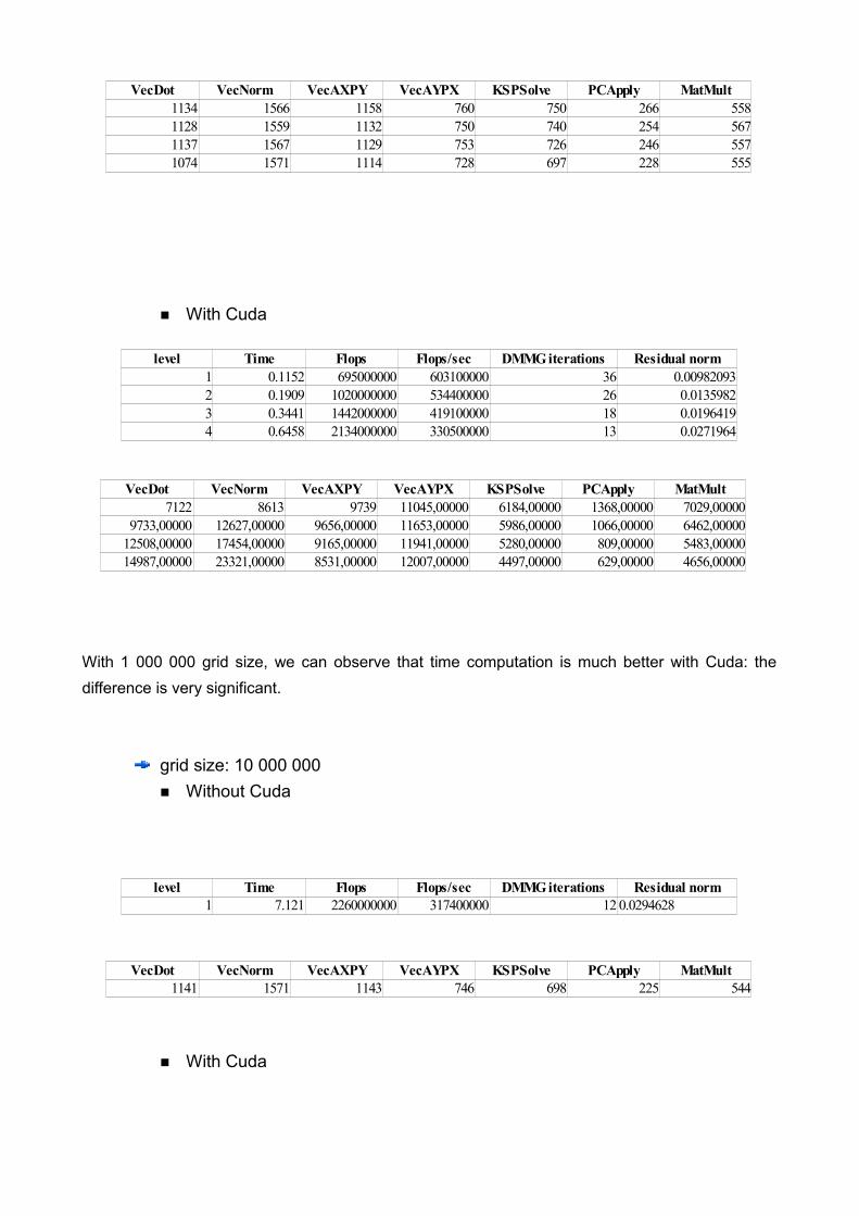
grid size: 1 000 000■ Without Cuda
■ With Cuda
level Time Flops Flops/sec DMMG iterations Residual norm1 2.129 392000000 184100000 15 0.05825862 3.147 594000000 188800000 11 0.0744353 5.200 998000000 191900000 9 0.08734684 9.021 1606000000 178000000 7 0.106906
VecDot VecNorm VecAXPY VecAYPX KSPSolve PCApply MatMult MatMultTransposee1143 1557 1160 763 640 261 559 5831123 1556 1133 777 632 257 567 5891137 1565 1137 751 616 245 557 5831088 1571 1132 701 592 229 552 580
level Time Flops Flops/sec DMMG iterations Residual norm1 0.09203 92800000 100800000 35 0.03015632 0.99900 145000000 145200000 27 0.03684263 1.19400 228600000 191400000 21 0.04477764 1.58500 354200000 223500000 16 0.05537965 2.30900 543000000 235200000 12 0.06947226 3.75400 920600000 245200000 10 0.08029877 6.58600 1509000000 229200000 8 0.09599918 11.84000 2354000000 198800000 6 0.121133
VecDot VecNorm VecAXPY VecAYPX KSPSolve PCApply MatMult MatMultTranspose544 1140 5443 5750 849 1602 4833 344823 2172 6835 7805 1017 1500 5220 377
1150 4114 7962 9568 1136 1515 5375 3971418 7063 7868 10732 1156 1273 5062 3971636 10353 7949 11452 1142 1061 4459 3971805 15393 7754 11821 1140 925 4122 4051885 21564 7261 11995 1089 781 3691 4001940 27020 6431 12060 1034 638 3073 406
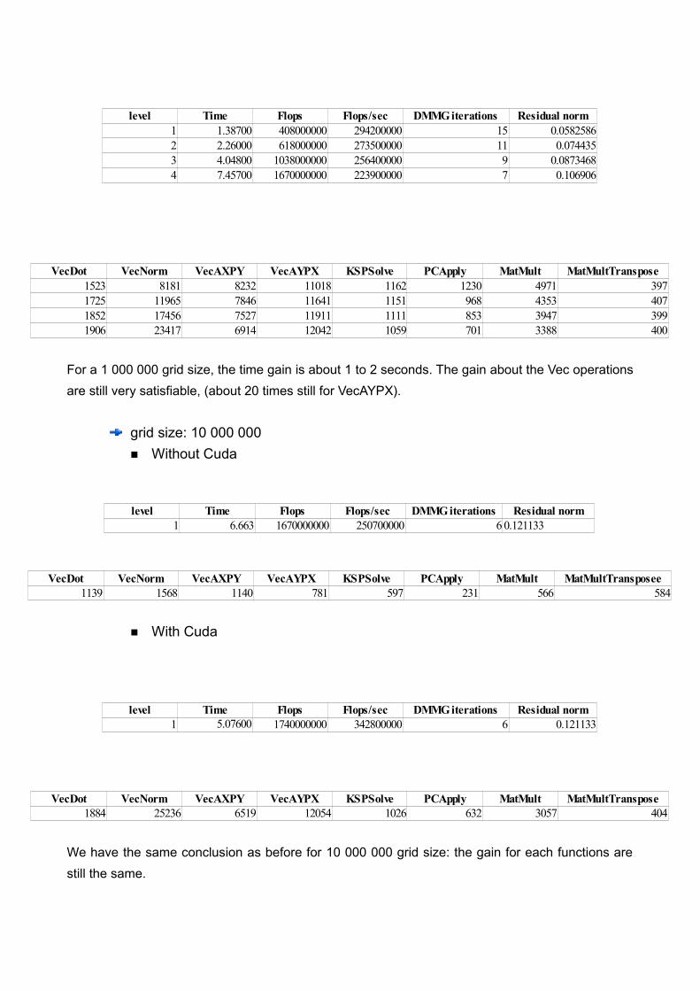
For a 1 000 000 grid size, the time gain is about 1 to 2 seconds. The gain about the Vec operations are still very satisfiable, (about 20 times still for VecAYPX).
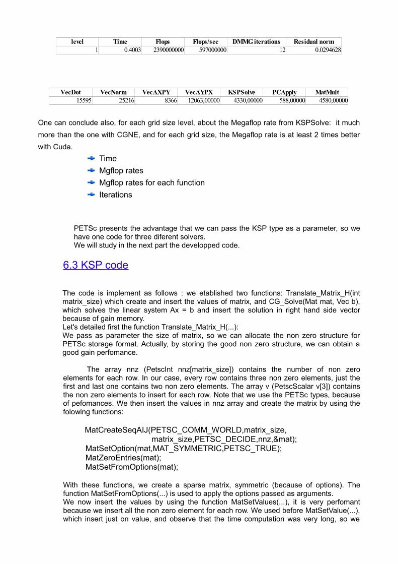
grid size: 10 000 000■ Without Cuda
■ With Cuda
We have the same conclusion as before for 10 000 000 grid size: the gain for each functions are still the same.
level Time Flops Flops/sec DMMG iterations Residual norm1 6.663 1670000000 250700000 6 0.121133
VecDot VecNorm VecAXPY VecAYPX KSPSolve PCApply MatMult MatMultTransposee1139 1568 1140 781 597 231 566 584
level Time Flops Flops/sec DMMG iterations Residual norm1 1.38700 408000000 294200000 15 0.05825862 2.26000 618000000 273500000 11 0.0744353 4.04800 1038000000 256400000 9 0.08734684 7.45700 1670000000 223900000 7 0.106906
VecDot VecNorm VecAXPY VecAYPX KSPSolve PCApply MatMult MatMultTranspose1523 8181 8232 11018 1162 1230 4971 3971725 11965 7846 11641 1151 968 4353 4071852 17456 7527 11911 1111 853 3947 3991906 23417 6914 12042 1059 701 3388 400
level Time Flops Flops/sec DMMG iterations Residual norm1 1740000000 342800000 6 0.121133 5.07600
VecDot VecNorm VecAXPY VecAYPX KSPSolve PCApply MatMult MatMultTranspose1884 25236 6519 12054 1026 632 3057 404
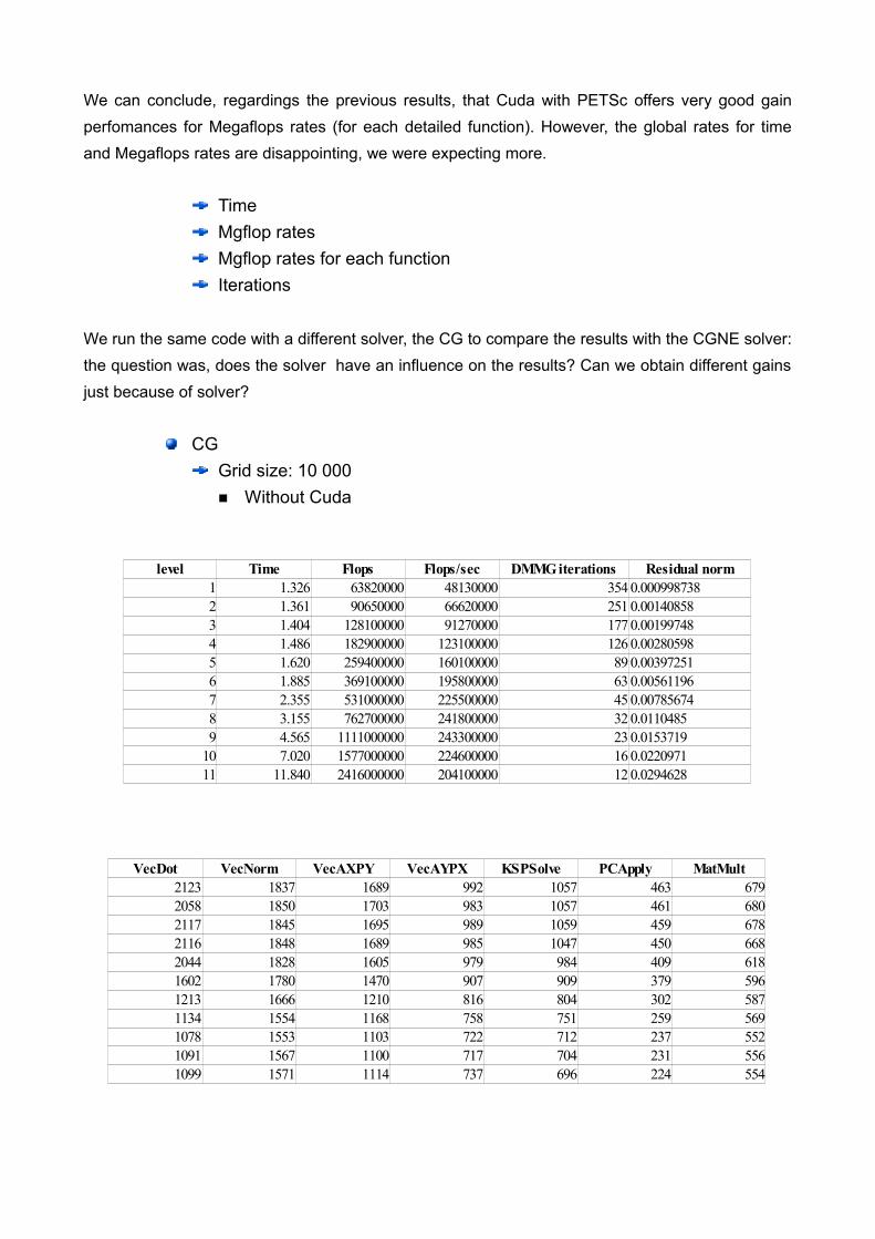
We can conclude, regardings the previous results, that Cuda with PETSc offers very good gain perfomances for Megaflops rates (for each detailed function). However, the global rates for time and Megaflops rates are disappointing, we were expecting more.
TimeMgflop ratesMgflop rates for each functionIterations
We run the same code with a different solver, the CG to compare the results with the CGNE solver: the question was, does the solver have an influence on the results? Can we obtain different gains just because of solver?
CGGrid size: 10 000■ Without Cuda
level Time Flops Flops/sec DMMG iterations Residual norm1 1.326 63820000 48130000 354 0.0009987382 1.361 90650000 66620000 251 0.001408583 1.404 128100000 91270000 177 0.001997484 1.486 182900000 123100000 126 0.002805985 1.620 259400000 160100000 89 0.003972516 1.885 369100000 195800000 63 0.005611967 2.355 531000000 225500000 45 0.007856748 3.155 762700000 241800000 32 0.01104859 4.565 1111000000 243300000 23 0.0153719
10 7.020 1577000000 224600000 16 0.022097111 11.840 2416000000 204100000 12 0.0294628
VecDot VecNorm VecAXPY VecAYPX KSPSolve PCApply MatMult2123 1837 1689 992 1057 463 6792058 1850 1703 983 1057 461 6802117 1845 1695 989 1059 459 6782116 1848 1689 985 1047 450 6682044 1828 1605 979 984 409 6181602 1780 1470 907 909 379 5961213 1666 1210 816 804 302 5871134 1554 1168 758 751 259 5691078 1553 1103 722 712 237 5521091 1567 1100 717 704 231 5561099 1571 1114 737 696 224 554
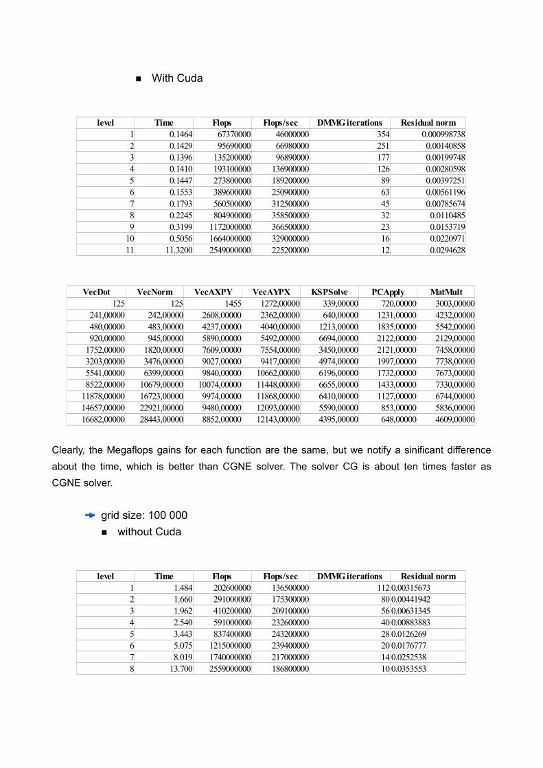
■ With Cuda
Clearly, the Megaflops gains for each function are the same, but we notify a sinificant difference about the time, which is better than CGNE solver. The solver CG is about ten times faster as CGNE solver.
grid size: 100 000■ without Cuda
level Time Flops Flops/sec DMMG iterations Residual norm1 1.484 202600000 136500000 112 0.003156732 1.660 291000000 175300000 80 0.004419423 1.962 410200000 209100000 56 0.006313454 2.540 591000000 232600000 40 0.008838835 3.443 837400000 243200000 28 0.01262696 5.075 1215000000 239400000 20 0.01767777 8.019 1740000000 217000000 14 0.02525388 13.700 2559000000 186800000 10 0.0353553
level Time Flops Flops/sec DMMG iterations Residual norm1 0.1464 67370000 46000000 354 0.0009987382 0.1429 95690000 66980000 251 0.001408583 0.1396 135200000 96890000 177 0.001997484 0.1410 193100000 136900000 126 0.002805985 0.1447 273800000 189200000 89 0.003972516 0.1553 389600000 250900000 63 0.005611967 0.1793 560500000 312500000 45 0.007856748 0.2245 804900000 358500000 32 0.01104859 0.3199 1172000000 366500000 23 0.0153719
10 0.5056 1664000000 329000000 16 0.022097111 11.3200 2549000000 225200000 12 0.0294628
VecDot VecNorm VecAXPY VecAYPX KSPSolve PCApply MatMult125 125 1455 1272,00000 339,00000 720,00000 3003,00000
241,00000 242,00000 2608,00000 2362,00000 640,00000 1231,00000 4232,00000480,00000 483,00000 4237,00000 4040,00000 1213,00000 1835,00000 5542,00000920,00000 945,00000 5890,00000 5492,00000 6694,00000 2122,00000 2129,00000
1752,00000 1820,00000 7609,00000 7554,00000 3450,00000 2121,00000 7458,000003203,00000 3476,00000 9027,00000 9417,00000 4974,00000 1997,00000 7738,000005541,00000 6399,00000 9840,00000 10662,00000 6196,00000 1732,00000 7673,000008522,00000 10679,00000 10074,00000 11448,00000 6655,00000 1433,00000 7330,00000
11878,00000 16723,00000 9974,00000 11868,00000 6410,00000 1127,00000 6744,0000014657,00000 22921,00000 9480,00000 12093,00000 5590,00000 853,00000 5836,0000016682,00000 28443,00000 8852,00000 12143,00000 4395,00000 648,00000 4609,00000
■ With Cuda
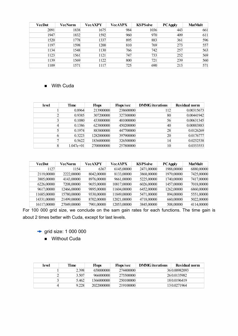
For 100 000 grid size, we conclude on the sam gain rates for each functions. The time gain is about 2 times better with Cuda, except for last levels.
grid size: 1 000 000■ Without Cuda
VecDot VecNorm VecAXPY VecAYPX KSPSolve PCApply MatMult2091 1838 1675 984 1036 443 6611947 1832 1592 960 970 409 6111520 1778 1337 895 883 361 5961197 1598 1200 810 769 273 5571134 1548 1130 766 742 257 5631123 1561 1121 747 733 252 5691139 1569 1122 800 721 239 5601109 1571 1117 725 690 213 571
level Time Flops Flops/sec DMMG iterations Residual norm1 2.398 658000000 274400000 36 0.009820932 3.507 966000000 275500000 26 0.01359823 5.462 1366000000 250100000 18 0.01964194 9.228 2022000000 219100000 13 0.0271964
level Time Flops Flops/sec DMMG iterations Residual norm1 0.8964 213900000 238600000 112 0.003156732 0.9385 307200000 327300000 80 0.004419423 0.1080 433000000 401000000 56 0.006313454 0.1386 623800000 450200000 40 0.008838835 0.1974 883800000 447700000 28 0.01262696 0.3223 1282000000 397900000 20 0.01767777 0.5622 1836000000 326500000 14 0.02525388 1.047e+01 2700000000 257800000 10 0.0353553
VecDot VecNorm VecAXPY VecAYPX KSPSolve PCApply MatMult1127 1154 6367 6145,00000 2471,00000 1988,00000 6880,00000
2119,00000 2222,00000 8042,00000 8133,00000 3868,00000 1979,00000 7425,000003805,00000 4143,00000 8976,00000 9661,00000 5225,00000 1740,00000 7417,000006226,00000 7208,00000 9655,00000 10817,00000 6026,00000 1457,00000 7018,000009617,00000 12466,00000 9895,00000 11604,00000 6452,00000 1262,00000 6860,00000
11685,00000 15780,00000 9330,00000 11849,00000 5471,00000 894,00000 5551,0000014331,00000 21499,00000 8702,00000 12021,00000 4718,00000 660,00000 5022,0000016117,00000 27049,00000 7901,00000 12053,00000 3845,00000 508,00000 4114,00000
■ With Cuda
With 1 000 000 grid size, we can observe that time computation is much better with Cuda: the difference is very significant.
grid size: 10 000 000■ Without Cuda
■ With Cuda
VecDot VecNorm VecAXPY VecAYPX KSPSolve PCApply MatMult1134 1566 1158 760 750 266 5581128 1559 1132 750 740 254 5671137 1567 1129 753 726 246 5571074 1571 1114 728 697 228 555
level Time Flops Flops/sec DMMG iterations Residual norm1 7.121 2260000000 317400000 12 0.0294628
VecDot VecNorm VecAXPY VecAYPX KSPSolve PCApply MatMult1141 1571 1143 746 698 225 544
level Time Flops Flops/sec DMMG iterations Residual norm1 0.1152 695000000 603100000 36 0.009820932 0.1909 1020000000 534400000 26 0.01359823 0.3441 1442000000 419100000 18 0.01964194 0.6458 2134000000 330500000 13 0.0271964
VecDot VecNorm VecAXPY VecAYPX KSPSolve PCApply MatMult7122 8613 9739 11045,00000 6184,00000 1368,00000 7029,00000
9733,00000 12627,00000 9656,00000 11653,00000 5986,00000 1066,00000 6462,0000012508,00000 17454,00000 9165,00000 11941,00000 5280,00000 809,00000 5483,0000014987,00000 23321,00000 8531,00000 12007,00000 4497,00000 629,00000 4656,00000
One can conclude also, for each grid size level, about the Megaflop rate from KSPSolve: it much more than the one with CGNE, and for each grid size, the Megaflop rate is at least 2 times better with Cuda.
TimeMgflop ratesMgflop rates for each functionIterations
PETSc presents the advantage that we can pass the KSP type as a parameter, so we have one code for three diferent solvers.We will study in the next part the developped code.
6.3 KSP code
The code is implement as follows : we etablished two functions: Translate_Matrix_H(int matrix_size) which create and insert the values of matrix, and CG_Solve(Mat mat, Vec b), which solves the linear system Ax = b and insert the solution in right hand side vector because of gain memory.Let's detailed first the function Translate_Matrix_H(...): We pass as parameter the size of matrix, so we can allocate the non zero structure for PETSc storage format. Actually, by storing the good non zero structure, we can obtain a good gain perfomance.
The array nnz (PetscInt nnz[matrix_size]) contains the number of non zero elements for each row. In our case, every row contains three non zero elements, just the first and last one contains two non zero elements. The array v (PetscScalar v[3]) contains the non zero elements to insert for each row. Note that we use the PETSc types, because of pefomances. We then insert the values in nnz array and create the matrix by using the folowing functions:
MatCreateSeqAIJ(PETSC_COMM_WORLD,matrix_size, matrix_size,PETSC_DECIDE,nnz,&mat);
MatSetOption(mat,MAT_SYMMETRIC,PETSC_TRUE);MatZeroEntries(mat);MatSetFromOptions(mat);
With these functions, we create a sparse matrix, symmetric (because of options). The function MatSetFromOptions(...) is used to apply the options passed as arguments.We now insert the values by using the function MatSetValues(...), it is very perfomant because we insert all the non zero element for each row. We used before MatSetValue(...), which insert just on value, and observe that the time computation was very long, so we
level Time Flops Flops/sec DMMG iterations Residual norm1 0.4003 2390000000 597000000 12 0.0294628
VecDot VecNorm VecAXPY VecAYPX KSPSolve PCApply MatMult15595 25216 8366 12063,00000 4330,00000 588,00000 4580,00000
optimized the code by insert all the values for each row.
Mat Translate_Matrix_H(int matrix_size){
Mat mat; PetscInt idxm[1],idxn[3];PetscScalar v[3];PetscInt nnz[matrix_size]; PetscFunctionBegin;
MatCreate(PETSC_COMM_WORLD,&mat);nnz[0] = 2;nnz[matrix_size-1] = 2;for(i=1;i<matrix_size-1;i++) { nnz[i] = 3; }
MatCreateSeqAIJ(PETSC_COMM_WORLD,matrix_size, matrix_size,PETSC_DECIDE,nnz,&mat);
MatSetOption(mat,MAT_SYMMETRIC,PETSC_TRUE);MatZeroEntries(mat);MatSetFromOptions(mat);
idxm[0] = 0; idxn[0] = 0; v[0] = 1.0; idxn[1] = 1; v[1] = 0.5;MatSetValues(mat,1,idxm,2,idxn,v,INSERT_VALUES);
for(i=1;i<matrix_size-1;i++){idxm[0] = i;idxn[0] = i-1;v[0] = 0.5;idxn[1] = i;v[1] = 1.0;idxn[2] = i+1;v[2] = 0.5;MatSetValues(mat,1,idxm,3,idxn,v,INSERT_VALUES);
}idxm[0] = matrix_size-1;idxn[0] = matrix_size-2;v[0] = 0.5;idxn[1] = matrix_size-1;v[1] = 1.0;MatSetValues(mat,1,idxm,2,idxn,v,INSERT_VALUES);
MatAssemblyBegin(mat,MAT_FINAL_ASSEMBLY);MatAssemblyEnd(mat,MAT_FINAL_ASSEMBLY);return mat;
}
We will now detail the function which solves the linear system. The function CG_Solve(Mat mat, Vec b) has as parameter the matrix and righ hand side vector. We create the KSP context by using the function KSPCreate(...), then add a preconditioner with KSPGetPC(...). We can add also some options with KSPSetFromOptions(...): it considers the arguments passed when we run the code, such as the KSP type (CG, CGNE or CGS). The function KSPSolve(...) solve the linear system Ax = b. In our case, the final solution is stored in right hand side vector b.
KSP CG_Solve(Mat mat, Vec b)
{PC pc; KSP ksp; PetscReal normVector;KSPConvergedReason reason; int its;
PetscFunctionBegin;
KSPCreate(MPI_COMM_WORLD,&ksp);KSPSetOperators(ksp,mat,mat,DIFFERENT_NONZERO_PATTERN);KSPSetInitialGuessNonzero(ksp,PETSC_TRUE);KSPGetPC(ksp,&pc);PCSetType(pc,PCJACOBI);PCFactorSetShiftType(pc,MAT_SHIFT_POSITIVE_DEFINITE);KSPSetFromOptions(ksp);KSPSetNormType(ksp,KSP_NORM_PRECONDITIONED);KSPSetUp(ksp);
KSPSetTolerances(ksp,0.000010,0.000000,10000.000000,10000);KSPSolve(ksp,b,b);
KSPGetConvergedReason(ksp,&reason);if (reason==KSP_DIVERGED_INDEFINITE_PC) {
PetscPrintf(PETSC_COMM_WORLD,"\nDivergence because of indefinite preconditioner;\nRun the executable again but with '-pc_factor_shift_type POSITIVE_DEFINITE' option.\n",PETSC_VIEWER_STDOUT_WORLD);
} else{
if (reason<0) {PetscPrintf(PETSC_COMM_WORLD,"\nOther kind of
divergence: this should not happen: %f\n",reason,PETSC_VIEWER_STDOUT_WORLD);
} else {
KSPGetIterationNumber(ksp,&its);printf("\nConvergence in %d iterations.\n",(int)its);
}}
VecNorm(b,NORM_2,&normVector);return ksp;
}
int main(int argc,char **argv){
PetscInt n = 10;PetscMPIInt size;PetscErrorCode ierr;int matrix_size=524288;Mat A;Vec b;KSP ksp;
PetscInitialize(&argc,&argv,PETSC_NULL,help);
MPI_Comm_size(PETSC_COMM_WORLD,&size);
A=Translate_Matrix_H(matrix_size);
ierr = VecCreate(PETSC_COMM_WORLD,&b);CHKERRQ(ierr);ierr = VecSetSizes(b,PETSC_DECIDE,matrix_size);CHKERRQ(ierr);ierr = VecSetFromOptions(b);CHKERRQ(ierr);
ierr = VecSet(b,1.0);CHKERRQ(ierr);
ksp=CG_Solve(A,b);
KSPDestroy(ksp);MatDestroy(A);VecDestroy(b);
PetscFinalize();return 0;
}In our case, we decide to run this code with three different solvers (CG,CGNE and CGS).
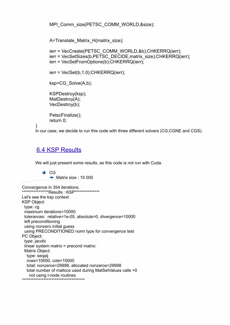
6.4 KSP Results
We will just present some results, as this code is not run with Cuda.
CGMatrix size : 10 000
Convergence in 354 iterations.****************Results : KSP***************Let's see the ksp contextKSP Object: type: cg maximum iterations=10000 tolerances: relative=1e-05, absolute=0, divergence=10000 left preconditioning using nonzero initial guess using PRECONDITIONED norm type for convergence testPC Object: type: jacobi linear system matrix = precond matrix: Matrix Object: type: seqaij rows=10000, cols=10000 total: nonzeros=29998, allocated nonzeros=29998 total number of mallocs used during MatSetValues calls =0 not using I-node routines**************************************
**************************************************************************************************************** WIDEN YOUR WINDOW TO 120 CHARACTERS. Use 'enscript -r -fCourier9' to print this document****************************************************************************************************************---------------------------------------------- PETSc Performance Summary:---------------------------------- Max Max/Min Avg Total Time (sec): 1.329e+00 1.00000 1.329e+00Objects: 1.300e+01 1.00000 1.300e+01Flops: 6.382e+07 1.00000 6.382e+07 6.382e+07Flops/sec: 4.803e+07 1.00000 4.803e+07 4.803e+07MPI Messages: 0.000e+00 0.00000 0.000e+00 0.000e+00MPI Message Lengths: 0.000e+00 0.00000 0.000e+00 0.000e+00MPI Reductions: 1.300e+01 1.00000
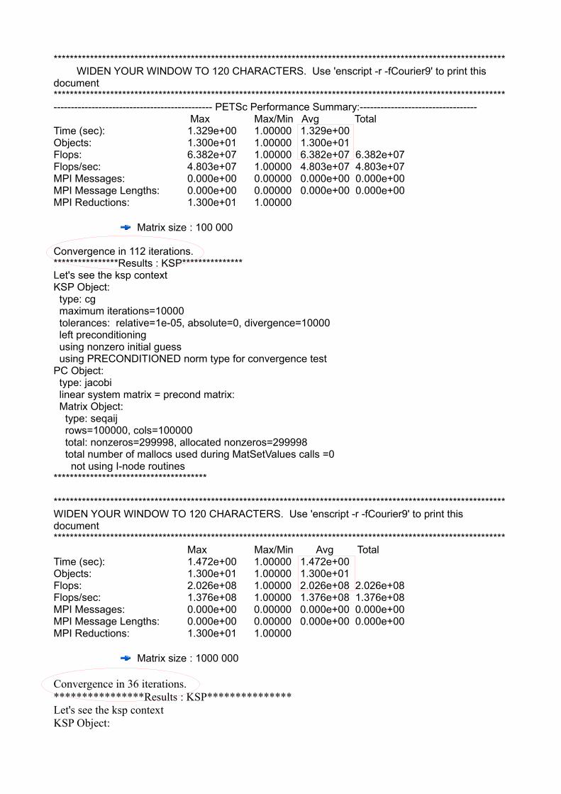
Matrix size : 100 000
Convergence in 112 iterations.****************Results : KSP***************Let's see the ksp contextKSP Object: type: cg maximum iterations=10000 tolerances: relative=1e-05, absolute=0, divergence=10000 left preconditioning using nonzero initial guess using PRECONDITIONED norm type for convergence testPC Object: type: jacobi linear system matrix = precond matrix: Matrix Object: type: seqaij rows=100000, cols=100000 total: nonzeros=299998, allocated nonzeros=299998 total number of mallocs used during MatSetValues calls =0 not using I-node routines**************************************
**************************************************************************************************************** WIDEN YOUR WINDOW TO 120 CHARACTERS. Use 'enscript -r -fCourier9' to print this document**************************************************************************************************************** Max Max/Min Avg Total Time (sec): 1.472e+00 1.00000 1.472e+00Objects: 1.300e+01 1.00000 1.300e+01Flops: 2.026e+08 1.00000 2.026e+08 2.026e+08Flops/sec: 1.376e+08 1.00000 1.376e+08 1.376e+08MPI Messages: 0.000e+00 0.00000 0.000e+00 0.000e+00MPI Message Lengths: 0.000e+00 0.00000 0.000e+00 0.000e+00MPI Reductions: 1.300e+01 1.00000
Matrix size : 1000 000
Convergence in 36 iterations.****************Results : KSP***************Let's see the ksp contextKSP Object:
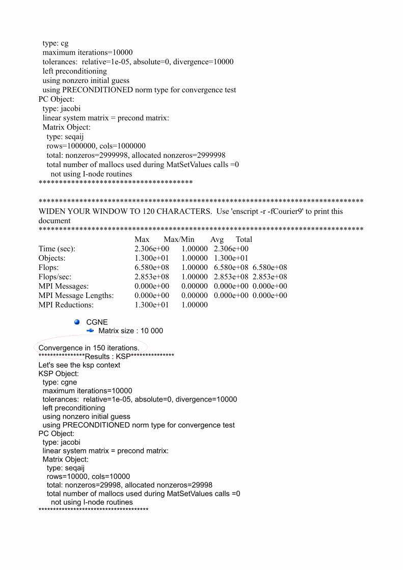
type: cg maximum iterations=10000 tolerances: relative=1e-05, absolute=0, divergence=10000 left preconditioning using nonzero initial guess using PRECONDITIONED norm type for convergence testPC Object: type: jacobi linear system matrix = precond matrix: Matrix Object: type: seqaij rows=1000000, cols=1000000 total: nonzeros=2999998, allocated nonzeros=2999998 total number of mallocs used during MatSetValues calls =0 not using I-node routines**************************************
********************************************************************************WIDEN YOUR WINDOW TO 120 CHARACTERS. Use 'enscript -r -fCourier9' to print this document ******************************************************************************** Max Max/Min Avg Total Time (sec): 2.306e+00 1.00000 2.306e+00Objects: 1.300e+01 1.00000 1.300e+01Flops: 6.580e+08 1.00000 6.580e+08 6.580e+08Flops/sec: 2.853e+08 1.00000 2.853e+08 2.853e+08MPI Messages: 0.000e+00 0.00000 0.000e+00 0.000e+00MPI Message Lengths: 0.000e+00 0.00000 0.000e+00 0.000e+00MPI Reductions: 1.300e+01 1.00000
CGNEMatrix size : 10 000
Convergence in 150 iterations.****************Results : KSP***************Let's see the ksp contextKSP Object: type: cgne maximum iterations=10000 tolerances: relative=1e-05, absolute=0, divergence=10000 left preconditioning using nonzero initial guess using PRECONDITIONED norm type for convergence testPC Object: type: jacobi linear system matrix = precond matrix: Matrix Object: type: seqaij rows=10000, cols=10000 total: nonzeros=29998, allocated nonzeros=29998 total number of mallocs used during MatSetValues calls =0 not using I-node routines**************************************
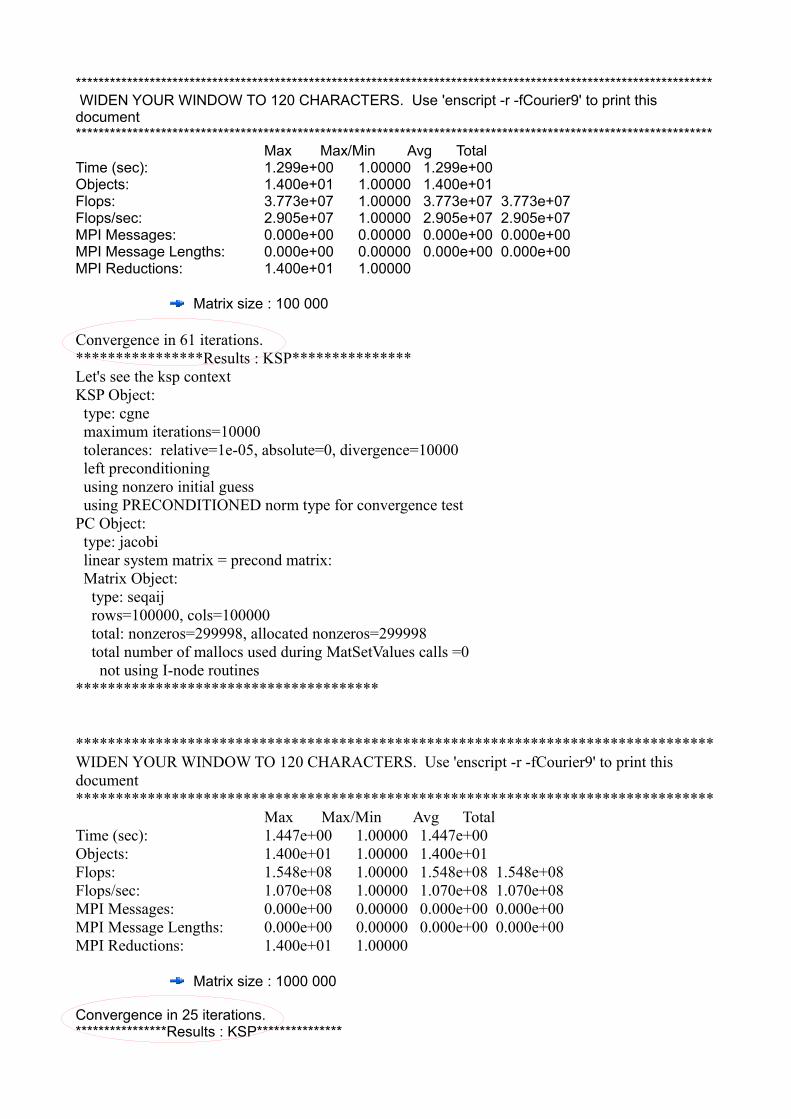
**************************************************************************************************************** WIDEN YOUR WINDOW TO 120 CHARACTERS. Use 'enscript -r -fCourier9' to print this document **************************************************************************************************************** Max Max/Min Avg Total Time (sec): 1.299e+00 1.00000 1.299e+00Objects: 1.400e+01 1.00000 1.400e+01Flops: 3.773e+07 1.00000 3.773e+07 3.773e+07Flops/sec: 2.905e+07 1.00000 2.905e+07 2.905e+07MPI Messages: 0.000e+00 0.00000 0.000e+00 0.000e+00MPI Message Lengths: 0.000e+00 0.00000 0.000e+00 0.000e+00MPI Reductions: 1.400e+01 1.00000
Matrix size : 100 000
Convergence in 61 iterations.****************Results : KSP***************Let's see the ksp contextKSP Object: type: cgne maximum iterations=10000 tolerances: relative=1e-05, absolute=0, divergence=10000 left preconditioning using nonzero initial guess using PRECONDITIONED norm type for convergence testPC Object: type: jacobi linear system matrix = precond matrix: Matrix Object: type: seqaij rows=100000, cols=100000 total: nonzeros=299998, allocated nonzeros=299998 total number of mallocs used during MatSetValues calls =0 not using I-node routines**************************************
********************************************************************************WIDEN YOUR WINDOW TO 120 CHARACTERS. Use 'enscript -r -fCourier9' to print this document ******************************************************************************** Max Max/Min Avg Total Time (sec): 1.447e+00 1.00000 1.447e+00Objects: 1.400e+01 1.00000 1.400e+01Flops: 1.548e+08 1.00000 1.548e+08 1.548e+08Flops/sec: 1.070e+08 1.00000 1.070e+08 1.070e+08MPI Messages: 0.000e+00 0.00000 0.000e+00 0.000e+00MPI Message Lengths: 0.000e+00 0.00000 0.000e+00 0.000e+00MPI Reductions: 1.400e+01 1.00000
Matrix size : 1000 000
Convergence in 25 iterations.****************Results : KSP***************
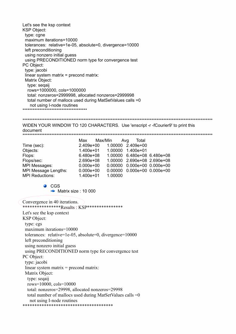
Let's see the ksp contextKSP Object: type: cgne maximum iterations=10000 tolerances: relative=1e-05, absolute=0, divergence=10000 left preconditioning using nonzero initial guess using PRECONDITIONED norm type for convergence testPC Object: type: jacobi linear system matrix = precond matrix: Matrix Object: type: seqaij rows=1000000, cols=1000000 total: nonzeros=2999998, allocated nonzeros=2999998 total number of mallocs used during MatSetValues calls =0 not using I-node routines**************************************
**************************************************************************************************************** WIDEN YOUR WINDOW TO 120 CHARACTERS. Use 'enscript -r -fCourier9' to print this document **************************************************************************************************************** Max Max/Min Avg Total Time (sec): 2.409e+00 1.00000 2.409e+00Objects: 1.400e+01 1.00000 1.400e+01Flops: 6.480e+08 1.00000 6.480e+08 6.480e+08Flops/sec: 2.690e+08 1.00000 2.690e+08 2.690e+08MPI Messages: 0.000e+00 0.00000 0.000e+00 0.000e+00MPI Message Lengths: 0.000e+00 0.00000 0.000e+00 0.000e+00MPI Reductions: 1.400e+01 1.00000
CGSMatrix size : 10 000
Convergence in 40 iterations.****************Results : KSP***************Let's see the ksp contextKSP Object: type: cgs maximum iterations=10000 tolerances: relative=1e-05, absolute=0, divergence=10000 left preconditioning using nonzero initial guess using PRECONDITIONED norm type for convergence testPC Object: type: jacobi linear system matrix = precond matrix: Matrix Object: type: seqaij rows=10000, cols=10000 total: nonzeros=29998, allocated nonzeros=29998 total number of mallocs used during MatSetValues calls =0 not using I-node routines**************************************
********************************************************************************WIDEN YOUR WINDOW TO 120 CHARACTERS. Use 'enscript -r -fCourier9' to print this document ********************************************************************************
Max Max/Min Avg Total Time (sec): 1.285e+00 1.00000 1.285e+00Objects: 1.700e+01 1.00000 1.700e+01Flops: 1.249e+07 1.00000 1.249e+07 1.249e+07Flops/sec: 9.720e+06 1.00000 9.720e+06 9.720e+06MPI Messages: 0.000e+00 0.00000 0.000e+00 0.000e+00MPI Message Lengths: 0.000e+00 0.00000 0.000e+00 0.000e+00MPI Reductions: 1.700e+01 1.00000
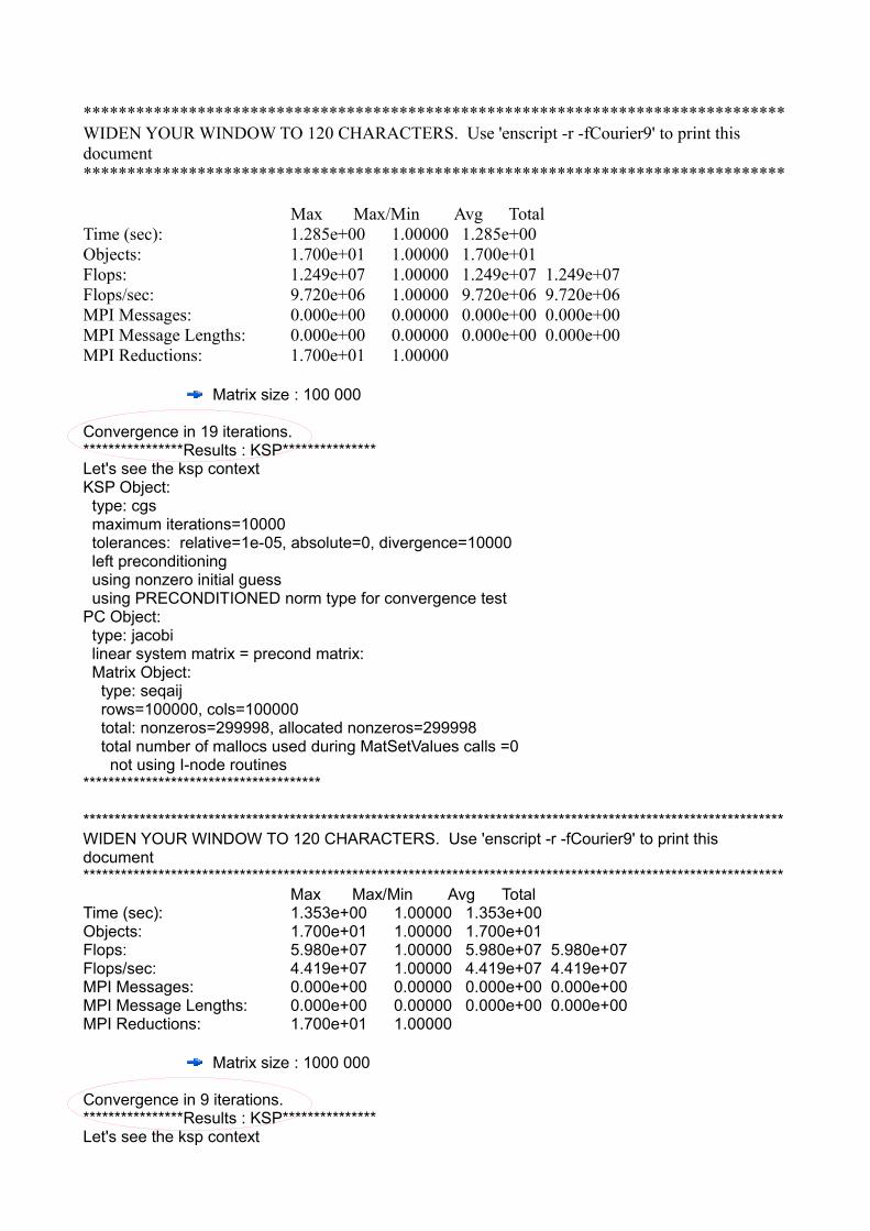
Matrix size : 100 000
Convergence in 19 iterations.****************Results : KSP***************Let's see the ksp contextKSP Object: type: cgs maximum iterations=10000 tolerances: relative=1e-05, absolute=0, divergence=10000 left preconditioning using nonzero initial guess using PRECONDITIONED norm type for convergence testPC Object: type: jacobi linear system matrix = precond matrix: Matrix Object: type: seqaij rows=100000, cols=100000 total: nonzeros=299998, allocated nonzeros=299998 total number of mallocs used during MatSetValues calls =0 not using I-node routines**************************************
****************************************************************************************************************WIDEN YOUR WINDOW TO 120 CHARACTERS. Use 'enscript -r -fCourier9' to print this document **************************************************************************************************************** Max Max/Min Avg Total Time (sec): 1.353e+00 1.00000 1.353e+00Objects: 1.700e+01 1.00000 1.700e+01Flops: 5.980e+07 1.00000 5.980e+07 5.980e+07Flops/sec: 4.419e+07 1.00000 4.419e+07 4.419e+07MPI Messages: 0.000e+00 0.00000 0.000e+00 0.000e+00MPI Message Lengths: 0.000e+00 0.00000 0.000e+00 0.000e+00MPI Reductions: 1.700e+01 1.00000
Matrix size : 1000 000
Convergence in 9 iterations.****************Results : KSP***************Let's see the ksp context
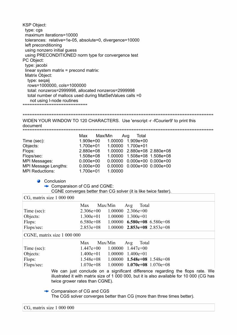
KSP Object: type: cgs maximum iterations=10000 tolerances: relative=1e-05, absolute=0, divergence=10000 left preconditioning using nonzero initial guess using PRECONDITIONED norm type for convergence testPC Object: type: jacobi linear system matrix = precond matrix: Matrix Object: type: seqaij rows=1000000, cols=1000000 total: nonzeros=2999998, allocated nonzeros=2999998 total number of mallocs used during MatSetValues calls =0 not using I-node routines**************************************
**************************************************************************************************************** WIDEN YOUR WINDOW TO 120 CHARACTERS. Use 'enscript -r -fCourier9' to print this document **************************************************************************************************************** Max Max/Min Avg Total Time (sec): 1.909e+00 1.00000 1.909e+00Objects: 1.700e+01 1.00000 1.700e+01Flops: 2.880e+08 1.00000 2.880e+08 2.880e+08Flops/sec: 1.508e+08 1.00000 1.508e+08 1.508e+08MPI Messages: 0.000e+00 0.00000 0.000e+00 0.000e+00MPI Message Lengths: 0.000e+00 0.00000 0.000e+00 0.000e+00MPI Reductions: 1.700e+01 1.00000
ConclusionComparaison of CG and CGNE:CGNE converges better than CG solver (it is like twice faster).
CG, matrix size 1 000 000 Max Max/Min Avg Total Time (sec): 2.306e+00 1.00000 2.306e+00Objects: 1.300e+01 1.00000 1.300e+01Flops: 6.580e+08 1.00000 6.580e+08 6.580e+08Flops/sec: 2.853e+08 1.00000 2.853e+08 2.853e+08CGNE, matrix size 1 000 000 Max Max/Min Avg Total Time (sec): 1.447e+00 1.00000 1.447e+00Objects: 1.400e+01 1.00000 1.400e+01Flops: 1.548e+08 1.00000 1.548e+08 1.548e+08Flops/sec: 1.070e+08 1.00000 1.070e+08 1.070e+08
We can just conclude on a significant difference regarding the flops rate. We illustrated it with matrix size of 1 000 000, but it is also available for 10 000 (CG has twice grower rates than CGNE).
Comparaison of CG and CGSThe CGS solver converges better than CG (more than three times better).
CG, matrix size 1 000 000
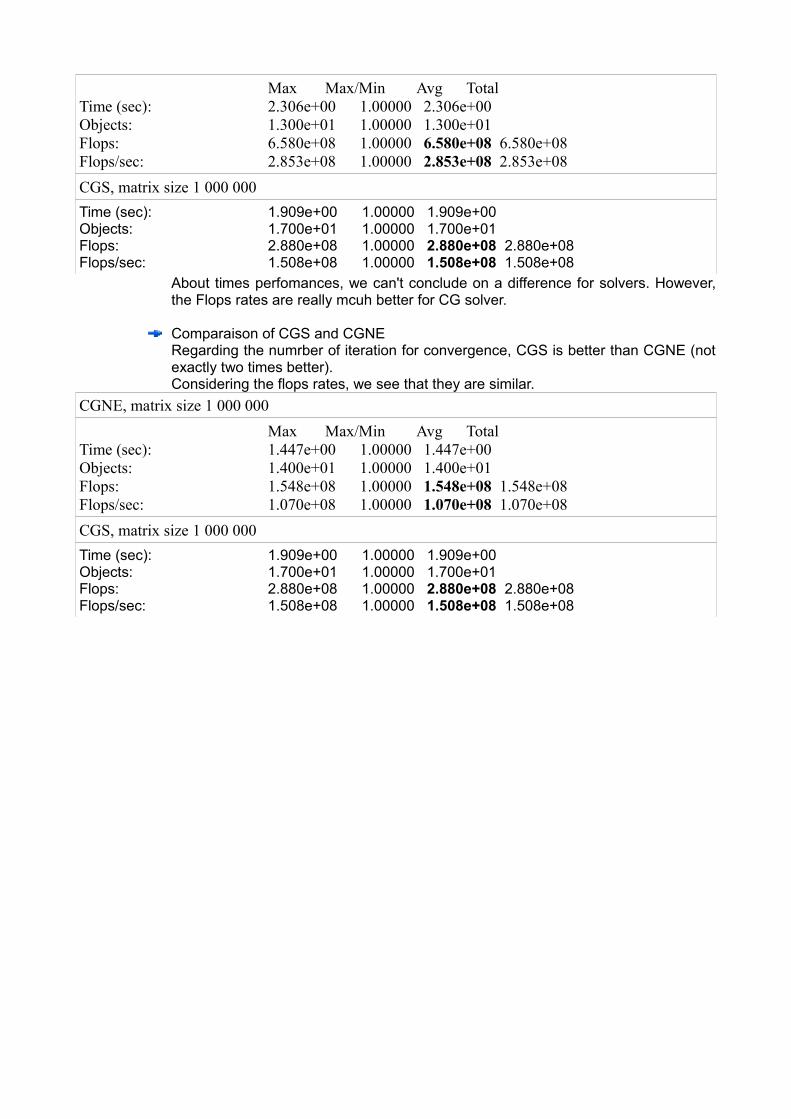
Max Max/Min Avg Total Time (sec): 2.306e+00 1.00000 2.306e+00Objects: 1.300e+01 1.00000 1.300e+01Flops: 6.580e+08 1.00000 6.580e+08 6.580e+08Flops/sec: 2.853e+08 1.00000 2.853e+08 2.853e+08CGS, matrix size 1 000 000 Time (sec): 1.909e+00 1.00000 1.909e+00Objects: 1.700e+01 1.00000 1.700e+01Flops: 2.880e+08 1.00000 2.880e+08 2.880e+08Flops/sec: 1.508e+08 1.00000 1.508e+08 1.508e+08
About times perfomances, we can't conclude on a difference for solvers. However, the Flops rates are really mcuh better for CG solver.
Comparaison of CGS and CGNERegarding the numrber of iteration for convergence, CGS is better than CGNE (not exactly two times better).Considering the flops rates, we see that they are similar.
CGNE, matrix size 1 000 000 Max Max/Min Avg Total Time (sec): 1.447e+00 1.00000 1.447e+00Objects: 1.400e+01 1.00000 1.400e+01Flops: 1.548e+08 1.00000 1.548e+08 1.548e+08Flops/sec: 1.070e+08 1.00000 1.070e+08 1.070e+08CGS, matrix size 1 000 000 Time (sec): 1.909e+00 1.00000 1.909e+00Objects: 1.700e+01 1.00000 1.700e+01Flops: 2.880e+08 1.00000 2.880e+08 2.880e+08Flops/sec: 1.508e+08 1.00000 1.508e+08 1.508e+08
VII GPU used in neutronic domainThe aim of this project was to implement the Conjugate Gradient method on GPU, by using CUDA, but also Cublas. We studied before the perfomances of Cublas and CUDA on scalar product examples, and it appears that CUDA offers a good gain perfomance, but still less than Cublas. In this context, we decide to apply it in neutronic domain, as the time and Megaflops rates gain must be more and more bigger.In what follows, we will study the architecture of codes, and explain our implementation choices.Then, we will briefly explain the CUDA's code, and Cublas one. We will finally present the obtained results.
7.1 Introduction
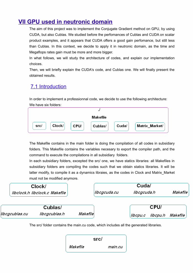
In order to implement a professionnal code, we decide to use the following architecture: We have six folders:
The Makefile contains in the main folder is doing the compilation of all codes in subsidiary folders. This Makefile contains the variables necesary to export the compiler path, and the command to execute the compilations in all subsidiary folders.In each subsidiary folders, excepted the src/ one, we have statics libraries: all Makefiles in subsidiary folders are compiling the codes such that we obtain statics libraries. It will be latter modify, to compile it as a dynamics libraies, as the codes in Clock and Matrix_Market must not be modified anymore.
The src/ folder contains the main.cu code, which includes all the generated libraries.
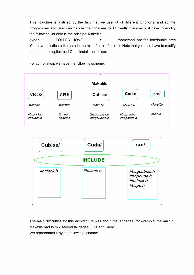
This structure is justified by the fact that we use lot of different functions, and so the programmer and user can handle the code easilly. Currently, the user just have to modify the following variable in the principal Makefile: export FOLDER_HOME = /home/phd_hpc/fboillod/double_precYou have to indicate the path to the main folder of project. Note that you also have to modify th epath to compiler, and Cuda installation folder.
For compilation, we have the following scheme:
The main difficulties for this architecture was about the langages: for example, the main.cu Makefile had to mix several langages (C++ and Cuda).We represented it by the following scheme:
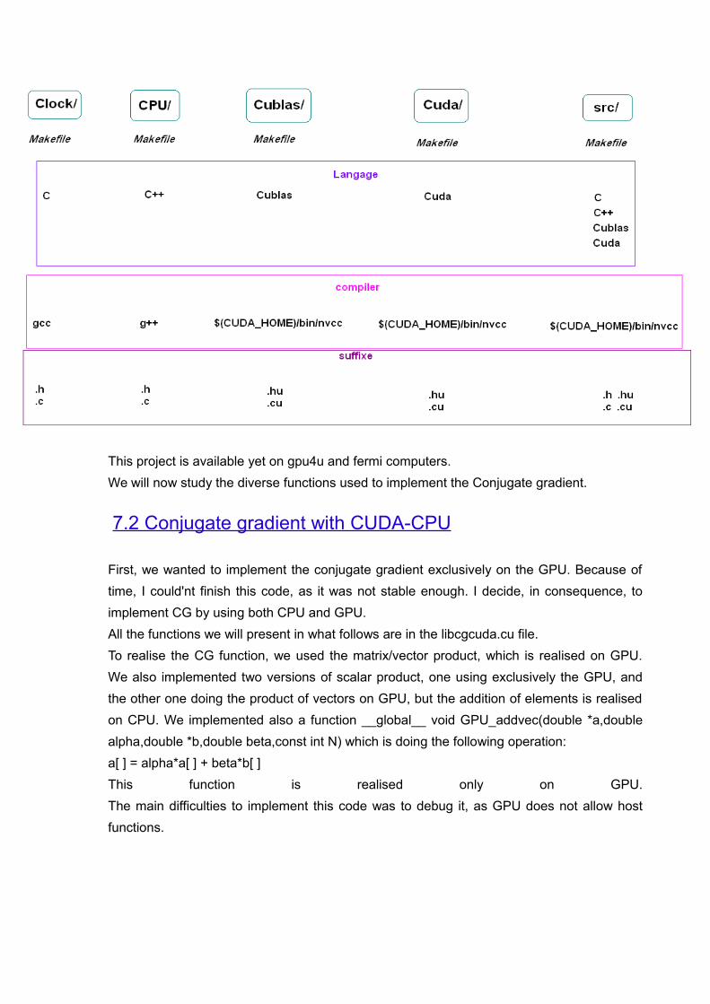
This project is available yet on gpu4u and fermi computers.We will now study the diverse functions used to implement the Conjugate gradient.
7.2 Conjugate gradient with CUDA-CPU
First, we wanted to implement the conjugate gradient exclusively on the GPU. Because of time, I could'nt finish this code, as it was not stable enough. I decide, in consequence, to implement CG by using both CPU and GPU.All the functions we will present in what follows are in the libcgcuda.cu file.To realise the CG function, we used the matrix/vector product, which is realised on GPU. We also implemented two versions of scalar product, one using exclusively the GPU, and the other one doing the product of vectors on GPU, but the addition of elements is realised on CPU. We implemented also a function __global__ void GPU_addvec(double *a,double alpha,double *b,double beta,const int N) which is doing the following operation: a[ ] = alpha*a[ ] + beta*b[ ]This function is realised only on GPU.The main difficulties to implement this code was to debug it, as GPU does not allow host functions.
7.3 Conjugate gradient with Cublas
The Cublas version of Conjugate Gradient was more easier to implement, as we can debug it quicklier. Actually, it exists a function CublasGetVector(...) so we can obtain the copy of device vector on a host vector.
Besides, the Cublas functions are easy to handle. We use, to implement the Conjugate Gradient function the following Cublas functions:
cublasDcopy ( n, b_d, 1, h_d, 1);This function copy the vector b in h one.
cublasDgemv ('N', n, n, 1.0, A_d, n, h_d, 1, 0.0, temp_Ah, 1);This function realises the following function:temp_Ah = 1.0 * A*h + 0.0 * temp_Ah
cublasDscal (n, v, h_d, 1);This function is doing the scalar product of v and h.
cublasDaxpy (n, -1.0, g_d, 1, h_d, 1);This function realises the following operation:h = -1.0 * g
norm_cub = cublasDdot (n, x_d, 1, x_d, 1);This function calculates the norm of x vector.
The function we created is the following: void GPU_CG_CUBLAS (double *A_d, double *x_d, double *b_d, double *vecnul_d, int n, int LOOP,double epsilon, const int nBytes,int *its_cublas,dim3 dimGrid)
A is the matrix (on device), b the right hand side, and x the initial solution. Vecnul is a vector on device which contains only nul values, as the cublas vectors are not initialized when you create them. N is the size of vector (and matrix, we used a squared one). LOOP is just the maximum iterations we allow, and epsilon, the error we fixed to stop the iteration (0.0001). its_cublas is the number of iterations at convergence, and other variables are used for memory allocation.
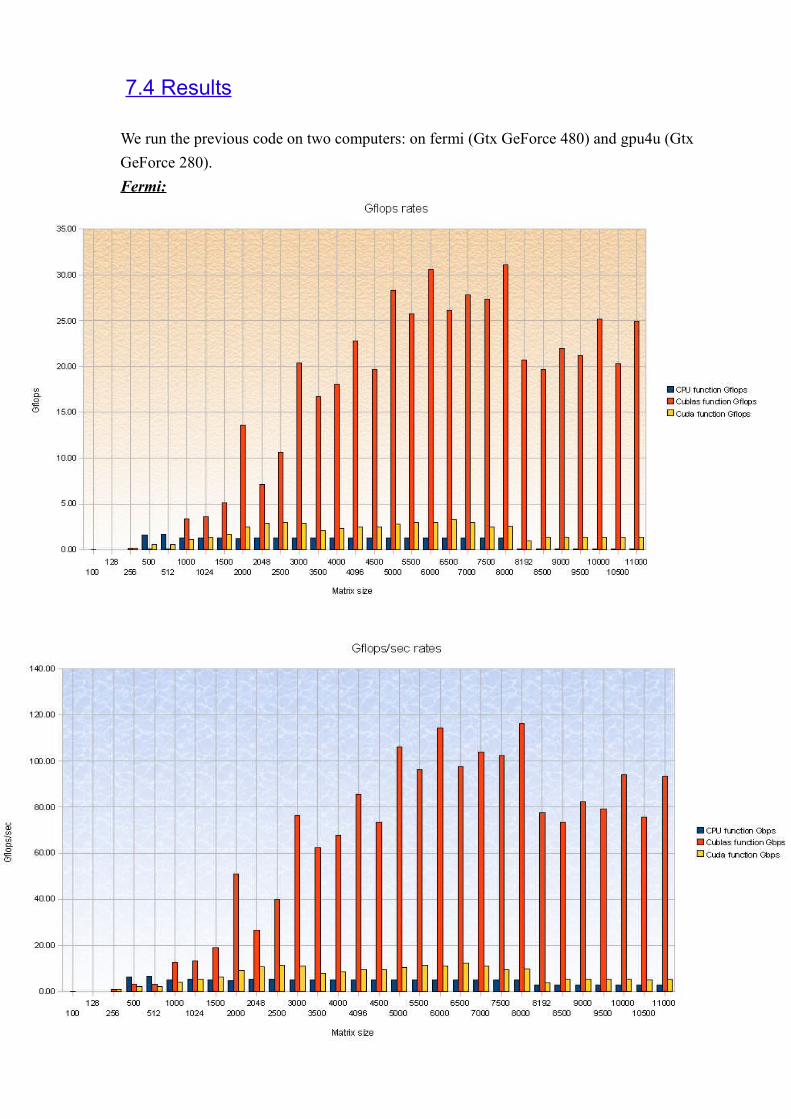
7.4 Results
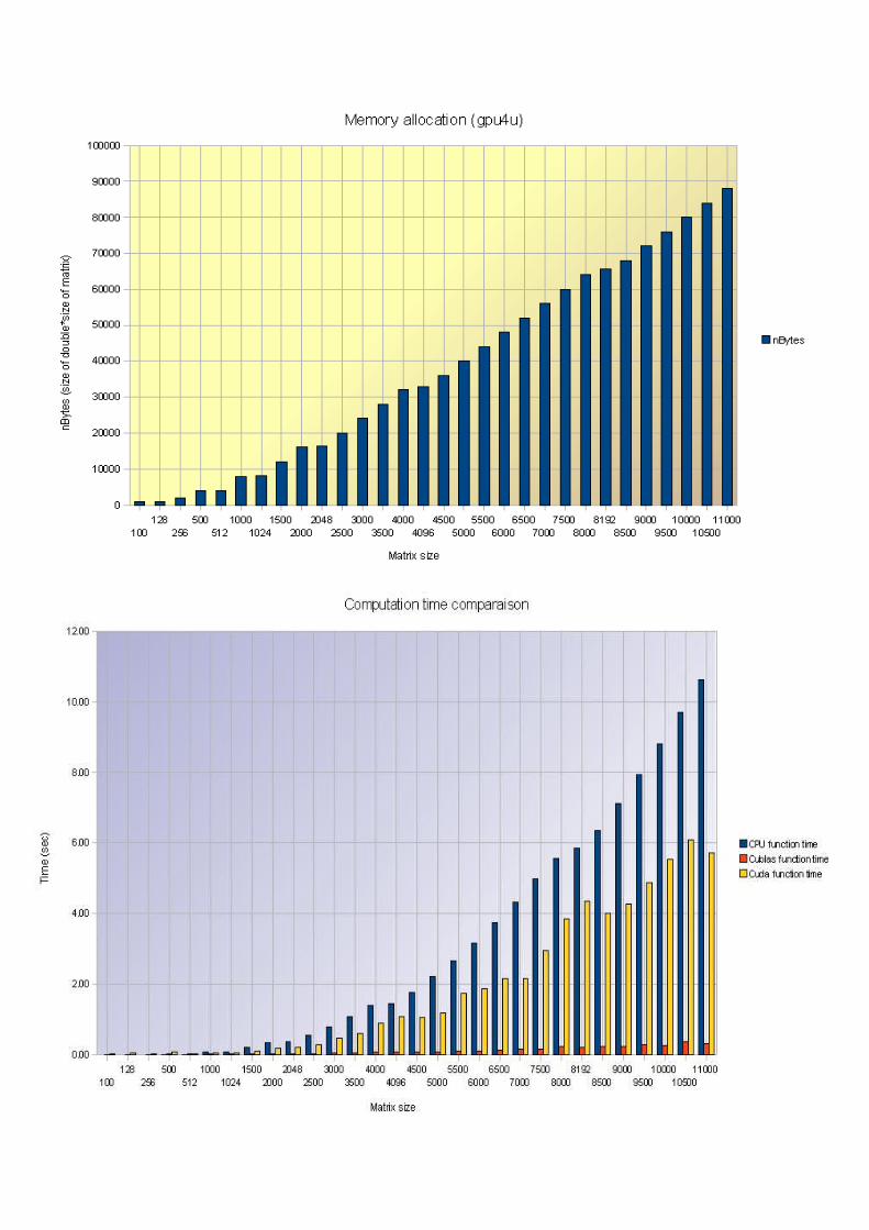
We run the previous code on two computers: on fermi (Gtx GeForce 480) and gpu4u (Gtx GeForce 280).Fermi:
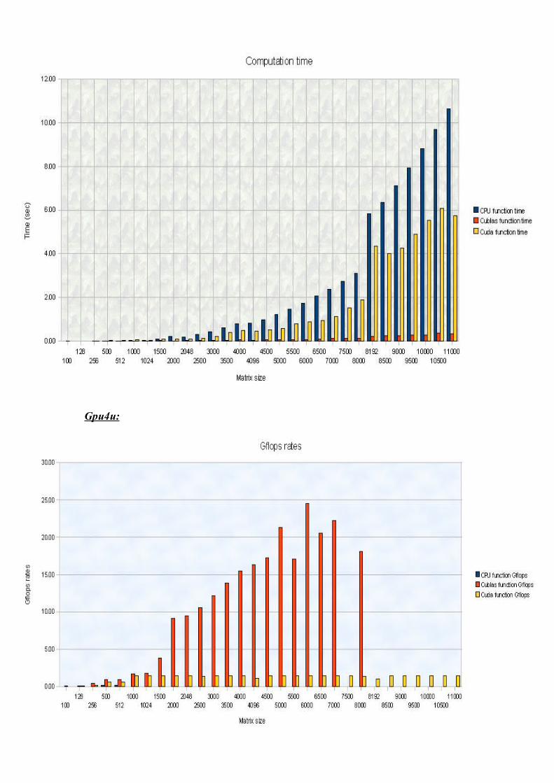
Gpu4u:
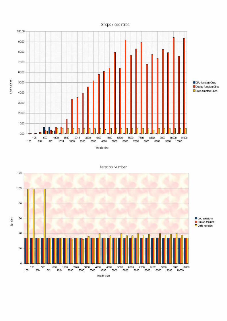
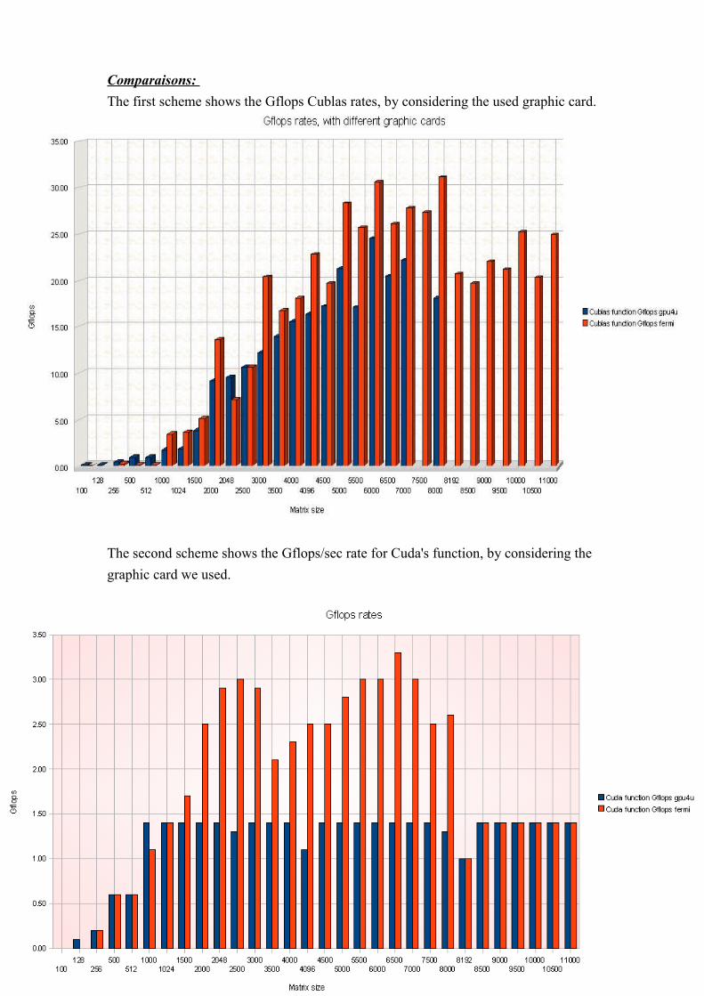
Comparaisons: The first scheme shows the Gflops Cublas rates, by considering the used graphic card.
The second scheme shows the Gflops/sec rate for Cuda's function, by considering the graphic card we used.

We can conclude that our Cuda's code is like two times better with the fermi computer. About the Cublas code, the performance is not so satisfiable.
We studied all codes we implemented to solve our linear system with Conjugate Gradient. We will now conclude on this project.
ConclusionConclusion
During my last placement in CEA, we already studied the PETSc library, and its impact on MINOS solver. We concluded that we obtained better convergences performances with PETSc, but in term of computation time, PETSc was much slower.The issue was now to study the Conjugate Gradient by using the Graphic card: to do so, we wanted to use PETSc, as we worked with it before, but also to program the Conjugate gradient with Cuda and Cublas.We concluded that Cublas offers better performances than Cuda. However, the Cuda's code is much more efficient with fermi graphic cards, than Cublas' code.Regarding PETSc, we conclude on a very good gain performance for Multigrid objects, by using GPU. The computation's time for PETSc 's code is however not so significantly different as the Megaflops rates obtained (with and without GPU).The next step is now to study our KSP code, with GPU, but to do so, it is necessary to reinstall PETSc development version. We also developed a matrix interface, which allows to load every matrix available on Matrix market website. In the future, this program will be ameliorated, and this interface will be used.

BibliographyBibliographyThesis of M. Pierre Guérin,Thesis of M. Berlier,Petsc User ManualCuda user manualCublas user manual
WebographyWebographySite de l'Idris : http://www.idris.fr/data/cours/parallel/mpi/choix_doc.htmlSite de Petsc : http://www.mcs.anl.gov/petsc/petsc-as/


![Equation Page Side 1[2]](https://img.pdfslide.us/doc/110x75/546507c6b4af9f0a328b46b5/equation-page-side-12.jpg)