Extended Kalman Filter Methods for TrackingWeak GPS Signals

Mark L. Psiaki and Hee Jung, Cornell University, Ithaca, N.Y.

BIOGRAPHIES

Mark L. Psiaki is an Associate Professor of Mechanicaland Aerospace Engineering at Cornell University. Hereceived a B.A. in Physics and M.A. and Ph.D. degrees inMechanical and Aerospace Engineering from PrincetonUniversity. His research interests are in the areas ofestimation and filtering, spacecraft attitude and orbitdetermination, and GPS technology and applications.

Hee Jung is a Ph.D. candidate in Mechanical andAerospace Engineering at Cornell University. Shereceived her BS and MS in Astronomy from the SeoulNational University in Korea and another MS inAerospace Engineering from Texas A&M University.Her main research interests are orbit and attitudedetermination of satellites with GPS applications.

ABSTRACT

A combined phase-locked loop/delay-locked loop hasbeen developed for tracking weak GPS C/A signals. Thiswork enables the use of the weak side-lobe signals thatare available at geosynchronous altitudes. The trackingalgorithm is an extended Kalman filter (EKF) thatestimates code phase, carrier phase, Doppler shift, rateof change of Doppler shift, carrier amplitude and data bitsign. It forms a likelihood function that depends on theerrors between accumulations and their predicted values.It recursively minimizes this likelihood function in orderto track the signal. It deals with data bit uncertainty usinga Bayesian analysis that determines a posterioriprobabilities for each bit sign. A second filter is used toinitialize the EKF. This batch filter starts with coarsecarrier frequency and code phase estimates and refinesthem using maximum likelihood techniques whileestimating the carrier phase and the first PRN codeperiod of a navigation data bit. The resulting system canacquire and maintain lock on a signal as weak as 15 dBHz if the receiver clock is an ovenized crystal oscillatorand if the line-of-sight acceleration variations are as mildas those seen by a geostationary user vehicle.

I. INTRODUCTION

Tracking algorithms allow a GPS receiver to maintainlock on the Doppler shift and the pseudo-random number

(PRN) spreading code of a received signal so that thereceiver can determine navigation observables anddecode the navigation data message. One necessarytracking algorithm is a delay-locked loop (DLL), whichmaintains phase alignment between the received PRNcode and a replica in the receiver. A receiver uses eithera frequency-locked loop (FLL) or a phase-locked loop toalign a replica of the carrier signal with the receivedcarrier. Various designs exist for these tracking loops,e.g., see Refs. 1 and 2.

The goal of the present work is to design a combinedDLL/PLL code and carrier tracking loop that is effectiveat tracking GPS L1 Coarse/Acquisition signals (C/A) forvery low carrier-to-noise ratios. This is to beaccomplished without prior knowledge of the navigationdata bits. These tracking loops will be developed usingoptimal estimation techniques. Standard DLLs and PLLs,while robust, are not optimal. PLLs lose lock at lowcarrier-to-noise ratios because of the nonlinearities intheir discriminators and because of dynamic variations ofthe signal's phase 2. Uncertainty about the navigation databits greatly exacerbates the problems of PLLs at lowcarrier-to-noise ratios because bit error rates becomelarge and lead to a destabilizing feedback effect. Thegoal of using optimal techniques is to deal with theseproblems in the best possible way and thereby lower thecarrier-to-noise threshold at which loss of lock occursfor a given level of signal phase dynamics.

The motivation for this work comes from a desire to useGPS for high-altitude spacecraft navigation, above theconstellation. Typical off-the-shelf receivers can tracksignals down to a carrier-to-noise density, C/N0, of about35 dB Hz, which is marginally sufficient for trackingmain-lobe signals at geosynchronous altitudes using apatch antenna. Simulation studies of high-altitudenavigation performance predict that significant gains canbe made if signals can be used effectively down to 28 dBHz 3,4. This present work aims to track signals in the 12-29 dB Hz range. This will enable the use of side-lobesignals received at geosynchronous altitudes using apatch antenna 5. Additional motivation for this workcomes from a desire to track transient weak signals thatoccur terrestrially during ionospheric scintillations 6.Such an ability would enable physicists to extract a

greater amount of information from GPS soundings ofthe disturbed ionosphere.

The present work makes three main contributions. First,it develops a new fine acquisition algorithm. Thisprocedure is needed in order to provide the trackingalgorithm with accurate initial estimates of the carrierfrequency, carrier Doppler shift, code phase, and carrieramplitude. It starts with coarse estimates of the carrierDoppler shift and the code phase and uses a batchnonlinear filter to refine these estimates while solvingfor initial carrier phase and carrier amplitude. Thepaper’s second contribution is the development of acombined carrier- and code-tracking nonlinear Kalmanfilter. A Kalman filter is an optimal algorithm that isefficient for real-time implementation because of itsiterative-in-time nature. The third contribution is aBayesian adaptation of nonlinear Kalman filteringtechniques that deals effectively with the uncertainnavigation data bits when the carrier-to-noise density islow. The new fine acquisition and tracking algorithmsare tested using a high-fidelity simulation of the weakGPS signal that exits a receiver’s RF front end.

Some of these algorithms require a special receiverarchitecture. The coarse and fine acquisitions must takeplace in a software receiver environment because theavailable algorithms for coarse acquisition of weaksignals 7 and the new algorithm for fine acquisition arebatch algorithms. The new tracking algorithm operates inan iterative causal manner using standard accumulations.It can be implemented in a software receiver or in astandard real-time receiver that uses a hardwarecorrelator. This paper envisions a system that acquiresan initial batch of data for coarse and fine acquisition.While it is processing this data, it continues to record astream of intermediate frequency data from its RF frontend for later use in tracking. After it has finished itscoarse and fine acquisition calculations, it initiates thenew weak signal tracking algorithm. It starts out trackingstored data and operates faster than real-time in order to“catch up”. Afterwards it continues to track a givensignal in real time. Systems that lack sufficient power todo batch-mode acquisition, interim RF bit storage, and“catch-up” tracking still could use the new trackingalgorithm. Its weak signal capabilities would be usefulfor a signal that suffered a power fade subsequent tohaving been acquired by standard techniques.

The remainder of this paper includes 4 main sectionsfollowed by conclusions. Section II presents models ofthe correlation measurements and the signal. Section IIIdescribes the fine acquisition algorithm. Section IVexplains the Kalman filter-based tracking algorithm.Section V presents simulation results for thesealgorithms. Section VI gives the conclusions.

II. MODELS OF THE CORRELATION MEASURE-MENTS AND THE SIGNAL DYNAMICS

The batch fine-acquisition algorithm and the signaltracking Kalman filter operate using dynamic models ofcarrier phase, code phase, and carrier amplitude andmeasurement models that give the relationship betweenthese signal quantities and the correlations that thereceiver uses to sense the signal. These models assumethat the sampled signal coming out of the receiver’s RFfront end takes the form

yj = A(τj)d[τj–ts(τj)] C[τj–ts(τj)] cos[ωIFτj-φ(τj)] + nj (1)where yj is the measured RF front-end output at sampletime τj, A(τ) is the carrier amplitude, d(τ) is the 50 Hznavigation data bit stream of ±1 values, C(τ) is the 1.023MHz C/A PRN bit stream of ±1 values, ts(τ) is the PRNcode phase expressed as a relative code start time, ωIF isthe RF front-end’s intermediate image of the nominalGPS L1 carrier frequency, φ(τ) is the carrier phase thatresults from accumulated delta range, and nj is anelement of a zero-mean discrete-time Gaussian whitenoise sequence with a variance of σn

2. The carrier-to-noise density of this sampled signal is C/N0 =A2/(4σn

2δτ), where δτ = τj+1 - τj.

Accumulation Measurement Models. The receiveraccumulates correlations between the yj data stream andreplicas of the code and carrier signals that it produces.These accumulations take the usual forms

∑ −+=+

+=−

kk

kjNCOjIFNCOkjNCOj

Nj

1jjk costCyI )]([)()( τφτω∆τ∆

(2a)=)(∆kQ

∑ −+−+

+=−

kk

kjNCOjIFNCOkjNCOj

Nj

1jjsintCy )]([)( τφτω∆τ

(2b)

where Ik(∆) and Qk(∆) are, respectively, the in-phase andquadrature accumulations with an “early” offset of ∆,which will be a late offset if ∆ < 0. The function CNCO(τ)is the receiver's reproduction of the tracked PRN code.The subscript NCO is used because this functionsimulates a code numerically controlled oscillator. Thetime tNCOk is both the NCO's prompt code start time andthe start time of the accumulation interval. The initialsample jk+1 is the minimum value that respects the boundtNCOk ≤ τjk+1. Each accumulation spans one PRN codeperiod; therefore, the number of samples Nk is themaximum value that respects the limit τjk+Nk < tNCOk+1. Thefunction φNCO(τ) is the receiver's reproduction of thesignal’s carrier phase. The negative sign in front of itpresumes high-side mixing during one of the RF front-end’s down conversion stages.

Equations (2a) and (2b) give a recipe for how the

receiver calculates its accumulations, but the fineacquisition algorithm and the Kalman filter need a modelof how these accumulations are related to the actualsignal parameters in eq. (1). This model takes the form:

Ikk ntRcos2

dANI kkmkk ++= )()()( ∆∆φ∆∆ (3a)

Qkk ntRsin2

dANQ kk

mkk ++−= )()()( ∆∆φ∆∆ (3b)

where kA is the average carrier amplitude over theaccumulation interval, dm is the navigation data bit, ∆φk isthe interval average of the carrier phase errorφ(t)–φNCO(t), ∆tk = ts(tmidk)-tmidk is the code phase error at theinterval mid-point tmidk = (tNCOk+tNCOk+1)/2, R(t) is theautocorrelation function of the PRN code, and nIk and nQk

are samples of zero-mean, uncorrelated Gaussiandiscrete-time white noise sequences, both with varianceequal to Nkσn

2/2. The model of R(t) that gets used has theslope discontinuities of its triangular peak rounded off bycubic splines. These cause d2R/dt2 to be continuous,which avoids problems in the gradient-based numericaloptimizations that are part of the fine acquisitionalgorithm and the Kalman filter. This modification ofR(t) is reasonable because the limited bandwidth of theRF front end rounds off the actual correlation’s sharpcorners.

The Kalman filter make use of prompt and early-minus-late accumulations that are summed over entirenavigation data bit periods. These form the 4×1measurement vector

∑ −−

∑ −−

∑

∑

=

+

=

+

=

+

=

+

=

19

19

19

19

)]()([

)]()([

)(

)(

21

1

1

m

meml

m

meml

m

m

m

m

k

kkemlkemlk

k

kkemlkemlk

k

kkk

k

kkk

mnm

2/Q2/Q

2/I2/I

0Q

0I

Ny

∆∆

∆∆σ

η

η

(4)where m is the index of the navigation data bit interval, Nm

= (Nkm +Nkm+1 + …+ Nkm+19) is the number of RF front-endsamples in the data bit interval, km is the index of the firstPRN code period of the data bit interval, ∆eml is the timeoffset between the early and late versions of thereceiver’s PRN code reconstruction, and ηeml =2[1-R(∆eml)] is a constant. Equation (4) gives a recipe forhow to compute ym from receiver data, but the Kalmanfilter also requires a model of how ym is related to signalparameters. It takes the form:

ym

memlm

memlmm

nm n

tRins

tRcos

tRsintRcos

NdAy

eml

eml

mm

mm

mm +

−

=

− )()(

)()(

)()()()(

21

1

∆φ∆

∆φ∆

∆φ∆∆φ∆

σ

η

η

= dm hm(∆φm,∆tm, mA ) + nym (5)

where mA is the average carrier amplitude over the bitinterval, ∆φm is the average carrier phase error over thebit interval, ∆tm = ts(tmidm)-tmidm is the code phase error atthe mid-point of the bit interval tmidm = (tNCOkm+tNCOkm+20)/2,Reml(∆t) = R(∆t+∆eml/2)-R(∆t-∆eml/2) is the early-minus-late correlation function, and nym is a sample from a zero-mean, uncorrelated Gaussian discrete-time white noisevector sequence with covariance equal to the 4×4 identitymatrix. Equations (4) has been specifically designed inorder to achieve this normalization of the nym

measurement error covariance.

When performing optimal estimation it is best to modelthe raw measurements and their errors statistically and touse those models directly in the design of the estimator.One should avoid ad-hoc processing of measured dataprior to statistical analysis, which is why discriminatorsare not used here. This paper’s approach, however, is inslight violation of this principle. The rawest form of themeasurements is given in eq. (1). The new algorithms donot work directly with eq. (1) because their optimization-based techniques would require many re-calculations ofcorrelations, which would be inefficient. Also, the PRNcode function C(t) is not everywhere differentiable,which would cause problems for these gradient-basedoptimization procedures. This "impure" approach doesnot cause significant loss of performance because of thefollowing facts: The measurements in eqs. (2a), (2b),and (4) capture almost all of the important informationabout the signal, the measurement models in eqs. (3a),(3b), and (5) are faithful, and the noise in thesemeasurements remains Gaussian.

Carrier Phase, Code Phase, and Carrier AmplitudeDynamic Models. The carrier phase dynamics modeltakes the form of a discrete-time triple integrator drivenby discrete-time white noise:

1kxxx

+

α

ω

φ =

10010

21

k

2k

k

t

tt

δ

δδ

kxxx

α

ω

φ -

00ktδ

ωNCOk

+

010000100001

wφk (6)

where xφk = φ(tNCOk) – φNCO(tNCOk) is the difference betweenthe true carrier phase and the receiver NCO’s carrierphase at the start of an accumulation interval, xωk is thetrue carrier Doppler shift at the start of the interval, xαk isthe rate of change of the carrier Doppler shift at the startof the interval, ωNCOk is the receiver NCO’s reconstructedcarrier Doppler shift for the interval, δtk = tNCOk+1 - tNCOk isthe length of the interval, and wφk is a member of a zero-mean, discrete time Gaussian white-noise vectorsequence. The states of this model can be used to deducethe average carrier phase error over the accumulationinterval:

∆φk =

621

2kk tt δδ

kxxx

α

ω

φ-

2ktδ ωNCOk + [ ]1000 wφk

(7)This quantity is needed in eqs. (3a) and (3b). A similarcarrier phase model applies when accumulations getsummed over bit intervals, as in eq. (4). In this case, thek index of the PRN code period in eqs. (6) and (7)changes to the m index of the data bit period, and thenominal accumulation interval increases from δtk =0.001 sec to δtm = 0.020 sec.

The covariance of the wφk white-noise sequence is acombination of three terms. One models a random walkacceleration of the line-of-sight (LOS) vector to the GPSsatellite, as in Ref. 8, and the other two model the effectsof receiver clock phase random walk and frequencyrandom walk, as in Ref. 9. The wφk covariance takes theform:

Pwφwφk = E{ Tkk ww φφ } =

qLOS

252243072242630238726820

5k

3k

4k

5k

3kk

2k

3k

4k

2k

3k

4k

5k

3k

4k

5k

tttttttttttttttt

δδδδδδδδδδδδδδδδ

+ SgωL12

200680000

6028023

3k

2k

3k

2kk

2k

3k

2k

3k

ttt

tttttt

δδδ

δδδδδδ

+ SfωL12

300200000000

200

kk

kk

tt

tt

δδ

δδ

(8)

The quantity qLOS is the intensity of the accelerationrandom walk. Sg and Sf are the receiver clock's frequencyand phase random walk intensities, respectively 9, and ωL1

is the nominal L1 carrier frequency.

The dynamic model of the PRN code phase propagatesthe code start time from the beginning of one codeperiod to the next:

[ ]tsk

kk1L

k1Lsk1sk w

xtx

wttt

nom

nom+=+ ++

−+

αω

φ

δω

δω

0.5

0001(9)

where tsk and tsk+1 are the true start and stop times of thePRN code period in question. This model includescarrier aiding via the second term on the right-hand sideof eq. (9). The time increment δtnom is the nominal codeperiod, 0.001 sec. The scalar wtsk is a white-noisesequence that effectively models code-carrierdivergence as a random walk. Its variance is E{wtsk

2} =δtkqts, where qts is the random walk intensity. The PRNcode start/stop times in eq. (9) can be used to calculatethe code phase error ∆tk that is used in eq. (3a) and (3b):

∆tk = (tsk+1 + tsk)/2 - tmidk

= [ ]

tskkk1L

k1Lsk w

xtx

wtt

nom

nom21

21

0.5

0001+

++

−+

αω

φ

δω

δω -tmidk (10)

A model similar to eqs. (9) and (10) applies forpropagation of the navigation data bit start/stop timesfrom one bit to the next. In this case, the time index kgets replaced by the time index m, and the interval δtnom

increases to 0.020 sec.

A random walk is used to model the dynamics of thecarrier amplitude:

Akk1k wAA +=+ (11)

Ak and Ak+1 are the carrier amplitudes at the times tNCOk andtNCOk+1. The scalar wAk is the zero-mean, white-noiseGaussian sequence that drives the random walk. Itsvariance is E{wAk

2} = δtkqA, where qA is the random walkintensity. The amplitudes in eq. (11) can be used tocompute the average amplitude that is needed in eqs. (3a)and (3b):

2)( /AAA k1kk += + = Akw5.0Ak + (12)

Equations (11) and (12) can be modified to propagate thecarrier amplitude from one navigation data bit start timeto the next. The only necessary change is to switch fromthe PRN code period index k to the data bit index m.

III. BATCH FINE ACQUISITION ALGORITHM

The Kalman filter tracking algorithm of this paper needsan accurate initialization in order to function properly ina weak signal environment. The initialization procedurestarts with the usual search in code-phase/carrier-Doppler space. For purposes of the present paper, thissearch is called the coarse acquisition. A suitable batchcoarse acquisition algorithm that works well in a weaksignal environment is described in Ref. 7. This algorithmgives Doppler shift to an accuracy of about ± 6 Hz andcode phase to an accuracy of ± 0.1 chips.

The Kalman filter tracker needs the initial Doppler shiftto an accuracy about 0.25/τPLL Hz, where τPLL is thecharacteristic settling time of the filter. This time can beon the order of 1 sec when tracking a weak signal withslow dynamics. In addition, the Kalman filter needs toknow the PRN code period that corresponds to the starttime of a navigation data bit, it needs an initial carrierphase estimate that is accurate to within ± 45o, and itneeds initial estimates of the carrier amplitude and therate of change of Doppler shift. The Kalman filter alsoneeds a covariance matrix for the initial estimationerrors in its 5 states.

A sequence of fine acquisition calculations is used todetermine suitable values for the Kalman filterinitialization. The first calculation determines thenavigation data bit start time. The second calculationestimates initial values for the three carrier phase states,xφ, xω, and xα, and it uses these estimates to get a firstestimate of the carrier amplitude, A. The finalcalculation refines the estimates of these 4 quantitiesalong with the estimate of the initial code phase, ts.

Open-Loop Accumulation Data Used in Fine AcquisitionCalculations. The first step in the fine acquisition is tocalculate an “open-loop” time history of 1000 Hzaccumulations. This computation uses the Doppler shiftand code phase estimates from the coarse acquisition,ωNCO and tNCO0, to specify an “open-loop” carrier phasetime history via the formula φNCO(t) = ωNCOt and an “open-loop” code phase time history via iteration of thedifference equation tNCOk+1 = tNCOk + 0.001ωL1/(ωL1+ωNCO).These phase time histories are used to generate in-phaseand quadrature prompt and early-minus-lateaccumulations using the formulas in eqs. (2a) and (2b).Let the prompt accumulations be Ipk = Ik(0) andQpk = Qk(0), and let the early-minus-late accumulationsbe Iemlk = Ik(∆eml/2) - Ik(-∆eml/2) and Qemlk = Qk(∆eml/2) -Qk(-∆eml/2). These quantities constitute the data that getused throughout the remainder of the fine acquisitioncalculations. They are calculated for k = 0, …, Nacq. Nacq

is normally chosen to equal the number of PRN codeperiods used during the coarse acquisition.

Determination of the Start Time of a Navigation Data Bit.The objective of the bit start time calculation is todetermine the value of k0, the PRN code period indexwhose start time is also the start time of the firstnavigation data bit. The true value k0 is an element of theset {0,1,2,…,19}. It can be determined by an integeroptimization 1.

The merit function that gets optimized is the signalpower after summing over a pre-detection interval of 1navigation data bit:

∑

∑+

∑=

=

++

+=

++

+=

M

m

mk

mkkpkN

mk

mkkpkN0

0

0m

0

0m

QIkJ0

21920

20

12

1920

20

1)(

(13)where M is the maximum integer that respects the boundM ≤ (Nacq-38)/20. M+1 is the number of full data bitintervals. The integer Nm is the total number of RF front-end samples during a proposed navigation data bitinterval, as in eq. (4). It normalizes the differentsummations.

The bit start-stop determination is a brute-forceoptimization of J(k0). All 20 possible values of k0 aretried, and the value that yields the largest J(k0) getschosen as the correct bit start/stop index. If M is largeenough, then this method is very likely to yield thecorrect data bit start/stop time. If M is not very large,then one can increase M after the acquisition by using theaccumulations from the subsequent tracking interval.This approach further increases the likelihood of gettingthe correct value of k0, which is needed to calculate codepseudorange.

Batch Fine Acquisition Cost Functions. The batchacquisition calculations make use of several differentcost functions that are related to the joint probabilitydensity function of the noise terms in eqs. (3a) and (3b)or (5). The ultimate cost function that the initialestimates xφ0, xω0, xα0, A0, and ts0 must minimize isJa(xφ0,xω0,xα0,A0,ts0) =

∑

∑

++

=

++

+=

M

m

mk

mkkk

0kpkpk

k

0

0ntRANQI

N0

1920

20

222

221 )(4

12 ∆

σ

- ∑ ∑=

++

+=

M

m

mk

mkkk0

0

0ntRAcoshln

0

1920

20

1 )(2 [2{( ∆σ

})])}()({ kpkkpk sinQcosI φ∆φ∆ −

+ ∑ ∑ +=

++

+=

M

m

mk

mkkemlkemlk

k

0

0emlnQI

N0

1920

20

221 [{ 12ησ

]})(4

222

keml0k tR

AN∆+

- ∑ ∑=

++

+=

M

m

mk

mkkkeml0

0

0emlntRAcoshln

0

1920

20

1 )(2 [2{( ∆ησ

})])}()({ kemlkkemlk sinQcosI φ∆φ∆ − (14)

This cost function is a negative log likelihood function.In other words, Cexp[-Ja(xφ0,xω0, xα0,A0,ts0)] is the jointprobability density function for the four accumulationtime histories Ipk, Qpk, Iemlk, and Qemlk for k = k0 to(k0+20M+19) conditioned on the 5 unknown parametersxφ0, xω0, xα0, A0, and ts0, where C is a normalizing constant.The ln[2cosh()] terms are the results of probabilitysummations over the uncertain data bits dm under the

assumption that the +1 and –1 values are equally likely.The dependence of Ja on xφ0, xω0, and xα0 comes partlythrough the carrier phase model in eq. (6), but with wφk

set to 0 because the batch filter does not considerprocess noise. This yields the model ∆φk(xφ0,xω0,xα0) =[xφ0 +xω0(tmidk-tNCOk0) +0.5xα0(tmidk-tNCOk0)2 -ωNCOtmidk]. Thedependence of Ja on ts0 comes through the ∆tk terms.They can be computed as functions of xω0, xα0, and ts0 byiterating eq. (9) with wφk and wtsk both set zero. Thisiteration generates the time series tsk(xω0,xα0,ts0) for k = k0

to (k0+20M+19), and eq. (10) yields ∆tk(xω0,xα0,ts0) =[tsk+1(xω0,xα0,ts0)+tsk(xω0,xα0,ts0)]/2 - tmidk.

An approximation to the cost function in eq. (14) isuseful for estimating the carrier phase parameters xφ0, xω0,and xα0 and the carrier amplitude A0. It presumes that thecode phase is correct, which implies that ∆tk = 0, Reml(∆tk)= 0, and R(∆tk) = 1. This approximation makes the lasttwo summations of Ja constant, and therefore irrelevantto any optimization. An additional approximationsubstitutes the absolute value function for the ln[2cosh()]function. Use of the absolute value function amounts to“hard” bit estimation, in which the bit sign is set equal tothe sum over the data bit interval of Ipkcos(∆φk) –Qpksin(∆φk). The cost function approximation isJb(xφ0, xω0, xα0, A0) =

∑

∑

++

=

++

+=

M

m

mk

mkk

0kpkpk

k

0

0n

ANQIN0

1920

20

22221

41

2σ

- [ ]∑ ∑ −=

++

+=

M

m

mk

mkkkpkkpk0

0

0nsinQcosIA

0

1920

20

1 )()(2 φ∆φ∆σ

+ constant (15)The above cost function is quadratic in A0. It can beminimized by first minimizing the following costfunctionJc(xφ0, xω0, xα0) =

- [ ]∑ ∑ −=

++

+=

M

m

mk

mkkkpkkpk

0

0

sinQcosI0

1920

20)()( φ∆φ∆ (16)

with respect to xφ0, xω0, and xα0. One then computes A0 =-2Jcmin/Ntot to optimize Jb in eq. (15), where Ntot = Nk0 +Nk0+1 +…+ Nk0+20M+19.

Yet another cost function needs to be defined in order todeal with the fact that the cost function in eq. (16) hasmany local minima. A search on a grid has to beperformed in order to find the global minimum, and analternate cost function allows a reduction from a 3-dimensional grid to a 2-dimensional grid. The alternatecost function is

Jd(xφ0, xω0, xα0) =

[ ]∑

∑ +=

++

+=

M

m

mk

mkkkpkkpk

m

0

0

cosQsinIN0

21920

20)()(1 φ∆φ∆

(17)This cost function is a weighted sum of the norm squaredof the projection of the first two elements of themeasurement error vector nym of eq. (5) perpendicular tothe signal direction. The importance of this costfunction is that it can be minimized with respect to xφ0

analytically, which reduces the dimensionality of thesearch grid over which one must seek the globalminimum. In order to minimize Jd with respect to xφ0,defineIrm(xω0, xα0) =

[ ]∑ −−−++

+=

1920

20)()(

mk

mkk0kpk0kpk

0

0

xsinQxcosI φφ φ∆φ∆ (18a)

Qrm(xω0, xα0) =

[ ]∑ −+−++

+=

1920

20)()(

mk

mkk0kpk0kpk

0

0

xcosQxsinI φφ φ∆φ∆ (18b)

where the r subscript of the accumulations stands for"rotated". Neither of these accumulations depends on xφ0

because ∆φk-xφ0 is independent of xφ0, and the value of xφ0

that minimizes Jd for given values of xω0 and xα0 isxφ0opt(xω0, xα0) =

-

∑

−

∑

==

M

m m

rmrmM

m m

rmrmN

QI,N

QI2tana0

22

021 ][2 (19)

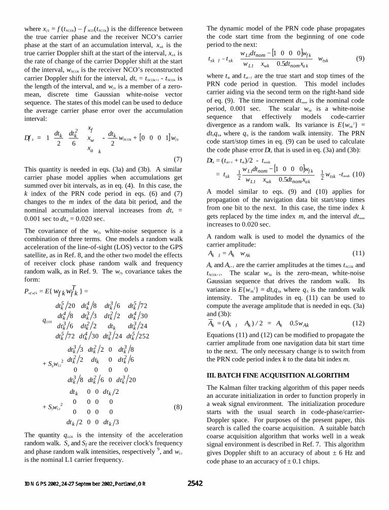
A Sequence of Fine Acquisition Optimizations. The firststep in the fine acquisition algorithm is an approximateglobal minimization of Jc(xφ0,xω0,xα0). This proceduresearches for the minimum on a grid in (xω0,xα0) space andcomputes xφ0 at each grid point by using eq. (19). Figure1 explains why the phase xφ0 that minimizes Jd will be agood approximation to the phase that minimizes Jc. Thefigure plots the rotated accumulations Ipsin(∆φ)+Qpcos(∆φ) on the vertical axis versus Ipcos(∆φ)-Qpsin(∆φ) on the horizontal axis for a case in which xω0

and xα0 are nearly correct. The minimization of Jc withrespect to xφ0 performs an additional rotation in order tomaximize the spread of these points along the horizontalaxis, which would tend to align the solid line with thehorizontal axis. The minimization Jd, rotates xφ0 in orderto minimize the spread of these points along the verticalaxis, which would tend to align the dash-dotted line withthe vertical axis. Thus, these two minimizations tend toproduce nearly the same optimal xφ0 rotation, which iswhy the eq. (19) value of xφ0 can be used to approximatelyoptimize Jc(xφ0, xω0, xα0).

The extent and spacing of the search grid in (xω0,xα0) spacemust be chosen carefully in order to get a good solution.

The xω0 grid should be centered at the coarse acquisitionDoppler shift estimate, and it should extend in eitherdirection as far as the possible uncertainty in the coarseDoppler shift. A good rule of thumb is to extend for±25% of the pre-detection bandwidth of the coarseacquisition or ±100% of the Doppler grid spacing of thecoarse acquisition, whichever is greater. For most of theexamples of this paper a range of ±12.5 Hz has beenused. The xα0 grid should be centered at zero. Recall thatxα0 models acceleration. The extent of this grid should bechosen to reflect the range of possible LOSaccelerations. For a geosynchronous receiver, the LOSacceleration comes mainly from gravitation and rangesup to 0.081 g, which translates into xα0 = 26.3 rad/sec2

(4.2 Hz/sec). The actual search should expand to includea factor of safety which ensures that the global minimumdoes not fall outside of the grid. A range of ±33.6rad/sec2 (±5.3 Hz/sec) has been used in the present study.

Fig. 1. Relationship of in-phase and quadratureaccumulations to cost functions Jc and Jd, an18 dB Hz example.

The required xω0 and xα0 grid spacings vary inversely withthe length of the batch interval, Tfine = 0.020(M+1). Thelimits ∆xω0 ≤ π/(2Tfine) and ∆xα0 ≤ π/(Tfine

2) ensure that theworst-case error between the true optimum and theclosest (xω0,xα0) grid value yields no more than a quartercycle of erroneous I/Q rotation over the data batch. Thisbound on the erroneous rotation prevents theaccumulations shown in Fig. 1 from being spun into acircular distribution that washes out the two distinct I/Qclouds whose detection is of central importance to phaseestimation. For a typical batch duration of 3 seconds,these limits translate into a grid of 300 frequency pointsby 200 frequency-rate points, or 60,000 total points.

The second step of the fine acquisition algorithmcomputes the exact global minimum of Jc(xφ0,xω0,xα0). It

does this using Newton's method. It starts with the 10lowest isolated minima of Jc[xφ0opt(xω0,xα0), xω0, xα0] at thegrid points of the previous calculation and performs aniterative Newton search from each point in order tooptimize Jc with respect to xφ0, xω0, and xα0. The guardedNewton search includes precautions that ensure globalconvergence to a local minimum, such as modification ofthe cost Hessian and adaptation of the search step size 10.The point that achieves the lowest minimum usingNewton's method yields fine estimates for the carrierphase, xφ0, the Doppler shift, xω0, and the Doppler shiftrate, xα0. Ten different initial guesses are used in order toincrease the likelihood that one of the first guesses willreach the true global minimum of Jc.

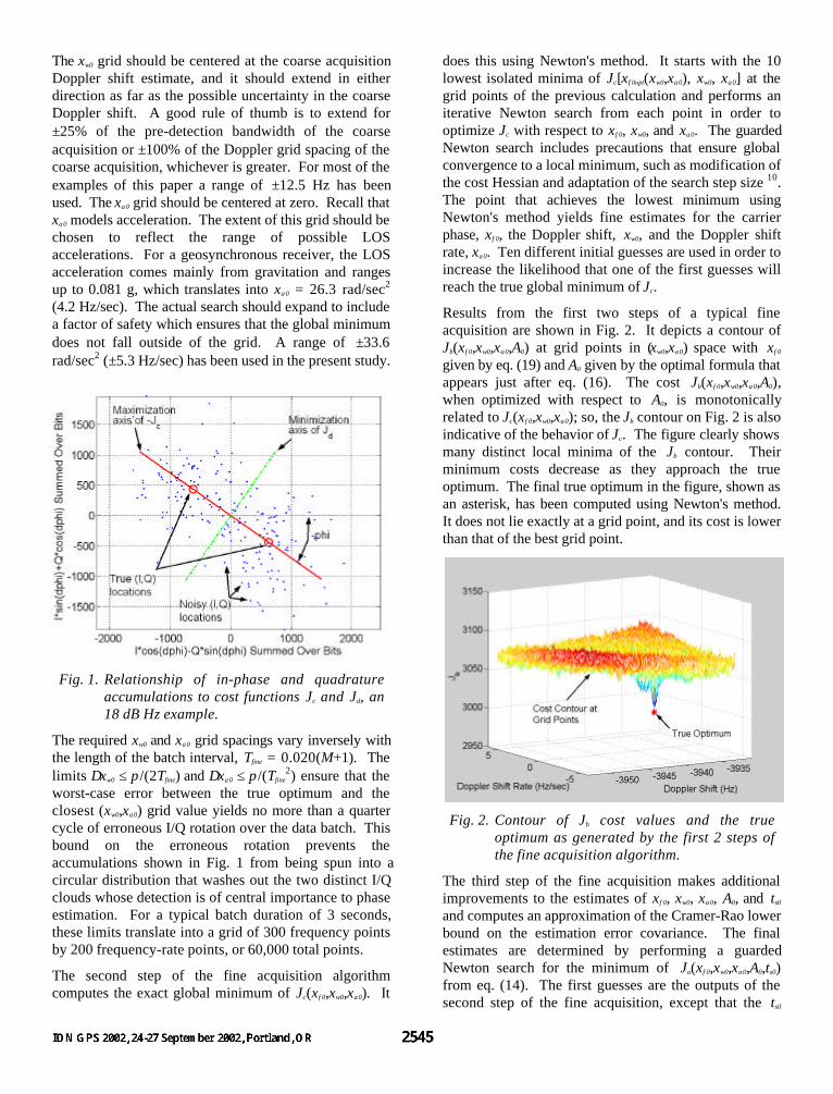
Results from the first two steps of a typical fineacquisition are shown in Fig. 2. It depicts a contour ofJb(xφ0,xω0,xα0,A0) at grid points in (xω0,xα0) space with xφ0

given by eq. (19) and A0 given by the optimal formula thatappears just after eq. (16). The cost Jb(xφ0,xω0,xα0,A0),when optimized with respect to A0, is monotonicallyrelated to Jc(xφ0,xω0,xα0); so, the Jb contour on Fig. 2 is alsoindicative of the behavior of Jc. The figure clearly showsmany distinct local minima of the Jb contour. Theirminimum costs decrease as they approach the trueoptimum. The final true optimum in the figure, shown asan asterisk, has been computed using Newton's method.It does not lie exactly at a grid point, and its cost is lowerthan that of the best grid point.

Fig. 2. Contour of Jb cost values and the trueoptimum as generated by the first 2 steps ofthe fine acquisition algorithm.

The third step of the fine acquisition makes additionalimprovements to the estimates of xφ0, xω0, xα0, A0, and ts0

and computes an approximation of the Cramer-Rao lowerbound on the estimation error covariance. The finalestimates are determined by performing a guardedNewton search for the minimum of Ja(xφ0,xω0,xα0,A0,ts0)from eq. (14). The first guesses are the outputs of thesecond step of the fine acquisition, except that the ts0

guess is taken from the coarse acquisition. This searchconverges rapidly, normally in 3-10 iterations. Theapproximate Cramer-Rao estimation error covariance isthe inverse of the Hessian of the Ja cost function at thefinal optimum, Pxx0 = [∂2Ja/∂x2]-1, where x is the 5x1vector [xφ0,xω0,xα0,A0,ts0]T .

Mid-Point Calculations for Kalman Filter Initialization.The fine acquisition algorithm's carrier phase andDoppler shift estimates have their highest accuracy at themid-point of the acquisition batch interval. Therefore,the estimates at the mid point are used to initialize thetracking Kalman filter. The value mc = round(M/2) is theindex of the navigation bit whose start time is nearest tothe midpoint of the fine acquisition batch interval. Thestart time of this bit is tNCOk0+20mc, and ∆tc = tNCOk0+20mc - tNCOk0 isthe time offset of the midpoint from the start of the fineacquisition batch interval. The Kalman filter initializes attime tk0+20mc using the initial state estimate[(xφ0+∆tcxω0+0.5∆tc

2xα0),(xω0+∆tcxα0), xα0,A0,tsc]T , where tsc isthe estimated start time of the mid-point navigation databit as determined by iteration of eq. (9) with zeroprocess noise. The covariance gets propagated to thistime point using the following formula:

Pxxc = TPxx0TT , where T =

10000010000010000100021 2

c

cc

ttt∆

∆∆

(20)

This propagation neglects the effects of xω0 and xα0

uncertainty on tsc, which is reasonable because of theirsmall magnitude.

IV. AN EXTENDED KALMAN FILTER FORCARRIER AND CODE TRACKING

The extended Kalman filter tracking algorithm is astraight-forward implementation of Kalman filteringprinciples, except for two points. First, it uses aBayesian integration process to deal with the uncertaindata bits. Second, it uses nonlinear iteration in asomewhat unconventional way during its measurementupdate. The first part of this section describes how theKalman filter operates when the navigation data bit signis assumed to be known. The second part explains how aBayesian analysis deals with data bit uncertainty bymixing the different estimates that result from differentassumptions about data bit signs.

Iterated Extended Kalman Filter with Assumed Bit Signs.The iterated extended Kalman filter performs a singlemeasurement update and state propagation over a singledata bit interval by solving the following weighted leastsquares problem:

find: xm, xm+1, and wm (21a)to minimize:

J = 21 [ )( mmxxm x~xR~ − ]T[ )( mmxxm x~xR~ − ]

+ )()( T21

mwwmmwwm wRwR

+ )],(-[)],(-[ T21

mmmmmmmmmm wxhdywxhdy

(21b)subject to:

xm+1 = fm(xm,wm) (21c)where the unknown solution vectors are the state xm =[xφm,xωm,xαm,Am,tsm]T and the process noise wm =[wφm

T ,wtsm,wAm]T . The known data bit value is dm. Themeasurement function hm(xm,wm) is effectively defined byeq. (5) with eqs. (7), (10), and (12) used to substitute for∆φm, ∆tm, and mA in terms of xm and wm. The discrete-timedynamics function fm(xm,wm) is effectively defined by eqs.(6), (9), and (11). It is linear except for the carrier aidingterm in the tsm iteration, eq. (9), and the nonlinear term inthat equation can be well approximated by a linear modelbecause ωL1 is much larger than the Doppler shift.

The vector mx~ is the a priori estimate of xm based on allof the accumulations up through data bit interval m-1, thematrix xxmR~ is the corresponding a priori estimationerror square root information matrix, and the matrix

wwmR is the a priori process noise square rootinformation matrix. The corresponding a prioricovariances are related to these matrices as follows: Pxxm

= T1 −−xxmxxmR

~R~

and Pwwm = T1 −−wwmwwmRR , where the notation

()-T refers to the inverse transpose of the matrix inquestion. Note that mx~ and xxmR~ correspond to thebatch fine acquisition algorithm's mid-interval estimatefor m = 0, and they are determined by the previousiteration of the Kalman filter for m > 0. wwmR isdetermined from Pwwm, which is defined by the variousprocess noise covariances already given in eq. (8) and inthe text sections that follow eqs. (9) and (11) and by thefact that wφm, wtsm, and wAm are uncorrelated.

The Kalman filter solution procedure first minimizes thecost function in eq. (21b) with respect to xm and wm, andthen it uses eq. (21c) to propagate the solution to xm+1.The minimization in eq. (21b) is an iterative Newtonminimization that is guarded in order to ensureconvergence. This differs from a conventional iterativeKalman filter because it uses step-size adaptation toensure convergence to a local minimum of a weightedleast-squares cost function.

The Hessian matrix of the cost function in eq. (21b),which is required for Newton's method and forcalculation of 1xxmR~ + , is computed and stored in square

root form. This procedure first computes the upper-triangular square root of the Gauss-Newtonapproximation of the Hessian, RG. This calculation isperformed using QR factorization:

0G

GR

Q =

∂∂

∂∂

)()(

00

xh

dwh

d

R~

R

mm

mm

xxm

wwm

(22)

Next, the procedure calculates the exact Hessian in thefactored form RG

TDRG, where the symmetric D matrixdiffers from the identity by a term that involves thesecond derivatives of hm with respect to xm and wm. Theprocedure next attempts to Cholesky factorize D into theform RD

TRD = D. If this factorization fails because D isnot positive definite, then the Hessian square root RH getsapproximated as RH = RG. Otherwise, the Hessian squareroot is computed exactly as RH = RDRG. Standard Newtontechniques then use RH and the gradient of the costfunction to compute updates to xm and wm.

The last operation of the Kalman filter is the propagationto determine 1mx~ + and 1xxmR~ + so that the algorithm canoperate recursively starting at the next data bit interval.The solution to the optimization problem in eq. (21b),the cost Hessian evaluated at the solution, and eq. (21c)are used to do the propagation. Suppose that theestimates mx and mw minimize the cost in eq. (21b) andsuppose that the square root of the Hessian is

xxm

wxmwwmRRR

0 = RH (23)

Suppose, also, that the Jacobian of the dynamics functionin eq. (21c) is

[ ]mm ΦΓ = )( mm w,x

mmx

fwf

∂∂

∂∂

(24)

Then 1mx~ + is determined by evaluation of eq. (21c) atthe current best estimate, i.e., 1mx~ + = fm( mx , mw ), and

1xxmR~ + is computed via the following QR factori-zation 11,12:

+1xxm

wxmwwmm R~

R~R~Q

0 =

−−

−−

−−

11

11

)()(

mxxmmmxxm

mwxmmmwxmwwm

RRRRR

ΦΓΦΦΓΦ (25)

where Qm is an orthonormal matrix and wwmR~ and

1xxmR~ + are square, non-singular, upper-triangularmatrices.

The square-root Kalman filter form used in thesedevelopments is important to successful implementation

of this tracking algorithm. In theory, it would be possibleto develop a non-square root filter, but experience withthis particular problem has shown that non-square rootfilters can diverge due to the build-up of numericalround-off errors. Square root filters are specificallytailored to alleviate such problems 11.

Bayesian Treatment of Unknown Navigation Data Bits.The Kalman filter of the preceding sub-section, whichassumes that the data bit sign is known, can be used aspart of a Bayesian analysis when the bit sign is unknown.The Bayesian approach executes the filter calculationstwice, once for each possible navigation data bit sign.

Suppose that the results are )(++1mx~ and )(+

+1xxmR~ for the

assumption that dm = +1 and )(−+1mx~ and )(−

+1xxmR~ for

dm = -1. Suppose, also, that the eq. (21b) optimal costs

for these two different solutions are, respectively, )(+mJ

and )(−mJ and suppose that the a priori probabilities of +1

and –1 bit values are )(+mp = )(−

mp = 0.5. Then it can beshown that the a posterior probabilities of the +1 and –1bit values are

)(++1mp~ = )()(

)(

−+

+

+ mm

m

ρρ

ρ, )(−

+1mp~ = )()(

)(

−+

−

+ mm

m

ρρ

ρ(26)

where

)(+mρ = }][{

)(

)( )()()()(

)(+−+

++

+

− mmm1xxm

xxmmJJ,Jminexp

R~det

R~

detp

(27a)

)(−mρ = }][{

)(

)( )()()()(

)(−−+

−+

−

− mmm1xxm

xxmmJJ,Jminexp

R~det

R~

detp

(27b)The derivation of these formulas uses the conditionalprobability density function for xm given themeasurements and the bit sign assumption. Thisprobability density equals Cexp(-J), where C is anormalizing constant and J is the cost from eq. (21b).The derivation approximates J by a quadratic expansionabout its minimum. The leading term in the exponential

argument in eqs. (27a) and (27b), ][ )()( −+mm J,Jmin , is not

needed in theory, but it is useful in practice as a means ofavoiding computer overflow or underflow problems.

One can see from eqs. (26)-(27b) that the optimal cost isthe important factor in determining the a posterioriprobabilities of the two bit signs. All other things beingequal, the bit sign assumption that produces the smallestoptimal cost in eq. (21b) will have the highest aposteriori probability. This makes intuitive sensebecause it gives preference to the bit sign whosecorresponding a priori expected measurement is closest

to the actual measurement.

The probabilities in eq. (26) can be used to "mix" the twoestimates and their square-root information matrices toproduce the expected state and the covariance of theestimation error in the expected state. This mixingpresumes that the estimation error distributions for thetwo bit sign assumptions are Gaussian. The mixed valuesare:

1mx~ + = )(++1mp~ )(+

+1mx~ + )(−+1mp~ )(−

+1mx~ (28a)

1mP~ + = )(++1mp~ [ )(+

+1mP~ + ( )(++1mx~ - 1mx~ + )( )(+

+1mx~ - 1mx~ + )T]

+ )(−+1mp~ [ )(−

+1mP~ + ( )(−+1mx~ - 1mx~ + )( )(−

+1mx~ - 1mx~ + )T]

(28b)Thus, the mixed state estimate is a simple weighted sumof the two state estimates. The mixed covarianceestimate includes a weighted sum of the two covariances,but it also includes terms that increase the covariance inthe directions from the mixed estimate to the estimatesthat apply if one or the other bit sign assumption iscorrect. This makes sense because one or the other ofthese estimates would be the best one if the bit sign wereknown, which increases the uncertainty in thesedirections. Of course, if one of the a posterioriprobabilities is very near 1, then the mixed state estimateand covariance are very nearly equal to the state estimateand the covariance for that bit sign assumption

A square-root information version of eq. (28b) has beendeveloped. The square root mixing method uses QRfactorization to calculate the square, non-singular, upper-triangular matrix Rmix and the orthonormal matrix Qmix thatsatisfy the following relationship:

[ ] mixmix QR 0 = K,x~x~R~,I 1m1m1xxm }{ )()([ +++

++ −

K,R~R~ 1xxm1xxmp~p~

1m

1m 1)()( }{)(

)(−−

++

+++

−+

]}{ )()()(

)(

1m1m1xxmp~

p~x~x~R~

1m

1m+

−+

++ −

++

−+ (29)

The following formula then gives the mixed square-rootinformation matrix:

1xxmR~ + = )(11)(

++

−++

1xxmmixp~

R~R1m

(30)

The preceding calculations presume that )(++1mp~ ≥ )(−

+1mp~ .

If )(++1mp~ < )(−

+1mp~ , then eqs. (29) and (30) get modified

by interchanging the (+) and (-) superscripts.

These Bayesian calculations are critical to the successfuloperation of the tracking Kalman filter at low carrier-to-noise densities. It can become difficult to determine bitsigns exactly when the signal is weak. Consider Fig. 1.

Bit signs in this example are estimated according towhich side of the dash-dotted line each (I,Q) point lieson. One can see that the signs of a number of bits will bemis-identified because the two clouds of (I,Q) pointsintersect. This intersection is the defining characteristicof the low carrier-to-noise density case. If there is acarrier phase error, then (I,Q) points near the separatingline tend to get mis-identified in a biased way that candestabilize a PLL. The Bayesian method de-weights such

(I,Q) combinations because their )(++1mp~ and )(−

+1mp~ values

tend to be nearly equal. This de-weighting helps tocounteract the destabilizing effect of systematic bit mis-identification.

There are other possible algorithms for dealing with theuncertain navigation data bits. A number of them weretried before the Bayesian method was developed. Onemethod chose dm based on which value gave the lowesteq. (21b) cost at xm = mx~ and wm = 0. Another methodmade a "soft" bit sign decision by including an ln[2cosh()]term in the measurement error part of eq. (21b). Neitherof these methods performed as well as the Bayesianmethod. They all suffered from a propensity to make toodefinite of a decision about the correct bit sign when the(I,Q) point was near the sign boundary as determinedfrom the imperfect carrier phase estimate.

Explicit Multi-Bit Bayesian Analysis. It is possible toextend the analysis of the previous sub-section to dealwith multiple data bits in a Bayesian manner. Supposethat Nb is the total number of data bits whose signs areexplicitly allowed to vary in the Bayesian analysis. Bothpossibilities for the current navigation data bit sign areconsidered along with both possibilities for the mostrecent Nb-1 navigation data bits. Each of the 2Nb-1

different possible combinations of these recent bitsgives rise to an a priori state estimate and an estimation

error information matrix, )(imx~ and )(i

xxmR~

for i = 1,…,2Nb-1, and each of these estimates has an a priori

probability associated with it, )(imp~ .

The estimation procedure computes 2Nb Kalman filterestimates and square-root information matrices along

with their probabilities, )( ++,i

1mx~ , )( ++

,i1xxmR~ and )( +

+,i

1mp~ for i =

1,…, 2Nb-1, and )( −+,i

1mx~ , )( −+

,i1xxmR~ and )( −

+,i

1mp~ for i = 1,…, 2Nb-1.

In this formulation )( j,i1mx~ + , )( j,i

1xxmR~ + and )( j,i1mp~ + are the

Kalman filter state, the square-root information matrix,and the associated a posteriori probability under theassumptions that the correct a priori state variable

estimate is represented by [ )(imx~ , )(i

xxmR~

] and that thecorrect current bit sign is dm = j. The a posterioriprobabilities of the different cases are calculated using

modified versions of eqs. (26)-(27b): The sum in thedenominator of eq. (26) is taken over all 2Nb ρ values, theformulas for ρ in eqs. (27a) and (27b) get multiplied by

)(imp~ , the term | )( xxmR~det | in eqs. (27a) and (27b)

changes to | )( )(ixxmR

~det |, and the minimal cost in the

exponentials in eqs. (27a) and (27b) is taken over all 2Nb

cases. Equations (28a) and (28b) also change in themulti-bit formulation. They compute weighted sumsover all 2Nb cases, and there is a corresponding change tothe square-root information matrix update in eqs. (29)and (30).

This approach requires an additional mixing operation inorder to eliminate explicit consideration of the oldest

data bit. Suppose that )(imx~ , )(i

xxmR~

, and )(imp~ correspond

to one particular set of assumptions about the previous

Nb-1 data bit signs, and that 1)( +imx~ , 1)( +i

xxmR~

, and 1)( +imp~

corresponds to identical assumptions except that the signof the oldest data bit is reversed. Then the pair of

solutions [ )( ++,i

1mx~ , )( ++

,i1xxmR~ , )( +

+,i

1mp~ ] and [ )1( +++

,i1mx~ ,

)1( +++,i1xxmR~ , )1( ++

+,i

1mp~ ] needs to get combined in order to

keep the number of solutions from growing. This mustbe done for all pairs whose only difference of bit signassumption is in the oldest bit. Each such pair getsmixed using eqs. (28a) and (29), except the mixingprobabilities used in those equations are

)( ++,i

1mp~ /[ )( ++,i

1mp~ + )1( +++

,i1mp~ ] and )1( ++

+,i

1mp~ /[ )( ++,i

1mp~ + )1( +++

,i1mp~ ].

The final probability that gets assigned to the mixed stateestimate and the mixed square-root information matrix is

)( ++,i

1mp~ + )1( +++

,i1mp~ .

The advantage of the multi-bit method is that it makesfewer approximations. Use of the mixed state vectorestimate from eq. (28a) and the mixed square rootinformation matrix from eq. (29) in the next iteration ofthe filter represents an approximation. Thisapproximation does not account for uncertainty aboutpast bit signs as accurately as does the multi-bit method.Thus, there is hope that the multi-bit method may bebetter able to avoid carrier cycle slips and loss of PLLlock. The possibility of increased performance comes ata cost. The amount of computation grows as 2Nb, which isthe number of parallel Kalman filters that must be runsimultaneously. Therefore, it is unlikely that Nb > 5 or 6could be used practically, and it would be preferable ifthe original 1-bit algorithm would suffice.

PLL and DLL Feedback Control Laws. Ad hoc feedbackcontrol laws are needed in order to complete the DLLand PLL designs 8. These feed the Kalman filter's stateestimates back to drive the carrier and code NCOs.Suitable feedback control laws take the form:

tNCOm+3 = 1smt~ + +1m1m1L

1L

x~tx~t

1m

nom

++ +++ αω δωδω0.5

+ 1m1m1L

1L

x~tx~t

1m

nom

++ +++ αω δωδω1.5

(31a)

ωNCOm+2 = {(1-γ 2) 1mx~ +φ + [δtm+1(1-2γ)+δtm+2] 1mx~ +ω

+ 0.5[(δtm+1+δtm+2)2 -2γδtm+12] 1mx~ +α

- δtm+1(1-2γ) ωNCOm+1}/δtm+2 (31b)

where eq. (31a) is the DLL feedback and eq. (31b) is thePLL. The parameter γ is a PLL tuning parameter thatmust be in the range 0 ≤ γ < 1. Values near 1 give a slowresponse and are preferred in the weak signal case. Theperformance of the Kalman filter is insensitive to thistuning parameter so long as it is neither too small, whichcould produce jerky response and possible aliasingproblems, nor too near 1, which could allow the NCODoppler errors to become large enough to adverselyaffect signal strength. γ = 0.9798 has been usedsuccessfully in many of the cases that are discussed inSection V.

These algorithms are completely causal. They can beimplemented on-line given sufficient processor power.The accumulations up through navigation bit interval mare used to estimate the carrier phase, carrier amplitude,and code phase states at time tNCOm+1, which is the endpoint of the bit interval. These estimates, in turn, areused to derive NCO frequencies for the DLL and the PLLfor the navigation data bit interval that starts at timetNCOm+2. The Kalman filter computations and the feedbackcalculations can be performed during the data bit intervalthat starts at time tNCOm+1 and that ends at time tNCOm+2

because the necessary inputs are available at the start ofthis interval, and the outputs are not needed until after itends.

V. SIMULATION TESTS OF FINE ACQUISITIONAND KALMAN FILTER TRACKING ALGORITHMS

Off-Line Signal Simulation. The fine acquisition andKalman filter tracking algorithms have been tested usinga high-fidelity simulation of the outputs from an RFfront-end. The simulated data have been generated off-line in MATLAB along with truth values of the signalparameters of interest. The simulation includes theeffects of receiver thermal noise, receiver clock drift, 2-bit digitization with automatic gain control, delay andcode distortion caused by the RF front-end's band-passfilter, random-walk LOS acceleration, random-walkcode-carrier divergence, random-walk carrier amplitudevariations, and interfering GPS signals. The reportedC/N0 values for these simulations are computed at theinput to the digitizer, and 1 dB is subtracted from theresult in order to account for loss during optimal 2-bitdigitization 2.

Two receiver clock models have been used in thesesimulations. One models a temperature-compensatedcrystal oscillator (TXCO) and has worse performancethan the other. Referring to eq. (8), its characteristicsare defined by the parameters Sf = 5×10-21 sec and Sg =5.9×10-20/sec, which gives it a minimum root Allanvariance of 1.4×10-10 at τmin = 0.5 sec 9. The other clockmodel represents an ovenized crystal oscillator (OXO)that is known to have flown in a space-qualified receiver.Its characteristics are Sf = 5×10-23 sec and Sg =1.5×10-22/sec, which yield a minimum root Allanvariance = 1.0×10-11 at τmin = 1.0 sec.

Two different values of the LOS acceleration randomwalk intensity have been used. One model uses qLOS =0.005 rad2/sec5. This is somewhat representative of theLOS acceleration variations that occur at GEO due toorbital motion of the GPS satellites. It exaggerates theeffects of LOS dynamics for time scales shorter than1,200 sec, and it under-estimates their effects overlonger time scales. The important time scale to consideris the response time of the Kalman filter tracker, whichis on the order of 1 sec. Thus, 0.005 rad2/sec5 is aconservative value for qLOS. Another value that has beenused is qLOS = 0.5 rad2/sec5, which is very conservative. Itprovides an extreme test condition for the trackingKalman filter.

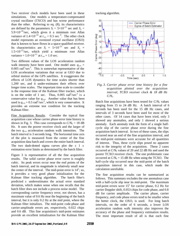
Fine Acquisition Results. Consider the typical fineacquisition case whose carrier phase error time history isshown in Fig. 3. This case corresponds to C/N0 = 18 dBHz. It uses the poorer receiver clock and the larger ofthe two qLOS acceleration random walk intensities. Thebatch interval is 3 seconds long. The horizontal time axisof the plot is measured from the center of the fineacquisition data batch and covers the entire batch interval.The two dash-dotted sigma curves plot the ± 1 σestimation error limits as determined by the batch filter.

Figure 3 is representative of all the fine acquisitionresults. The solid carrier phase error curve is roughlycubic. Its peak errors occur near the end points of thebatch interval, and its magnitude is relatively small nearthe center of the interval. The mid-point error is 14o; so,it provides a very good phase initialization for theKalman filter tracking algorithm. The batch filter'spredicted σ underestimates the actual error standarddeviation, which makes sense when one recalls that thebatch filter does not include a process noise model. Thecorresponding carrier frequency error, not shown, has amaximum value of 0.6 Hz near the beginning of the batchinterval, but it is only 0.2 Hz at the mid point, where theKalman filter initializes. The mid-point code-phase andcarrier-amplitude errors are, respectively, 0.022 chipsand 0.6 dB. This fine acquisition's mid-point estimatesprovide an excellent initialization for the Kalman filter

tracking algorithm.

Fig. 3. Carrier phase error time history for a fineacquisition plotted over the acquisitioninterval, TCXO receiver clock & 18 dB HzC/N0.

Batch fine acquisitions have been tested for C/N0 valuesranging from 15 to 24 dB Hz. A batch interval of 6seconds has been used for the 15 dB Hz cases, andintervals of 3 seconds have been used for most of theother cases. Of 14 cases that have been tried, only 3showed any anomalies, and only 1 showed a seriousanomaly. Each anomaly took the form of a single half-cycle slip of the carrier phase error during the fineacquisition batch interval. In two of these cases, the slipsoccurred near an end of the fine acquisition interval, andthe mid-point estimates were accurate for all quantitiesof interest. Thus, these cycle slips posed no apparentrisk to the integrity of the acquisition. These 2 casesoccurred at C/N0 values of 20 and 22 dB Hz and used thepoorer TCXO receiver clock. The one problematic caseoccurred at C/N0 = 15 dB Hz when using the TCXO. Thehalf-cycle slip occurred near the mid-point of the batchacquisition interval in this case, which made thecalculation unreliable.

The fine acquisition results can be summarized asfollows. This summary excludes the one anomalous casewith a half-cycle slip near its mid-point. The maximummid-point errors were 15o for carrier phase, 0.2 Hz forcarrier Doppler shift, 0.053 chips for code phase, and 0.8dB for carrier amplitude. The carrier phase, carrierfrequency, and code phase errors tend to be smaller whenthe better clock, the OXO, is used. For long batchintervals, on the order of 6 seconds, a lower LOSacceleration random walk intensity also improves theaccuracy of the phase and frequency estimation results.The most important result of all is that each fine

acquisition successfully initialized the Kalman filtertracker, as demonstrated by the fact that the trackermaintained lock for a significant interval following theinitialization.

Kalman Filter Tracking Results. The Kalman filter'sperformance is illustrated by the results of 2 typicalcases. Figure 4 presents the carrier phase error for thesetwo cases. Both cases use the poorer receiver clock, theTCXO, the high-dynamics assumption for the LOSacceleration random-walk intensity, and C/N0 = 18 dBHz. In fact, both cases track exactly the same RF front-end data. The only difference is that the top plotexplicitly considers data bit sign uncertainty only for thecurrent bit (Nb = 1), whereas the bottom plot explicitlyconsiders the 6 most recent data bit signs (Nb = 6). TheNb = 1 case maintains Doppler shift and code lock, but itexperiences numerous carrier cycle slips, 1 two-cycleslip, 2 one-cycle slips, and 3 half-cycle slips, all in just150 seconds of operation. The Nb = 6 case, on the otherhand, experiences just 1 half-cycle slip in 150 secondswith a few near slips as well. The Doppler shift errorsshow similar benefits from an increase in Nb. TheDoppler shift errors are 2.05 Hz max and 0.33 Hz RMSfor the Nb = 1 case, but they diminish to 1.11 Hz max and0.27 Hz RMS when Nb = 6. Thus, the explicitconsideration of more than 1 data bit sign makes thetracker more robust when operating on weak signals.

Fig. 4. EKF carrier phase tracking error timehistories for two cases, TCXO receiver clock& 18 dB Hz C/N0.

The Kalman filter's computed estimation error standarddeviation indicates when there are possible cycle slipproblems. The filter's standard deviation is derived byusing the xxmR~ square-root information matrix tocompute the estimation error covariance matrix. The

dotted curves on Fig. 4 are plus and minus plots of thefilter's computed carrier phase estimation error standarddeviation. These curves show spikes of about ¼ cycle atthe time of every cycle slip except for the last slip on thetop plot. On the bottom plot, the standard deviationcurves show periods with elevated uncertainty wheneverthe actual estimation error is experiencing some sort ofanomaly. Thus, the filter's statistical model of itsperformance is reasonable and informative, especiallywhen Nb is greater than 1.

The EKF tracking algorithm has been tried on a numberof cases. If the filter uses Nb = 1 bit and if the poorerTCXO receiver clock is used, then the EKF maintainsfull lock down to C/N0 = 22 dB Hz. Below this thresholdcycle slips start to crop up. The EKF maintains codelock and Doppler lock,. but with cycle slips, down toC/N0 = 18 dB Hz. At 15 dB Hz it eventually suffers atotal loss of lock. If Nb increases to 4, then the trackermaintains total lock down to C/N0 = 20 dB Hz. Thefrequency and average size of the cycle slips get reducedat 18 dB Hz when Nb = 4, but the EKF still suffers a totalloss of lock at 15 dB Hz. These results are summarizedin Fig. 5, which plots the tracker's RMS carrier phaseerror vs. the carrier-to-noise density, C/N0, when usingNb = 1 and the TCXO receiver clock. The dash-dottedcurve with the circle markers gives the filter's theoreticalcarrier phase error standard deviation, the dotted curvewith the square markers gives the actual RMS carrierphase errors, and the solid curve with the trianglemarkers gives the actual RMS carrier phase errors afterthe cycle slips have been artificially removed. Thisfigure shows that the system maintains full lock down to22 dB Hz and that its theoretical performance matchesits actual performance even down to 18 dB Hz oncecycle slips have been accounted for. An additional resultis plotted at C/N0 = 20 dB Hz for the case of Nb = 4.These points show that the filter maintains lock in thiscase and that the actual and theoretical performanceclosely match each other. The Nb = 1 tracker maintainslock to a threshold that is 3 dB Hz below the trackingthreshold for the PLL considered in Ref. 2, and the lockthreshold of the Nb = 4 tracker is 5 dB Hz below that ofRef. 2's PLL.

If the random dynamic variations of the carrier phase getreduced, then the situation improves markedly. If thebetter receiver clock, the OXO, gets used and if the LOSacceleration random walk intensity is reduced to amoderately conservative value for GEO, then the Nb = 1tracking algorithm maintains full lock with no carriercycle slips down to C/N0 = 15 dB Hz and possibly evenbelow that. This represents a significant performanceimprovement over the 23 dB Hz threshold for loss ofPLL lock given in Ref. 2 for the case of a perfectreceiver clock.

Fig. 5. EKF carrier phase tracking errorperformance as a function of C/N0, using Nb =1 and the TCXO.

Bit Errors, Sub-Frame Lock, and Autonomous Bit Aiding.When there are no cycle slips, the bit error rates forthese new tracking algorithms approach the theoreticalbit error rates that would exist with perfect carriertracking. For example, when C/N0 = 15 dB Hz a perfecttracker would experience a bit error rate of 13.0%. Thenew Kalman filter has a bit error rate of 14.1% whentracking a 15 dB Hz signal that has the benign phasedynamics of an OXO receiver clock and geosynchronousLOS accelerations.

Bit recognition becomes more problematic when cycleslips occur, but the decoded bits can be used to achievesub-frame lock even during times of significant cycleslips. Suppose that one correlates the known preamble,time-of-week (TOW), and 2nd-word parity bits of eachsub-frame with the tracker's decoded bits. Suppose, also,that one adds up these correlations over a number of sub-frames, but only after taking the absolute value of eachsub-frame's correlation in order to undo the effects ofpossible half-cycle slips. Then the resulting correlationfunction will have a peak when the known true bits arealigned correctly with the decoded bits. Figure 6 showsthe results of such a calculation. It corresponds to thesame case as the top plot on Fig. 4, the case with C/N0 =18 dB Hz, Nb = 1, and a TCXO. The absolute values ofthe correlations have been summed over 23 sub-frames.This correlation has an obvious peak at the correctcorrelation time, which means that sub-frame lock isachieved.

The ephemeris data bits can be determined in astraightforward manner when there are no cycle slips.This is done by voting the different values of the same bitthat get collected from different 30-second frames.Suppose that the bit error rate probability is perr and

suppose that the bit sign is to be decided by a simplemajority of the votes of its value from 2n+1 30-secondframes. Then the probability of getting the wrong resultfor any given ephemeris bit is

perrn = ∑−+

+−

=

−+n

j

jnerr

jerr

jnjnpp

0

)1(2

)!1(2!1)!(2)(1

(32)

Suppose that 2n+1 = 21 frames, which equals 630seconds of tracking data, and that the bit error rate is perr

= 0.14, as in the previously mentioned 15 dB Hz case.Then the probability that 21 votes will yield a majorityfor the wrong bit sign is perrn = 3.6×10-5, and theprobability that all of the bits in a 30-second frame willbe "elected" to the correct value is 0.95. Thus, 630seconds of data will be enough to correctly decode theephemeris in 19 out of 20 cases.

Fig. 6. Correlation of known sub-frame marker bitswith tracker's bit estimates, using Nb = 1, theTCXO, and C/N0 = 18 dB Hz, and summingabsolute values over 23 sub-frames.

The Kalman filter tracking algorithm lends itself topartial bit aiding. If one knows some of the bits, then onecan assign the values 1 or 0 to the a priori probabilities

)(+mp and )(−

mp . The sub-frame preamble, TOW, and2nd-word parity bits are known once sub-frame lock hasoccurred. In addition, many of the almanac bits and thehigh bits of the ephemeris data can be known ahead oftime because they do not change often. The details ofhow best to use such information remains to be workedout, but the current tracking system should provide ameans for exploiting it. The bottom plot of Fig. 4 showsthat the EKF is cognizant of the possibility of a half-cycle slip whenever one occurs if it uses Nb = 4. Thesign of the correlation with the sub-frame preamble, theTOW, and the 2nd-word parity bits could be used todetermine whether a half-cycle slip had occurred, andthat information could be used to go back and re-filterthe data in order to correct the cycle slips. Re-filtering

can be accomplished rapidly using stored values of the50 Hz I and Q accumulations along with the carrierNCO’s phase.

VI. SUMMARY AND CONCLUSIONS

Fine acquisition and tracking algorithms have beendeveloped for the carrier phase, the carrier amplitude andthe code phase of a weak GPS L1 C/A signal. The fineacquisition algorithm is needed in order to provide initialsignal phase and amplitude estimates with sufficientaccuracy to allow the extended Kalman filter trackingalgorithm to achieve lock. The fine acquisition startswith rough estimates of the carrier Doppler shift and thecode phase. It refines them by solving a sequence ofbatch maximum likelihood estimation problems that aredefined based on a time series of in-phase and quadratureaccumulations. It also estimates carrier phase and theinitial PRN code period of a navigation data bit. Thetracking algorithm implements a combined PLL/DLL byusing iterated extended Kalman filtering techniques.These techniques recursively optimize a fit between50 Hz I and Q accumulations and models of thesequantities that include sines and cosines of carrier phaseerrors and correlation functions evaluated at code phaseerrors. The Kalman filter includes a third-order carrierphase dynamic model that approximates the effects ofline-of-sight acceleration and receiver clock drift. Itscode phase dynamic model includes carrier aiding andrandom-walk code/carrier divergence. The Kalman filteruses a special Bayesian analysis of navigation data bitsigns that develops alternate signal state estimates fordifferent assumptions about a bit’s sign. It estimates aposteriori probabilities for each sign and uses theseprobabilities to mix the different state estimates into anoptimal reconstruction of the signal.

The fine acquisition algorithm and the EKF trackingalgorithm can successfully acquire and track very weakGPS signals. Signals with carrier-to-noise densities aslow as 22 dB Hz can be tracked with full carrier and codelock when the receiver clock is a temperaturecompensated crystal oscillator. Carrier cycle slipsdevelop as C/N0 drops below 22 dB Hz, and code andDoppler lock are lost at 15 dB Hz. There are severalavenues by which improvements can be made in thesethresholds. If the algorithm applies its Bayesian analysisto the 4 most recent data bits, then the full-lockthreshold decreases to 20 dB Hz. If the temperaturecompensated crystal oscillator is replaced by an ovenizedcrystal oscillator and if the dynamic motion of the uservehicle is benign, as is the case in geostationary Earthorbit, then full lock can be maintained at C/N0 = 15dB Hz.

ACKNOWLEDGMENTS

This work has been support in part by NASA GoddardSpace Flight Center through cooperative agreement no.NCC5-563 and by the NASA Office of Space Sciencethrough grant No. NAG5-12211. Luke Winternitz is themonitor for the cooperative agreement, and James Spannis the monitor for the grant.

REFERENCES1. Spilker, J.J. Jr., Digital Communications by Satellite,

Prentice-Hall, (Englewood Cliffs, N.J., 1977), pp. 336- 397,446-447, & 528-608.

2. Van Dierendonck, A.J., "GPS Receivers," in GlobalPositioning System: Theory and Applications, Vol. I,Parkinson, B.W. and Spilker, J.J. Jr., eds., American Instituteof Aeronautics and Astronautics, (Washington, 1996),pp. 329-407.

3. Moreau, M., Axelrad, P., Garrison, J.L., Kelbel, D., andLong, A., "GPS Receiver Architecture and ExpectedPerformance for Autonomous GPS Navigation in HighlyEccentric Orbits," Proc. of ION 55th Annual Meeting, June28-30, 1999, Cambridge, MA, pp. 653-665.

4. Long, A., Kelbel, D., Lee, T., Garrison, J., and Carpenter,J.R., "Autonomous Navigation Improvements for High-EarthOrbiters Using GPS," Paper no. MS00/13, Proc. of 15th

Intn’l. Symposium on Spaceflight Dynamics, CNES, June26-30, 2000, Biarritz, France, pp. unnumbered.

5. Moreau, M.C., Davis, E.P., Carpenter, J.R., Davis, G.W.,and Axelrad, P., “Results from the GPS Flight Experiment onthe High Earth Orbit AMSAT-OSCAR 40 Spacecraft,”Proc. of ION GPS , Sept. 24-27, 2002, Portland, OR.

6. Doherty, P.H., Delay, S.H., Valladares, C.E., and Klobuchar,J.A., "Ionospheric Scintillation Effects in the Equatorial andAuroral Regions," Proc. of ION GPS , Salt Lake City, UT,Sept. 19-22, 2000, pp. 662-671.

7. Psiaki, M.L., "Block Acquisition of Weak GPS Signals in aSoftware Receiver," Proc. of ION GPS , Salt Lake City, UT,Sept. 11-14, 2001, pp. 2838-2850.

8. Psiaki, M.L., "Smoother-Based GPS Signal Tracking in aSoftware Receiver," Proc. of ION GPS , Salt Lake City, UT,Sept. 11-14, 2001, pp. 2900-2913.

9. Brown, R.G. and Hwang, P.Y.C., Introduction to RandomSignals and Applied Kalman Filtering, 3rd Edition, J.Wiley & Sons, (New York, 1997), pp. 428-432.

10. Gill, P.E., Murray, W., and Wright, M.H., PracticalOptimization, Academic Press, (New York, 1981), pp. 88-93, 99-114, & 133-140.

11. Bierman, G.J., Factorization Methods for DiscreteSequential Estimation, Academic Press, (New York, 1977),pp. 69-76, 115-122.

12. Psiaki, M.L., Theiler, J., Bloch, J., Ryan, S., Dill, R.W., andWarner, R.E., “ALEXIS Spacecraft Attitude Reconstructionwith Thermal/Flexible Motions Due to Launch Damage,”Journal of Guidance, Control, and Dynamics, Vol. 20(5),1997, pp. 1033-1041.