Embed Size (px)
Citation preview
Government Spending Multipliers and Recessions
October 2010
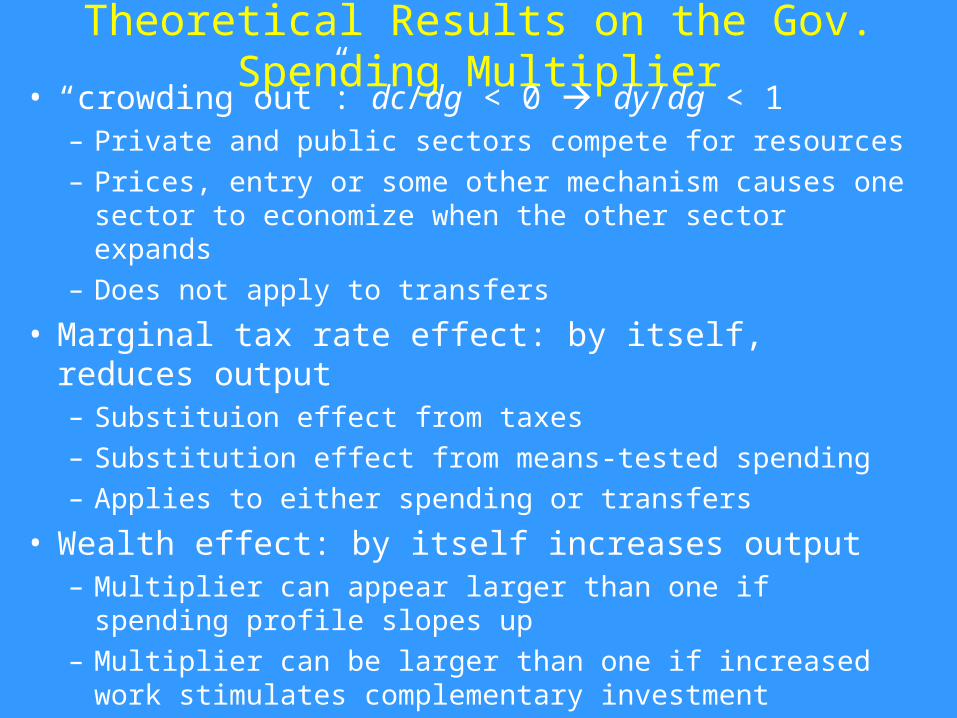
Theoretical Results on the Gov. Spending Multiplier• “crowding out”: dc/dg < 0 dy/dg < 1
– Private and public sectors compete for resources
– Prices, entry or some other mechanism causes one sector to economize when the other sector expands
– Does not apply to transfers
• Marginal tax rate effect: by itself, reduces output– Substituion effect from taxes
– Substitution effect from means-tested spending
– Applies to either spending or transfers
• Wealth effect: by itself increases output– Multiplier can appear larger than one if spending profile slopes
up
– Multiplier can be larger than one if increased work stimulates complementary investment
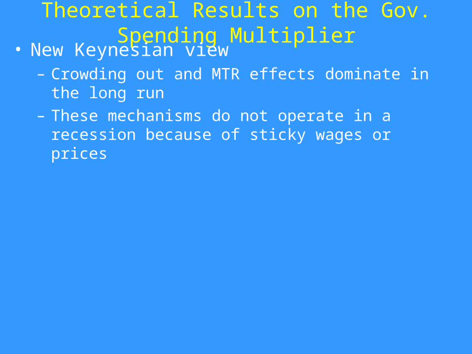
Theoretical Results on the Gov. Spending Multiplier• New Keynesian view
– Crowding out and MTR effects dominate in the long run
– These mechanisms do not operate in a recession because of sticky wages or prices
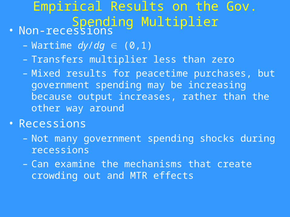
Empirical Results on the Gov. Spending Multiplier• Non-recessions
– Wartime dy/dg (0,1)
– Transfers multiplier less than zero
– Mixed results for peacetime purchases, but government spending may be increasing because output increases, rather than the other way around
• Recessions– Not many government spending shocks during recessions
– Can examine the mechanisms that create crowding out and MTR effects
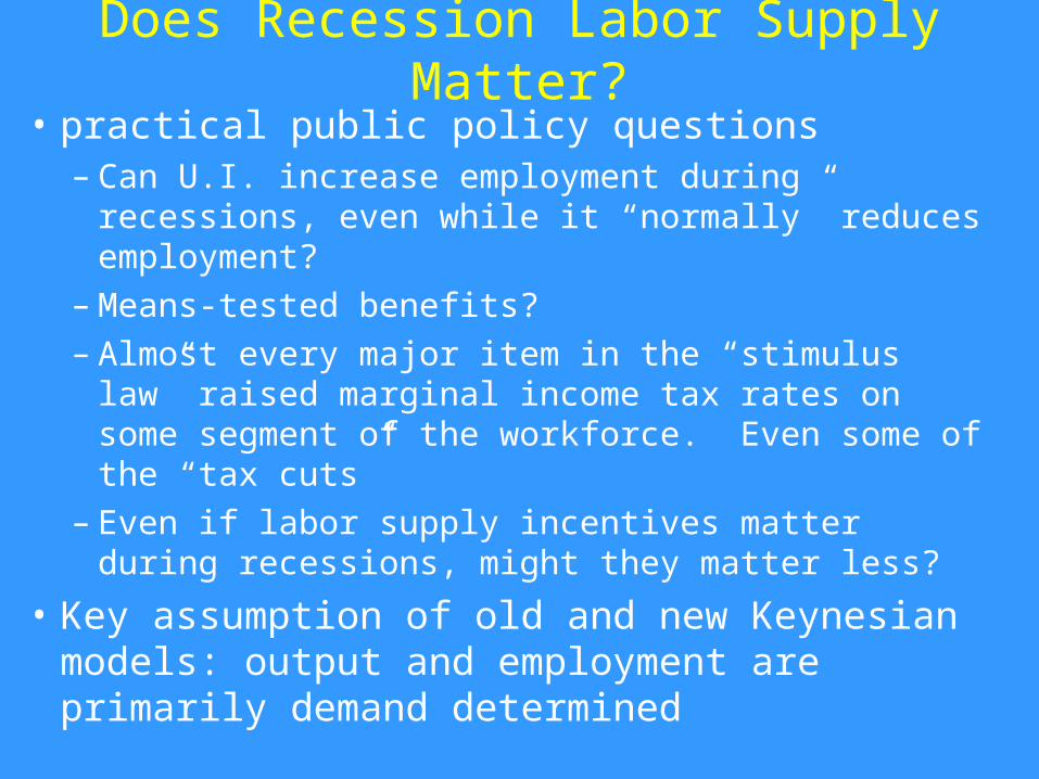
Does Recession Labor Supply Matter?
• practical public policy questions– Can U.I. increase employment during recessions, even
while it “normally” reduces employment?– Means-tested benefits?– Almost every major item in the “stimulus law” raised
marginal income tax rates on some segment of the workforce. Even some of the “tax cuts”
– Even if labor supply incentives matter during recessions, might they matter less?
• Key assumption of old and new Keynesian models: output and employment are primarily demand determined
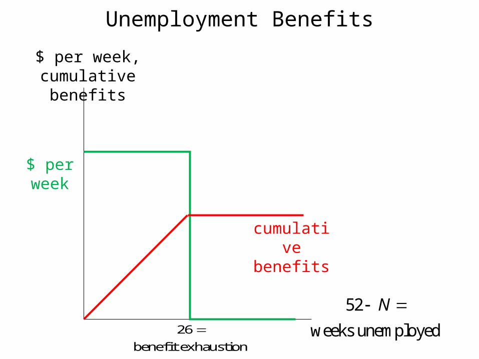
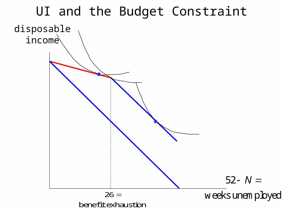
52
weeks unemployed
N
Unemployment Benefits
26
benefit exhaustion
$ per week, cumulative benefits
$ per week
cumulative benefits
52
weeks unemployed
N
UI and the Budget Constraintdisposable
income
26
benefit exhaustion
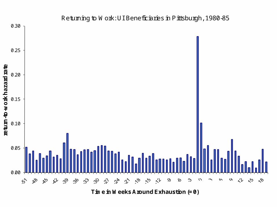
0.00
0.05
0.10
0.15
0.20
0.25
0.30
retu
rn-t
o-w
ork
ha
zard
rate
Time in Weeks Around Exhaustion (= 0)
Returning to Work: UI Beneficiaries in Pittsburgh, 1980-85
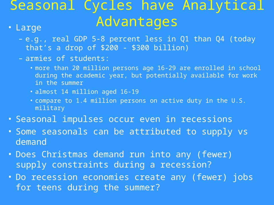
Seasonal Cycles have Analytical Advantages• Large
– e.g., real GDP 5-8 percent less in Q1 than Q4 (today that’s a drop of $200 - $300 billion)
– armies of students:• more than 20 million persons age 16-29 are enrolled in school during
the academic year, but potentially available for work in the summer
• almost 14 million aged 16-19
• compare to 1.4 million persons on active duty in the U.S. military
• Seasonal impulses occur even in recessions• Some seasonals can be attributed to supply vs demand• Does Christmas demand run into any (fewer) supply
constraints during a recession?• Do recession economies create any (fewer) jobs for teens
during the summer?

N
labor supply
labor demand
Wage Floor & Job Shortage
*N
$ per hour
Y “Unemployed” = would accept a job paying the going wage
N
/Y P
*N
*Y
P
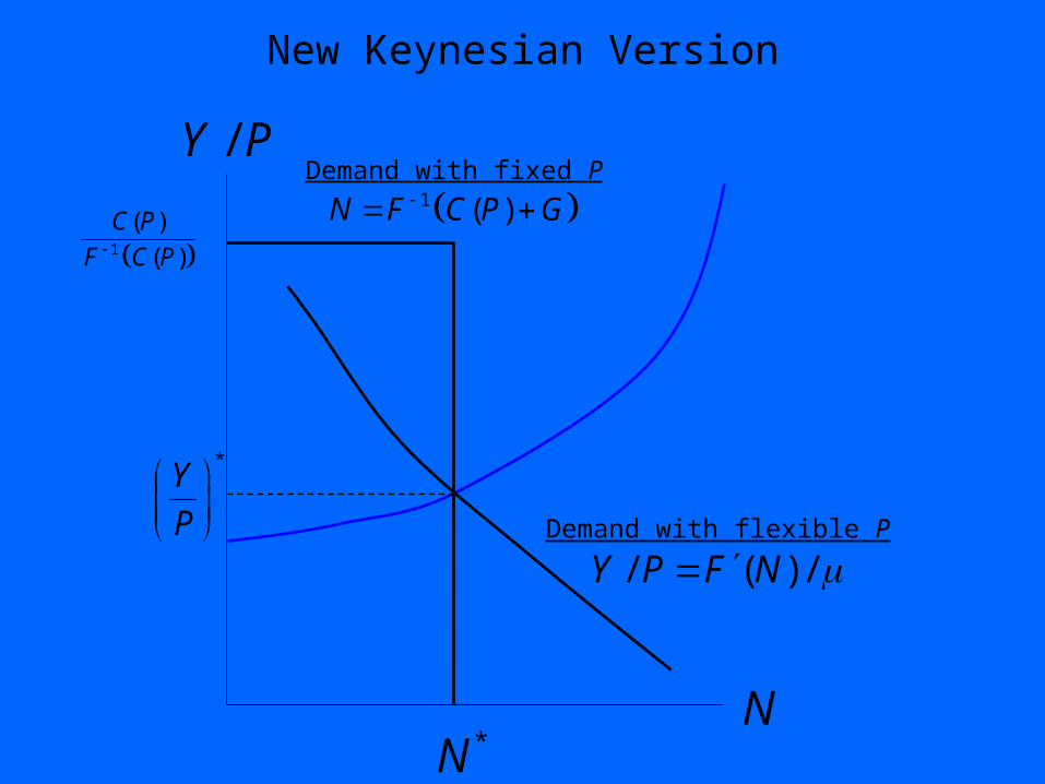
New Keynesian Version
/ ( ) /Y P F N Demand with flexible P
1 ( )N F C P G Demand with fixed P
1
( )
( )
C P
F C P

Non-Wage Mechanisms• Search• Monopoly labor union: could “over-shift” supply
– i.e., if recessions are times when monopoly union power is especially important, then employment could be more sensitive to supply during a recession
• Job characteristics model unemployment can exist even while labor supply
matters at the margin, perhaps even more than it would without unemployment
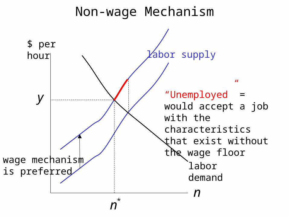
n
labor supply
labor demand
Non-wage Mechanism
*n
$ per hour
y
wage mechanism is preferred
“Unemployed” = would accept a job with the characteristics that exist without the wage floor
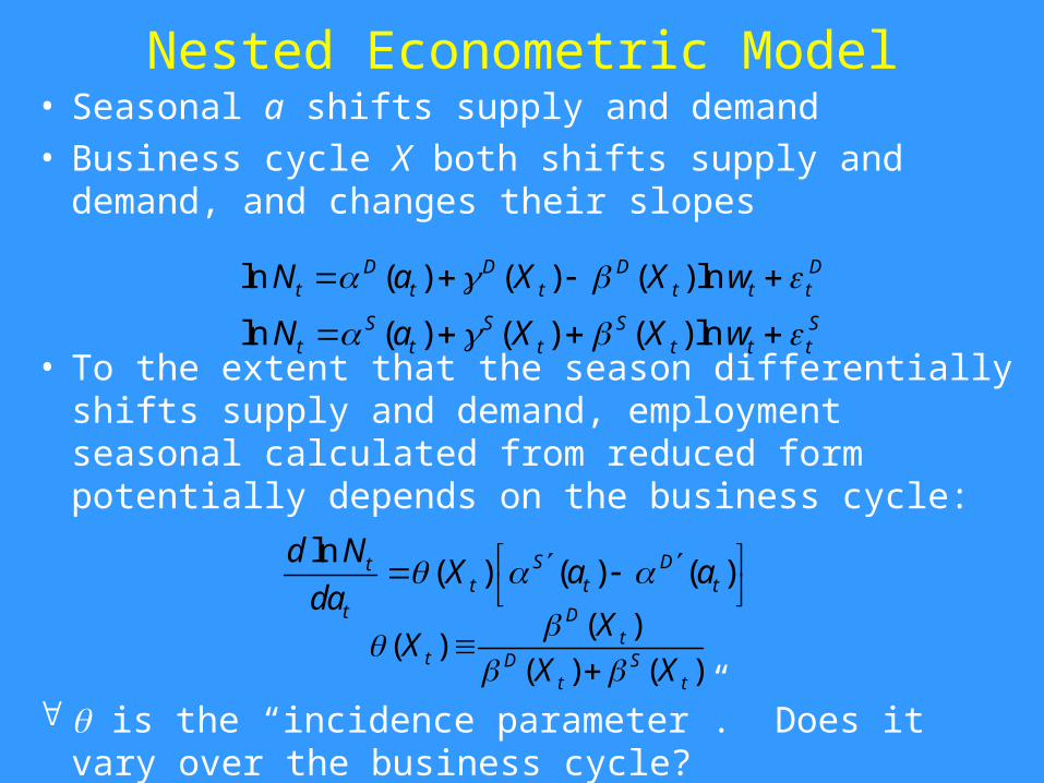
Nested Econometric Model• Seasonal a shifts supply and demand• Business cycle X both shifts supply and demand, and
changes their slopes
• To the extent that the season differentially shifts supply and demand, employment seasonal calculated from reduced form potentially depends on the business cycle:
is the “incidence parameter”. Does it vary over the business cycle?
ln ( ) ( ) ( ) lnD D D Dt t t t t tN a X X w
ln ( ) ( ) ( ) lnS S S St t t t t tN a X X w
ln( ) ( ) ( )S Dt
t t tt
d NX a a
da
( )
( )( ) ( )
Dt
t D St t
XX
X X

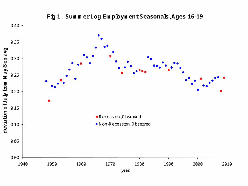
Seasonally Unadjusted Data• Household Survey: Monthly employment by age group• Establishment survey: Monthly employment by industry• Monthly Retail Sales• Summer seasonal
– deviation of log July value from May-Sep average
– May-Sep average is weighted in years when the Census Bureau reference week in July is not equidistant from May and September reference weeks. (these weights have almost no effect on the results)
• Christmas seasonal– deviation of log Nov-Dec value from Oct-Jan average
– also December only version
– similar results if Jan-Feb is compared to Dec-May interpolation
0.00
0.05
0.10
0.15
0.20
0.25
0.30
0.35
0.40
1940 1950 1960 1970 1980 1990 2000 2010
de
via
tio
n o
f Ju
ly fr
om
Ma
y-S
ep
avg
year
Fig 1. Summer Log Employment Seasonals, Ages 16-19
Recession, Observed
Non-Recession, Observed

0.00
0.05
0.10
0.15
0.20
0.25
0.30
0.35
0.40
1940 1950 1960 1970 1980 1990 2000 2010
de
via
tio
n o
f Ju
ly fr
om
Ma
y-S
ep
avg
year
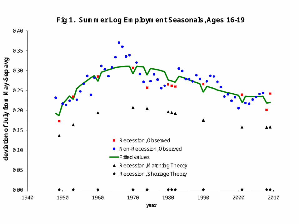
Fig 1. Summer Log Employment Seasonals, Ages 16-19
Recession, Observed
Non-Recession, Observed
Fitted values
0.00
0.05
0.10
0.15
0.20
0.25
0.30
0.35
0.40
1940 1950 1960 1970 1980 1990 2000 2010
de
via
tio
n o
f Ju
ly fr
om
Ma
y-S
ep
avg
year
Fig 1. Summer Log Employment Seasonals, Ages 16-19
Recession, Observed
Non-Recession, Observed
Fitted values
Recession, Matching Theory
Recession, Shortage Theory

Table 1. Summer Seasonals For Employment and Unemployment, by Age Group
Statistic 16-17 18-19 16-19 20-24 25-34 16+Emp. 38.2 23.6 29.6 6.0 -1.3 2.0
Non-recession Seasonal, (0.6) (0.5) (0.5) (0.2) (0.1) (0.1)100ths of log points Unemp. 38.9 19.0 28.5 6.7 4.4 10.2
(2.3) (1.9) (1.8) (1.1) (1.2) (0.8)
Emp. -1.92 -1.67 -1.82 -0.02 -0.05 0.02Recession Coefficient, (1.05) (0.78) (0.75) (0.34) (0.15) (0.16)100ths of log points Unemp. -3.47 1.44 -1.28 -2.05 1.08 -0.71
(3.81) (3.09) (2.89) (1.82) (1.94) (1.34)
Emp. 0.95 0.93 0.94 1.00 1.04 1.01Recession Seasonal/ (0.03) (0.03) (0.02) (0.06) (0.12) (0.08)Non-recession Seasonal Unemp. 0.91 1.08 0.96 0.69 1.25 0.93
(0.10) (0.16) (0.10) (0.26) (0.46) (0.13)
Notes: OLS standard errors in parentheses
Age Group
Each column of the Table reports results from an employment regression and an unemployment regression. The dependent variable is 100 times the July deviation of log per capita employment (unemployment) from the average of May and September.
Independent variables are: NBER recession dummy, a 3rd order time polynomial (time 0 = 1980) and a constant.When applicable, the May-September average is weighted to reflect that the July reference week is not equidistant between the May and September reference weeks
0.00
0.10
0.20
0.30
0.40
0.50
0.60
0.70
0.80
1940 1950 1960 1970 1980 1990 2000 2010
de
via
tio
n o
f Ju
ly fr
om
Ma
y-S
ep
avg
year
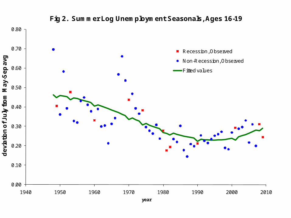
Fig 2. Summer Log Unemployment Seasonals, Ages 16-19
Recession, Observed
Non-Recession, Observed
Fitted values
Reasons to Think Summer Supply Shift Exceeds Demand
• Sheer numbers– 20+ million students aged 16-29 released from school
– What possibly could be a summer demand shift of that size? Even doubling the size of the military would be smaller
• If demand shifted so much:– why are summer unemployment rates above normal for all age
groups?
– why isn’t summer employment high for ages 25+?
– why aren’t Q3 teen weekly wages higher than in other quarters?
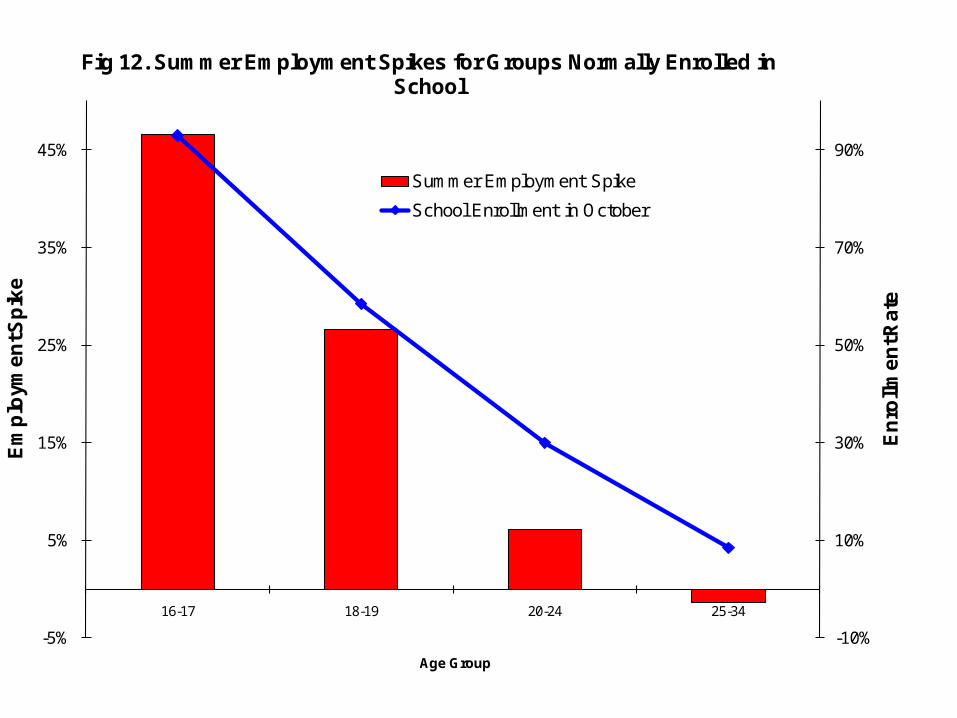
– why does the summer employment seasonal mimic the school enrollment pattern?
Statistic Nov-Dec Dec onlyRetail Sales 16.00 26.40
(0.59) (0.78)Emp., Est. 1.20 1.60
Non-recession Seasonal, (0.04) (0.05)100ths of log points Emp., HH 0.70 1.00
(0.05) (0.07)Unemp. -6.60 -10.00
(0.59) (0.71)Labor Force 0.30 0.40
(0.05) (0.07)
Retail Sales -1.32 -2.00(0.88) (1.18)
Emp., Est. -0.08 -0.14Recession Coefficient, (0.06) (0.08)100ths of log points Emp., HH 0.06 0.02
(0.09) (0.11)Unemp. -1.90 -0.84
(1.02) (1.23)Labor Force -0.06 -0.09
(0.08) (0.11)
Retail Sales 0.92 0.92(0.05) (0.04)
Emp., Est. 0.93 0.91Recession Seasonal/ (0.05) (0.05)Non-recession Seasonal Emp., HH 1.03 1.02
(0.10) (0.10)Unemp. 1.29 1.08
(0.19) (0.14)Labor Force 0.79 0.79
(0.21) (0.28)
Notes: OLS standard errors in parentheses
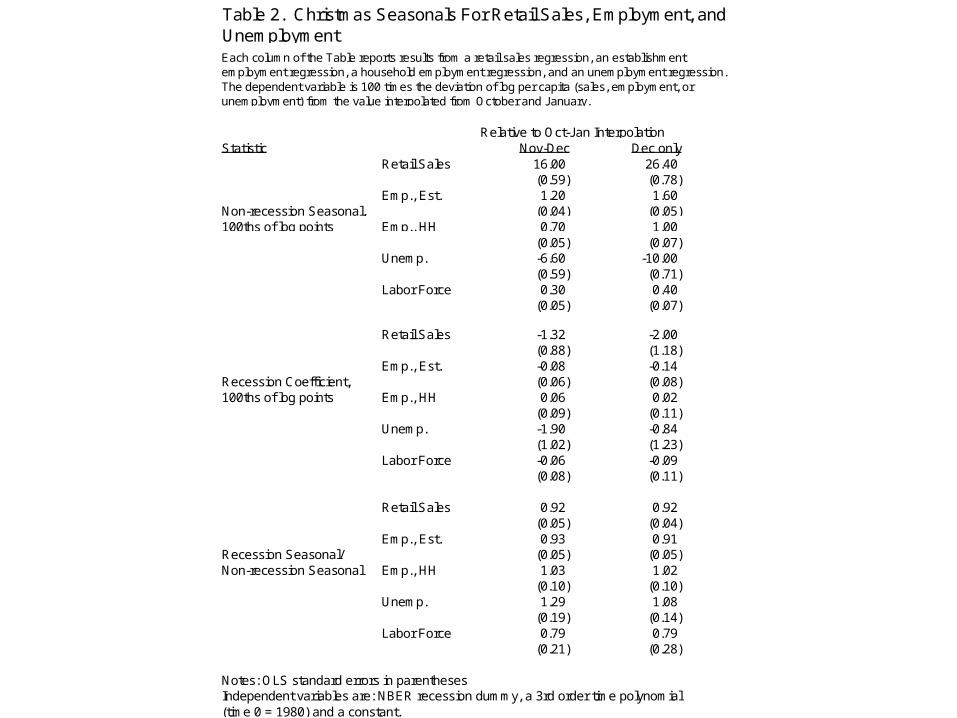
Table 2. Christmas Seasonals For Retail Sales, Employment, and Unemployment
Relative to Oct-Jan Interpolation
Independent variables are: NBER recession dummy, a 3rd order time polynomial (time 0 = 1980) and a constant.
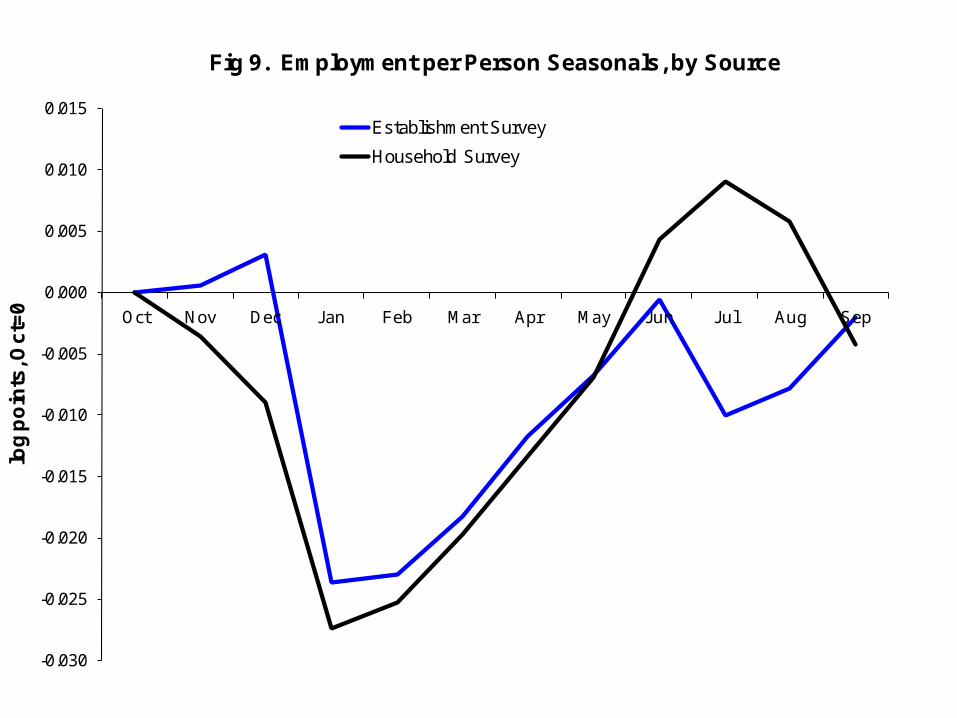
Each column of the Table reports results from a retail sales regression, an establishment employment regression, a household employment regression, and an unemployment regression. The dependent variable is 100 times the deviation of log per capita (sales, employment, or unemployment) from the value interpolated from October and January.

Fig 3. Christmas Log Payroll Employment Seasonals, All Ages
0.000
0.005
0.010
0.015
0.020
0.025
0.030
0.035
0.040
0.045
1940 1950 1960 1970 1980 1990 2000 2010
year
de
via
tio
n o
f N
ov
-De
c f
rom
Oc
t-J
an
av
g
Recession, Observed
Non-Recession, Observed
Fitted values
Recession, Matching Theory
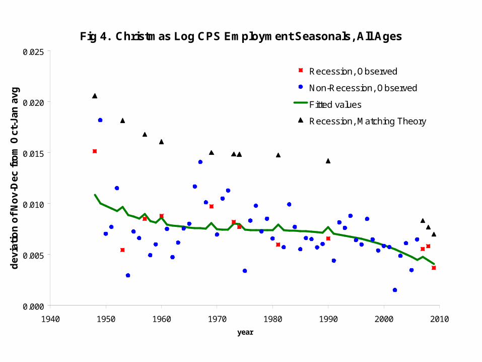
Fig 4. Christmas Log CPS Employment Seasonals, All Ages
0.000
0.005
0.010
0.015
0.020
0.025
1940 1950 1960 1970 1980 1990 2000 2010
year
de
via
tio
n o
f N
ov
-De
c f
rom
Oc
t-J
an
av
g
Recession, Observed
Non-Recession, Observed
Fitted values
Recession, Matching Theory
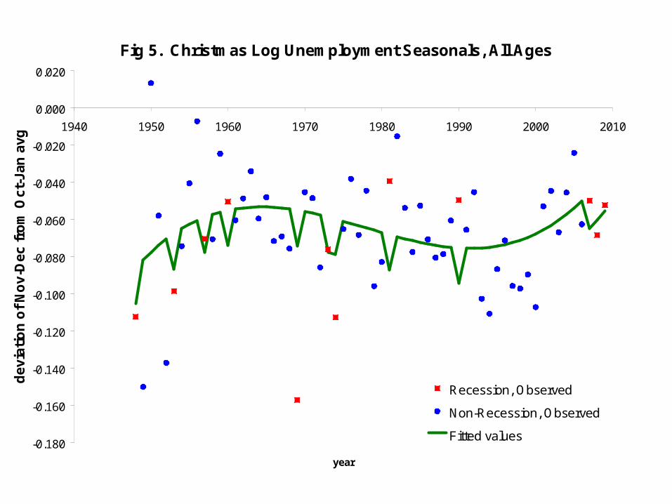
Fig 5. Christmas Log Unemployment Seasonals, All Ages
-0.180
-0.160
-0.140
-0.120
-0.100
-0.080
-0.060
-0.040
-0.020
0.000
0.020
1940 1950 1960 1970 1980 1990 2000 2010
year
de
via
tio
n o
f N
ov
-De
c f
rom
Oc
t-J
an
av
g
Recession, Observed
Non-Recession, Observed
Fitted values
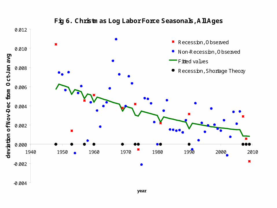
Fig 6. Christmas Log Labor Force Seasonals, All Ages
-0.004
-0.002
0.000
0.002
0.004
0.006
0.008
0.010
0.012
1940 1950 1960 1970 1980 1990 2000 2010
year
de
via
tio
n o
f N
ov
-De
c f
rom
Oc
t-J
an
av
g
Recession, Observed
Non-Recession, Observed
Fitted values
Recession, Shortage Theory
-0.15
-0.10
-0.05
0.00
0.05
0.10
0.15
0.20
0.25
0.30
Oct Nov Dec Jan Feb Mar Apr May Jun Jul Aug Sep
log
po
ints
, Oc
t=0
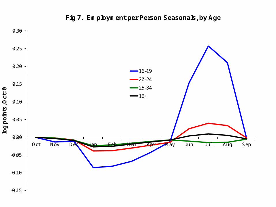
Fig 7. Employment per Person Seasonals, by Age
16-19
20-24
25-34
16+
-0.10
0.00
0.10
0.20
0.30
0.40
0.50
0.60
Oct Nov Dec Jan Feb Mar Apr May Jun Jul Aug Sep
log
po
ints
, Oc
t=0
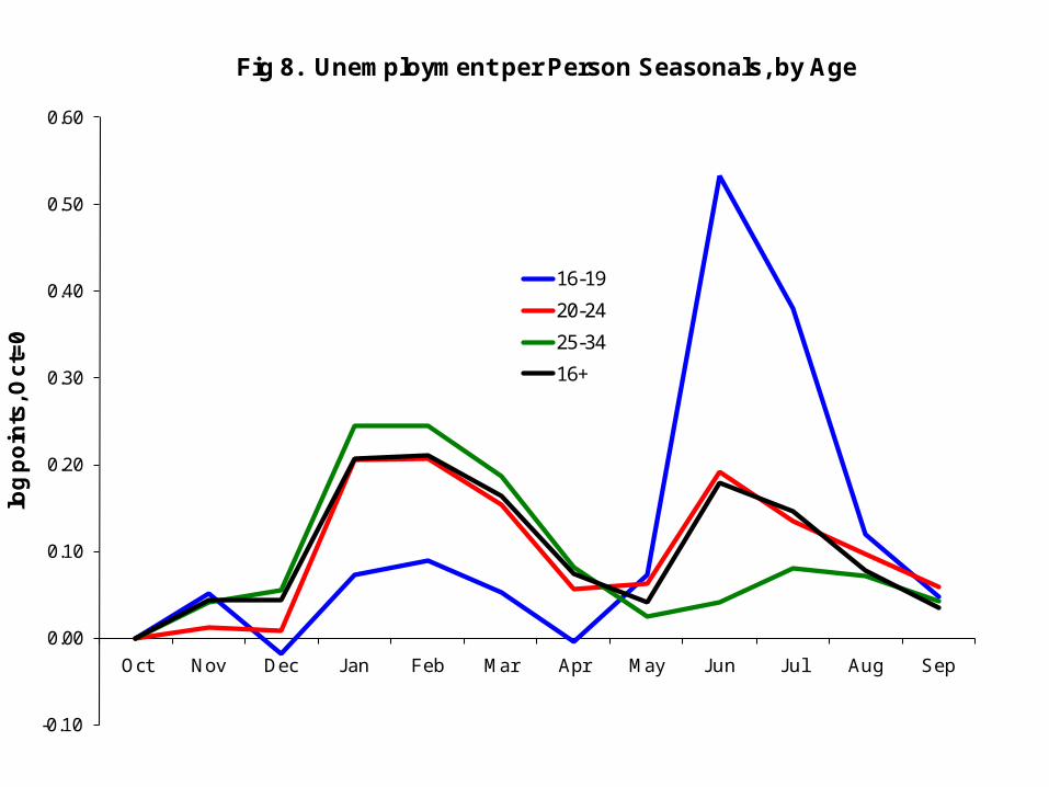
Fig 8. Unemployment per Person Seasonals, by Age
16-19
20-24
25-34
16+
-0.030
-0.025
-0.020
-0.015
-0.010
-0.005
0.000
0.005
0.010
0.015
Oct Nov Dec Jan Feb Mar Apr May Jun Jul Aug Sep
log
po
ints
, Oc
t=0
Fig 9. Employment per Person Seasonals, by Source
Establishment Survey
Household Survey
-0.150
-0.100
-0.050
0.000
0.050
0.100
0.150
0.200
Oct Nov Dec Jan Feb Mar Apr May Jun Jul Aug Seplog
po
ints
, Oc
t=0
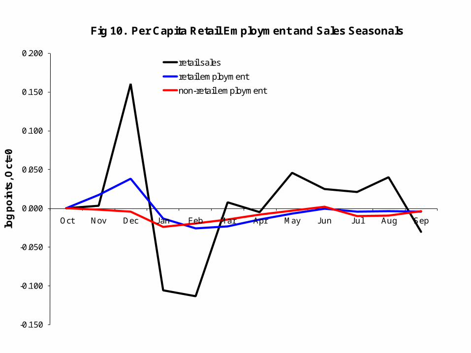
Fig 10. Per Capita Retail Employment and Sales Seasonals
retail sales
retail employment
non-retail employment
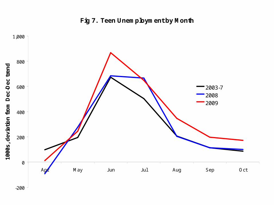
Fig 7. Teen Unemployment by Month
-200
0
200
400
600
800
1,000
Apr May Jun Jul Aug Sep Oct
10
00
s,
de
via
tio
n f
rom
De
c-D
ec
tre
nd
2003-720082009
-10%
10%
30%
50%
70%
90%
-5%
5%
15%
25%
35%
45%
16-17 18-19 20-24 25-34
En
rollm
en
t Ra
te
Em
plo
yme
nt S
pik
e
Age Group
Fig 12. Summer Employment Spikes for Groups Normally Enrolled in School
Summer Employment Spike
School Enrollment in October
-10%
10%
30%
50%
70%
90%
-5%
5%
15%
25%
35%
45%
16-17 18-19 20-24 25-34
En
rollm
en
t Ra
te
Un
em
plo
ymen
t Sp
ike
Age Group
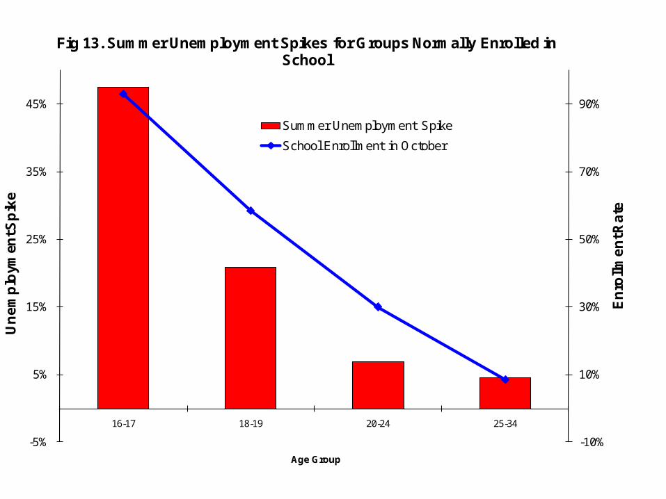
Fig 13. Summer Unemployment Spikes for Groups Normally Enrolled in School
Summer Unemployment Spike
School Enrollment in October
Conclusions• Economic theory does not tell us whether labor supply
would matter more or less during a recession.• Economic theory does not tell us whether labor demand
would matter more or less during a recession.• the summer and Christmas seasonals for employment
and unemployment are essentially the same number of log points in recession years and non-recession years
• Even in 2008 and 2009• Results contradict old- and new-Keynesian models• Results are consistent with the view that labor markets
are especially “distorted” during recessions