Government Spending Multipliers in Good Times

and in Bad: Evidence from U.S. Historical Data

Valerie A. Ramey

University of California, San Diego and NBER

Sarah Zubairy

Texas A&M University

Abstract

We investigate whether U.S. government spending multipliers are higher during periods

of economic slack or when interest rates are near the zero lower bound. Using new

quarterly historical U.S. data covering multiple large wars and deep recessions, we esti-

mate multipliers that are below unity irrespective of the amount of slack in the economy.

These results are robust to two leading identification schemes, two different estimation

methodologies, and many alternative specifications. In contrast, the results are more

mixed for the zero lower bound state, with a few specifications implying multipliers as

high as 1.5.

We are grateful to Harald Uhlig, Roy Allen, Alan Auerbach, Graham Elliott, Yuriy Gorodnichenko, Jim Hamil-ton, Òscar Jordà, Michael Owyang, Carolin Pflueger, Garey Ramey, Tatevik Sekhposyan, Mark Watson, Jo-hannes Wieland, anonymous referees, and participants at many conferences and seminars for very helpfulsuggestions. We thank Michelle Ramey for excellent research assistance.

1 Introduction

What is the multiplier on government spending? The policy debates that started during the

Great Recession have led to an outpouring of research on this question. Most studies have

found estimates of modest multipliers in aggregate data, often below unity. If multipliers are

indeed this low, they suggest that increases in government purchases do not stimulate private

activity and that fiscal consolidations based on reducing government purchases are unlikely

to do much harm to the private sector.

Most of the estimates are based on averages for a particular country over a particular his-

torical period. Because there is no scope for controlled, randomized trials on countries, all

estimates of aggregate government multipliers are necessarily dependent on historical hap-

penstance. Theory tells us that details such as the persistence of spending changes, how they

are financed, how monetary policy reacts, and the tightness of the labor market can signifi-

cantly affect the magnitude of the multipliers. Unfortunately, the data do not present us with

clean natural experiments that can answer these questions. While the recent U.S. stimulus

package was purely deficit financed and undertaken during a period of high unemployment

and accommodative monetary policy, it was enacted in response to a weak economy and

hence any aggregate estimates are subject to simultaneous equations bias.

During the last several years, the literature has begun to explore whether estimates of

government spending multipliers vary depending on circumstances. One strand of this lit-

erature considers the possibility that multipliers are higher than normal during recessions

(e.g. Barro and Redlick (2011), Auerbach and Gorodnichenko (2012, 2013), Fazzari et al.

(2015)). Another strand of the literature considers how monetary policy affects government

spending multipliers. New Keynesian DSGE models show that when interest rates are stuck

at the zero lower bound, multipliers can be higher than in normal times (e.g. Cogan et al.

(2010), Christiano et al. (2011), Coenen and et al. (2012)).

2

This paper contributes to the empirical literature by conducting a comprehensive inves-

tigation of whether government spending multipliers in the U.S. differ according to two po-

tentially important features of the economy: (1) the amount of slack in the economy and (2)

whether interest rates are near the zero lower bound. We show that the post-WWII U.S. data

does not contain enough information to distinguish multipliers across either of these states

at most horizons. Extending the initial analysis in Owyang et al. (2013), we exploit the fact

that the entire 20th Century contains potentially richer information than the post-WWII data

that has been the focus of most of the recent research. We create a new quarterly data set

for the U.S. extending back to 1889. This sample includes episodes of huge variations in

government spending, wide fluctuations in unemployment, prolonged periods near the zero

lower bound of interest rates, and a variety of tax responses.

This paper extends the small, but growing, literature on state dependence of government

spending multipliers in two additional ways. First, our paper analyzes state-dependence

involving the important zero lower bound state. Only two previous papers specifically esti-

mated multipliers over an episode of the zero lower bound, Ramey (2011) for the U.S. and

Crafts and Mills (2013) for the U.K., but neither tested for differences relative to normal

times. Second, our paper contributes to the general state-dependent multiplier literature by

highlighting some key methodological issues that arise. In particular, we show that some

of the most widely-cited findings of high multipliers during recessions are due to assump-

tions that may be at odds with the data generating process. We show that the finding of

high multipliers during low growth periods disappears when data-consistent assumptions are

used.

Using Jordà’s (2005) local projection method we find no evidence that government spend-

ing multipliers are high during high unemployment states. Most estimates of the multiplier

are between 0.3 and 0.8. We find a statistically significant difference in multipliers across

states only when we identify spending shocks following Blanchard and Perotti’s (2002)

3

method; however, the difference is due not to high multipliers in the high unemployment

state but to very low multipliers in the low unemployment state. We perform extensive ro-

bustness checks with respect to our measures of state, sample period, the behavior of taxes,

and alternative estimation frameworks and find little change in the estimates.

We find mixed evidence on the size of the multiplier at the zero lower bound. For the full

sample, there is no evidence of multipliers greater than one at the zero lower bound. When

we exclude the rationing periods of WWII, however, we find multipliers as high as 1.5 in the

zero lower bound state in some cases.

We also demonstrate that most of the differences in conclusions between our work and

that of the leading alternative study on state-dependent multipliers of Auerbach and Gorod-

nichenko (2012) lie in subtle, yet crucial, assumptions underlying the construction of impulse

response functions on which the multipliers are based. In contrast to linear models, where

the calculation of impulse response functions is a straightforward undertaking, constructing

impulse response functions in nonlinear models is fraught with complications. Furthermore,

when we apply their threshold VAR method to our longer sample, but in a way that is more

consistent with the data-generating process, we find results that are very similar to those

produced by the Jordà method.

The paper proceeds as follows. We begin by discussing the motivation for using a his-

torical sample and then conduct some case studies of wars in Section 2. In Section 3 we

introduce the econometric methodology. In Section 4, we present our measures of slack and

then present estimates of a model in which multipliers are allowed to vary according to the

amount of slack in the economy. We also conduct various robustness checks. Section 5

tests theories that predict that multipliers should be greater when interest rates are at the zero

lower bound. Section 6 explores alternative methodologies and explains why our results are

different from the pre-existing estimates in the literature and the final section concludes.

4

2 Historical Sample and Case Studies

In this section, we begin by motivating why we construct a new historical data set to study

multipliers. We then briefly describe the data construction, leaving most details to the data

appendix. Finally, because there are three wars in our sample that potentially play an influ-

ential role for our estimates, we conduct brief case studies of those three periods.

2.1 Why Use Historical Data?

The ideal way to measure the effects of government purchases on an economy would be

to ask the IMF to conduct a randomized control trial across countries, randomly assigning

changes in government spending (and how they are financed) across countries and then using

simple statistical techniques to estimate the effects. Obviously, such an experiment is impos-

sible. Thus, macroeconomists must resort to estimating multipliers by exploiting "natural

experiments" or other identification methods using time series on national historical data.1

To be informative, the identified changes in government spending must be exogenous and big

enough to be able to extract their effects from the many other economic shocks hitting the

economy. The challenge becomes even greater once one attempts to estimate state-dependent

multipliers since informative estimates require that the states span a sufficient portion of the

sample and that the exogenous changes in government spending be spread across the states.

Long samples of historical data for the U.S. meet this challenge well since U.S. histori-

cal data includes many more periods of slack, one more extended period near the zero lower

bound, and much larger variations in government spending during world wars. Historical

samples come with their own potential problems, though. For example, one may wonder

1. The natural experiments ideally involve aggregate data. As Nakamura and Steinsson (2014) and Farhiand Werning (2016) show, the multipliers estimated from natural experiments that involve cross-state or cross-province differences are not the same as aggregate multipliers. A number of cross-state analyses find someevidence of higher multipliers when the state unemployment rate is higher, but translating those to aggregatemultipliers is not straightforward.

5

whether the U.S. economy has changed so much over time that estimates from historical

samples are uninformative for modern policy. We would argue that, if anything, the changes

over time would reduce multipliers in recent years. The models that produce some of the

highest multipliers are ones in which a higher fraction of consumers are rule-of-thumb or

hand-to-mouth consumers. Increases over time in financial market access and consumer so-

phistication should reduce the fraction of rule-of-thumb consumers, thus reducing multipliers

in recent years. Separately, monetary policy and fiscal policy have been conducted differ-

ently over various periods, but both the pre-WWII and post-WWII sample display periods

of more or less monetary accommodation and more or less deficit financing of government

spending. Thus, we believe that estimates from historical samples can be informative for

modern policy debates.

Alternatively, one might argue that since wars are "abnormal," we should exclude them.

Friedman (1952) countered this argument years ago:

The widespread tendency in empirical studies of economic behavior to discard

war years as "abnormal," while doubtless often justified, is, on the whole, unfor-

tunate. The major defect of the data on which economists must rely - data gen-

erated by experience rather than deliberately contrived experiment - is the small

range of variation they encompass. Experience in general proceeds smoothly

and continuously. In consequence, it is difficult to disentangle systematic effects

from random variation since both are of much the same order of magnitude.

From this point of view, data for wartime periods are peculiarly valuable. At

such times, violent changes in major economic magnitudes occur over relatively

brief periods, thereby providing precisely the kind of evidence that we would

like (to) get by "critical" experiments if we could conduct them. Of course,

the source of the changes means that the effects in which we are interested are

necessarily intertwined with others that we would eliminate from a contrived

6

experiment. But this difficulty applies to all our data, not to data for wartime

periods alone.

We also believe that there is much to be learned from war-time periods, but do recognize

the potential effects of confounding factors. We will discuss those factors in the case studies

below and in the sample exclusions in the econometric estimation.

A separate issue is whether the economy responds to military spending in the same way

it would respond to other types of government purchases, e.g. non-defense consumption,

infrastructure, etc. This is a valid concern and is related to the standard question of whether

a local average treatment effect (LATE) is equal to the average treatment effect (ATE). Our

baseline instrument will be an updated version of Ramey’s (2011) military news variable, so

it only captures news about changes in military spending and most of actual spending arrives

with delay. In order to broaden our range of treatments, we will also use the Blanchard and

Perotti (2002) shock. This identification scheme is based on the assumption that within-

quarter government spending does not contemporaneously respond to macroeconomic vari-

ables. While in response to a military news shock, government spending rises with a delay,

the Blanchard-Perotti shocks also help capture the effects of a shock where spending peaks

close to impact. Using the Blanchard-Perotti shock involves a tradeoff, however, since this

type of shock is both more sensitive to potential measurement errors in the historical data

and subject to the critique that it is likely to have been anticipated.

2.2 Data Description

In order to exploit the information in the historical sample, we construct quarterly data from

1889 through 2015 for the U.S. We choose to estimate our model using quarterly data rather

than annual data because agents often react quickly to news about government spending and

7

the state of the economy can change abruptly.2 The historical series include real GDP, the

GDP deflator, government purchases, federal government receipts, population, the unem-

ployment rate, interest rates, and defense news.

The data appendix contains full details, but we highlight some of the features of the data

here. From 1939 to the present, we use available published quarterly series. For the earlier

periods, we follow Gordon and Krenn (2010) by using various higher frequency series to

interpolate existing annual series.3 In most cases, we use the proportional Denton procedure

which results in series that average up to the annual series.

The annual real GDP data combine the series from Historical Statistics of the U.S. (Carter

et al. (2006)) for 1889 through 1928 and the NIPA data from 1929 to the present. The annual

data are interpolated with Balke and Gordon’s (1986) quarterly real GNP series for 1889-

1938 and with quarterly NIPA nominal GNP data adjusted using the CPI, for 1939-1946.

We use similar procedures to create the GDP deflator.4

Real government spending is derived by dividing nominal government purchases by the

GDP deflator. Government purchases include all federal, state, and local purchases, but

exclude transfer payments. We splice Kendrick’s (1961) annual series starting in 1889 to

annual NIPA data starting in 1929. Following Gordon and Krenn (2010), we use monthly

federal outlay series from the NBER Macrohistory database to interpolate annual govern-

ment spending from 1889 to 1938. We use the 1954 quarterly NIPA data from 1939-1946 to

interpolate the modern series. We follow a similar procedure for federal receipts.

Figure 1 shows the logarithm of real per capita government purchases and GDP. We in-

clude vertical lines indicating major military events, such as WWI, WWII and the Korean

War. It is clear from the graph that both series are quite noisy in the pre-1939 period. This

2. For example, the unemployment rate fell from over 10 percent to 5 percent between mid-1941 and mid-1942.

3. Gordon and Krenn (2010) use similar methods to construct quarterly data back to 1919. We constructedour own series rather than using theirs in order to include WWI in our analysis.

4. We also check the robustness of our results by using alternative series constructed by Christina Romer inthe online supplemental appendix. See Romer (1999) for a discussion of her data.

8

behavior stems from the interpolator series, especially in the case of government spending.

Part of this behavior owes to the fact that the monthly data used for interpolation include

government transfers and are on a cash (rather than accrual) basis. Fortunately, the measure-

ment errors are not important for our baseline multiplier estimates because we instrument

for government spending using a narrative series that is uncorrelated with this measurement

error.

The unemployment series is constructed by interpolating Weir’s (1992) annual unem-

ployment series, adjusted for emergency worker employment.5 For 1929 to 1948 we use the

monthly unemployment series available from the NBER Macrohistory database back to April

1929 to interpolate. Before 1929, we interpolate Weir’s (1992) annual unemployment series

using business cycle dates and the additive version of Denton’s method. Our comparison

of the series produced using this method with the actual quarterly series in the post-WWII

period reveal that they are surprisingly close.

Because it is important to identify a shock that is not only exogenous to the state of

the economy but is also unanticipated, we use narrative methods to extend Ramey (2011)

defense news series. This news series focuses on changes in government spending that are

linked to political and military events, since these changes are most likely to be independent

of the state of the economy. Moreover, changes in defense spending are anticipated long

before they actually show up in the NIPA accounts. For a benchmark neoclassical model,

the key effect of government spending is through the wealth effect. Thus, the news series

is constructed as changes in the expected present discounted value of government spending.

The narrative underlying series is available in Ramey (2016). The particular form of the

variable used as the shock is the nominal value divided by one-quarter lag of the GDP deflator

times trend real GDP. The real GDP time trend is estimated as a sixth degree polynomial for

5. Because we use the unemployment series to measure slack, we follow the traditional method and includeemergency workers in the unemployment rate.

9

the logarithm of GDP, from 1889q1 through 2015q4 excluding 1930q1 through 1946q4.6

This method for estimating trend real GDP is similar to the method used by Gordon and

Krenn (2010). We display the military news series in later sections when we construct the

states so that one can see the juxtaposition.

For the local average treatment effect issues discussed in the last section, we will also

explore results using the Blanchard and Perotti (2002) shock. This shock is identified sim-

ply from a Cholesky decomposition in a VAR with total government spending ordered first.

Unfortunately, because this shock is constructed directly from the government spending se-

ries, any measurement error in that series will also be incorporated into the shock, which

can lead to attenuation of the multiplier estimates. We will show that the relevance of each

shock as an instrument varies by horizon and that using both as instruments together can

have advantages.

2.3 Case Studies of Three Wars

Our main results are based on time series econometrics. Nevertheless, since the wartime pe-

riods contain influential observations for the estimates, it is useful to give a brief overview of

the three most important wars in our sample: WWI, WWII, and the Korean War. As Ramey

(2013) argues, if the within-quarter government spending multiplier is greater than unity,

then the response of private spending (i.e. GDP minus government spending) must be pos-

itive. Thus, it is instructive to look at the comovement of private spending and government

spending. Figure 2 shows real private spending and real government spending (both deflated

with the same GDP deflator, but not divided by trend) in the left column, the military news

shock in the middle panel, and the civilian unemployment rate in the right column. Each row

shows the data from one of the three wars. The shaded areas in the middle column indicate

6. We also show the robustness of our results for an alternative potential GDP measure in the online supple-mental appendix.

10

times when interest rates were near the zero lower bound.

Consider first WWI. The war started in Europe in August 1914, but the U.S. did not

expect to get involved until subsequent events led the U.S. to break off official relations with

Germany in February 1917 and to declare war in April 1917. Both the first large military

news shock and the first small jump in government spending occurred in the second quarter

of 1917. Government spending rose rapidly to a peak of 33 percent of GDP at the end of

1918, when the armistice was signed.

The graphs highlight several key aspects. First, private spending tended to move in the

opposite direction of government spending during WWI. There was no mandatory rationing

in the U.S. during WWI, only a campaign for victory gardens and voluntary rationing of food

to show solidarity with the European allies. Thus, the behavior of private spending cannot be

attributed to rationing. Second, the unemployment rate had already fallen below 6 percent

when government spending began to increase. The civilian unemployment rate continued

to decline as government spending increased, in large part because of the dramatic rise in

the armed forces: the armed forces rose from 0.4 percent of the total labor force (civilian

plus armed forces) in 1916 to 9.9 percent in 1918q4. Thus, WWI illustrates the case of

big government spending shocks hitting the economy when there was not much slack and

interest rates were well above the zero lower bound.7 It appears that government spending

partially crowded out private spending. Overall, GDP rose and the unemployment rate fell,

so the multiplier appears to be between 0 and 1 during WWI.

In contrast, the buildup to WWII occurred when there was significant slack in the econ-

omy and the economy was at the zero lower bound. The war in Europe began in September

1939 and the ominous events of Spring 1940 made it clear that the U.S. had to raise defense

spending dramatically (see, for example, the narratives of Ramey (2016) and Gordon and

Krenn (2010)). As the second row of Figure 2 shows, the civilian unemployment rate (de-

7. The Federal Reserve had only been established in 1914. At the start of WWI, it lowered the discount ratefrom 5.75 percent to 3.75 percent, but then raised it to 4.56 percent after the U.S. became involved.

11

fined here to include emergency workers in New Deal jobs) was falling steadily in 1938 and

1939, but was still 14 percent when the first big news shock hit in 1940. The U.S. govern-

ment imposed the draft in September 1940 and the unemployment rate continued to fall as

the armed forces’ percent of the total labor force rose from 0.6 percent to over 18 percent.

Government spending rose from around 15 percent of GDP in early 1940 to almost 50

percent GDP in 1944 and 1945 and then fell to 17 percent by the end of 1946. Meanwhile,

private spending rose briskly from 1938 through the first half of 1941 and then stalled for the

rest of the war. It soared when government spending fell at the end of the war.

There were two important complicating factors during WWII. The first was the dramatic

rise in the labor force participation rate, due both to conscription and patriotism. The total

labor force (civilian and military) rose 12 percent from 1939 to 1945. This rise allowed much

more output to be produced than one would expect during non-war times. The second factor

was the presence of price and credit controls and rationing, which began to be imposed

on some goods in early 1942 and were lifted at the end of the war. The standard story is

that private spending declined in WWII because of the rationing and rose after WWII when

rationing was lifted. However, this story doesn’t discuss the counterfactual: what would

private spending had done if the government had not imposed price controls and rationing?

It is not implausible to believe that changes in relative prices, interest rates, and other market

forces would have led private spending to respond in a similar way.8

In sum, WWII contains potentially rich information because interest rates were at the

zero lower bound before, during, and after the war, whereas the unemployment rate was

elevated only before 1942. However, how rationing and conscription affected the path of

private spending relative to what it would have done if prices, wages and interest rates had

been allowed to adjust remains an outstanding question.

Consider finally the Korean War, shown in the bottom row of Figure 2. North Korea

8. See McGrattan and Ohanian (2010) who argue that the neoclassical model explains the behavior ofquantities very well.

12

invaded South Korea in the last days of June 1950 and the first big spending news shock

hit in 1950q3. Government spending itself rose slightly in 1950q4 and then briskly in 1951

and 1952. As discussed later in the paper, we time the ending of the zero lower bound

period as the Treasury Accord of March 1951. Unemployment was already low when the

war started, and conscription contributed to further declines as the war progressed, with the

armed forces’ share of the total labor force rising from 2.3 percent in 1950 to 5.5 percent

in 1952. Private spending was rising briskly before the war started and before government

spending rose significantly, and then slowed down.

These case studies highlight several elements of the historical data we use. First, the wars

give multiple, potentially informative, observations for big changes in government spending.

Second, some of those changes come when the unemployment rate is high and some when

it is low, and some when interest rates were near the zero lower bound. Third, confound-

ing factors, such as the effects of military conscription, temporary increases in labor force

participation, and controls on the economy, must be kept in mind.9

3 Econometric Methodology

In this section, we discuss a number of important details of the methodology. We first de-

scribe the Jordà local projection method that we use for our baseline estimates. We then

discuss several pitfalls in calculating multipliers. We show that several widely-used methods

for translating estimates to multipliers can result in upward biases in multipliers. In addition,

we introduce a new instrumental variables method for estimating cumulative multipliers in a

one-step instrumental variables regression. This new method also allows us to use multiple

candidates for government spending shocks at the same time.

9. The online supplemental appendix shows the behavior of taxes and deficits during the three wars. BothWWI and WWII were financed by a mix of deficit spending and taxes. As Ohanian (1997) shows, the KoreanWar was mostly financed with tax increases.

13

3.1 Model Estimation Using Local Projection

We use Jordà’s (2005) local projection method to estimate impulse responses and multipliers

in our baseline. Auerbach and Gorodnichenko (2013) were the first to use this technique to

estimate state-dependent fiscal models, employing it in their analysis of OECD panel data.10

The Jordà method simply requires estimation of a series of regressions for each horizon h

for each variable. The linear model looks as follows:

(1) xt+h = αh + ψh(L)zt−1 + βhshockt + εt+h, for h = 0, 1, 2, ...

x is the variable of interest, z is a vector of control variables, ψh(L) is a polynomial in the

lag operator, and shock is the identified shock. The baseline shock is the defense news

variable scaled by trend GDP. Our vector of baseline control variables, z, contains real per

capita GDP and government spending, each divided by trend GDP. In addition, z includes

lags of the news variable to control for any serial correlation in the news variable. ψ(L) is a

polynomial of order 4. When we employ the Blanchard and Perotti (BP) identification, the

shock is simply given by current government spending, since the set of controls, z, includes

lagged measures of GDP and government spending. Thus, this is equivalent to the BP SVAR

identification.11 The coefficient βh gives the response of x at time t + h to the shock at time t.

Thus, one constructs the impulse responses as a sequence of the βh’s estimated in a series of

single regressions for each horizon. This method stands in contrast to the standard method

of estimating the parameters of the VAR for horizon 0 and then using them to iterate forward

to construct the impulse response functions.

The local projection method is easily adapted to estimating a state-dependent model. For

10. Stock and Watson (2007) also explore the properties of this method for forecasting.11. Blanchard and Perotti identification also includes taxes in the VAR. We show in the following sections

that our results for both BP and news shocks are robust to the inclusion of taxes in the set of controls.

14

the model that allows state-dependence, we estimate a set of regressions for each horizon h

as follows:

xt+h = It−1[αA,h + ψA,h(L)zt−1 + βA,hshockt

](2)

+(1 − It−1)[αB,h + ψB,h(L)zt−1 + βB,hshockt

]+ εt+h.

I is a dummy variable that indicates the state of the economy when the shock hits. We allow

all of the coefficients of the model to vary according to the state of the economy. Thus, we

are allowing the forecast of xt+h to differ according to the state of the economy when the

shock hit. The only complication associated with the Jordà method is the serial correlation

in the error terms induced by the successive leading of the dependent variable. Thus, we use

the Newey-West correction for our standard errors (Newey and West (1987)).

3.2 Pitfalls in Calculating Multipliers

We now highlight two potential problems that affect multipliers computed not only from

nonlinear VARs but also from all of the standard linear SVARs used in the literature.

3.2.1 Logs vs. Levels

The first problem concerns the conversion of elasticities to multipliers. The usual practice in

the literature is to use the log of variables, such as real GDP, government spending, and taxes.

However, the estimated impulse response functions do not directly reveal the government

spending multiplier because the estimated elasticities must be converted to dollar equivalents.

Virtually all analyses using VAR methods obtain the spending multiplier by using an ex post

conversion factor based on the sample average of the ratio of GDP to government spending,

Y/G.

15

We first noticed a potential problem with this method when we extended our sample back

in time. In the post-WWII sample, Y/G varies between 4 and 7, with a mean of 5. In our full

sample from 1889-2015, Y/G varies from 2 to 24 and with a mean close to 8. We realized

that we could estimate the same elasticity of output with respect to government spending,

but derive much higher multipliers simply because the mean of Y/G was so much higher. In

the online supplemental appendix, we show the results of experiments indicating that using

an ex post conversion factor biases the multiplier estimates up in our sample.

In order to avoid this bias, we use Gordon and Krenn (2010) transformation. Instead of

taking logarithms of the variables, they divide all NIPA variables by an estimate of potential,

or trend, GDP. This puts all NIPA variables in the same units, so that one can estimate the

multiplier directly. We do this as well, using a polynomial to estimate trend real GDP (as

discussed previously in the data description).

An alternative transformation is the one used by Hall (2009) and Barro and Redlick

(2011). Owyang et al. (2013), as well as previous versions of this paper, used that transfor-

mation. The estimates are very similar. We chose the Gordon and Krenn (2010) transforma-

tion because that transformation can also be used in a VAR. Later, we will be comparing our

baseline estimates to those from a threshold VAR.

3.2.2 Computing Multipliers in a Dynamic Environment

The second pitfall concerns the definition of a multiplier in a dynamic setting. The original

Blanchard and Perotti (2002) paper defined the multiplier as the ratio of the peak of the out-

put response to the initial government spending shock. Numerous papers have used this same

definition, or variations, such as the average of the output response to the initial government

shock (e.g. Auerbach and Gorodnichenko (2012), Auerbach and Gorodnichenko (2013)). As

argued by Mountford and Uhlig (2009), Uhlig (2010) and Fisher and Peters (2010), multipli-

ers should instead be calculated as the integral of the output response divided by the integral

16

government spending response.12 The integral multipliers address the relevant policy ques-

tion because they measure the cumulative GDP gain relative to the cumulative government

spending during a given period. As we will discuss later, the Blanchard-Perotti method of re-

porting multipliers tends to produce higher estimates of multipliers relative to the cumulative

method.

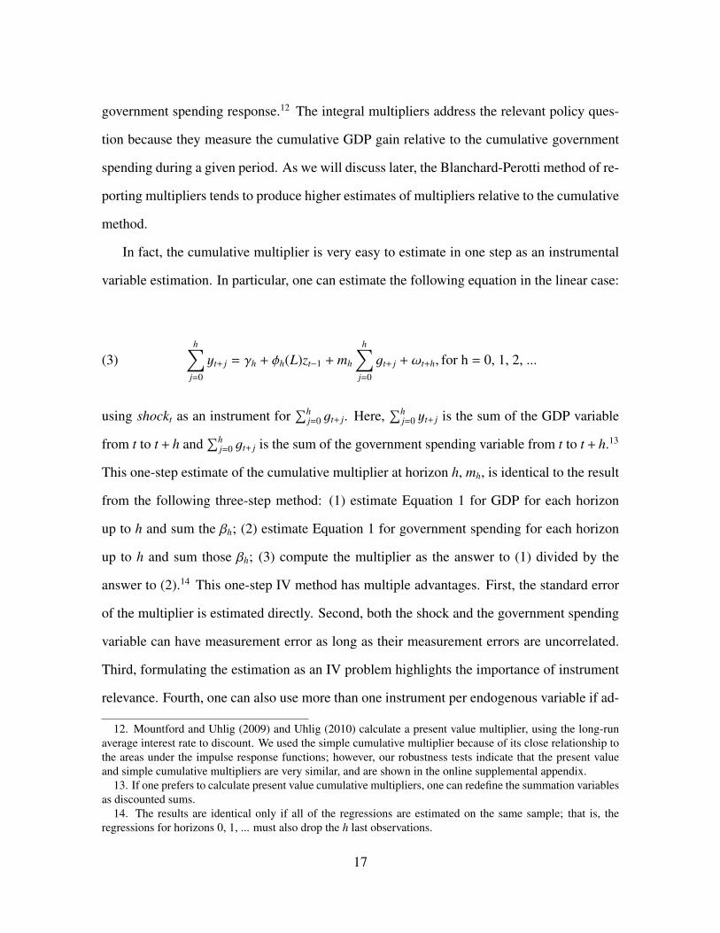
In fact, the cumulative multiplier is very easy to estimate in one step as an instrumental

variable estimation. In particular, one can estimate the following equation in the linear case:

(3)h∑

j=0

yt+ j = γh + ϕh(L)zt−1 + mh

h∑j=0

gt+ j + ωt+h, for h = 0, 1, 2, ...

using shockt as an instrument for∑h

j=0 gt+ j. Here,∑h

j=0 yt+ j is the sum of the GDP variable

from t to t + h and∑h

j=0 gt+ j is the sum of the government spending variable from t to t + h.13

This one-step estimate of the cumulative multiplier at horizon h, mh, is identical to the result

from the following three-step method: (1) estimate Equation 1 for GDP for each horizon

up to h and sum the βh; (2) estimate Equation 1 for government spending for each horizon

up to h and sum those βh; (3) compute the multiplier as the answer to (1) divided by the

answer to (2).14 This one-step IV method has multiple advantages. First, the standard error

of the multiplier is estimated directly. Second, both the shock and the government spending

variable can have measurement error as long as their measurement errors are uncorrelated.

Third, formulating the estimation as an IV problem highlights the importance of instrument

relevance. Fourth, one can also use more than one instrument per endogenous variable if ad-

12. Mountford and Uhlig (2009) and Uhlig (2010) calculate a present value multiplier, using the long-runaverage interest rate to discount. We used the simple cumulative multiplier because of its close relationship tothe areas under the impulse response functions; however, our robustness tests indicate that the present valueand simple cumulative multipliers are very similar, and are shown in the online supplemental appendix.

13. If one prefers to calculate present value cumulative multipliers, one can redefine the summation variablesas discounted sums.

14. The results are identical only if all of the regressions are estimated on the same sample; that is, theregressions for horizons 0, 1, ... must also drop the h last observations.

17

ditional instruments are available. This can be useful since the leading government spending

shocks tend to be relevant at different horizons. In subsequent sections, we show multipliers

that are estimated using military news shocks and Blanchard-Perotti shocks separately, as

well as in combination.

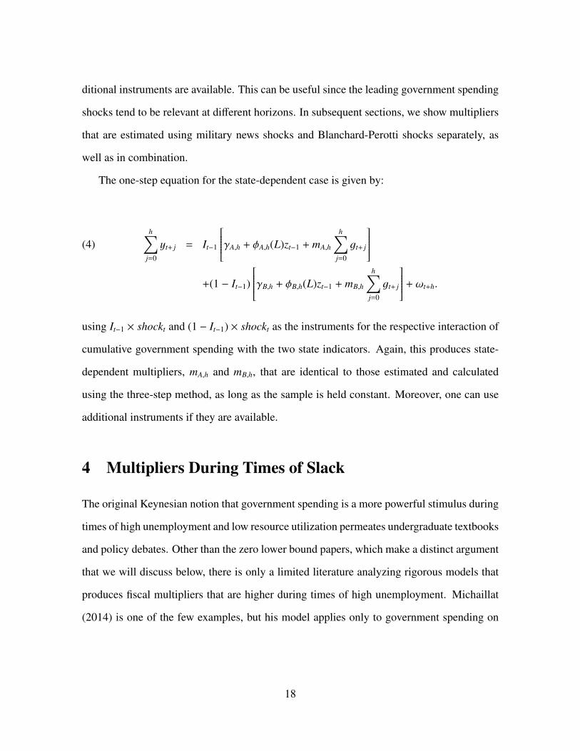
The one-step equation for the state-dependent case is given by:

h∑j=0

yt+ j = It−1

γA,h + ϕA,h(L)zt−1 + mA,h

h∑j=0

gt+ j

(4)

+(1 − It−1)

γB,h + ϕB,h(L)zt−1 + mB,h

h∑j=0

gt+ j

+ ωt+h.

using It−1 × shockt and (1 − It−1) × shockt as the instruments for the respective interaction of

cumulative government spending with the two state indicators. Again, this produces state-

dependent multipliers, mA,h and mB,h, that are identical to those estimated and calculated

using the three-step method, as long as the sample is held constant. Moreover, one can use

additional instruments if they are available.

4 Multipliers During Times of Slack

The original Keynesian notion that government spending is a more powerful stimulus during

times of high unemployment and low resource utilization permeates undergraduate textbooks

and policy debates. Other than the zero lower bound papers, which make a distinct argument

that we will discuss below, there is only a limited literature analyzing rigorous models that

produces fiscal multipliers that are higher during times of high unemployment. Michaillat

(2014) is one of the few examples, but his model applies only to government spending on

18

public employment.15 Thus, there is still a gap between Keynes’ original notion and modern

theories.

In this section, we analyze the issue empirically. Section 4.1 discusses our measure

of slack and shows graphs of the data and periods of slack. Section 4.2 presents statistics

showing the relevance of the military news shock, the Blanchard-Perotti shock, and their

combination at various horizons. Section 4.3 presents the main results. Section 4.4 conducts

robustness checks.

4.1 Measurement of Slack States

There are various potential measures of slack, such as output gaps, the unemployment rate,

or capacity utilization. Based on data availability and the fact that it is generally accepted

as a key measure of underutilized resources, we use the unemployment rate as our baseline

indicator of slack. We define an economy to be in a slack state when the unemployment rate

is above some threshold. For our baseline results, we follow Owyang et al. (2013) and use

6.5 as the threshold.16 We also conduct various robustness checks using different thresholds.

Note that our use of the unemployment rate to define the state is different from using

NBER recessions or Auerbach and Gorodnichenko’s (2012) moving average of GDP growth.

The latter two measures, which are highly correlated, indicate periods in which the economy

is moving from its peak to its trough. A typical recession encompasses periods in which

unemployment is rising from its low point to its high point, and hence is not an indicator of

a state of slack. Only half of the quarters that are official recessions are also periods of high

unemployment.

15. Numerous papers explore theoretically the possibility of state-dependent multipliers that depend onalternative states, such as the debt-to-GDP ratio, the condition of the financial system, degree of openness andexchange rate regimes. For example, see Corsetti et al. (2012) for a brief survey of this literature, as well asCanzoneri et al. (2016) and Sims and Wolff (2013).

16. They chose that threshold based on the U.S. Federal Reserve’s use of that threshold in its policy an-nouncements at the time. Barro and Redlick (2011) used 5.57 as the threshold, based on the median unemploy-ment rate from 1914 through 2006.

19

Figure 3 shows the unemployment rate, the military spending news shocks, and the es-

timated Blanchard-Perotti (BP) shocks. The largest military spending news shocks are dis-

tributed across periods with a variety of unemployment rates. For example, the largest news

shocks about WWI and the Korean War occurred when the unemployment rate was below

the threshold. In contrast, the initial large news shocks about WWII occurred when the un-

employment rate was still very high. The BP shocks tend to have large swings around wars.

However, they also have substantial volatility at other times. Some of this volatility in the

historical periods may be due to measurement error in the constructed government spending

series, though.

4.2 Instrument Relevance Across States of Slack

As discussed in the last section, multiplier estimates are the outcome of instrumental vari-

ables regressions. Because the military news variable is based on changes in defense spend-

ing due to political events, it should be exogenous to the economy. The question remains,

however, whether it is a relevant instrument. The standard rule-of-thumb is that an F-statistic

below 10 indicates a potential problem with instrument relevance (Staiger and Stock (1997)).

However, Olea and Pflueger (2013) show that the threshold can be different, and sometimes

higher, when the errors are serially correlated. Since there is inherent serial correlation

based on using the Jordà method, we use the Olea and Pflueger (2013) effective F-statistics

and thresholds.17

Figure 4 shows the difference between the first-stage effective F-statistics and the Olea

and Pflueger (2013) thresholds.18 A value above 0 means that the effective F-statistic exceeds

17. Even at horizon 0, we detected some serial correlation. Thus, we used automatic bandwidth selection atall horizons.

18. We use the threshold for the 5 percent critical value for testing the null hypothesis that the TSLS biasexceeds 10 percent of the OLS bias. For one instrument, this threshold is always 23.1. The threshold is 19.7percent for the ten percent critical value. The effective F-statistics and thresholds were calculated using Pfluegerand Wang (2015) Stata command "weakivtest."

20

the threshold. The F-statistics are from the regression of the sum of real government spending

from t to t + h on the shock(s) at t. The regression also includes all the other controls from

the second stage, which include lagged GDP, government spending and the news variable in

the case of military news shock. For the Blanchard-Perotti shock specification, current and

lagged military news are not included. The figure shows these for the full historical sample,

the historical sample excluding World War II, and the post-WWII sample, and splits each of

these according to whether the unemployment rate is above 6.5 percent. When we exclude

WWII, we exclude observations when either the dependent variable, the shock or the lagged

control variables occurs in the period 1941q3 through 1945q4. Rationing did not start until

1942q1, but Gordon and Krenn (2010) have argued that various other capacity constraints

occurred starting the second half of 1941. The results are shown for military news as the

instrument (solid line), for the Blanchard-Perotti shock as the instrument (dashed line), and

for both shocks as instruments.

Several features are evident from Figure 4. First, military news has potential relevance

problems at very short horizons whereas the Blanchard-Perotti shock has high relevance at

very short horizons. These results should be expected because the entire point of Ramey

(2011) is that the news about government spending occurs at least several quarters before the

government spending actually rises. In contrast, the Blanchard-Perotti shock is identified as

the part of current government spending not explained by the other lagged variables control

variables. Second, moving beyond the first year or two, the military news shock effective

F-statistic often rises above the threshold, whereas the Blanchard-Perotti shock one often

falls below the threshold.

Since the Blanchard-Perotti shock tends to do well at short horizons and the military

news at longer horizons, it is natural to consider using both shocks as instruments. The line

with stars in Figure 4 shows that when both shocks are used as instruments, the effective

F-statistics are above the threshold for more samples and horizons.

21

Note that none of the instrument alternatives has statistics above the threshold during

slack states in the post-WWII period for horizons beyond the two-year horizon. These results

support our initial conjecture that the post-WWII sample is not sufficiently rich to be able to

distinguish multipliers across states very precisely.

Using both shocks as instruments may come at a cost of exogeneity, though, since even

conditioning on lagged military news, the Blanchard-Perotti shock may be anticipated. Fur-

thermore, the likely measurement error in the historical government spending series will

be highly correlated with the Blanchard-Perotti shock, since the shock is equal to the fore-

cast error of government spending. As we shall see, the multiplier estimates that use the

Blanchard-Perotti shock are noticeably lower than those estimated using the military news

shock, consistent with attenuation bias from measurement error.

Because of possible problems with instrument relevance for some samples and some

horizons, we will also conduct some key hypothesis tests using Anderson and Rubin (1949)

statistics, which are robust to weak instruments. These tests have lower power, though.

4.3 Baseline Results for Slack States

We now present the main results of our analysis using the full historical sample and the

local projections method. Figure 5 shows the impulse response functions. We first consider

results from the linear model, which assumes that multipliers are invariant to the state of the

economy. The second column of Figure 5 shows the responses of government spending and

output to a military news shock in the linear model. The bands are 95 percent confidence

bands and are based on Newey-West standard errors that account for serial correlation. After

a shock to news, output and government spending begin to rise and then peak at around 12

quarters.

We compute cumulative multipliers for a two-year and four-year horizon, using mh from

Equation 3. As indicated in the first column of the top panel of Table 1, the implied multi-

22

pliers are around 0.7.

The main question addressed in this paper is whether the multipliers are state-dependent,

and in particular, whether they are high during periods of slack. The impulse response func-

tions in the state-dependent case are derived from the estimated βA,h and βB,h for Y and G in

Equation 2. The last column of Figure 5 shows the responses when we estimate the state-

dependent model where we distinguish between periods with and without slack in the econ-

omy. Similar to many pre-existing studies (e.g. Auerbach and Gorodnichenko (2012)), we

find that output responds more robustly during high unemployment states. However, govern-

ment spending also has a stronger response during those high slack periods. Consequently,

the larger output response during the high unemployment state does not imply a larger gov-

ernment spending multiplier. In fact, as shown in the second and third columns of Table 1,

the implied 2 and 4 year multipliers are very similar across the two states, both around 0.6 or

0.7. The final column shows the p-values for the test that the multiplier estimates differ across

states. The first p-value reported is based on heteroscedastic- and autocorrelation-consistent

(HAC) standard errors and is only valid for strong instruments; the second is based on the

Anderson and Rubin (1949) (AR) test and is robust to weak instruments.19 However, it has

lower power, so we prefer the HAC-based test for the sample-horizon combinations when

the instruments are strong. There is no evidence of differences in multipliers, either quanti-

tatively or statistically.

Figure 6 shows the cumulative multipliers for each horizon from impact to 5 years out.20

The top graph shows the linear model multipliers and the bottom graph shows the state de-

pendent multipliers. In the linear case, the cumulative multiplier in the first year is above

one but then falls. The reason for the higher initial multipliers after a news shock is given

19. We constructed the AR test conditional on the assumption that there was no instrument relevance problemfor the linear term in government spending and then tested the state-dependent term.

20. We only estimate multipliers out five years because the Jordà method is less reliable at long horizons.Thus, we may be neglecting the negative effects due to the eventual increase in distortionary tax, as highlightedby Drautzburg and Uhlig (2015).

23

by Ramey (2011): output responds immediately to news about future government spending

increases. Since output rises more quickly than government spending, the calculated mul-

tiplier looks large. The bottom graph shows that whatever the values, the multipliers in the

high unemployment state are below or equal to those in the low unemployment state.

The second panel of Table 1 shows alternative results using the Blanchard-Perotti (BP)

shock as the instrument.21 Estimated multipliers are lower in this case, 0.4 to 0.5 in the

linear case. Considering state dependence, multipliers are estimated to be higher in the

high unemployment state and even the AR test suggests some differences. However, the

estimates imply that multipliers differ across the states not because they are so elevated in

high unemployment states but because they are so low in low unemployment states. In all

cases, they are below unity.

There were two reasons why the BP shocks would be expected to yield lower estimates of

multipliers. First, as Ramey (2009) shows in DSGE Monte Carlo experiments, if the shocks

are anticipated, then the impulse responses will not capture the anticipatory rise in GDP. This

results in smaller multipliers. Second, as discussed in Section 2.2, there is likely significant

measurement error in the government spending series. Since the BP shock is defined as

the part of government spending not explained by lagged GDP and government spending, it

will inherit much of the measurement error. Thus, the measurement error in the instrument

will be correlated with the measurement error in government spending, so we should expect

attenuation bias in the multiplier estimate.

The third panel of Table 1 shows the estimated multipliers using both military news and

the BP shock as instruments. Recall that the combination of instruments had effective F-

statistics above the thresholds for all horizons when the full sample was used. The estimates

here are closer to those obtained using the BP shock alone, with most multipliers lower than

21. In these regressions, lagged news variables are excluded from the controls. The impulse responsefunctions are available in the online appendix. These IRFs also show both government spending and outputresponding more during high unemployment rate states. In contrast to the military news IRFs, governmentspending rises as soon as the shock hits.

24

those estimated for military news.22 There is a difference in multipliers using the HAC tests

(which are the preferred ones for strong instruments) at the four-year horizon. Again, though,

all multipliers are well below unity.

To summarize, across all three instruments sets we find multipliers that are less than 1

in all cases (beyond the first couple of quarters). Considering state dependence, we find no

evidence of sizeable multipliers in the periods of slack; the differences across states for the

BP shock stem from multipliers being so low during non-slack states.

4.4 Robustness of Slack Estimates

Our baseline results are potentially sensitive to the numerous specification choices we made

that were not guided by theory. Thus, in this section we explore the sensitivity of our findings

to these choices.

We begin by conducting robustness checks by changing the definition of the slack state.

We first allow for a time-varying threshold, where we consider deviations from trend for a

Hodrick-Prescott filtered unemployment rate.23 This definition of threshold results in about

50 percent of the observations being above the threshold . As shown in Figure 7, this thresh-

old also suggests prolonged periods of slack both in the late 1890s and during the 1930s.

There is substantial evidence that the "natural rate" of unemployment displayed an inverted

U-shape in the post-WWII period, and this time-varying threshold also helps account for

this. Using this time-varying threshold, we find results in line with our baseline findings:

multipliers less than one for the state-dependent case, no significant difference between the

multipliers when military news is used as the instrument, but some evidence of a difference

22. A test of over-identifying restrictions using the Hansen J-statistic rejects the restrictions in the linear caseat all horizons; the p-values (not shown in the table) range from 0.03 to 0.05. On the other hand, we cannotreject the overidentifying restrictions for the state-dependent model; the p-values range from 0.09 to 0.17 fornon-slack periods and 0.3 to 0.9 for slack periods.

23. We use a very high smoothing parameter of λ = 1, 000, 000, but even with this the Great Depression andWorld War II have a big influence. Thus, we fit the HP filter over a split sample, 1889 - 1929 and 1947 - 2015and linearly interpolate the small gap in trend unemployment between 1929 and 1947.

25

when the BP shock is used (see the first panel of Table 2a).

Second, we analyze the effect of raising the unemployment rate cut-off for the threshold,

to allow for the possibility of state-dependence only for a higher degree of slack in the

economy. The second panel in Table 2a shows that when we choose the threshold for the

unemployment rate to be higher than 8 percent, the slack state multiplier rises slightly to 0.8

for military news and to 0.7 for BP. Otherwise, the results are similar to the baseline.

We also consider NBER recession periods and smooth transition threshold based on 7-

quarter moving average of output growth, as in Auerbach and Gorodnichenko (2012).24 Re-

sults in the bottom panel of Table 2a show that in both cases we still get multipliers less than

one across both recession and expansion regimes, and do not find any evidence of higher

multipliers in recessions versus expansions. In fact, for Blanchard-Perotti shocks, the multi-

pliers are statistically significantly higher in expansions than in NBER recessions.

In order to account for the role of financing, we control for taxes by adding lags of the

average tax rate, given by tax revenues as a ratio of GDP, to our specification. The top panel

of Table 2b shows that our baseline results for both type of shocks are robust to the inclusion

of taxes. We have also conducted further analysis considering the role of financing, which is

detailed in the online appendix. This analysis shows that the behavior of deficit and taxes do

not seem to explain why multipliers are not higher during times of slack.

We next consider different samples. As discussed in the earlier case study, rationing was

a confounding influence during part of WWII. In order to determine whether our results are

sensitive to the constraints or the rationing, we exclude WWII from our sample.25 Recall

from Section 4.2, though, that all instrument sets appear to be weak for the high unemploy-

ment rate state for horizons beyond two years if this period is excluded. The third panel

of Table 2b shows that multipliers rise to around 1, and are even 1.6 in the case of BP at

24. We use the same definition as in Auerbach and Gorodnichenko (2012) and the online appendix showsthis smooth transition function for our historical sample.

25. See Section 4.2 for details on how we exclude WWII from our sample.

26

the 4 year horizon.26 However, the confidence bands are so large that there is no statisti-

cally significant difference (even at the 10 percent level) between multipliers across the two

states.27

The pre-existing literature on state-dependence of multipliers typically employs a shorter

data sample that spans the post World War II period.28 As a robustness check we limit our

sample to this period, 1947-2015, and the results are shown in the bottom panel of Table

2b. The multipliers in the linear case are similar to those in the full historical sample. In the

state dependent case the multipliers are estimated to be negative in the high unemployment

rate states, both for the military news shock and the BP shock. In both cases, the impulse

response of GDP is negative at most horizons, but even the HAC-based standard error bands

are very wide (not shown). However, recall that neither instrument was strong for the high

unemployment rate state in the post-WWII sample. Thus, the state-dependent estimates are

not reliable.

We also conducted a number of other robustness checks, such as using data based on

linear interpolation and including additional controls. The results are available in the online

appendix.

5 Multipliers at the Zero Lower Bound

We now investigate whether government spending multipliers differ when government in-

terest rates are near the zero lower bound or are being held constant to accommodate fiscal

26. Exclusion of WWII and the use of military news shocks is the one instance where the slight changesin sample make a difference in the multipliers calculated by summing impulse response functions versus es-timating things using the one-step method. The results shown are based on summing the impulse responsefunctions.

27. The confidence bands are not shown here. The BP multiplier estimate at the four-year horizon of 1.6during recessions has a HAC standard error above 1.9, so the estimate is not even significantly different fromzero.

28. See e.g. Bachmann and Sims (2012), Auerbach and Gorodnichenko (2012), Caggiano et al. (2015) andRiera-Crichton et al. (2015).

27

policy. Some New Keynesian models suggest that government spending multipliers will be

substantially higher (e.g. above 2) when the economy is at the zero lower bound.29 This

view has been challenged by a series of new papers, some of which construct models in

which multipliers are lower at the zero lower bound.30 Thus, the literature now provides a

number of plausible theories that predict both higher and lower multipliers at the zero lower

bound. For this reason, it is useful to provide empirical evidence on this issue.

Very few papers have attempted to test the predictions of the theory empirically in aggre-

gate data. Ramey (2011) estimates her model for the U.S. over the sub-sample from 1939

through 1951 and shows that the multiplier is no higher during that sample. Crafts and Mills

(2013) construct defense news shocks for the U.K. and estimate multipliers on quarterly data

from 1922 through 1938. They find multipliers below unity even when interest rates were

near zero.31

5.1 Defining States by Monetary Policy

The bottom panel of Figure 8 shows the behavior of three-month Treasury Bill rates from

1920 through the present, where the shortened sample is based on data availability, as well

as the discount rate for the period starting in 1914 until 1919 (dotted line) at the founding of

the Fed. The Treasury bill interest rate was near zero during much of the 1930s and 1940s, as

well as starting again in the fourth quarter of 2008. To indicate the degree to which interest

rates were pegged (either by design or the zero lower bound), we compare the behavior of

actual interest rates to that prescribed by the Taylor rule. We use the standard Taylor rule

29. See, for example, Eggertsson (2011) and Christiano et al. (2011). The relationship between governmentspending multipliers and the degree of monetary accommodation, even outside zero lower bound has beenexplored by many others, including Davig and Leeper (2011) and Zubairy (2014).

30. See, for example, Mertens and Ravn (2014), Aruoba and Schorfheide (2013), Braun et al. (2013) andKiley (2014).

31. Bruckner and Tuladhar (2014) focus on local not aggregate multipliers for Japan, and find that the effectsof local spending are larger in the ZLB period, but only modestly. A recent paper by Miyamoto et al. (2016)extends our analysis to Japan and finds some evidence of higher multipliers at the ZLB.

28

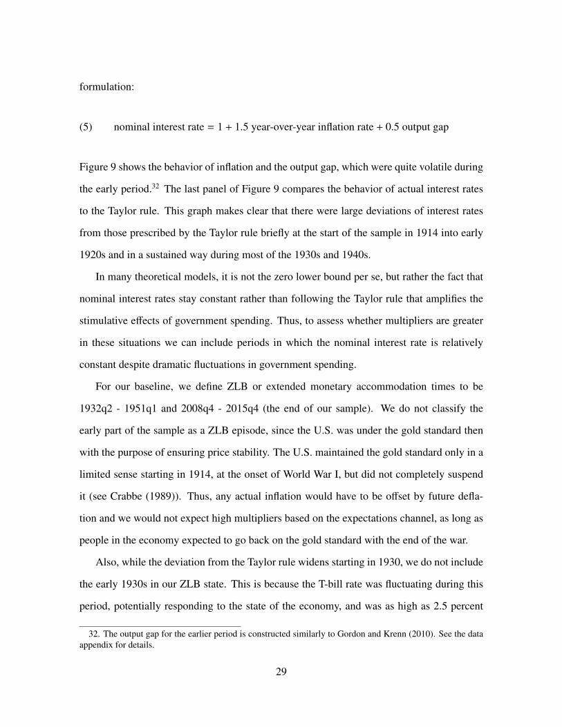
formulation:

(5) nominal interest rate = 1 + 1.5 year-over-year inflation rate + 0.5 output gap

Figure 9 shows the behavior of inflation and the output gap, which were quite volatile during

the early period.32 The last panel of Figure 9 compares the behavior of actual interest rates

to the Taylor rule. This graph makes clear that there were large deviations of interest rates

from those prescribed by the Taylor rule briefly at the start of the sample in 1914 into early

1920s and in a sustained way during most of the 1930s and 1940s.

In many theoretical models, it is not the zero lower bound per se, but rather the fact that

nominal interest rates stay constant rather than following the Taylor rule that amplifies the

stimulative effects of government spending. Thus, to assess whether multipliers are greater

in these situations we can include periods in which the nominal interest rate is relatively

constant despite dramatic fluctuations in government spending.

For our baseline, we define ZLB or extended monetary accommodation times to be

1932q2 - 1951q1 and 2008q4 - 2015q4 (the end of our sample). We do not classify the

early part of the sample as a ZLB episode, since the U.S. was under the gold standard then

with the purpose of ensuring price stability. The U.S. maintained the gold standard only in a

limited sense starting in 1914, at the onset of World War I, but did not completely suspend

it (see Crabbe (1989)). Thus, any actual inflation would have to be offset by future defla-

tion and we would not expect high multipliers based on the expectations channel, as long as

people in the economy expected to go back on the gold standard with the end of the war.

Also, while the deviation from the Taylor rule widens starting in 1930, we do not include

the early 1930s in our ZLB state. This is because the T-bill rate was fluctuating during this

period, potentially responding to the state of the economy, and was as high as 2.5 percent

32. The output gap for the earlier period is constructed similarly to Gordon and Krenn (2010). See the dataappendix for details.

29

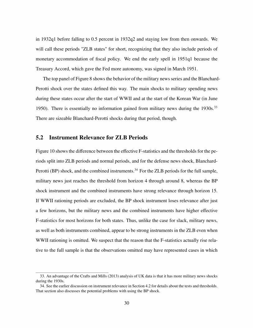
in 1932q1 before falling to 0.5 percent in 1932q2 and staying low from then onwards. We

will call these periods "ZLB states" for short, recognizing that they also include periods of

monetary accommodation of fiscal policy. We end the early spell in 1951q1 because the

Treasury Accord, which gave the Fed more autonomy, was signed in March 1951.

The top panel of Figure 8 shows the behavior of the military news series and the Blanchard-

Perotti shock over the states defined this way. The main shocks to military spending news

during these states occur after the start of WWII and at the start of the Korean War (in June

1950). There is essentially no information gained from military news during the 1930s.33

There are sizeable Blanchard-Perotti shocks during that period, though.

5.2 Instrument Relevance for ZLB Periods

Figure 10 shows the difference between the effective F-statistics and the thresholds for the pe-

riods split into ZLB periods and normal periods, and for the defense news shock, Blanchard-

Perotti (BP) shock, and the combined instruments.34 For the ZLB periods for the full sample,

military news just reaches the threshold from horizon 4 through around 8, whereas the BP

shock instrument and the combined instruments have strong relevance through horizon 15.

If WWII rationing periods are excluded, the BP shock instrument loses relevance after just

a few horizons, but the military news and the combined instruments have higher effective

F-statistics for most horizons for both states. Thus, unlike the case for slack, military news,

as well as both instruments combined, appear to be strong instruments in the ZLB even when

WWII rationing is omitted. We suspect that the reason that the F-statistics actually rise rela-

tive to the full sample is that the observations omitted may have represented cases in which

33. An advantage of the Crafts and Mills (2013) analysis of UK data is that it has more military news shocksduring the 1930s.

34. See the earlier discussion on instrument relevance in Section 4.2 for details about the tests and thresholds.That section also discusses the potential problems with using the BP shock.

30

the military news did not predict the actual path of government spending well.35

It is important to note that these effective F-statistic results depend heavily on our stan-

dard procedure of allowing the sample to change as the horizon advances. To be specific,

for the full sample with the WWII rationing periods excluded, as we go from horizon h to

h + 1, we drop two observations, one in the late 1930s or early 1940s and another near the

end of the sample in the 2010s. Dropping the extra observation in the 2010s makes no differ-

ence, but sometimes dropping an observation in the late 1930s or early 1940s does make a

difference because it means dropping a large military news shock. We considered fixing the

sample at the maximum horizon of 20 quarters, but that involves throwing away all observa-

tions for the 10-year period from 1936q3 through 1946q4. Not surprisingly, the F-statistics

for military news and the combined instruments are far below the threshold at virtually all

horizons if we discard the information during the entire 10-year period (not shown).

5.3 Results for ZLB States

To determine whether multipliers are different in ZLB states, we estimate our baseline state-

dependent model, but now allowing the state to be defined by monetary policy rather than

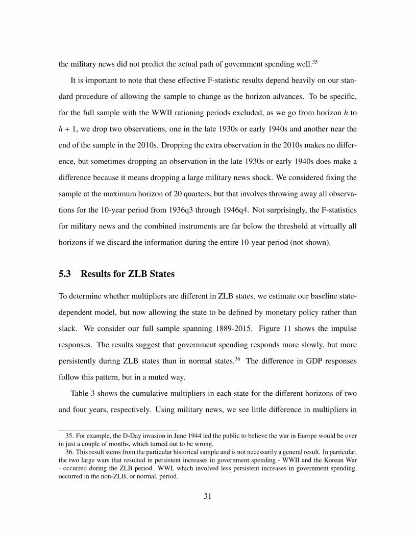
slack. We consider our full sample spanning 1889-2015. Figure 11 shows the impulse

responses. The results suggest that government spending responds more slowly, but more

persistently during ZLB states than in normal states.36 The difference in GDP responses

follow this pattern, but in a muted way.

Table 3 shows the cumulative multipliers in each state for the different horizons of two

and four years, respectively. Using military news, we see little difference in multipliers in

35. For example, the D-Day invasion in June 1944 led the public to believe the war in Europe would be overin just a couple of months, which turned out to be wrong.

36. This result stems from the particular historical sample and is not necessarily a general result. In particular,the two large wars that resulted in persistent increases in government spending - WWII and the Korean War- occurred during the ZLB period. WWI, which involved less persistent increases in government spending,occurred in the non-ZLB, or normal, period.

31

the ZLB state. Figure 12 shows the cumulative multiplier for the ZLB and normal state at

various different horizons along with 95% confidence bands. The multiplier for both states

is high on impact when the news shock hits the economy (since the shock is news about

future government spending) and is less than one after one year, but the multipliers across

the two states are never significantly different. For the BP shock and the combined shocks,

the multipliers are estimated to be 0.64 to 0.76 in the ZLB state, but only 0.1 to 0.26 in

the normal (non-ZLB) state. (See the middle and third panels of Table 3.) There is also

statistical evidence of differences in multipliers, as evidenced by the p-values; we reference

the HAC-based tests since the instruments appear to be strong. However, this difference is

due not to elevated multipliers in the ZLB but to multipliers estimated to be near 0 in the

normal states.

Table 4 shows various robustness checks. These robustness checks include redefining

the ZLB state periods to be where the T-bill rate was less than or equal to 50 basis points,

and including taxes and inflation as additional controls. The results show that our baseline

estimates are robust to these modifications. (See the online appendix for some additional

robustness checks)

We then explore the effect of excluding the capacity constraint and rationing periods

of WWII, excluding observations from the estimation if either the shock, the dependent

variable, or the lagged controls occurred in any quarter from 1941q3 through 1945q4. Table

5 shows the estimates.37 For the first time, we see evidence of multipliers above unity in a

"bad" state, in this case the ZLB state. Using military news as an instrument, the multiplier

is estimated to be 1.4 at two years and close to 1 at four years in the ZLB state. The BP

instrument also produces higher multiplier estimates in the ZLB state, though they have very

large standard errors. The multiplier estimates based on using both instruments, shown in

37. As in the case of slack, the excluded WWII sample along with the newsy shock leads to some differencesacross the 3-step and 1-step methods because of some influential observations in the changing sample. Thedifferences are smaller for the ZLB analysis, with the greatest differences being 0.2. We report the 1-stepestimates because it allows us also to use the combined instruments.

32

the lower panel of Table 5, imply a multiplier of 1.6 at the two-year horizon and 1.1 at the

four-year horizon. We can reject equality of the multipliers across states using the HAC-

based test, but not the AR test. Since the F-statistics are above the threshold, we prefer the

HAC-based test since it has better power. 38

In sum, when we consider the sample that excludes the rationing in WWII, we find

multipliers above unity at some horizons when we use the military news shock. That shock

used alone produces a multiplier estimate of 1.4, with a HAC standard error of 0.15, which

is statistically different from the one for normal times, estimated to be 0.6. Thus, in this

restricted sample we find both a multiplier above unity during ZLB periods and a difference

with normal periods. The online appendix shows that the multiplier estimates are above

unity at the two-year horizon for the military news shock also when we control for taxes and

inflation. The estimate during ZLB periods is 1.7, but it is estimated less precisely.

6 A Comparison of Methodologies and Estimates

In Section 4.3 we found no evidence of elevated multipliers during slack states. This result is

consistent with Barro and Redlick (2011), who also find no differences in contemporaneous

multipliers across states of slack. This finding stands in contrast, however, to the leading

study of state dependence for the U.S. by Auerbach and Gorodnichenko (2012) (AG-12)

who report multipliers as high as 2.5 for their definition of the recession state.

In this section, we show that the difference in results with AG-12 is largely driven by

the simplifying assumptions about state transitions that AG-12 use to convert their smooth

transition VAR (STVAR) estimates into impulse responses. We first explain the implicit as-

sumptions embedded in the Jordà method and compare them to the assumptions used by AG-

38. We also tested the over-identifying restrictions when we use the two instruments together. As discussedin a previous section, the over-identifying restrictions are rejected for the linear case. We cannot, however,reject them for the ZLB and normal states; the p-values for the ZLB states range from 0.2 to 0.8, depending onthe horizon, and for the normal states range from 0.14 to 0.27.

33

12. We next show that making their assumptions more consistent with their data-generating

process significantly reduces their recession-state multiplier estimates. Finally we apply a

threshold VAR (TVAR) method to our historical data in a way that is more consistent with

the data generating process and show that the estimates are very similar to those we obtained

using the Jordà method.

6.1 Methodological Differences with Auerbach-Gorodnichenko (2012)

The key ingredients for estimating multipliers in a dynamic environment are the impulse

responses of output and government spending. Constructing impulse responses in nonlinear

VAR models is far from straightforward since many complexities arise when one moves

from linear to nonlinear systems (e.g. Koop et al. (1996)). In a linear model, the impulse

responses are invariant to history, proportional to the size of the shock, and symmetric in

positive and negative shocks. In a nonlinear model, the response can depend differentially

on the magnitude and sign of the shock, as well as on the history of previous shocks. If

one estimates the parameters of a nonlinear model and then iterates on those parameters

to construct impulse responses, assumptions on how the economy transitions from state-

to-state, as well as how the shocks affect the state, are key components of the constructed

responses.

As discussed in Section 3.1, the Jordà method is similar to a direct forecasting method.

The impulse response estimate for GDP at t + h is a forecast of how GDP will differ at

t + h if shockt = 1 rather than shockt = 0. This means that if the average shock is likely

to change the state, it will be reflected in the impulse response estimate. On the other hand,

natural transitions between states that are independent of the shock should be captured by the

state-dependent control variables; i.e., the coefficients on the state-dependent (and horizon-

specific) constant terms and lagged variables will embed information on the average behavior

of the economy to transition to the other state at future horizons.

34

In contrast, Auerbach and Gorodnichenko (2012) estimate a regime-switching VAR model,

which switches between one set of reduced-form VAR parameters for recessions and another

set for expansions.39 The difficulty comes in generating impulse responses from those param-

eters because one must make assumptions about when the parameter sets should switch from

one state to the other. AG-12 calculate their baseline impulse responses under the assumption

that the economy stays in its current state for at least the 20 quarters over which they com-

pute their multiplier. This may be a reasonable approximation for expansions, which last for

several years, but it is not a good approximation for recession states, which have a mean du-

ration of only 3.3 quarters, according to their moving average of growth rates definition.40 In

fact, Hamilton (1989) has argued that GDP is well-described by a regime switching model

with a short-duration low growth regime ("recession") and a longer-duration high growth

regime ("expansion"). AG-12 estimate the 5-year multipliers in recessions to be 2.24, but

this high recession multiplier is not due to differences in impact effects on output, for those

are estimated to be equal across states (around 0.5). Rather, their high multiplier stems from

their constructed impulse response for the subsequent path of GDP after a shock hits in a

recession state. As the bottom left graph of Figure 2 of their paper (also reproduced in our

online appendix) shows, their constructed impulse response for GDP keeps rising indefi-

nitely after a spending shock hits during a recession, even though government spending does

not continue to rise. A regime-switching model for GDP provides a ready explanation for

their unusual response of output: on average, recessions do not last long, so during a reces-

sion one should forecast output growth in the next few years to be higher than current output

growth. Because their method assumes that the economy continues in recession indefinitely,

it looks like future growth will always be higher than current growth. With their method, the

39. They assume that the transitions across states are smooth, and the indicator function of the state of theeconomy varies between a maximum of one (extreme recession) and zero (extreme expansion).

40. Even the Great Recession, which was not part of their estimation sample, lasted only nine quarters bytheir definition. And the nine-quarter duration is an overestimate, since AG-12 use only extreme recessions intheir calculations.

35

multiplier grows as the horizon grows since output keeps rising but government spending

does not.

To show how the methodology changes the multiplier estimate, we first use the Jordà

method on AG-12’s exact data, sample and identification scheme. When we do so, we es-

timate a 5-year cumulative multiplier of 0.84.41 Thus, the Jordà method does not produce

elevated multipliers during recessions on the AG-12 sample and specification. In the online

appendix, we show that the difference between the two methods is largely due to AG-12’s

baseline assumption that the recession-state VAR parameters should apply for a 20 quarter

period. We use AG-12’s STVAR parameter estimates to construct alternative impulse re-

sponses that allow the state to change endogenously, both with respect to the history of the

non-government spending shocks and to the government spending shocks. We find multi-

pliers in severe recessions that are around unity. Thus, their high estimated multiplier in

recessions disappears when we allow more data-consistent transitions from state to state.42

6.2 Threshold VAR Estimation on the Historical Data

The threshold VAR method is not intrinsically problematic because one can vary the assump-

tions when translating the reduced form TVAR estimates to impulse response functions.43

Also, alternative definitions of states or alternative samples may be consistent with the as-

sumption of non-changing states through reasonable horizons. For example, ZLB states tend

41. We find, however, that these results are not robust since almost any deviation from their exact specifi-cation results in negative multipliers during recessions. For example, if we omit the four lags of the movingaverage of GDP growth, use a backward-moving average of growth for the state, or use 4 instead of 3 lags ofthe endogenous variables, the results change significantly. Alloza (2014) conducts a much more systematicanalysis of the importance of the two-sided moving average filter and shows that the results are not robust inthe STVAR either.

42. In later work, Auerbach and Gorodnichenko (2013) use the Jordà method on OECD data. Our onlineappendix explains that it is likely that the manner in which they converted IRFs to multipliers raised theirmultiplier estimates substantially.

43. Threshold VARs with various methodologies to construct state dependent impulse response functionsand fiscal multipliers have been employed by Baum et al. (2012), Batini et al. (2012) and Fazzari et al. (2015).We explore the source of difference between our results and those of Fazzari et al. (2015) in the online appendix.

36

to last many years, so holding the state constant is not contrary to the data.

In this section, we apply the TVAR methodology along with AG-12’s baseline assump-

tions about the duration of states to the ZLB case. We find estimates that are exceedingly

close to those we obtained using the Jordà method. We also explore the effect of applying

their method to recession states and also find results similar to those we obtain using the

Jordà method.

In particular, we consider the following reduced form threshold-VAR,

(6) Yt = It−1ΨA(L)Yt−1 + (1 − It−1)ΨB(L)Yt−1 + ut

where, as before, I is a dummy variable that indicates the state of the economy when the

shock hits and ut ∼ N(0,Ω). We also assume that Ω = It−1ΩA + (1 − It−1)ΩB, and Ψ(L) is a

polynomial of order 4. In order to identify a military news shock we set Yt = [newst, gt, yt]

and in order to identify a Blanchard and Perotti shock, we set Yt = [gt, yt], before doing a

Cholesky decomposition. Here yt and gt are Gordon-Krenn transformations of output and

government spending, respectively.

First, we define the state based on whether the interest rates are subject to ZLB. In our

full sample, we have classified two episodes as ZLB or extended monetary accommodation

times, and both have a long duration. In fact, average duration of a ZLB period is about 52

quarters. Thus, in this case the assumption that the state lasts several years is data consistent

even if we compute 5 year multipliers, since an average news or spending shock is not likely

to cause the economy to leave its current state.

Table 6 shows the state dependent multipliers for the ZLB state for both the Jordà method

and the threshold VAR, assuming that the economy does not exit from its current state. The

two methodologies give surprisingly similar results, for both the military news and Blanchard

and Perotti identification, with multipliers between 0.6 and 0.8 in the ZLB state for the

37

full historical sample.44 Thus, when the TVAR method and AG-12’s assumptions about

constant states are applied to samples and horizons over which those assumptions are more

consistent, the results look very much like those from the Jordà method. Examination of the

impulse responses constructed from the TVAR (shown in the online appendix) reveals that

the response of output during the ZLB state has the more usual hump shape, in contrast to

AG-12’s ever-increasing path of output.

Although slack periods do not last as long as ZLB periods, even in the historical sample,

it is still interesting to compare the estimates from the TVAR to those from the Jordà method

in that sample. We initially estimated the TVAR for our baseline definition of slack states, but

the roots were explosive. Thus, we explored the alternative of defining the state to be official

NBER recessions. The longest recession in the post-WWII sample lasted 6 quarters, but in

the historical sample there were four recessions that lasted 8 quarters or more. Table 6 shows

both the Jordà estimates and the estimates from the TVAR, assuming the economy does not

switch states. For the case of the military news shock, the multipliers are remarkably similar

across the two approaches. For the Blanchard-Perotti shock, the TVAR multiplier estimates

imply negative multipliers in recession and multipliers close to 0.4 in expansions. Thus, the

threshold-VAR approach also does not reveal any multiplier larger than 1 or provide any

evidence of larger multipliers in recessions than in expansion.

Overall, the threshold-VAR approach using the constant-state assumptions yields very

similar results to our baseline estimates using the Jordà approach. We find much more sim-

ilarity in the two methods in our application because all ZLB states last many quarters, and

in our historical sample even the recession states last longer. Moreover, our small multiplier

estimates are more consistent with AG-12’s baseline assumption that the government spend-

ing shock cannot make the economy switch states. Thus, the AG-12 simplifying assumption

is a better approximation to the data in our application than in theirs.

44. Recall that the multipliers were higher when we excluded WWII rationing. We tried to estimate theTVAR on that restricted sample, but the roots were explosive.

38

7 Conclusion

In this paper, we have investigated whether government spending multipliers vary depending

on the state of the economy. In order to maximize the amount of variation in the data, we

constructed new historical quarterly data spanning more than 120 years in the U.S. We con-

sidered two possible indicators of the state of the economy: the amount of slack, as measured

by the unemployment rate, and whether interest rates were being held constant close to the

zero lower bound. Using a more data-consistent method for estimating state-dependent im-

pulse responses and better ways of calculating multipliers from them, we provided numerous

estimates of multipliers across different specifications.

Our results for slack states can be summarized as follows. We find no evidence of

large multipliers when the U.S. economy is experiencing substantial slack as measured by

the unemployment rate. All estimates indicate multipliers below unity. When we use the

Blanchard-Perotti shock identification, we find differences in multipliers across states of

slack, but only because the multipliers are very low in non-slack states. Our numerous ro-

bustness checks suggest that our results are not sensitive to variations in our specification.

How do we reconcile these results with the common belief that government spending

during WWII lifted the economy out of the Great Depression? Our results do not dispute

this notion, but instead reinterpret it. WWII government spending did help lift the economy

out of the Great Depression, not because multipliers were so large, but because the amount

of government spending was so great. Although multipliers may be modest in magnitude,

they are positive.

In our analysis of multipliers in zero lower bound interest rate states, we also find no

evidence that multipliers are greater than one at the zero lower bound in the full sample. The

results are mixed, however, when we exclude World War II from the sample. Our preferred

shock, the military news shock, indicates multipliers around 1.4 at the two-year horizon

39

and the estimates are reasonably precise. On the other hand, the Blanchard-Perotti shock

suggests multipliers just below one, but they are not precisely estimated.

We also conduct a comparison of the Jordà method to the threshold VAR method used by

Auerbach and Gorodnichenko (2012). We show that Auerbach and Gorodnichenko’s (2012)

results depend on a simplifying assumption that is not a good approximation for their sample.

We show that their recession-state multipliers estimates are much lower once we relax that

assumption. We then implement a threshold VAR on our sample and states, for which the

simplifying assumption is more consistent with the data, and find results very close to those

we estimated using the Jordà method.

Of course, our results come with many caveats. As discussed in the introduction, we are

forced to use data determined by the vagaries of history so we do not have a controlled ex-

periment. Because the military news shock measures only changes in defense spending, and

because the Blanchard-Perotti shock mixes all types of shocks to government purchases, our

results do not inform us about the size of multipliers on specific classes of government out-

lays, such as transfer payments or infrastructure spending. Moreover, because the episodes

we studied were characterized by certain paths of taxes, the results are not immediately ap-

plicable to the case of deficit-financed stimulus packages or fiscal consolidations.

40

Data Appendix

GDP and GDP deflator:

1947 - 2015: Quarterly data on chain-weighted real GDP, nominal GDP, and

GDP deflator from BEA NIPA (downloaded from FRED, March 25, 2016 revi-

sion).

1889 - 1946: Annual data from 1929 - 1946 from BEA NIPA (downloaded from

FRED, December 20, 2012 version). For 1889 - 1928, series Ca9 and Ca13 from

Table Ca9-19 in Historical Statistics of the United States, Earliest Times to the

Present: Millennial Edition, Carter et al. (2006). These series are based on the

work of Kuznets, Kenrick, Gallman and Balke-Gordon.

1939 - 1946: We used seasonally adjusted quarterly nominal data on GNP from

National Income, 1954 Edition, A Supplement to the Survey of Current Business

and seasonally unadjusted CPI (all items, all urban consumers) from FRED.

1889 - 1938: Quarterly data on real GNP and GNP deflator. Source: Balke and

Gordon (1986). Data available at: http://www.nber.org/data/abc/

Data adjustment: For 1939-1946, we used a simplified version of the procedure

used by Valerie Ramey, "Identifying Government Spending Shocks: It’s All

in the Timing", Quarterly Journal of Economics, February 2011. We used the

quarterly nominal GNP series published in National Income, 1954 Edition, A

Supplement to the Survey of Current Business to interpolate the modern NIPA

annual nominal GDP series, and the quarterly averages of the CPI to interpolate

the NIPA annual GDP price deflator using the proportional Denton method. We

took the ratio to construct real GDP to use as a second round interpolator. We

spliced this quarterly real GDP series to the Balke-Gordon quarterly real GNP

series from 1889 - 1938 and used the combined series to interpolate the annual

41

real GDP series (described above) using the proportional Denton method. This

method insures that all quarterly real GDP series average to the annual series.

We used the Balke-Gordon deflator to interpolate the annual deflator series from

1889 - 1938 and combined it with the CPI-interpolated series from 1939-1946.

Finally, we linked the earlier series to the modern quarterly NIPA series from

1947 to the present.

Potential GDP:

The real GDP time trend is estimated as a sixth degree polynomial for the loga-

rithm of GDP, from 1889q1 through 2015q4 excluding 1930q1 through 1946q4.

Somewhat lower degree and somewhat higher degree polynomials gave similar

results for multipliers. Our method of constructing real potential GDP is similar

to the method advocated by Gordon and Krenn (2010). They illustrate the prob-

lems that arise when one uses standard filters to estimate trends during samples

that involve the Great Depression and World War II, and advocate instead using

a piecewise exponential trend based on benchmark years. Our procedure is a

smoothed version of theirs. To derive nominal potential GDP, we multiplied real

potential GDP by the actual price level. To derive the output gap for the Taylor

rule, we used the difference between log actual real GDP and log potential.

Government Spending:

1947 - 2015: Quarterly data on nominal "Government Consumption Expendi-

tures and Gross Investment," from BEA NIPA (downloaded from FRED, March

25, 2016 revision).

1889 - 1946: NIPA annual nominal data from 1929 - 1946 (BEA Table 1.1.5,

line 21) is spliced to annual data from 1889-1928, Source: Kendrick (1961)

Table A-II.

42

1939 - 1946: Quarterly data on nominal government spending from National

Income, 1954 Edition, A Supplement to the Survey of Current Business is used

to interpolate the modern annual NIPA values.

1889 - 1938: Monthly data on federal budget expenditures. Source: NBER

MacroHistory Database.

http://www.nber.org/databases/macrohistory/contents/chapter15.html

m15005a U.S. Federal Budget Expenditures, Total 01/1879-09/1915

m15005b U.S. Federal Budget Expenditures, Total 11/1914-06/1933

m15005c U.S. Federal Budget Expenditures, Total 01/1932-12/1938

Data adjustment: The monthly series are spliced together (using a 12-month

average at the overlap year) and seasonally adjusted in Eviews using X-12. This

series includes not just government expenditures but also transfer payments,

and so the monthly interpolator series is distorted by large transfer payments

in different quarters. Thus, rather than using the series directly, we use it as

a monthly interpolator for the annual series which excludes transfers. Follow-

ing Gordon and Krenn (2010), to find these quarters, we calculated the monthly

log change in the interpolator, and whenever a monthly change of +40 percent

or more was followed by a monthly change of approximately the same amount

with a negative sign (and also symmetrically negative followed by positive), we

replaced that particular observation by the average of the preceding and suc-

ceeding months. These instances occurred for the following months: 1904:5,

1922:11, 1931:2, 1931:12, 1932:7, 1934:01, 1936:06, and 1937:06. In addition,

the first quarter of 1917 was adjusted. The jump in spending was so dramatic in

1917q2 that the interpolated series showed a decline in spending in 1917q1 even

though the underlying expenditure series showed an increase of 16 percent in

43

that quarter relative to the previous one. Thus, we replaced the value of 1917q1

with a value 16 percent higher than the previous quarter. Note that our use of

the proportional Denton method creates a bumpier series than an alternative that

uses the additive Denton method. However, the additive Denton method leads to

series that behave very strangely around large buildups and builddowns of gov-

ernment spending, so we did not use it. On the other hand, the alternative series

gave very similar results for the multiplier.

We seasonally adjust the monthly interpolator series, but the quarterly interpo-

lation still had some residual seasonality. So, we applied X-12 again to the

quarterly interpolated series for 1879q3-1938q4.

Military News:

The narrative underlying the series is available in Ramey (2016).

Population:

1890-2015: Annual population data, based on July of each year, were taken

from Historical Statistics of the United States Millennial Edition Online, Carter

et al. (2006) We used total population, including armed forces overseas for all

periods where available (during WWI and 1930 and after); otherwise we used

the resident population. For 1952 through the present we used the monthly series

available on the Federal Reserve Bank of St. Louis FRED database, "POP."

Data adjustment: For 1890 through 1951, we linearly interpolated the annual

data to obtain monthly series so that the annual value was assigned to July. We

then took the averages of monthly values to obtain quarterly series. We did the

same to convert the monthly FRED data from 1952 to the present.

44

Federal Tax Revenues and Federal Expenditure:

We create federal deficit series by subtracting our federal tax revenue series from

our federal expenditures series (note these are total expenditures, not just gov-

ernment purchases).

1947-2015: Quarterly data on nominal "Federal Government Current receipts,"

BEA Table 3.2, line 1, March 25, 2016 version. Note that all NIPA BEA data is

on an accrual basis.

Quarterly data for 1959q3 - 2015q4 are from Table 3.2, line 42 "Total Expen-

ditures." The period 1947q1 - 1959q2 didn’t show the total because one of the

elements was missing. Since the missing element ("net purchases of nonpro-

duced assets" line 46) is so small, we assume it was 0 and added up the other

elements (lines 43 + 44 +45 - 47) to get the total.

1879-1938: Monthly data on federal budget receipts. Source: NBER Macro-

History Database

http://www.nber.org/databases/macrohistory/contents/chapter15.html . These data

are on a cash basis.

m15004a U.S. Federal Budget Receipts, Total 01/1879-06/1933

m15004b U.S. Federal Budget Receipts, Total 07/1930-06/1940

m15004c U.S. Federal Budget Receipts, Total 07/1939-12/1962

Monthly data on federal expenditures. Source: NBER MacroHistory Database

m15005a U.S. Federal Expenditures, Total 01/1879-10/1914

m15005b U.S. Federal Expenditures, Total 11/1914-12/1931

45

m15005c U.S. Federal Expenditures, Total 01/1932-06/1937

m15005d U.S. Federal Expenditures, Total 07/1937-06/1939

m15005e U.S. Federal Expenditures, Total 07/1939-06/1945

m15005f U.S. Federal Expenditures, Total 07/1945-12/1946

1939-1946: Quarterly data on nominal federal receipts from National Income,

1954 Edition, A Supplement to the Survey of Current Business is used to interpo-

late the modern annual NIPA values. We construct the quarterly federal receipts

interpolator from federal personal taxes + total corporates taxes + total indirect

taxes. Expenditures are same source as receipts with expenditures = federal

purchases + total transfers.

1889-1928: Annual data on federal receipts and expenditures. Source: Histori-

cal Statistics - fiscal year basis (e.g. fiscal year 1890 starts July 1, 1889).

1929-1946: Annual data on nominal "Federal Government Current receipts,"

BEA Table 3.2, line 1, March 27, 2014 version. Annual data on nominal "Fed-

eral Expenditures," BEA Table 3.2, adding up lines 43 + 44 +45 + 46 - 47,

treating missing components as 0’s since they were small once they became

available, March 25, 2016 version.

Data adjustment: The monthly series are strung together (with the most recent

series used for overlap periods) and seasonally adjusted in Eviews using X-12.

The annual series is interpolated using the monthly data with the Denton pro-

portional method. Same adjustment for expenditures as for receipts. Note, we

seasonally adjust the monthly interpolator series, but the quarterly interpolation

still had some residual seasonality. So, we applied X-12 again to the quarterly

interpolated series for 1879q3-1938q4.

46

Unemployment rate:

1948-2015: Monthly civilian unemployment rate. Source: Federal Reserve

Bank of St. Louis FRED database, UNRATE

http://research.stlouisfed.org/fred2/series/UNRATE

Data adjustment: Quarterly series is constructed as the average of the three

months.

1890-1947: Annual civilian unemployment rate. Source: Weir (1992). We

adjusted the Weir series from 1933-1943 to include emergency workers from

Conference Board (1945).

1890-1929: NBER-based monthly recession indicators. Source: Federal Re-

serve Bank of St. Louis FRED database, USREC

http://research.stlouisfed.org/fred2/series/USREC.

1930-1946: Monthly civilian unemployment rate (including emergency work-

ers). Source: NBER MacroHistory Database

http://www.nber.org/databases/macrohistory/contents/chapter08.html

m08292a U.S. Unemployment Rate, Seasonally Adjusted 04/1929-06/1942

m08292a U.S. Unemployment Rate, Seasonally Adjusted 01/1940, 03/1940-

12/1946

1947: Monthly civilian unemployment rate (including emergency workers, sea-

sonally adjusted) Source: Geoffrey Moore, Business Cycle Indicators, Volume

II, NBER p. 122

Data adjustment: Monthly NBER recession data are used to interpolate annual

data using the Denton interpolation from 1890-1929. For 1930-1947 onwards

we use the monthly unemployment rate series to interpolate annual data using

the Denton proportional interpolation.

47

Interest rate:

1934-2015: Monthly 3 month Treasury bill. Source: Federal Reserve Bank of

St. Louis FRED database, TB3MS

http://research.stlouisfed.org/fred2/series/TB3MS.

1920-1933: Monthly 3 month Treasury bill. Source: NBER MacroHistory

Database

http://www.nber.org/databases/macrohistory/contents/chapter13.html

m13029a U.S. Yields On Short-Term United States Securities, Three-

Six Month Treasury Notes and Certificates, Three Month Treasury

01/1920-03/1934

m13029b U.S. Yields On Short-Term United States Securities, Three-

Six Month Treasury Notes and Certificates, Three Month Treasury

01/1931-11/1969

Data adjustment: Quarterly series is constructed as the average of the three

months.

48

References

Alloza, Mario, 2014. “Is Fiscal Policy More Effective in Uncertain Times or During Reces-

sions?” Working paper, University College London.

Anderson, T.W. and H. Rubin, 1949. “Estimation of the Parameters of a Single Equation

in a Complete System of Stochastic Equations.” Annals of Mathematical Statistics 20:

46–63.

Aruoba, S. Boragan and Frank Schorfheide, 2013. “Macroeconomic Dynamics Near the

ZLB: A Tale of Two Equilibria.” NBER Working Paper 19248.

Auerbach, Alan and Yuriy Gorodnichenko, 2012. “Measuring the Output Responses to

Fiscal Policy.” American Economic Journal: Economic Policy 4(2): 1–27.

Auerbach, Alan and Yuriy Gorodnichenko, 2013. “Fiscal Multipliers in Recession and

Expansion.” In Fiscal Policy After the Financial Crisis, edited by Alberto Alesian and

Francesco Giavazzi, pp. 63–98. University of Chicago Press.

Bachmann, Rudiger and Eric R. Sims, 2012. “Confidence and the transmission of gov-

ernment spending shocks.” Journal of Monetary Economics 59: 235–249.

Balke, Nathan and Robert J. Gordon, 1986. “Appendix B Data Tables.” In The

American Business Cycle: Continuity and Change, edited by Robert J. Gordon, p.

http://www.nber.org/data/abc/. University of Chicago Press.

Barro, Robert J. and Charles J. Redlick, 2011. “Macroeconomic Effects from Govern-

ment Purchases and Taxes.” Quarterly Journal of Economics 126(1): 51–102.

Batini, Nicoletta, Giovanni Callegari, and Giovanni Melina, 2012. “Successful Auster-

ity in the United States, Europe and Japan.” IMF Working Papers 12/190, International

Monetary Fund.

49

Baum, Anja, Marcos Poplawski-Ribeiro, and Anke Weber, 2012. “Fiscal Multipliers and

the State of the Economy.” Unpublished paper, IMF.

Blanchard, Olivier and Roberto Perotti, 2002. “An Empirical Characterization of the

Dynamic Effects of Changes in Government Spending and Taxes on Output.” Quarterly

Journal of Economics 117(4): 1329–1368.

Braun, R. Anton, Lena Mareen Korber, and Yuichiro Waki, 2013. “Small and orthodox

fiscal multipliers at the zero lower bound.” Working Paper 2013-13, Federal Reserve Bank

of Atlanta.

Bruckner, Marcus and Anita Tuladhar, 2014. “Local Government Spending Multipli-

ers and Financial Distress: Evidence from Japanese Prefectures.” Economic Journal,

124(581): 1279–1316.

Caggiano, Giovanni, Efrem Castelnuovo, Valentina Colombo, and Gabriela Nodari,

2015. “Estimating Fiscal Multipliers: News From A Non-linear World.” Economic Jour-

nal 125(584): 746–776.

Canzoneri, Matthew, Fabrice Collard, Harris Dellas, and Behzad Diba, 2016. “Fiscal

Multipliers in Recessions.” Economic Journal, 126(590): 75–108.

Carter, Susan B., Scott Sigmund Gartner, Michael R. Haines, Alan L. Olmstead,

Richard Sutch, Gavin Wright, and Richard Sutch, 2006. “Table Ca9-19 : Gross do-

mestic product: 1790-2002 [Continuous annual series].” In Historical Statistics of the

United States Millennial Edition Online. Cambridge University Press.

Christiano, Lawrence, Martin Eichenbaum, and Sergio Rebelo, 2011. “When Is the

Government Spending Multiplier Large?” Journal of Political Economy 119(1): 78 –

121.

50

Coenen, Günter and et al., 2012. “Effects of Fiscal Stimulus in Structural Models.” Amer-

ican Economic Journal: Macroeconomics 4(1): 22–68.

Cogan, John F., Tobias Cwik, John B. Taylor, and Volker Wieland, 2010. “New Key-

nesian versus Old Keynesian Government Spending Multipliers.” Journal of Economic

Dynamics and Control 34: 281–295.

Conference Board, The, 1945. The Economic Almanac 1945-46. New York, New York:

National Industrial Conference Board, Inc.

Corsetti, Giancarlo, Andre Meier, and Gernot Mueller, 2012. “What determines govern-

ment spending multipliers?” Economic Policy 27(72): 521–565.

Crabbe, Leland, 1989. “The international gold standard and U.S. monetary policy from

World War I to the New Deal.” Federal Reserve Bulletin (Jun): 423–440.

Crafts, Nicholas and Terence C. Mills, 2013. “Rearmament to the Rescue? New Esti-

mates of the Impact of SKeynesianT Policies in 1930s’ Britain.” The Journal of Economic

History 73(04): 1077–1104.

Davig, Troy and Eric M. Leeper, 2011. “Monetary-Fiscal Policy Interactions and Fiscal

Stimulus.” European Economic Review 55(2): 211–227.

Drautzburg, Thorsten and Harald Uhlig, 2015. “Fiscal Stimulus and Distortionary Taxa-

tion.” Review of Economic Dynamics 18(4): 894–920.

Eggertsson, Gauti B., 2011. “What Fiscal Policy is Effective at Zero Interest Rates?” NBER

Macroeconomics Annual 25: 59–112.

Farhi, Emmanuel and Ivan Werning, 2016. “Fiscal Multipliers: Liquidity Traps and Cur-

rency Unions.” Handbook of Macroeconomics, forthcoming.

51

Fazzari, Steven M., James Morley, and Irina Panovska, 2015. “State-dependent effects

of fiscal policy.” Studies in Nonlinear Dynamics & Econometrics 19(3): 285–315.

Fisher, Jonas D.M. and Ryan Peters, 2010. “Using Stock Returns to Identify Government

Spending Shocks.” The Economic Journal 120: 414–436.

Friedman, Milton, 1952. “Price, Income, and Monetary Changes in Three Wartime Peri-

ods.” American Economic Review 42(2): 612–625.

Gordon, Robert J. and Robert Krenn, 2010. “The End of the Great Depression: VAR

Insight on the Roles of Monetary and Fiscal Policy.” NBER Working paper 16380.

Hall, Robert E., 2009. “By How Much Does GDP Rise If the Government Buys More

Output?” Brookings Papers on Economic Activity Fall: 183–236.

Hamilton, James D, 1989. “A New Approach to the Economic Analysis of Nonstationary

Time Series and the Business Cycle.” Econometrica 57(2): 357–84.

Jordà, Òscar, 2005. “Estimation and Inference of Impulse Responses by Local Projections.”

American Economic Review 95(1): 161–182.

Kendrick, John D., 1961. Productivity Trends in the United States. Princeton New Jersey:

Princeton University Press for the National Bureau of Economic Research.

Kiley, Michael T., 2014. “Policy Paradoxes in the New Keynesian Model.” Finance and

Economics Discussion Series 2014-29, Board of Governors of the Federal Reserve Sys-

tem.

Koop, Gary, Hashem M. Pesaran, and Simon M. Potter, 1996. “Impulse Response Anal-

ysis in Nonlinear Multivariate Models.” Journal of Econometrics 74(1): 119–147.

52

McGrattan, Ellen R. and Lee E. Ohanian, 2010. “Does Neoclassical Theory Account for

the Effects of Big Fiscal Shocks: Evidence from World War II.” International Economic

Review 51(2): 509–532.

Mertens, Karel and Morten O. Ravn, 2014. “Fiscal Policy in an Expectations Driven

Liquidity Trap.” Review of Economic Studies 81(4): 1637–1667.

Michaillat, Pascal, 2014. “A Theory of Countercyclical Government Multiplier.” American

Economic Journal: Macroeconomics 6(1): 190–217.

Miyamoto, Wataru, Thuy Lan Nguyen, and Dmitriy Sergeyev, 2016. “Government

Spending Multipliers under the Zero Lower Bound: Evidence from Japan.” Working

paper.

Mountford, Andrew and Harald Uhlig, 2009. “What are the Effects of Fiscal Policy

Shocks?” Journal of Applied Econometrics 24: 960–992.

Nakamura, Emi and Jón Steinsson, 2014. “Fiscal Stimulus in a Monetary Union: Evi-

dence from US Regions.” American Economic Review 104(3): 753–92.

Newey, Whitney K and Kenneth D West, 1987. “A Simple, Positive Semi-definite, Het-

eroskedasticity and Autocorrelation Consistent Covariance Matrix.” Econometrica 55(3):

703–08.

Ohanian, Lee E., 1997. “The Macroeconomic Effects of War Finance in the United States:

World War II and the Korean War.” American Economic Review 87(1): 23–40.

Olea, Jose Luis Montiel and Carolin Pflueger, 2013. “A Robust Test for Weak Instru-

ments.” Journal of Business & Economic Statistics 31(3): 358–369.

53

Owyang, Michael T., Valerie A. Ramey, and Sarah Zubairy, 2013. “Are Government

Spending Multipliers Greater During Times of Slack? Evidence from 20th Century His-

torical Data.” American Economic Review 103(2): 129–34.

Pflueger, Carolin E. and Su Wang, 2015. “A Robust Test for Weak Instruments in Stata.”

Stata Journal 15(1): 216–225.

Ramey, Valerie A., 2009. “Identifying Government Spending Shocks: It’s All in the Tim-

ing.” Working paper 15464, National Bureau of Economic Research.

Ramey, Valerie A., 2011. “Identifying Government Spending Shocks: It’s All in the Tim-

ing.” Quarterly Journal of Economic 126(1): 51–102.

Ramey, Valerie A., 2013. “Government Spending and Private Activity.” In Fiscal Policy

After the Financial Crisis, edited by Alberto Alesian and Francesco Giavazzi, pp. 19–55.

University of Chicago Press.

Ramey, Valerie A., 2016. “Defense News Shocks, 1889–2015: Estimates Based on News

Sources.” Unpublished paper, University of California, San Diego.

Riera-Crichton, Daniel, Carlos A. Vegh, and Guillermo Vuletin, 2015. “Procyclical and

countercyclical fiscal multipliers: Evidence from OECD countries.” Journal of Interna-

tional Money and Finance 52(C): 15–31.

Romer, Christina D., 1999. “Changes in Business Cycles: Evidence and Explanations.”

Journal of Economic Perspectives 13(2): 23–44.

Sims, Eric and Jonathan Wolff, 2013. “The Output and Welfare Effects of Government

Spending Shocks over the Business Cycle.” NBER Working Paper 19749.

Staiger, Douglas and James H. Stock, 1997. “Instrumental Variables Regression with Weak

Instruments.” Econometrica 65(3): 557–586.

54

Stock, James H. and Mark Watson, 2007. “Why Has US Inflation Become Harder to

Forecast?” Journal of Money, Credit, and Banking 39(1): 3–33.

Uhlig, Harald, 2010. “Some Fiscal Calculus.” American Economic Review 100(2): 30–34.

Weir, David R., 1992. “A Century of U.S. Unemployment, 1890-1990: Revised Estiamtes

and Evidence for Stabilization.” In Research in Economic History, edited by Roger L.

Ransom, pp. 301–346. JAI Press.

Zubairy, Sarah, 2014. “On Fiscal Multipliers: Estimates from a Medium-Scale DSGE

Model.” International Economic Review, 55(1).

55

Table 1. Estimates of Multipliers Across States of Slack

Linear High Low P-value for differenceModel Unemployment Unemployment in multipliers

across statesMilitary news shock2 year integral 0.66 0.60 0.59 HAC=0.954

(0.067) (0.095) (0.091) AR=0.954

4 year integral 0.71 0.68 0.67 HAC=0.924

(0.044) (0.052) (0.121) AR=0.924

Blanchard-Perotti shock2 year integral 0.38 0.68 0.30 HAC=0.005

(0.111) (0.102) (0.111) AR =0.070

4 year integral 0.47 0.77 0.35 HAC=0.001

(0.110) (0.075) (0.107) AR =0.031

Combined2 year integral 0.41 0.62 0.33 HAC=0.099

(0.098) (0.098) (0.110) AR =0.228

4 year integral 0.56 0.68 0.39 HAC=0.019

(0.079) (0.054) (0.102) AR =0.167

Note: The values in brackets under the multipliers give the standard errors. HAC indicatesHAC-robust p-values and AR indicates weak instrument robust Anderson-Rubin p-values.

56

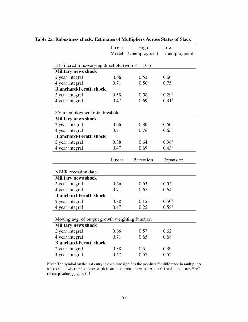
Table 2a. Robustness check: Estimates of Multipliers Across States of Slack

Linear High LowModel Unemployment Unemployment

HP filtered time-varying threshold (with λ = 106)Military news shock2 year integral 0.66 0.52 0.664 year integral 0.71 0.56 0.75Blanchard-Perotti shock2 year integral 0.38 0.58 0.29†

4 year integral 0.47 0.69 0.31†

8% unemployment rate thresholdMilitary news shock2 year integral 0.66 0.80 0.604 year integral 0.71 0.76 0.65Blanchard-Perotti shock2 year integral 0.38 0.64 0.36†

4 year integral 0.47 0.69 0.43†

Linear Recession Expansion

NBER recession datesMilitary news shock2 year integral 0.66 0.63 0.554 year integral 0.71 0.67 0.64Blanchard-Perotti shock2 year integral 0.38 0.15 0.50†

4 year integral 0.47 0.25 0.58†

Moving avg. of output growth weighting functionMilitary news shock2 year integral 0.66 0.57 0.624 year integral 0.71 0.65 0.68Blanchard-Perotti shock2 year integral 0.38 0.51 0.394 year integral 0.47 0.57 0.52

Note: The symbol on the last entry in each row signifies the p-values for difference in multipliersacross state, where * indicates weak instrument robust p-value, pAR < 0.1 and † indicates HAC-robust p-value, pHAC < 0.1.

57

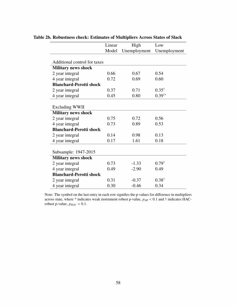
Table 2b. Robustness check: Estimates of Multipliers Across States of Slack

Linear High LowModel Unemployment Unemployment

Additional control for taxesMilitary news shock2 year integral 0.66 0.67 0.544 year integral 0.72 0.69 0.60Blanchard-Perotti shock2 year integral 0.37 0.71 0.35†

4 year integral 0.45 0.80 0.39†∗

Excluding WWIIMilitary news shock2 year integral 0.75 0.72 0.564 year integral 0.73 0.89 0.53Blanchard-Perotti shock2 year integral 0.14 0.98 0.134 year integral 0.17 1.61 0.18

Subsample: 1947-2015Military news shock2 year integral 0.73 -1.33 0.79†

4 year integral 0.49 -2.90 0.49Blanchard-Perotti shock2 year integral 0.31 -0.37 0.38†

4 year integral 0.30 -0.46 0.34

Note: The symbol on the last entry in each row signifies the p-values for difference in multipliersacross state, where * indicates weak instrument robust p-value, pAR < 0.1 and † indicates HAC-robust p-value, pHAC < 0.1.

58

Table 3. Estimates of Multipliers Across Monetary Policy Regimes

Linear Near Zero Normal P-value for differenceModel Lower Bound in multipliers across

states

BaselineMilitary news shock2 year integral 0.66 0.77 0.63 HAC=0.429

(0.067) (0.106) (0.149) AR =0.504

4 year integral 0.71 0.77 0.77 HAC=0.992

(0.044) (0.058) (0.376) AR =0.992

Blanchard-Perotti shock2 year integral 0.38 0.64 0.10 HAC=0.000

(0.111) (0.033) (0.112) AR =0.066

4 year integral 0.47 0.71 0.12 HAC=0.000

(0.110) (0.033) (0.115) AR =0.062

Combined2 year integral 0.41 0.67 0.26 HAC=0.000

(0.098) (0.027) (0.103) AR =0.184

4 year integral 0.56 0.76 0.21 HAC=0.000

(0.084) (0.040) (0.136) AR =0.208

Note: The values in brackets under the multipliers give the standard errors. HAC indicatesHAC-robust p-values and AR indicates weak instrument robust Anderson-Rubin p-values.

59

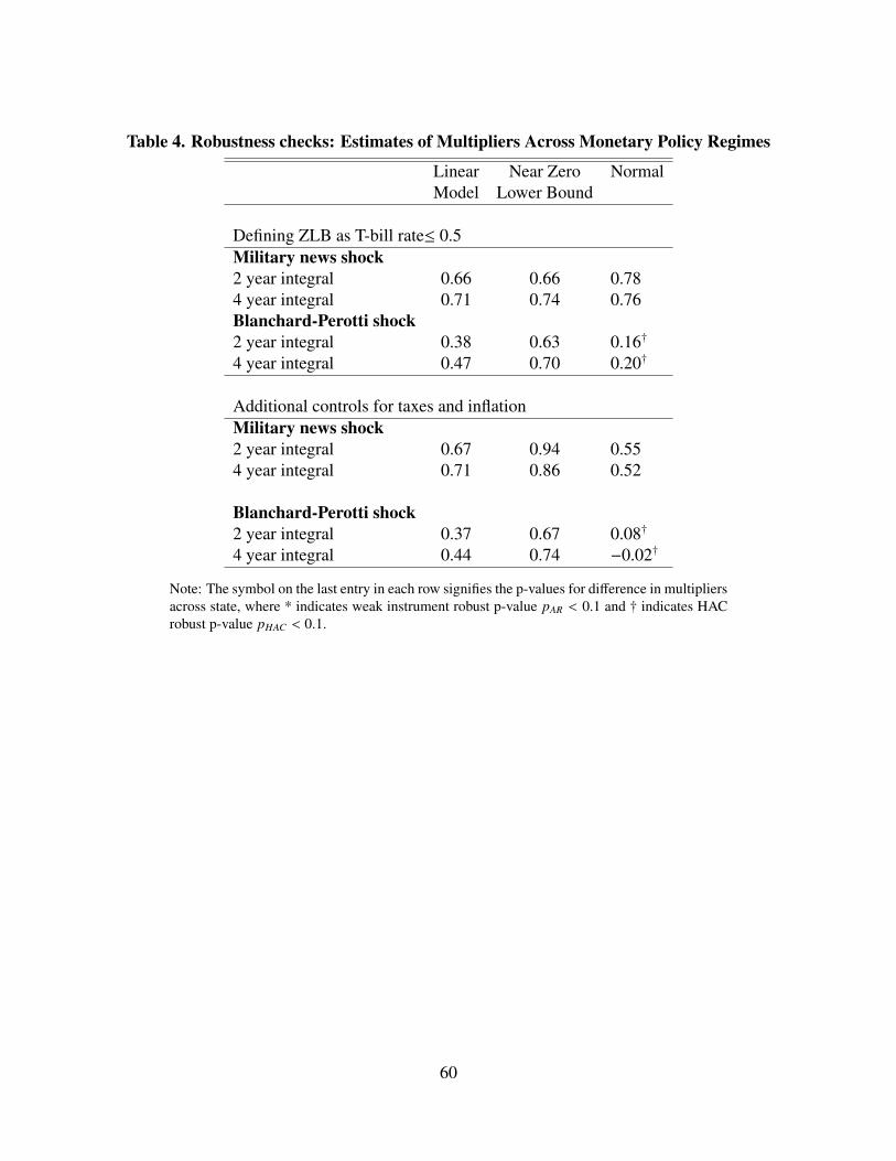
Table 4. Robustness checks: Estimates of Multipliers Across Monetary Policy Regimes

Linear Near Zero NormalModel Lower Bound

Defining ZLB as T-bill rate≤ 0.5Military news shock2 year integral 0.66 0.66 0.784 year integral 0.71 0.74 0.76Blanchard-Perotti shock2 year integral 0.38 0.63 0.16†

4 year integral 0.47 0.70 0.20†

Additional controls for taxes and inflationMilitary news shock2 year integral 0.67 0.94 0.554 year integral 0.71 0.86 0.52

Blanchard-Perotti shock2 year integral 0.37 0.67 0.08†

4 year integral 0.44 0.74 −0.02†

Note: The symbol on the last entry in each row signifies the p-values for difference in multipliersacross state, where * indicates weak instrument robust p-value pAR < 0.1 and † indicates HACrobust p-value pHAC < 0.1.

60

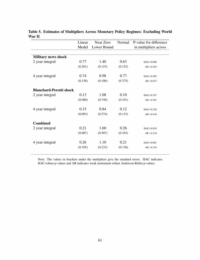
Table 5. Estimates of Multipliers Across Monetary Policy Regimes: Excluding WorldWar II

Linear Near Zero Normal P-value for differenceModel Lower Bound in multipliers across

Military news shock2 year integral 0.77 1.40 0.63 HAC=0.000

(0.201) (0.153) (0.152) AR =0.263

4 year integral 0.74 0.98 0.77 HAC=0.585

(0.158) (0.100) (0.375) AR =0.637

Blanchard-Perotti shock2 year integral 0.13 1.08 0.10 HAC=0.197

(0.080) (0.749) (0.101) AR =0.301

4 year integral 0.15 0.84 0.12 HAC=0.228

(0.093) (0.574) (0.115) AR =0.416

Combined2 year integral 0.21 1.60 0.26 HAC=0.010

(0.087) (0.507) (0.103) AR =0.216

4 year integral 0.26 1.10 0.21 HAC=0.001

(0.105) (0.233) (0.136) AR =0.354

Note: The values in brackets under the multipliers give the standard errors. HAC indicatesHAC-robust p-values and AR indicates weak instrument robust Anderson-Rubin p-values.

61

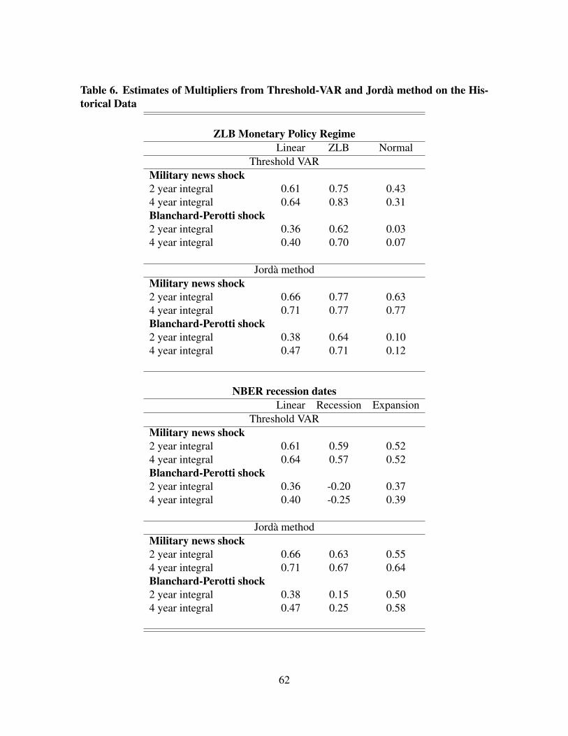
Table 6. Estimates of Multipliers from Threshold-VAR and Jordà method on the His-torical Data

ZLB Monetary Policy RegimeLinear ZLB Normal

Threshold VARMilitary news shock2 year integral 0.61 0.75 0.434 year integral 0.64 0.83 0.31Blanchard-Perotti shock2 year integral 0.36 0.62 0.034 year integral 0.40 0.70 0.07

Jordà methodMilitary news shock2 year integral 0.66 0.77 0.634 year integral 0.71 0.77 0.77Blanchard-Perotti shock2 year integral 0.38 0.64 0.104 year integral 0.47 0.71 0.12

NBER recession datesLinear Recession Expansion

Threshold VARMilitary news shock2 year integral 0.61 0.59 0.524 year integral 0.64 0.57 0.52Blanchard-Perotti shock2 year integral 0.36 -0.20 0.374 year integral 0.40 -0.25 0.39

Jordà methodMilitary news shock2 year integral 0.66 0.63 0.554 year integral 0.71 0.67 0.64Blanchard-Perotti shock2 year integral 0.38 0.15 0.504 year integral 0.47 0.25 0.58

62

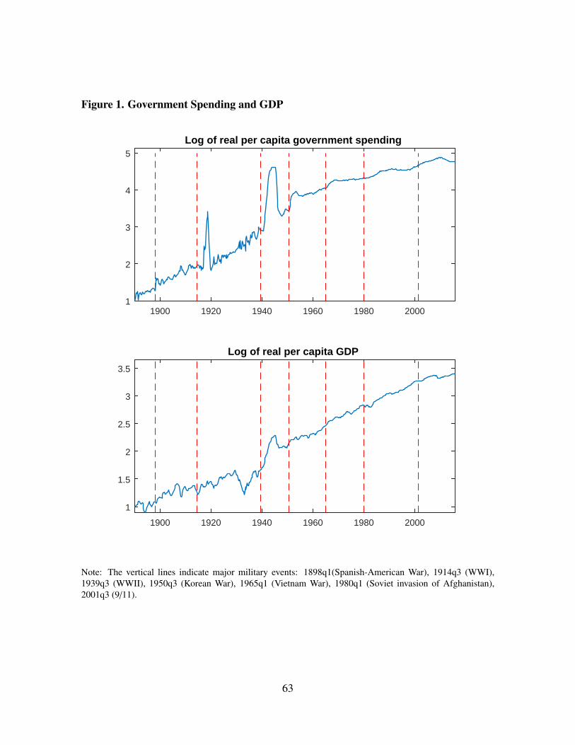
Figure 1. Government Spending and GDP

1900 1920 1940 1960 1980 20001

2

3

4

5

Log of real per capita government spending

1900 1920 1940 1960 1980 2000

1

1.5

2

2.5

3

3.5

Log of real per capita GDP

Note: The vertical lines indicate major military events: 1898q1(Spanish-American War), 1914q3 (WWI),1939q3 (WWII), 1950q3 (Korean War), 1965q1 (Vietnam War), 1980q1 (Soviet invasion of Afghanistan),2001q3 (9/11).

63

Figure 2. Evolution of variables during war episodes

1914 1916 1918 1920

rypr

iv

600

700

Private activity and Government spending

rgov

100

200

1914 1916 1918 1920

-10

0

10

20

30

Military news (% of GDP)

1914 1916 1918 1920

2

4

6

8

Unemployment rate

1938 1940 1942 1944 1946 1948

rypr

iv

1000

1500rg

ov

500

1000

1938 1940 1942 1944 1946 1948-20

0

20

40

60

1938 1940 1942 1944 1946 1948

5

10

15

1948 1950 1952 1954

rypr

iv

2000

rgov500

1948 1950 1952 1954

0

20

40

60

1948 1950 1952 1954

3

4

5

6

7

Note: The first column shows real private activity (left-axis) and real government spending (right axis). Thesecond column shows military spending news with shaded areas indicating periods we classify as the zerolower bound period for interest rate, and the third column shows the civilian unemployment rate. The first rowcorresponds to the period around World War I, the second row shows the time period around World War II andthe last row shows the period around the Korean war.

64

Figure 3. Military spending news, Blanchard-Perotti shock and unemployment rate

1900 1920 1940 1960 1980 2000-20

0

20

40

60

Military news (% of GDP)

1900 1920 1940 1960 1980 2000

-0.1

-0.05

0

0.05

Blanchard-Perotti shock

1900 1920 1940 1960 1980 2000

5

10

15

20

Unemployment rate

Note: Shaded areas indicate periods when the unemployment rate is above the threshold of 6.5%.

65

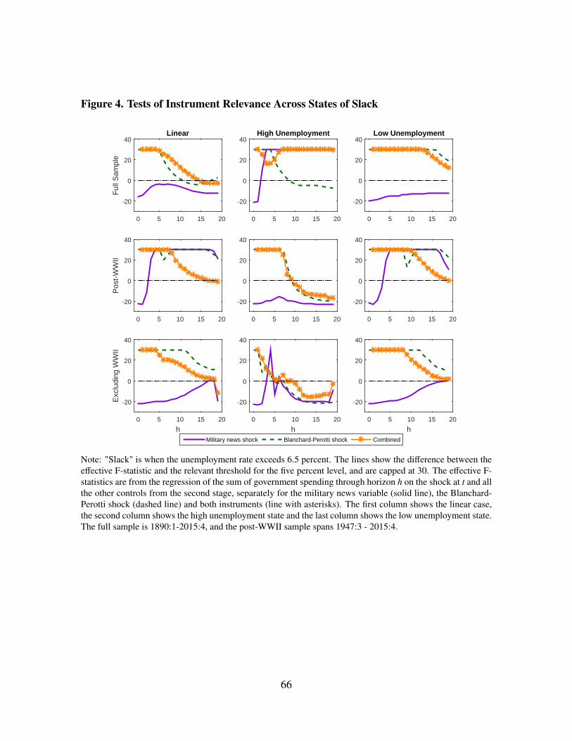
Figure 4. Tests of Instrument Relevance Across States of Slack

0 5 10 15 20

Ful

l Sam

ple

-20

0

20

40Linear

0 5 10 15 20

-20

0

20

40High Unemployment

0 5 10 15 20

-20

0

20

40Low Unemployment

0 5 10 15 20

Pos

t-W

WII

-20

0

20

40

0 5 10 15 20

-20

0

20

40

0 5 10 15 20

-20

0

20

40

h0 5 10 15 20

Exc

ludi

ng W

WII

-20

0

20

40

h0 5 10 15 20

-20

0

20

40

h0 5 10 15 20

-20

0

20

40

Military news shock Blanchard-Perotti shock Combined

Note: "Slack" is when the unemployment rate exceeds 6.5 percent. The lines show the difference between theeffective F-statistic and the relevant threshold for the five percent level, and are capped at 30. The effective F-statistics are from the regression of the sum of government spending through horizon h on the shock at t and allthe other controls from the second stage, separately for the military news variable (solid line), the Blanchard-Perotti shock (dashed line) and both instruments (line with asterisks). The first column shows the linear case,the second column shows the high unemployment state and the last column shows the low unemployment state.The full sample is 1890:1-2015:4, and the post-WWII sample spans 1947:3 - 2015:4.

66

Figure 5. Government spending and GDP responses to a news shock: Considering slackstates

5 10 15 20

Gov

ernm

ent s

pend

ing

0

0.2

0.4

0.6

5 10 15 20

0

0.2

0.4

0.6Linear

5 10 15 20

0

0.2

0.4

0.6

0.8

State-dependent

quarter5 10 15 20

GD

P

0

0.2

0.4

0.6

quarter5 10 15 20

0

0.1

0.2

0.3

0.4

quarter5 10 15 20

0

0.2

0.4

0.6

Linear

Low Unemp

High Unemp

Note: Response of government spending and GDP to a news shock equal to 1% of GDP. The top row showsthe response of government spending and the second row shows the response of GDP. The first column showsthe responses in the linear and state-dependent model. The second column shows the responses in the linearmodel. The last column shows the state-dependent responses where the blue dashed lines are responses in thehigh unemployment state and the lines with red circles are responses in the low unemployment state. 95%confidence intervals are shown in second and third columns.

67

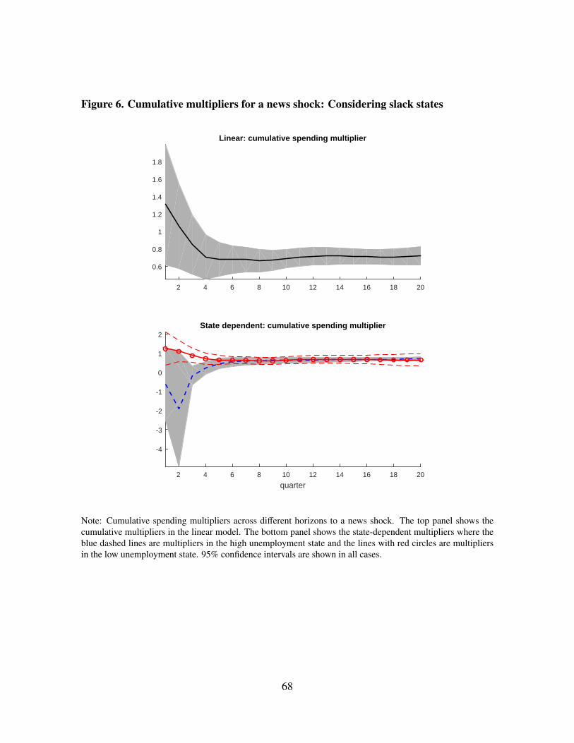
Figure 6. Cumulative multipliers for a news shock: Considering slack states

2 4 6 8 10 12 14 16 18 20

0.6

0.8

1

1.2

1.4

1.6

1.8

Linear: cumulative spending multiplier

quarter2 4 6 8 10 12 14 16 18 20

-4

-3

-2

-1

0

1

2State dependent: cumulative spending multiplier

Note: Cumulative spending multipliers across different horizons to a news shock. The top panel shows thecumulative multipliers in the linear model. The bottom panel shows the state-dependent multipliers where theblue dashed lines are multipliers in the high unemployment state and the lines with red circles are multipliersin the low unemployment state. 95% confidence intervals are shown in all cases.

68

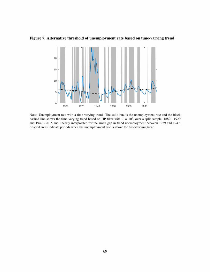
Figure 7. Alternative threshold of unemployment rate based on time-varying trend

1900 1920 1940 1960 1980 20000

5

10

15

20

Note: Unemployment rate with a time-varying trend. The solid line is the unemployment rate and the blackdashed line shows the time varying trend based on HP filter with λ = 106, over a split sample, 1889 - 1929and 1947 - 2015 and linearly interpolated for the small gap in trend unemployment between 1929 and 1947.Shaded areas indicate periods when the unemployment rate is above the time-varying trend.

69

Figure 8. Military spending news, Blanchard-Perotti shock and interest rate

1900 1920 1940 1960 1980 2000-20

0

20

40

60

Military news (% of GDP)

1900 1920 1940 1960 1980 2000

-0.1

-0.05

0

0.05

Blanchard-Perotti shock

1900 1920 1940 1960 1980 2000

5

10

153 month Treasury bill rate

Note: Shaded areas indicate periods which we classify as the zero lower bound period for interest rate.

70

Figure 9. Inflation, output gap and Taylor rule implied interest rate

1920 1930 1940 1950 1960 1970 1980 1990 2000 2010

-10

0

10

20

Inflation (year over year)

1920 1930 1940 1950 1960 1970 1980 1990 2000 2010

-40

-20

0

20

Output gap

1920 1930 1940 1950 1960 1970 1980 1990 2000 2010

-20

0

20

T-bill rate and Taylor rule int rate

Note: The top panel shows the year-over-year GDP deflator inflation rate and the second panel shows the outputgap, which is constructed as the percentage deviation between real GDP and potential GDP. In the last panel,the dashed line shows the Taylor-rule implied nominal interest rate, and the solid line shows the data for the3-month T-bill rate, with a dotted line for 1914-1919 showing the discount rate. In the last panel, the shadedareas indicate periods which we classify as the zero lower bound period for interest rate.

71

Figure 10. Tests of Instrument Relevance Across Monetary Policy Regimes

0 10 20

Ful

l Sam

ple

-30

-20

-10

0

10

20

30

40Linear

0 10 20-30

-20

-10

0

10

20

30

40ZLB

0 10 20-30

-20

-10

0

10

20

30

40Normal

h0 10 20

Exc

ludi

ng W

WII

-30

-20

-10

0

10

20

30

40

h0 10 20

-30

-20

-10

0

10

20

30

40

h0 10 20

-30

-20

-10

0

10

20

30

40

Military news shock Blanchard-Perotti shock Combined

Note: "ZLB" is when interest rates are near the zero lower bound or the Fed is being very accommodativeof fiscal policy (1932q1-1951q1, 2008q4-2015q4). The lines show the difference between the effective F-statistic and the relevant threshold for the five percent level, and are capped at 30. The effective F-statistics arefrom the regression of the sum of government spending through horizon h on the shock at t and all the othercontrols from the second stage, separately for the military news variable (solid line), the Blanchard-Perottishock (dashed line) and both instruments (line with asterisks). The first column shows the linear case, thesecond column shows the high unemployment state and the last column shows the low unemployment state.The full sample is 1890:1-2015:4.

72

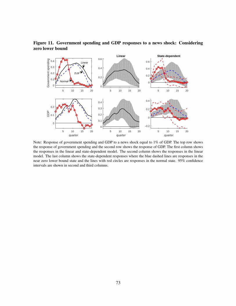
Figure 11. Government spending and GDP responses to a news shock: Consideringzero lower bound

5 10 15 20

Gov

ernm

ent s

pend

ing

0

0.1

0.2

0.3

0.4

5 10 15 20

0

0.2

0.4

0.6Linear

5 10 15 20

0

0.2

0.4

0.6

State-dependent

quarter5 10 15 20

GD

P

0

0.1

0.2

quarter5 10 15 20

0

0.1

0.2

0.3

0.4

quarter5 10 15 20

-0.2

0

0.2

0.4

Linear

ZLB

Normal

Note: Response of government spending and GDP to a news shock equal to 1% of GDP. The top row showsthe response of government spending and the second row shows the response of GDP. The first column showsthe responses in the linear and state-dependent model. The second column shows the responses in the linearmodel. The last column shows the state-dependent responses where the blue dashed lines are responses in thenear zero lower bound state and the lines with red circles are responses in the normal state. 95% confidenceintervals are shown in second and third columns.

73

Figure 12. Cumulative multipliers for a news shock: Considering zero lower bound

2 4 6 8 10 12 14 16 18 20

0.6

0.8

1

1.2

1.4

1.6

1.8

Linear: cumulative spending multiplier

quarter2 4 6 8 10 12 14 16 18 20

0

0.5

1

1.5

2

2.5

3

State dependent: cumulative spending multiplier

Note: Cumulative spending multipliers across different horizons for a news shock. The top panel shows thecumulative multipliers in the linear model. The bottom panel shows the state-dependent multipliers where theblue dashed lines are multipliers in the near zero-lower bound state and the lines with red circles are multipliersin the normal state. 95% confidence intervals are shown in all cases.

74