Embed Size (px)
Citation preview

ISSN 2385-2755
Working papers
(Dipartimento di scienze sociali ed economiche)
[online]
SAPIENZA – UNIVERSITY OF ROME P.le Aldo Moro n.5 – 00185 Roma T (+39) 06 49910563 F (+39) 06 49910231 CF 80209930587 - P.IVA 02133771002
WORKING PAPERS SERIES
DIPARTIMENTO DI
SCIENZE SOCIALI ED ECONOMICHE
n. 4/2015
Government spending and the exchange rate
Authors:
Giorgio Di Giorgio, Salvatore Nisticò, Guido Traficante
Revised version: January 2016

Government spending and the exchange rate∗
Giorgio Di GiorgioLUISS Guido Carli
Salvatore NisticoSapienza University of Rome
Guido TraficanteEuropean University of Rome
January 25, 2016
Abstract
Contrary to widespread empirical evidence, standard NOEM models imply that thereal exchange rate appreciates following an increase in public spending. This paperintroduces productive government purchases and shows that the real exchange ratecan depreciate after a positive spending shock, thus reconciling the theoretical modelwith the empirical evidence. Under empirically consistent parameterization, the modelimplies a depreciation both on impact and in the transition. The transmission mech-anism works through an increase in domestic private-sector productivity, spurred bygovernment purchases, which reduce domestic real marginal costs.
JEL classification: E52, E62, F41, F42.
Keywords: Exchange Rate, Fiscal Shocks, Endogenous Monetary and Fiscal Policy.
∗We would like to thank seminar participants at “Sapienza” University, at “LUISS” University, conferenceparticipants at the “XXII International Conference on Money, Banking and Finance - Rome, December 2013”and at the “55th Annual SIE Conference - Trento, October 2014”. We acknowledge financial support fromthe Italian Ministry of University and Research (PRIN 2011 “Asymmetric information, adjustment costs andefficiency: microeconomic foundations and macroeconomic implications”.). Usual disclaimers apply.
G. Di Giorgio: LUISS Guido Carli, Department of Economics and Finance, viale Romania 32, 00197Rome, email: gdg‘at’luiss.it. S. Nistico: Sapienza Universita di Roma, Department of Social andEconomic Sciences, piazzale Aldo Moro 5, 00185 Rome, email: salvatore.nistico‘at’uniroma1.it.G. Traficante: Universita Europea di Roma, via degli Aldobrandeschi 190, 00163 Rome, email:guido.traficante‘at’unier.it

1 Introduction
The financial crisis that led the world economy into a global recession in 2009 stimulated a
revived interest in the role of fiscal policy as a stabilization tool. Relevant discretionary fiscal
interventions have been undertaken in the US and in many other industrialized countries,
often coupled with expansionary monetary policies. Interestingly, however, although the
effects of fiscal shocks and their international transmission have long been investigated in the
literature, not much consensus has been achieved. One reason is that Ricardian equivalence
holds in the benchmark Redux model (Obstfeld and Rogoff, 1995) that started the so called
New Open Economy Macroeconomics (NOEM), which limits the range of fiscal policies that
can be analyzed.
Recently, the standard two-country framework based on the Representative Agent (RA)
model has been extended to account for agents’ heterogeneity, turnover in financial markets
and some form of market imperfection or incompleteness that allow to depart from Ricardian
equivalence and investigate fiscal policies more in detail (see Cavallo and Ghironi, 2002,
Ganelli, 2005b, Galı, Lopez-Salido and Valles, 2007, Leith and Von Thadden, 2008, Di Giorgio
and Nistico, 2007, 2013). Thanks to these advances it is possible to make a comparison
between the outcomes of fiscal shocks in traditional models such as the static Mundell Fleming
version of IS-LM and the intertemporal approach used in the modern literature. These
new contributions allow for a better understanding of the role played by different factors
in affecting the response of the exchange rate, a key variable for shaping the international
transmission and propagation of shocks.
In this paper, we develop a dynamic stochastic general equilibrium (DSGE) two-country
model which is able to highlight the key mechanisms affecting the exchange-rate response
of different fiscal shocks. The model extends to a fully specified dynamic and stochastic
setting the intuition of Basu and Kollmann (2013), where government spending is allowed to
affect private-sector productivity: a fraction of government spending is used to accumulate
productive public capital that spills over to labor productivity in the private sector. Moreover,
by adopting on the demand side a “perpetual youth” structure, along the lines of Di Giorgio
and Nistico (2007, 2013), we break Ricardian equivalence so as to analyze both balanced-
budget and debt-financed fiscal policy.
Our main result is that productive public capital is key to determine the short-run and
the long-run effects of government spending shocks on the real exchange rate. Specifically,
we show that an exogenous increase in public spending has a double effect on real marginal
costs. On the one hand, with higher demand and sticky prices, real wages must increase,
implying higher real marginal costs. On the other hand, by improving labor productivity,
1

firms become more competitive and real marginal costs decline. Depending on which effect is
dominant, we have higher or lower inflation, triggering, through the interest rate set by the
central bank an appreciation or a depreciation. We show that the second effect is stronger
for a reasonable calibration, thereby depreciating the real exchange rate, both on impact and
in the medium run, after a balanced-budget increase in public spending. When the increase
in public spending is unbalanced, the on-impact response of the exchange rate depends on
the general fiscal regime: when the government follows a countercyclical primary-deficit rule
that responds to public debt, the exchange rate depreciates, while in case of an exogenous tax
rule it may appreciate. In both cases, however, the exchange rate depreciates in the medium
run, consistently with the empirical evidence. On the contrary, an expansionary fiscal policy
conducted by means of a tax cut appreciates the exchange rate, as in this case there is no
positive productivity spillover on the private sector and marginal costs increase because of
higher demand.
Our model overcomes a well known criticism of the basic DSGE open economy model in
which, contrary to most of the empirical evidence, the exchange rate appreciates following a
positive fiscal shock. By assuming that a plausible fraction of government spending affects
private-sector productivity, we obtain a significant depreciation of the real exchange rate
following a positive shock in government consumption. We also highlight which features in
the standard macroeconomic model have an impact on the exchange rate response, particu-
larly the degree of home bias in government consumption and the degree of endogeneity of
monetary policy.1
Our paper is linked to the large literature on the effects of fiscal policy in open economies.
From a theoretical perspective, the starting point is the Redux model a la Obstfeld and Rogoff
(1995), in which the exchange rate depreciates after a balanced-budget fiscal expansion. In
the same setting, Ganelli (2005a) shows that if government consumption is fully home biased,
the exchange rate is unaffected by the fiscal expansion, given that the expansionary effect
on domestic demand is completely offset by the required increase in taxes. More recently,
Di Giorgio, Nistico and Traficante (2015) show that, in the Redux framework, the nominal
exchange rate can even appreciate in response to positive spending shocks, if public spending
is home-biased and monetary policy is endogenous. Given that an increase in public spending
is more expansionary at home than abroad, endogenous and countercyclical monetary policy
triggers a relatively stronger monetary restriction at home, which appreciates the exchange
rate. This result bridges the original Redux model with more modern DSGE open-economy
models such as Corsetti and Pesenti (2001) and Devereux and Engel (2003). In these models,
1This analysis is consistent to the one in Di Giorgio et al. (2015) that is able to reconcile, in a generalizedversion of the Redux model, the apparently different results of Obstfeld and Rogoff (1995), Mundell andFleming (1956) and Ganelli (2005a).
2

indeed, a balanced-budget fiscal expansion leads to an appreciation of the exchange rate.
Recent empirical evidence shows, however, that the exchange rate indeed depreciates
after a positive fiscal shock (see Kim and Roubini (2008), Monacelli and Perotti (2010),
Beetsma et al. (2008) and Benetrix and Lane (2013)), calling into question the assumptions
underlying modern NOEM models. A few theoretical models have proposed mechanisms
that induce an exchange rate depreciation in the face of a balanced-budget fiscal expansion.
Kollmann (2010) introduces incomplete financial markets and finds that, after an increase
in government spending, a negative wealth effect induces households to work more. As a
consequence, domestic output increases, the terms of trade worsen and the real exchange
rate depreciates. Corsetti, Meier and Muller (2012) show that the effects of fiscal shocks are
deeply related to the expectations about future policy adjustment. With spending reversals,
higher government consumption leads to an immediate decline in long-term real interest
rates and a real exchange rate depreciation. Basu and Kollmann (2013) introduce productive
government spending in a static frictionless model. They show that a real depreciation can
arise from the interaction between the risk-sharing condition and the positive supply-side
effect of productive government purchases.2 We follow their insight and build it into a fully-
fledged dynamic open-economy model with nominal rigidities and non-Ricardian agents. This
framework allows us to evaluate the dynamic effects of different fiscal policies, not only of
balanced-budget increases in public spending. The assumption of productive public capital
implies that government spending has a positive externality on private-sector productivity.
Several studies provide empirical support to this assumption, although a general consensus
has yet to be reached about the exact dimension of the effect (see Aschauer, 1989, Kamps,
2006, and Bom and Ligthart, 2009). The calibration we adopt in the numerical illustration
of the model’s implications is consistent with the values obtained in the literature.
The remaining of the paper is organized as follows. In Section 2, we describe a fully
specified non-Ricardian two-country DSGE model of the business cycle. In Section 3 we
provide a numerical illustration of the effects of balanced and non-balanced-budget fiscal
shocks on key macroeconomic variables. Section 4 concludes.
2Iwata (2013) estimates a medium-scale open economy DSGE model for Japan, providing evidence of bothproductive public capital and Edgeworth complementarity between private and public consumption. Impulse-response analysis of the estimated model predicts mild real exchange rate depreciations in the medium runafter government spending shocks, and ambiguous responses in the short run.
3

2 The Model
The world economy consists of two structurally symmetric countries, H and F , of equal size.3
Households, in each country, supply labor inputs to firms and demand a bundle of consump-
tion goods consisting of both home and foreign goods. The productive sector produces a
continuum of perishable goods, in the interval [0, 1], which are differentiated across countries
and with respect to one another. As in the modern NOEM and Dynamic New-Keynesian tra-
dition, there are nominal rigidities in the form of a Calvo (1983) price-setting mechanism and
monetary policy is specified as the control of a short-term interest rate through a Taylor-type
feedback rule.4
In order to be able to analyze a broader range of fiscal shocks and compare our results
with existing literature, moreover, we extend the standard framework to also break Ricardian
equivalence through a perpetual-youth structure of the demand side of the economy. The
general model is therefore a two-country OLG economy, along the lines of Di Giorgio and
Nistico (2007, 2013).
2.1 The Demand Side
The demand-side of our economy is a discrete-time stochastic version of the perpetual youth
model introduced by Blanchard (1985) and Yaari (1965). Each period, in each country, a
constant share γ of traders in the financial markets is randomly replaced by newcomers with
zero-financial wealth; from that period onward, these newcomers start trading in the financial
markets and face a constant probability γ of being replaced as the next period begins.
Consumers have log-utility preferences over consumption and leisure, supply labor services
in a domestic competitive labor market and demand consumption goods. Consequently, each
domestic household belonging to cohort j supplies labor inputs (L) to firms and demands
consumption goods C in order to maximize
E0
∞∑t=0
βt(1− γ)t[logCt(j) + δ log(1− Lt(j))
]The consumption index for a household belonging to cohort j, is a CES bundle of domestic
3This assumption allows us to economize on notation, without any qualitative effect on the results.4See, among others, Benigno (2004) and Galı and Monacelli (2005).
4

and imported goods:
C(j) =[κ
1θCH(j)
θ−1θ + (1− κ)
1θCF (j)
θ−1θ
] θθ−1
(1)
C∗(j) =[(1− κ)
1θC∗H(j)
θ−1θ + κ
1θC∗F (j)
θ−1θ
] θθ−1
(2)
where θ > 0 measures the elasticity of substitution between Home and Foreign goods. To
allow for endogenous fluctuations in the real exchange rate, we introduce home bias in con-
sumption: κ > 0.5.
The consumption sub-indexes Ci(j) and C∗i (j) result from Dixit-Stiglitz aggregation of
the goods produced in the two countries, with elasticity of substitution ε > 1:
Ci(j) =
[∫ 1
0
Ci(k, j)ε−1ε dk
] εε−1
C∗i (j) =
[∫ 1
0
C∗i (k, j)ε−1ε dk
] εε−1
, (3)
for each i = H, F indexing the two countries and each k = h, f indexing the continuum of
differentiated goods, with h, f ∈ [0, 1].
Total expenditure minimization yields the consumption-based price indexes for the goods
produced in the two countries
Pi =
[∫ 1
0
Pi(k)1−εdk
] 11−ε
P ∗i =
[∫ 1
0
P ∗i (k)1−εdk
] 11−ε
(4)
for each i = H, F and each k = h, f , and the respective consumer-price indexes (CPI)
P =[κP 1−θ
H + (1− κ)P 1−θF
] 11−θ
P ∗ =[(1− κ)P ∗H
1−θ + κP ∗F1−θ] 1
1−θ. (5)
In the equations above, Pi(k) and P ∗i (k) are the prices of the generic brand k – produced
by the country i – denominated in the currency of country Home and Foreign, respectively.
We assume that prices of the differentiated goods are set in the producer’s currency (Producer
Currency Pricing, PCP), and that the Law of One Price (LOP) holds:
Pi(k) = EP ∗i (k) Pi = EP ∗i ,
for each k = h, f and i = H,F , where E is the nominal exchange rate defined as the
domestic price of foreign currency. Therefore, equations (4) imply that PH = EP ∗H and
PF = EP ∗F . However, equations (5) show that, since Home and Foreign agents preferences
are not necessarily identical, there can be deviations from purchasing power parity (PPP)
5

unless κ = 0.5 that is, P 6= EP ∗. We measure the deviations from PPP through the real
exchange rate, defined as Q ≡ EP ∗/P . Moreover, we define the Terms of Trade (ToT) as the
relative price of foreign goods in terms of home goods (S ≡ PF/PH = P ∗F/P∗H).
Accordingly, the brand-specific demand for good h, produced in country H is
YH(h) ≡ CH(h) + C∗H(h) +GH(h) =
=
(PH(h)
PH
)−ε [κ
(PHP
)−θC + (1− κ)
(P ∗HP ∗
)−θC∗ +G
], (6)
while that for good f produced in country F is
Y ∗F (f) ≡ CF (f) + C∗F (f) +G∗F (f) =
=
(P ∗F (f)
P ∗F
)−ε [(1− κ)
(PFP
)−θC + κ
(P ∗FP ∗
)−θC∗ +G∗
], (7)
where in each country government is assumed to consume an exogenously given amount of
national goods (see below for details).
Households can allocate savings among a full set of domestic state-contingent private
securities and two internationally traded riskless zero-coupon nominal bonds Bi,t issued in
the two currencies by the governments to finance their budget deficits. In each country
consumers are endowed with an equal amount of non-tradable shares of the domestic firms.
Therefore, the budget constraint for each domestic household belonging to cohort j reads as
PH,tCt(j) + EtFHt,t+1QH,t(j)+ BH,t(j) + EtBF,t(j) ≤
≤ 1
1− γ
[(1 + rt−1)BH,t−1(j) + Et(1 + r∗t−1)BF,t−1(j) +QH,t−1(j)
]+
+WtNt(j) + PH,tDt(j)− PH,tTt(j) (8)
where Dt(j) ≡∫ 1
0Dt(h, j) dh denotes j’s claims on real profits from domestic firms, Tt(j) are
real lump-sum taxes levied by the domestic fiscal authority on household j, and QH,t(j) de-
notes cohort j’s holdings of the portfolio of state-contingent assets, denominated in domestic
currency, for which the relevant discount factor pricing one-period claims is FHt,t+1.5
The solution of the optimization problem of domestic and foreign households delivers a
set of cohort-specific equilibrium conditions which, once aggregated across cohorts, describe
5An analogous budget constraint applies to foreign households. The stochastic discount factor is unique,within each country, given the assumption of complete domestic markets.
6
the aggregate labor supply and the dynamic path of aggregate consumption:6
δPtCt = Wt(1− Lt), (9)
Ct = σEt
Ft,t+1
Pt+1
Pt
Ωt +
1
βEt
Ft,t+1
Pt+1
PtCt+1
, (10)
where Wt denotes the nominal wage and Ωt denotes the financial wealth in real terms.7 The
first term in (10) captures the financial-wealth effect on consumption, which is increasing in
the turnover rate γ:
σ ≡ γ1− β(1− γ)
β(1− γ).
This additional term with respect to the representative-agent (RA) set up is a direct
implication of the random replacement of a fraction of traders in the financial market with
newcomers holding zero-wealth. Indeed, the interaction between long-time traders with ac-
cumulated wealth and newcomers holding zero financial wealth drives a wedge between the
equilibrium stochastic discount factor and the average marginal rate of intertemporal sub-
stitution in consumption. In fact, while the cohort-specific Euler equation is the same as
in the RA setup, given the insurance mechanism a la Blanchard, their aggregation is not
straightforward (as it is in the RA setup) because the composition of traders in the financial
markets tomorrow will include newcomers entering with zero-wealth to replace a share of old
traders: the average consumption of these newcomers will therefore differ from that of old
traders. Aggregation accounts for this difference by means of a wedge between the stochastic
discount factor and the average marginal rate of substitution in consumption. Such wedge is
proportional to the stock of financial wealth and creates a link between average consumption
growth and the dynamics of financial wealth.
Notice that what drives the financial wealth effect is not the finiteness of individual agents’
planning horizon, because the effect of this feature is sterilized by the insurance mechanism
a la Blanchard. The financial wealth effect only appears in aggregate terms, and is truly
implied by the presence of agents with zero-wealth and their interaction with old traders.
This argument is crucial for the interpretation of the nature of parameter γ, and its possible
quantitative calibration. As the rate of replacement (γ) approaches zero the wealth effect
6For details on the features of the model and the derivation of individual and aggregate equilibriumconditions, see Di Giorgio and Nistico (2013).
7Specifically:
Ωt−1(j) ≡ 1
1− γ1
Pt
[(1 + rt−1)BH,t−1(j) + Et(1 + rFt−1)BnF,t−1(j) +QH,t−1(j)
].
7

fades away and the model converges to the RA set up.8
2.2 The Government
In line with the related theoretical literature, and with empirical evidence, we assume that
public consumption is fully home-biased: the government consumes an exogenously given
amount of domestic goods only
G =
[∫ 1
0
g(h)ε−1ε dh
] εε−1
G∗ =
[∫ 1
0
g∗(f)ε−1ε df
] εε−1
. (11)
Given Dixit-Stiglitz aggregation of the domestic public-consumption goods, public de-
mand for brand h and f is equal to:
g(h) =
(p(h)
PH
)−εG g∗(f) =
(p∗(f)
P ∗F
)−εG∗. (12)
Government consumption can be financed by levying lump-sum taxes Tt to domestic
households or by issuing nominal debt denominated in local currency Bt. This implies the
following flow budget constraint for the fiscal authority of country H, in nominal terms:9
Bt = (1 + rt−1)Bt−1 + PtZt, (13)
where Zt denotes the domestic real primary deficit, defined as
Zt ≡PH,tPt
Gt − Tt. (14)
2.3 Market Clearing
Given the definition of terms of trade, the equilibrium relative prices follow:
PHP
=
[κ+ (1− κ)S1−θ
] 1θ−1
≡ h(S)P ∗FP ∗
=
[κ+ (1− κ)Sθ−1
] 1θ−1
≡ f(S),
which affect the equilibrium aggregate demands implied by market clearing in country H
YH = κ
(PHP
)−θC + (1− κ)
(P ∗HP ∗
)−θC∗ +G (15)
8For a discussion of this point, see Castelnuovo and Nistico (2010), and Nistico (2014).9A similar set of conditions holds for the foreign country.
8

and country F
Y ∗F = (1− κ)
(PFP
)−θC + κ
(P ∗FP ∗
)−θC∗ +G∗. (16)
For future reference, note that in the alternative case in which public spending is fully di-
versified between domestic and foreign goods, as in Obstfeld and Rogoff (1985), the aggregate
demand equations read:
YH = κ
(PHP
)−θC + (1− κ)
(P ∗HP ∗
)−θC∗ +
(PHPG
)−θGW (17)
and
Y ∗F = (1− κ)
(PFP
)−θC + κ
(P ∗FP ∗
)−θC∗ +
(P ∗FP ∗G
)−θGW , (18)
in which GW ≡ .5(G+G∗) and
PHPG
=
[.5 + .5S1−θ
] 1θ−1
P ∗FP ∗G
=
[.5 + .5Sθ−1
] 1θ−1
,
with
PG ≡[.5P 1−θ
H + .5P 1−θF
] 11−θ
P ∗G ≡[.5P ∗H
1−θ + .5P ∗F1−θ] 1
1−θ. (19)
The Real Exchange Rate, finally, is determined by:
Q ≡ EP∗
P=
[κS1−θ + (1− κ)
κ+ (1− κ)S1−θ
] 11−θ
. (20)
2.4 The Supply Side
We follow the insights of Basu and Kollmann (2013) and allow the government to potentially
affect the private-sector productivity of labor by using a share ξ of total public spending to
accumulate a stock of productive public capital Γ (Γ∗ for the foreign country):
Γt = (1− η)Γt−1 + ξGt Γ∗t = (1− η)Γ∗t−1 + ξG∗t ,
where η is the rate of depreciation of public capital. In the steady state, the above law of
motions imply
Γ =ξ
ηG Γ∗ =
ξ
ηG∗.
9

Each firm producing brand h and f has therefore access to a linear technology:
YH,t(h) = Γψt Lt(h), Y ∗F,t(f) = Γ∗ψt L∗t (f).
where ψ is the degree of public capital externality to labor productivity, and determines the
steady-state marginal product of public capital (MPG):
MPG = ψYHΓ
= ψηYHξG
=ψη
ξ(1− α), (21)
and α ≡ CYH
is the consumption-output ratio. We later use equation (21) to calibrate ψ
consistently with empirical evidence.
Firms choose labor demand in a competitive labor market by minimizing their total real
costs subject to the technological constraint. In equilibrium, the real marginal costs for the
two countries are, respectively:
MCt =PtWt
PH,tΓψt
MC∗t =P ∗t W
∗t
P ∗F,tΓ∗ψt
.
Using the brand-specific demand functions (6)–(7) and aggregating across domestic brands,
we get the domestic aggregate production functions for the two countries:
YH,tΞt = Γψt Lt Y ∗F,tΞ∗t = Γ∗ψt L
∗t ,
in which
Ξt ≡∫ 1
0
(PH,t(h)/PH,t
)−εdh Ξ∗t ≡
∫ 1
0
(P ∗F,t(f)/P ∗F,t
)−εdf
captures (second-order) relative price dispersion among domestic firms in the two countries,
and
Lt ≡∫ 1
0
Lt(h) dh L∗t ≡∫ 1
0
L∗t (f) df
are the domestic and foreign aggregate per-capita amount of hours worked.
Equilibrium in the labor market then implies that real marginal costs equal
MCt =δCt
Γψt − YH,tΞt
PtPH,t
MC∗t =δC∗t
Γ∗ψt − Y ∗F,tΞ∗t
P ∗tP ∗F,t
(22)
for the domestic and foreign economy, respectively.
In each period, each firm faces a probability ϑ of having to charge last period’s price,
10
without re-optimizing. The problem of the firm is therefore to choose P oH,t in order to maxi-
mize
Et
∞∑k=0
ϑkFt,t+k
[YH,t+k|t(h)P o
H,t(h)−Wt+kPt+kLt+k|t(h)
]subject to
YH,t+k|t(h) =
(P oH,t(h)
PH,t+k
)−εYH,t+k
and
YH,t+k|t(h) = Γψt Lt+k|t(h).
All firms re-optimizing at the same time will choose the same price, according to the following
implicit rule:
Et
∞∑k=0
ϑkFt,t+kYH,t+kP εH,t+k
[P oH,t − (1 + µ)MCt+kPH,t+k
]= 0.
Analogous implicit rules hold for the foreign country.
2.5 The Linear Model.
We analyze a first-order approximation of the model’s equilibrium conditions around a zero-
inflation/zero-deficit steady state.10 Linearization around such steady state yields the com-
plete set of linear equations needed to study the Rational-Expectation equilibrium (given
stochastic processes for public spending).
Let lower-case variables denote percentage deviations from steady state xt ≡ Xt−XX
.11
Our model economy can be summarized by the following linear equations. Nominal
interest rates are linked through a standard Uncovered Interest-rate Parity (UIP) condition
in real terms
rt − Etπt+1 = r∗t − Etπ∗t+1 + Et∆qt+1 (23)
in which πt ≡ log(Pt/Pt−1) and π∗t ≡ log(P ∗t /P∗t−1) are the CPI-based inflation rate for
10Please refer to the Appendix for the complete non-linear model, the steady state and the flexible-pricebalanced-budget equilibrium (FBE).
11Except: ct ≡ Ct−CYH
, c∗t ≡C∗t−C
∗
Y ∗F
, gt ≡ Gt−GYH
, g∗t ≡G∗t−G
∗
Y ∗F
, τt ≡ Tt−TYH
, τ∗t ≡T∗t −T
∗
Y ∗F
, nfat ≡ NFAtYH
,
zt ≡ ZtYH
, z∗t ≡Z∗t
Y ∗F
, nfat ≡ NFAtYH
, bt ≡ BtYH
, b∗t ≡B∗t
Y ∗F
, nxt ≡ NXtYH
, ωt ≡ ΩtYH
, γt ≡ Γt−ΓYH
and γ∗t ≡Γ∗t−Γ∗
Y ∗F
.
11
country H and F , respectively:
πt =πH,t + (1− κ)∆st (24)
π∗t =π∗F,t − (1− κ)∆st, (25)
where the real exchange rate and terms of trade are related through
qt = (2κ− 1)st. (26)
Net foreign assets, expressed in terms of country H’s position, evolve as a function of
consumption differential and the terms of trade:
nfat =1
βnfat−1 +
1
2(yRt − gRt − cRt )− α(1− κ)st (27)
The equilibrium dynamics of aggregate consumption at Home and abroad follow
ct =Etct+1 − α(rt − Etπt+1 − %) + σnfat + σbt (28)
c∗t =Etc∗t+1 − α(r∗t − Etπ∗t+1 − %)− σnfat + σb∗t (29)
in which % is the steady-state real interest rate. Public debt in real terms evolves according
to
bt =β−1bt−1 + zt (30)
b∗t =β−1b∗t−1 + z∗t , (31)
where primary deficits are defined by
zt =gt − τt − (1− α)(1− κ)st (32)
z∗t =g∗t − τ ∗t + (1− α)(1− κ)st. (33)
On the supply side, Calvo price-setting implies two New Keyenesian Phillips Curves of
the usual kind:
πH,t =βEtπH,t+1 + λmcH,t λ ≡ (1− ϑ)(1− βϑ)
ϑ(34)
π∗F,t =βEtπ∗F,t+1 + λmc∗F,t (35)
12

and the real equilibrium marginal costs follow:
mct =1
αct + ϕyH,t + (1− κ)st − ψ
η(1 + ϕ)
ξ(1− α)γt (36)
mc∗t =1
αc∗t + ϕy∗F,t − (1− κ)st − ψ
η(1 + ϕ)
ξ(1− α)γ∗t (37)
where ϕ indicates the inverse of the steady-state Frisch elasticity of labor supply.
Under the assumed complete home bias in public spending, the total demand for domestic
goods reads
yH,t =2αθκ(1− κ)st + κct + (1− κ)c∗t + gt (38)
y∗F,t =− 2αθκ(1− κ)st + κc∗t + (1− κ)ct + g∗t (39)
In the case of fully diversified public spending (as assumed in Obstfeld and Rogoff, 1995,
among others) equations (17) and (18) imply:
yH,t =[2αθκ(1− κ) + 0.5θ(1− α)]st + κct + (1− κ)c∗t + gWt (40)
y∗F,t =− [2αθκ(1− κ) + 0.5θ(1− α)]st + κc∗t + (1− κ)ct + gWt . (41)
Finally, the law of motion of productive public capital are
γt =(1− η)γt−1 + ξgt (42)
γ∗t =(1− η)γ∗t−1 + ξg∗t , (43)
where public spending follows an AR(1) process (gt = ρggt−1 + ug,t) and relative quantities
are defined as
cRt =ct − c∗t (44)
yRt =yH,t − y∗F,t (45)
gRt =gt − g∗t (46)
The model is closed with two monetary rules and two fiscal rules. We assume in each
country the presence of two policy makers: a Central Bank and a fiscal authority. The former
sets the domestic nominal interest rate and the latter either public consumption or the level
of domestic taxes.12
Monetary policy follows a simple instrument rule of the kind introduced by Taylor (1993),
12In the following, we assume that the foreign authorities behave symmetrically.
13

where the nominal interest rate responds to deviations of the domestic inflation πH,t and
output gap xt from the zero targets:
rt = %+ φππH,t + φxxt + um,t, (47)
in which um,t are white noises capturing pure monetary policy shocks. As baseline calibration
for the response coefficients and the volatility of monetary policy shocks, we use the following
(symmetrized) values, consistent with the estimates provided for the U.S. and the Euro Area
by Smets and Wouters (2003, 2007): φπ = φ∗π = 2, φx = φ∗x = 0.1, σm = σ∗m = 0.0016.
As to fiscal policy, we consider several alternative specifications, focusing only on “passive”
(in the sense of Leeper, 1991) or implementable (in the sense of Schmitt-Grohe and Uribe,
2007) fiscal rules. The first specification considers the case in which the government targets
a balanced budget in every period:
zt = 0. (48)
In this case, an increase in public consumption is financed through an equivalent increase in
domestic taxes.
Given the non-Ricardian structure of our model, we can also analyze alternative fiscal
regimes which do not imply a balanced budget in every period. In particular, one alternative
regime has real taxes follow an exogenous, stationary autoregressive process:
τt = ρττt−1 + (1− ρτ )ξbbt−1 + uz,t, (49)
where a drift adjusting to the stock of outstanding debt insures fiscal solvency (ξb = %/sc).
In this regime, therefore, an increase in public consumption is financed through new debt.
The third specification considers the case in which governments set their primary deficit
following a counter-cyclical feedback rule of the kind:
zt = −µbbt−1 − µxxt + uz,t. (50)
This specification was analyzed by recent empirical and theoretical literature (see Galı and
Perotti, 2003 and Di Giorgio and Nistico, 2013), and encompasses different fiscal regimes,
depending on the specific values for the response coefficients.
If the response coefficients on the output gap are zero and those on the stock of debt as
low as needed to ensure determinacy, this fiscal rule corresponds to fiscal regime (49), and,
therefore, an increase in public consumption is simply and entirely financed through new debt.
Non-zero response coefficients, on the other hand, imply that the fiscal regime responds to
the business cycle and the dynamics of the public debt, potentially affecting the transmission
14
mechanism of any kind of shock. In this scenario, we calibrate the response coefficients
with the following (symmetrized) values, consistent with the estimates provided by Galı and
Perotti (2003) for the U.S. and the group of EMU10: µx = µ∗x = 0.7, µb = µ∗b = 0.01.
2.6 Parameterization
We parameterize the structural model on a quarterly frequency, following previous studies
and convention, and consistently with Di Giorgio and Nistico (2013). Specifically, the steady-
state net quarterly interest rate % was set at 0.01.13 The rate of replacement γ was set
equal to 0.1, consistently with the evidence for the U.S. recently provided, in a related
framework, by Castelnuovo and Nistico (2010). In order to meet the steady-state restrictions,
the intertemporal discount factor β was set at 0.99. The degree of monopolistic competition
is taken from Rotemberg and Woodford (1997), ε =7.66, which implies an average markup
of 15%. In line with estimates provided for the U.S. by Smets and Wouters (2007), we
set the Calvo parameter at 0.75, implying that prices are revised on average once a year.
As to the elasticity of real wages to aggregate hours ϕ, we choose a baseline value of 0.5,
consistently with Rotemberg and Woodford (1997) and implying 8 hours worked in steady-
state. The elasticity of substitution between Home and Foreign goods was set equal to
θ = 1.5, which implies that home and foreign goods are substitute in the utility function
of consumers. Finally, the degree of home bias in private consumption is parametrized by
assuming κ = 0.6.
With respect to the calibration of the supply side, we set α = 0.8 to match consumption-
output ratio, η/ξ = 0.1 to match a public capital-to-output ratio of Γ/YH = ξη(1 − α) = 2,
consistently with Kamps (2006), that reports for most OECD countries a ratio of about 0.5 in
annual terms. Based on equation (21), we set ψ = 0.6 to match the MPG of 0.3, in line with
the evidence provided by Bom and Ligthart (2009) that report short-run MPG in the range
between .08 and .34 and long-run MPG in the range between .32 and .48. Finally, we set
ξ = 0.4, consistently with the ratio EDU+GFIGC+GFI
for the U.S. in the Great-Moderation sample,
where GC is government consumption, GFI is public gross fixed investment and EDU is
government spending in education, the latter proxying for public investment in human capital.
Finally, to calibrate persistence and volatility of the fiscal shocks, we estimate an independent
AR(1) process for each shock, using quarterly HP-filtered data on government consumption
and real personal taxes in the U.S. and the Euro Area for the available sample (1970:1 to
2005:4). The values obtained are reported in Table 1. Given the structural symmetry of our
framework, we follow Backus, Kehoe and Kydland (1992), among the others, and use for
13Since we focus on a symmetric steady state the values reported in the text are meant to refer to bothcountries as well as to the world economy.
15

Table 1: Stochastic properties of the fiscal shocks.
Shock ρg σg Adj. R2 Shock ρτ στ Adj. R2
g 0.692 0.0066 0.4674 τ 0.768 0.0192 0.5802(11.164) (14.008)
g∗ 0.638 0.0041 0.4159 τ ∗ 0.905 0.0105 0.8181(10.056) (25.269)
the benchmark simulation a symmetrized version of our estimates. We therefore calibrate
ρg = ρ∗g = 0.665, σg = σ∗g = 0.0054, ρτ = ρ∗τ = 0.836 and στ = σ∗τ = 0.0148.
3 Fiscal Policy
This Section evaluates the dynamic effects of a wide range of fiscal policy shocks, and com-
pares their real-exchange-rate implications with those found in the literature. Figure 1 shows
the effects of a balanced-budget increase in public spending in the model with productive
public capital (solid line) and in the benchmark case where public spending is unproduc-
tive, which is nested in our model when ψ = 0 (dashed line). If government spending is
productive, fiscal shocks affect marginal costs and inflation through two channels. They
imply the familiar inflationary pressures through higher aggregate demand (“demand-side
channel”); but they also imply a downward pressure on both marginal costs and inflation
given the higher productivity induced in the private sector (“supply-side channel”). If the
supply-side (demand-side) channel is stronger, domestic inflation decreases (increases), im-
plying relatively lower (higher) domestic interest rates and an exchange rate depreciation
(appreciation). The solid line in figure 1 shows that after a positive shock in government
spending domestic inflation rises on impact, but in the medium term, through a reduction in
marginal costs, it falls below its steady-state level, triggering a relative reduction in the nom-
inal interest rate and, thereby, an exchange rate depreciation, both nominal and real. The
law of motion of public capital, moreover, implies additional persistency in the propagation
of the shock along the “supply-side channel”, thereby inducing a hump-shaped response of
both the nominal and real exchange rate which is consistent with several empirical studies.
In the benchmark model, instead, the real exchange rate appreciates on impact, as the fiscal
shock propagates only through the “demand-side channel”: relative interest rates increase to
offset the inflationary pressures and induce an appreciation of the real exchange rate.
Di Giorgio et. al. (2015) study a generalized version of the Obstfeld and Rogoff (1995)
16

0 20 40-0.05
0
0.05
0.1
0.15 domestic output gap
0 20 40-0.05
0
0.05
0.1
0.15 domestic inflation
0 20 40-0.03
-0.02
-0.01
0
0.01
0.02
0.03
0.04 real exchange rate
0 20 40-0.5
0
0.5
1
1.5 primary deficit
Productive Spending (ψ = 0.6)
0 20 403.5
4
4.5
5 domestic interest rate
0 20 40-0.1
0
0.1
0.2
0.3 nom. exchange rate
Unproductive Spending (ψ = 0)
Figure 1: Response of selected variables to a 1%, balanced-budget increase in public spending. Solidline: model with productive public spending; dashed line: standard NOEM model with unproductive publicspending.
well known Redux model (where fiscal expansions yield an exchange-rate depreciation) and
show how different structural assumptions can impact on the exchange rate response. In
particular, they investigate the role of endogenous monetary policy and home bias in public
consumption and find that a counterfactual appreciation of the exchange rate my be obtained.
Here we evaluate the relevance of these two features for an economy with productive public
spending.
We first study the role of endogenous monetary policy. In figure 2 we vary the feedback
response to output and inflation and compare three alternative degrees of endogeneity of
the monetary policy rule (47): the baseline specification of Figure 1 (φπ = 2, φx = 0.1), a
“neutral” specification with a zero response to output (φx = 0) and a minimal response to
inflation (φπ = 1), and finally an “aggressive” specification where the response coefficients
are doubled with respect to the baseline case.14
In the standard NOEM model with unproductive public spending, stronger feedback
responses to output and inflation induce stronger appreciations in both the nominal and
the real exchange rate.15 In contrast, Figure 2 shows that if public spending is productive,
a fiscal expansion induces a persistent depreciation of the real exchange rate regardless of
14In all cases, the policy regime is symmetric across countries.15Figures are available on request.
17

0 20 40-0.1
-0.05
0
0.05
0.1
0.15
0.2 domestic output gap
0 20 40-0.8
-0.6
-0.4
-0.2
0
0.2 domestic inflation
0 20 400
0.01
0.02
0.03
0.04 real exchange rate
0 20 40-1
-0.5
0
0.5
1 primary deficit
Baseline
0 20 403
3.5
4
4.5
5 domestic interest rate
Neutral
0 20 40-4
-3
-2
-1
0
1
2 nom. exchange rate
Aggressive
Figure 2: Balanced-budget increase in public spending: the role of endogenous monetary policy. Solid line:“baseline” case; dashed-dotted line: “neutral” case; dashed line: “aggressive” case.
monetary policy. On the other hand, the qualitative response of the nominal exchange
rate is not invariant: a “neutral” specification of the Taylor Rule, indeed, implies a fall
in relative nominal interest rates and, through the UIP, a substantial appreciation of the
nominal exchange rate.16
In Figure 3 we investigate the role played by the composition of public consumption in
the standard NOEM model. As emphasized in Ganelli (2005a) and Di Giorgio et al. (2015),
the degree of home bias in public spending is another key variable driving the exchange rate
response to fiscal shocks. Figure 3 shows that diversifying public spending across domestic
and foreign goods implies a real exchange rate depreciation, as in Obstfeld and Rogoff (1995).
Although the result is the same as in the Redux model, however, the transmission mechanism
is radically different. In Obstfeld and Rogoff (1995) an increase in public consumption crowds
out consumption both at home and abroad; however, since monetary policy is exogenous and
the fiscal expansion is financed by an increase of domestic taxes only, domestic consumption
falls more than foreign one, and the ensuing excess supply of money is higher at home than
abroad. The exchange rate therefore depreciates. In our New-Keynesian model, instead, the
transmission mechanism works through marginal costs and the endogenous monetary policy
16In a separate simulation, available on demand, we show that a monetary policy regime pegging the realinterest rate in both countries implies that an increase in productive government spending has clearly a nulleffect on the real exchange rate – through equation (23) – while appreciating the nominal exchange rate.
18
0 20 40-0.02
0
0.02
0.04
0.06
0.08 domestic output gap
0 20 40-0.02
0
0.02
0.04
0.06
0.08
0.1
0.12 domestic inflation
0 20 40-0.03
-0.02
-0.01
0
0.01
0.02
0.03
0.04 rer
0 20 40-1
-0.5
0
0.5
1 primary deficit
Full Home Bias
0 20 403.5
4
4.5
5 nom. interest rate H
0 20 40-0.1
-0.05
0
0.05
0.1
0.15
0.2 nom. exchange rate
Full Diversification
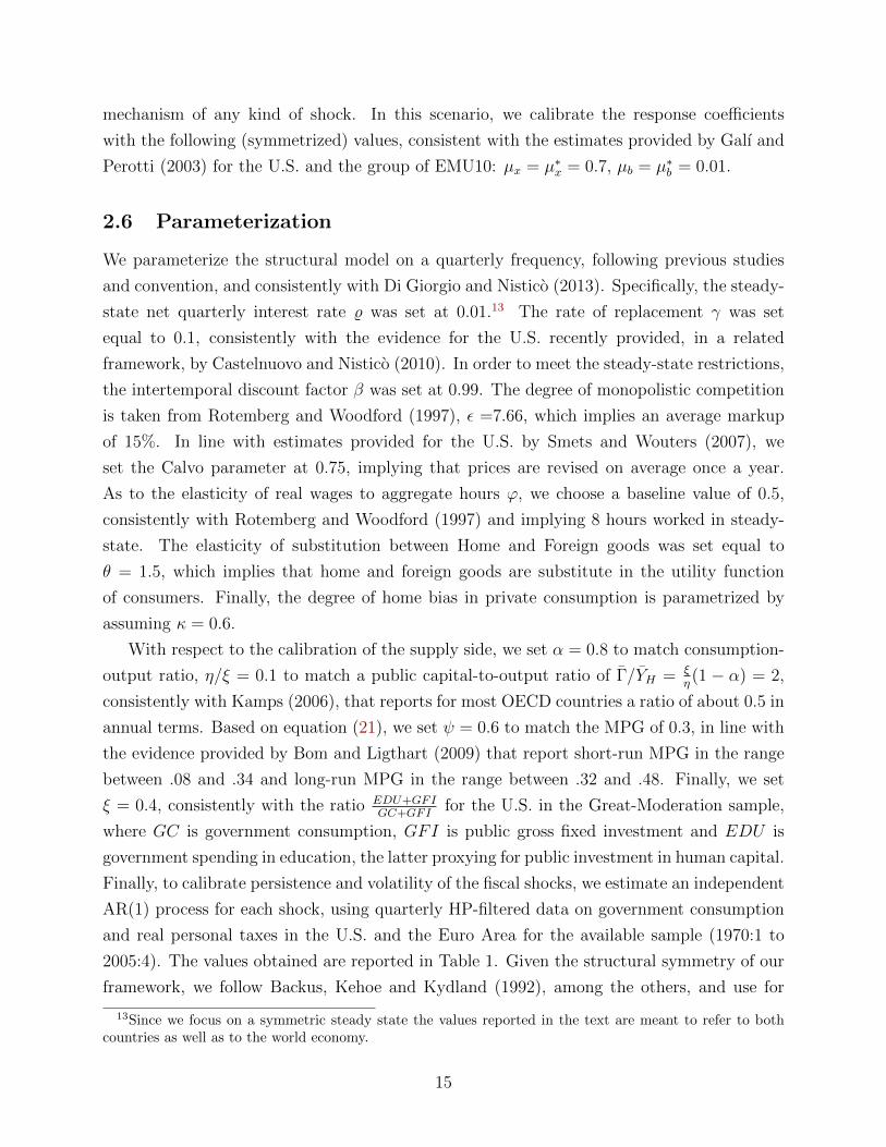
Figure 3: Balanced-budget increase in public spending: the role of home bias in public spending in thebenchmark NOEM model. Solid line: full home bias; dashed line: full diversification.
reaction. An increase in public spending that is directed towards both home and foreign
goods has positive effects on the marginal costs of both countries. However, since the fiscal
expansion is financed by an increase in domestic taxes only, relative consumption falls. As
a result, foreign marginal costs and inflation increase more than domestic ones, triggering
a relatively stronger response by foreign monetary policy. Contrary to the case of home-
biased public spending (solid line in figure 3), therefore, the relative interest rate falls and
the nominal and the real exchange rate depreciate.
Figure 4 extends this exercise to our model with productive government spending. The
real exchange rate depreciates regardless of the specific assumption on the degree of home
bias in public consumption. Notice that, in the case of full diversification (dashed line),
the increase in public spending increases marginal costs in both countries; however, since the
fiscal expansion only affects domestic labor productivity, relative marginal costs and inflation
are lower, triggering a fall in relative interest rates and a nominal and real depreciation. In
this case, the demand effect on domestic inflation is smaller in size since part of this expansion
falls on foreign goods. As a consequence, the on-impact depreciation is higher than in the
case of complete home bias, while the long run path is similar. While under the assumption
of home-biased public spending the nominal exchange rate remains depreciated throughout
the transition, in the case of full international diversification, it gradually converges to a
permanently appreciated level.
19

0 20 40-0.05
0
0.05
0.1
0.15 domestic output gap
0 20 40-0.05
0
0.05
0.1
0.15 domestic inflation
0 20 400
0.01
0.02
0.03
0.04
0.05
0.06 rer
0 20 40-1
-0.5
0
0.5
1 primary deficit
Full Home Bias
0 20 403.5
4
4.5
5 nom. interest rate H
0 20 40-0.2
-0.1
0
0.1
0.2
0.3
0.4 nom. exchange rate
Full Diversification
Figure 4: Balanced-budget increase in public spending: the role of home bias in public spending in themodel with productive public spending. Solid line: full home bias; dashed line: full diversification.
All the effects discussed so far are clearly independent of the overlapping-generation struc-
ture of our DNK model. The balanced-budget specification of the fiscal expansions considered
thus far does not allow to consider the accumulation of public debt and therefore the role
of wealth effects. Our overlapping-generation structure, however, allows us to go further
and evaluate whether the results obtained in the case of balanced-budget spending shocks
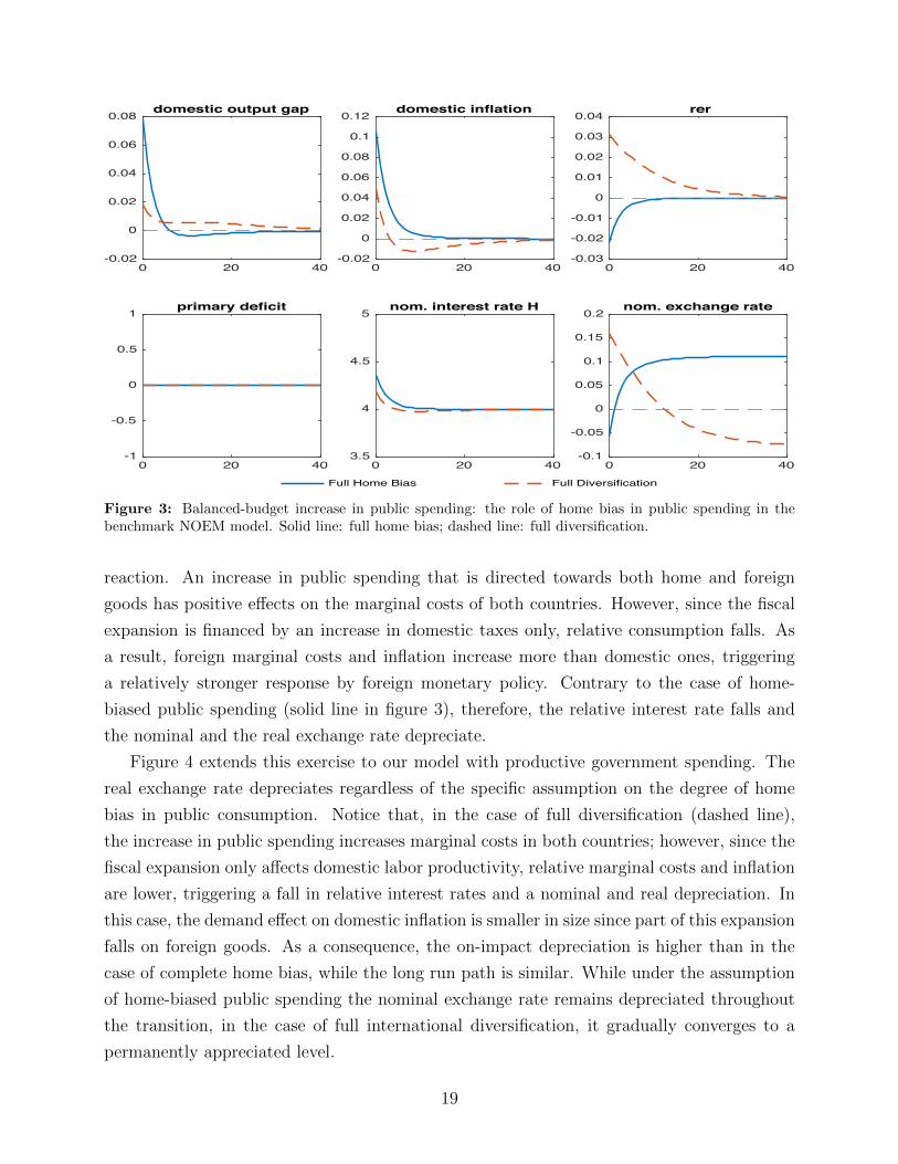
are robust to alternative assumptions about the financing of the latter. Figure 5 shows the
effects of an unbalanced increase in government spending under two different fiscal regimes:
an endogenous countercyclical fiscal policy (solid line), described by rule (50), and exogenous
fiscal policy (dashed line), where real taxes follow a stationary autoregressive process such
as (49). The simulation shows how the fiscal policy regime affects the on impact reaction of
the real exchange rate. The exchange rate depreciates under endogenous fiscal policy (more
intensively with respect to the balanced budget case displayed in Figure 1). Under an exoge-
nous tax rule, the government runs a significant primary deficit which amplifies the demand
effect of the fiscal shock. As a consequence, domestic inflation is much higher and the real
exchange rate appreciates on impact. Notice, however, that after the short-run appreciation,
the real exchange rate overshoots its long-run equilibrium level and remains depreciated
throughout the transition, as in the case of endogenous fiscal policy. In the medium run,
moreover, the real exchange rate depreciates even more when fiscal policy is exogenous, given
the accumulation of net foreign liabilities implied by the lack of fiscal discipline. The degree
20
0 20 40-0.05
0
0.05
0.1
0.15 domestic output gap
0 20 40-0.05
0
0.05
0.1
0.15
0.2
0.25
0.3 domestic inflation
0 20 40-0.03
-0.02
-0.01
0
0.01
0.02
0.03
0.04 real exchange rate
0 20 40-0.2
0
0.2
0.4
0.6
0.8
1
1.2 real taxes
Countercyclical Deficit Rule
0 20 40-0.5
0
0.5
1
1.5 primary deficit
0 20 403.5
4
4.5
5 domestic interest rate
Acyclical Fiscal Policy
Figure 5: Non balanced-budget increase in public spending: the role of endogenous countercyclical fiscalrules. Solid line: endogenous countercyclical fiscal policy; Dashed line: exogenous fiscal policy.
of fiscal discipline is another non-negligible dimension affecting the exchange-rate response to
public spending shocks. Figure 6 compares the exogenous fiscal regime of Figure 5 (dashed
line) with one in which the tax rule responds more aggressively to the level of public debt
(ξb = 0.1 in rule (49)): the real exchange rate depreciates also on impact, the more so the
more disciplined is fiscal policy towards public debt (see solid line in Figure 6).17
The previous investigation allows us to better understand the effects on the exchange rate
of different ways of financing public spending. In particular, the effects of a debt-financed
increase in public spending can be decomposed as the sum of a tax cut and a balanced-budget
expansion. Using a perpetual-youth version of the Redux model, Ganelli (2005b) found
that, while a balanced-budget expansion would imply a depreciation through a reduction in
relative consumption and an increase in domestic prices, a tax-cut tends to appreciate the
exchange rate on impact. As a consequence, the final effect on the exchange rate is ambiguous.
Our simulations overcome the ambiguity result of Ganelli (2005b). In our framework with
productive public capital, a debt-financed expansion in public consumption unambiguously
induces a real depreciation in the medium run. The real exchange rate depreciates on impact
17We also simulated the effect on an an expansionary fiscal policy conducted via a debt-financed tax cut,under alternative degrees of fiscal discipline. Clearly, in this case the expansionary effect of fiscal shock istransmitted only through the “demand-side channel”. Since it does not affect labor productivity, the tax cuttriggers a persistent exchange rate appreciation as in the standard NOEM models without public capital.The result holds independently of the specific degree of fiscal discipline.
21

0 20 40-0.05
0
0.05
0.1
0.15 domestic output gap
0 20 40-0.05
0
0.05
0.1
0.15
0.2
0.25
0.3 domestic inflation
0 20 40-0.03
-0.02
-0.01
0
0.01
0.02
0.03
0.04 real exchange rate
0 20 40-0.05
0
0.05
0.1
0.15
0.2
0.25
0.3 real taxes
Fiscal Discipline
0 20 40-0.5
0
0.5
1
1.5 primary deficit
0 20 403.5
4
4.5
5 domestic interest rate
No Fiscal Discipline
Figure 6: Debt-financed increase in public spending: the role of fiscal discipline. Solid line: exogenous fiscalpolicy with fiscal discipline; Dashed line: exogenous fiscal policy with no fiscal discipline.
when fiscal policy is “sufficiently” aggressive, as shown by Figure 5 and 6.
Overall, the results of this section suggest that the role played by government-spending
externality on labor productivity allows to reconcile the prediction of a general NOEM model
with the widespread evidence documenting a real exchange rate depreciation following an
expansionary fiscal policy.
4 Concluding Remarks
This paper provides a characterization of the effects of different fiscal shocks on the exchange
rate. We analyze both balanced-budget and debt financed fiscal expansions when govern-
ment spending positively affects labor productivity in the private sector. Consistently with
empirical evidence, the real exchange rate generally depreciates following an increase in pub-
lic spending – both on impact and in the transition – while in standard NOEM models the
same shock produces an exchange-rate appreciation. The mechanism we analyze is able to
offset the positive effect on marginal costs induced by higher domestic demand following an
increase in government purchases. In our model, a positive shock in public spending improves
private sector’s productivity: this lowers domestic real marginal costs and triggers a lower
interest rate response by the domestic monetary authority. Consequently, the real exchange
22

rate depreciates.
We also show that the short-run response of the exchange rate is, in general, affected
by public spending composition, the degree of endogeneity in monetary policy, and also the
overall fiscal regime (in terms of the degrees of counter-cyclicality and fiscal discipline) when
the spending shock is unbalanced. In particular, in the latter case, the real exchange rate
depreciates on impact if the government follows either a sufficiently countercyclical feedback
rule on the primary deficit or a tax rule with sufficiently high degree of fiscal discipline. In
all cases, however, we find a persistent depreciation in the medium run.
23

References
.
Aschauer, David A. (1989). “Is Public Expenditure Productive?”, Journal of Monetary
Economics, vol. 23, pp. 177–200.
Basu, Parantap and Robert Kollmann (2013). ““Productive Government Purchases and
the Real Exchange Rate”, The Manchester School, vol. 81(4), pp. 461–469.
Beetsma, Roel M. W. J. and Henrik Jensen. (2005) “Monetary and Fiscal Policy Interac-
tions in a Micro-founded Model of a Monetary Union”, Journal of International Economics
67, pp. 320–352.
Beetsma, Roel M. W. J., Frank Klasssen and Massimo Giuliodori (2008). “The Effects
of Public Spending Shocks on Trade Balances and Budget Deficits in the European Union”,
Journal of European Economic Association vol. 6, pp. 414–423.
Benetrix, Agustin and Philip R. Lane (2013). “Fiscal Shocks and the Real Exchange
Rate”, International Journal of Central Banking vol. 9(3), pp. 1–32.
Benigno, Pierpaolo. (2004). “Optimal Monetary Policy in a Currency Area”, Journal of
International Economics, Vol. 63, Issue 2, pp. 293–320.
Blanchard, Olivier J. (1985). “Debt, Deficits, and Finite Horizons”, Journal of Political
Economy, 93.
Bom, Pedro R.D. and Jenny Ligthart (2009). “How Productive is Public Capital? A
Meta-Regression Analysis”, International Center for Public Policy Working Paper Series.
Calvo, Guillermo. (1983) “Staggered Prices in a Utility Maximizing Framework”, Journal
of Monetary Policy, 12.
Card, David E. (1994). “Intertemporal Labor Supply: An Assessment”, in Chris Sims, ed.,
Advances in Econometrics, Sixth World Congress, New York: Cambridge University Press.
Castelnuovo, Efrem and Salvatore Nistico (2010). “Stock Market Conditions and Mon-
etary Policy in a DSGE Model for the U.S.”, Journal of Economic Dynamics and Control
vol.34(9), pp.1700–1731.
Cavallo, Michele and Fabio Ghironi (2002). “Net Foreign Assets and the Exchange Rate:
Redux Revived”, Journal of Monetary Economics, vol. 49(5), pp. 1057-1097.
Corsetti, Giancarlo and Paolo Pesenti (2001). “Welfare And Macroeconomic Interdepen-
dence”, The Quarterly Journal of Economics, vol. 116(2), pp. 421–445.
Corsetti, Giancarlo, Andre Meier and Gernot J. Muller (2012). “Twin Deficit or Twin
Divergence? Fiscal Policy, Current Account, and Real Exchange Rate in the US”, The Review
of Economics and Statistics vol. 94(4), pp 878–895.
Devereux, Michael and Charles Engel (2003). “Monetary Policy in the Open Economy
24

Revisited: Price Setting and Exchange-Rate Flexibility”, Review of Economic Studies, vol.
70, pp. 765–783.
Di Giorgio, Giorgio and Salvatore Nistico (2007). “Monetary Policy and Stock Prices in
an Open Economy”, Journal of Money Credit and Banking, 39, 8, pp. 1947–1985.
Di Giorgio, Giorgio and Salvatore Nistico (2013). “Productivity Shocks, Stabilization So-
licies and the Dynamics of Net Foreign Assets”, Journal of Economic Dynamics and Control,
37, 1, pp. 210–230.
Di Giorgio, Giorgio, Salvatore Nistico and Guido Traficante (2015). “Fiscal shocks and
the Exchange Rate in a Generalized Redux Model”, Economic Notes, 20, pp. 1–16.
Galı, Jordi, J. David Lopez-Salido and Javier Valles (2007). “Understanding the Effects
of Government Spending on Consumption”, Journal of the European Economic Association,
5, 1, pp.227–270.
Galı, Jordi and Tommaso Monacelli (2005). “Monetary Policy and Exchange Rate Volatil-
ity in a Small Open Economy”, Review of Economic Studies, 72, pp. 707-734.
Galı, Jordi and Roberto Perotti (2003). “Fiscal Policy and Monetary Integration in Eu-
rope”, Economic Policy, 37, pp. 533-572.
Ganelli, Giovanni (2005a). “Home Bias in Government Spending and Quasi Neutrality of
Fiscal Shocks”, Macroeconomic Dynamics, 9, pp. 288–294.
Ganelli, Giovanni (2005b). “The New Open Economy Macroeconomics of Government
Debt”, Journal of International Economics, 65, pp. 167-184.
Iwata, Yasuharu (2013). “Two fiscal policy puzzles revisited: New evidence and an expla-
nation”, Journal of International Money and Finance, 33, pp. 188-207.
Kamps, Christophe (2006). “New Estimates of Government Net Capital Stocks for 22
OECD Countries 1960-2001”, IMF Staff Papers, Palgrave Macmillan, 53(1), pp. 120-150.
Kim, Soyoung and Nouriel Roubini (2008). “Twin Deficit or Twin Divergence? Fiscal
Policy, Current Account, and Real Exchange Rate in the US”, Journal of International
Economics vol. 4, pp. 362–383.
Kollmann, Robert (2010). “Government Purchases and the Real Exchange Rate”, Open
Economies Review, vol. 21, pp. 49–64.
Leith, Campbell and Leopold von Thadden (2008). “Monetary and fiscal policy interac-
tions in a New Keynesian model with capital accumulation and non-Ricardian consumers”,
Journal of Economic Theory
Leeper, E. M. (1991). “Equilibria Under ’Active’ and ’Passive’ Monetary and Fiscal
Policies”, Journal of Monetary Economics 27, pp. 129-47.
Monacelli, Tommaso and Roberto Perotti (2010). “Fiscal Policy, the Real Exchange Rate
and Traded Goods”, The Economic Journal vol. 120, pp. 437–461.
25

Nistico, Salvatore (2014). “Optimal Monetary Policy and Financial Stability in a non-
Ricardian Economy”, DISSE Working Paper n.6/2014, forthcoming in the Journal of the
European Economic Association
Nistico, Salvatore (2012). “Monetary Policy and Stock-Price Dynamics in a DSGE Frame-
work.” Journal of Macroeconomics, vol. 34 (1), pp. 126–146.
Obstfeld, Maurice and Kenneth S. Rogoff (1995). “Exchange Rate Dynamics Redux.”
Journal of Political Economy, 103, 624-60.
Rotemberg, Julio and Micheal Woodford (1997). “An optimization-based econometric
framework for the evaluation of monetary policy”, In: Bernanke, B., Rotemberg, J. (Eds.),
NBER Macroeconomics Annual 1997, MIT Press, Cambridge.
Smets, Frank and Raf Wouters (2003). “An estimated dynamic stochastic general equi-
librium model of the Euro area”, Journal of the European Economic Association, vol. 1, pp.
1123–1175.
Smets, Frank and Raf Wouters (2007). “Shocks and frictions in US business cycles: a
Bayesian DSGE approach”, American Economic Review, vol 97, pp. 586–606.
Schmitt-Grohe, Stephanie and Martin Uribe (2007). “Optimal Simple and Implementable
Monetary and Fiscal Rules”, Journal of Monetary Economics, vol. 54, pp. 1702–1725.
Taylor, John B. (1993). “Discretion versus Policy Rules in Practice”, Carnegie-Rochester
Conference Series on Public Policy, 39.
Yaari, Menahem E. (1965). “Uncertain Lifetime, Life Insurance, and the Theory of the
Consumer”, Review of Economic Studies, 32.
26

Appendix
A The Complete Model
At time t, the complete set of conditions needed to study the international equilibrium are:
1. labor-supply schedules, both countries
δCt = Wt(1− Lt) (51)
δC∗t = W ∗t (1− L∗t ) (52)
2. private-sector budget constraints, aggregate per-capita terms, both countries
Ct + EtFt,t+1Ωt = WtLt +Dt − Tt +Ωt−1
1 + πt(53)
C∗t + EtF∗t,t+1Ω∗t = W ∗t L∗t +D∗t − T ∗t +
Ω∗t−1
1 + π∗t(54)
3. dynamic equations for aggregate consumption, both countries
Ct = σEtFt,t+1Ωt +1
βEt Ft,t+1(1 + πt+1)Ct+1 (55)
C∗t = σEtF∗t,t+1Ω∗t +1
βEtF∗t,t+1(1 + π∗t+1)C∗t+1
(56)
4. relative prices, both countries
PH,tPt
=[κ+ (1− κ)S1−θ
t
] 1θ−1 ≡ h(St) (57)
P ∗F,tP ∗t
=[κ+ (1− κ)Sθ−1
t
] 1θ−1 ≡ f(St) (58)
Where St denotes the terms of trade:
St ≡PF,tPH,t
=P ∗F,tP ∗H,t
5. demand for domestic goods, both sectors and both countries
YH,t = κ
(PH,tPt
)−θCt + (1− κ)Sθt
(P ∗F,tP ∗t
)−θC∗t +Gt (59)
Y ∗F,t = (1− κ)S−θt(PH,tPt
)−θCt + κ
(P ∗F,tP ∗t
)−θC∗t +G∗t (60)
27

6. public-sector budget constraints, per-capita terms, both countries
Bt =1 + rt−1
1 + πtBt−1 + Zt, (61)
B∗t =1 + r∗t−1
1 + π∗tB∗t−1 + Z∗t , (62)
Zt =PH,tPt
Gt − Tt (63)
Z∗t =P ∗F,tP ∗t
G∗t − T ∗t (64)
7. real marginal costs, both countries
MCt =Wt
Γψt
PtPH,t
(65)
MC∗t =W ∗t
Γ∗ψt
P ∗tP ∗F,t
(66)
8. aggregate production functions, both sectors and both countries
ΞtYH,t = Γψt Lt (67)
Ξ∗tY∗F,t = Γ∗ψt L∗t (68)
9. aggregate dividends, economy-wide, both countries
Dt =PH,tPt
YH,t −WtLt (69)
D∗t =P ∗F,tP ∗t
Y ∗F,t −W ∗t L∗t (70)
10. Uncovered Interest Parity
Et
Ft,t+1
[Et+1
Et(1 + r∗t )− (1 + rt)
]= 0 (71)
11. optimal consumer-price setting equations, both countries
Et
∞∑k=0
ϑkFt,t+kYH,t+kP εH,t+k
[P oH,t − (1 + µ)MCt+kPH,t+k
]= 0 (72)
Et
∞∑k=0
ϑkF∗t,t+kY ∗F,t+kP ∗εF,t+k
[P ∗oF,t − (1 + µ)MC∗t+kP
∗F,t+k
]= 0 (73)
Moreover, the following definitions hold:
NFAt ≡ Ωt −Bt = −QtNFA∗t Qt ≡EtP ∗tPt
=h(St)f(St)
St
CAt ≡ NFAt −NFAt−1
1 + πt
28

B The Steady-State.
In this Section we derive the relations characterizing a zero-inflation, zero-deficit symmetric steady state. In
such steady state we have, by assumption, G = G∗ and Z = Z∗ = 0. Moreover, MC = MC∗
= (1 + µ)−1
and Γ = Γ∗.
This further implies B = B∗ = Ω = Ω∗ = 0 and S = Q = 1. The Uncovered Interest Parity implies
r = r∗. The latter, together with equations (9)–(10), implies r = (1− β)/β and C = C∗.
Equations (59) and (60) imply:
C + G = YH = Y ∗F .
Equilibrium marginal costs, labor supplies and production functions in each country further imply (given
structural symmetry):
YH =Γψ + δ(1 + µ)G
1 + δ(1 + µ)
C =Γψ − G
1 + δ(1 + µ)
L =1 + δ(1 + µ)GΓ−ψ
1 + δ(1 + µ)
W =Γψ
1 + µ.
Notice that the non-negativity constraint on consumption implies the following restriction on the parameters
governing the dynamics of public capital:
Γψ > G.
From the above, the following two composite parameters derive
ϕ ≡ L
1− L=
1 + δ(1 + µ)GΓ−ψ
δ(1 + µ)(1− GΓ−ψ)(74)
α ≡ C
YH=C∗
Y ∗F=
1− GΓ−ψ
1 + δ(1 + µ)GΓ−ψ, (75)
which are related to each other through
1 = αδ(1 + µ)ϕ. (76)
C The Flexible-Price Balanced-Budget Equilibrium (FBE)
Following Di Giorgio and Nistico (2013), we take as our benchmark the global allocation arising in the
absence of all distortions: the Flexible-price Balanced-budget Equilibrium (FBE). The “flexible-price” feature
of the FBE rules out the distortions due to monopolistic competition and nominal rigidities, to a first-order
approximation. The “zero-deficit” (balanced-budget) feature instead sterilizes – at the world level – the
third distortion due to the consumption dispersion across agents: since it implies a zero-stock of global
financial wealth, the dynamics of global consumption is undistorted. In the Flexible-price Balanced-budget
Equilibrium, therefore, the global fluctuations induced by structural shocks reflect the efficient dynamic
response of the economy.
29

In the FBE, marginal costs in both countries are equal to their steady state level at all times. Let mt
denote the level of generic variable mt in the FBE at time t, the relevant system of linear equations therefore
becomes:
qt = (2κ− 1)st (77)
0 =1
αcRt + ϕyRt + 2(1− κ)st − ψ
η(1 + ϕ)
ξ(1− α)(γt − γ∗t ) (78)
yH,t = 2αθκ(1− κ)st + κct + (1− κ)c∗t + gt (79)
y∗F,t = −2αθκ(1− κ)st + κc∗t + (1− κ)ct + g∗t (80)
0 =1
α(ct + c∗t ) + ϕ
(yH,t + y∗F,t
)− ψη(1 + ϕ)
ξ(1− α)(γt + γ∗t ) (81)
cRt = EtcRt+1 − αEt∆qt+1 + 2σnfat + σb
R
t (82)
nfat =1
βnfat−1 +
1
2
(yRt − gRt − cRt
)− α(1− κ)st (83)
bt = β−1bt−1 + zt (84)
b∗t = β−1b
∗t−1 + z∗t (85)
zt = gt − τ t − (1− α)(1− κ)st (86)
z∗t = g∗t − τ∗t + (1− α)(1− κ)st (87)
γt = (1− η)γt−1 + ξgt (88)
γ∗t = (1− η)γ∗t−1 + ξg∗t (89)
yRt = yt − y∗t (90)
cRt = ct − c∗t (91)
gRt = gt − g∗t (92)
bR
t = bt − b∗t (93)
zt =β − 1
βbt−1 (94)
z∗t =β − 1
βb∗t−1 (95)
The last two equations in the system above define the fiscal rules that implement the FBE and guarantee
that the levels of home and foreign real debt are stabilized at their initial levels: b−1 = 0 and b∗−1 = 0.
Specifying some initial conditions also for the net foreign asset position and relative prices (nfa−1 = 0, and
s−1 = 0), the above system of 19 stochastic difference equations delivers as a solution the equilibrium values
of the 19 endogenous variables:
γt, γ∗t , qt, st,nfat, bt, b∗t , ct, c
∗t , c
Rt , g
Rt , yH,t, y
∗F,t, y
Rt , b
R
t , zt, z∗t , τ t, τ
∗t ∞t=0
30