Government policy and the dynamics of market

structure: Evidence from Critical Access Hospitals

Gautam Gowrisankaran∗ Claudio Lucarelli† Philipp Schmidt-Dengler‡

Robert Town§

April 27, 2009

Very Preliminary and Obviously Incomplete – Please Do Not Cite

Abstract

This paper seeks to understand the impact of the Medicare Rural Hospital FlexibilityProgram. The overarching goal of this legislation is to maintain access to qualityhospital care for rural residents. To achieve this objective, the program created anew class of hospital, the Critical Access Hospital (CAH), to which rural hospitals canconvert. Like many other government policies, the CAH program targets the underlyingsupply infrastructure, in this case by providing generous cost-plus reimbursement toconverting hospitals in exchange for capacity and service limitations. We specify adynamic oligopoly model of the rural hospital industry with hospital investment incapacity, exit and conversion to CAH status. We develop new methods that allow usto estimate the structural parameters efficiently and compute counterfactual equilibria.We use the methods to estimate the impact of eliminating and modifying the CAHprogram on access to hospitals and patient welfare. Our methods may be more broadlyuseful in estimating and computing other dynamic oligopoly games with investment incapacity.

Keywords: Hospitals, Exits, Dynamic Oligopoly, Medicare. JEL Classification: L11, L13,

L31, L38, I11, I18

∗University of Arizona and NBER†Cornell University‡London School of Economics and OeNB§University of Minnesota and NBER

1 Introduction

As part of the Budget Balance Act of 1997, the Congress passed and the President signed

the Medicare Rural Hospital Flexibility Program. The overarching goal of this legislation is

to maintain access to quality hospital care for rural residents. To achieve this objective, the

program created a new class of hospital, the Critical Access Hospital (CAH), to which rural

hospitals can convert. This paper seeks to understand the impact of this program on the

rural hospital infrastructure by estimating a dynamic oligopoly model of the rural hospital

industry. The paper has two interrelated objectives. First, we aim to quantify the impact

of this important policy which coincided with and likely caused large effects on the supply

infrastructure of rural healthcare delivery. Second, we develop methods to compute dynamic

oligopoly models of capacity games that may be useful for other industrial organization

questions and that allow us to compare the efficiency of recently developed methods for

estimating dynamic oligopoly models.

The policy strategy embodied in the CAH program is not unique to this specific interven-

tion as many other government policies seek to achieve their goals by targeting the underly-

ing supply infrastructure. Examples abound and span countries and industries. Agricultural

price supports impact the number and size distributions of farms. Education vouchers and

the Charter school option affect the number and size distribution of private schools. Given

the magnitude of these supports the welfare consequences of these programs are likely large.

As these programs affect the returns to market participation, their impact is an indirect

consequence of their effect on entry, exit and investment decisions by a potentially large

number of market participants. The decisions by market participants in turn are typically

generated by the equilibrium of a dynamic game whose payoffs vary with policy changes. For

this reason, assessing the impact of these programs on welfare and other outcomes is often a

difficult task, requiring solving and estimating dynamic oligopoly models.

In this paper we seek to understand the impact of the CAH program on the U.S. rural

hospital infrastructure and societal welfare.1 The overarching purpose of this program is

1For expositional ease we refer to the Medicare Rural Hospital Flexibility Program as the CAH program.

2

to improve the access to care of the rural population by keeping open hospitals that would

otherwise close and to provide additional resources to hospitals to improve the quality of care.

The CAH initiative is a voluntary program in which participating hospitals comply with a

number of restrictions, principally, limits on their capacity to 25 beds or less and limits on

services and length-of-stay to proscribed levels. In return for participating, hospitals opt out

of the standard Prospective Payment System (PPS) and receive cost-based reimbursements

from the Medicare program. These payments are generally significantly more generous than

what the hospital would earn under PPS. Since the implementation of the program, over 1,200

rural hospitals (roughly 25% of all US hospitals) have converted to CAH status. CAH status

also coincided with a dramatic reduction in the capacity of rural hospitals: in 1997, 15% of

rural hospitals had 25 beds or less, while that figure rose to 45% by 2004. In 2006, government

estimates find that CAH hospitals received $5 billion in cost-based reimbursements, $1.3

billion more than what they would have received under PPS (MedPAC 2005).

The large scale of the CAH program, its costliness and the subsequent change in hospital

market structure all suggest that an evaluation of the consequences of the CAH program is

important. Specifically, an evaluation can inform us about the impact of the CAH program

on rural hospital infrastructure and alternate counterfactual policy programs on welfare and

industry structure.

To evaluate the impact of the CAH program, we specify a dynamic model of rural hos-

pital exit, investment and CAH status.2 Each period, hospitals endogenously select their

investment or disinvestment in beds, decide whether to exit and post-1997 select whether

or not to invest in converting to a CAH. Prior to making its investment decision, each firm

obtains a private information shock to its capacity investment cost. We allow for non-linear

adjustment costs in beds and a stochastic outcome to the CAH investment decision. The

private information shock and stochastic CAH outcome generate randomness in the outcomes

of the model, necessary both for the existence of pure strategy equilibria and a well-defined

likelihood function. Following the hospital decisions, in each period, with some probability,

individuals fall ill and decide at which hospital to seek treatment. Hospitals earn revenue and

2Entry is rare in rural hospital markets and therefore our analysis does not consider it.

3

incur costs from treating patients that are admitted to their facility.3 They seek to maximize

an objective function that includes profits, volume and the provision of service, in the case of

not-for-profit (NFP) and government hospitals. The decisions are made in a Markov Perfect

equilibrium, where hospitals take account of the effect of their investment and conversion

decisions on other hospitals in their market. Our model is a function of unknown parameters

that pertain to the objective functions for NFP and government hospitals, the cost function

for investing or disinvesting in capacity and exit, the costs of obtaining CAH status and the

size of the random cost shock.

One could estimate the policy impact of the CAH program by evaluating the role that

exposure to the CAH program had in affecting changes in industry structure using reduced-

form regressions of hospital exit and investment on exposure to the CAH program. This

potential approach has two important limitations. First, as is well-known, such a reduced-

form estimation can at most be used to derive the impact of the CAH program on hospital exit

or capacity and cannot be used to understand the welfare implications of this policy or the

impact of counterfactual CAH policies. Second, and perhaps less appreciated, the structural

estimation has much more transparent and less demanding identification. This is because the

structure imposed by our model allows us to identify only structural parameters rather than

more complicated equilibrium policy responses. Specifically, the reduced-form regressions

above would have to include regressors to capture current and future information about the

hospital and all its competitors, and interactions of these variables with the CAH legislation.

In contrast, our structural approach has relatively few structural parameters to identify

but then it aggregates them into industry and welfare impacts using a dynamic oligopoly

structure. Moreover, it is straightforward to understand how these structural parameters are

identified. For instance, the cost of investment in beds or CAH status are identified by the

extent to which gross profits change following the change in state variables relative to the

likelihood of choosing that policy. Thus, if CAH status increases profits for certain hospitals

significantly but those hospitals rarely convert our model infers that conversion is very costly.

3A companion paper (in process), analyzes the static patient choice model for rural hospital patients and

the determinants of static profits for hospitals.

4

Thus, we proceed by estimating the parameters of the dynamic oligopoly model. A

number of recent papers have developed methods to estimate the parameters of such models.

The idea behind these methods was first developed by Hotz and Miller (1993) in the context

of dynamic single-agent models with discrete choices. Hotz and Miller (1993)’s insight is

that future observed strategies can be used in place of optimizing behavior, thereby averting

the computational burden of solving for the dynamic decision problem when estimating the

structural parameters of the model. This insight was extended to dynamic oligopoly models

with many or continuous choices by Bajari et al. (2007) (henceforth BBL).4 BBL extend

the original Hotz and Miller (1993) idea to compare the observed choices against a menu

of counterfactual policies and the transition matrix implied by the data. This effectively

eliminates both the need to compute dynamic oligopoly behavior and even to solve for optimal

policies given other firms’ actions and thereby reduces computation time.

There are two issues with using the BBL method in our context. First, they do not provide

a method for computing the equilibrium of the model and this computation is necessary to

compute the impact of counterfactual policies. Second, while BBL reduces computation

time, it does so at the cost of a higher requirement on the data and a potentially large loss

in efficiency. Specifically, with BBL, the data must be sufficiently rich to estimate accurately

the dynamic transition matrix and the set of alternative policies must be sufficiently broad

to identify the structural parameters.

These concerns suggest that it is necessary to compute the dynamic oligopoly directly.

Dynamic oligopoly models that are most frequently computed are based on the Pakes and

McGuire (1994) model and specify quality ladder games with a stochastic and discrete, typi-

cally binary, investment realization. These models are not designed for capacity accumulation

games such as ours.5

We develop new methods to compute dynamic oligopoly models for capacity games where

firms have private information and choose their new level of capacity given their information.

4Pakes et al. (2007), Aguirregabiria and Mira (2007) and Pesendorfer and Schmidt-Dengler (2007) have

also suggested approaches to estimate parameters of dynamic games.5These models also do not have any private information and hence do not generate a well-defined likelihood.

5

A standard approach to computing a monopoly capacity model is to choose a finite number

of grid points and solve the optimal policy for these grid points. This approach runs into

difficulties when analyzing multiple firms as the finite approximation model may not have

a pure strategy equilibrium even when the limiting game has such an equilibrium. This is

because the reaction functions are no longer continuous. Our approach differs by deriveing

the exact cutoff points between different values of investment. Specifically, using the su-

permodularity of our investment decision, we show that the capacity decisions that will be

chosen with positive probability are those which lie on a discrete analog of a convex hull of

the choice-specific value function, defined as the value function conditional on any capac-

ity decision. We use this result to derive an algorithm that iteratively discards investment

levels that are not in the discrete convex hull and then solves for the exact cutoff values of

the private information shocks that result in indifference between any two remaining invest-

ment levels. By calculating the exact probability of each investment decision, pure-strategy

equilibrium for our model exists and is relatively easily computable.

We use our equilibrium computation method in three ways. First, we estimate the param-

eters of the model using maximum likelihood. This estimation is limited to markets with one

or two firms as markets with more than two firms is too computationally intensive. Second,

we modify the BBL method: while BBL compare the observed policy to a selected set of

alternative policies, we solve for the optimal policy given any vector of structural parame-

ters and then use this to derive the quasi-likelihood of the observed policy and estimate the

parameters using likelihood methods. We expect that this modification will vastly increase

the efficiency of the method. Finally, we use it to derive the equilibria corresponding to

counterfactual policies. Our counterfactual policies include having no CAH program, having

different hospital size thresholds and changing the CAH policy to a lump-sum transfer.

The remainder of this paper is divided as follows. Section 2 provides the institutional

background of the CAH program. Section 3 describes our data. Our model is presented in

section 4, and section 4.1 describes our estimation method. The results and policy experi-

ments are presented in sections 5 and 6 respectively, and section 7 concludes.

6

2 The Critical Access Hospital Program

2.1 Background

The CAH program was enacted in the Balanced Budget Act (BBA) of 1997.6 Desig-

nated CAHs receive cost-based Medicare reimbursements for inpatient, outpatient post-acute

(swing bed) and laboratory services. To qualify for the program, hospitals must be 35 miles

from a primary road and 15 miles by a secondary road to the nearest hospital. However, this

distance requirement can be waived if the hospital is declared a “necessary provider” by the

state, and, until 2006, the distance requirement does not appear to be binding. Most CAHs

are less than 25 miles from a neighboring hospital. The BBA legislation stated that CAHs

can only treat 15 acute inpatients and 25 total patients including patients in swing beds. A

swing bed is one which can be used to provide either acute or skilled nursing facility care.

The 1997 legislation set the maximum hospital size to 15 beds and the length of stay for any

patient was limited to 4 days.

CAH hospitals are required to provide inpatient, laboratory, emergency care and radiology

services. A CAH must also develop agreements with an acute care hospital related to patient

referral and transfer, communication, emergency and non-emergency patient transportation.

The CAH may also have an agreement with their referral hospital for quality improvement

or choose to have that agreement with another organization. Lastly, the CAH legislation

provides resources for hospitals to hire consultants to project revenues and costs under the

CAH program and determine which strategy is best for the hospital given their objectives.

The program’s rules have been modified several times since its inception. Table 1 sum-

marizes the important legislative and regulatory changes in the program. The most impor-

tant of these changes likely are: 1) The Balanced Budget Reconciliation Act (BBRA) of

1999 changed the length of stay requirement and allowed states to designate hospitals in

Metropolitan Statistical Areas ‘rural’ for CAH classification; 2) The Medicare Prescription

Drug, Improvement and Modernization Act (MMA) of 2003 increased the acute inpatient

6Much of the information in the section is culled from MedPAC (2005), which contains much more back-

ground that we provide.

7

limit from 15 to 25 acute patients and increased the payments from 100 to 101 percent of

costs. Thus, there is variation in payoffs to becoming a CAH across both time and hospitals.

Figure 2 shows the rate of CAH conversion among all general acute care hospitals in

the U.S. Conversion rates were very low until 1999. Starting in 1999, there is roughly a

4% conversion rate per year until the end of our sample period. The delay between the

enactment of BBA in 1997 and the timing of conversion is likely due to the application

process, which requires large amount of paperwork, the timing of inspections necessary for

Centers for Medicare and Medicaid Services (CMS) approval and some uncertainty regarding

the administration of the program.For example, in the state of Wisconsin, the application

process is an 18-step process, detailed at http://www.worh.org/pdf etc/AppFlowChart.pdf

By 2005, 25% of candidate hospitals have adopted CAH. After 2006, when the minimum

distance requirement was enforced, the number of CAH conversions declined precipitously

(MedPAC 2005).

The spatial distribution of CAHs is shown in Figure 1. CAHs are present in most states,

except New Jersey, Delaware, Rhode Island, Connecticut, and Massachusetts, which do not

participate in the program. CAHs concentrate in the Midwest, and are mostly outside of

MSAs.

The CAH program affects the incentives of hospitals and patients along a number of

dimensions. These different incentives may have opposing impacts on welfare and thus the

aggregate welfare effects of the program are not obvious. The program affects the size of

rural hospitals as well potentially impacting exit probabilities, keeping open hospitals that

would otherwise close. Residents of rural areas may benefit from from the reduction in exit

because they would have to travel longer distances to receive medical care had the closest

hospital exited the market. This is indeed one of the purposes of the program. However,

insofar has hospital size is valued because of its direct and indirect relationship to the the

scope and quality of services provided by the hospital, the CAH program may reduce patient

welfare. In addition, impact of the CAH program on hospital prices for private pay patients

is unclear and the program is estimated to have increased Medicare expenditures. Finally,

the program lowers the incentives of hospitals to minimize costs and may interfere with the

8

evolutionary improvement of the industry trapping capital and utilizing resources that would

generate higher value elsewhere Jovanovic (1982).

2.2 Previous Research on Dynamics of Hospitals

A number of studies examine the exit behavior of hospital in a reduced form framework and

thus relate to the CAH program. For example, Lillie-Blanton et al. (1992) and Ciliberto

and Lindrooth (2007), find that smaller hospitals are more likely to close. Wedig et al.

(1989) finds that for-profit hospitals are more likely to exit due to competing uses of capital.

Similar conclusions are reached by Ciliberto and Lindrooth (2007) and Succi et al. (1997).

Hansmann et al. (2002) consider four types of ownership and they also find that for-profit

hospitals were the most responsive to reductions in demand by exiting the market, followed

by public nonprofits, religiously affiliated nonprofits, and secular nonprofits responded the

least. These papers have studied what determines exits, without taking into account strategic

interactions, as our work does.

With respect to the effect of closures on surviving hospitals, Lindrooth et al. (2003)

focused on urban hospitals and found that the costs per adjusted admission declined by

2-4% for all patients and by 6-8% for patients who would have been treated at the closed

hospital. They abstract from the issues of access to care that closures generate due to their

focus on urban hospitals within 5 miles from the closing one. In contrast, McNamara (1999),

studies the impact of rural hospitals closures on consumers’ surplus using a discrete choice

travel-cost demand model. He finds that the average compensating variation for the closure

of the nearest rural hospital that makes the average shortest distance increase from 9 miles

to 25 miles is about $19,500 dollars of 1988 per sample hospitalization. These papers all

consider the period before 1998, before hospitals were effectively converting into CAH.

Several more recent studies examine aspects of the CAH program. Stensland et al. (2003)

studies the financial effects of CAH conversion. Comparing hospitals that converted in 1999

to other small rural hospitals, they find a significant association of CAH conversion with

increases in Medicare revenue, increases in hospital profit margins from -4.1% to 1.0%, and

9

increases in costs per discharge of 17%. They state that local patients and CAH employees

benefit from the improved financial conditions, but do not calculate whether the benefits

are worth their cost. Stensland et al. (2004) redo their analysis for hospitals converting in

1999 and 2000, reaching similar conclusions. Casey and Moscovice (2004) studies the quality

improvement initiatives of two CAHs after conversion, and conclude that the cost-based

payments help the hospitals to fund activities that would improve quality of care such as

additional staff, staff training and new medical equipment.

Although this literature has enhanced our understanding of hospital exits and the CAH

program, it does not explicitly examine the welfare impact of the CAH program. Further-

more, this literature does not take into account the strategic interactions between hospitals.

Thus, it cannot be used to analyze the impact of CAH and of counterfactual policies for rural

hospitals.

A previous paper, ? developed an empirical framework to estimate structural parameters

from dynamic oligopoly model of the hospital industry. That paper focused on the impact

of the prospective payment system (among other policy counterfactuals) on hospital market

structure and welfare. In comparison to the previous paper, our current work incorporates

a much richer model of the hospital sector that allows for variation in geography, size and

hospital characteristics. Also, the current model is also more cleanly identified as we have

assembled a richer panel data set.

3 Data

We construct our dataset by by pooling and merging information from various sources. Pri-

marily, we use the publicly available Hospitals Cost Reports Information System (HCRIS)

panel data set from CMS for the years 1994-2005. Hospitals are required to file a cost report

at the end of each fiscal year, where they report detailed financial and operational informa-

tion needed to determine Medicare reimbursements, and this dataset contains the resulting

information. For our purposes, these data report the number of beds, inpatient discharges,

inpatient and outpatient revenues, salaries, and accounting information such as inpatient and

10

outpatient costs, depreciation, asset values and profits, as well as a unique provider number

assigned by CMS.7 Our HCRIS sample is the set of non-federal general acute care hospitals.

The information from the HCRIS was complemented with data on the timing of conversion

to CAH from the Flex Monitoring Team (Flex).8 When hospitals convert to CAH, a new

provider number is issued by CMS, even if ownership does not change, thus tracking hospitals

has they convert is a data challenge. By using the Flex data, we were able to link the new

and old provider numbers, which is necessary to understand the dynamics of the industry.

Using the merged data, we find that only 14 hospitals entered a particular market as a new

facility, and therefore, we do not model entry. In addition, the Flex data contains accurate

information on the number of beds for the hospitals that converted, which was used to verify

the HCRIS information.

We link these two datasets with the American Hospital Association Annual Survey (AHA),

using the CMS provider number to perform the linkage. Our primary use of the AHA data

is to determine hospital latitude and longitude which we use to compute distances between

patients and hospitals and to identify a hospital’s competitors.

We complete our hospital data with information from the Department of Health and

Human Services’ Office of Inspector General’s (OIG) reports on hospital closures, years 1994-

2000. These reports contain a list of the hospitals that exited the market during the year.

Because the year of exit in the OIG reports differs to the last report filed for about a third of

the exitors, we use the OIG information to identify exitors and we assume the hospital exits

at the end of the year of their last report. After 2000 we proceed in the same fashion, but

our source of data to identify closures are the Registered Deletions section from the AHA

Survey, years 2001 to 2005.

7The reporting periods for hospitals differs in length, and beginning and end dates. We created a panel

with one observation per calendar year, by disaggregating the data to the quarter level and then aggregated

it back to the calendar year level.8The Flex Monitoring Team is a collaborative effort of the Rural Health Centers at the Universities of

Minnesota, North Carolina and Southern Maine, under contract with the Office of Rural Health Policy. The

Flex Monitoring Team monitors the performance of the Medicare Rural Hospital Flexibility Program (Flex

Program), with one of its objectives being the improvement of the financial performance of CAH.

11

We rely on two data sources in order to construct measures of hospital inpatient flows by

payer class. From the CMS, we use the Health Services Area File which contains Medicare

hospital level discharge information by Medicare beneficiary ZIP code and year. We also

use data from the 2000 U.S. census under 65 year old population. This data is used to

roughly capture the geographic distribution of the non-Medicare population. We restrict our

attention to the population that is above the poverty line as the margins for treating those

patients with low income is low (if they are on Medicaid) or negative (if they are uninsured).

For our purposes, these data provide information on the number of people by age in each

census ZIP code.

Using the hospital data, we designate a set of hospitals that we determine are candidates

for CAH conversion. Because the policy’s stated objective is to maintain access to emergency

and inpatient care for rural residents we let rurality be a necessary condition for conversion.

We characterize rurality using the Rural-Urban Commuting Area Codes (RUCA), version

2.0.9 This measure is based on the size of cities and towns and their functional relationships

as identified by work commuting flows, and have been used by CMS to target other rural

policies, such as the ambulance payments. CMS considers a census tract to be rural if and

only if it has a RUCA greater or equal than 4, and we adopt the same criterion in this

paper.10 The definitions of the RUCAs are shown in Table 2. Since only small hospitals ever

convert to CAH status, we also allow only hospitals with 225 beds or less to be candidates

for CAH conversion. These two criteria determine our sample for ‘at-risk’ hospitals.

We then use the location data to determine geographic markets. We first define a 150 km

circle about the hospital. All hospitals in this circle, including those that are not candidates

for CAH conversion, are included in the market. Hospitals that are further away have a lesser

strategic impact than nearby hospitals.

9These measures are developed collaboratively by the Health Resources and Service Administration, the

Office of Rural Health Policy, the Department of Agriculture’s Economic Research Service, and the WWAMI

Rural Health Research Center.10Department of Health and Human Services, Medicare Program, Revisions to Payment Policies, etc.; Final

Rule. Dec 2006.

12

4 Model, computation and estimation

4.1 Model

We specify a dynamic oligopoly model where the strategic players are all hospitals with 225

beds or less in 1997 located in a zip code with a RUCA of four or higher.11 A market in our

model corresponds to a mutually exclusive geographic area where all players are within 50

KM of other players in the market but not within 50 KM of any player outside the market.

Denote the players in a market 1, . . . , J . Players are differentiated by their location,

CAH status, capacity (measured by beds), ownership type ownj and productivity. Time is

discrete with a period corresponding to a year and hospitals discount the future with the

same discount factor β.

Each period, we model a game with three stages. First, nature moves and provides each

hospital with a period-specific investment cost shock. Second, knowing the value of their

individual shocks – but not of other hospitals’ shocks – players in the market simultaneously

choose investment strategies for capacity, exit and CAH status. Finally, a static production

game occurs where each patient makes a discrete choice among available hospitals. While

we allow a hospital to change its capacity and CAH status, we assume that its other charac-

teristics are fixed. Denote the industry characteristics that are fixed within a market Ω and

denote the capacity and CAH status of each hospital in the market Ω. Since Ω is invariant,

we suppress it below to economize on notation. The environment for hospital j can thus be

written as (Ω, j).

Hospitals choose actions in order to maximize the expected discounted values of their net

future returns where returns depend on ownj. We model three ownership types: for-profit

(FP), not-for-profit (NFP) and government (Gov). For a FP hospital, returns in any period

are synonymous with profits, while for NFP and government hospitals, returns are a weighted

11We choose this limit for the set of strategic players because large or urban hospitals would be unlikely

to qualify for CAH status and likely do not make their decisions in response to small rural hospitals located

in an area around them.

13

sum of profits, patient volume and the provision of service.12 For NFP hospitals, we let the

weights on volume and the provision of service be denoted αNFPv and αNFP

p respectively; for

government hospitals we use αGovv and αGov

p , where the α values are parameters to estimate.

We normalize the weights on expected net profits to 1 as such coefficients would not be

identified.

We now detail the exit and capacity investment process. In the hospital industry – and

in most industries – firms do not alter their capacity levels in most years, suggesting that

the marginal costs of positive investment may be very different than the marginal costs

of negative investment. We model an investment process with quadratic adjustment costs,

a fixed cost of non-zero investment and different costs of positive and negative investment,

which allows for both asset specificity and fixed costs to explain this phenomenon. A hospital

can exit the industry by disinvesting in beds until it has none left. In addition to the cost of

disinvestment, the exiting hospital obtains a scrap value from selling its physical property.

Exits are permanent: hospitals with 0 beds cannot build beds or otherwise earn profits.

Let B(Ω, j) denote the capacity, in terms of beds, for hospital j at some time t. At time

t, hospitals choose their t + 1 capacity, which we denote xj . The choice set depends on the

current CAH status of the hospital as CAH hospitals are restricted to 25 beds or less. We

denote the conditional choice sets XCAH . Both these sets have a finite number of elements:

firms cannot own fractional beds and the maximum number of beds is restricted to 225. We

12There is a long tradition in the health economics literature in which the objective function of not-for-

profit hospitals includes arguments other than net profits. Newhouse (1970) first proposed that NFP hospitals

maximize a combination of quality and quantity subject to a profit constraint. In order to explain hospital

cost-shifting behavior, Dranove (1988) and Gaynor (????) both construct models in which imperfectly com-

petitive hospitals maximize a combination of profits and output. Gowrisankaran and Town (1997) estimate

parameters from a dynamic model of entry and exit in which not-for-profit hospitals a linear combination of

profits and quality. Lakadawalla and Philipson (1998) analyze a dynamic model of hospital entry and exit in

which not-for-profit organizations maximize a linear combination of profits and quality.

14

let the mean cost of capacity investment (not accounting for the cost shock) be

MeanInvCost(B, x) = −1x = 0 and B > 0φ

+ 1x > B(δ1 + δ2(x − B) + δ3(x − B)2

)(1)

+ 1x < B(δ4 + δ5(x − B) + δ6(x − B)2

),

with φ, the scrap value, and δ1, . . . , δ6 being parameters to estimate. The total investment

cost adds the cost shock:

InvCost(B, x, ε) = MeanInvCost(B, x) (2)

+ (1x > Bσ1 + 1x < Bσ2) (x − B)ε.

We let εjt be distributed N(0, 1) and restrict σ1, σ2 > 0. The terms σ1 and σ2 are parameters

to estimate, which we allow to differ for flexibility. To ease notation, let

σx,B =

σ1 if x ≥ B

σ2 if x < B.

Thus, we can write InvCost(B, x, ε) = MeanInvCost(B, x) + σx,B(x − B)ε.

MeanInvCost is similar to the investment cost specified in Ryan (2007) and a long

literature that he cites but is different from earlier quality-ladder dynamic oligopoly models13

in that we assume that firms deterministically choose the level of future capacity and can

change capacity quickly, albeit at a potentially high cost.The form of the uncertainty in (2)

is, to our knowledge, new, but we believe that it is intuitive given MeanInvCost.

Concurrently with the investment decision, each eligible non-CAH hospital simultaneously

decides whether it wants to convert to CAH status. Given the length and uncertainty of the

CAH approval process, we model the process as stochastic, with the outcome occurring at

the start of the next period. The hospital pays a cost c ≥ 0 in order to attempt to convert

to CAH status in the following period. Higher costs imply a higher probability of successful

CAH conversion, specifically,

Pr(CAH approval|c) = γc/(1 + γc), (3)

13See Ericson and Pakes (1995), Pakes and McGuire (1994) and ?.

15

where γ is a parameter to estimate. The specification implies that a zero investment expen-

diture results in a zero conversion probability. Consistent with government limitations, we

define eligibility for conversion at time t as having beds after investment xjt ≤ 25. CAH

hospitals are not allowed to revert to non-CAH status in our model and spend c = 0. We

make this assumption because our data contain only 2 instances of hospitals that abandoned

CAH status.

We do not model entry since entry is very rare in the rural areas that are in our data.

In particular, among hospitals in our sample, 97 percent existed at the first period of our

estimation, in 1998. Given this limited amount of entry, it would be hard to credibly identify

the parameters on the entry distribution. In the long run, we would expect entry in the

industry due to random firm-specific shocks and thus our model will not accurately capture

the steady state of the industry. However, for the 20 year time period that we examine for

our counterfactual policy analysis, we believe our omission of an entry process is reasonable.

We now briefly sketch the static decisions with details in the companion paper (add cite).

Each period, there is an identical set of consumers 1, . . . , I, who seek treatment for their

illness. Consumers are differentiated by their location and all live within 50 KM of some

strategic player hospital in the market. Even though non-rural hospitals and hospitals with

over 225 beds are not strategic players, we allow these hospitals to be in the patient choice

set – as non-strategic players whose characteristics are fixed – if they are within 50 KM of

a strategic player in the market. This captures the fact that patients in a rural county may

travel to a big-city hospital located relatively nearby and is also consistent with the referral

regulations.

Each patient makes a discrete choice of one of the hospitals in the choice set or the

outside alternative, which corresponds to treatment outside the local market. An important

determinant of hospital choice is distance. Other important determinants include hospital

characteristics, notably the CAH status and size as well as a hospital fixed effect. The

inclusion of a hospital fixed-effect allows for a “difference-in-difference” type identification.

We use a multinomial logit utility model and estimate the utility coefficients following the

approach in Berry (1994). For this paper, we are ultimately interested in the volume of

16

patients for a given hospital and any industry configuration, which we denote V ol(Ω, j).

Expected gross profits for a hospital are a function of its patient demand, level of competi-

tion, area characteristics, bed size and CAH status. Importantly, CAH hospitals may obtain

profits from inpatient services as well as outpatient services and from providing services to

non-Medicare patients. Since we directly observe profits but the production and demand

functions of hospitals are multi-faceted and not all observable, we directly model profits as

a function of these characteristics.14 We model profits with a linear regression where the

demand fixed effect is allowed to enter hospital profits in a flexible form to capture hospital

productivity differences. We also experiment with other specifications where we use the fixed

effect from a pre-CAH regression in a flexible form. This is consistent with a model where

there are differences in fixed costs related to productivity in the pre-CAH period that then

affect the relative profits of a CAH hospital in a flexible way. We denote gross profits for any

industry configuration Π(Ω, j).

4.2 Markov Perfect Equilibrium

A Markov Perfect Equilibrium (MPE) is a subgame perfect equilibrium of the game where

the strategies are restricted to be functions of payoff-relevant state variables (see Maskin and

Tirole (1988)). For firm j, the payoff-relevant state variable is (Ω, j, εj).

In order to define the MPE, we start by expositing the dynamic optimization problem

for the individual firm. This requires several definitions. Denote the expected static gross

returns (gross of investment) for firm j as:

EGR(Ω, j) = E [Π(Ω, j)

+ 1own(j) = NFP(αNFP

v V ol(Ω, j) + αNFPp · 1B(Ω, j) > 0

)(4)

+ 1own(j) = Gov(αGov

v V ol(Ω, j) + αGovp · 1B(Ω, j) > 0

)],

where we are explicitly denoting B and own to be a function of the state. Denote the

value function for any state as V (Ω, j, εj) and denote the expected value of firm j before its

14This contrasts with a traditional approach of estimating demand and costs and then using this information

to derive profits.

17

realization of εj as EV (Ω, j). Let x−j denote an action x for all firms other than firm j; let

p(x−j, c−j|Ω) denote the density of hospital j’s beliefs regarding its rivals’ strategies at Ω;

and let g(Ω′|xj , cj, x−j, c−j , Ω) be the probability of future beds and capacity levels Ω′ given

current values Ω and actions xj , cj , x−j and c−j . Given beliefs about rivals’ actions, we can

write the Bellman equation for a hospital with B > 0 as:

V (Ω, j, εj) = maxxj ,cj

EGR(Ω, j) − InvCost(B(Ω, j), xj , εj) − cj + β (5)

1xj > 0

∫ ∑

Ω′

EV (Ω′, j)g(Ω′|xj , cj, x−j, c−j, Ω)dp(x−j, c−j |Ω)

.

We now further exposit the optimal choices of investment necessary to compute and

estimate the model. Recall that firm j chooses cj and xj concurrently. Let us now consider

the optimal cj conditioning on a given choice of xj . Many terms in (5) do not have cj in them

and can be dropped – in particular, all the terms with ε. For xj ∈ 1, . . . , 25, the optimal

choice, which we denote c(Ω, j|xj), satisfies

c(Ω, j|xj) = argmaxcj

(6)

−cj + β

∫ ∑

Ω′

EV (Ω′, j)g(Ω′|xj , cj, x−j, c−j, Ω)dp(x−j , c−j|Ω)

;

for other values of xj , c = 0. The CAH investment technology is the same as the investment

technology in Pakes and McGuire (1994). Pakes et al. (1992) derive the unique optimal level

for investment for the Pakes and McGuire (1994) model ensuring that the maximum in (6)

is well-defined. We can use (6) to define the optimal choice of xj . We start by defining the

“choice-specific value function” V (Ω, j, xj) to be the value for a given choice of capacity xj

gross of the ε term. Specifically,

V (Ω, j, xj) = −MeanInvCost(B(Ω, j), xj) − c(Ω, j|xj) + β1xj > 0 (7)∫ ∑

Ω′

EV (Ω′, j)g(Ω′|xj , c(Ω, j|xj), x−j, c−j, Ω)dp(x−j , c−j|Ω).

Finally, we define the optimal level of investment as

xj(Ω, j, εj) = argmaxxj

V (Ω, j, xj) − σxj ,B(Ω,j)(xj − B(Ω, j))εj

(8)

18

We can now define a MPE and prove existence. The MPE is a set of investment strategies

for every state, x(Ω, j, ε) and c(Ω, j, x(Ω, j, ε)), for which the following holds: for each state

(Ω, j, εj), x(Ω, j, ε) and c(Ω, j, x(Ω, j, ε)) satisfy the Bellman equation (5) using the equilib-

rium strategies p(x−j, c−j|Ω) for rivals. This ensures that no unilateral deviation is profitable

at any state, which is the definition of a MPE. We now show existence of pure strategy

equilibrium, which relies on the presence of the unobservable cost shock ε:

Proposition 4.1. For a given vector of parameters (α, δ, σ) and given fixed characteristics

of a market, a pure strategy MPE exists for our model.

Proof The method of proof follows Ericson and Pakes (1995) and Gowrisankaran (1995).15

Let o(x) denote the dimensionality of x and let ∆N denote the N -dimensional simplex. We

define a function f : (ℜ×∆o(X)−1×ℜo(X))o(Ω)×J −→ (ℜ×∆o(X)−1×ℜo(X))o(Ω)×J and will show

that a fixed point to f exists and constitutes a MPE. The domain of f is as follows: for each

firm (of which there are J) and each Ω, the first element provides the expected value function;

the second element provides the probability of each given capacity investment decision (and

hence lies in the simplex); and the third element provides a CAH investment cost for each

capacity choice.

The function f is the convolution of two functions. The first function specifies the ex-

pectation of the Bellman equation (5) using the expected value function and perceptions as

specified in the domain of f . The second function applies (6) and (8), specifying the proba-

bilities and actions that are consistent with the new value function. By construction, a fixed

point of this mapping constitutes a MPE.

We now show that f is defined on a compact, convex interval of ℜN (for some N) and

that it is continuous. We start with the compact, convex part. Even though ε has unbounded

support, note from (2) that the expected value of the gain or loss from ε is bounded above by

some multiple of E|maxx∈Xxε|. Combined with the facts that profits are bounded, implying

that gross returns are also bounded, and that the gain from mean investment is bounded, the

15Doraszelski and Satterthwaite (2007) provide general proofs of existence for Pakes and McGuire (1994)

type models, although their assumptions are not applicable to our model.

19

expected value function can be uniformly bounded above. Given the fixed scrap value of exit

φ, the expected value function is bounded below and thus lies in some compact, convex subset

of ℜo(Ω) for each firm. For each firm, the probabilities lie in the o(X)−1 dimensional simplex

which is a compact, convex interval of ℜo(X). The CAH investment cost is bounded below

by 0 and can be bounded above using the bounds in the value function (see the discussion

of the bounds on investment in Gowrisankaran (1995)) since the marginal cost of increasing

the probability of CAH acceptance approaches infinity. Thus, f lies in a compact, convex

interval of ℜN .

Now we discuss continuity. As is commonly true, the expectation of the Bellman equation

is continuous in the probabilities of other firms and in the value function. Showing the

continuity of actions is more subtle. We derive a closed form for the probability of each

capacity investment x below and those probabilities are continuous in the expectation of the

value functions, in other firms’ probability of capacity levels, and in the CAH probabilities

for other firms at each capacity level. The CAH investment probability is continuous for the

same reasons given for investment in Gowrisankaran (1995). Compactness, convexity and

continuity imply there exists a fixed point by Brouwer’s theorem.

4.3 Efficient Computation of Equilibrium

In order to compute the dynamic equilibrium of the model, we use a variant of the method of

successive approximations, adapted from Pakes and McGuire (1994) and other papers. The

idea is essentially to repeatedly compute f until a fixed point. Specifically, we start with a

value function and a law of motion for each firm. For each firm j and each vector of shocks

ε, we then solve for its optimal policies cCAH(Ω, j, εj) and x(c(Ω, j, εj), Ω, j). By integrating

over ε, this then implies a new industry law of motion and a new expected value.

The central difficulty with this approach is in calculating the optimal strategies for each

state. In particular, a standard approach, which would be to take a finite number of simu-

lation draws for ε and simulate over these draws, would not work because this approximate

model will generally not have a pure strategy equilibrium even though the limiting model does

20

have one. To understand the lack existence, consider our proof of existence of equilibrium.

The proof relies on the continuity of f . Yet, for the approximate model, the second part of

the second mapping of f – the probability of being at any capacity – will be discontinuous in

valuations because it is the sum of a finite number of draws each of which has one associated

optimal policy.

Thus, we develop an algorithm that allows us to identify the exact cutoffs in εj between

different levels of capacity. It is easy to verify that the investment cost function is supermod-

ular in x and εj. Hence, the optimal investment x is monotone in εj . Our algorithm relies

heavily on this monotonicity property. We first show that it is simple to solve in closed form

for the εj that makes the firm indifferent between two choices of beds x1 and x2. We then

show how to find the subset of XCAH whose elements will be chosen with positive probabil-

ity, and to assign a probability to each of these elements. The subset will consist of those

choices of x ∈ XCAH , that make V (·) be the discrete equivalent of a concave function. Since

our algorithm concerns only one firm j at one state for which B(Ωj) does not vary, in what

follows we drop all but the last argument from V , denote beds just by B and refer to X

instead of XCAH .

We start with some definitions. First, we denote the real valued function V (x) where

x ∈ X to be d-concave with respect to σx,B at x if and only if for every x1 < x < x2 ∈ X,

λV (x1) + (1 − λ)V (x2) ≤ V (x) for λ= σx2,B(x2−B)−σx,B(x−B)

σx2,B(x2−B)−σx1,B(x1−B). Note that for the special case

of σ1 = σ2, this simplifies to λ = x2−xx2−x1

and hence the familiar x = λx1 + (1 − λ)x2. Second,

define the concave envelope of X, CE(X), to be the set of x ∈ X for which V is d-concave.

Last, for x1 < x2 ∈ X define εx1,x2to be the εj that will make firm j indifferent between x1

and x2.

Note that εx1,x2must satisfy

V (x1) − σx1,B(x1 − B)εx1,x2= V (x2) − σx2,B(x2 − B)εx1,x2

(9)

⇒ εx1,x2=

V (x2) − V (x1)

σx2,B(x2 − B) − σx1,B(x1 − B).

We now show the relation between these concepts:

Lemma 4.2. (a) For x1 < x2 and ε ∈ ℜ, firm j will strictly prefer x1 to x2 ⇐⇒ ε > εx1,x2

21

(b) Using the above definition of λ, for x1 < x < x2, εx1,x > εx,x2⇐⇒ λV (x1) + (1 −

λ)V (x2) ≤ V (x).

Proof (a)

V (x2) − σx2,B(x2 − B)εx1,x2= V (x1) − σx1,B(x1 − B)εx1,x2

⇒ V (x2) − V (x1) = εx1,x2

(σx2,B(x2 − B) + σx1,B(B − x1)

)(10)

⇒ V (x2) − V (x1) > ε(σx2,B(x2 − Bj) + σx1,B(B − x1)

)⇐⇒ ε < εx1,x2

⇒ V (x1) − σx1,B(x1 − B)ε > V (x2) − σx2,B(x2 − B)ε ⇐⇒ ε < εx1,x2.

The key step is the transition from the second to third line, which relies on the fact that the

right hand side is positive. For the cases where x1, x2 ≥ B or x1, x2 < B, σx2,B = σx1,B is

positive since x2 > x1 and the two terms involving B cancel. If x1 < B ≤ x2, then both

terms in the sum are positive also implying that the sum is positive.

(b)

εx1,x > εx,x2

⇐⇒V (x) − V (x1)

σx,B(x − B) + σx1,B(B − x1)>

V (x2) − V (x)

σx2,B(x2 − B) + σx,B(B − x). (11)

Multiplying (11) by both denominators and dividing by σx2,B(x2 − B) − σx1,B(x1 − B) yields

the desired result. Note that both multiplicands and the divisor are positive using the same

logic as in the proof of part (a).

By Lemma 4.2 part (a), x will be preferred against both x1 and x2 exactly when ε ∈

[εx,x2, εx1,x]. By part (b), this set will be a positive interval exactly when x is not excluded

from the discrete convex envelope due to x1 and x2. Thus, x must be in the discrete convex

envelope to be chosen with positive probability. It is also easy to show conversely that any

x that is in the concave envelope CE(X) will be chosen with positive probability. To see

this, first let ε(x) = maxx2>xεx,x2 if maxx2>x is nonempty and −∞ otherwise. Similarly,

let ε(x) = minx1<xεx1,x if minx1<x is nonempty and ∞ otherwise. Then, by Lemma 4.2

part (a), x will be chosen exactly in the interval ε ∈ [ε(x), ε(x)]. By Lemma 4.2 part (b),

22

[ε(x), ε(x)] must be a positive interval for x ∈ CE(X), as otherwise the convex combination

of the highest element in ε(x) and the lowest element in ε(x) would dominate x. Thus, we

have shown:

Proposition 4.3. (a) A firm facing action set X will choose x ∈ X ⇐⇒ ε ∈[ε(x), ε(x)

](b) ε ∈

[ε(x), ε(x)

]will be a positive interval ⇐⇒ x ∈ CE(X).

Denote the set of x ∈ CE(X) as xCE1 , . . . , xCE

J . Then, our above results allow us to further

characterize the optimal solution. The following Corollary states that the cutoffs between

neighboring x ∈ CE(X) are monotonic:

Corollary 4.4. εxCEj−1

,xCEj

< εxCEj−2

,xCEj−1

for all j = 3, .., J .

Proof This follows from Lemma 4.2 together with the fact that each of the elements in

CE(X) is chosen with positive probability.

Thus, xCEJ is chosen in the range (−∞, εxCE

J−1,xCE

J], xCE

J−1 is chosen in the range

[εxCEJ−1

,xCEJ

, εxCEJ−2

,xCEJ−1

), all the way to xCE1 , which is chosen in the range [εxCE

1,xCE

2

,∞).16

Note also that Proposition 4.3 provides an algorithmic method for solving for the elements

of CE(X) and associated cutoffs ε(x) and ε(x): for each x, compute ε(x) and ε(x) and keep

x if ε(x) < ε(x). Since the algorithm involves the calculation of cutoffs for each element

against each other, it involves o(X)(o(X)−1) computations of ε values. Our actual algorithm

optimizes the number of computations by using the fact that the binding cutoff is always

against the neighboring element in CE(X). Thus, we start by assuming that all x ∈ CE(X)

and assigning tentative values of ε and ε starting with the highest element of x. We check

each value against its neighboring element in the presumed CE(X) set, in turn. If we find

an element to not be in CE(X), then we discard this element from further consideration and

go back and revise our cutoffs as necessary based on the new presumed neighbors. We then

proceed forward again. The end result is an algorithm that makes o(X) − 1 computations

of ε values if every element x ∈ CE(X) to 2o(X) − 3 computations when CE(X) contains

only two values – always much less than the brute force algorithm above. The reduction

16Note that the firm is indifferent at the end points, which we assign, arbitrarily to the higher x.

23

in computation time is important since this step is repeated many times in the dynamic

oligopoly computation. sectionInference

4.4 Overview of method

The structural parameters of our model are the α objective function parameters, the δ in-

vestment cost parameters, the discount factor β, the CAH conversion cost parameter γ, the

static marginal cost and fixed cost parameters, and the τ consumer utility parameters. We

deal with these parameters with a variety of methods. We estimate the consumer utility pa-

rameters τ using a standard multinomial logit maximum likelihood model, as the consumer

does not face a dynamic problem. We observe profits in the data and hence do not need to

estimate the cost function parameters. It is difficult to identify the discount factor and hence

we set it to β = .95.

The remaining parameters, αNFPp , αNFP

v , αGovp , αGov

v , γ, δ1, . . . δ7 and σ are not directly

observable in the data but can, in principle, be identified by firm behavior. Since firm behavior

is a function of the dynamic oligopoly model evaluated at the Markov Perfect equilibrium,

identification of these parameters generally requires imposing the structural model.

A method for estimating the structural parameters of dynamic models was developed by

Rust (1987) and applied to the dynamic oligopoly setting by ?. The idea of these methods

is to perform a non-linear search for the structural parameters that best fit the data. For

any vector of structural parameters, one solves for the Markov Perfect equilibrium of the

industry and then evaluates “fit” as the closeness of the actions predicted by the equilibrium

of the model to those reported in the data. The problem with these methods is that they are

extremely computationally intensive as they require solving the Markov Perfect equilibrium

repeatedly, which is very time-consuming.

More recent methods to estimate dynamic models are based on the idea that one can

use the data themselves to predict the future actions of the firm and its competitors, rather

than solving for the Markov Perfect equilibrium for each parameter vector, since the data

reflect Markov Perfect equilibrium play. To implement these methods, one generally predicts

24

future decisions with a non-structural first stage. The second stage then involves a non-linear

search over structural parameters where the econometrician has only to solve for the optimal

current decision of the agent taking the future actions as given.

We base our estimation algorithm for these remaining parameters on one variant of these

methods, that developed by Bajari et al. (2007). The BBL method has two useful features

for our purposes. First, rather than solving for the overall optimal decisions (as above) they

show that one can estimate the structural parameters by finding the policies that are optimal

within a finite set of alternate policies. This is particularly useful for models with continuous

action spaces as otherwise, solving for optimal decisions is computationally difficult. Second,

they show that the second stage can be evaluated with a very quick computational process,

which is similar to non-linear least squares, provided that one can express the expectation

of the total return for any state, action and unobservable, TR((x, c), (Ωt, j), ε) as a linear

combination of the structural parameters and functions of the data, which we can.

Following BBL, we develop the linear representation for our model, by writing

E [TR((x, c), (Ωt, j), ε)] = Ψ((x, c), (Ωt, j), ε) · θ, (12)

where Ψ is a vector-valued function of the data, θ are the structural parameters, and the

(linear) dot product of these two terms generates expected total returns. We use (12) to

exposit the value function similarly as:

V (Ωt, j) = Et

[∞∑

τ=t

βτ−tΨ((x(Ωt, j, ε), c(Ωt, j, ε)), (Ωt, j), ε)

]· θ, (13)

where the expectation is over current and future unobservables and future states given un-

observables and equilibrium actions. Define W (Ωt, j) to be the expectation term in (13).

Using these definitions, which are analogous to BBL, we adapt the BBL methods to

our model and data with the following algorithm. First, we approximate the law of motion

for the industry as a function of states and actions, and static gross profits and actions as

a function of states. Second, we forward simulate the industry given equilibrium actions

to approximate W (Ωt, j) for every state observed in the data. Third, we choose a set of

counterfactual investment policies. Let there be P such policies in the set. By the Markov

25

Perfect equilibrium assumption, each such policy must yield a weakly lower expected value

when chosen by a firm faced by firms playing the Markov Perfect equilibrium strategies.

Thus, for each counterfactual policy, we forward simulate to evaluate an analog to W (Ωt, j)

where the state transitions are determined by the counterfactual policy. Let W p(Ωt, j) denote

one such vector. Fourth, using (13), the calculated W (Ωt, j) and the set of W p(Ωt, j), we

estimate the vector of structural parameters as the values for which the true policies are most

closely optimal.

Recall that in our model, the unobservable investment shock ε will affect the choice of

investment at any state. The models given in Bajari et al. (2007) and Ryan (2006) do not

allow for private information shocks to investment or other choice variables that affect the

state. In estimating (12), one must take into account the correlation between the investment

level and ε in order to accurately recover the cost of investment. To see this, note that in

our model, the investment policy x(Ωt, j, ε) is weakly declining in ε for any given state, or

alternately put, firms with a low cost of investment invest more at any state. If one instead

assumed that the distributions of investment and cost shocks were uncorrelated, one would

overstate the costs of investment. The difficulty is that we do not directly observe the cost

shock for any investment level, and hence cannot directly compute Ψ((x, c), (Ωt, j), ε).

We develop a method that allows us to account for this endogeneity of investment in a

way that preserves the linearity of the estimation specification in (12). Our method rests

on a simple consequence of the monotonicity of investment: a firm that invests in the xth

percentile of the investment distribution must have obtained a draw of ε that is in the 1−xth

percentile of the ε distribution. Let FΩt,j(x) denote the c.d.f. for investment at state (Ωt, j).

Then, for any observed investment level x, in equilibrium,

εj,t = σΦ−1(1 − FΩt,j(x)), (14)

where Φ−1 is the inverse of the standard normal c.d.f. Since the only component of (14) that

is unobservable is σ and σ enters linearly in (14), we can construct terms in Ψ that account

for this correlation, as we do below.

A potential problem to this approach is the fact that investment is only weakly monotonic

26

in ε: because of the fixed costs of investment, there wil be a discrete mass of ε for which

investment is 0. However, the lack of strict monotonicity is not problematic, since the only

mass point is at investment of 0, and the value of ε does not affect costs when investment is

0.

Another issue is how to estimate the costs of CAH conversion. Note that the CAH conver-

sion strategy is a function, effectively of state variables and investment. Let P CAH(Ωt, j, x)

denote the probability of CAH conversion for any state and investment level. Then, from

(3),

γc = log

(1 + P CAH(Ωt, j, x)

1 − P CAH(Ωt, j, x)

). (15)

Noting that the right side of (15) can be approximated by the data, as in (14), one can again

construct a term in Ψ that accounts for the cost of conversion, c. One can redefine Ψ to have

it be a function of P CAH rather than c, as P CAH is really what is observed in the data.

Using these formulations, our vector Ψ has the following components:

Ψ((x, P CAH), (Ωt, j), ε) = (Π(Ωt, j),

1ownj = NFPEV ol(Ωt, j), 1ownj = NFP1bedsjt > 0,

1ownj = GovEV ol(Ωt, j), 1ownj = Gov1bedsjt > 0,

− 1x > 0,−1x > 0x,−1x > 0x2,−1x < 0,−1x < 0x, (16)

− 1x < 0x2,−1x < 0xΦ−1(1 − FΩt,j(x)),−1x > 0xΦ−1(1 − FΩt,j(x)),

− log[(1 + P CAH(Ωt, j, x))/(1 − P CAH(Ωt, j, x))]).

The corresponding vector θ is:

θ = (1, αNFPv , αNFP

p , αGovv , αGov

p , δ1, δ2, δ3, δ4, δ5, δ6, δ7σ, σ, 1/γ).

It is easy to verify that the resulting dot product is equal to TR((x, c), (Ωt, j), ε).

Using the approximations for W and W p, we use the same one-sided non-linear least

squares approach as in BBL. Specifically, we choose our parameter estimates to minimize:

P∑

p=1

∑

t,j∈sample

1W p(Ωt, j) · θ > W (Ωt, j) · θ(Wp(Ωt, j) · θ − W (Ωt, j) · θ)

2.

We obtain standard errors for the coefficients by bootstrapping the above four-step process.

27

4.5 Estimation of dynamic firm parameters

Our estimation algorithm depends on many necessary specifications and approximations

that we list here. Most importantly, the state space of this problem, (Ωt, j), is too large for

computational purposes, as it includes the characteristics of all hospitals and patients in the

market. Thus, we approximate the state space by summarizing it in relatively few dimensions.

The important attributes that define the state for a hospital include its characteristics, some

weighted sum of the characteristics of its competitors based on how close competitors they

are, the level of competition, and the size of the market surrounding it.

For a given hospital, three of the characteristics noted in hospcharjt enter directly: CAHjt,

bedsjt and ownj. The final characteristics are fixed and marginal costs. We estimate a

hospital-specific productivity level, costj to capture the fixed and marginal costs of a hospital.

We estimate this value for each hospital as the hospital fixed effect from a regression of profits

on characteristics, using data from before the start of our sample, from 1995 to 1997. Because

costj must capture variations in both fixed and marginal costs, we put in polynomial terms

and interactions of it with other state variables in the regression of profits on states.

We also need to summarize the characteristics of patients and other hospitals in the

surrounding market for any hospital. We measure these with three state variables for any

hospital: summary measures of the number of Medicare and non-Medicare patients who are

likely to be treated at any hospital, a measure of competition and the weighted CAH status

of other hospitals. These terms together capture the size of the market and the degree of

competitiveness of the market. We calculate the expected number of patients by estimating

the Medicare utility function17 uMedijt = uijt + eijt, where

uMedij = hMed(distij , closestij, bedsj , CAHj, teachj) (17)

Here eijt is a type I extreme value residual and distanceij denotes the straight-line geographic

distance between patient i and hospital j, closestijt is a dummy for the hospital being the

closest to the patient at time t and teachj is a dummy taking the value of one if the hospital

17 For non-Medicare patients, we also use this function which is equivalent to assuming that the prices

faced by these patients are the same across hospitals.

28

is a teaching institution.18

We then use estimtates these to calculate the probability Pijt of patient i visiting hospital

j in period t. Similarly, the expected volume for the hospital can be expressed as

EV oljt =

I∑

i=1

Prijt. (18)

We calculate expected volume by insurance type: EV olMedjt and EV olNon−Med

j,t (Ωj, t),

analogously to EV oljt in (18).

In order to measure the level of competition in the market, we could potentially use a

variety of measures related to the number of other hospitals nearby. A Herfindahl index

is a convenient summary statistic from among these. Rather than arbitrarily defining a

market over which to calculate a Herfindahl index, we follow the literature on the hospital

industry (e.g., Kessler and McClellan, 2000) and define a patient-weighted Herfindahl index.

Specifically, we start by defining

Hit =∑

j

Pr2ijt.

We then weight the Herfindahl index for each patient by the probability that they choose a

given hospital. This gives us the measure that we use in our state space, the patient-weighted

Herfindahl index:

HHIjt =

∑i PrijtHit

EV oljt,

which provides a summary statistic for the level of competition faced by each hospital.

Similarly, we define the CAH status of a hospitals’ competitors, CAH compjt as the

patient-weighted sum of the CAH status of competitor hospitals. For each patient, the

CAH status of competitor hospitals is defined by the weighted sum of the CAH status for

competitor hospitals to j, weighted by the probability that the patient seeks care at any of

these hospitals. Thus,

CAH compjt =

(∑

i

Prijt

∑k 6=j PriktCAHkt∑

k 6=j Pikt

)/EV oljt. (19)

18A teaching hospital is defined as having at least .25 residents per bed

29

Combining all these variables, the state space that we use in the analysis is

Ω = (beds, CAH, cost, own, EV olMed, EV olNon−Med, HHI, CAH comp).

We now discuss how we solve for the first-stage static profit functions and actions and the

low of motion at each state. Ideally, we would solve non-parametrically for these functions.

However, this is not possible because of the large dimensionality of the problem. Since the

state space is continuous, we solve for these functions with regressions. Specifically, group

together the state vector and interactions and polynomials of the states as r(Ω). Then, we

perform a linear regression of profits on r(Ω), where the exact specification is given in the

results section.

In our model, CAH status is an absorbing state. Thus, we require an estimate of the

hazard for P CAH(Ωt, j, x), the probability of successful conversion to CAH between time t

and time t+1 at any state for which CAH = 0. We specify this hazard as a logit, and estimate

it via maximum likelihood for non-CAH hospitals, of CAH approval on interactions of r(Ω)

and investment, which we denote r(Ω, x). Note that, given our model, it is appropriate to

include investment as a regressor in this specification, unlike for the profit regression.

The specification for investment, xjt(Ω), is more complicated to design. The majority of

years, hospitals do not change their number of beds, or equivalently, they invest nothing. It

is important to capture this feature of the data, because the fixed costs of investment will

be identified by the extent to which firms choose to invest in lumpy amounts. Yet, a linear

regression cannot model this type of mass-point. This suggests a latent variable model with

a mass-point at zero. We estimate the following specification:

x∗jt(Ω) = r(Ω)b + ejt, where:

xjt = x∗jt if x∗

jt < 0,

xjt = 0 if 0 ≤ x∗jt < x, (20)

xjt = x∗jt − x if x∗

jt ≥ x, and

ejt ∼ N(0, σ2x).

We estimate the parameters of (20), b, x and σ2x, using maximum likelihood. Note that our

specification is similar to a Tobit model, but different in that the mass-point is in the middle,

30

not on one end.

The state vector also contains four other variables that evolve over time as a function

of the strategies of a hospital and its competitors. We estimate the transition for three of

them, EV olMed, EV olNon−Med, and HHI as linear regressions where the difference between

the value at time t + 1 and t is regressed on r(Ω, x) for time t. For CAH compjt, investment

does not enter since it is not a function of firm j’s decision. Thus, we specify the transition

for this variable to include only r(Ω).

Using these specifications, we implement the second-stage forward simulation process to

compute W and W p. We perform this process as follows, for each state. We first draw a

value for ejt and use this value to evaluate the simulated investment level. We then use r(Ω)

or r(Ω, x) (as appropriate) to simulate the CAH probability and the other laws of motion. If

the value of any of these variables falls below 0 we set it to 0. Similarly, if the value of HHI

of CAH comp rises above 1 we set it to 1.

This process requires simulating unobservables for each of the equations. To simulate

CAH approval, we estimate the approval probability for each state and then simulate with this

probability. We simulate from the regressions for the linear transitions non-parametrically:

we recover the distribution of the fitted residuals from the transition regressions and draw

from this distribution. We cannot simulate non-parametrically for investment, since we do

not observe the exact residual when investment is 0, which occurs when x∗jt ∈ [0, x). For

values in this interval, we use the estimated normal density, while we estimate the residuals

non-parametrically for values outside this interval.

4.6 Estimation of patient utility parameters

We estimate the parameters of the indirect utility function characterized in (17) for Medicare

and non-Medicare patients using a maximum likelihood procedure. Specifically, we use the

California OSHPD data on a subsample of California patients. For each patient we match

latitude and longitude information to their reported home ZIP code and calculate straight-

line distances to each hospital in their choice set. We limit the choice set to all hospitals

31

within 150km circle of the patient’s ZIP code. We also allow for the possibility of an outside

good which is admittance to a hospital outside of the 150km circle.

The estimates from the patient flow model do not directly enter into the estimation.

Rather, we use the estimated parameters from (17) together with locations of patients and

hospitals to calculate the characteristics of the hospital’s state space, specifically EV olMedjt ,

EV olNon−Medjt , HHIjt, and CAH Compjt. To perform this calculation, we need locations

nationally and not just for California. Thus, we use Census data as our patient sample for

this prediction. For each person in the relevant patient category we draw a 150km circle

about the tract and calcuate Prijt for each person in that tract. Once this calculation is

made it is straightforward to calculate all of the state space variables for all hospitals in our

sample.

4.7 Identification

Although we have specified a relatively intricate dynamic model of interaction between hos-

pitals, the forces that will identify the parameters of interest are reasonably straightforward.

The τ consumer utility parameters will be identified from the extent to which consumers

choose hospitals based on characteristics such as location, severity of illness and hospital

size.

The parameters in θ are identified by revealed preferences applied to our dynamic oligopoly

model. Specifically, optimal behavior implies balancing the costs of investment, CAH con-

version costs and fixed costs against the benefits in the form of profits and other returns.

Different values of θ will imply different trade-offs, and the data will reflect particular trade-

offs and hence particular values of θ. Since we use the accounting data on profits in our

estimation, much of the identification derives from the shape of the gross profit function and

the pattern of exit with respect to different states.

In particular, the bed investment cost parameters δ are identified by the impact of chang-

ing beds on the profit function. Heuristically, optimal investment levels will be higher if

gross profits are more steeply sloped in beds, all else being equal. Since investment levels

32

and the shape of profits with respect to beds are observed in the data, the relation between

investment and the slope of profits in beds will identify the value of the investment cost

parameters. The γ parameter on the cost of CAH conversion is similarly identified by the

extent to which hospitals obtain CAH status at states where it is profitable to have achieved

that status. For instance, if hospitals rarely achieve CAH status even when profitable, this

suggests that a small γ is making the CAH conversion process very costly.

These arguments are heuristic rather than formally true because of the dynamic oligopoly

that is built into our model: an investment in beds will not just change beds, but will

potentially change the expected future value of all the state variables, through the interactions

that occur between firms. For instance, an increase in beds may cause other firms to reduce

their beds in expectation, in which case this positive strategic effect would need to be added

to the direct effect of beds on profits. Moreover, firms must jointly decide on the decisions

for investment in beds and CAH status. Nonetheless, a simple heuristic benchmark estimate

for our investment parameters can be derived by evaluating the average impact of beds on

profits, where profits are weighted by 1 − β, and estimating the optimal level of investment

given this simple model.

Note that there are seven different δ parameters. The first six of these parameters relate

to the different mean fixed and marginal costs of positive and negative investment. These

parameters can all be separately identified by the relative extents of strictly positive and

negative investments in beds and the extent of non-zero investment. In particular, the fact

that most periods firms rarely invest suggests a large positive fixed cost of investment.

The two other parameters in the bed investment equation (2), δ7 and σ relate to the

distribution of investment for any state. The larger the variance of investment outcomes for

a given state, the larger will be σ. Here, we estimate a distribution with two parameters,

essentially two halves of two normal densities that intersect at 0. The δ7 parameter is then

identified by the relative variance of outcomes for negative investment to positive investment.

The final parameters that we estimate via the dynamic model relate to the objective

functions by ownership type. These parameters can be identified by the pattern of exit in

the market and the relation of exit to profits. For instance, if NFPs often do not exit even

33

when the expected future profit path is negative, this suggests that they value the provision

of service and/or patient volume. If it further turns out that in unprofitable markets, NFP

hospitals remain in operation only when their expected volume is high, this suggests that

NFPs value expected volume rather than simply the provision of service. Again, expected

profits and expected volume are a function of the dynamic oligopoly behavior between firms.

Yet, one can heuristically benchmark these parameters by examining the exit behavior by

types as a function of current profits.

5 Results

5.1 Evidence on the Impact of the CAH Program

We present some evidence of the impact of the CAH program on the rural hospital perfor-

mance and market structure. First, summary statistics of our sample of small rural hospitals

at risk for CAH conversion are presented in Table 3. Our sample is 51% NFP. Local govern-

ment hospitals comprise 39% of the sample and 11% of the sample are for-profit hospitals.

The typical hospital faces some measured competition with an HHI is .42. Over the sample

period the rural hospitals on average reduced their beds by 1.78. The closure rate is .008.

Table 4 compares CAH and non-CAH hospitals in the same sample for 2005. The table

shows that CAHs are substantially smaller than non-CAH hospitals, which is to be expected

given the regulatory framework they face. The average number of beds for CAHs is 22.47,

very close to the upper bound of 25 beds. In Figure 3 we present the histograms of bed size

for rural hospitals for 1996 and 2005. From this picture it is clear that the CAH program

had large effects on the size distribution of rural hospitals. Figure 4 presents the bed size

histograms for hospitals that ultimately converted to CAH status in 1996 and in 2004. Not

surprisingly, CAH conversion dramatically altered the distribution of the number of beds per

hospital. Furthermore, the large mass point at 25 beds suggests that the 25 bed limit is a

binding constraint, i.e. CAHs would increase their bed size if the regulations allowed it.

With respect to ownership of CAHs, there is very little participation of for-profit organiza-

34

tions (4%), and large participation of government-owned hospitals (46%). In markets where

CAHs are present, the percentage of Medicare-eligible residents averages 16% (shown in Ta-

ble 4) and it is statistically significantly bigger (t=11.22) than the percentage of Medicare

eligibles in areas where non-CAHs are present. This suggests that hospitals are responding

to the incentives of the program, which is available only for Medicare reimbursement. In

Figure 5 we present the time series of accounting profit (net income) margins, ProfitsTotal Revenue

,

for hospitals with less than 225 beds in 1995 by rural status. The time series pattern for

profit margins is striking. Prior to the passage of the BBA which initiated the CAH program,

profit margins in rural and non-rural hospitals were very similar. With the passage of the

BBA, hospital in non-rural areas saw a dramatic decline in margins as the BBA dramatically

cut Medicare payments to non-CAH hospitals.19 However, hospitals in rural areas saw little

decline in their profit margins following the passage of the BBA. This simple graph is consis-

tent with the findings of MedPAC (2005) and Stensland et al. (2003) where they found that

hospitals that coverted to CAH increased their margins significantly more than a sample of

non-converting hospitals. Figure 6 shows that the exit rates of urban and rural hospitals

move together during the period we study, and the difference in exit rates between rural and

urban hospitals is amplified after the passing of the legislation.

5.2 First Stage Estimates

In the first stage we recover the parameters from patients’ demand, hospitals’ profits, and

the policy functions for CAH conversion, investment and exit. The goal is to characterize

accurately the behavior of the hospitals at every state, which is necessary for the second stage

estimation of the dynamic parameters. Consumers’ preferences for hospitals were estimated

by means of a multinomial logit model, where hospitals were represented as a bundle of

attributes including distance from the patient’s census tract, whether the hospital is the

closest to the patient, capacity measured by beds, CAH status, and teaching status. We

estimate the preferences for both Medicare and private patients using discharge data from

19 The rise of HMOs, which did not significantly impact rural areas, peaked around 1997 and may also

explain some of the decline in profit margins for non-rural hospitals in the late 1990s.

35

the California OSHPD.20 The probabilities generated by this model are the ones used to

compute the expected volumes described in the model section of the paper. The estimates

of the preference parameters are presented in Table 5. It can be seen that Medicare patients

present a larger disutility from hospital distance relative to the younger population. The

preferences for the rest of the attributes are very similar between the two groups.

The results from the regression of profits on states are presented in Table 6. Due to the

large number of interactions included in the regression, we summarize the important results

in Figure 7. As it is shown in the figure, the benefits from CAH conversion are larger for the

hospitals that actually converted than to the non-converters had they converted at every level

of productivity. In addition, it can be seen that the low performing hospitals are the ones

that benefit the most from conversion. For a hospital with average productivity, conversion

to CAH status implies an increase in profits of about $260,000 per year, and almost twice as

much for a hospital at the bottom 10th percentile.

Table 7 presents the estimates of the CAH conversion policy function, estimated with

a probit model. The probability of converting is larger for NFP and government hospitals

relative to for-profit hospitals. Larger hospitals and more productive hospitals are less likely

to convert, as are the hospitals that show positive investment in capacity. Table 8 presents

the results from our tobit-like regression for investment, where the parameters b, x and σx

are estimated. In addition to the policy regressions, we estimate the laws of motion for the

state variables HHI, EV olMed, EV olNon−Med, HHI and CAH compjt, as linear regressions

where the differences between the value at time t + 1 and t are regressed on polynomials of

the state variables. These results are available upon request.

5.3 Dynamic Parameter Estimates

The parameter estimates of the second stage are presented in Table 9. These are the pa-

rameters of the hospitals’ objective function, investment cost, and CAH investment that

rationalize the policy functions estimated in the previous section in a Markovian equilib-

20 Future work will incorporate states that we believe are more representative of the rural population such

as Iowa and Washington, and will include pre-policy and post-policy data.

36

rium. Overall the estimates are sensible. The first four parameters indicate that non-profit

and government hospitals value patient volume and operating in addition to monetary prof-

its. Our estimates of the parameters αNFPp and αNFP

v imply that non-profit hospitals are

indifferent between losing $468,000 in profits and treating 1,000 patients and remaining open.

Government hospitals value volume and remaining operating even more. The esimtates of

αGovp and αGov

v mean they are indifferent between losing $2,393,000 in profits and treating

1,000 patients and remaining open.

The estimates of the parameters of the investment cost function, δ1, . . . δ7, show that the

costs of positive investment are much larger than the costs of disinvesting in beds, which

is consistent with what we would expect given that additional beds need staff and physical

space. The cost of increasing capacity by 10 beds is about $7.5 million, and the cost of

decreasing capacity by 10 beds is about $0.80 million. The parameters also indicate that

costs are increasing at an increasing rate. The last parameter in Table 9, γ−1 is the CAH

approval process parameter. If a hospital invests $1,000 in acquiring CAH status, it has a

probability of 0.12 of being approved. If the hospital effort is $150,000, the probability of

approval increases to 0.95. This latter figure of $150,000 corresponds to about one third of

the average CAH hospital annual accounting profit.

6 Policy Experiments

In this section we provide the results from a counterfactual experiment that aims at finding

the impact of the CAH program. We do this by simulating the equilibrium under the coun-

terfactual scenario that CAH conversion is not available. To achieve the goal, we solve for the

Markov Perfect Equilibrium along the lines of Ericson and Pakes (1995) using the structural

parameters estimated above. Our first policy experiment includes 183 “monopoly” hospitals,

defined as those that have a patient weighted Herfindahl Index HHI ≥ 0.75. We simulate

the outcomes of the equilibrium for a baseline and compare them to the counterfactual where

conversion to CAH is not an option. Figure 8 shows the exit probabilities for the hospitals

that converted, had they not converted to CAH over a 20-year period. In a period of 20

37

years, only 5% of those hospitals would have exited the market. As expected, the program

also affected hospitals’ capacity as shown in Figure 9. When CAH is not an option, hospitals

keep their capacity fairly constant and above the proscribed level of 25 beds over the 20-year

period of our simulation. In contrast, when CAH is an option the average size of converting

hospitals declines to approximately 21 beds. We alos find that the program’s effect on hos-

pital value is the largest for smaller hospitals. For a 25-bed hospital the program doubles its

value.

7 Conclusions

In this paper we seek to understand the impact of the CAH program on the rural hospital

industry market structure. To evaluate the impact of the program we estimate a dynamic

oligopoly game, where hospitals take into account the effect of their decisions on rivals. The

estimation is performed using the recent two-step BBL procedure, which we modify by intro-

ducing private information in the investment cost function. The CAH program has dramati-

cally transformed the rural hospital landscape. Incentives provided in the program radically

reduced the average bed size of rural hospitals. Furthermore, our initial estimates suggest

that the CAH program increased profits for converting hospitals, and disproportionally so

for poor performing rural hospitals. That is, insofar as the program’s intent was to provide

extra assistance to hospitals that were at risk of failing, it achieved that goal. Our initial

estimates are sensible and have several interesting implications. Non-profit and government

hospitals intrinsically value treating patients and remaining open in addition to profits. Hos-

pitals’ cost of investment is asymmetric for bed investment and disinvestment. Simulations

in monopoly markets show that the program prevented only 5% of closures had the program

not been implemented. Our work contributes to a recent and fast growing literature that uses

the results from the estimation of dynamic games to perform policy evaluations. It should

be noted that these results are very preliminary and subject to evolution. Future work will

include multi-agent simulations and welfare calculations to provide an overall assessment of

the program.

38

References

Aguirregabiria, V. and Mira, P. (2007). Sequential estimation of dynamic discrete games.

Econometrica, 75(1):1–53.

Bajari, P., Benkard, C. L., and Levin, J. (2007). Estimating dynamic models of imperfect

competition. Econometrica, 75(5):1131–71.

Berry, S. (1994). Estimating discrete choice models of product differentiation. RAND Journal

of Economics, 25:242–262.

Casey, M. and Moscovice, I. (2004). Quality improvement strategies and best practices in

critical access hospitals. Working Paper.

Ciliberto, F. and Lindrooth, R. (2007). Exit from the hospital industry. Economic Inquiry,

1(45):71–81.

Doraszelski, U. and Satterthwaite, M. (2007). Computable markov-perfect industry dynam-

ics: Existence, purification and multiplicity. Working Paper, Harvard University.

Ericson, R. and Pakes, A. (1995). Markov-perfect industry dynamics: A framework for

empirical work. The Review of Economic Studies, 62(1):53–82.

Gowrisankaran, G. (1995). A dynamic analysis of mergers. Doctoral Dissertation, Yale

University.

Hansmann, H., Kessler, D., and McClellan, M. (2002). Ownership form and trapped capital

in the hospital industry. Working Paper 8989, National Bureau of Economic Research.

Hotz, V. J. and Miller, R. (1993). Conditional choice probabilities and the estimation of

dynamic models. Review of Economic Studies, 60:497–529.

Jovanovic, B. (1982). Selection and the evolution of industry. Econometrica, 50(3):649–670.

39

Lillie-Blanton, M., Redmon, P., Renn, S., Machlin, S., and Wennar, S. (1992). Rural and

urban hospital closures, 1985-1988: operating and environmental characteristics that affect

risk. Inquiry, 29(29):332–344.

Lindrooth, R. C., LoSasso, A. T., and Bazzoli, G. J. (2003). The effect of urban hospital

closure on markets. Journal of Health Economics, 22(8):691–712.

Maskin, E. and Tirole, J. (1988). A theory of dynamic oligopoly 1: Overview and quantity

competition. Econometrica, 56:549–599.

McNamara, P. (1999). Welfare effects of rural hospital closures: an nested logit analysis

of the demand for rural hospital services. American Journal of Agricultural Economics,

81(3):686–691.

MedPAC (2005). Report to congress: Issues in a modernized medicare program, Chapter 7.

Pakes, A., Gowrisankaran, G., and McGuire, P. (1992). Code for implementing the pakes-

mcguire algorithm for computing markov perfect equilibrium. Working Paper, Yale Uni-

versity.

Pakes, A. and McGuire, P. (1994). Computing markov-perfect nash equilibria: Numerical

implications of a dynamic differentiated product model. RAND Journal of Economics,

25(4):555–589.

Pakes, A., Ostrovsky, M., and Berry, S. (2007). Simple estimators for the parameters of

discrete dynamic games. RAND Journal of Economics, 75(5):1331.

Pesendorfer, M. and Schmidt-Dengler, P. (2007). Asymptotic least squares estimators for

dynamic games. Forthcoming Review of Economic Studies.

Rust, J. (1987). Optimal replacement of gmc bus engines: An empirical model of harold

zurcher. Econometrica, 55:999–1033.

Ryan, S. (2006). The costs of environmental regulation in a concentrated industry. Working

Paper, MIT.

40

Stensland, J., Davidson, G., and Moscovice, I. (2003). The financial effects of critical access

hospital conversion. Working Paper.

Stensland, J., Davidson, G., and Moscovice, I. (2004). The financial benefits of critica access

hospital conversion for fy1999 and fy 2000 converters. Working Paper.

Wedig, G., Hassan, M., and Sloan, F. (1989). Hospital investment decisions and the cost of

capital. Journal of Bussiness, 62(4):517–537.

Figure 1: Spatial distribution of CAH. Dots represent CAH, polygons represent MHAs

41

050

100

150

200

Num

ber

of C

AH

con

vers

ions

010

2030

40P

erce

nt C

AH

1994 1996 1998 2000 2002 2004Year

Percent CAH Number of CAH conversions

Figure 2: Conversion rates and percent CAH among U.S. rural hospitals

42

020

040

060

00

200

400

600

0 25 50 75 100 125

1996

2004

Fre

quen

cy o

f hos

pita

ls

Number of beds

Figure 3: Size of rural hospitals, 1996 and 2004

43

020

040

060

00

200

400

600

0 25 50 75 100

1996

2004

Fre

quen

cy o

f hos

pita

ls

Number of beds

Figure 4: Size of hospitals that are CAH in 2004

44

-0.005

0

0.005

0.01

0.015

0.02

0.025

0.03

0.035

0.04

0.045

1992 1994 1996 1998 2000 2002 2004 2006

Year

Pro

fit

Marg

ins

Non-Rural Rural

Figure 5: Mean profit margins for hospitals with less than 225 beds in 1995.

0

0.005

0.01

0.015

0.02

0.025

1994 1995 1996 1997 1998 1999 2000 2001 2002 2003 2004 2005

All RUCA>=4 RUCA<4

Figure 6: Exit rates for Rural, Urban and All U.S. Hospitals

45

-1200

-1000

-800

-600

-400

-200

0

200

400

600

0 0.1 0.2 0.3 0.4 0.5 0.6 0.7 0.8 0.9 1

Est

ima

ted

In

cre

ase

in P

rofi

ts f

rom

Co

nv

ers

ion

($1

,00

0)

Percentile of Profit FE Distribution

Converting Hospitals Non-Converting Hospitals

Figure 7: Change in profit from CAH conversion by CAH status and productivity( $1,000)

0 2 4 6 8 10 12 14 16 18 200

0.005

0.01

0.015

0.02

0.025

0.03

0.035

0.04

0.045

0.05

Exit Rate without Option to Convert to CAH Status

Figure 8: Impact of CAH program on exits

46

Figure 9: Impact of CAH program on size distribution

0 2 4 6 8 10 12 14 16 18 2020

21

22

23

24

25

26

27

28

Effect of CAH policy on Hospital Size

CAHno CAH

47

Table 1: Relevant Policy Changes for CAH

Legislation Key Aspects of CAH Legislation and Regulation

BBA 1997 • CAH Program established.• Hospitals should operate no more than 15 acute bedsand no more than 25 total beds, including swing beds.• All patients’ LOS limited to 4 days.• Only government and NFP hospitals qualify.• Hospitals must be distant from nearest neighboringhospital, at least 35 miles by primary road and 15 by secondary road.• States can waive the distance requirement by designating“necessary providers”.

BBRA 1999 • LOS restriction changes to an average of 4 days.• States can designate any hospital to be “rural”allowing CAHs to exist in MSAs.• FP hospitals allowed to participate.

BIPA 2000 • Payments for MDs “on call” are included in cost-based payments.• Cost-based payments for post-acute patiente in swing beds.

MMA 2003 • Inpatient limit increased from 15 to 25 patients.• Psychiatric an rehabilitation units are allowedand do not count against the 25 bed limit.• Payments are increased to 101 percent of cost.• Starting in 2006, states can no longer waive the distance requirement.

LOS: Length of Stay

Source: MedPac(2005)

48

Table 2: Definitions of Rural-Urban Commuting Area Codes

Code Description

1 Metropolitan area core: primary flow within an Urbanized Area (UA)2 Metropolitan area high commuting: primary flow 30% or more to UA3 Metropolitan area low commuting: primary flow 10% to 30% to UA4 Micropolitan area core: primary flow within an Urban Cluster of 10,000 through 49,9995 Micropolitan high commuting: primary flow 30% or more to a large UC6 Micropolitan low commuting: primary flow 10% to 30% to a large UC7 Small town core: primary flow within UC of 2,500 through 9,9998 Small town high commuting: primary flow 30% or more to a small UC9 Small town low commuting: primary flow 10% through 29% to a small UC10 Rural areas: primary flow to tract outside a UA or UC (including self)

Each code has up to 6 subcodes that classify the zip code depending on their precentage flow

to Urbanized Areas or Urban Clusters

49

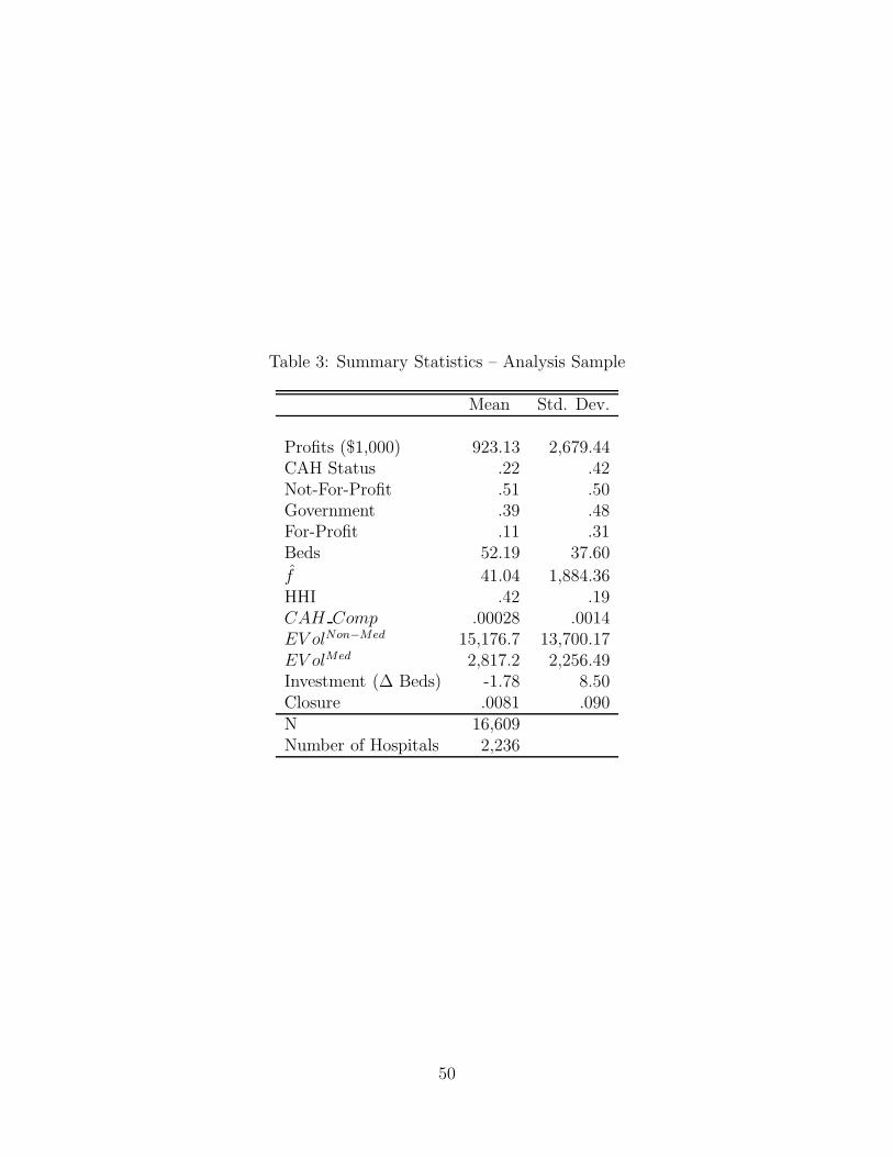
Table 3: Summary Statistics – Analysis Sample

Mean Std. Dev.

Profits ($1,000) 923.13 2,679.44CAH Status .22 .42Not-For-Profit .51 .50Government .39 .48For-Profit .11 .31Beds 52.19 37.60

f 41.04 1,884.36HHI .42 .19CAH Comp .00028 .0014EV olNon−Med 15,176.7 13,700.17EV olMed 2,817.2 2,256.49Investment (∆ Beds) -1.78 8.50Closure .0081 .090N 16,609Number of Hospitals 2,236

50

Table 4: Summary Statistics in 2005 by CAH Status

CAH Non-CAH

Profits ($1,000) 448.67 1,835.1Not-For-Profit .47 .52Government .49 .32For-Profit .036 .16Beds 22.47 70.17

f -483.31 590.83HHI .3587 .4485CAH Comp .00074 .00032EV olNon−Med 2,247 13,700.17EV olMed 990.0 4,284.6Investment (Beds) -2.03 -.36Closure .0066 .0081N 916 984

51

Table 5: Estimates from MNL Model of Hospital Choice

Variable Medicare S.E. Private S.E.

Distance -.022 .0024 -.043 .0026Distance2/100 -1.48 .22 -.12 .22Dist × Urban -.035 .0025 -.031 .0026Dist2 × Urban 2.96 .22 2.69 .22Closest 2.61 .067 2.08 .072Closest × Beds -.0025 .00016 -.0017 .00017Closest × Urban -.49 .061 -.61 .065CAH -14.68 4.12 -40.71 4464CAH × Closest 12.36 3.85 36.37 4464CAH × Dist 2.61 .067 .18 .066Beds .011 .00014 .012 .00013Beds2 -.00076 .0000020 -.00077 .000018Teaching -1.31 .040 -1.31 .039Closest × Dist -.032 .00019 -.032 .0019Teach × Dist .0092 .00089 .0098 .00082Beds × Dist -.000018 1.86 × 10−6 -.000021 1.81 × 10−6

N 29,536 26,365Likelihood -86,427 -72,765

52

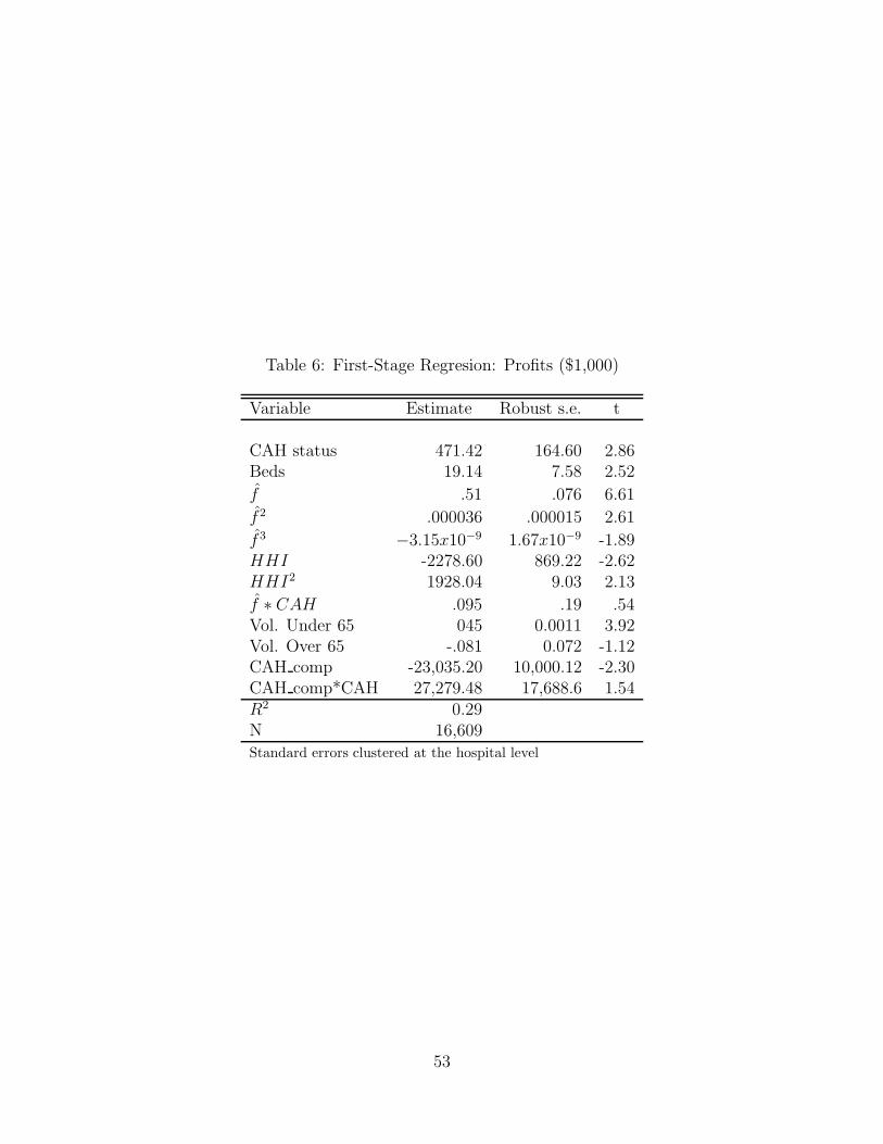
Table 6: First-Stage Regresion: Profits ($1,000)

Variable Estimate Robust s.e. t

CAH status 471.42 164.60 2.86Beds 19.14 7.58 2.52

f .51 .076 6.61

f 2 .000036 .000015 2.61

f 3 −3.15x10−9 1.67x10−9 -1.89HHI -2278.60 869.22 -2.62HHI2 1928.04 9.03 2.13

f ∗ CAH .095 .19 .54Vol. Under 65 045 0.0011 3.92Vol. Over 65 -.081 0.072 -1.12CAH comp -23,035.20 10,000.12 -2.30CAH comp*CAH 27,279.48 17,688.6 1.54R2 0.29N 16,609Standard errors clustered at the hospital level

53

Table 7: First-Stage Regresion: CAH Conversion

Variable Estimate Robust s.e. z

NFP .90 .23 3.84Gov .78 .23 3.32Beds .015 .014 1.12Beds2 -.0022 .0002 -10.78

f -.17 .33 -.53

f 2 -.054 .025 -2.19

f 3 .002 .002 0.98HHI .45 1.61 .28

f ∗ HHI 1.42 1.27 1.11

f ∗ Beds -.0093 .0041 -2.27Vol. Under 65 0.000049 0.000016 3.43Vol. Over 65 -.00028 0.000097 -2.85CAH Comp 27.0 16.94 1.59x -.25 0.0083 -30.48Constant -1.34 .54 -2.47Log Likelihood -1,895.5N 11,155Standard errors clustered at the hospital level

54

Table 8: First-Stage Regression: Investment

Variable Estimate Robust s.e. zNFP .90 .23 3.84Gov .78 .23 3.32CAH status -.072 .015 -4.59CAH status*Beds 1.88 .46 4.07Beds -.0039 .0054 -.71Beds2 -.000026 .000027 -.96

f -.045 .18 -.25

f 2 .0041 .58 .71

f 3 -.00027 .00047 -0.58HHI -.46 1.27 -.37

f ∗ HHI .16 .73 .22

f ∗ Beds .00047 .00097 .48Vol. Under 65 0.000016 0.000013 1.27Vol. Over 65 -.000023 0.000084 -.28CAH Comp 8.63 46.86 .18Constant -1.34 .54 -2.47x 6.06 .15 85.08σx 19.10 .22 40.48Log Likelihood -16,327.6N 14,028

55

Table 9: Parameter Estimates Dynamic Oligopoly Equilibrium

Variable Estimate Bootstrapped s.e.

αNFPv -76 (26)

αNFPp 2984 (1616)

αGovv -70 (22)

αGovp 2622 (1274)

1x > 0 −200 (100)1x > 0x 3414 (1105)1x > 0x2 .480 (.311)1x < 0 1.803 (.872)1x < 0x -2363 (717)1x < 0x2 20.5 (15.3)1x < 0xε 1558 (561)σ 1090 (377)γ−1 99 (90)

56