Embed Size (px)
Citation preview
KYB ERNET IK A — VO LUME 4 9 ( 2 0 1 3 ) , NUMBER 1 , PAGES 4 0 – 5 9
GOODNESS-OF-FIT TEST FOR THE ACCELERATEDFAILURE TIME MODEL BASED ON MARTINGALERESIDUALS
Petr Novak
The Accelerated Failure Time model presents a way to easily describe survival regressiondata. It is assumed that each observed unit ages internally faster or slower, depending onthe covariate values. To use the model properly, we want to check if observed data fit themodel assumptions. In present work we introduce a goodness-of-fit testing procedure based onmodern martingale theory. On simulated data we study empirical properties of the test forvarious situations.
Keywords: accelerated failure time model, survival analysis, goodness-of-fit
Classification: 62N01, 62N03
1. INTRODUCTION
Let us observe survival data representing time which passes from beginning of an ex-periment until some pre-defined failure. We suppose that the data may be incompletein a way that some objects may be removed from the observation prior to reaching thefailure, which we call right censoring. We want to model the dependence of the timeto failure on available covariates. The Accelerated Failure Time model (AFT, see [2])presents an alternative to the most widely used and well described Cox proportionalhazard model (see [3]). In the AFT model, we assume the log-linear dependence
log T ∗i = −ZTi β0 + εi,
where T ∗i , i = 1, . . . , n, are the real failure times, Zi = (Zi1, . . . , Zip)T covariates, β0 thevector of real parameters and εi are iid random variables with an unknown distribution.Denote Ci the censoring times, Ti = min(T ∗i , Ci) the times of the end of observationand ∆i = I(T ∗i ≤ Ci) noncensoring indicators. Suppose that T ∗i and Ci are independentfor all i given Zi, and that the censoring distribution does not depend on the regressionparameters. We observe independent data (Ti,∆i, Zi), i = 1, . . . , n.
We assume T ∗i to have a continuous distribution. Denote Fi(t) = P (T ∗i ≤ t) theirdistribution function, fi(t) density, Si(t) = 1 − Fi(t) the survival function, αi(t) =limh↘0 P (t ≤ T ∗i < t + h|T ∗i ≥ t)/h = fi(t)/Si(t) the hazard function and Ai(t) =
Goodness-of-fit test for the AFT model based on martingale residuals 41
∫ t
0αi(s) ds the cumulative hazard. For the AFT model, we have
αi(t) = α0(exp(ZTi β0)t) exp(ZT
i β0).
The baseline hazard α0(t) is the hazard rate of exp(εi), is completely unknown and willbe estimated nonparametrically.
The data may be represented as counting processes, denote Ni(t) = I(Ti ≤ t, ∆i = 1),Yi(t) = I(t ≤ Ti), intensities λi(t) = Yi(t)αi(t) and cumulative intensities Λi(t) =∫ t
0λi(s) ds. All functions and processes are studied on an interval t ∈ [0, τ ], where τ < ∞
is some point beyond the last observed survival time. It can be shown, that under themodel assumptions, Λi(t) are the compensators of corresponding processes Ni(t) withrespect to Ft = σ {Ni(s), Yi(s),Zi, 0 ≤ s ≤ t, i = 1, . . . , n} (see [5]). Therefore Mi(t) :=Ni(t) − Λi(t) are Ft-martingales (Doob-Meyer decomposition). The log-likelihood forthe data can be then rewritten with the help of the counting processes as
l(t) =n∑
i=1
∫ t
0
(log(αi(s)) dNi(s)− Yi(s)αi(s) ds) ,
and by taking the derivative with respect to model parameters we get the score processU(t, β). For estimation of the parameters we solve the equations U(β) ≡ U(τ,β) = 0.
To obtain reliable estimates, the model assumptions must be met. However, the datacan deviate from the model, for example if the dependence is different than log-linear orif we neglected one or more covariates. To check if the model holds, one must considersome goodness-of-fit testing procedure. In section 2, we present a goodness-of-fit statisticfor the AFT model based on martingale approach and resampling techniques.
The model can also be generalized to accommodate time-varying covariates. In sec-tion 3 we explore the approach proposed by Cox and Oakes [4] and further studied byLin and Ying [9] and we present a generalization of the goodness-of-fit test statistic. Onsimulated examples we study the empirical properties of the test in various situationsfor both time-invariant and time-dependent covariates in section 4.
2. THE TEST STATISTIC – TIME-INVARIANT COVARIATES
In the case of fixed covariates, it is possible to employ methods based on classic linear re-gression. One can compute the residuals ri = log Ti +ZT
i β (for uncensored observations,some adjustment is needed for censored data, see Buckley and James [2]), divide intosubsets i. e. by the values of one of the covariates and check the equality of the meansof these subsets with t-test or Wilcoxon test. This method is very straightforward andone can easily get an idea whether the dependence on each covariate is well describedby the AFT model. The downside is that the residuals are neither independent noridentically distributed, and therefore the mentioned two-sample tests do not yield exactresults. Also it cannot be adapted outright to accommodate time-varying covariates butone must take into account the type of dependence.
42 P. NOVAK
Bagdonavicius and Nikulin [1], p. 234, present a method for testing the model withrepeated observations under each (possibly stepwise) covariate setting. This is useful inindustrial testing, where the covariates often represent stress levels and can be set asdesired.
Goodness-of-fit procedures based on sums of martingale residuals were proposed byLin and Spiekerman [6] and Bagdonavicius and Nikulin [1], p. 252 for the AFT modelwith parametric baseline hazard and by Lin et al (1993) [7] for the Cox proportionalhazards model. Here we propose a similar testing procedure also for the AFT model.
We use similar notation as Lin et al (1998) [8], using time-transformed countingprocesses. Let
N∗i (t, β) = Ni(te−ZT
i β), Y ∗i (t, β) = Yi(te−ZT
i β), i = 1, . . . , n.
S∗0 (t, β) =n∑
i=1
Y ∗i (t, β), S∗1 (t, β) =
n∑i=1
Y ∗i (t, β)Zi,
E∗(t, β) =S∗1 (t, β)S∗0 (t, β)
, A0(t, β) =∫ t
0
J(s)S∗0 (t, β)
dN∗• (s, β),
for J(s) = I(S∗0 (t, β) > 0). A0(t, β) is the well-known Nelson–Aalen estimator of A0(t).With some algebra, the score process may be rewritten as
U(t, β) =n∑
i=1
∫ t
0
Q0(s)(Zi − E∗(s, β)) dN∗i (s, β),
with Q0(s) = ( sα′0(s)α0(s)
+ 1). The estimated parameters β are taken as those minimizing‖U(β)‖, because the score process is not continuous in β. It can be shown, that alsowith other choices of Q(s, β), such as Q1 ≡ 1 or Q2(s, β) = 1
nS∗0 (s, β), the estimatedparameters are consistent and n
12 (β−β0) converge to a zero mean Gaussian process [8].
In further examples, we use simply Q1 ≡ 1. Denote the martingale residuals
M∗i (t, β) = N∗
i (t, β)−∫ t
0
Y ∗i (s, β) dA0(s)
and their empirical counterparts
M∗i (t, β) = N∗
i (t, β)−∫ t
0
Y ∗i (s, β) dA0(s, β).
When the model holds, the martingale residuals should fluctuate around zero, otherwisethey would deviate from zero systematically. The proposed test process is
W (t) = n−12
n∑i=1
wiM∗i (t, β),
where wi := f(Zi)I(Zi ≤ z) are weights with a bounded function f and a vector ofconstants z. There are many possibilities how to choose the weights, most simple choice
Goodness-of-fit test for the AFT model based on martingale residuals 43
is to set f(Zi) = Zi or f(Zi) ≡ 1 and the elements zk of the vector z as quantiles ofcorresponding covariates or no truncation (z = ∞). One can also try using the test withvarious weights and compare the results, see 4.1.
The idea of the test is to measure the distance of the process from zero, which canbe done by computing
supt∈[0,τ ]
|W (t)| or supt∈[δ,τ ]
∣∣∣ W (t)√varW (t)
∣∣∣with a suitable variance estimator and some small positive number δ to avoid possibleproblems at the edges.
As we show later, under the null hypothesis, the asymptotic distribution of W (t) isa zero mean Gaussian process with a covariance function which is difficult to obtain.To assess whether the difference from zero is significant for given data, it is possible todevise a process W (t) which has the same limiting distribution under the null hypothesisand is easy to replicate. Denote
Sw(t, β) =∑
i
wiY∗i (s, β), E∗
w(t, β) =S∗w(t, β)S∗0 (t, β)
fN (t) =1n
∑i
∆iwif0(t)tZi, fY (t) =1n
∑i
wig0(t)tZi, (1)
where f0(t) and g0(t) are the baseline densities of eεi and TieZT
i β0 , respectively. LetfN and fY be their empirical counterparts with kernel estimates f0(t) and g0(t). Thequantities exp(εi) can be consistently estimated by exp(ri), with ri being the modifiedregression residuals of [2]. Or we can estimate their distribution by resampling fromF0(t) = 1 − e−A0(t,β). Estimates for Tie
ZTi β0 can be obtained by inserting the esti-
mated parameters β. As for the kernel estimate, it suffices to take Gaussian kernel withSilverman’s commonly used bandwith 1.06σn−1/5 (Silverman, 1986 [12]).
With some algebra, it can be shown that
U(t, β0) =n∑
i=1
∫ t
0
Q(s, β0)(Zi − E∗(s, β0)) dM∗i (s, β0).
Take Gi, i = 1, . . . , n as iid standard normals, let
UGw (t, β) =
n∑i=1
∫ t
0
Q(s, β)(wi − E∗w(s, β)) dM∗
i (s, β)Gi,
UG(t, β) =n∑
i=1
∫ t
0
Q(s, β)(Zi − E∗(s, β)) dM∗i (s, β)Gi.
44 P. NOVAK
Take β∗ as the solution of the equation
U(β) = UG(β).
It is of note, that n12 (β − β∗) has the same limiting distribution as n
12 (β − β0) (see [8]),
which is useful for approximating the distribution of β. Now we have all the componentsneeded to introduce the main result:
Theorem 2.1. Under the assumptions (i) – (vi) from the Appendix, given the observeddata (Ni(t), Yi(t), Zi), i = 1, . . . , n, the process W (t) from above has asymptotically thesame distribution as
W (t) =1√n
UGw (t, β)−
√n
(fN (t) +
∫ t
0
fY (s) dA0(s, β))T
(β − β∗)
− 1√n
∫ t
0
Sw(s, β) d(A0(s, β)− A0(s, β∗)).
P r o o f . The proof is deferred into the Appendix. �
We can now compute W (t) for the studied data set and replicate W (t) many times.The desired p-value p of the test is the proportion of cases, in which the statisticscomputed from the replicated W (t) exceed the statistic computed from W (t). If p < α,we reject the hypothesis that the data follow the AFT model. The variance for thestandardised variant can be computed directly from the resampled processes.
It is also possible to divide the interval [0, τ ] into k subintervals, i. e. quartiles, andcompute the statistic in each of the parts separately and obtain k p-values p1, . . . , pk.One possibility is then to reject the hypothesis whenever we would reject in one of thesubintervals (if min(p1, . . . , pk) < α), which can lead to violating the general level ofsignificance of the test. Another possibility is to use a Bonferroni approximation formultiple-testing and reject only if min(p1, . . . , pk) < α/k.
3. THE TEST STATISTIC – TIME-VARYING COVARIATES
We can also work with time-dependent covariates Zi(t). Cox and Oakes [4] and Lin andYing [9] proposed representing the failure times via following time transformation:
eεi = hi(T ∗i , β0) =∫ T∗
i
0
eZTi (s)β0 ds,
where εi are (iid) and Zi(s) = (Zi1(s), . . . , Zip(s))T is a p-dimensional covariate process.Take the transformed counting processes as
N∗+i (t, β) = ∆iI(hi(Ti, β) ≤ t), Y ∗+
i (t, β) = I(hi(Ti, β) ≥ t).
We can then define the processes S∗+0 , S∗+1 , E∗+, A+0 , M∗+
i (t, β) and U+(t, β) in thesame way as their equivalents in the case with the fixed covariates, using N∗+
i and Y ∗+i
Goodness-of-fit test for the AFT model based on martingale residuals 45
instead of N∗i and Y ∗
i . Constructing the test is not entirely similar, because the weightswi = f(Zi(t))I(Zi(t) ≤ z) would be time-dependent. For practical reasons, we workhere with time-invariant weights, but it could be also shown that it is possible to usetime-varying weights if they are predictable.
With appropriate weights and transformed counting processes we compute S∗+w , E∗+w ,
UG+w and UG+ in the same way as above. Because eZT
i (s)β is positive, hi(t, β) is increas-ing in t. Therefore for each fixed β an inverse function h−1
i (t, β) can be found, for whichh−1
i (hi(t, β), β) = hi(h−1i (t, β), β) = t. Let again f0 and g0 be the density functions of
hi(T ∗i , β0) and hi(Ti, β0), respectively. Denote
f+N (t) =
1n
∑i
∆iwif0(t)∂
∂β
(− hi(h−1
i (t, β), β0))
β=β0
, (2)
f+Y (t) =
1n
∑i
wig0(t)∂
∂β
(− hi(h−1
i (t, β), β0))
β=β0
(3)
and their empirical counterparts f+N (t) and f+
Y (t) obtained by inserting β and kernelestimates f0 and g0. Again, hi(Ti, β0) can be simply estimated by inserting β. The esti-mation of eεi = hi(T ∗i , β0) can be done similarly as in the case with constant covariatesbut is not as straightforward as one has to take into account the type of dependence, orone can estimate the distribution by using F+
0 (t) = 1− e−A+0 (t,β)
Theorem 3.1. Suppose that (i) – (vi) rewritten for the modified variables and processesand also the assumptions (C1) – (C3) for Zi(t) (Lin and Ying [9], see Appendix) hold.Suppose that for fixed β the image of hi(t, β), t ∈ [0,∞] does not depend on β. Letwi = f(Zi(t0))I(Zi(t0) ≤ z) for a fixed time-point t0.Then given the data (Ni(t), Yi(t), Zi(t)), i = 1, . . . , n, the resampled process W+(t)constructed in the same way as W (t) with modified components from above has asymp-totically the same distribution as W+(t) = 1√
n
∑wiM
∗+i (t).
P r o o f . The proof is deferred into the Appendix. �
Now it is possible to perform the test in the same way as in the case with constantcovariates by computing the observed process W (t) and comparing with the replicatedprocesses W (t).
The simplest case would be, if the covariate represents an additional influence whichis added in given time si for each observed individual,
Zi(t) ={
1 t > si
0 t ≤ si.
This means that at the time si the observed individual starts to age faster or slower.The covariate processes have clearly bounded variation. We get
hi(t, β) = min(t, si) + eβ(t− si)+, h−1i (t, β) = min(t, si) + e−β(t− si)+.
46 P. NOVAK
The weights for W+(t) can be chosen as wi = I(si ≤ z) for some z, i. e. z = median(si)etc. Or we can simply sum all the residuals (wi ≡ 1).
In this case, we have
∂
∂β
(− hi(h−1
i (t, β), β0))
β=β0
= − ∂
∂β
(min(t, si) + eβ0−β(t− si)+
)β=β0
= (t− si)+,
therefore f+N (t) and f+
Y (t) are easy to compute.
Also the model with constant covariates can be viewed as a special case, with
hi(t, β) = teZTi β , h−1
i (t, β) = te−ZTi β ,
therefore
∂
∂β
(− hi(h−1
i (t, β), β0))
β=β0
= − ∂
∂β
(teZT
i (β0−β))
β=β0
= tZTi ,
and inserting into 2 and 3 we get fN (t) and fY (t) as in 1.
4. SIMULATION STUDY
We shall use the proposed test in various situations. We want to study whether thetest holds its level of significance and the empirical power of the test against certainalternatives for various sample sizes. Each time we consider noncensored data and datawith about one quarter of the observations randomly and independently censored. As thetest statistic, we took sup |W (t)| and sup
∣∣∣ W (t)√cvarW (t)
∣∣ with the variance estimated from the
resampled processes. Both statistics were computed over the whole time interval and overfour separated subintervals divided by the quartiles of Tie
Ziβ or hi(Ti, β) respectively.The p-value is taken as the proportion of samples in which the replicated statistics exceedthe observed one. For the supremum over the whole interval, we reject the hypothesisif the p-value is lower than the significance level of α = 5%. If we compute the p-valuesover the quartiles separately, we reject firstly when min(p1, p2, p3, p4) < α/4, using theBonferroni correction. Each time, 500 samples were generated and for each sample, W (t)was generated 200×. To examine the empirical power, we generate data from differentmodels and observe the proportion of rightfully rejected samples. To see if the tests holdthe significance level, we generate from the AFT model itself and observe the proportionof wrongfully rejected samples.
4.1. Constant covariates
First, we generated data from the AFT model itself, with lognormal baseline hazardLN(µ = 5, σ2 = 1), β = 1 and one covariate Zi generated as (iid) from N(3, 1).Censoring was generated independently in the same way with baseline LN(6.5,1). Wecompare weights with f(Zi) as either Zi or equal to 1 and z as either the sample medianof Zi or infinity (no observations left out). Each time, 500 samples of 1000 observationswere tested (Table 1).
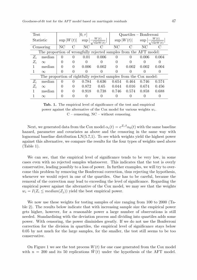
Goodness-of-fit test for the AFT model based on martingale residuals 47
Test [0, τ ] Quartiles – BonferroniStatistic sup |W (t)| sup
∣∣ W (t)√cvarW (t)
∣∣ sup |W (t)| sup∣∣ W (t)√cvarW (t)
∣∣Censoring NC C NC C NC C NC C
The proportion of wrongfully rejected samples from the AFT model:Zi median 0 0 0.01 0.006 0 0 0.006 0.004Zi ∞ 0 0 0 0 0 0 0 01 median 0 0 0.006 0.002 0 0.002 0.002 0.0041 ∞ 0 0 0 0 0 0 0 0
The proportion of rightfully rejected samples from the Cox model:Zi median 0 0 0.784 0.636 0.654 0.464 0.746 0.574Zi ∞ 0 0 0.872 0.65 0.044 0.016 0.674 0.4561 median 0 0 0.918 0.738 0.746 0.574 0.858 0.6881 ∞ 0 0 0 0 0 0 0 0
Tab. 1. The empirical level of significance of the test and empirical
power against the alternative of the Cox model for various weights wi.
C – censoring, NC – without censoring.
Next, we generated data from the Cox model αi(t) = eZiβα0(t) with the same baselinehazard, parameter and covariates as above and the censoring in the same way withlognormal baseline distribution LN(5.7,1). To see which weights yield the highest poweragainst this alternative, we compare the results for the four types of weights used above(Table 1).
We can see, that the empirical level of significance tends to be very low, in somecases even with no rejected samples whatsoever. This indicates that the test is overlyconservative, leading possibly to a loss of power. In further examples, we will try to over-come this problem by removing the Bonferroni correction, thus rejecting the hypothesis,whenever we would reject in one of the quartiles. One has to be careful, because theremoval of the correction may lead to exceeding the level of significance. Regarding theempirical power against the alternative of the Cox model, we may see that the weightswi = I(Zi ≤ median(Zj)) yield the best empirical power.
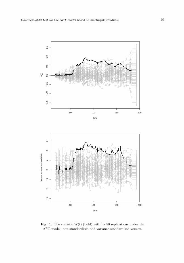
We now use these weights for testing samples of size ranging from 100 to 2000 (Ta-ble 2). The results below indicate that with increasing sample size the empirical powergets higher, however, for a reasonable power a large number of observations is stillneeded. Standardising with the deviation process and dividing into quartiles adds somepower. With censoring, the power diminishes greatly. If we do not use the Bonferronicorrection for the division in quartiles, the empirical level of significance stays below0.05 by not much for the large samples, for the smaller, the test still seems to be tooconservative.
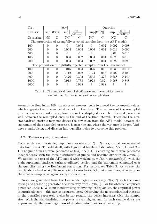
On Figure 1 we see the test process W (t) for one case generated from the Cox modelwith n = 200 and its 50 replications W (t) under the hypothesis of the AFT model.
48 P. NOVAK
Test [0, τ ] QuartilesStatistic sup |W (t)| sup
∣∣ W (t)√cvarW (t)
∣∣ sup |W (t)| sup∣∣ W (t)√cvarW (t)
∣∣Censoring NC C NC C NC C NC C
The proportion of wrongfully rejected samples from the AFT model:100 0 0 0 0.004 0 0.002 0.002 0.008200 0 0 0.004 0.004 0.006 0.002 0.014 0.006500 0 0 0 0 0 0.01 0.0141000 0 0 0.006 0.002 0.004 0.004 0.026 0.0182000 0 0 0.004 0.004 0.002 0.004 0.022 0.026
The proportion of rightfully rejected samples from the Cox model:100 0 0 0.016 0.004 0.026 0.018 0.036 0.014200 0 0 0.112 0.042 0.124 0.056 0.202 0.100500 0 0 0.476 0.302 0.558 0.376 0.688 0.4441000 0 0 0.918 0.738 0.928 0.82 0.968 0.8482000 0 0 1 0.998 1 0.988 1 1
Tab. 2. The empirical level of significance and the empirical power
against the Cox model for various sample sizes.
Around the time index 100, the observed process tends to exceed the resampled values,which suggests that the model does not fit the data. The variance of the resampledprocesses increases with time, however in the displayed case the observed process iswell between the resampled ones at the end of the time interval. Therefore the non-standardised statistic may not detect the deviation from the AFT model because thesupremum of the resampled processes is near the end where the variance is larger. Vari-ance standardising and division into quartiles helps to overcome this problem.
4.2. Time-varying covariates
Consider data with a single jump in one covariate, Zi(t) = I(t > si). First, we generateddata from the AFT model itself, with lognormal baseline distribution LN(5, 1) and β =1. The jump times si were generated as (iid) LN(4, 1). Censoring times were generatedindependently with the same distribution of jumps and baseline distribution LN(6, 1).We applied the test of the AFT model with weights wi = I(si ≤ median(sj)), with theplain supremum statistic, variance-adjusted version and the supremum computed overthe quartiles using the Bonferroni correction. For results, see Table 3. As we see, thetest holds its level of significance is in all cases below 5%, but sometimes, especially forthe smaller samples, is again overly conservative.
Next, we generated from the Cox model αi(t) = exp(Zi(s)β)α0(t) with the samesetting and censoring generated the same way from LN(6, 1). For the obtained empiricalpower see Table 4. Without standardising or dividing into quartiles, the empirical poweris surprisigly zero – this fact is discussed later. Observing the nonstandardised statisticin the quartiles separately yields better results, the power increases with the samplesize. With the standardising, the power is even higher, and for each sample size staysapproximately the same regardless of dividing into quartiles or censoring.
Goodness-of-fit test for the AFT model based on martingale residuals 49
50 100 150 200
−1.
5−
1.0
−0.
50.
00.
51.
01.
5
time
W(t
)
50 100 150 200
−6
−4
−2
02
46
time
Var
ianc
e−st
anda
rdis
ed W
(t)
Fig. 1. The statistic W(t) (bold) with its 50 replications under the
AFT model, non-standardised and variance-standardised version.
50 P. NOVAK
Test [0, τ ] Quartiles – BonferroniStatistic sup |W (t)| sup
∣∣ W (t)√cvarW (t)
∣∣ sup |W (t)| sup∣∣ W (t)√cvarW (t)
∣∣Censoring NC C NC C NC C NC C100 0 0 0.01 0.004 0.004 0 0.004 0.004200 0 0 0.014 0.02 0.006 0.01 0.004 0.01500 0 0 0.022 0.02 0.002 0.004 0.014 0.0161000 0 0 0.028 0.008 0 0.004 0.016 0.0042000 0 0 0.048 0.028 0.012 0.012 0.036 0.028
Tab. 3. The empirical level of significance when generating from the
AFT model with a time-varying covariate.
Test [0, τ ] Quartiles – BonferroniStatistic sup |W (t)| sup
∣∣ W (t)√cvarW (t)
∣∣ sup |W (t)| sup∣∣ W (t)√cvarW (t)
∣∣Censoring NC C NC C NC C NC C100 0 0 0.238 0.218 0.132 0.128 0.178 0.16200 0 0 0.754 0.704 0.38 0.298 0.662 0.584500 0 0 1 0.998 0.846 0.808 0.996 0.9961000 0 0 1 1 1 0.998 1 12000 0 0 1 1 1 1 1 1
Tab. 4. The empirical power against the Cox model with a
time-varying covariate.
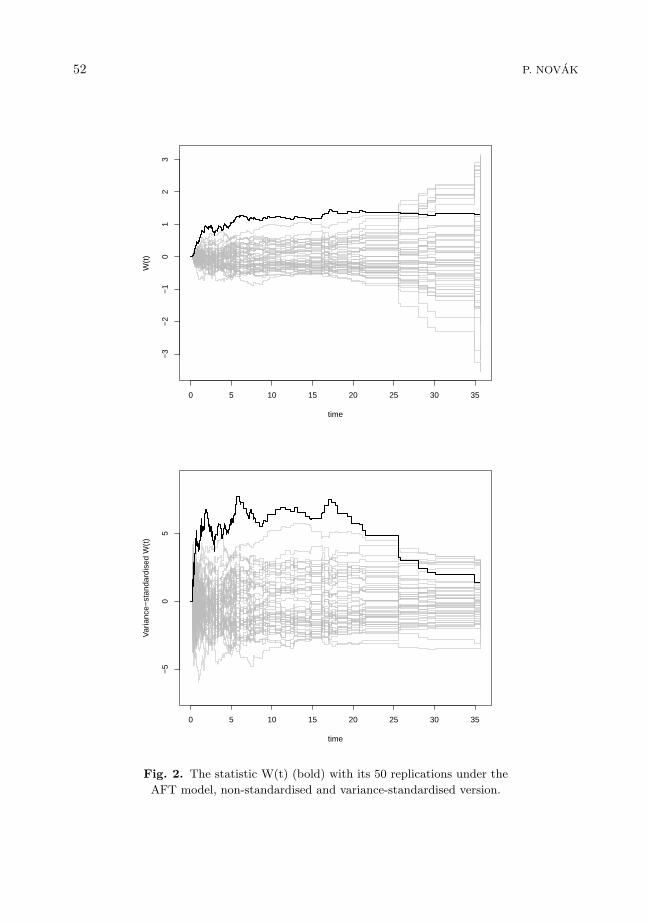
Finally, we generated data from the AFT model with one confounding covariate,with T ∗i satisfying eεi =
∫ T∗i
0eZi(s)β1+Xiβ2 ds with Zi(s) = I(s > si) same as above, Xi
independent, generated from N(3, 1) and β1 = β2 = 1. We test whether the model holdsif we try fitting it using just the covariate Zi(t). For results, see Table 5. For reasonsdiscussed below, using the plain statistic without standardising or dividing into quartiles,the power is very low. However, if we standardise by the standard deviation process orobserve the statistic in the quartiles separately, the empirical power is reasonably high.Also censoring does not reduce the power much.
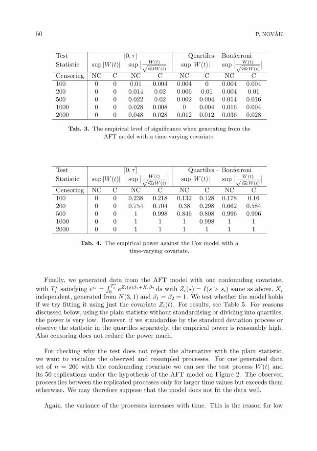
For checking why the test does not reject the alternative with the plain statistic,we want to visualize the observed and resampled processes. For one generated dataset of n = 200 with the confounding covariate we can see the test process W (t) andits 50 replications under the hypothesis of the AFT model on Figure 2. The observedprocess lies between the replicated processes only for larger time values but exceeds themotherwise. We may therefore suppose that the model does not fit the data well.
Again, the variance of the processes increases with time. This is the reason for low
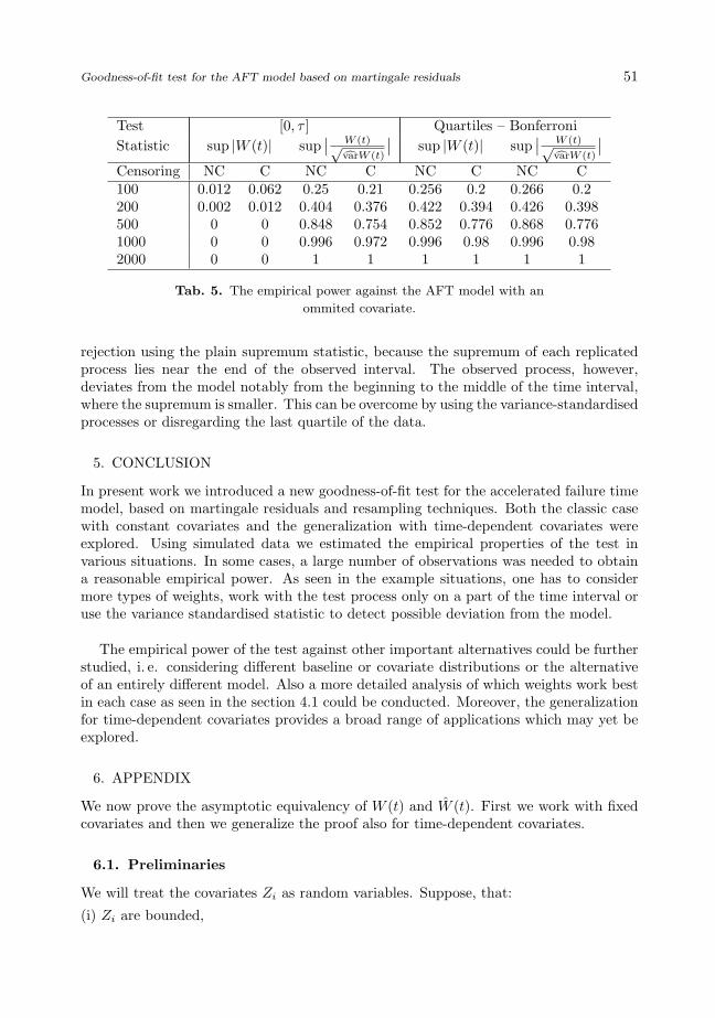
Goodness-of-fit test for the AFT model based on martingale residuals 51
Test [0, τ ] Quartiles – BonferroniStatistic sup |W (t)| sup
∣∣ W (t)√cvarW (t)
∣∣ sup |W (t)| sup∣∣ W (t)√cvarW (t)
∣∣Censoring NC C NC C NC C NC C100 0.012 0.062 0.25 0.21 0.256 0.2 0.266 0.2200 0.002 0.012 0.404 0.376 0.422 0.394 0.426 0.398500 0 0 0.848 0.754 0.852 0.776 0.868 0.7761000 0 0 0.996 0.972 0.996 0.98 0.996 0.982000 0 0 1 1 1 1 1 1
Tab. 5. The empirical power against the AFT model with an
ommited covariate.
rejection using the plain supremum statistic, because the supremum of each replicatedprocess lies near the end of the observed interval. The observed process, however,deviates from the model notably from the beginning to the middle of the time interval,where the supremum is smaller. This can be overcome by using the variance-standardisedprocesses or disregarding the last quartile of the data.
5. CONCLUSION
In present work we introduced a new goodness-of-fit test for the accelerated failure timemodel, based on martingale residuals and resampling techniques. Both the classic casewith constant covariates and the generalization with time-dependent covariates wereexplored. Using simulated data we estimated the empirical properties of the test invarious situations. In some cases, a large number of observations was needed to obtaina reasonable empirical power. As seen in the example situations, one has to considermore types of weights, work with the test process only on a part of the time interval oruse the variance standardised statistic to detect possible deviation from the model.
The empirical power of the test against other important alternatives could be furtherstudied, i. e. considering different baseline or covariate distributions or the alternativeof an entirely different model. Also a more detailed analysis of which weights work bestin each case as seen in the section 4.1 could be conducted. Moreover, the generalizationfor time-dependent covariates provides a broad range of applications which may yet beexplored.
6. APPENDIX
We now prove the asymptotic equivalency of W (t) and W (t). First we work with fixedcovariates and then we generalize the proof also for time-dependent covariates.
6.1. Preliminaries
We will treat the covariates Zi as random variables. Suppose, that:
(i) Zi are bounded,
52 P. NOVAK
0 5 10 15 20 25 30 35
−3
−2
−1
01
23
time
W(t
)
0 5 10 15 20 25 30 35
−5
05
time
Var
ianc
e−st
anda
rdis
ed W
(t)
Fig. 2. The statistic W(t) (bold) with its 50 replications under the
AFT model, non-standardised and variance-standardised version.
Goodness-of-fit test for the AFT model based on martingale residuals 53
(ii) (N∗i , Ci, Zi) are (iid),
(iii) Q, E∗, E∗w and 1
nSw have bounded variation and converge almost surely to contin-uous functions q, e, ew and sw, respectively,
(iv) C∗i = Cie
ZTi β0 have a uniformly bounded density and A0(t) has a bounded second
derivative,
(v) fN (t) = 1n
∑i ∆iwif0(t)tZi and fY (t) = 1
n
∑i wig0(t)tZi have bounded variation
and converge almost surely to f0N (t) and f0
Y (t), respectively,
(vi) The kernel estimates f0 and g0 have a bounded variation and converge in probability,uniformly in t ∈ [0, τ ], to f0 and g0, respectively.
Lin et al [8] shows, that under i-iv for dn → 0:
sup‖β−β0‖<dn
‖U(β)− U(β0) + nA(β − β0)‖/(n12 + n‖β − β0‖) = oP (1), (4)
supt∈[0,τ ],‖β−β0‖<dn
∣∣n 12 (A0(t, β)− A0(t, β0))− bT (t)n
12 (β − β0)
∣∣ = oP (1), (5)
where A =∫ τ
0q(t)E[Y ∗
1 (t, β0)(Z1 − e(t))⊗2] d(α0(t)t) and b(t) = −∫ t
0e(s) d(α0(s)s).
6.2. Convergence for sums of N∗i and Y ∗
i
First, we need to show the asymptotic properties of fN and fY :
Lemma 6.1. Conditional on Zi, under (i) – (vi) for dn → 0:
supt∈[0,τ ],‖β−β0‖<dn
∣∣n− 12
∑wi(N∗
i (t, β)−N∗i (t, β0)) + fT
N (t)n12 (β − β0)
∣∣ = oP (1), (6)
supt∈[0,τ ],‖β−β0‖<dn
∣∣n− 12
∑wi(Y ∗
i (t, β)− Y ∗i (t, β0))− fT
Y (t)n12 (β − β0)
∣∣ = oP (1), (7)
with fN and fY defined in 1.
P r o o f . In this proof we treat Zi as fixed values. We have
n−12
∑wi(N∗
i (t, β)−N∗i (t, β0))
= n−12
∑wi∆i[I(T ∗i eZT
i β ≤ t)− I(T ∗i eZTi β0 ≤ t)]
= n−12
∑wi∆i[I(T ∗i ≤ te−ZT
i β)− I(T ∗i ≤ te−ZTi β0)]
= n−12
∑wi∆i[I(te−ZT
i β0 < T ∗i ≤ te−ZTi β)− I(te−ZT
i β < T ∗i ≤ te−ZTi β0)].
From Lemma 1 of Lin and Ying [9] it follows that uniformly in t ∈ [0, τ ]:
sup‖β−β0‖<dn
˛n−
12
Xwi(N
∗i (t, β)−N∗
i (t, β0))− n−12 E
Xwi(N
∗i (t, β)−N∗
i (t, β0))˛= oP (1)
54 P. NOVAK
and analogically for Y ∗. Hence, it suffices to compute the expectation of the sum ofindicators. For summand i we have E[wi∆i[I(·)− I(·)]] = E[wi∆iE[I(·)− I(·)|∆i]]. Theinner expectation equals to
E[I(te−ZTi β0 < T ∗i ≤ te−ZT
i β)− I(te−ZTi β < T ∗i ≤ te−ZT
i β0)]
= P (t < T ∗i eZTi β0 ≤ teZT
i (β0−β))− P (teZTi (β0−β) < T ∗i eZT
i β0 ≤ t).
Either the first or the second probability is zero, because the cases are mutually exclusive.Assume first, that teZT
i (β0−β) > t, which is equivalent with ZTi β0 > ZT
i β. BecauseT ∗i eZT
i β0 are (iid) with the distribution function F0, we have
P (t < T ∗i eZTi β0 ≤ teZT
i (β0−β)) = F0(teZTi (β0−β))− F0(t)
= f0(t)t(eZTi (β0−β) − 1) + oP (1) = f0(t)tZT
i (β0 − β) + oP (1).
We used the Taylor expansion for β → β0 twice. For ZTi β0 < ZT
i β we get the sameresult, because
−P (teZTi (β0−β) < T ∗i eZT
i β0 ≤ t) = −(F0(t)− F0(teZTi (β0−β))).
Therefore we get the desired result with an conditional expectation with ∆i, we have
n−12
∑wi(N∗
i (t, β)−N∗i (t, β0)) = E[(
1n
∑wi∆if0(t)tZi)T (β0 − β)n
12 ] + oP (1).
Because the censoring is independent, due to SLNN we can replace the expectation withthe observed quantity:
= (1n
∑wi∆if0(t)tZi)T (β0 − β)n
12 + oP (1) = −n
12 fT
N (t)(β − β0) + oP (1).
For the sums of Y ∗i , we have
n−12
∑wi(Y ∗
i (t, β)− Y ∗i (t, β0)) = n−
12
∑wi[I(Ti ≥ te−ZT
i β)− I(Ti ≥ te−ZTi β0)]
= n−12
∑wi[I(t > min(T ∗i eZT
i β0 , CieZT
i β0) ≥ teZTi (β0−β))
− I(teZTi (β0−β) > min(T ∗i eZT
i β0 , CieZT
i β0) ≥ t)].
We assumed that C∗i = Cie
ZTi β0 have a bounded density and therefore Tie
ZTi β0 =
min(T ∗i , Ci)eZTi β0 can be assumed to have a density g0. Computing again the expectation
and using the Taylor expansion, we get
n−12
∑wi(Y ∗
i (t, β)− Y ∗i (t, β0)) = (n−1
∑wig0(t)tZi)T (β − β0)n
12 + oP (1)
= n12 fT
Y (t)(β − β0) + oP (1).
�
Goodness-of-fit test for the AFT model based on martingale residuals 55
6.3. The convergence of the statistic W (t) and W (t)
P r o o f o f T h e o r e m 2.1 . We show the asymptotic equivalence by proving the con-vergence of finite-dimensional distributions and tightness, with the help of multivariatefunctional central limit theorem given by Pollard (see [10]).
W (t) =n−12
∑i
wiM∗i (t, β)
=n−12
∑i
wiM∗i (t, β0) + n−
12
∑i
wi(M∗i (t, β)−M∗
i (t, β0))
=n−12
∑i
wiM∗i (t, β0) + n−
12
∑i
wi(N∗i (t, β)−N∗
i (t, β0))
− n−12
∑i
wi
∫ t
0
(Y ∗
i (s, β) dA0(s, β)− Y ∗i (s, β0) dA0(s)
).
Applying (6) and adding and subtracting Y ∗i (s, β)dA0(s) and Y ∗
i (s, β0)dA0(s, β) we get
W (t) =n−12
∑i
wiM∗i (t, β0)− n
12 fT
N (t)(β − β0)
− n−12
∑i
wi
∫ t
0
Y ∗i (s, β0) d
(A0(s, β)−A0(s)
)− n−
12
∑i
wi
∫ t
0
(Y ∗i (s, β)− Y ∗
i (s, β0)) dA0(s) + oP (1).
With the help of (4) and (5) we have
n12 (A0(s, β)−A0(s)) = n
12 (A0(s, β0)−A0(s)) + bT (t)n
12 (β − β0) + oP (1)
= n12
∑i
∫ t
0
dM∗i (s, β0)
S∗0 (s, β0)+ bT (t)n−
12 A−1U(β0) + oP (1).
We apply (7) on the last term of W (t) and then (4) for n12 (β − β0) = n−
12 A−1U(β0) +
oP (1):
W (t) = n−12
∑i
wiM∗i (t, β0)− n
12
(fN (t) +
∫ t
0
fY (s) dA0(s))T
(β − β0)
− n−12
∑i
∫ t
0
Sw(s, β0)S∗0 (s, β0)
dM∗i (s, β0)− n−
12
∫ t
0
Sw(s, β0) dbT (s)A−1U(β0) + oP (1)
= n−12
∑ ∫ t
0
(wi − E∗w(s, β0)) dM∗
i (s, β0)
− n−12
(fN (t) +
∫ t
0
fY (s) dA0(s) +∫ t
0
1n
Sw(s, β0) db(s))T
A−1U(β0) + oP (1).
56 P. NOVAK
The limiting process can be found similarly as in [8]. Write
UM (t) = n−12
∑M∗
i (t, β0), UMZ(t) = n−12
∑ZiM
∗i (t, β0),
UMW (t) = n−12
∑wiM
∗i (t, β0).
For fixed t, each of the processes is a sum of iid zero-mean terms and therefore thefinite-dimensional convergence of (UM , UMZ , UMW ) follows from multivariate centrallimit theorem. For each t, M∗
i (t, β0), ZiM∗i (t, β0) and wiM
∗i (t, β0) can be written as
sums and products of monotone functions, and therefore are manageable in sense of[10], p. 38. It then follows from the functional central limit theorem ([10], p. 53) that(UM , UMZ , UMW ) is tight and converges weakly to a zero-mean Gaussian process, say(WM ,WMZ ,WMW ). By the Skorokhod – Dudley – Wichura theorem ([11], p. 47), anequivalent process (UM , UMZ , UMW ) in an alternative probability space can be found,in which the convergence becomes almost sure. Because Q(t, β0), E∗(t, β0), E∗
w(t, β0),1nSw(t, β0), fN (t) and fY (t) have bounded variation and converge almost surely to q, e,ew, sw, f0
N (t) and f0Y (t), respectively, then W (t) converges in D[0, τ ] to∫ t
0
dWMW (s)−∫ t
0
ew(s, β0) dWM (s)− cT (t)( ∫ τ
0
q(s) dWMZ −∫ τ
0
q(s)e(s, β0) dWM
),
where c(t) = f0N (t) +
∫ t
0f0
Y (s) dA0(s) +∫ t
0sw(s, β0) db(s), which has zero mean and
covariance function
σ(t1, t2) =E“h Z t1
0(w1 − ew(s, β0)) dM∗
1 (s, β0)− cT (t1)A−1
Z τ
0q(s)[Z1 − e(s, β0)] dM∗
1 (s, β0)i
×h Z t2
0(w1 − ew(s, β0)) dM∗
1 (s, β0)− cT (t2)A−1
Z τ
0q(s)[Z1 − e(s, β0)] dM∗
1 (s, β0)i”
.
For W (t), we have
W (t) =n−12 UG
w (t, β)− n12
„fN (t) +
Z t
0
fY (s) dA0(s, β)
«T
(β − β∗)
− n−12
Z t
0
Sw(s, β) d(A0(s, β)− A0(s, β∗))
=n−12
X Z t
0
(wi − E∗w(s, β)) dM∗
i (s, β)Gi
− n12
„fN (t) +
Z t
0
fY (s) dA0(s, β)
«T
(β − β∗)
− n12
Z t
0
1
nSw(s, β) db(s)(β − β∗) + oP (1)
=n−12
X Z t
0
(wi − E∗w(s, β)) dM∗
i (s, β)Gi
− n−12
„fN (t) +
Z t
0
fY (s) dA0(s, β) +
Z t
0
1
nSw(s, β) db(s)
«T
A−1U(β∗) + oP (1).
We used (4) forn
12 (β − β∗) = n−
12 A−1U(β∗) + oP (1)
Goodness-of-fit test for the AFT model based on martingale residuals 57
and (5) forn
12 (A0(t, β)− A0(t, β∗)) = bT (t)n
12 (β − β∗) + oP (1).
The score process satisfies U(β∗) = UG(β) and therefore we see that W (t) consists of thesame parts as W (t), with β0, M∗
i (t, β0), fN (t) and fY (t) replaced with β, GiM∗i (t, β),
fN (t) and fY (t). The resampled martingale residuals GiM∗i (t, β) have the same distri-
bution as their theoretical counterparts, and the kernel estimates of f0 and g0 convergeuniformly to the real densities. Therefore W (t) has the same limiting finite-dimensionaldistributions as W (t). Tightness follows also by the same arguments as for W (t). �
6.4. Time-varying covariates
We can modify the assumptions (i) – (vi) to accommodate N∗+i , Y ∗+
i and all derivedgeneralized processes. Suppose also, that following assumptions for Zi(t) of Lin andYing [9] hold:
(C1) ∀ i = 1, . . . , n, k = 1, . . . , p: Zik(t) have uniformly bounded total variation, i. e.∃D : Zik(0) +
∫ τ
0|dZik(s)| ≤ D.
Because of (C1), Zik can be decomposed into Zik(t) = Zik(0) + Z+ik(t) − Z−
ik(t), whereZ±
ik(·) are increasing functions with Z±ik(0) = 0.
(C2) There exist η0 > 0 and κ0 > 0, such that ∀ k = 1, . . . , p:
sup|t−s|+‖β1−β2‖≤n−κ0
1n
n∑i=1
|Z±ik(h−1(t, β1))− Z±
ik(h−1(s, β2))| = OP (n−12−η0)
and for dn > 0, dn → 0 exists ε0, such that ∀ k = 1, . . . , p:
sup|t−s|+‖β1−β2‖≤dn
1n
n∑i=1
|Z±ik(h−1(t, β1))− Z±
ik(h−1(s, β2))| = oP (max(dε0n , n−ε0)).
(C3) f0 and f ′0 are bounded,∫ τ
0
(f ′0(s)f0(s)
)2
f(s) ds < ∞ and∫ τ
0xε0f(x) dx < ∞ for some
ε0 > 0.
Then the results (4) and (5) (due to Lin et al [8]) hold for the case of time-dependentcovariates, too. We can also extend (6) and (7):
Lemma 6.2. Suppose that for fixed β the image of hi(t, β), t ∈ [0,∞] does not dependon β. Conditional on Zi, under the assumptions (i) – (vi) rewritten for the the modifiedvariables and processes and (C1) – (C3), for dn → 0:
supt∈[0,τ ],‖β−β0‖<dn
∣∣n− 12
∑wi(N∗+
i (t, β)−N∗+i (t, β0)) + (f+
N (t))T n12 (β − β0)
∣∣ = oP (1),
supt∈[0,τ ],‖β−β0‖<dn
∣∣n− 12
∑wi(Y ∗+
i (t, β)− Y ∗+i (t, β0))− (f+
Y (t))T n12 (β − β0)
∣∣ = oP (1),
58 P. NOVAK
with f+N and f+
Y defined in 2 and 3.
P r o o f o f T h e o r e m 2.1 . We proceed similarly as in the proof of Lemma 6.1:
n−12
∑wi(N∗+
i (t, β)−N∗+i (t, β0))
= n−12
∑wi∆i[I(hi(T ∗i , β) ≤ t)− I(hi(T ∗i , β0) ≤ t)]
= n−12
∑wi∆i[I(T ∗i ≤ h−1
i (t, β))− I(T ∗i ≤ h−1i (t, β0))]
= n−12
∑wi∆i[I(h−1
i (t, β0) < T ∗i ≤ h−1i (t, β))− I(h−1
i (t, β) < T ∗i ≤ h−1i (t, β0))].
Again, it can be shown that it suffices to compute the expectation of the sum of indicators([9], Lemma 1). For each part, the inner conditional expectation is
E[I(h−1i (t, β0) < T ∗i ≤ h−1
i (t, β))− I(h−1i (t, β) < T ∗i ≤ h−1
i (t, β0))]
= P (t < hi(T ∗i , β0) ≤ hi(h−1i (t, β), β0))− P (hi(h−1
i (t, β), β0) < hi(T ∗i , β0) ≤ t).
Both cases are mutually exclusive, suppose first that hi(h−1i (t, β), β0) > t. Because
hi(T ∗i , β0) = eεi are (iid), we have
P (t < hi(T ∗i , β0) ≤ hi(h−1i (t, β), β0)) = F0(hi(h−1
i (t, β), β0))− F0(t)
= f0(t)( ∂
∂β
(hi(h−1
i (t, β), β0))
β=β0
)T
(β − β0) + oP (1)
using Taylor expansion for β → β0. For hi(h−1i (t, β), β0) < t we get again the same
result. Inserting into the sum and replacing the expectation with respect to ∆i with theobserved quantity we get
n−12
∑wi(N∗+
i (t, β)−N∗+i (t, β0))
=( 1
n
∑wi∆if0(t)
∂
∂β
(hi(h−1
i (t, β), β0))
β=β0
)T
(β − β0)n12 + oP (1)
= −n12 (f+
N (t))T (β − β0) + oP (1).
In similar way we obtain also the result for sums of Y ∗+i . �
P r o o f o f T h e o r e m 3.1 . The proof is analogous to the proof of Theorem 2.1, usingLemma 6.2. �
ACKNOWLEDGEMENT
This work was supported by grants of the Ministry of Education, Youth and Sports of theCzech Republic 1M06047 and SVV 261315/2011.
(Received December 12, 2011)
Goodness-of-fit test for the AFT model based on martingale residuals 59
R E FER E NCE S
[1] V. Bagdonavicius and M. Nikulin: Accelerated Life Models. Chapman and Hall / CRC,Boca Raton 2002.
[2] J. Buckley, and I. R. James: Linear regression with censored data. Biometrika 66 (1979),429–436.
[3] D. R. Cox: Regression models and life tables. J. Roy. Statist. Soc. Ser. B 34 (1972),187–220.
[4] D. R. Cox and D.Oakes: Analysis of Survival Data. Chapman and Hall / CRC, BocaRaton1984.
[5] T. R. Fleming and D. P. Harrington: Counting Processes and Survival Analysis. Wiley,New York 1991.
[6] D. Y. Lin and C. F. Spiekerman: Model checking techniques for parametric regressionwith censored data. Scand. J. Statist. 23 (1996), 157–177.
[7] D. Y. Lin, L. J. Wei, and Z. Ying: Checking the Cox model with cumulative sums ofmartingale-based residuals. Biometrika 80 (1993), 557–572.
[8] D. Y. Lin, L. J. Wei, and Z. Ying: Accelerated failure time models for counting processes.Biometrika 85 (1998), 605–618.
[9] D. Y. Lin and Z. Ying: Semiparametric inference for the accelerated life model withtime-dependent covariates. J. Statist. Plann. Inference 44 (1995), 47–63.
[10] D. Pollard: Empirical Processes: Theory and Applications. Hayward, California: IMS1990.
[11] G. R. Shorack and J.A. Wellner: Empirical Processes with Applications to Statistics.Wiley, New York 1986.
[12] B. W. Silverman: Density Estimation for Statistics and Data Analysis. Chapman andHall, London 1986.
Petr Novak, Charles University in Prague, Faculty of Mathematics and Physics, Department of
Probability and Mathematical Statistics, Sokolovska 83, 186 75 Praha 8 and Institute of Infor-
mation Theory and Automation – Academy of Sciences of the Czech Republic, Pod Vodarenskou
vezı 4, 182 08 Praha 8. Czech Republic.
e-mail: [email protected]