Embed Size (px)
Citation preview

A Linear-Time Kernel Goodness-of-Fit Test
Wittawat JitkrittumGatsby Unit, UCL
Wenkai XuGatsby Unit, UCL
Zoltán Szabó∗CMAP, École Polytechnique
Kenji FukumizuThe Institute of Statistical Mathematics
Arthur Gretton∗Gatsby Unit, UCL
AbstractWe propose a novel adaptive test of goodness-of-fit, with computational costlinear in the number of samples. We learn the test features that best indicate thedifferences between observed samples and a reference model, by minimizing thefalse negative rate. These features are constructed via Stein’s method, meaning thatit is not necessary to compute the normalising constant of the model. We analysethe asymptotic Bahadur efficiency of the new test, and prove that under a mean-shiftalternative, our test always has greater relative efficiency than a previous linear-timekernel test, regardless of the choice of parameters for that test. In experiments, theperformance of our method exceeds that of the earlier linear-time test, and matchesor exceeds the power of a quadratic-time kernel test. In high dimensions and wheremodel structure may be exploited, our goodness of fit test performs far better thana quadratic-time two-sample test based on the Maximum Mean Discrepancy, withsamples drawn from the model.
1 Introduction
The goal of goodness of fit testing is to determine how well a model density p(x) fits an observedsample D = {xi}ni=1 ⊂ X ⊆ Rd from an unknown distribution q(x). This goal may be achieved viaa hypothesis test, where the null hypothesis H0 : p = q is tested against H1 : p 6= q. The problemof testing goodness of fit has a long history in statistics [11], with a number of tests proposed forparticular parametric models. Such tests can require space partitioning [18, 3], which works poorly inhigh dimensions; or closed-form integrals under the model, which may be difficult to obtain, besidesin certain special cases [2, 5, 30, 26]. An alternative is to conduct a two-sample test using samplesdrawn from both p and q. This approach was taken by [23], using a test based on the (quadratic-time)Maximum Mean Discrepancy [16], however this does not take advantage of the known structure of p(quite apart from the increased computational cost of dealing with samples from p).
More recently, measures of discrepancy with respect to a model have been proposed based on Stein’smethod [21]. A Stein operator for p may be applied to a class of test functions, yielding functions thathave zero expectation under p. Classes of test functions can include the W 2,∞ Sobolev space [14],and reproducing kernel Hilbert spaces (RKHS) [25]. Statistical tests have been proposed by [9, 22]based on classes of Stein transformed RKHS functions, where the test statistic is the norm of thesmoothness-constrained function with largest expectation under q . We will refer to this statistic asthe Kernel Stein Discrepancy (KSD). For consistent tests, it is sufficient to use C0-universal kernels[6, Definition 4.1], as shown by [9, Theorem 2.2], although inverse multiquadric kernels may bepreferred if uniform tightness is required [15].2
∗Zoltán Szabó’s ORCID ID: 0000-0001-6183-7603. Arthur Gretton’s ORCID ID: 0000-0003-3169-7624.2Briefly, [15] show that when an exponentiated quadratic kernel is used, a sequence of sets D may be
constructed that does not correspond to any q, but for which the KSD nonetheless approaches zero. In a statisticaltesting setting, however, we assume identically distributed samples from q, and the issue does not arise.
31st Conference on Neural Information Processing Systems (NIPS 2017), Long Beach, CA, USA.

The minimum variance unbiased estimate of the KSD is a U-statistic, with computational costquadratic in the number n of samples from q. It is desirable to reduce the cost of testing, however,so that larger sample sizes may be addressed. A first approach is to replace the U-statistic with arunning average with linear cost, as proposed by [22] for the KSD, but this results in an increase invariance and corresponding decrease in test power. An alternative approach is to construct explicitfeatures of the distributions, whose empirical expectations may be computed in linear time. In thetwo-sample and independence settings, these features were initially chosen at random by [10, 8, 32].More recently, features have been constructed explicitly to maximize test power in the two-sample[19] and independence testing [20] settings, resulting in tests that are not only more interpretable, butwhich can yield performance matching quadratic-time tests.
We propose to construct explicit linear-time features for testing goodness of fit, chosen so as tomaximize test power. These features further reveal where the model and data differ, in a readily inter-pretable way. Our first theoretical contribution is a derivation of the null and alternative distributionsfor tests based on such features, and a corresponding power optimization criterion. Note that thegoodness-of-fit test requires somewhat different strategies to those employed for two-sample andindependence testing [19, 20], which become computationally prohibitive in high dimensions forthe Stein discrepancy (specifically, the normalization used in prior work to simplify the asymptoticswould incur a cost cubic in the dimension d and the number of features in the optimization). Detailsmay be found in Section 3.
Our second theoretical contribution, given in Section 4, is an analysis of the relative Bahadurefficiency of our test vs the linear time test of [22]: this represents the relative rate at which the p-value decreases under H1 as we observe more samples. We prove that our test has greater asymptoticBahadur efficiency relative to the test of [22], for Gaussian distributions under the mean-shiftalternative. This is shown to hold regardless of the bandwidth of the exponentiated quadratic kernelused for the earlier test. The proof techniques developed are of independent interest, and we anticipatethat they may provide a foundation for the analysis of relative efficiency of linear-time tests in thetwo-sample and independence testing domains. In experiments (Section 5), our new linear-time testis able to detect subtle local differences between the density p(x), and the unknown q(x) as observedthrough samples. We show that our linear-time test constructed based on optimized features hascomparable performance to the quadratic-time test of [9, 22], while uniquely providing an explicitvisual indication of where the model fails to fit the data.
2 Kernel Stein Discrepancy (KSD) Test
We begin by introducing the Kernel Stein Discrepancy (KSD) and associated statistical test, asproposed independently by [9] and [22]. Assume that the data domain is a connected open setX ⊆ Rd.Consider a Stein operator Tp that takes in a multivariate function f(x) = (f1(x), . . . , fd(x))> ∈ Rdand constructs a function (Tpf) (x) : Rd → R. The constructed function has the key property that forall f in an appropriate function class, Ex∼q [(Tpf)(x)] = 0 if and only if q = p. Thus, one can usethis expectation as a statistic for testing goodness of fit.
The function classFd for the function f is chosen to be a unit-norm ball in a reproducing kernel Hilbertspace (RKHS) in [9, 22]. More precisely, let F be an RKHS associated with a positive definite kernelk : X × X → R. Let φ(x) = k(x, ·) denote a feature map of k so that k(x,x′) = 〈φ(x), φ(x′)〉F .Assume that fi ∈ F for all i = 1, . . . , d so that f ∈ F × · · · × F := Fd where Fd is equipped withthe standard inner product 〈f ,g〉Fd :=
∑di=1 〈fi, gi〉F . The kernelized Stein operator Tp studied
in [9] is (Tpf) (x) :=∑di=1
(∂ log p(x)∂xi
fi(x) + ∂fi(x)∂xi
)(a)=⟨f , ξp(x, ·)
⟩Fd , where at (a) we use the
reproducing property of F , i.e., fi(x) = 〈fi, k(x, ·)〉F , and that ∂k(x,·)∂xi∈ F [28, Lemma 4.34],
hence ξp(x, ·) := ∂ log p(x)∂x k(x, ·)+ ∂k(x,·)
∂x is inFd. We note that the Stein operator presented in [22]is defined such that (Tpf) (x) ∈ Rd. This distinction is not crucial and leads to the same goodness-of-fit test. Under appropriate conditions, e.g. that lim‖x‖→∞ p(x)fi(x) = 0 for all i = 1, . . . , d, it canbe shown using integration by parts that Ex∼p(Tpf)(x) = 0 for any f ∈ Fd [9, Lemma 5.1]. Basedon the Stein operator, [9, 22] define the kernelized Stein discrepancy as
Sp(q) := sup‖f‖Fd≤1
Ex∼q⟨f , ξp(x, ·)
⟩Fd
(a)= sup‖f‖Fd≤1
⟨f ,Ex∼qξp(x, ·)
⟩Fd = ‖g(·)‖Fd , (1)
2

where at (a), ξp(x, ·) is Bochner integrable [28, Definition A.5.20] as long as Ex∼q‖ξp(x, ·)‖Fd <∞, and g(y) := Ex∼qξp(x,y) is what we refer to as the Stein witness function. The Stein witnessfunction will play a crucial role in our new test statistic in Section 3. When a C0-universal kernel isused [6, Definition 4.1], and as long as Ex∼q‖∇x log p(x)−∇x log q(x)‖2 <∞, it can be shownthat Sp(q) = 0 if and only if p = q [9, Theorem 2.2].
The KSD Sp(q) can be written as S2p(q) = Ex∼qEx′∼qhp(x,x
′), where hp(x,y) :=
s>p (x)sp(y)k(x,y) + s>p (y)∇xk(x,y) + s>p (x)∇yk(x,y) +∑di=1
∂2k(x,y)∂xi∂yi
, and sp(x) :=
∇x log p(x) is a column vector. An unbiased empirical estimator of S2p(q), denoted by S2 =
2n(n−1)
∑i<j hp(xi,xj) [22, Eq. 14], is a degenerate U-statistic under H0. For the goodness-of-fit
test, the rejection threshold can be computed by a bootstrap procedure. All these properties make S2
a very flexible criterion to detect the discrepancy of p and q: in particular, it can be computed even ifp is known only up to a normalization constant. Further studies on nonparametric Stein operators canbe found in [25, 14].
Linear-Time Kernel Stein (LKS) Test Computation of S2 costs O(n2). To reduce this cost, alinear-time (i.e., O(n)) estimator based on an incomplete U-statistic is proposed in [22, Eq. 17],given by S2
l := 2n
∑n/2i=1 hp(x2i−1,x2i), where we assume n is even for simplicity. Empirically
[22] observed that the linear-time estimator performs much worse (in terms of test power) than thequadratic-time U-statistic estimator, agreeing with our findings presented in Section 5.
3 New Statistic: The Finite Set Stein Discrepancy (FSSD)
Although shown to be powerful, the main drawback of the KSD test is its high computational cost ofO(n2). The LKS test is one order of magnitude faster. Unfortunately, the decrease in the test poweroutweighs the computational gain [22]. We therefore seek a variant of the KSD statistic that can becomputed in linear time, and whose test power is comparable to the KSD test.
Key Idea The fact that Sp(q) = 0 if and only if p = q implies that g(v) = 0 for all v ∈ X if andonly if p = q, where g is the Stein witness function in (1). One can see g as a function witnessingthe differences of p, q, in such a way that |gi(v)| is large when there is a discrepancy in the regionaround v, as indicated by the ith output of g. The test statistic of [22, 9] is essentially given by thedegree of “flatness” of g as measured by the RKHS norm ‖ · ‖Fd . The core of our proposal is to usea different measure of flatness of g which can be computed in linear time.
The idea is to use a real analytic kernel k which makes g1, . . . , gd real analytic. If gi 6= 0 is ananalytic function, then the Lebesgue measure of the set of roots {x | gi(x) = 0} is zero [24]. Thisproperty suggests that one can evaluate gi at a finite set of locations V = {v1, . . . ,vJ}, drawnfrom a distribution with a density (w.r.t. the Lebesgue measure). If gi 6= 0, then almost surelygi(v1), . . . , gi(vJ) will not be zero. This idea was successfully exploited in recently proposedlinear-time tests of [8] and [19, 20]. Our new test statistic based on this idea is called the Finite SetStein Discrepancy (FSSD) and is given in Theorem 1. All proofs are given in the appendix.Theorem 1 (The Finite Set Stein Discrepancy (FSSD)). Let V = {v1, . . . ,vJ} ⊂ Rd be randomvectors drawn i.i.d. from a distribution η which has a density. Let X be a connected open setin Rd. Define FSSD2
p(q) := 1dJ
∑di=1
∑Jj=1 g
2i (vj). Assume that 1) k : X × X → R is C0-
universal [6, Definition 4.1] and real analytic i.e., for all v ∈ X , f(x) := k(x,v) is a real analyticfunction on X . 2) Ex∼qEx′∼qhp(x,x
′) < ∞. 3) Ex∼q‖∇x log p(x) − ∇x log q(x)‖2 < ∞. 4)lim‖x‖→∞ p(x)g(x) = 0.
Then, for any J ≥ 1, η-almost surely FSSD2p(q) = 0 if and only if p = q.
This measure depends on a set of J test locations (or features) {vi}Ji=1 used to evaluate the Steinwitness function, where J is fixed and is typically small. A kernel which is C0-universal and realanalytic is the Gaussian kernel k(x,y) = exp
(−‖x−y‖
22
2σ2k
)(see [20, Proposition 3] for the result
on analyticity). Throughout this work, we will assume all the conditions stated in Theorem 1, andconsider only the Gaussian kernel. Besides the requirement that the kernel be real and analytic,the remaining conditions in Theorem 1 are the same as given in [9, Theorem 2.2]. Note that if the
3
FSSD is to be employed in a setting otherwise than testing, for instance to obtain pseudo-samplesconverging to p, then stronger conditions may be needed [15].
3.1 Goodness-of-Fit Test with the FSSD Statistic
Given a significance level α for the goodness-of-fit test, the test can be constructed so that H0 isrejected when nFSSD2 > Tα, where Tα is the rejection threshold (critical value), and FSSD2 isan empirical estimate of FSSD2
p(q). The threshold which guarantees that the type-I error (i.e., theprobability of rejecting H0 when it is true) is bounded above by α is given by the (1− α)-quantile ofthe null distribution i.e., the distribution of nFSSD2 under H0. In the following, we start by givingthe expression for FSSD2, and summarize its asymptotic distributions in Proposition 2.
Let Ξ(x) ∈ Rd×J such that [Ξ(x)]i,j = ξp,i(x,vj)/√dJ . Define τ (x) := vec(Ξ(x)) ∈ RdJ where
vec(M) concatenates columns of the matrix M into a column vector. We note that τ (x) dependson the test locations V = {vj}Jj=1. Let ∆(x,y) := τ (x)>τ (y) = tr(Ξ(x)>Ξ(y)). Given an i.i.d.sample {xi}ni=1 ∼ q, a consistent, unbiased estimator of FSSD2
p(q) is
FSSD2 =1
dJ
d∑l=1
J∑m=1
1
n(n− 1)
n∑i=1
∑j 6=i
ξp,l(xi,vm)ξp,l(xj ,vm) =2
n(n− 1)
∑i<j
∆(xi,xj), (2)
which is a one-sample second-order U-statistic with ∆ as its U-statistic kernel [27, Section 5.1.1].Being a U-statistic, its asymptotic distribution can easily be derived. We use d→ to denote convergencein distribution.
Proposition 2 (Asymptotic distributions of FSSD2). Let Z1, . . . , ZdJi.i.d.∼ N (0, 1). Let µ :=
Ex∼q[τ (x)], Σr := covx∼r[τ (x)] ∈ RdJ×dJ for r ∈ {p, q}, and {ωi}dJi=1 be the eigenvalues ofΣp = Ex∼p[τ (x)τ>(x)]. Assume that Ex∼qEy∼q∆
2(x,y) < ∞. Then, for any realization ofV = {vj}Jj=1, the following statements hold.
1. Under H0 : p = q, nFSSD2 d→∑dJi=1(Z2
i − 1)ωi.
2. Under H1 : p 6= q, if σ2H1
:= 4µ>Σqµ > 0, then√n(FSSD2 − FSSD2)
d→ N (0, σ2H1
).
Proof. Recognizing that (2) is a degenerate U-statistic, the results follow directly from [27, Section5.5.1, 5.5.2].
Claims 1 and 2 of Proposition 2 imply that under H1, the test power (i.e., the probability of correctlyrejecting H1) goes to 1 asymptotically, if the threshold Tα is defined as above. In practice, simulatingfrom the asymptotic null distribution in Claim 1 can be challenging, since the plug-in estimator ofΣp requires a sample from p, which is not available. A straightforward solution is to draw samplefrom p, either by assuming that p can be sampled easily or by using a Markov chain Monte Carlo(MCMC) method, although this adds an additional computational burden to the test procedure. Amore subtle issue is that when dependent samples from p are used in obtaining the test threshold, thetest may become more conservative than required for i.i.d. data [7]. An alternative approach is to usethe plug-in estimate Σq instead of Σp. The covariance matrix Σq can be directly computed from thedata. This is the approach we take. Theorem 3 guarantees that the replacement of the covariance inthe computation of the asymptotic null distribution still yields a consistent test. We write PH1 for thedistribution of nFSSD2 under H1.
Theorem 3. Let Σq := 1n
∑ni=1 τ (xi)τ
>(xi)− [ 1n∑ni=1 τ (xi)][
1n
∑nj=1 τ (xj)]
> with {xi}ni=1 ∼q. Suppose that the test threshold Tα is set to the (1−α)-quantile of the distribution of
∑dJi=1(Z2
i −1)νi
where {Zi}dJi=1i.i.d.∼ N (0, 1), and ν1, . . . , νdJ are eigenvalues of Σq . Then, underH0, asymptotically
the false positive rate is α. Under H1, for {vj}Jj=1 drawn from a distribution with a density, the test
power PH1(nFSSD2 > Tα)→ 1 as n→∞.
Remark 1. The proof of Theorem 3 relies on two facts. First, under H0, Σq = Σp i.e., the plug-inestimate of Σp. Thus, under H0, the null distribution approximated with Σq is asymptotically
4

correct, following the convergence of Σp to Σp. Second, the rejection threshold obtained from theapproximated null distribution is asymptotically constant. Hence, under H1, claim 2 of Proposition 2implies that nFSSD2 d→∞ as n→∞, and consequently PH1(nFSSD2 > Tα)→ 1.
3.2 Optimizing the Test Parameters
Theorem 1 guarantees that the population quantity FSSD2 = 0 if and only if p = q for any choice of{vi}Ji=1 drawn from a distribution with a density. In practice, we are forced to rely on the empiricalFSSD2, and some test locations will give a higher detection rate (i.e., test power) than others forfinite n. Following the approaches of [17, 20, 19, 29], we choose the test locations V = {vj}Jj=1
and kernel bandwidth σ2k so as to maximize the test power i.e., the probability of rejecting H0 when
it is false. We first give an approximate expression for the test power when n is large.
Proposition 4 (Approximate test power of nFSSD2). Under H1, for large n and fixed r, thetest power PH1
(nFSSD2 > r) ≈ 1 − Φ(
r√nσH1
−√nFSSD2
σH1
), where Φ denotes the cumulative
distribution function of the standard normal distribution, and σH1 is defined in Proposition 2.
Proof. PH1(nFSSD2 > r) = PH1(FSSD2 > r/n) = PH1
(√n FSSD2−FSSD2
σH1>√n r/n−FSSD
2
σH1
).
For sufficiently large n, the alternative distribution is approximately normal as given in Proposition 2.It follows that PH1
(nFSSD2 > r) ≈ 1− Φ(
r√nσH1
−√nFSSD2
σH1
).
Let ζ := {V, σ2k} be the collection of all tuning parameters. Assume that n is sufficiently large.
Following the same argument as in [29], in r√nσH1
− √nFSSD2
σH1, we observe that the first term
r√nσH1
= O(n−1/2) going to 0 as n→∞, while the second term√nFSSD2
σH1= O(n1/2), dominating
the first for large n. Thus, the best parameters that maximize the test power are given by ζ∗ =
arg maxζ PH1(nFSSD2 > Tα) ≈ arg maxζ
FSSD2
σH1. Since FSSD2 and σH1
are unknown, we divide
the sample {xi}ni=1 into two disjoint training and test sets, and use the training set to compute FSSD2
σH1+γ ,
where a small regularization parameter γ > 0 is added for numerical stability. The goodness-of-fittest is performed on the test set to avoid overfitting. The idea of splitting the data into training andtest sets to learn good features for hypothesis testing was successfully used in [29, 20, 19, 17].
To find a local maximum of FSSD2
σH1+γ , we use gradient ascent for its simplicity. The initial points of
{vi}Ji=1 are set to random draws from a normal distribution fitted to the training data, a heuristic wefound to perform well in practice. The objective is non-convex in general, reflecting many possibleways to capture the differences of p and q. The regularization parameter γ is not tuned, and isfixed to a small constant. Assume that∇x log p(x) costs O(d2) to evaluate. Computing ∇ζ
FSSD2
σH1+γ
costs O(d2J2n). The computational complexity of nFSSD2 and σ2H1
is O(d2Jn). Thus, findinga local optimum via gradient ascent is still linear-time, for a fixed maximum number of iterations.Computing Σq costs O(d2J2n), and obtaining all the eigenvalues of Σq costs O(d3J3) (requiredonly once). If the eigenvalues decay to zero sufficiently rapidly, one can approximate the asymptoticnull distribution with only a few eigenvalues. The cost to obtain the largest few eigenvalues alone canbe much smaller.Remark 2. Let µ := 1
n
∑ni=1 τ (xi). It is possible to normalize the FSSD statistic to get a new
statistic λn := nµ>(Σq + γI)−1µ where γ ≥ 0 is a regularization parameter that goes to 0as n → ∞. This was done in the case of the ME (mean embeddings) statistic of [8, 19]. Theasymptotic null distribution of this statistic takes the convenient form of χ2(dJ) (independent ofp and q), eliminating the need to obtain the eigenvalues of Σq. It turns out that the test powercriterion for tuning the parameters in this case is the statistic λn itself. However, the optimizationis computationally expensive as (Σq + γI)−1 (costing O(d3J3)) needs to be reevaluated in eachgradient ascent iteration. This is not needed in our proposed FSSD statistic.
5

4 Relative Efficiency and Bahadur Slope
Both the linear-time kernel Stein (LKS) and FSSD tests have the same computational cost ofO(d2n),and are consistent, achieving maximum power of 1 as n → ∞ under H1. It is thus of theoreticalinterest to understand which test is more sensitive in detecting the differences of p and q. This can bequantified by the Bahadur slope of the test [1]. Two given tests can then be compared by computingthe Bahadur efficiency (Theorem 7) which is given by the ratio of the slopes of the two tests. Wenote that the constructions and techniques in this section may be of independent interest, and can begeneralised to other statistical testing settings.
We start by introducing the concept of Bahadur slope for a general test, following the presentation of[12, 13]. Consider a hypothesis testing problem on a parameter θ. The test proposes a null hypothesisH0 : θ ∈ Θ0 against the alternative hypothesis H1 : θ ∈ Θ\Θ0, where Θ,Θ0 are arbitrary sets.Let Tn be a test statistic computed from a sample of size n, such that large values of Tn providean evidence to reject H0. We use plim to denote convergence in probability, and write Er forEx∼rEx′∼r.
Approximate Bahadur Slope (ABS) For θ0 ∈ Θ0, let the asymptotic null distribution of Tn beF (t) = limn→∞ Pθ0(Tn < t), where we assume that the CDF (F ) is continuous and common to allθ0 ∈ Θ0. The continuity of F will be important later when Theorem 9 and 10 are used to computethe slopes of LKS and FSSD tests. Assume that there exists a continuous strictly increasing functionρ : (0,∞) → (0,∞) such that limn→∞ ρ(n) = ∞, and that −2 plimn→∞
log(1−F (Tn))ρ(n) = c(θ)
where Tn ∼ Pθ, for some function c such that 0 < c(θA) <∞ for θA ∈ Θ\Θ0, and c(θ0) = 0 whenθ0 ∈ Θ0. The function c(θ) is known as the approximate Bahadur slope (ABS) of the sequence Tn.The quantifier “approximate” comes from the use of the asymptotic null distribution instead of theexact one [1]. Intuitively the slope c(θA), for θA ∈ Θ\Θ0, is the rate of convergence of p-values (i.e.,1− F (Tn)) to 0, as n increases. The higher the slope, the faster the p-value vanishes, and thus thelower the sample size required to reject H0 under θA.
Approximate Bahadur Efficiency Given two sequences of test statistics, T (1)n and T (2)
n having thesame ρ(n) (see Theorem 10), the approximate Bahadur efficiency of T (1)
n relative to T (2)n is defined
as E(θA) := c(1)(θA)/c(2)(θA) for θA ∈ Θ\Θ0. If E(θA) > 1, then T (1)n is asymptotically more
efficient than T (2)n in the sense of Bahadur, for the particular problem specified by θA ∈ Θ\Θ0. We
now give approximate Bahadur slopes for two sequences of linear time test statistics: the proposednFSSD2, and the LKS test statistic
√nS2
l discussed in Section 2.
Theorem 5. The approximate Bahadur slope of nFSSD2 is c(FSSD) := FSSD2/ω1, where ω1 is themaximum eigenvalue of Σp := Ex∼p[τ (x)τ>(x)] and ρ(n) = n.
Theorem 6. The approximate Bahadur slope of the linear-time kernel Stein (LKS) test statistic√nS2
l
is c(LKS) = 12
[Eqhp(x,x′)]2
Ep[h2p(x,x
′)], where hp is the U-statistic kernel of the KSD statistic, and ρ(n) = n.
To make these results concrete, we consider the setting where p = N (0, 1) and q = N (µq, 1).We assume that both tests use the Gaussian kernel k(x, y) = exp
(−(x− y)2/2σ2
k
), possibly with
different bandwidths. We write σ2k and κ2 for the FSSD and LKS bandwidths, respectively. Under
these assumptions, the slopes given in Theorem 5 and Theorem 6 can be derived explicitly. Thefull expressions of the slopes are given in Proposition 12 and Proposition 13 (in the appendix). By[12, 13] (recalled as Theorem 10 in the supplement), the approximate Bahadur efficiency can becomputed by taking the ratio of the two slopes. The efficiency is given in Theorem 7.
Theorem 7 (Efficiency in the Gaussian mean shift problem). Let E1(µq, v, σ2k, κ
2) be the approxi-
mate Bahadur efficiency of nFSSD2 relative to√nS2
l for the case where p = N (0, 1), q = N (µq, 1),
and J = 1 (i.e., one test location v for nFSSD2). Fix σ2k = 1 for nFSSD2. Then, for any µq 6= 0,
for some v ∈ R, and for any κ2 > 0, we have E1(µq, v, σ2k, κ
2) > 2.
When p = N (0, 1) and q = N (µq, 1) for µq 6= 0, Theorem 7 guarantees that our FSSD test isasymptotically at least twice as efficient as the LKS test in the Bahadur sense. We note that the
6
efficiency is conservative in the sense that σ2k = 1 regardless of µq. Choosing σ2
k dependent on µqwill likely improve the efficiency further.
5 Experiments
In this section, we demonstrate the performance of the proposed test on a number of problems. Theprimary goal is to understand the conditions under which the test can perform well.
−4 −2 0 2 4v∗ v∗
p
qFSSD2
σH1
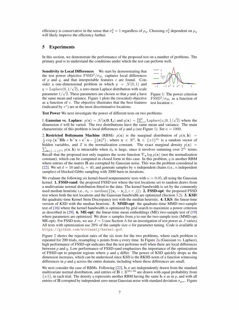
Figure 1: The power criterionFSSD2/σH1
as a function oftest location v.
Sensitivity to Local Differences We start by demonstrating thatthe test power objective FSSD2/σH1
captures local differencesof p and q, and that interpretable features v are found. Con-sider a one-dimensional problem in which p = N (0, 1) andq = Laplace(0, 1/
√2), a zero-mean Laplace distribution with scale
parameter 1/√
2. These parameters are chosen so that p and q havethe same mean and variance. Figure 1 plots the (rescaled) objectiveas a function of v. The objective illustrates that the best features(indicated by v∗) are at the most discriminative locations.
Test Power We next investigate the power of different tests on two problems:
1. Gaussian vs. Laplace: p(x) = N (x|0, Id) and q(x) =∏di=1 Laplace(xi|0, 1/
√2) where the
dimension d will be varied. The two distributions have the same mean and variance. The maincharacteristic of this problem is local differences of p and q (see Figure 1). Set n = 1000.
2. Restricted Boltzmann Machine (RBM): p(x) is the marginal distribution of p(x,h) =1Z exp
(x>Bh + b>x + c>x− 1
2‖x‖2), where x ∈ Rd, h ∈ {±1}dh is a random vector of
hidden variables, and Z is the normalization constant. The exact marginal density p(x) =∑h∈{−1,1}dh p(x,h) is intractable when dh is large, since it involves summing over 2dh terms.
Recall that the proposed test only requires the score function ∇x log p(x) (not the normalizationconstant), which can be computed in closed form in this case. In this problem, q is another RBMwhere entries of the matrix B are corrupted by Gaussian noise. This was the problem considered in[22]. We set d = 50 and dh = 40, and generate samples by n independent chains (i.e., n independentsamples) of blocked Gibbs sampling with 2000 burn-in iterations.
We evaluate the following six kernel-based nonparametric tests with α = 0.05, all using the Gaussiankernel. 1. FSSD-rand: the proposed FSSD test where the test locations set to random draws froma multivariate normal distribution fitted to the data. The kernel bandwidth is set by the commonlyused median heuristic i.e., σk = median({‖xi − xj‖, i < j}). 2. FSSD-opt: the proposed FSSDtest where both the test locations and the Gaussian bandwidth are optimized (Section 3.2). 3. KSD:the quadratic-time Kernel Stein Discrepancy test with the median heuristic. 4. LKS: the linear-timeversion of KSD with the median heuristic. 5. MMD-opt: the quadratic-time MMD two-sampletest of [16] where the kernel bandwidth is optimized by grid search to maximize a power criterionas described in [29]. 6. ME-opt: the linear-time mean embeddings (ME) two-sample test of [19]where parameters are optimized. We draw n samples from p to run the two-sample tests (MMD-opt,ME-opt). For FSSD tests, we use J = 5 (see Section A for an investigation of test power as J varies).All tests with optimization use 20% of the sample size n for parameter tuning. Code is available athttps://github.com/wittawatj/kernel-gof.
Figure 2 shows the rejection rates of the six tests for the two problems, where each problem isrepeated for 200 trials, resampling n points from q every time. In Figure 2a (Gaussian vs. Laplace),high performance of FSSD-opt indicates that the test performs well when there are local differencesbetween p and q. Low performance of FSSD-rand emphasizes the importance of the optimizationof FSSD-opt to pinpoint regions where p and q differ. The power of KSD quickly drops as thedimension increases, which can be understood since KSD is the RKHS norm of a function witnessingdifferences in p and q across the entire domain, including where these differences are small.
We next consider the case of RBMs. Following [22], b, c are independently drawn from the standardmultivariate normal distribution, and entries of B ∈ R50×40 are drawn with equal probability from{±1}, in each trial. The density q represents another RBM having the same b, c as in p, and with allentries of B corrupted by independent zero-mean Gaussian noise with standard deviation σper. Figure
7

0.00 0.02 0.04 0.06Perturbation SD σper
0.0
0.5
1.0
Rej
ecti
onra
te
FSSD-opt FSSD-rand KSD LKS MMD-opt ME-opt
1 5 10 15dimension d
0.0
0.5
1.0
Rej
ecti
onra
te
(a) Gaussian vs. Laplace.n = 1000.
0.00 0.02 0.04 0.06Perturbation SD σper
0.0
0.5
1.0
Rej
ecti
onra
te
(b) RBM. n = 1000. Per-turb all entries of B.
2000 4000Sample size n
0.00
0.25
0.50
0.75
Rej
ecti
onra
te
(c) RBM. σper = 0.1. Per-turb B1,1.
1000 2000 3000 4000Sample size n
0
100
200
300
Tim
e(s
)
(d) Runtime (RBM)
Figure 2: Rejection rates of the six tests. The proposed linear-time FSSD-opt has a comparable orhigher test power in some cases than the quadratic-time KSD test.
2b shows the test powers as σper increases, for a fixed sample size n = 1000. We observe that all thetests have correct false positive rates (type-I errors) at roughly α = 0.05 when there is no perturbationnoise. In particular, the optimization in FSSD-opt does not increase false positive rate when H0 holds.We see that the performance of the proposed FSSD-opt matches that of the quadratic-time KSD atall noise levels. MMD-opt and ME-opt perform far worse than the goodness-of-fit tests when thedifference in p and q is small (σper is low), since these tests simply represent p using samples, and donot take advantage of its structure.
The advantage of having O(n) runtime can be clearly seen when the problem is much harder,requiring larger sample sizes to tackle. Consider a similar problem on RBMs in which the parameterB ∈ R50×40 in q is given by that of p, where only the first entry B1,1 is perturbed by randomN (0, 0.12) noise. The results are shown in Figure 2c where the sample size n is varied. We observethat the two two-sample tests fail to detect this subtle difference even with large sample size. Thetest powers of KSD and FSSD-opt are comparable when n is relatively small. It appears that KSDhas higher test power than FSSD-opt in this case for large n. However, this moderate gain in the testpower comes with an order of magnitude more computation. As shown in Figure 2d, the runtimeof the KSD is much larger than that of FSSD-opt, especially at large n. In these problems, theperformance of the new test (even without optimization) far exceeds that of the LKS test. Furthersimulation results can be found in Section B.
(a) p = 2-component GMM.
−0.08
−0.04
0.00
0.04
0.08
0.12
0.16
0.20
(b) p = 10-component GMM
Figure 3: Plots of the optimization objective as a function oftest location v ∈ R2 in the Gaussian mixture model (GMM)evaluation task.
Interpretable Features In thefinal simulation, we demonstratethat the learned test locations areinformative in visualising wherethe model does not fit the datawell. We consider crime datafrom the Chicago Police Depart-ment, recording n = 11957locations (latitude-longitude co-ordinates) of robbery events inChicago in 2016.3 We addressthe situation in which a model pfor the robbery location density isgiven, and we wish to visualisewhere it fails to match the data. We fit a Gaussian mixture model (GMM) with the expectation-maximization algorithm to a subsample of 5500 points. We then test the model on a held-out test setof the same size to obtain proposed locations of relevant features v. Figure 3a shows the test robberylocations in purple, the model with two Gaussian components in wireframe, and the optimizationobjective for v as a grayscale contour plot (a red star indicates the maximum). We observe that the2-component model is a poor fit to the data, particularly in the right tail areas of the data, as indicatedin dark gray (i.e., the objective is high). Figure 3b shows a similar plot with a 10-component GMM.The additional components appear to have eliminated some mismatch in the right tail, however adiscrepancy still exists in the left region. Here, the data have a sharp boundary on the right sidefollowing the geography of Chicago, and do not exhibit exponentially decaying Gaussian-like tails.We note that tests based on a learned feature located at the maximum both correctly reject H0.
3Data can be found at https://data.cityofchicago.org.
8

Acknowledgement
WJ, WX, and AG thank the Gatsby Charitable Foundation for the financial support. ZSz wasfinancially supported by the Data Science Initiative. KF has been supported by KAKENHI InnovativeAreas 25120012.
References[1] R. R. Bahadur. Stochastic comparison of tests. The Annals of Mathematical Statistics, 31(2):
276–295, 1960.[2] L. Baringhaus and N. Henze. A consistent test for multivariate normality based on the empirical
characteristic function. Metrika, 35:339–348, 1988.[3] J. Beirlant, L. Györfi, and G. Lugosi. On the asymptotic normality of the l1- and l2-errors in
histogram density estimation. Canadian Journal of Statistics, 22:309–318, 1994.[4] R. Bhatia. Matrix analysis, volume 169. Springer Science & Business Media, 2013.[5] A. Bowman and P. Foster. Adaptive smoothing and density based tests of multivariate normality.
Journal of the American Statistical Association, 88:529–537, 1993.[6] C. Carmeli, E. De Vito, A. Toigo, and V. Umanità. Vector valued reproducing kernel Hilbert
spaces and universality. Analysis and Applications, 08(01):19–61, Jan. 2010.[7] K. Chwialkowski, D. Sejdinovic, and A. Gretton. A wild bootstrap for degenerate kernel tests. In
NIPS, pages 3608–3616, 2014.[8] K. Chwialkowski, A. Ramdas, D. Sejdinovic, and A. Gretton. Fast two-sample testing with
analytic representations of probability measures. In NIPS, pages 1981–1989, 2015.[9] K. Chwialkowski, H. Strathmann, and A. Gretton. A kernel test of goodness of fit. In ICML,
pages 2606–2615, 2016.[10] T. Epps and K. Singleton. An omnibus test for the two-sample problem using the empirical
characteristic function. Journal of Statistical Computation and Simulation, 26(3–4):177–203,1986.
[11] J. Frank J. Massey. The Kolmogorov-Smirnov test for goodness of fit. Journal of the AmericanStatistical Association, 46(253):68–78, 1951.
[12] L. J. Gleser. On a measure of test efficiency proposed by R. R. Bahadur. 35(4):1537–1544,1964.
[13] L. J. Gleser. The comparison of multivariate tests of hypothesis by means of Bahadur efficiency.28(2):157–174, 1966.
[14] J. Gorham and L. Mackey. Measuring sample quality with Stein’s method. In NIPS, pages226–234, 2015.
[15] J. Gorham and L. Mackey. Measuring sample quality with kernels. In ICML, pages 1292–1301.PMLR, 06–11 Aug 2017.
[16] A. Gretton, K. M. Borgwardt, M. J. Rasch, B. Schölkopf, and A. Smola. A kernel two-sampletest. JMLR, 13:723–773, 2012.
[17] A. Gretton, D. Sejdinovic, H. Strathmann, S. Balakrishnan, M. Pontil, K. Fukumizu, andB. K. Sriperumbudur. Optimal kernel choice for large-scale two-sample tests. In NIPS, pages1205–1213. 2012.
[18] L. Györfi and E. C. van der Meulen. A consistent goodness of fit test based on the total variationdistance. In G. Roussas, editor, Nonparametric Functional Estimation and Related Topics, pages631–645, 1990.
[19] W. Jitkrittum, Z. Szabó, K. P. Chwialkowski, and A. Gretton. Interpretable Distribution Featureswith Maximum Testing Power. In NIPS, pages 181–189. 2016.
[20] W. Jitkrittum, Z. Szabó, and A. Gretton. An adaptive test of independence with analytic kernelembeddings. In ICML, pages 1742–1751. PMLR, 2017.
[21] C. Ley, G. Reinert, and Y. Swan. Stein’s method for comparison of univariate distributions.Probability Surveys, 14:1–52, 2017.
9

[22] Q. Liu, J. Lee, and M. Jordan. A kernelized Stein discrepancy for goodness-of-fit tests. InICML, pages 276–284, 2016.
[23] J. Lloyd and Z. Ghahramani. Statistical model criticism using kernel two sample tests. In NIPS,pages 829–837, 2015.
[24] B. Mityagin. The Zero Set of a Real Analytic Function. Dec. 2015. arXiv: 1512.07276.[25] C. J. Oates, M. Girolami, and N. Chopin. Control functionals for Monte Carlo integration.
Journal of the Royal Statistical Society: Series B (Statistical Methodology), 79(3):695–718, 2017.[26] M. L. Rizzo. New goodness-of-fit tests for Pareto distributions. ASTIN Bulletin: Journal of the
International Association of Actuaries, 39(2):691–715, 2009.[27] R. J. Serfling. Approximation Theorems of Mathematical Statistics. John Wiley & Sons, 2009.[28] I. Steinwart and A. Christmann. Support Vector Machines. Springer, New York, 2008.[29] D. J. Sutherland, H.-Y. Tung, H. Strathmann, S. De, A. Ramdas, A. Smola, and A. Gretton.
Generative models and model criticism via optimized Maximum Mean Discrepancy. In ICLR,2016.
[30] G. J. Székely and M. L. Rizzo. A new test for multivariate normality. Journal of MultivariateAnalysis, 93(1):58–80, 2005.
[31] A. W. van der Vaart. Asymptotic Statistics. Cambridge University Press, 2000.[32] Q. Zhang, S. Filippi, A. Gretton, and D. Sejdinovic. Large-scale kernel methods for indepen-
dence testing. Statistics and Computing, pages 1–18, 2017.
10