Embed Size (px)
Citation preview
HAL Id: hal-00926822https://hal-supelec.archives-ouvertes.fr/hal-00926822
Submitted on 10 Jan 2014
HAL is a multi-disciplinary open accessarchive for the deposit and dissemination of sci-entific research documents, whether they are pub-lished or not. The documents may come fromteaching and research institutions in France orabroad, or from public or private research centers.
L’archive ouverte pluridisciplinaire HAL, estdestinée au dépôt et à la diffusion de documentsscientifiques de niveau recherche, publiés ou non,émanant des établissements d’enseignement et derecherche français ou étrangers, des laboratoirespublics ou privés.
Goal Tree Success Tree - Dynamic Master LogicDiagram and Monte Carlo Simulation for the Safety andResilience Assessment of a Multistate System of Systems
Elisa Ferrario, Enrico Zio
To cite this version:Elisa Ferrario, Enrico Zio. Goal Tree Success Tree - Dynamic Master Logic Diagram and Monte CarloSimulation for the Safety and Resilience Assessment of a Multistate System of Systems. EngineeringStructures, Elsevier, 2014, 59, pp.411-433. �10.1016/j.engstruct.2013.11.001�. �hal-00926822�

1
Goal Tree Success Tree - Dynamic Master Logic Diagram and Monte Carlo
Simulation for the Safety and Resilience Assessment of a Multistate System
of Systems
E. Ferrarioa and E. Zioa,b
aChair on Systems Science and the Energetic Challenge, European Foundation for New Energy - Electricité de
France, at École Centrale Paris - Supelec, France
[email protected], [email protected] bDepartment of Energy, Politecnico di Milano, Italy
Abstract
We extend a system-of-systems framework previously proposed by the authors to evaluate the
safety and physical resilience of a critical plant exposed to risk of external events. The
extension is based on a multistate representation of the different degrees of damage of the
individual components and the different degrees of safety of the critical plant. We resort to a
hierarchical model representation by Goal Tree Success Tree – Dynamic Master Logic
Diagram (GTST – DMLD), adapting it to the framework of analysis proposed. We perform
the quantitative evaluation of the model by Monte Carlo simulation. To the best of the
author’s knowledge this is the first time that a multistate framework of combined safety and
resilience analysis relating the structural and functional behaviour of the components to the
system function in a GTST – DMLD logic modelling of a system of systems is adopted in
Seismic Probabilistic Risk Assessment. To illustrate the approach, we adopt a case study that
considers the impacts produced by an earthquake and its aftershocks (the external events) on a
nuclear power plant (the critical plant) embedded in the connected power and water
distribution, and transportation networks which support its operation.
Keywords: Physical Resilience, Multistate Model, System of Systems, Goal Tree Success
Tree – Dynamic Master Logic Diagram, Monte Carlo simulation, Seismic Probabilistic Risk
Assessment.
2
1. INTRODUCTION
Resilience is the capacity of a system to survive to aggressions and shocks by changing its
non-essential attributes and rebuilding itself [1]; it includes technical, organizational, social
and economic facets [2]. In this work, we consider the “physical” resilience of a critical plant
exposed to risk of an external event. We limit the analysis to the capacity of recovering from
an external aggression or shock, using as representative quantity the recovery time, i.e., the
period necessary to restore a desired level of functionality of a system after the shock [2]. For
the resistance to the shock and the recovery from the shock, the critical plant is provided with
internal emergency devices (internal barriers) to keep it in, or restore it to, a safe state when
the main inputs devoted to this purpose fail. Since the internal emergency devices can fail too,
we extend the boundaries of the study to the infrastructure systems (external supports) in
which the plant is embedded, which also may or may not be left in the conditions to maintain
the safety of the plant after the occurrence of a disruptive event. Supporting elements (e.g.,
roads for access to the sites struck by the disruptive external event) are also considered for the
recovery of the failed components of the main inputs, internal barriers and external supports.
We adopt the system-of-systems framework of analysis proposed by the authors in [3] and
extend it to a multistate representation where different degrees of damage of the individual
components are contemplated [2], [4], [5]. In particular, we consider an original multistate
model of structural damage and functional performance at component level, that integrates
into a multistate model of safety at system level for well-being analysis [6].
The modelling of the system of systems includes: i) the connections among the main inputs ii)
the links among the internal barriers, iii) the dependencies among the external supports, iv)
the interdependencies between the systems in i), ii), iii), and the relationships among systems
in i), ii), iii) and the recovery supporting elements. We propose a hierarchical model
representation by Goal Tree Success Tree – Dynamic Master Logic Diagram (GTST-DMLD)
[7]. This provides an efficient and clear description of the system-of-systems complexity
through different hierarchical levels of system goals and functions, by the GT, and objects and
parts, by the ST. The interrelationships are represented in a DMLD that translates into a
dependency matrix and redefined logic gates, e.g., “AND” and “OR”, that assume a different
meaning with respect to a binary state model, e.g., Fault Tree [7]. We extend the GTST-
DMLD representation adapting it to the framework of analysis proposed. To the best of the
author’s knowledge this is the first time that a multistate framework of combined safety and
resilience analysis relating the structural and functional behaviour of the components to the

3
system function in a GTST – DMLD logic modelling of a system of systems is adopted in
Seismic Probabilistic Risk Assessment (SPRA). We use Monte Carlo simulation [8], [9], [10]
for the probabilistic evaluation of such system of systems considering multiple levels of safety
of the critical plant and physical resilience, measured in terms of the time needed to restore
the different levels of safety.
To illustrate the approach, we adopt a simplified case study that considers a nuclear power
plant (the critical plant) exposed to the risk of an earthquake and its subsequent aftershocks
(the external events). The plant is provided with proper internal emergency devices (internal
barriers), and embedded in the connected power and water distribution (external supports),
and transportation networks (recovery supporting elements) which support its operation and
provide resilience to it.
The reminder of the paper is organized as follows. In Section 2, the multistate model for the
safety assessment of a critical plant in a system-of-systems framework is presented; in Section
3, the Goal Tree Success Tree – Dynamic Master Logic Diagram and Monte Carlo simulation
are described in relation to Seismic Probabilistic Risk Assessment and within the multistate
system-of-systems framework; in Section 4, the case study and the results of the analysis are
presented; in Section 5, conclusions are provided. Finally, in Appendix A, an exemplification
of qualities, parts and GTST-DMLD within a system-of-systems framework is showed with
respect to Sections 2 and 3; in Appendix B, the basic concepts of a Seismic Probabilistic Risk
Assessment are introduced, to provide the reference elements needed for the case study; in
Appendix C, details of the operative steps of the GTST-DMLD and Monte Carlo simulation
for Seismic Probabilistic Risk Assessment are given.
2. MULTISTATE MODEL FOR THE SAFETY ASSESSMENT OF A
CRITICAL PLANT WITHIN A SYSTEM-OF-SYSTEMS
FRAMEWORK
In Section 2.1, the system-of-systems framework is illustrated with reference to three levels of
safety and distinguishing its goal and functions, i.e., its qualities, and its objects, i.e., its parts;
in Section 2.2, a multistate model for the system of systems is introduced.

4
2.1. System-of-systems framework: safety, qualities and parts
When due to an accident the main inputs to a critical plant stop, safety is assured by internal
barriers which provide the inputs in the amount necessary for the safety conditions. These
barriers are designed to withstand postulated accidents (design basis accidents) and include
multiple, independent and redundant layers of defense to compensate for potential human and
mechanical failures (defense in depth) [11]. As mentioned in the Introduction (Section 1), we
adopt a system-of-systems view [3] extending the analysis to the external supports for
emergency management actions and additional, redundant infrastructure systems to provide
the safety-required inputs in case of failure of both the main inputs and the first (internal)
barriers. In all generality, we consider also recovery supporting elements, as physical
components (e.g., roads for access to the site) and organizational elements (e.g., technical
competence of operators), that provide help in the recovery of the internal and external safety
systems. On the basis of this system-of-systems framework, we can identify three levels of
safety distinguishing the internal barriers (first level), the external supports (second level) and
the recovery supporting elements (third level), as illustrated in Figure 1.
Figure 1: Safety levels of a system-of-systems framework considering a critical plant in emergency conditions. The first level (top) considers internal barriers; the second one (middle) extends to the external supports; the
third one (bottom) accounts for the elements supporting the recovery.
In the present work, for the sake of simplicity, emergency management and organizational
supporting elements are not considered. The concept of resilience is limited to the physical
characteristics of the components and systems: then, we refer to physical resilience as the
underlying concept. On the other hand, the Goal Tree Success Tree Dynamic Master Logic
1st level
2nd level
3rd level
5
Diagram (GTST-DMLD) illustrated in Section 3 can accommodate elements of fuzzy logic
theory to describe imprecisely known characteristics and logic relations of non-physical facets
by linguistic fuzzy terms [7]. For example, specific inputs like the level of experience of the
operators can have an impact on the degree of safety of the critical plant in emergency
condition: these inputs could be described in the GTST-DMLD by including threshold values
[7]. This kind of considerations will be subject of further development in the future research.
In the framework under analysis, we can distinguish between qualities and parts. The former
are referred to the goals and functions, i.e., the objectives, of the system of systems; the latter
are related to the objects, i.e., the physical elements, that interact with each other to attain the
objectives.
In the following, we introduce a formal description of the qualities and parts, which can be
organized in hierarchies, with respect to a critical plant H whose state corresponds to the state
of its critical element, E.
The qualities are identified by the main goal F* concerning the safety of H, i.e., E, that is
attained by Fα, α = 1, …, N*, functions ordered in such a way that the first r directly achieve
the goal F* (i.e., they are principal functions) and the last N* – r support the first ones (i.e.,
they are auxiliary functions), as illustrated in Figure 2, on the left. The Fα, α = 1, …, N*,
functions may be hierarchically divided into other functions that can be further decomposed
into other ones until the required level of functional detail is reached. The last N* – r
functions are represented in a parallel branch of the same hierarchy of F* and they are
connected to it by a dashed line to highlight their auxiliary role.
The parts are composed by N infrastructure systems S(a), a = 1, …, A, divided in: nMI
infrastructure systems of main inputs, nIB internal barriers, nES external supports, nRS recovery
supporting elements (Figure 2, right). Each system S(a), a = 1, …, A, can be hierarchically
decomposed into other systems that can be in turn divided into other ones until the desired
level of detail of system components is reached. Some of the nMI, nIB and nES systems directly
provide necessary supplies to the critical element E (i.e., they are principal systems), whereas
some others among them are needed for the operation of the principal systems (i.e., they are
auxiliary systems); to point out the different role of the last ones, they are connected to the
corresponding principal systems by a dashed line (Figure 2, right), as for the functional
hierarchy. The nRS recovery supporting elements are considered apart from the other nMI, nIB
and nES systems since they are involved in the recovery of system safety.

6
Figure 2: Scheme of the hierarchies of the qualities (left) and parts (right) of a system of systems. The auxiliary functions and parts are connected by a dashed line to the hierarchy branch that they support. The indices α, β, γ, a, b, c are used to indicate the systems/elements in the hierarchies; nMI, nIB, nES, nRS refer to the number of main
inputs, internal barriers, external supports and recovery supporting elements, respectively.
Notice that in a system-of-systems view only one main function (F* ) is analyzed, whereas
more than one physical systems, involved in achieving that function, are considered (S(a), a =
1, …, A).
For illustration purpose, refer to Appendix A where an exemplification of qualities and parts
is given.
2.2. System-of-systems framework: multistate model
The safety assessment of the critical plant is based on multistate modeling. In particular, at
component level two aspects are described by the model: structural damage and functionality
(Section 2.2.1); at system-of-systems level, only functionality, which is based on the
structural and functional states of the components, is considered (Section 2.2.2).
2.2.1. Multistate model at component level: structural damage and functionality
Let us denote as η, η = 1, …, L, the generic component in the last level of the physical
hierarchies of the systems, S(a), a = 1, …, A, where L is the total number of components that
are not further decomposed. A disruptive external event can affect both the physical structure
and the functional performance of the generic component η, but not necessarily with a one-to-
one correspondence. For example, a road can be affected at different levels of damage by an
external event: from no damage to slight (few inches), moderate (several inches) or major
(few feet) settlements of the ground. When the road is slightly damaged it can still perform its
function (of connection) as in normal condition because the damage is negligible: then, the
functional performance associated to the structural states “no damage” and “slightly damage”

7
is the same. On the other hand, the correspondence between structural and functional states
strongly depends on their definition and on the scope of the application, e.g., in a
transportation planning the function of the road can be related to the traffic flow per hour and
in this case the performance may be reduced even for slight settlements of the ground due to a
decreasing speed of the vehicles, leading to a one-to-one correspondence between structural
and functional states.
We define as giη, i = 1, 2, …, G, and zj
η, j = 1, 2, …, Z, the structural and functional states of
the generic component η, respectively, where the indices i and j are ordered such that when i,j
= 1, the component is fully damaged and cannot perform its function (worst condition); when
i = G and j = Z, the component shows no damage and can fully perform its function (best
condition). Relations exist among the structural and functional states: a structural state
corresponds to one functional state but one functional state can be associated to one or more
structural states (Figure 3).
The evaluation of the safety of the critical plant is based on the functional state of the
components that in turn depends on their structural state. The analysis of the functional state
could be enough for evaluating the safety of the critical plant in the case of one-to-one
correspondence between structural and functional states. One the contrary, considering more
structural states than functional states allows us taking into account hidden (structural)
criticalities that can suddenly turn the functionality of a component into a worse state, e.g.,
upon occurrence of aftershocks. In fact, a same functional state can be reached from different
structural states, i.e., from different degrees of damage: even if functional performance is the
same, a component with worse structural state is more fragile if exposed to other external
events that can further degrade it structurally and at the same time cause a reduction of its
functionality. For example, with respect to Figure 3, it can be seen that the functional state zjη,
j = 3, can be reached when the component η is in the structural state giη, i = 4, i = 5 or i = 6,
but in the case i = 4 the component is weaker to withstand subsequent stresses than in the case
i = 6, and therefore it is more inclined to pass into a lower structural state, i.e., if the structural
state is lower than 4 (giη, i < 4), the functionality will be lower than 3 (zj
η, j < 3). With respect
to the example of the road above, when the road is slightly damaged it is more exposed to
aftershocks than when it is not damaged.

8
Figure 3: Relations between the structural, giη, i = 1, 2, …, G, and functional zj
η, j = 1, 2, …, Z, states for a component η.
In the case study exemplification of this work, we consider three structural and functional
states, i.e., giη and zj
η with i,j = 1, 2, 3. They represent risk, marginal and healthy conditions,
adopting the scheme of well-being analysis [6]. Denoting as yη,min the lowest output value that
it is requested by a component η to keep a safe state (it represents the risk threshold) and yη,opt
the optimal output value that should be provided by the component η to keep a safe state with
a safety margin, sm, (sm = yη,opt - yη,min), we define:
1. Risk state:
• Structural (giη, i = 1): the component η is strongly damaged by the external
event.
• Functional (zjη, j = 1): the component η cannot fulfill its function; its output yη
is lower than the minimal requested yη,min, i.e., yη < yη,min.
2. Marginal state:
• Structural (giη, i = 2): the component η is slightly damaged by the external
event.
• Functional (zjη, j = 2): the component η can fulfill its function, providing an
output yη that is lower than the optimal output yη,opt, but higher than the
minimal requested, i.e., yη,min ≤ yη < yη,opt, the safety margin is not satisfied.
3. Healthy state:
• Structural (giη, i = 3): the component is not damaged by the external event.
• Functional (zjη, j = 3): the component can fulfill its function, providing an
output yη that is equal or higher than the optimal output yη,opt, i.e., yη ≥ yopt.
9
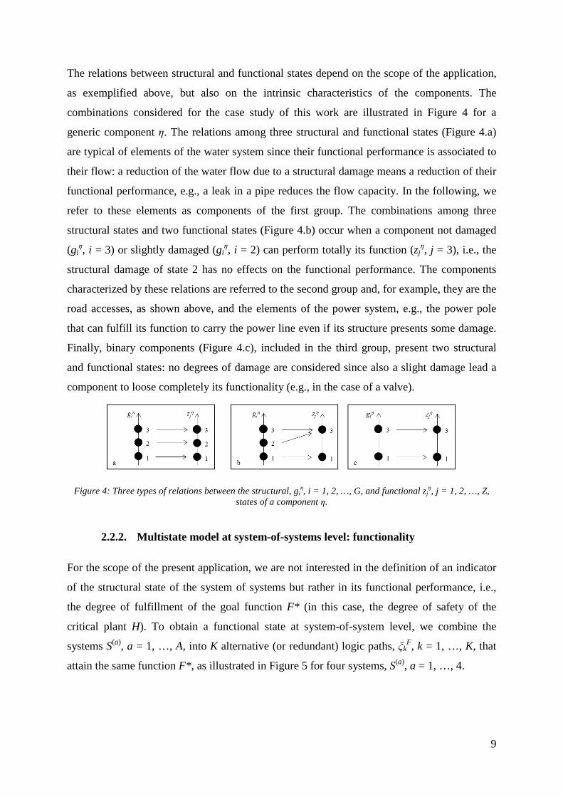
The relations between structural and functional states depend on the scope of the application,
as exemplified above, but also on the intrinsic characteristics of the components. The
combinations considered for the case study of this work are illustrated in Figure 4 for a
generic component η. The relations among three structural and functional states (Figure 4.a)
are typical of elements of the water system since their functional performance is associated to
their flow: a reduction of the water flow due to a structural damage means a reduction of their
functional performance, e.g., a leak in a pipe reduces the flow capacity. In the following, we
refer to these elements as components of the first group. The combinations among three
structural states and two functional states (Figure 4.b) occur when a component not damaged
(giη, i = 3) or slightly damaged (gi
η, i = 2) can perform totally its function (zjη, j = 3), i.e., the
structural damage of state 2 has no effects on the functional performance. The components
characterized by these relations are referred to the second group and, for example, they are the
road accesses, as shown above, and the elements of the power system, e.g., the power pole
that can fulfill its function to carry the power line even if its structure presents some damage.
Finally, binary components (Figure 4.c), included in the third group, present two structural
and functional states: no degrees of damage are considered since also a slight damage lead a
component to loose completely its functionality (e.g., in the case of a valve).
Figure 4: Three types of relations between the structural, giη, i = 1, 2, …, G, and functional zj
η, j = 1, 2, …, Z, states of a component η.
2.2.2. Multistate model at system-of-systems level: functionality
For the scope of the present application, we are not interested in the definition of an indicator
of the structural state of the system of systems but rather in its functional performance, i.e.,
the degree of fulfillment of the goal function F* (in this case, the degree of safety of the
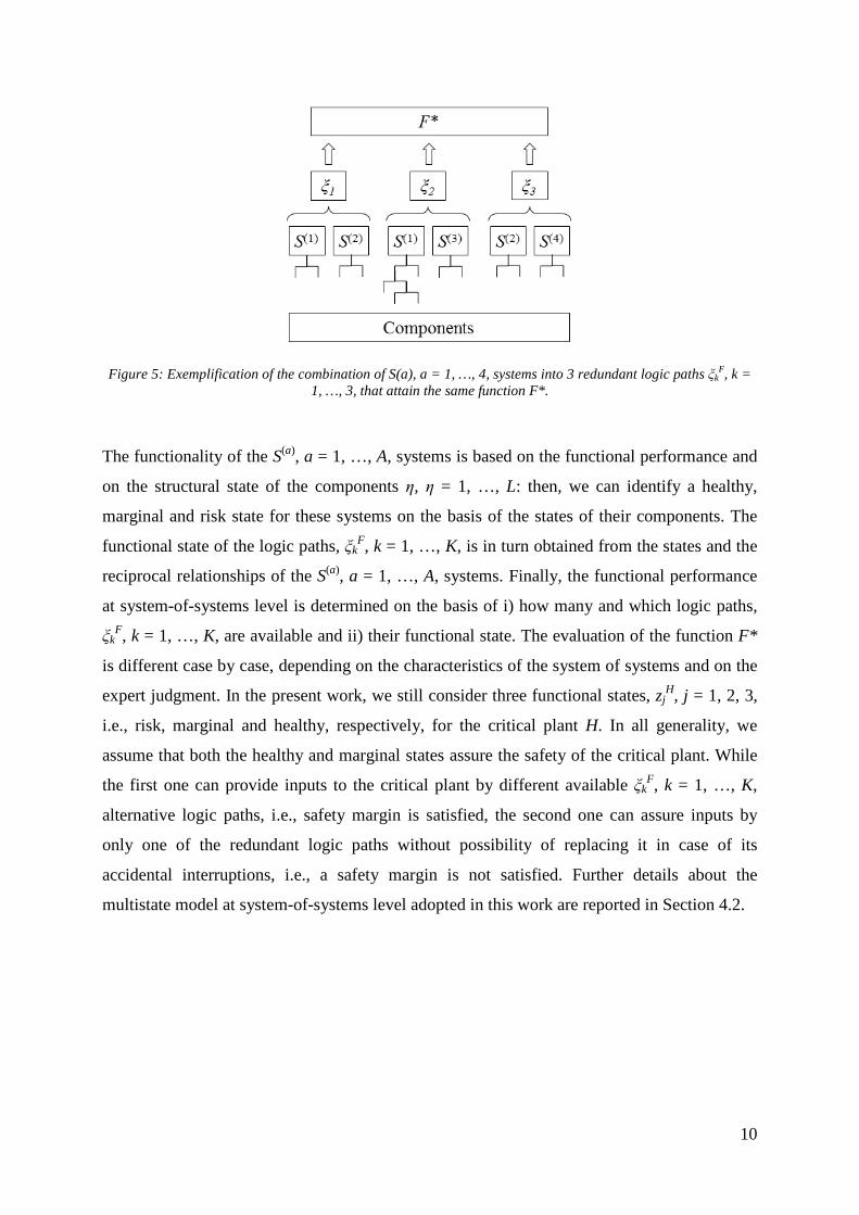
critical plant H). To obtain a functional state at system-of-system level, we combine the
systems S(a), a = 1, …, A, into K alternative (or redundant) logic paths, ξkF, k = 1, …, K, that
attain the same function F* , as illustrated in Figure 5 for four systems, S(a), a = 1, …, 4.
10
Figure 5: Exemplification of the combination of S(a), a = 1, …, 4, systems into 3 redundant logic paths ξkF, k =
1, …, 3, that attain the same function F*.
The functionality of the S(a), a = 1, …, A, systems is based on the functional performance and
on the structural state of the components η, η = 1, …, L: then, we can identify a healthy,
marginal and risk state for these systems on the basis of the states of their components. The
functional state of the logic paths, ξkF, k = 1, …, K, is in turn obtained from the states and the
reciprocal relationships of the S(a), a = 1, …, A, systems. Finally, the functional performance
at system-of-systems level is determined on the basis of i) how many and which logic paths,
ξkF, k = 1, …, K, are available and ii) their functional state. The evaluation of the function F*
is different case by case, depending on the characteristics of the system of systems and on the
expert judgment. In the present work, we still consider three functional states, zjH, j = 1, 2, 3,
i.e., risk, marginal and healthy, respectively, for the critical plant H. In all generality, we
assume that both the healthy and marginal states assure the safety of the critical plant. While
the first one can provide inputs to the critical plant by different available ξkF, k = 1, …, K,
alternative logic paths, i.e., safety margin is satisfied, the second one can assure inputs by
only one of the redundant logic paths without possibility of replacing it in case of its
accidental interruptions, i.e., a safety margin is not satisfied. Further details about the
multistate model at system-of-systems level adopted in this work are reported in Section 4.2.

11
3. GOAL TREE SUCCESS TREE – DYNAMIC MASTER LOGIC
DIAGRAM AND MONTE CARLO SIMULATION FOR SEISMIC
PROBABILISTIC RISK ASSESSMENT WITHIN A MULTISTATE
SYSTEM-OF-SYSTEMS FRAMEWORK
3.1. Goal Tree Success Tree - Dynamic Master Logic Diagram
The Goal Tree Success Tree – Dynamic Master Logic Diagram (GTST-DMLD) is a goal-
oriented method based on a hierarchical framework [7]. It gives a comprehensive knowledge
of the system describing the complex physical systems in terms of functions (qualities),
objects (parts) and their relationships (interactions). The first part is developed by the Goal
Tree (GT), the second one by the Success Tree (ST) and the third one by the DMLD [7].
The GT identifies the hierarchy of the qualities of the system decomposing the objective of
the analysis, i.e., the goal, into functions that are in turn divided into other functions and so on
by answering the question “how” they can attain the parent function (looking from top to
bottom of the hierarchy) and “why” the functions are needed (looking from bottom to top of
the hierarchy). Two types of qualities, i.e., main and support functions, are considered on the
basis of their role: the first ones are directly involved in achieving the goal, whereas, the
second ones are needed to support and realize the main functions [12]. For example, the goal
function of safely generating electric power in a nuclear power plant is attained by many
functions as heat generation, heat transport, emergency heat transport, heat to mechanical
energy transformation, mechanical to electrical energy transformation [13]. Each of these
functions require the support of other functions, e.g., emergency heat transport may require
internal cooling [13] or a pump whose function is to “provide pressure” require the support
functions “provide ac power”, “cooling and lubrication”, “activation and control” [13].
The ST represents the hierarchy of the objects of the system from the whole system to the
parts necessary to attain the last levels of the GT. This hierarchy is built identifying the
elements that are “part of” the parent objects. As for the GT, two types of objects are
distinguished: main and support objects. The first ones are directly needed to achieve the main
functions, whereas the second ones are needed for the operation of the main objects [12]. For
example, generating power plants, electric power transmission and distribution networks are
the support objects to provide ac power to a pump.
12
The DMLD is an extension of the Master Logic Diagram (MLD) [7] to model the dynamic
behavior of a physical system. It identifies the interactions between parts, functions and parts
and functions, in the form of a dependency matrix and it adds the dynamic aspect by
introducing time-dependent fuzzy logic [7].
Further details are not given here for brevity sake: the interested reader is referred to the cited
literature [12], [7]. In the next Section, the adaption of the GTST-DMLD for a multistate
system-of-systems framework is illustrated.
3.2. Goal Tree Success Tree - Dynamic Master Logic Diagram of a system of systems
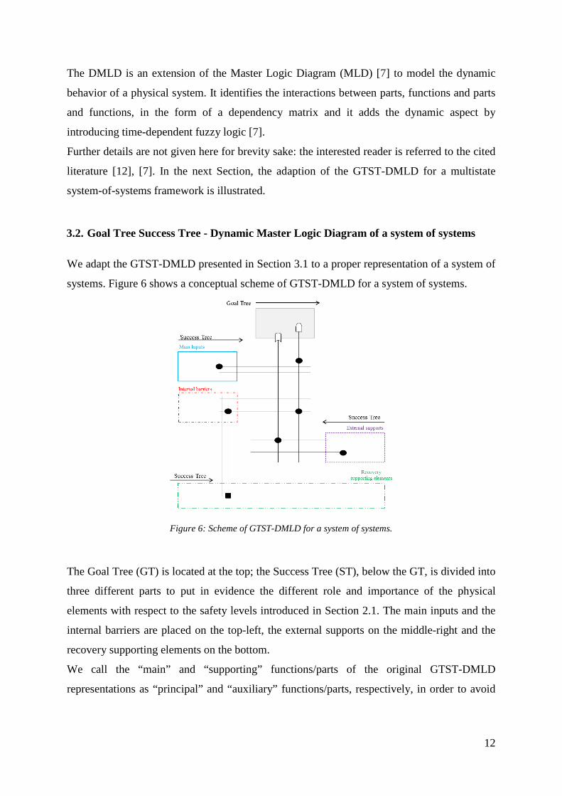
We adapt the GTST-DMLD presented in Section 3.1 to a proper representation of a system of
systems. Figure 6 shows a conceptual scheme of GTST-DMLD for a system of systems.
Figure 6: Scheme of GTST-DMLD for a system of systems.
The Goal Tree (GT) is located at the top; the Success Tree (ST), below the GT, is divided into
three different parts to put in evidence the different role and importance of the physical
elements with respect to the safety levels introduced in Section 2.1. The main inputs and the
internal barriers are placed on the top-left, the external supports on the middle-right and the
recovery supporting elements on the bottom.
We call the “main” and “supporting” functions/parts of the original GTST-DMLD
representations as “principal” and “auxiliary” functions/parts, respectively, in order to avoid

13
confusion with the main inputs, the external supports and the recovery supporting elements of
the system-of-systems framework.
The relationships among elements and functions are illustrated by the MLD. In particular, the
connections among components of i) the main inputs, ii) the internal barriers, iii) the external
supports are shown; the interdependencies between the systems i), ii), iii) are depicted; the
links of the recovery supporting elements with the systems i), ii), iii) are indicated; the
connections between the systems i), ii), iii) and the functions of the Goal Tree are given. Two
types of dependencies have been taken into account: direct and support dependencies. The
first ones, identified by a dot in the representation and called in the following “dot-
dependencies”, express the need to have the element on the bottom in operation to achieve
(with respect to a function) or to let working (with respect to an object) the element on the
top. The support dependencies, depicted by a square and called hereafter “square-
dependencies”, mean that the element on the bottom is needed for the recovery of the element
on the top: its failure does not cause the failure of the corresponding elements, but it increases
the recovery time of the connected element in the case that this fails too. It acts like a delay in
the repairing of the connected components. Thus, the square-dependencies are “time
dependent”: when a component does not need recovery they can be neglected, whereas, in the
opposite case, they become fundamental until the complete restoration of the component; at
this point, they can be neglected again. They are key elements of the model for the evolution
in time of the recovery process and they can modify (increase) the total recovery time of the
component that needs to be restored.
The dynamic aspect, consisting in the functional multistate of the components, is represented
by the logic gates “AND” and “OR” that assume the same meaning as in [7] to evaluate the
state of the connected components and functions from the bottom to the top of the diagram:
the minimum and the maximum values of inputs are the output values in case of “AND” and
“OR” gates, respectively. In this state analysis only the dot-dependencies are considered. In
the present work the inputs are discrete states (see Section 2.2) but are not described by fuzzy
intervals as in [7].
On the contrary, in the evaluation of the physical resilience both the dot- and square-
dependencies are included and the logic gates “AND” and “OR” have an opposite meaning
with respect to the state evaluation. In fact, the output values of the “OR” and “AND” gates
are the minimum and the maximum values of the inputs, respectively. In this case, the inputs
are the recovery time values. For example, refer to Figure 7 where two systems S(a), a = 1, 2,
contribute to the realization of the function F* (dot-dependencies) and two other systems S(a),

14
a = 3, 4, are relevant only to allow the recovery of the system S(a), a = 2, (square-
dependencies). Assuming that S(1) and S(4) are in functional state 3, zjS(1) and zj
S(4), j = 3, with
associated recovery time (RTS(1) and RTS(4)) equal to 0, and S(2) and S(3) are in state 1, zjS(2) and
zjS(3), j = 1, with associated recovery times (RTS(2) and RTS(3)) equal to 2 and 5, respectively,
the function F* is in state 1, zjF*, j = 1, since the “AND” gate (G1) means “minimum values
between zjS(1) and zj
S(2)”. The time needed to realize the function F* is 7 (RTF* = 7) since the
“AND” gate (G1) means “maximum values between RTS(1) and RTS(2)”, where the total time
needed to recover S(2) depends on the time to recover S(2) itself and the maximum value
(“AND” gate G2) between RTS(3) and RTS(4). Replacing the “AND” gate G2 with an “OR”
gate, the total time needed to recover S(2) is 2, since the minimum value between RTS(3) and
RTS(4) is zero. Replacing both the “AND” gates, G1 and G2, with two “OR gates, the function
F* is in state 3, zjF*, j = 3, thus, it is not necessary to recover it (RTF* = 0).
Figure 7: Example of the use of the “AND” logic gate together with the dot- and square- dependencies for computing the state and the recovery time of the function F*.
In Appendix A, an example of GTST-DMLD is reported.
3.3. Monte Carlo simulation for Seismic Probabilistic Risk Assessment within a system-
of-systems framework
Within the system-of-systems analysis framework here purported, in the case study of the
next Section 4 we wish to evaluate the safety of the critical plant H (a nuclear power plant)
exposed to the risk from earthquakes and aftershocks occurrence (see Appendix B),
accounting for the structural and functional responses of the systems inside and outside the
plant, i.e., main inputs, internal barriers, external supports and recovery supporting elements,
through the analysis of the underlying dependency structure. In addition, we wish to

15
determine the physical resilience of the system of systems, evaluated in terms of the time of
recovery of safety states 2 and 3 (marginal and healthy, respectively) of the critical plant. To
do this, we adopt the GTST-DMLD representation of the system of systems and Monte Carlo
(MC) simulation for the quantitative SPRA evaluation [14]. The simulation procedure is
illustrated in Appendix C.
4. CASE STUDY
We recall the case study of [3] concerning the safety of a nuclear power plant (the critical
plant), in response to an earthquake (the external hazardous event). The problem is analyzed
in a system-of-systems framework, distinguishing main inputs, internal barriers, external
supports and recovery supporting elements. We adopt a multistate model to identify different
degrees of component damage and, consequently, different degrees of system safety. In
particular, at the system level we consider three states of the nuclear power plant of which two
correspond to safe conditions (marginal and healthy, see Section 2.2). Safe condition means
that the nuclear power plant does not cause health problems and environmental damages, i.e.,
it does not release radioactive material to the environment. To maintain these conditions it
must be provided with energy and water flow inputs to absorb the heat that it generates.
We analyze also the physical resilience of the system of systems, in terms of the time
necessary to recover the safe states (marginal and healthy) of the plant including the
occurrence of aftershocks that can further degrade the system of systems.
When an earthquake occurs, the critical plant may not receive the input necessary to be kept
in, or restored to, a safe state due to the direct impact on its emergency devices and to the
damage to the interconnected infrastructures. Two quantities are used to characterize the loss
of functionality of the various components of the system of systems embedding the critical
plant, upon the occurrence of a damaging external event:
- from the safety viewpoint, the probability that the critical plant remains in marginal
and healthy states;
- from the physical resilience viewpoint, the time needed to recover the marginal and
healthy states of the critical plant facing the occurrence of aftershocks.
Both quantities are here computed for an earthquake of magnitude equal to 5.5 on the moment
magnitude scale.
In Section 4.1, the description of the system studied is given under a number of assumptions
which simplify the problem to the level needed to convey the key aspects of the conceptual

16
system-of-systems framework, while maintaining generality. In Section 4.2, the Goal Tree
Success Tree – Dynamic Master Logic Diagram representation of the system-of-systems
considered in the case study is given. In Section 4.3, we provide the results of the evaluation
of the two quantities of interest above mentioned.
4.1. Description of the system of systems
The critical plant, i.e., the nuclear power plant (NPP), is composed by a Main Feedwater
(MFW) system that provides coolant useful to absorb the heat generated and four internal
barriers: High Pressure Coolant Injection (HPCI) and Low Pressure Coolant Injection (LPCI)
systems that provide water to cool the reactor, an automatic depressurization system (ADS)
that reduces the pressure in the reactor vessel and a diesel generator (DG) that can provide the
LPCI system with power.
The MFW system is formed by a condenser where the unused steam coming from a turbine is
condensed into water that is pumped to the reactor vessel by the feedwater pump (FWP) and
pipes (Pi1 and Pi2). In case of accident damaging the MFW system function, the HPCI and
LPCI systems need to provide the necessary function. Both systems are composed by a
condensate storage tank (CST1 and CST2, respectively), a pump (HPP and LPP, respectively)
and pipes (Pi3, Pi4 and Pi5, Pi6, respectively). To operate, the LPCI system needs the
automatic depressurization system (ADS) to reduce the pressure inside the vessel. Apart from
the pump of the HPCI system that is a turbine-driven pump, the pumps of the MFW and LPCI
systems need electrical power to work. This is usually provided by the offsite power and in
case of its loss, the emergency diesel generator can be activated to supply the LPP.
The external supports of the critical plant are the offsite power system (EE) and an external
water (EW) system. The first one is composed by a generation station (GS) that produces the
electrical energy, a substation (S) that transforms the voltage from high to low, power lines
and poles (Po1 and Po2) to support them. The second one is formed by the river, i.e., the
source of water, a pump (RP) that receives electrical power from the offsite power system and
pipes (Pi7 and Pi8) that carry the water.
The recovery supporting elements are the road accesses to the components of the system of
systems. The state of the roads is important for access of materials and operators that are
needed to restore the components required for the safe state of the critical plant.
17
Actually, in view of the methodological character of this work, for the sake of simplicity,
power lines are not here considered and the assumption is made that the river is not perturbed
by the earthquake so that it is a source of water always available.
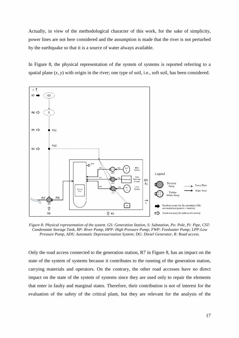
In Figure 8, the physical representation of the system of systems is reported referring to a
spatial plane (x, y) with origin in the river; one type of soil, i.e., soft soil, has been considered.
Figure 8: Physical representation of the system. GS: Generation Station, S: Substation, Po: Pole, Pi: Pipe, CST: Condenstate Storage Tank, RP: River Pump, HPP: High Pressure Pump; FWP: Feedwater Pump; LPP:Low
Pressure Pump, ADS: Automatic Depressurization System; DG: Diesel Generator, R: Road access.
Only the road access connected to the generation station, R7 in Figure 8, has an impact on the
state of the system of systems because it contributes to the running of the generation station,
carrying materials and operators. On the contrary, the other road accesses have no direct
impact on the state of the system of systems since they are used only to repair the elements
that enter in faulty and marginal states. Therefore, their contribution is not of interest for the
evaluation of the safety of the critical plant, but they are relevant for the analysis of the

18
physical resilience of the system of systems. Given the different role of the road access R7 we
will consider it, in the following, as an auxiliary element of the offsite power system.
Figure 9 represents the spatial localization of the system shown in Figure 8 with reference to
the reciprocal position of all the components (Figure 9, left) and to the position of the system
with respect to the considered earthquake epicenter A(70, 70) (Figure 9, right). The distances
on the axes are expressed in kilometers.
Figure 9: Left: spatial localization of the nuclear power plant (star) with respect to the components of the electric power system (circle, from top to bottom: Generation Station, Substation, Pole 1, Pole 2), water system (square, from left to right: River, Pipe 7, RP, Pipe 8) and road transportation (triangle, from top to bottom and
from left to right: R7, R6, R5, R4, R3, R2, R1). Right: spatial localization of the system of systems with respect to the earthquake’s epicenter A(70, 70).
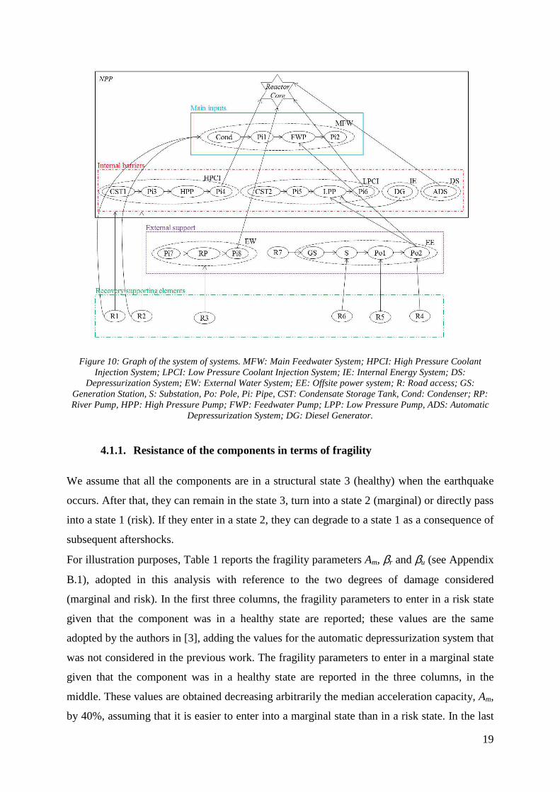
Figure 10 shows the graph of the system of systems with respect to the safety levels of
Section 2.1. The arrows are directed from one element to another one which depends on it.
-0.6 -0.5 -0.4 -0.3 -0.2 -0.1 0 0.1 0.2 0.3 0.4 0.5 0.6 0.7 0.8 0.9 11
0
2
4
6
8
10
12
14
16
-10 0 10 20 30 40 50 60 70 80 90 100-10
0
10
20
30
40
50
60
70
80
90
100
x [km]
y [k
m]
x [km]
y [k
m]
A
System of systems
19
Figure 10: Graph of the system of systems. MFW: Main Feedwater System; HPCI: High Pressure Coolant Injection System; LPCI: Low Pressure Coolant Injection System; IE: Internal Energy System; DS:
Depressurization System; EW: External Water System; EE: Offsite power system; R: Road access; GS: Generation Station, S: Substation, Po: Pole, Pi: Pipe, CST: Condensate Storage Tank, Cond: Condenser; RP: River Pump, HPP: High Pressure Pump; FWP: Feedwater Pump; LPP: Low Pressure Pump, ADS: Automatic
Depressurization System; DG: Diesel Generator.
4.1.1. Resistance of the components in terms of fragility
We assume that all the components are in a structural state 3 (healthy) when the earthquake
occurs. After that, they can remain in the state 3, turn into a state 2 (marginal) or directly pass
into a state 1 (risk). If they enter in a state 2, they can degrade to a state 1 as a consequence of
subsequent aftershocks.
For illustration purposes, Table 1 reports the fragility parameters Am, βr and βu (see Appendix
B.1), adopted in this analysis with reference to the two degrees of damage considered
(marginal and risk). In the first three columns, the fragility parameters to enter in a risk state
given that the component was in a healthy state are reported; these values are the same
adopted by the authors in [3], adding the values for the automatic depressurization system that
was not considered in the previous work. The fragility parameters to enter in a marginal state
given that the component was in a healthy state are reported in the three columns, in the
middle. These values are obtained decreasing arbitrarily the median acceleration capacity, Am,
by 40%, assuming that it is easier to enter into a marginal state than in a risk state. In the last

20
three columns, the fragility parameters to enter into a risk state given that the component was
in a marginal state are illustrated. These values are identified by decreasing the median
acceleration capacity, Am, of the healthy state by 55%, since a component in a marginal state
is more prone to pass into a risk state than a component in a healthy state. In Figure 11, the
fragility curves obtained by the parameters of Table 1 are depicted: the fragility curves of
exceeding a risk threshold given that the initial states were healthy and marginal are
illustrated in dashed and solid lines, respectively, the fragility curve of exceeding a marginal
threshold given that the initial state was healthy is represented in dotted line.
Table 1: Fragility parameters used in the present work with respect to the transitions healthy-risk, healthy-marginal and marginal-risk.
Healthy � Risk Healthy � Marginal Marginal � Risk
Am βr βu Am βr βu Am βr βu
Generation station 0.70 0.30 0.10 0.42 0.30 0.10 0.32 0.30 0.10 Substation 0.90 0.40 0.30 0.54 0.40 0.30 0.41 0.40 0.30 Power Pole 0.80 0.20 0.20 0.48 0.20 0.20 0.36 0.20 0.20 Diesel Generator 0.70 0.40 0.20 0.42 0.40 0.20 0.32 0.40 0.20 Pipe 1.88 0.43 0.48 1.13 0.43 0.48 0.85 0.43 0.48 Pump 0.20 0.20 0.30 0.12 0.20 0.30 0.09 0.20 0.30 Condensate storage tank / Condenser 0.20 0.10 0.10 0.12 0.10 0.10 0.09 0.10 0.10 Automatic depressurization system 1.5 0.3 0.3 - - - - - - Road 0.30 0.30 0.20 0.18 0.30 0.20 0.14 0.30 0.20

21
Figure 11: Fragility curves as a function of the peak ground acceleration (PGA) [m/s2] for the following components: Generation Station (GS), Substation (S), Power Pole (Po), Diesel Generator (DG), Automatic Depressurization System (ADS), Road Access (R), Condensate Storage Tank (CST), Condenser (Cond), Pump, Pipe (Pi). The fragility curves of exceeding a risk threshold given that the initial states were healthy and marginal are illustrated in dashed and solid lines, respectively, the fragility curve of exceeding a marginal threshold given that the initial state was healthy is represented in dotted line.
Notice that the automatic depressurization system presents fragility parameters only to enter
into a risk state from a healthy state, since we describe it with a binary state model: with
respect to the taxonomy of combinations of structural and functional states introduced in
Section 2.2.1, it belongs to the third group of components.
On the contrary, we consider the pumps and pipes in the first group (three structural and three
functional states) since their functional performance is associated to the water flow. For the
sake of simplicity, the condensate storage tank and the condenser are included in the second
group even if they concern the water flow. The elements of the power systems and the road
access belong to the second group too, since a slight damage in their parts does not affect their
functionality: a power pole can or cannot support the power lines, a generation station can or
0 0.5 1 1.5 20
0.2
0.4
0.6
0.8
1
PGA [m/s2]
Fra
gilit
y
GS
0 0.5 1 1.5 20
0.2
0.4
0.6
0.8
1
PGA [m/s2]
Fra
gilit
y
S
0 0.5 1 1.5 20
0.2
0.4
0.6
0.8
1
PGA [m/s2]
Fra
gilit
y
DG
0 0.5 1 1.5 20
0.2
0.4
0.6
0.8
1
PGA [m/s2]
Fra
gilit
y
ADS
0 0.5 1 1.5 20
0.2
0.4
0.6
0.8
1
PGA [m/s2]
Fra
gilit
y
CST/Cond
0 0.5 1 1.5 20
0.2
0.4
0.6
0.8
1
PGA [m/s2]
Fra
gilit
y
Pump
0 0.5 1 1.5 20
0.2
0.4
0.6
0.8
1
PGA [m/s2]
Fra
gilit
y
Po
0 0.5 1 1.5 20
0.2
0.4
0.6
0.8
1
PGA [m/s2]
Fra
gilit
y
R
0 0.5 1 1.5 20
0.2
0.4
0.6
0.8
1
PGA [m/s2]
Fra
gilit
y
Pi
22
cannot produce the quantity of energy requested, a road can or cannot provide access to the
connected component.
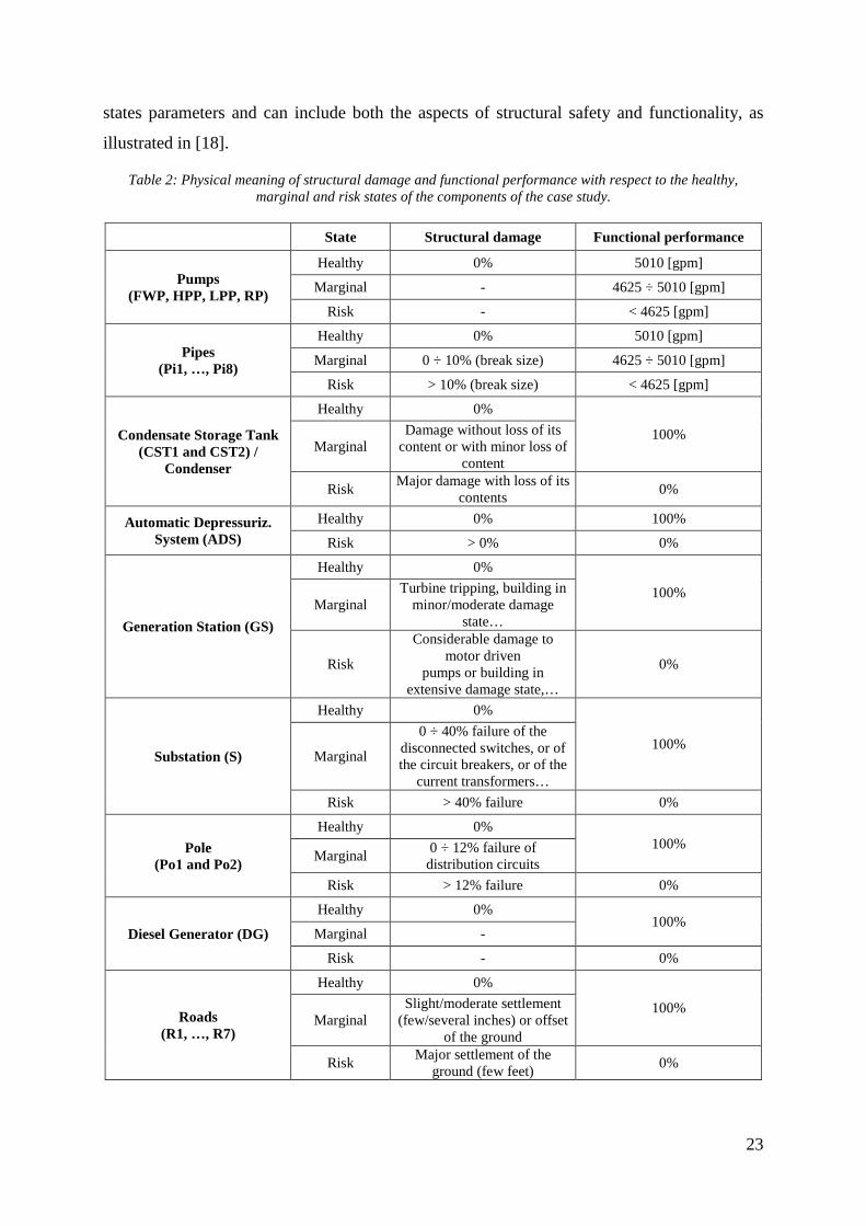
Table 2 reports examples of structural damage to show the meaning of a specific component
being in a healthy, marginal or risk states. These values have been extracted from [15] where
five levels of structural damage (none, slight/minor, moderate, extensive, complete) are
identified for some components of the power, water and transportation systems. For example,
for a substation a slight damage is defined as the failure of 5% of the disconnected switches,
or the failure of 5% of the circuit breakers, or by the building being in minor damage state; a
moderate damage is defined as the failure of 40% of the disconnected switches, or the failure
of 40% of the circuit breakers, or the failure of 40% of the current transformers, or by the
building being in moderate damage state; an extensive damage is defined as the failure of
70% of the disconnected switches, or the failure of 70% of the circuit breakers, or the failure
of 70% of the current transformers, or by the building being in extensive damage state; a
complete damage is defined as the failure of all disconnected switches, or the failure of all the
circuit breakers, or the failure of all the current transformers, or by the building being in
complete damage state [15]. In the Table, the values are grouped into the three structural
states: healthy (i.e., none damage) marginal (i.e., slight/minor and moderate) and risk (i.e.,
extensive and complete). The structural state for the pipes is taken from [16] that distinguish
between small (< 2%), intermediate (2% ÷ 10%) and large breaks (> 10%). Here it is
considered that the marginal state includes the small and intermediate breaks.
In Table 2, also the functional performance of a component that is in a specific state is
reported. Values of flow are identified for the components of the group 1; whereas
percentages of 100% or 0% of functionality are associated with the components of the groups
1 and 2 that have binary functional states. To identify the flow values, we consider that in
shutdown conditions the flow rate to cool the reactor is between 4625 gpm [16] and 5010 gpm
[17]. Therefore, a component of a water system of the group 3 is in a healthy functional state
if it can provide a quantity of water equal or higher than 5010 gpm, it is in a marginal
functional state if it can provide a quantity in the interval 4625 gpm - 5010 gpm, otherwise it
is in a risk functional state.
Note that, in this work we have not considered interdependence between structural and
functional thresholds since we have assumed that the functionality depends on the structural
state. A further study will be performed to identify the correspondence between structural and
functional state quantitatively, or to determine fragility curves that are based on multiple limit
23
states parameters and can include both the aspects of structural safety and functionality, as
illustrated in [18].
Table 2: Physical meaning of structural damage and functional performance with respect to the healthy, marginal and risk states of the components of the case study.
State Structural damage Functional performance
Pumps (FWP, HPP, LPP, RP)
Healthy 0% 5010 [gpm]
Marginal - 4625 ÷ 5010 [gpm]
Risk - < 4625 [gpm]
Pipes (Pi1, …, Pi8)
Healthy 0% 5010 [gpm]
Marginal 0 ÷ 10% (break size) 4625 ÷ 5010 [gpm]
Risk > 10% (break size) < 4625 [gpm]
Condensate Storage Tank (CST1 and CST2) /
Condenser
Healthy 0%
100% Marginal
Damage without loss of its content or with minor loss of
content
Risk Major damage with loss of its
contents 0%
Automatic Depressuriz. System (ADS)
Healthy 0% 100%
Risk > 0% 0%
Generation Station (GS)
Healthy 0%
100% Marginal
Turbine tripping, building in minor/moderate damage
state…
Risk
Considerable damage to motor driven
pumps or building in extensive damage state,…
0%
Substation (S)
Healthy 0%
100% Marginal
0 ÷ 40% failure of the disconnected switches, or of the circuit breakers, or of the
current transformers…
Risk > 40% failure 0%
Pole (Po1 and Po2)
Healthy 0% 100%
Marginal 0 ÷ 12% failure of distribution circuits
Risk > 12% failure 0%
Diesel Generator (DG)
Healthy 0% 100%
Marginal -
Risk - 0%
Roads (R1, …, R7)
Healthy 0%
100% Marginal
Slight/moderate settlement (few/several inches) or offset
of the ground
Risk Major settlement of the
ground (few feet) 0%
24
4.1.2. Physical resilience in terms of time of recovery
The physical resilience of the system of systems is quantified in terms of the time needed to
recover the healthy state of the critical plant starting from a risk and marginal state, and its
marginal state starting from a risk state. To compute this, the evolution in time of the system
of systems is included in the SPRA framework.
As illustrated in the procedure of Appendix C, the recovery time of the nuclear power plant is
computed starting from the recovery time of the individual components and analyzing the
dependency structure identified by the GTST-DMLD.
To account for the uncertainty in the duration of the recovery, lognormal distributions have
been associated to the recovery time of the individual components. Table 3 shows the means
and the error factors used in this study to recover the safety i) from risk to healthy state (first
two columns), ii) from marginal to healthy state (two columns in the middle) and iii) from risk
to marginal state (last two columns). The values of recovery from risk to healthy state are the
same used by the authors in [19] and they are based on the following consideration. The time
to recover a component depends on its size, its location, the type of damage and easiness to
locate the failure. It is assumed that the components inside the nuclear power plant need more
time for the recovery than the components outside. In particular, this happens when it is
necessary to replace part of the component or the entire component given its huge dimensions
and the difficulty to operate inside the plant. For this reason, we have assumed that the mean
of the time needed to recover the pump inside the nuclear power plant is larger than that
needed for the pump outside. The large mean value of the time to recover the condensate
storage tanks and condenser is due to their size, location inside the plant and difficulty in
restoration. The time to physically repair a pipe could be very short (even few hours), but we
have assumed a mean value equal to 4 days to account for the potential difficulty in locating
the break. The diesel generator has a time of repair with a high uncertainty (error factor equal
to 5), because it may vary significantly depending on the type of damage. The components
with lowest mean value of the recovery time are the power pole, the road, the generation
station and the substation that are outside the plant; the latter are affected by large uncertainty
(error factors of 5 and 10, respectively), because their recovery depends on the intensity of the
damage, e.g., a generation station can be slightly perturbed by the earthquake and its repairing
can last few hours but it can also be destroyed, and in this case the time to build it again is
obviously much higher. Finally, also the automatic depressurization system, even if inside the

25
plant, presents a short recovery time, because we assume that it is easy to replace it with
another one.
The mean values of recovery for the cases ii) and iii) above are identified by considering that
the time to recover a component from risk to marginal state is longer than that from marginal
to healthy state and their sum is equal to the direct recovery from risk to healthy state. Thus,
we define the mean values for the cases ii) and iii) as the 30% and 70%, respectively, of the
mean value from risk to healthy state.
Table 3: Mean, �, and Error Factor, EF, of the recovery time lognormal distribution used in the present work with respect to the transitions risk-healthy, marginal-healthy, risk-marginal.
Risk � Healthy Marginal � Healthy Risk � Marginal
� [days] EF � [days] EF � [days] EF
Generation station 1 10 0.3 10 0.7 10 Substation 1 5 0.3 5 0.7 5 Power Pole 1.5 3 0.45 3 1.05 3 Diesel Generator 30 5 9 5 21 5 Pipe 4 3 1.2 3 2.8 3 Pump (inside the plant) 75 3 22.5 3 52.5 3 Pump (outside the plant) 5 3 1.5 3 3.5 3 Condensate storage tank / Condenser 75 3 22.5 3 52.5 3 Automatic depressurization system 1 3 - - - - Road 2 3 0.6 3 1.4 3
4.2. GTST-DMLD and physical resilience of the system of systems
Figure 12 shows the GTST-DMLD of the system of systems depicted following the scheme of
Figure 6 and on the basis of the graph of Figure 10. The goal function is the safety of the
nuclear power plant assured by water inputs (i.e., the principal function) that can be provided
by four different alternative paths (ξkWater, k = 1, …, 4): the main feedwater system (ξ1
Water),
the high pressure coolant injection system (ξ2Water), the combination of low pressure coolant
injection and depressurization systems (ξ3Water), the external water system (ξ4
Water). The power
coming from outside (Ext) or inside (Int) the plant is an auxiliary function to support the
operation of most of the water systems. For the explanation of the logic gates, of dot- and
square- dependencies, see Section 3.2.
It can be seen that the components among the systems MFW, HPCI, LPCI, EW, EE are
connected in series for the presence of the “AND” gates. The systems IE, DS, R1, R2, R3, R4,
R5, R6 and R7 are composed by only one component. Finally, the systems EE and IE are in
26
parallel with respect to the LPCI system, as the roads R1 and R2 with reference to the
components inside the nuclear power plant (“OR” gates).
Following the rules of the “AND” and “OR” gates, it is possible to compute the state and the
mean time to recover the paths ξkWater, k = 1, …, 4, and, then, the safety and the recovery of
the nuclear power plant. For example, the mean time to recover ξkWater, k = 1, is the maximum
between the mean times to recover the MFW system and the EE system:
E[ξ1Water] = max(E[RTMFW], E[RTEE]),
where E[RTMFW] is the maximum expected value between the components of the MFW
system and the minimum expected value of the two road accesses connected to them, and
E[RTEE] is the maximum expected value between the components of the EE system and their
road accesses:
E[RTMFW] = max(E[RTPi2], E[RTFWP], E[RTPi1], E[RTCond], min(E[RTR1], E[RTR2]))
E[RTEE] = max(E[RTPo2], E[RTPo1], E[RTS], E[RTGS], E[RTR7], E[RTR6], E[RTR5], E[RTR4])
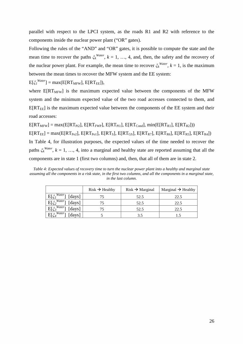
In Table 4, for illustration purposes, the expected values of the time needed to recover the
paths ξkWater, k = 1, …, 4, into a marginal and healthy state are reported assuming that all the
components are in state 1 (first two columns) and, then, that all of them are in state 2.
Table 4: Expected values of recovery time to turn the nuclear power plant into a healthy and marginal state assuming all the components in a risk state, in the first two columns, and all the components in a marginal state,
in the last column.
Risk � Healthy Risk � Marginal Marginal � Healthy
E[ξ1Water] [days] 75 52.5 22.5
E[ξ2Water] [days] 75 52.5 22.5
E[ξ3Water] [days] 75 52.5 22.5
E[ξ4Water] [days] 5 3.5 1.5

27
Figure 12: GTST – DMLD of the case study. MFW: Main Feedwater System; HPCI: High Pressure Coolant Injection System; LPCI: Low Pressure Coolant Injection System; IE: Internal Energy System; DS:
Depressurization System; EW: External Water System; EE: Offsite power system; R: Road access; GS: Generation Station, S: Substation, Po: Pole, Pi: Pipe, CST: Condensate Storage Tank, Cond: Condenser; RP: River Pump, HPP: High Pressure Pump; FWP: Feedwater Pump; LPP: Low Pressure Pump, ADS: Automatic
Depressurization System; DG: Diesel Generator.

28
The states at system-of-systems level depend on the degrees of achievement of the goal
function (Section 2.2.2). Since in the present case study the goal function can be attained by
four different alternative paths (ξ1Water, ξ2
Water, ξ3Water and ξ4
Water), their states identify the state
of the nuclear power plant. We assume that to be in a healthy state at least one path among
ξ1Water, ξ2
Water and ξ3Water, (i.e. water from the main input or the designed internal barriers)
should be in state 3, i.e., healthy, and another path, including also ξ4Water (water from the
external support), should be at least in state 2, i.e., marginal or healthy. To be in a marginal
state, it is necessary that at least one path among ξ1Water, ξ2
Water, ξ3Water and ξ4
Water is at least in
state 2. All the other combinations lead the nuclear power plant plant into a risk state.
Table 5 reports the combination of the states of the possible paths ξkWater, k = 1, …, 4, that
bring the nuclear power plant into a healthy, marginal or risk state.
Table 5: Definition of risk, marginal and healthy states at system-of-systems level with respect to the states of the alternative paths ξk
Water, k = 1, …, 4, that can assure the safety of the nuclear power plant. In the empty space, any state is possible.
ξ1Water ξ2
Water ξ3Water ξ4
Water
Safe
3 3
3 2
3 3
3 2
3 2
3 2
2 3
3 2
3 3
2 3
2 3
3 2
Marginal
2 ~3 ~3 ~3
~3 2 ~3 ~3
~3 ~3 2 ~3
~3 ~3 ~3 2
Risk 1 1 1 1
4.3. Results
The Monte Carlo simulation for Seismic Probabilistic Risk Assessment illustrated in Section
3.3 and Appendix C has been applied to the case study of Section 4.1 for an earthquake with
moment magnitude equal to 5.5 at the epicenter of coordinates (x, y) = (70, 70) (Figure 9,
right). The number of earthquake simulations (NT) is 2000 and the number of recovery time

29
simulations (NRT) for each components configuration that turns the nuclear power plant (NPP)
into a risk or marginal state is 4000.
4.3.1. Safety
Figure 13 shows the comparison of the estimated mean probability that the NPP turns into the
states 1 (risk), 2 (marginal) and 3 (healthy), considering multistate and binary state models for
the components. As expected, the probability to enter into the risk state is similar for both
models (equal to 0.332) and obviously the probability to turn into a marginal state is zero for
the binary state model, since this state is not contemplated in such a model.
Figure 13: Estimate of the probability that the nuclear power plant reaches a risk (1), marginal (2) and healthy (3) state upon occurrence of an earthquake of moment magnitude equal to 5.5, in the case of multistate (grey)
and binary state (black) models.
It can be noticed that the multistate model identifies a criticality in the safety of the NPP,
since it shows that the NPP is mostly in a marginal state (0.605). This means that safety
margins are not satisfied, and the NPP could be exposed to aftershocks. On the contrary, the
binary state model considers these marginal situations as completely safe (healthy), thus
underestimating these situations.
Figure 14 shows the same comparison as in Figure 13, except that, for each of the NT
configurations a sequence of aftershocks is simulated NRT times. These values have been
obtained by adding (and/or subtracting) to the values of Figure 13, the transition probabilities
(Table 6, third column) to enter in (and/or to exit from) the states 1, 2 and 3. These are
obtained by the multiplication of the probabilities that the NPP enters in a certain state after
the earthquake (values of Figure 13) and the conditional transition probabilities (Table 6,
second column) that the NPP degrades into worse states upon the occurrence of aftershocks,
given the state in which it entered after the earthquake.
12
3
0.332
0.605
0.064
0.332
0
0.668
Multistate
Binary

30
Figure 14: Estimate of the probability that the nuclear power plant reaches a risk (1), marginal (2) and healthy (3) state upon occurrence of an earthquake of moment magnitude equal to 5.5 and upon occurrence of
subsequent aftershocks, in the case of multistate (grey) and binary state (black) models.
Table 6: Conditional transition probabilities, given that the NPP entered in a given state after an earthquake (second column), and transition probabilities that the NPP remains in the same state or turns into another
(lower) one after the occurrence of a sequence of aftershocks (third column) for the multistate and binary state models. The transitions considered are reported in the first column.
States transition
(from -> to)
Conditional transition
probability
Transition probability
Multistate
2 -> 1 0.3861 0.2334
2 -> 2 0.6139 0.3711
3 -> 1 0.0597 0.0038
3 -> 2 0.4987 0.0317
3 -> 3 0.4416 0.0280
1 -> 1 1.0000 0.3320
Binary state
3 -> 1 0.0254 0.0170
3 -> 3 0.9746 0.6510
1 -> 1 1.0000 0.3320
From Figure 14, it can be seen that, after a sequence of aftershocks, the probability of the NPP
to turn into a risk state is higher in the case of the multistate model (i.e., 0.569) than in the
case of the binary state model (i.e., 0.349). This is due to the higher probability that the
marginal state of the multistate model turns into a risk state (0.2334, in Table 6) with respect
to the probability that the healthy state of the binary state model turns into a risk state (0.0170,
in Table 6). The first result depends on the definition of marginal state at component and at
system-of-systems levels: i) the components in state 2 are more fragile to withstand
aftershocks (as explained in Section 2.2.1) and ii) in the present simulation, the configurations
of the marginal state of the system of systems after the occurrence of the earthquake are
composed mostly (with probability 0.6940) by only one path ξkWater, k = 1, …, 4, in state 2 and
the others in state 1: thus, they are more exposed to the occurrence of aftershocks than
12
3
0.569
0.403
0.028
0.349
0
0.651
Multistate
Binary

31
configurations composed by all the paths ξkWater, k = 1, …, 4, in state 2 (this situation occurs
with probability equal to 0.007). Instead, the low probability value for the transition from
healthy state to risk state for the binary state model is explained by the fact that, in this case,
there is no distinction among structural and functional state, since they coincide. Therefore,
when the NPP is a healthy state also the components are in a structural and functional healthy
state.
4.3.2. Physical resilience
In the following, the results of evaluation of the physical resilience of the system of systems
are reported. In particular, for the configurations that lead the NPP into a risk state, the
recovery from a state 1 to a state 2 (Figure 15 a), from state 2 to state 3 (Figure 15 b), from
state 1 to state 3, direct and total (Figure 15 c and d, respectively), is analyzed and, for the
configurations that lead the NPP into a marginal state, the recovery from a state 2 to a state 3
(Figure 15 e) is considered.
Figure 15: Illustration of the transitions considered (bold lines) for the analysis of the recovery time with respect to the functional state, zNPP, of the nuclear power plant (NPP).
Figure 16 shows the probability density function (PDF) (on the left) and the respective
cumulative distribution function (CDF) (on the right) of the time necessary to restore the
marginal state of the nuclear power plant from a risk state. As illustrated in the Figure, the
transition into a marginal state of the NPP depends on the transition of one of the alternative
logic paths ξkWater, k = 1, …, 4, into a state 2. The mean of the distribution is 2.6 days.

32
Figure 16: Probability density function (PDF) (on the left) and respective cumulative distribution function (CDF) (on the right) of the time (RT) necessary to restore the marginal state (2) of the nuclear power plant
(NPP) from a risk state (1).
In Figure 17, the frequency of the paths ξkWater, k = 1, …, 4, that perform the transition into the
states 2 or 3 to lead the NPP in a marginal state are reported on the left, and the details of the
frequency of the systems MFW, HPCI, LPCI, DS, IE, EW and EE to be in healthy, marginal
or risk state are illustrated, on the right, with respect to Figure 16.
Figure 17: Left: frequency of the paths ξkWater, k = 1, …, 4, that performing a transition into the states 2 or 3 turn
the nuclear power plant into a marginal state with respect to Figure 16; Right: corresponding frequency of the Main Feedwater (MFW) system, High Pressure Coolant Injection (HPCI) system, Low Pressure Coolant
Injection (LPCI) system, Depressurization System (DS), Internal Energy (IE) system, External Water (EW) system and offsite power (EE) system to be in risk (1), marginal (2) or healthy (3) state.
It can be seen that the transition from the state 1 to the state 2 is mainly due to the path ξkWater,
k = 4, that is formed by the external water system. This system can also turn directly into a
state 3 with probability 0.21 (Figure 17, on the right).
0 10 20 30 40 50 60 70 80 90 100 110 120 130 140 1500
0.05
0.1
0.15
0.2
0.25
0.3P
roba
bilit
y D
ensi
ty F
unct
ion
0 10 20 30 40 50 60 70 80 90 100 110 120 130 140 1500
0.1
0.2
0.3
0.4
0.5
0.6
0.7
0.8
0.9
1
Cum
ulat
ive
Dis
trib
utio
n F
unct
ion
0.0
0.2
0.4
0.6
0.8
1.0
0.139
0.034 0.034
0.603
0.0160.002 0.002
0.2112
3 0.0
0.2
0.4
0.6
0.8
1.0 0.840.96
0.96
0.08 0.180.01
0.140.03
0.03
0.60
10.92
0.21
0.99
1
2
3
ξ1Water ξ2
Water ξ3
Water ξ4Water
)21()1(
→NPPRT [days] )21(
)1(→
NPPRT [days]
33
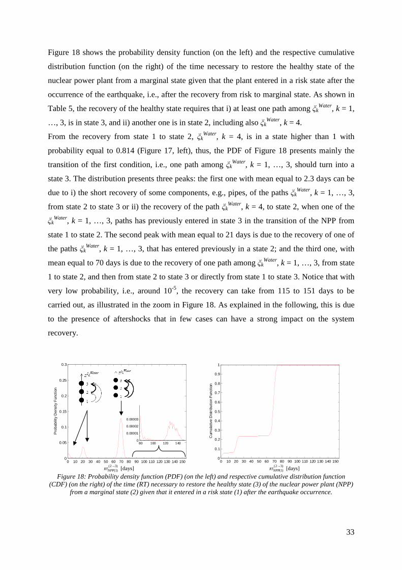
Figure 18 shows the probability density function (on the left) and the respective cumulative
distribution function (on the right) of the time necessary to restore the healthy state of the
nuclear power plant from a marginal state given that the plant entered in a risk state after the
occurrence of the earthquake, i.e., after the recovery from risk to marginal state. As shown in
Table 5, the recovery of the healthy state requires that i) at least one path among ξkWater, k = 1,
…, 3, is in state 3, and ii) another one is in state 2, including also ξkWater, k = 4.
From the recovery from state 1 to state 2, ξkWater, k = 4, is in a state higher than 1 with
probability equal to 0.814 (Figure 17, left), thus, the PDF of Figure 18 presents mainly the
transition of the first condition, i.e., one path among ξkWater, k = 1, …, 3, should turn into a
state 3. The distribution presents three peaks: the first one with mean equal to 2.3 days can be
due to i) the short recovery of some components, e.g., pipes, of the paths ξkWater, k = 1, …, 3,
from state 2 to state 3 or ii) the recovery of the path ξkWater, k = 4, to state 2, when one of the
ξkWater, k = 1, …, 3, paths has previously entered in state 3 in the transition of the NPP from
state 1 to state 2. The second peak with mean equal to 21 days is due to the recovery of one of
the paths ξkWater, k = 1, …, 3, that has entered previously in a state 2; and the third one, with
mean equal to 70 days is due to the recovery of one path among ξkWater, k = 1, …, 3, from state
1 to state 2, and then from state 2 to state 3 or directly from state 1 to state 3. Notice that with
very low probability, i.e., around 10-5, the recovery can take from 115 to 151 days to be
carried out, as illustrated in the zoom in Figure 18. As explained in the following, this is due
to the presence of aftershocks that in few cases can have a strong impact on the system
recovery.
Figure 18: Probability density function (PDF) (on the left) and respective cumulative distribution function (CDF) (on the right) of the time (RT) necessary to restore the healthy state (3) of the nuclear power plant (NPP)
from a marginal state (2) given that it entered in a risk state (1) after the earthquake occurrence.
0 10 20 30 40 50 60 70 80 90 100 110 120 130 140 1500
0.05
0.1
0.15
0.2
0.25
0.3
Pro
babi
lity
Den
sity
Fun
ctio
n
0 10 20 30 40 50 60 70 80 90 100 110 120 130 140 1500
0.1
0.2
0.3
0.4
0.5
0.6
0.7
0.8
0.9
1
Cum
ula
tive
Dis
trib
utio
n F
unct
ion
)32()1(
→NPPRT [days] )32(
)1(→
NPPRT [days]
80 100 120 1400
0.00001
0.00002
0.00003
34
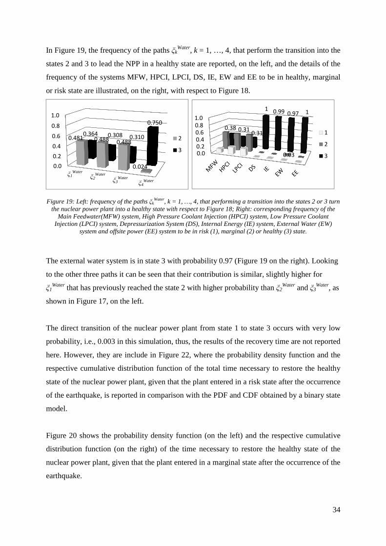
In Figure 19, the frequency of the paths ξkWater, k = 1, …, 4, that perform the transition into the
states 2 and 3 to lead the NPP in a healthy state are reported, on the left, and the details of the
frequency of the systems MFW, HPCI, LPCI, DS, IE, EW and EE to be in healthy, marginal
or risk state are illustrated, on the right, with respect to Figure 18.
Figure 19: Left: frequency of the paths ξkWater, k = 1, …, 4, that performing a transition into the states 2 or 3 turn
the nuclear power plant into a healthy state with respect to Figure 18; Right: corresponding frequency of the Main Feedwater(MFW) system, High Pressure Coolant Injection (HPCI) system, Low Pressure Coolant
Injection (LPCI) system, Depressurization System (DS), Internal Energy (IE) system, External Water (EW) system and offsite power (EE) system to be in risk (1), marginal (2) or healthy (3) state.
The external water system is in state 3 with probability 0.97 (Figure 19 on the right). Looking
to the other three paths it can be seen that their contribution is similar, slightly higher for
ξ1Water that has previously reached the state 2 with higher probability than ξ2
Water and ξ3Water, as
shown in Figure 17, on the left.
The direct transition of the nuclear power plant from state 1 to state 3 occurs with very low
probability, i.e., 0.003 in this simulation, thus, the results of the recovery time are not reported
here. However, they are include in Figure 22, where the probability density function and the
respective cumulative distribution function of the total time necessary to restore the healthy
state of the nuclear power plant, given that the plant entered in a risk state after the occurrence
of the earthquake, is reported in comparison with the PDF and CDF obtained by a binary state
model.
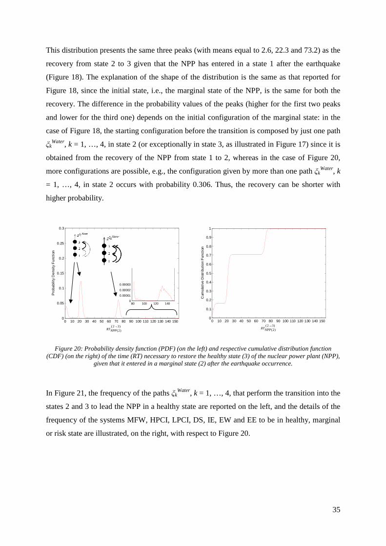
Figure 20 shows the probability density function (on the left) and the respective cumulative
distribution function (on the right) of the time necessary to restore the healthy state of the
nuclear power plant, given that the plant entered in a marginal state after the occurrence of the
earthquake.
0.0
0.2
0.4
0.6
0.8
1.0
0.481 0.4880.488
0.024
0.364 0.308 0.310
0.750
2
30.00.2
0.4
0.6
0.8
1.0
0.03
0.38 0.310.31
1 0.99 0.97 1
1
2
3
ξ1Water ξ2
Water ξ3
Water ξ4Water
35
This distribution presents the same three peaks (with means equal to 2.6, 22.3 and 73.2) as the
recovery from state 2 to 3 given that the NPP has entered in a state 1 after the earthquake
(Figure 18). The explanation of the shape of the distribution is the same as that reported for
Figure 18, since the initial state, i.e., the marginal state of the NPP, is the same for both the
recovery. The difference in the probability values of the peaks (higher for the first two peaks
and lower for the third one) depends on the initial configuration of the marginal state: in the
case of Figure 18, the starting configuration before the transition is composed by just one path
ξkWater, k = 1, …, 4, in state 2 (or exceptionally in state 3, as illustrated in Figure 17) since it is
obtained from the recovery of the NPP from state 1 to 2, whereas in the case of Figure 20,
more configurations are possible, e.g., the configuration given by more than one path ξkWater, k
= 1, …, 4, in state 2 occurs with probability 0.306. Thus, the recovery can be shorter with
higher probability.
Figure 20: Probability density function (PDF) (on the left) and respective cumulative distribution function (CDF) (on the right) of the time (RT) necessary to restore the healthy state (3) of the nuclear power plant (NPP),
given that it entered in a marginal state (2) after the earthquake occurrence.
In Figure 21, the frequency of the paths ξkWater, k = 1, …, 4, that perform the transition into the
states 2 and 3 to lead the NPP in a healthy state are reported on the left, and the details of the
frequency of the systems MFW, HPCI, LPCI, DS, IE, EW and EE to be in healthy, marginal
or risk state are illustrated, on the right, with respect to Figure 20.
0 10 20 30 40 50 60 70 80 90 100 110 120 130 140 1500
0.05
0.1
0.15
0.2
0.25
0.3
Pro
babi
lity
Den
sity
Fun
ctio
n
0 10 20 30 40 50 60 70 80 90 100 110 120 130 140 1500
0.1
0.2
0.3
0.4
0.5
0.6
0.7
0.8
0.9
1
Cum
ula
tive
Dis
trib
utio
n F
unct
ion
)32()2(
→NPPRT
)32()2(
→NPPRT
80 100 120 1400
0.00001
0.00002
0.00003
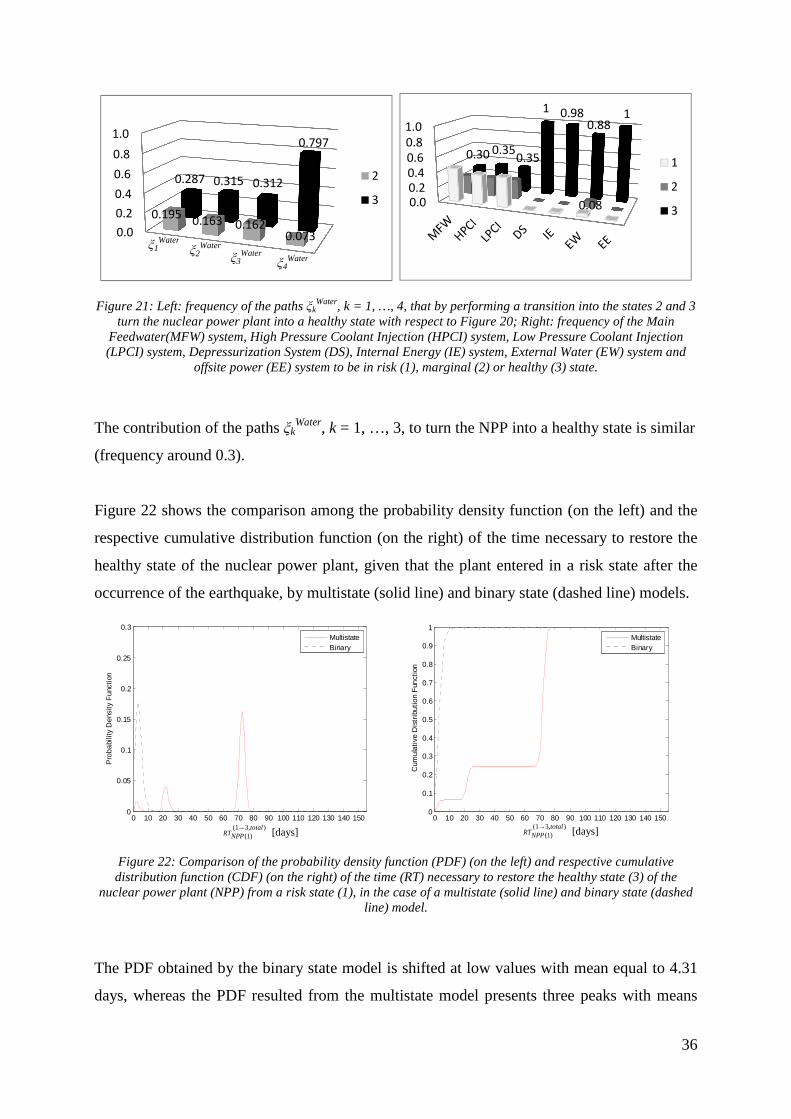
36
Figure 21: Left: frequency of the paths ξkWater, k = 1, …, 4, that by performing a transition into the states 2 and 3
turn the nuclear power plant into a healthy state with respect to Figure 20; Right: frequency of the Main Feedwater(MFW) system, High Pressure Coolant Injection (HPCI) system, Low Pressure Coolant Injection (LPCI) system, Depressurization System (DS), Internal Energy (IE) system, External Water (EW) system and
offsite power (EE) system to be in risk (1), marginal (2) or healthy (3) state.
The contribution of the paths ξkWater, k = 1, …, 3, to turn the NPP into a healthy state is similar
(frequency around 0.3).
Figure 22 shows the comparison among the probability density function (on the left) and the
respective cumulative distribution function (on the right) of the time necessary to restore the
healthy state of the nuclear power plant, given that the plant entered in a risk state after the
occurrence of the earthquake, by multistate (solid line) and binary state (dashed line) models.
Figure 22: Comparison of the probability density function (PDF) (on the left) and respective cumulative distribution function (CDF) (on the right) of the time (RT) necessary to restore the healthy state (3) of the
nuclear power plant (NPP) from a risk state (1), in the case of a multistate (solid line) and binary state (dashed line) model.
The PDF obtained by the binary state model is shifted at low values with mean equal to 4.31
days, whereas the PDF resulted from the multistate model presents three peaks with means
0.0
0.2
0.4
0.6
0.8
1.0
0.1950.163 0.162
0.073
0.287 0.315 0.312
0.797
2
3 0.0
0.2
0.4
0.6
0.8
1.0
0.08
0.30 0.350.35
1 0.980.88
1
1
2
3
0 10 20 30 40 50 60 70 80 90 100 110 120 130 140 1500
0.05
0.1
0.15
0.2
0.25
0.3
Recovery time 1 -> 3 - total [days]
Pro
babi
lity
Den
sity
Fun
ctio
n
MultistateBinary
0 10 20 30 40 50 60 70 80 90 100 110 120 130 140 1500
0.1
0.2
0.3
0.4
0.5
0.6
0.7
0.8
0.9
1
Recovery time 1 -> 3 - tot [days]
Cum
ula
tive
Dis
trib
utio
n F
unct
ion
MultistateBinary
ξ1Water ξ2
Water ξ3
Water ξ4Water
),31()1(total
NPPRT→ [days]
),31()1(total
NPPRT→ [days]
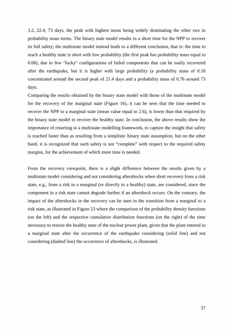
37
3.2, 22.4, 73 days, the peak with highest mean being widely dominating the other two in
probability mass terms. The binary state model results in a short time for the NPP to recover
its full safety; the multistate model instead leads to a different conclusion, that is: the time to
reach a healthy state is short with low probability (the first peak has probability mass equal to
0.06), due to few "lucky" configurations of failed components that can be easily recovered
after the earthquake, but it is higher with large probability (a probability mass of 0.18
concentrated around the second peak of 21.4 days and a probability mass of 0.76 around 73
days.
Comparing the results obtained by the binary state model with those of the multistate model
for the recovery of the marginal state (Figure 16), it can be seen that the time needed to
recover the NPP to a marginal state (mean value equal to 2.6), is lower than that required by
the binary state model to recover the healthy state. In conclusion, the above results show the
importance of resorting to a multistate modelling framework, to capture the insight that safety
is reached faster than as resulting from a simplistic binary state assumption, but on the other
hand, it is recognized that such safety is not “complete” with respect to the required safety
margins, for the achievement of which more time is needed.
From the recovery viewpoint, there is a slight difference between the results given by a
multistate model considering and not considering aftershocks when short recovery from a risk
state, e.g., from a risk to a marginal (or directly to a healthy) state, are considered, since the
component in a risk state cannot degrade further if an aftershock occurs. On the contrary, the
impact of the aftershocks in the recovery can be seen in the transition from a marginal to a
risk state, as illustrated in Figure 23 where the comparison of the probability density functions
(on the left) and the respective cumulative distribution functions (on the right) of the time
necessary to restore the healthy state of the nuclear power plant, given that the plant entered in
a marginal state after the occurrence of the earthquake considering (solid line) and not
considering (dashed line) the occurrence of aftershocks, is illustrated.

38
Figure 23: Comparison of the probability density functions (PDFs) (on the left) and respective cumulative distribution functions (CDFs) (on the right) of the time (RT) necessary to restore the healthy state (3) of the nuclear power plant (NPP), given that it entered in a marginal state (2) after the earthquake occurrence, considering (solid line) and not considering (dashed line) the occurrence of aftershocks.
The two probability density functions show the same peaks with mean around 2.5, 22.2, 73.2
days, but in the case with aftershocks the probability values are lower for the first two peaks
and higher for the third one than in the case without aftershocks. Thus, in the case with
aftershocks, the probability that the recovery needs more time is higher; in addition, there is a
small probability, i.e., around 10-6, that the recovery is carried out in more than 120 days, as
illustrated in the zoom of Figure 23.
5. CONCLUSIONS
We have significantly extended a system-of-systems framework previously proposed by the
authors for the analysis of the risk of a critical plant (e.g., a nuclear power plant) from natural
external events (e.g., earthquakes).
We have explicitly modelled the different parts of the system-of-systems into i) main inputs,
i.e., the infrastructure systems devoted to provide the main supply for the safety of the nuclear
power plant, ii) internal barriers, i.e., the internal emergency devices designed to
automatically activate in emergency conditions, iii) external supports, i.e., the redundant
infrastructure systems that can replace the main inputs and the internal barriers when they do
not function, iv) the recovery supporting elements, i.e., the infrastructure systems that can be a
support in the actions to keep or restore the safety of the plant.
We have adopted a multistate model distinguishing structural damage and functional
performance of the individual components, that reflects into a multistate model of the system
0 10 20 30 40 50 60 70 80 90 100 110 120 130 140 1500
0.05
0.1
0.15
0.2
0.25
0.3
Recovery time 2 -> 3 (2) [days]
Pro
babi
lity
Den
sity
Fun
ctio
n
AftershocksNo aftershocks
0 10 20 30 40 50 60 70 80 90 100 110 120 130 140 1500
0.1
0.2
0.3
0.4
0.5
0.6
0.7
0.8
0.9
1
Recovery time 2 -> 3 (2) [days]
Cum
ula
tive
Dis
trib
utio
n F
unct
ion
AftershocksNo aftershocks
80 100 120 1400
0.00001
0.00002
0.00003
)32()2(
→NPPRT
)32()2(
→NPPRT

39
of systems based on different degrees of safety (risk, marginal and healthy) of the nuclear
power plant.
We have represented the system of systems with a Goal Tree Success Tree – Dynamic Master
Logic Diagram (GTST-DMLD) and we have used Monte Carlo simulation for the
probabilistic evaluation of the safety of the nuclear power plant and its physical resilience,
measured in terms of the time needed to restore the safety. In addition, we have included the
impacts of aftershocks.
In particular, by exemplification of a case study concerning the seismic risk of a nuclear
power plant, the following analyses have been carried out:
a. a comparison between the probabilities that the nuclear power plant enters in risk,
marginal and healthy states calculated by multistate and binary state models: as
expected, the probability to enter in a risk state is the same for both models, whereas
the probability to be in a healthy state is lower for the multistate model that identifies
(marginal) configurations of the system of systems that present criticalities because
not satisfying safety margins;
b. a comparison of the previous probabilities (a.) considering also sequences of
aftershocks that could further degrade the safety of the nuclear power plant. The
multistate models evidences a higher probability that the nuclear power plant enters
into a risk state (+ 0.2372) than the binary state model (+ 0.0170). Thus, it can capture
the impact of the aftershocks that are almost neglected by the binary state model since
the structural healthy state of the components is characterized by fragilities that are not
much sensitive to small ground motion levels produced by aftershocks. Actually, the
increased probability of the risk state is mainly (0.2334) due to the degradation of the
marginal state that is more exposed to aftershocks than the healthy state;
c. a comparison of the probability density function (PDF) and the respective cumulative
distribution function (CDF) of the time necessary to restore the healthy state of the
nuclear power plant, given that the plant has entered in a marginal and risk state, and
the recovery time of the marginal state given that the plant has entered in risk state,
with the i) binary state model and ii) multistate model without considering the
occurrence of the aftershocks:
i) From the first comparison, it can be seen that the binary state model is less
conservative than the multistate model in that it identifies a mean time to
recover the healthy state lower than the one identified by the multistate model,

40
but higher than the one needed to recover a marginal state. On the contrary, the
multistate model is capable of capturing the fact that a faster recovery to reach
a safe condition is possible, but this condition is marginal with respect to the
safety margins and a longer time is needed to arrive at a completely safe state,
including the safety margins.
ii) From the second comparison, important differences cannot be seen in the
recovery time distribution for fast recovery from risk states, e.g., from risk to
marginal state, since, in this work, a component in risk state cannot further
degrade into a worse state. A further development of the model will be done in
the future to take into account the disturbance of the aftershocks for the
components in risk state. On the contrary, the impact of aftershocks is evident
in the recovery from a marginal state to healthy state since the components in
state 2 can degrade to state 1 more than once during the total recovery. As a
consequence, the time needed for the restoration of the healthy state increases
considering the occurrence of aftershocks.
The results obtained, albeit performed on a simplified case study and under limiting
assumptions, highlight that the multistate model is relevant to identify marginal conditions of
safety of the critical plant that may turn into a risk state. This can be relevant for the decision
making related to safety-critical issues when external events occur: a marginal condition may
degrade to a risky one but this would not happen (or it would happen with very small
probability, e.g, 0.0038 in the present case study) for a complete safe state that can mainly
degrade to a marginal state. On the contrary, the binary state model does not allow these
considerations since it does not distinguish different safety levels; in this case, a complete safe
state can directly change into a risk state. However, this is not evident in the simulation: the
healthy state turns into a risk state with probability 0.0170 (Section 4.3.1), as explained in the
point b. above. Thus, the multistate model allows identifying criticalities that are hidden in a
binary model and that can lead to an underestimation of the risk. The multistate model is more
conservative than the binary state one; this can be seen also from the results related to the
system resilience characteristics, where the time necessary to restore the complete safety is
longer than that needed with a binary state model for most of the cases. However, as
explained before, the complete safety of the binary state model hides criticalities and it can be
affected by aftershocks. The multistate model, instead, shows that restoration of the marginal
safety can occur in a shorter time; the faster recovery is associated with the awareness that

41
safety margins are not satisfied. These findings can help to improve the structural/functional
responses of the critical elements of the alternative logic paths, for improving the global
resilience of the system of systems so as to increase the safety of the critical plant. The
multistate model is a valid support for achieving these goals, provided that the definition of
the structural and functional limit states is carefully addressed.
Future work will be devoted to apply the framework of analysis presented to a critical
networked infrastructure and to consider advanced simulation techniques in order to render
more efficient the computation.
REFERENCES
[1] Manyena SB. The concept of resilience revisited. Disasters. 2006; 30:434-450.
[2] Cimellaro GP, Reinhorn AM, Bruneau M. Framework for analytical quantification of
disaster resilience. Engineering Structures. 2010; 32: 3639-3649.
[3] Zio E, Ferrario E. A framework for the system-of-systems analysis of the risk for a
safety- critical plant exposed to external events. Reliability Engineering and System
Safety. 2013; 114: 114-225.
[4] Li Y, van de Lindt JW. Loss-based formulation for multiple hazards with application to
residential buildings. Engineering Structures. 2012; 38: 123-133.
[5] Selva J, Kakderi K, Alexoudi M, Pitilakis K. Seismic performance of a system of
interdependent lifeline and infrastructure components. 8th International Conference on
urban Earthquake Engineering, Tokio Institute of Technology, Japan. 2011.
[6] Billinton R, Karki R. Application of Monte Carlo simulation to generating system well-
being analysis. Power Systems, IEEE Transactions on. 1999; 14(3):1172-1177.
[7] Hu YS, Modarres M. Evaluating system behavior through Dynamic Master Logic
Diagram (DMLD) modeling. Reliability Engineering and System Safety. 1999; 64:241-
269.
[8] Kalos MH, Whitlock PA. Monte Carlo methods. Vol. 1, Basics. New York: Wiley;
1986. 186 p.
[9] Zio E. Computational methods for reliability and risk analysis. Series on Quality,
Reliability and Engineering Statistics, Vol 14. Singapore: World Scientific Publishing
Co. Pte. Ltd.; 2009. Chapter 2, Monte Carlo simulations for reliability and availability
analysis; p. 59-69.
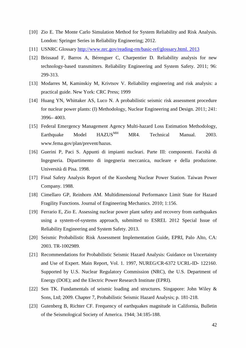
42
[10] Zio E. The Monte Carlo Simulation Method for System Reliability and Risk Analysis.
London: Springer Series in Reliability Engineering; 2012.
[11] USNRC Glossary http://www.nrc.gov/reading-rm/basic-ref/glossary.html. 2013
[12] Brissaud F, Barros A, Bérenguer C, Charpentier D. Reliability analysis for new
technology-based transmitters. Reliability Engineering and System Safety. 2011; 96:
299-313.
[13] Modarres M, Kaminskiy M, Krivtsov V. Reliability engineering and risk analysis: a
practical guide. New York: CRC Press; 1999
[14] Huang YN, Whittaker AS, Luco N. A probabilistic seismic risk assessment procedure
for nuclear power plants: (I) Methodology, Nuclear Engineering and Design. 2011; 241:
3996– 4003.
[15] Federal Emergency Management Agency Multi-hazard Loss Estimation Methodology,
Earthquake Model HAZUSMH MR4. Technical Manual. 2003.
www.fema.gov/plan/prevent/hazus.
[16] Guerini P, Paci S. Appunti di impianti nucleari. Parte III: componenti. Facoltà di
Ingegneria. Dipartimento di ingegneria meccanica, nucleare e della produzione.
Università di Pisa. 1998.
[17] Final Safety Analysis Report of the Kuosheng Nuclear Power Station. Taiwan Power
Company. 1988.
[18] Cimellaro GP, Reinhorn AM. Multidimensional Performance Limit State for Hazard
Fragility Functions. Journal of Engineering Mechanics. 2010; 1:156.
[19] Ferrario E, Zio E. Assessing nuclear power plant safety and recovery from earthquakes
using a system-of-systems approach, submitted to ESREL 2012 Special Issue of
Reliability Engineering and System Safety. 2013.
[20] Seismic Probabilistic Risk Assessment Implementation Guide, EPRI, Palo Alto, CA:
2003. TR-1002989.
[21] Recommendations for Probabilistic Seismic Hazard Analysis: Guidance on Uncertainty
and Use of Expert. Main Report, Vol. 1. 1997, NUREG/CR-6372 UCRL-ID- 122160.
Supported by U.S. Nuclear Regulatory Commission (NRC), the U.S. Department of
Energy (DOE); and the Electric Power Research Institute (EPRI).
[22] Sen TK. Fundamentals of seismic loading and structures. Singapore: John Wiley &
Sons, Ltd; 2009. Chapter 7, Probabilistic Seismic Hazard Analysis; p. 181-218.
[23] Gutenberg B, Richter CF. Frequency of earthquakes magnitude in California, Bulletin
of the Seismological Society of America. 1944; 34:185-188.
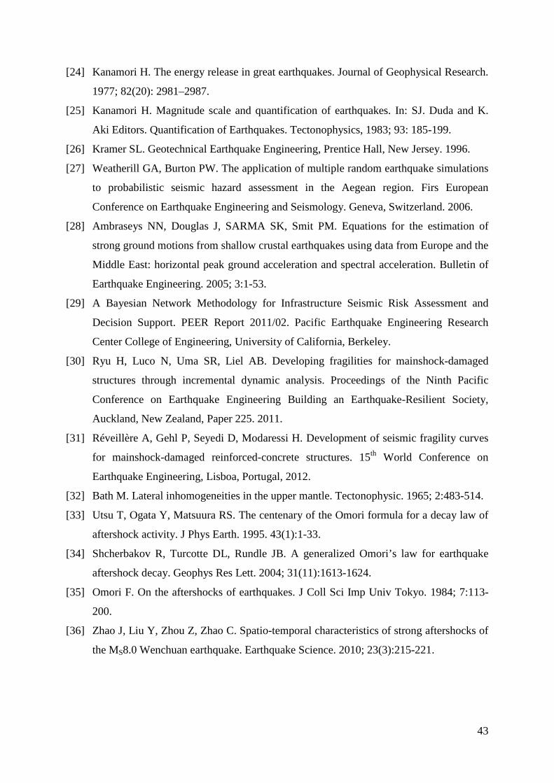
43
[24] Kanamori H. The energy release in great earthquakes. Journal of Geophysical Research.
1977; 82(20): 2981–2987.
[25] Kanamori H. Magnitude scale and quantification of earthquakes. In: SJ. Duda and K.
Aki Editors. Quantification of Earthquakes. Tectonophysics, 1983; 93: 185-199.
[26] Kramer SL. Geotechnical Earthquake Engineering, Prentice Hall, New Jersey. 1996.
[27] Weatherill GA, Burton PW. The application of multiple random earthquake simulations
to probabilistic seismic hazard assessment in the Aegean region. Firs European
Conference on Earthquake Engineering and Seismology. Geneva, Switzerland. 2006.
[28] Ambraseys NN, Douglas J, SARMA SK, Smit PM. Equations for the estimation of
strong ground motions from shallow crustal earthquakes using data from Europe and the
Middle East: horizontal peak ground acceleration and spectral acceleration. Bulletin of
Earthquake Engineering. 2005; 3:1-53.
[29] A Bayesian Network Methodology for Infrastructure Seismic Risk Assessment and
Decision Support. PEER Report 2011/02. Pacific Earthquake Engineering Research
Center College of Engineering, University of California, Berkeley.
[30] Ryu H, Luco N, Uma SR, Liel AB. Developing fragilities for mainshock-damaged
structures through incremental dynamic analysis. Proceedings of the Ninth Pacific
Conference on Earthquake Engineering Building an Earthquake-Resilient Society,
Auckland, New Zealand, Paper 225. 2011.
[31] Réveillère A, Gehl P, Seyedi D, Modaressi H. Development of seismic fragility curves
for mainshock-damaged reinforced-concrete structures. 15th World Conference on
Earthquake Engineering, Lisboa, Portugal, 2012.
[32] Bath M. Lateral inhomogeneities in the upper mantle. Tectonophysic. 1965; 2:483-514.
[33] Utsu T, Ogata Y, Matsuura RS. The centenary of the Omori formula for a decay law of
aftershock activity. J Phys Earth. 1995. 43(1):1-33.
[34] Shcherbakov R, Turcotte DL, Rundle JB. A generalized Omori’s law for earthquake
aftershock decay. Geophys Res Lett. 2004; 31(11):1613-1624.
[35] Omori F. On the aftershocks of earthquakes. J Coll Sci Imp Univ Tokyo. 1984; 7:113-
200.
[36] Zhao J, Liu Y, Zhou Z, Zhao C. Spatio-temporal characteristics of strong aftershocks of
the MS8.0 Wenchuan earthquake. Earthquake Science. 2010; 23(3):215-221.

44
APPENDIX A. Qualities, parts and GTST-DMLD within a system-of-
systems framework: an example
For illustration purpose, let us consider the main function F* of a critical plant H, i.e., the
critical element E, achieved through the success of two principal functions, F1 and F2, where
the former is in turn obtained by the combination of functions F1,1 and F1,2. In addition, we
consider an auxiliary function F3 that is not needed directly for achieving F* , but it serves the
function F2. In the hierarchy, the function F3 is represented in a parallel branch connected to
F* by a dashed line (Figure A.1).
Figure A.1: Hierarchy of the qualities of the example proposed.
Figure A.2 represents the graph of the components of this example with respect to the safety
levels of Figure 2. The links show the relationship among the components; they are directed
from an element to another dependent on it. The safety of a critical element � (star) is assured
by A = 8 systems divided into nMI = 1 system of main inputs, S(1), nIB = 3 internal barriers,
S(2), S(3) and S(4), nES = 2 external supports, S(5) and S(6), nRS = 2 recovery supporting elements,
S(7) and S(8), represented in dashed oval shape. The components included in these systems are
represented in solid oval shape. For example, the system S(1) is formed by 3 components (S1(1),
S2(1), S3
(1)), the system S(2) is composed by 1 component, S1(2), and so on. Notice that there are
some components that are directly connected to E, e.g., S3(1) and S1
(2), and others that are
connected to the components of other systems, e.g., S1(3) is connected to S1
(2). The first type of
components belongs to principal systems, whereas the latter one to the auxiliary systems,
except for the recovery supporting elements that are considered apart from these systems for
their role of recovery, as explained in Section 2.1. Each system S(a), a = 1, …, 8, can be
represented in the form of a hierarchy as illustrated in Figure A.3.

45
Figure A.2: Graph of the physical components for the example proposed.
Figure A.3: Hierarchy of the parts of the example proposed; nMI, nIB, nES, nRS refer to the number of main inputs, internal barriers, external supports and recovery supporting elements, respectively.
In Figure A.4, the GTST-DMLD of the example above is reported. The goal tree is the
hierarchy of Figure A.1 and the success tree is composed by the hierarchies of Figure A.3.
The dot- and square- dependencies detail the connections of the graph of Figure A.2 and
connect the physical elements to the functions.

46
Figure A.4: GTST – DMLD of the example considered.
APPENDIX B. Seismic Probabilistic Risk Assessment
Since the exemplification of the modelling framework is done with reference to a nuclear
power plant as critical plant and earthquakes as the external events, in Appendix B.1 some
basic information on the procedure for Seismic Probabilistic Risk Assessment (SPRA) of a
nuclear power plant is given; aftershocks are also considered (Appendix B.2).
B.1 Seismic risk
The risk on a system deriving from an earthquake (hereafter referred to as the main shock) is
evaluated by a procedure of Seismic Probabilistic Risk Assessment (SPRA) that consists of
three parts: i) Seismic Hazard Analysis, ii) Seismic Fragility Evaluation and iii) System
Analysis [20].
47
The first part is aimed at computing the probabilities of occurrence of different levels of
earthquake ground motion at a site of interest. It is traditionally developed as a Probabilistic
Seismic Hazard Analysis (PSHA) consisting of four procedural steps [20], [21], [22]:
1) Identification and characterization of the earthquake source;
2) Definition of the earthquake recurrence relationship, i.e., the annual frequency of
occurrence of a given magnitude event for each source, typically described by the
Gutenberg-Richter law [23]:
log(netq) = a – bmetq (B.1)
where netq is the number of earthquakes with magnitude1 greater than metq, and a and b
are parameters obtained by data regression analysis [20], [21], [22]. This relation
implies a double truncated distribution for the magnitude [26], [27]:
)(
)(
minmax
min
1
1)(
etqetq
etqetq
mm
mmetq
Me
emF
−−
−−
−
−=β
β (B.2)
where β represents the relative frequency of smaller to larger events, and etqmmax and
etqmmin are the upper and lower bounds of the magnitude, respectively, that avoid the
high values which are unrealistic and the low values that are negligible.
3) Formulation of the ground motion attenuation relationship that identifies the ground
motion value at the site of interest, e.g., the peak ground acceleration, given the
source-to-site distance and the magnitude. The higher the distance from the source, the
lower is the ground motion value. The following relationship described by [28] has
been adopted in this paper:
010987625
210432110 log*)('log FCFCFCSCSCCrmCCmCCz TNAS
etqetq +++++++++= (B.3)
where metq is the earthquake magnitude, r is the source-to-site distance, SS and SA
represent the types of soil (soft, stiff or rock, when both variables are set to zero) and
FN, FT and FO describe the faulting mechanism (normal, thrust or odd). Equation B.3
has been derived by weighted regression analysis on a set of strong-motion records
collected in Europe and in Middle Est [28].
4) Computation of the exceedance probability of ground motion in any time interval by
analytical integration for each magnitude, distance and ground motion value.
1 The magnitude scale typically used is the moment magnitude defined by [24]. For medium size earthquakes it
is similar to the Richter values [25].
48
The second part of the SPRA identifies the seismic capacity of a component in terms of its
conditional probability of failure f’ for any given ground motion level z’ [20]:
( )
Φ+Φ=−
r
um QAzf
ββ )(/'log
'1
(B.4)
where Q is the subjective probability of not exceeding a fragility f’ , Am is the median
acceleration capacity, βr and βu are the logarithmic standard deviation due to randomness and
to uncertainty in the median capacity, respectively. Considering different damage states of a
component, “failure” means generically “degree of damage”: thus, the fragility is the
conditional probability of exceeding a level of damage for any given ground motion level
[29]. The damage states are therefore identified by the fragility curves. A fragility evaluation
is carried out to provide the parameter values (Am, βr and βu) for the fragility model. This
evaluation is performed for critical failure modes by considering safety margins inherent in
capacity predictions, response analysis and equipment qualification [20]. Recent studies [30],
[31] have been devoted to identifying methodologies for developing “aftershocks fragilities”,
i.e., fragility curves for main shock-damaged structures that are initially in a given damage
state due to the occurrence of an earthquake. Since the estimation of the fragility parameters is
not the objective of the present work, in our evaluation we have assumed arbitrarily the
parameter values to determine the damage states due to main shocks and aftershocks (see
Section 4.1.1).
In the third part, the outputs of the hazard and fragility analyses are integrated to evaluate the
impact of an external event to the system of interest [20]. In this work, we adopt a Goal Tree
Success Tree – Dynamic Master Logic Diagram (GTST-DMLD) representation for the
analysis of the impact on the system and Monte Carlo simulation for the quantitative
evaluation. In extreme synthesis, Monte Carlo simulation is used for determining the state of
each component of the system as a result of the impact of the external event on the component
given its fragility in terms of its probability of exceeding different damage states for a given
ground motion level. Then, the GTST-DMLD accounts for the dependencies among all the
components and their states for determining the state of the entire system due to the impact of
the external event. This part is described in detail in Section 3 and Appendix C.

49
B.2 Aftershocks
Aftershocks, small earthquakes that occur naturally after the main shock, can further degrade
the conditions of a component or a system. In this work, we compute their impacts on the
system of interest by the same SPRA procedure explained above for the earthquake
(Appendix B.1).
According to Bath’s law [32], the difference, ∆, between the magnitude of an earthquake,
metq, and of its largest aftershock, afmmax , is a constant, independent on the earthquake
magnitude, and typically approximated to 1.2:
2.1max =−= afetqmm� (B.5)
As for the earthquake, the recurrence relationship of aftershocks is described by the
Gutenberg-Richter law (eq. B.1) and their magnitude, maf, is still represented by the double
truncated distribution of eq. B.2, computing the maximum magnitude, afmmax , from eq. B.5 and
defining a minimum magnitude, afmmin , of interest.
The temporal decay activity of aftershocks follows the modified Omori’s law [33], [34]:
ptc
Wt
)()(
+=λ (B.6)
where λ(t) is the occurrence rate of aftershocks with magnitude greater than the minimum
magnitude of aftershocks considered, afmmin , t is the time passed from the earthquake and p, c
and W are parameters which depend on the geophysics of the environment. Assuming p = 1,
as in the original formulation of the Omori’s law [35], and fixing the value of the parameter c,
e.g., c = 0.05 [36], it is possible to identify the parameter W comparing the integral of eq. B.6
in a time window [0, T*] (e.g., [0, 365] days [36]) with the maximum number of aftershocks,
afnmax , that can occur in one year [36]:
∫ =+
*
0 max)(
T afp
ndttc
W , (B.7)
where afmbaafn min
max*
10−= from the Gutenberg-Richter law (eq. B.1).
Once that all the parameters of the occurrence rate λ(t) are determined, the number of
aftershocks in the intervals of time [0 Ti], Ti = 1, 2, …, T*, can be computed by solving the
integral of eq. B.7. Normalizing these values with respect to the maximum number of
aftershocks, afnmax , we can obtain the cumulative distribution function (CDF) of the occurrence
time of aftershocks.

50
In this work we have considered the occurrence of an earthquake of magnitude, metq, equal to
5.5 on the moment magnitude scale, followed by a sequence of aftershocks whose minimum
moment magnitude value, afmmin , is 3 (assumed) and the maximum, af
mmax , is 4.3 (computed by
eq. B.5). We have fixed the parameter b of the Gutenberg-Richter law to 1, since it can vary
in the range 1 ± 0.3 [26], and we have computed the parameter a of the same law by assuming
naf = 1 with respect to the magnitude of the largest aftershock, afmmax , i.e., by assuming that an
aftershock that has a magnitude equal to that of the largest aftershock can occur once in a
year. Then, given the parameters a (a = 4.3) and b we have obtained afnmax = 20 from the
Gutenberg-Richter law, considering the magnitude afmmin . Assuming the parameters p = 1 [35]
and c = 0.05 [36], we have determined the value of W (W = 2.25) from eq. B.7 in a time
window equal to [0, 365] days. The CDF obtained is illustrated in Figure B.1.
Figure B.1: Cumulative distribution function (CDF) of the occurrence time of aftershocks.
APPENDIX C. Monte Carlo simulation for Seismic Probabilistic Risk
Assessment within a system-of-systems framework: operative steps
The simulation procedure consists of the following operative steps:
1. choose a value of earthquake magnitude and epicenter coordinates with respect to
which the analysis is performed;
2. compute by eq. B.3 the ground acceleration value at each of the η, η = 1, …, L,
components in the last levels of the physical hierarchies of the systems S(a), a = 1, …,
A; L is the total number of components of the system of systems;
0 50 100 150 200 250 300 3500
0.1
0.2
0.3
0.4
0.5
0.6
0.7
0.8
0.9
1
time [days]
CD
F

51
3. compute the fragilities, {f}, for all the components of the system of systems by eq.
B.4; {f} is a matrix of 2 x L values (two for each component), representing the
conditional probability of exceeding a marginal (f1,η, η = 1, …, L) and risk (f2,η, η = 1,
…, L) threshold;
4. sample a matrix of uniform random numbers in [0,1) { uηv}, v = 1, …, NT, η = 1, …, L,
where NT is the number of simulations;
5. determine the structural multistate matrix {gηj,v}, j ∈ {1, 2, 3}, v = 1, …, NT, η = 1, …,
L, where j represents the structural state index, by comparing the matrix {uηv}, v = 1,
…, NT, η = 1, …, L with the fragility {f}: if uηv > f1,η, set {gηj,v: j = 3} ; if f2,η < uηv < f1,η
set {gηj,v: j = 2}; otherwise if uηv < f2,η, set {gηj,v: j = 1} for v = 1, …, NT andη = 1, …,
L. When {gηj,v: j = 1}, it means that in the v-th simulation the η-th component is
strongly hit by the earthquake, i.e., it enters in a risk state; when {gηj,v: j = 2}, it means
that in the v-th simulation the η-th component is slightly hit by the earthquake, i.e., it
enters in a marginal state; otherwise, when {gηj,v: j = 3}, in the v-th simulation the η-th
component survives the earthquake, i.e., it remains in a healthy structural state. Each
row of the matrix g represents the states of the L system components in the v-th
simulation;
6. determine the functional multistate matrix {zηi,v}, i ∈ {1, 2, 3}, v = 1, …, NT, η = 1, …,
L, where i represents the functional state index, on the basis of the relationships
between the structural and functional states of component η;
7. determine the state of the critical plant H by propagating through the GTST-DMLD
the functional states at component level to the functional states at system-of-systems
level. In doing so, the state of H is evaluated for each row of the matrix {gηj,v}, j ∈ {1,
2, 3}, v = 1, …, NT, η = 1, …, L, i.e., for each configuration of the system sampled. A
vector {hv} is then recorded, whose element hv, v = 1, …, NT, assumes value 1, 2 or 3
when the critical plant H is in a risk, marginal or healthy state, respectively;
8. estimate the probability of the critical plant H of being in a risk, marginal or healthy
state by computing the sample average of the values of the elements of the
�� −dimensional vector {hv}, v = 1, …, NT;
9. for each v-th simulation of the system sampled that turns the critical plant H in an
unsafe or marginal state, evaluate the recovery time (RTH) by the following steps:
a. set the current time, tcurr, equal to zero in correspondence of the earthquake
occurrence and initialize the counter q equal to 1;

52
b. initialize the vectors of the time, tH, and the functional state, zHi, of the critical
plant H as tH(q) = tcurr and {zHi(q): i = hv}, respectively;
c. compute the number of aftershocks, afnmax , that will occur with a magnitude
higher than a given threshold, afmmin , and lower than the maximum possible
afmmax (eq. B.5) by eq. B.1; sample their magnitude, maf, from eq. B.2 and their
time of occurrence from the cumulative distribution function of Figure B.1;
d. sample a vector RTη, η = 1, …, L, of recovery times of the components that are
in state 1 or 2, from the respective probability density functions (PDFs) and set
to infinite (i.e., a very large value) the recovery time of the components in state
3. If the component η = 1, …, L, is in state 1, it can reach both the state 2 and
the state 3. In this case, sample the two recovery times and choose the lower.
Save then a vector gnextjη, j ∈ {1, 2, 3}, η = 1, …, L, of structural states in
which the components will enter if the recovery is carried out.
e. While the critical plant H does not turn into a healthy state {zHi(q): i = 3},
perform the following steps:
i. evaluate the vector RTsumη, η = 1, …, L, that is equal to RTη, η = 1, …,
L, when the functional state of the road accesses to component η in
state 1 and 2 is in a state 3, i.e., the accesses are available; whereas, it is
the sum of the recovery times of the road accesses and of the
component, when the road accesses are not available;
ii. identify the minimum recovery time, RTmin, of the vector RTsumη, η = 1,
…, L;
iii. evaluate if aftershocks have occurred in the interval tint = [tcurr, tcurr +
RTmin]. If no, go to the following step iv.; otherwise, go to step v.;
iv. update the structural state vector gηj, j ∈ {1, 2, 3}, η = 1, …, L, for the
component η that has performed the transition with the corresponding
index j of the vector gnextjη, j ∈ {1, 2, 3}, η = 1, …, L. If the component
η enters in a state 2, sample a new recovery time for η and update that
value in the vector RTη. For all other components, reduce the recovery
time of the quantity equal to RTmin since the recovery of all the
components proceeds at the same time. Then, update the functional
state vector {zηi}, i ∈ {1, 2, 3}, η = 1, …, L, and evaluate the state of

53
the critical plant H as in step 7., identifying the value hnew, hnew ∈ {1, 2,
3}. Set q = q+1, tH(q) = RTmin and {zHi(q): i = hnew }; Return to step e.
v. consider the first aftershock that occurs in the interval tint and evaluate
its impact on the structural states of the components η, η = 1, …, L, by
steps 4. and 5. for the first row of the matrix u, i.e., for one simulation;
• if the aftershock changes the state of one or more components,
consider the new vectors of structural and functional state, {gηj,v}
and {zηi,v}, respectively, and update the vector RTη, sampling the
recovery time of the components η that have changed structural
state. Update the vector gnextjη, j ∈ {1, 2, 3}, η = 1, …, L, with the
new structural state in which the components will enter if their
recovery is carried out. Set q = q+1, tH(q) = taf - tcurr and set tcurr =
taf. Return to step e.i.;
• otherwise, perform again step e.v., evaluating the impact of the
following aftershock that occurs in the interval tint; if there are no
other aftershocks in the interval tint, the recovery of the component
η associated with the minimum recovery time RTmin (step e.ii.) is
carried out. Return to step e.iv.;
f. if the critical plant H was in state 1 (hv = 1), save the time needed to recover
the safety from state 1 to state 2 ( )21()1(
→HRT ), from state 2 to state 3 ( )32(
)1(→
HRT ) and
from state 1 to state 3 ( )31()1(
→HRT ); if the critical plant H was in state 2, save the
time needed to recover the safety from state 2 to state 3 ( )32()2(
→HRT );
g. repeat the steps 9.a. – 9.g. NRT number of times (e.g., NRT = 4000);
10. save the recovery time for all the configurations from states 1 and 2, and obtain the
empirical probability density functions and corresponding cumulative distribution
functions.


![Fault Tree Diagram[1]](https://img.pdfslide.us/doc/110x75/55cf8c8a5503462b138d7284/fault-tree-diagram1.jpg)