Go Log It 2

gologit2 documentation Richard Williams, Department of Sociology, University of Notre Dame

[email protected] revised February 1, 2007

Attached is a pre-publication version of an article that appeared in The Stata Journal. When using gologit2 in your work, the suggested citation is Williams, Richard. 2006. “Generalized Ordered Logit/ Partial Proportional Odds Models for Ordinal Dependent Variables.” The Stata Journal 6(1):58-82. A pre-publication version is available at http://www.nd.edu/~rwilliam/gologit2/gologit2.pdf . Since the article was written, there have been various enhancements to gologit2. A brief summary follows. See the help file for more details. First, a gologit2 support page and troubleshooting FAQ can be found at http://www.nd.edu/~rwilliam/gologit2/index.html This includes a discussion of common problems and also shows how to estimate marginal effects when using gologit2. Second, while gologit2 continues to work in Stata 8.2, if you are using Stata 9, the by, nestreg, stepwise, xi, and possibly other prefix commands are allowed. The svy prefix command is NOT currently supported; use the svy option instead, which provides most of the same functionality. Examples: . use http://www.indiana.edu/~jslsoc/stata/spex_data/ordwarm2.dta, clear . sw, pe(.05): gologit2 warm yr89 male . xi: gologit2 warm yr89 i.male . nestreg: gologit2 warm (yr89 male white age) (ed prst) Third, if the user considers them more appropriate for their data, probit, complementary log-log, log-log and cauchit links can be used instead of logit. The link() function specifies the link function to be used. The legal values are link(logit), link(probit), link(cloglog), link(loglog) and link(cauchit) which can abbreviated as link(l), link(p), link(c), link(ll)and link(ca). link(logit) is the default if the option is omitted. For example, to estimate a goprobit model, . use http://www.indiana.edu/~jslsoc/stata/spex_data/ordwarm2.dta, clear . gologit2 warm yr89 male white age ed prst, link(p) The following advice is adapted from Norusis (2005, p. 84): Probit and logit models are reasonable choices when the changes in the cumulative probabilities are gradual. If there are abrupt changes, other link functions should be used. The log-log link may be a good model when the cumulative probabilities increase from 0 fairly slowly and then rapidly approach 1. If the

mailto:[email protected]

http://www.nd.edu/%7Erwilliam/gologit2/gologit2.pdf

http://www.nd.edu/%7Erwilliam/gologit2/index.html

opposite is true, namely that the cumulative probability for lower scores is high and the approach to 1 is slow, the complementary log-log link may describe the data. The cauchit distribution has tails that are bigger than the normal distribution’s, hence the cauchit link may be useful when you have more extreme values in either direction. Warnings: Programs differ in the names used for these latter two links. Stata's loglog link corresponds to SPSS PLUM's cloglog link; and Stata's cloglog link is called nloglog in SPSS. Also, Post-estimation commands that work with this program may support some links but not others. Check the program documentation to be sure it works correctly with the link you are using. For example, post-estimation commands that work with the original gologit will often work with gologit2, but only if you are using the logit link. Fourth, gologit2 includes additional diagnostic measures. An oddity of gologit/goprobit models is that it is possible to get negative predicted probabilities. McCullaph & Nelder discuss this in Generalized Linear Models, 2nd edition, 1989, p. 155: “The usefulness of non-parallel regression models is limited to some extent by the fact that the lines must eventually intersect. Negative fitted values are then unavoidable for some values of x, though perhaps not in the observed range. If such intersections occur in a sufficiently remote region of the x-space, this flaw in the model need not be serious.” This seems to be a fairly rare occurrence, and when it does occur there are often other problems with the model, e.g. the model is overly complicated and/or there are very small Ns for some categories of the dependent variable. gologit2 will give a warning message whenever any in-sample predicted probabilities are negative. If it is just a few cases, it may not be worth worrying about, but if there are many cases you may wish to modify your model, data, or sample, or use a different statistical technique altogether. Fifth, gologit2 has been tweaked to work better with post-estimation commands like mfx and table formatting commands like outreg2 and estout. Those wanting to estimate marginal effects after running gologit2 are encouraged to install mfx2 and/or margeff, both available from SSC. Also, the gamma(name) option makes the gamma results easily usable with post-estimation table formatting commands. See the examples in the help files for gologit2 and mfx2. Sixth, the mlstart option provides an alternative method for computing start values. This will be slower but perhaps surer. This option shouldn't be necessary but it can be used if the program is having trouble for unclear reasons or if you want to confirm that the program is working correctly.

Generalized Ordered Logit/ Partial Proportional Odds Models for Ordinal Dependent Variables

Richard Williams

Department of Sociology University of Notre Dame, Notre Dame, IN

[email protected]

Abstract. This article describes the gologit2 program for generalized ordered logit models. gologit2 is inspired by Vincent Fu's (1998) gologit routine and is backward compatible with it but offers several additional powerful options. A major strength of gologit2 is that it can estimate three special cases of the generalized model: the proportional odds/parallel lines model, the partial proportional odds model, and the logistic regression model. Hence, gologit2 can estimate models that are less restrictive than the parallel lines models estimated by ologit (whose assumptions are often violated) but more parsimonious and interpretable than those estimated by a non-ordinal method, such as multinomial logistic regression (i.e. mlogit). Other key advantages of gologit2 include support for linear constraints, survey data estimation, and the computation of estimated probabilities via the predict command. Keywords. gologit2, gologit. logistic regression, ordinal Regression, proportional odds, partial proportional odds, generalized ordered logit Model, parallel lines model

1 Introduction gologit2 is a user-written program that estimates generalized ordered logit models for ordinal dependent variables. The actual values taken on by the dependent variable are irrelevant except that larger values are assumed to correspond to “higher” outcomes. A major strength of gologit2 is that it can also estimate three special cases of the generalized model: the proportional odds/parallel lines model, the partial proportional odds model, and the logistic regression model. Hence, gologit2 can estimate models that are less restrictive than the parallel lines models estimated by ologit (whose assumptions are often violated) but more parsimonious and interpretable than those estimated by a non-ordinal method, such as multinomial logistic regression (i.e. mlogit). The autofit option greatly simplifies the process of identifying partial proportional odds models that fit the data, while the pl (parallel lines) and npl (non-parallel lines) options can be used when users want greater control over the final model specification. An alternative but equivalent parameterization of the model that has appeared in the literature is reported when the gamma option is selected. Other key advantages of gologit2 include support for linear constraints (making it possible to use gologit2 for constrained logistic regression), survey data (svy) estimation, and the computation of estimated probabilities via the predict command. gologit2 is inspired by Vincent Fu's gologit program and is backward compatible with it but offers several additional powerful options. gologit2 was written for Stata 8.2; however its svy features work with files that were svyset in Stata 9 if you are using Stata 9. Support for Stata 9's new features is currently under development.

Generalized Ordered Logit Models – Page 1

2 The Generalized Ordered Logit (gologit) Model As Fu (1998) notes, researchers have given the generalized ordered logit (gologit) model brief attention (e.g. Clogg and Shihadeh 1994) but have generally passed over it in favor of the parallel lines model. The gologit model can be written as1

1M ..., 2, , 1 j ,)][exp(1

)exp()()( −=

+++

==>jij

jijji X

XXgjYP

βαβα

β

where M is the number of categories of the ordinal dependent variable. From the above, it can be determined that the probabilities that Y will take on each of the values 1, …, M is equal to

)()(

1,...,2)()()()(1)1(

1

1

1

−

−

==

−=−==−==

Mii

jijii

ii

XgMYP

MjXgXgjYPXgYP

β

βββ

Some well-known models are special cases of the gologit model. When M = 2, the gologit model is equivalent to the logistic regression model. When M > 2, the gologit model becomes equivalent to a series of binary logistic regressions where categories of the dependent variable are combined, e.g. if M = 4, then for J = 1 category 1 is contrasted with categories 2, 3 and 4; for J = 2 the contrast is between categories 1 and 2 versus 3 and 4; and for J = 3, it is categories 1, 2 and 3 versus category 4. The parallel lines model estimated by ologit is also a special case of the gologit model. The parallel lines model can be written as

1M ..., 2, , 1 j ,)][exp(1

)exp()()( −=

++

+==>

βαβα

βij

iji X

XXgjYP

Note that the formulas for the parallel lines model and gologit model are the same, except that in the parallel lines model the Betas (but not the Alphas) are the same for all values of j. (Also, ologit uses an equivalent parameterization of the model; instead of Alphas there are cut-points, where the cut-points equal the negatives of the Alphas.) This requirement that the Betas be the same for each value of j has been called various names. In Stata, Wolfe and Gould’s omodel command calls it the proportional odds assumption. Long and Freese’s brant command refers to the parallel regressions assumption. Both SPSS’s PLUM command (Norusis 2005) and SAS’s PROC LOGISTIC (SAS Institute 2004) provide tests of what they call the parallel lines assumption. Because only the Alphas differ across

1 An advantage of writing the model this way is that it facilitates comparisons between the logit, ologit and gologit models and makes it easier to interpret parameters. Alternatively, the model could be written in terms of the cumulative distribution function: P(Yi ≤ j) = 1 – g(Xβj) = F(Xβj)


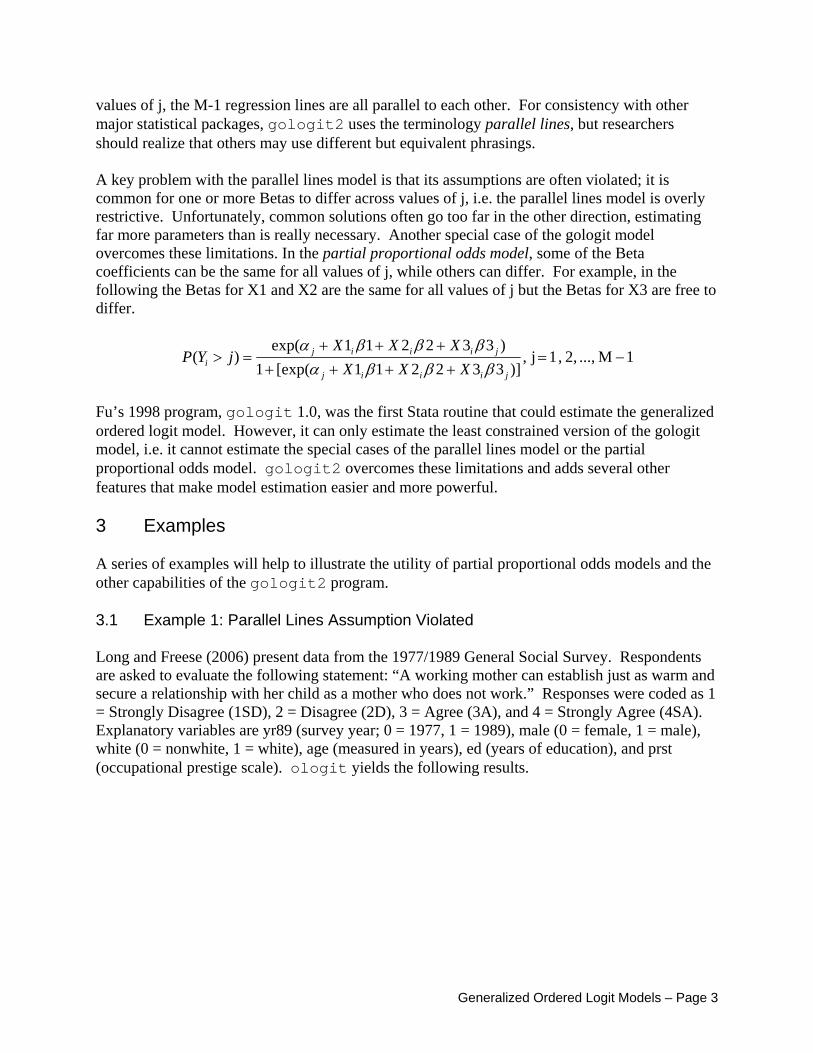
values of j, the M-1 regression lines are all parallel to each other. For consistency with other major statistical packages, gologit2 uses the terminology parallel lines, but researchers should realize that others may use different but equivalent phrasings. A key problem with the parallel lines model is that its assumptions are often violated; it is common for one or more Betas to differ across values of j, i.e. the parallel lines model is overly restrictive. Unfortunately, common solutions often go too far in the other direction, estimating far more parameters than is really necessary. Another special case of the gologit model overcomes these limitations. In the partial proportional odds model, some of the Beta coefficients can be the same for all values of j, while others can differ. For example, in the following the Betas for X1 and X2 are the same for all values of j but the Betas for X3 are free to differ.

1M ..., 2, , 1 j ,)]332211[exp(1

)332211exp()( −=

+++++++

=>jiiij

jiiiji XXX

XXXjYP

βββαβββα

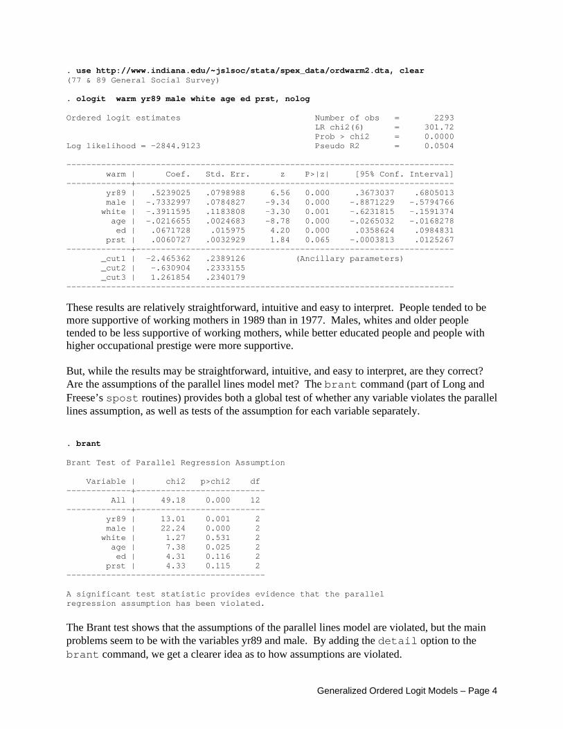
Fu’s 1998 program, gologit 1.0, was the first Stata routine that could estimate the generalized ordered logit model. However, it can only estimate the least constrained version of the gologit model, i.e. it cannot estimate the special cases of the parallel lines model or the partial proportional odds model. gologit2 overcomes these limitations and adds several other features that make model estimation easier and more powerful. 3 Examples A series of examples will help to illustrate the utility of partial proportional odds models and the other capabilities of the gologit2 program. 3.1 Example 1: Parallel Lines Assumption Violated Long and Freese (2006) present data from the 1977/1989 General Social Survey. Respondents are asked to evaluate the following statement: “A working mother can establish just as warm and secure a relationship with her child as a mother who does not work.” Responses were coded as 1 = Strongly Disagree (1SD), 2 = Disagree (2D), 3 = Agree (3A), and 4 = Strongly Agree (4SA). Explanatory variables are yr89 (survey year; 0 = 1977, 1 = 1989), male (0 = female, 1 = male), white (0 = nonwhite, 1 = white), age (measured in years), ed (years of education), and prst (occupational prestige scale). ologit yields the following results.


. use http://www.indiana.edu/~jslsoc/stata/spex_data/ordwarm2.dta, clear (77 & 89 General Social Survey) . ologit warm yr89 male white age ed prst, nolog Ordered logit estimates Number of obs = 2293 LR chi2(6) = 301.72 Prob > chi2 = 0.0000 Log likelihood = -2844.9123 Pseudo R2 = 0.0504 ------------------------------------------------------------------------------ warm | Coef. Std. Err. z P>|z| [95% Conf. Interval] -------------+---------------------------------------------------------------- yr89 | .5239025 .0798988 6.56 0.000 .3673037 .6805013 male | -.7332997 .0784827 -9.34 0.000 -.8871229 -.5794766 white | -.3911595 .1183808 -3.30 0.001 -.6231815 -.1591374 age | -.0216655 .0024683 -8.78 0.000 -.0265032 -.0168278 ed | .0671728 .015975 4.20 0.000 .0358624 .0984831 prst | .0060727 .0032929 1.84 0.065 -.0003813 .0125267 -------------+---------------------------------------------------------------- _cut1 | -2.465362 .2389126 (Ancillary parameters) _cut2 | -.630904 .2333155 _cut3 | 1.261854 .2340179 ------------------------------------------------------------------------------

These results are relatively straightforward, intuitive and easy to interpret. People tended to be more supportive of working mothers in 1989 than in 1977. Males, whites and older people tended to be less supportive of working mothers, while better educated people and people with higher occupational prestige were more supportive. But, while the results may be straightforward, intuitive, and easy to interpret, are they correct? Are the assumptions of the parallel lines model met? The brant command (part of Long and Freese’s spost routines) provides both a global test of whether any variable violates the parallel lines assumption, as well as tests of the assumption for each variable separately. . brant Brant Test of Parallel Regression Assumption Variable | chi2 p>chi2 df -------------+-------------------------- All | 49.18 0.000 12 -------------+-------------------------- yr89 | 13.01 0.001 2 male | 22.24 0.000 2 white | 1.27 0.531 2 age | 7.38 0.025 2 ed | 4.31 0.116 2 prst | 4.33 0.115 2 ---------------------------------------- A significant test statistic provides evidence that the parallel regression assumption has been violated.

The Brant test shows that the assumptions of the parallel lines model are violated, but the main problems seem to be with the variables yr89 and male. By adding the detail option to the brant command, we get a clearer idea as to how assumptions are violated.


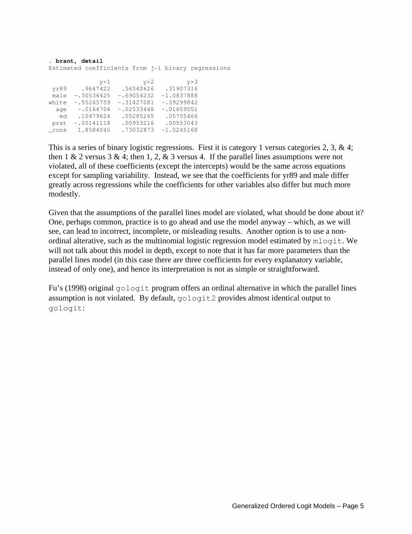
. brant, detail Estimated coefficients from j-1 binary regressions y>1 y>2 y>3 yr89 .9647422 .56540626 .31907316 male -.30536425 -.69054232 -1.0837888 white -.55265759 -.31427081 -.39299842 age -.0164704 -.02533448 -.01859051 ed .10479624 .05285265 .05755466 prst -.00141118 .00953216 .00553043 _cons 1.8584045 .73032873 -1.0245168 This is a series of binary logistic regressions. First it is category 1 versus categories 2, 3, & 4; then 1 & 2 versus 3 & 4; then 1, 2, & 3 versus 4. If the parallel lines assumptions were not violated, all of these coefficients (except the intercepts) would be the same across equations except for sampling variability. Instead, we see that the coefficients for yr89 and male differ greatly across regressions while the coefficients for other variables also differ but much more modestly. Given that the assumptions of the parallel lines model are violated, what should be done about it? One, perhaps common, practice is to go ahead and use the model anyway – which, as we will see, can lead to incorrect, incomplete, or misleading results. Another option is to use a non-ordinal alterative, such as the multinomial logistic regression model estimated by mlogit. We will not talk about this model in depth, except to note that it has far more parameters than the parallel lines model (in this case there are three coefficients for every explanatory variable, instead of only one), and hence its interpretation is not as simple or straightforward. Fu’s (1998) original gologit program offers an ordinal alternative in which the parallel lines assumption is not violated. By default, gologit2 provides almost identical output to gologit:


. gologit2 warm yr89 male white age ed prst Generalized Ordered Logit Estimates Number of obs = 2293 LR chi2(18) = 350.92 Prob > chi2 = 0.0000 Log likelihood = -2820.311 Pseudo R2 = 0.0586 ------------------------------------------------------------------------------ warm | Coef. Std. Err. z P>|z| [95% Conf. Interval] -------------+---------------------------------------------------------------- 1SD | yr89 | .95575 .1547185 6.18 0.000 .6525074 1.258993 male | -.3009776 .1287712 -2.34 0.019 -.5533645 -.0485906 white | -.5287268 .2278446 -2.32 0.020 -.9752941 -.0821595 age | -.0163486 .0039508 -4.14 0.000 -.0240921 -.0086051 ed | .1032469 .0247377 4.17 0.000 .0547619 .151732 prst | -.0016912 .0055997 -0.30 0.763 -.0126665 .009284 _cons | 1.856951 .3872576 4.80 0.000 1.09794 2.615962 -------------+---------------------------------------------------------------- 2D | yr89 | .5363707 .0919074 5.84 0.000 .3562355 .716506 male | -.717995 .0894852 -8.02 0.000 -.8933827 -.5426072 white | -.349234 .1391882 -2.51 0.012 -.6220379 -.07643 age | -.0249764 .0028053 -8.90 0.000 -.0304747 -.0194782 ed | .0558691 .0183654 3.04 0.002 .0198737 .0918646 prst | .0098476 .0038216 2.58 0.010 .0023575 .0173377 _cons | .7198119 .265235 2.71 0.007 .1999609 1.239663 -------------+---------------------------------------------------------------- 3A | yr89 | .3312184 .1127882 2.94 0.003 .1101577 .5522792 male | -1.085618 .1217755 -8.91 0.000 -1.324294 -.8469423 white | -.3775375 .1568429 -2.41 0.016 -.684944 -.070131 age | -.0186902 .0037291 -5.01 0.000 -.025999 -.0113814 ed | .0566852 .0251836 2.25 0.024 .0073263 .1060441 prst | .0049225 .0048543 1.01 0.311 -.0045918 .0144368 _cons | -1.002225 .3446354 -2.91 0.004 -1.677698 -.3267523 ------------------------------------------------------------------------------

Note that the default gologit2 results are very similar to the series of binary logistic regressions estimated by the brant command and can be interpreted the same way, i.e. the first panel contrasts category 1 with categories 2, 3 & 4, the second panel contrasts categories 1 & 2 with categories 3 & 4, and the third panel contrasts categories 1, 2 & 3 with category 42. Hence, positive coefficients indicate that higher values on the explanatory variable make it more likely that the respondent will be in a higher category of Y than the current one, while negative coefficients indicate that higher values on the explanatory variable increase the likelihood of being in the current or a lower category. The main problem with the mlogit and the default gologit/gologit2 models is that they include many more parameters than ologit, possibly many more than is necessary. This is because these methods free all variables from the parallel lines constraint, even though the assumption may only be violated by one or a few of them. gologit2 can overcome this 2 Put another way, the jth panel gives results that are equivalent to a logistic regression in which categories 1 through j have been recoded to 0 and categories j+1 through M have been recoded to 1. The simultaneous estimation of all equations causes results to differ slightly from when each equation is estimated separately. When interpreting results for each panel, it is important to keep in mind that the current category of Y, as well as the lower-coded categories, are serving as the reference group.


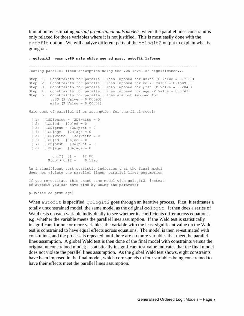
limitation by estimating partial proportional odds models, where the parallel lines constraint is only relaxed for those variables where it is not justified. This is most easily done with the autofit option. We will analyze different parts of the gologit2 output to explain what is going on. . gologit2 warm yr89 male white age ed prst, autofit lrforce ------------------------------------------------------------------------------ Testing parallel lines assumption using the .05 level of significance... Step 1: Constraints for parallel lines imposed for white (P Value = 0.7136) Step 2: Constraints for parallel lines imposed for ed (P Value = 0.1589) Step 3: Constraints for parallel lines imposed for prst (P Value = 0.2046) Step 4: Constraints for parallel lines imposed for age (P Value = 0.0743) Step 5: Constraints for parallel lines are not imposed for yr89 (P Value = 0.00093) male (P Value = 0.00002) Wald test of parallel lines assumption for the final model: ( 1) [1SD]white - [2D]white = 0 ( 2) [1SD]ed - [2D]ed = 0 ( 3) [1SD]prst - [2D]prst = 0 ( 4) [1SD]age - [2D]age = 0 ( 5) [1SD]white - [3A]white = 0 ( 6) [1SD]ed - [3A]ed = 0 ( 7) [1SD]prst - [3A]prst = 0 ( 8) [1SD]age - [3A]age = 0 chi2( 8) = 12.80 Prob > chi2 = 0.1190 An insignificant test statistic indicates that the final model does not violate the parallel lines/ parallel lines assumption If you re-estimate this exact same model with gologit2, instead of autofit you can save time by using the parameter pl(white ed prst age)

When autofit is specified, gologit2 goes through an iterative process. First, it estimates a totally unconstrained model, the same model as the original gologit. It then does a series of Wald tests on each variable individually to see whether its coefficients differ across equations, e.g. whether the variable meets the parallel lines assumption. If the Wald test is statistically insignificant for one or more variables, the variable with the least significant value on the Wald test is constrained to have equal effects across equations. The model is then re-estimated with constraints, and the process is repeated until there are no more variables that meet the parallel lines assumption. A global Wald test is then done of the final model with constraints versus the original unconstrained model; a statistically insignificant test value indicates that the final model does not violate the parallel lines assumption. As the global Wald test shows, eight constraints have been imposed in the final model, which corresponds to four variables being constrained to have their effects meet the parallel lines assumption.


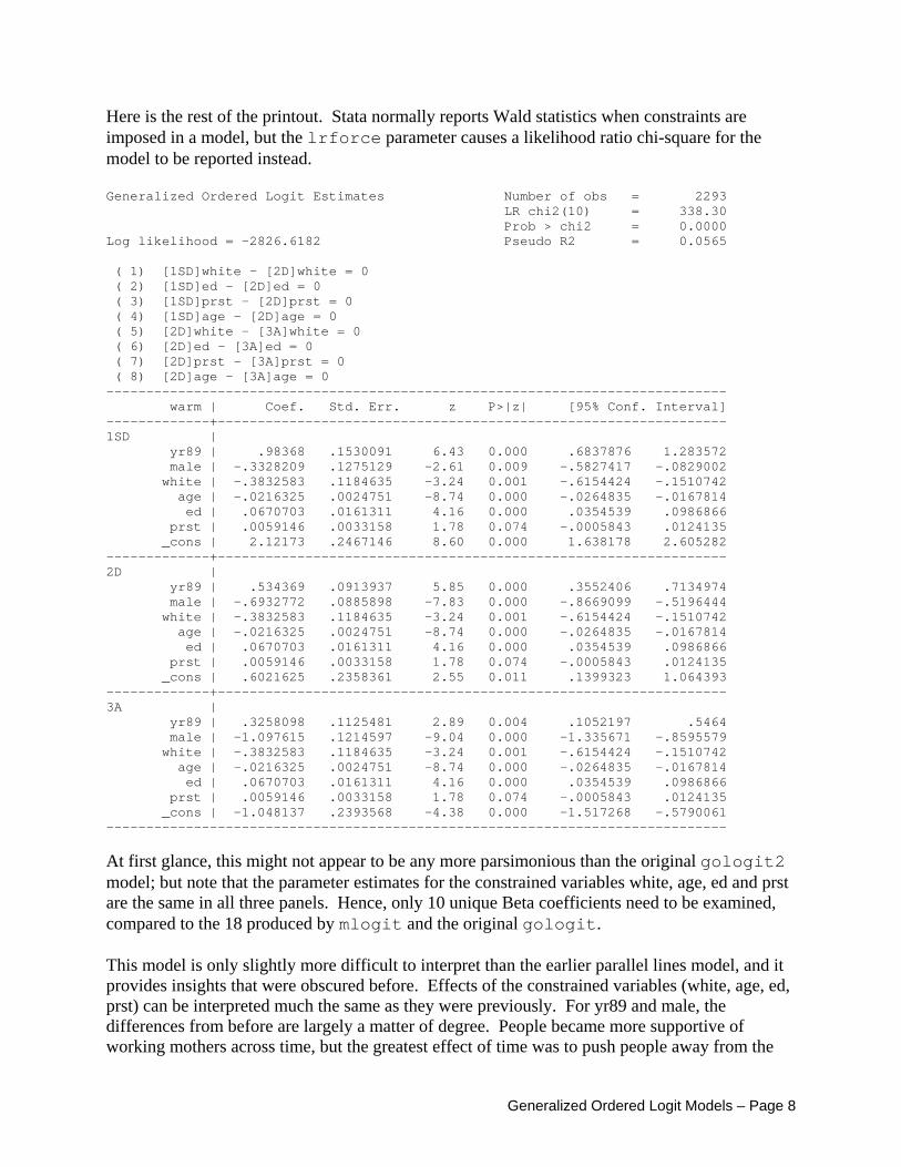
Here is the rest of the printout. Stata normally reports Wald statistics when constraints are imposed in a model, but the lrforce parameter causes a likelihood ratio chi-square for the model to be reported instead. Generalized Ordered Logit Estimates Number of obs = 2293 LR chi2(10) = 338.30 Prob > chi2 = 0.0000 Log likelihood = -2826.6182 Pseudo R2 = 0.0565 ( 1) [1SD]white - [2D]white = 0 ( 2) [1SD]ed - [2D]ed = 0 ( 3) [1SD]prst - [2D]prst = 0 ( 4) [1SD]age - [2D]age = 0 ( 5) [2D]white - [3A]white = 0 ( 6) [2D]ed - [3A]ed = 0 ( 7) [2D]prst - [3A]prst = 0 ( 8) [2D]age - [3A]age = 0 ------------------------------------------------------------------------------ warm | Coef. Std. Err. z P>|z| [95% Conf. Interval] -------------+---------------------------------------------------------------- 1SD | yr89 | .98368 .1530091 6.43 0.000 .6837876 1.283572 male | -.3328209 .1275129 -2.61 0.009 -.5827417 -.0829002 white | -.3832583 .1184635 -3.24 0.001 -.6154424 -.1510742 age | -.0216325 .0024751 -8.74 0.000 -.0264835 -.0167814 ed | .0670703 .0161311 4.16 0.000 .0354539 .0986866 prst | .0059146 .0033158 1.78 0.074 -.0005843 .0124135 _cons | 2.12173 .2467146 8.60 0.000 1.638178 2.605282 -------------+---------------------------------------------------------------- 2D | yr89 | .534369 .0913937 5.85 0.000 .3552406 .7134974 male | -.6932772 .0885898 -7.83 0.000 -.8669099 -.5196444 white | -.3832583 .1184635 -3.24 0.001 -.6154424 -.1510742 age | -.0216325 .0024751 -8.74 0.000 -.0264835 -.0167814 ed | .0670703 .0161311 4.16 0.000 .0354539 .0986866 prst | .0059146 .0033158 1.78 0.074 -.0005843 .0124135 _cons | .6021625 .2358361 2.55 0.011 .1399323 1.064393 -------------+---------------------------------------------------------------- 3A | yr89 | .3258098 .1125481 2.89 0.004 .1052197 .5464 male | -1.097615 .1214597 -9.04 0.000 -1.335671 -.8595579 white | -.3832583 .1184635 -3.24 0.001 -.6154424 -.1510742 age | -.0216325 .0024751 -8.74 0.000 -.0264835 -.0167814 ed | .0670703 .0161311 4.16 0.000 .0354539 .0986866 prst | .0059146 .0033158 1.78 0.074 -.0005843 .0124135 _cons | -1.048137 .2393568 -4.38 0.000 -1.517268 -.5790061 ------------------------------------------------------------------------------

At first glance, this might not appear to be any more parsimonious than the original gologit2 model; but note that the parameter estimates for the constrained variables white, age, ed and prst are the same in all three panels. Hence, only 10 unique Beta coefficients need to be examined, compared to the 18 produced by mlogit and the original gologit. This model is only slightly more difficult to interpret than the earlier parallel lines model, and it provides insights that were obscured before. Effects of the constrained variables (white, age, ed, prst) can be interpreted much the same as they were previously. For yr89 and male, the differences from before are largely a matter of degree. People became more supportive of working mothers across time, but the greatest effect of time was to push people away from the


most extremely negative attitudes. For gender, men were less supportive of working mothers than were women, but they were especially unlikely to have strongly favorable attitudes. Hence, the strongest effects of both gender and time were found with the most extreme attitudes. With the partial proportional odds model estimated by gologit2, the effects of the variables that meet the parallel lines assumption are easily interpretable (you interpret them the same way as you do in ologit). For other variables, an examination of the pattern of coefficients reveals insights that would be obscured or distorted if a parallel lines model were estimated instead. An mlogit or gologit 1.0 analysis might lead to similar conclusions as gologit2 but there would be many more parameters to look at, and the increased number of parameters could cause some effects to become statistically insignificant. While convenient, the autofit option should be used with caution. autofit basically employs a backwards stepwise selection procedure, starting with the least parsimonious model and gradually imposing constraints. As such, it has many of the same strengths and weaknesses as backwards stepwise regression. Researchers may have little theory as to which variables will violate the parallel lines assumptions. The autofit option therefore provides an empirical means of identifying where assumptions may be violated. At the same time, like other stepwise procedures, autofit can capitalize on chance, i.e. just by chance alone some variables may appear to violate the parallel lines assumption when in reality they do not. Ideally, theory should be used when testing violations of assumptions. But, when theory is lacking, an alternative approach is to use more stringent significance levels when testing. Since several tests are being conducted, researchers may wish to specify a more stringent significance level, e.g. .01, or else do something like a Bonferroni or Sidak adjustment. By default, autofit uses the .05 level of significance, but this can be changed, e.g. you can specify autofit(.01). Sample size may also be a factor when choosing a significance level, e.g. in a very large sample even substantively trivial violations of the parallel lines assumption can be statistically significant. Note that, in the above example, the parallel lines constraints for yr89 and male would be rejected even at the .001 level of significance, suggesting we can have confidence in the final model. As always, when choosing a significance level, the costs of Type I versus Type II error need to be considered. A key advantage of gologit2 is that it gives the researcher greater flexibility in choosing between Type I versus Type II error, i.e. the researcher is not forced to choose only between a model where all parameters are constrained versus a model where there are no constraints. Later, we provide examples of alternatives to autofit that the researcher may wish to employ. These options allow for a more theory-based model selection and/or alternative statistical tests for violations of assumptions.


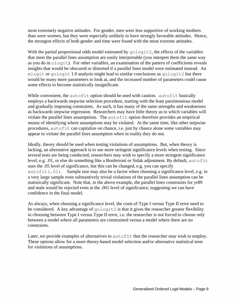
3.2 Example 2: The Alternative Gamma Parameterization Peterson & Harrell (1990) and Lall et al (2002) present an equivalent parameterization of the gologit model, called the Unconstrained Partial Proportional Odds Model3. Under the Peterson/Harrell parameterization, each explanatory variable has • One β coefficient • M – 2 γ coefficients, where M = the number of categories in the Y variable and the γ

coefficients represent deviations from proportionality. The gamma option of gologit2 (abbreviated g) presents this parameterization. . gologit2 warm yr89 male white age ed prst, autofit lrforce gamma Alternative parameterization: Gammas are deviations from proportionality ------------------------------------------------------------------------------ warm | Coef. Std. Err. z P>|z| [95% Conf. Interval] -------------+---------------------------------------------------------------- Beta | yr89 | .98368 .1530091 6.43 0.000 .6837876 1.283572 male | -.3328209 .1275129 -2.61 0.009 -.5827417 -.0829002 white | -.3832583 .1184635 -3.24 0.001 -.6154424 -.1510742 age | -.0216325 .0024751 -8.74 0.000 -.0264835 -.0167814 ed | .0670703 .0161311 4.16 0.000 .0354539 .0986866 prst | .0059146 .0033158 1.78 0.074 -.0005843 .0124135 -------------+---------------------------------------------------------------- Gamma_2 | yr89 | -.449311 .1465627 -3.07 0.002 -.7365686 -.1620533 male | -.3604562 .1233732 -2.92 0.003 -.6022633 -.1186492 -------------+---------------------------------------------------------------- Gamma_3 | yr89 | -.6578702 .1768034 -3.72 0.000 -1.004399 -.3113418 male | -.7647937 .1631536 -4.69 0.000 -1.084569 -.4450186 -------------+---------------------------------------------------------------- Alpha | _cons_1 | 2.12173 .2467146 8.60 0.000 1.638178 2.605282 _cons_2 | .6021625 .2358361 2.55 0.011 .1399323 1.064393 _cons_3 | -1.048137 .2393568 -4.38 0.000 -1.517268 -.5790061 ------------------------------------------------------------------------------

The relationship between the two parameterizations is straightforward. The coefficients for the first equation in the default parameterization correspond to the β’s in the γ parameterization. Gamma_2 parameters = Equation 2 – Equation 1 parameters and Gamma_3 parameters = Equation 3 – Equation 1 parameters. For example in the “Agree” panel for the default parameterization the coefficient for yr89 is .3258098, and in the “Strongly Disagree” panel it is .98368. Gamma_3 for yr89 therefore equals .3258098 - .98368= -.6578702 . You see Gammas only for variables that are not constrained to meet the parallel lines assumption, because the Gammas that are not reported all equal 0.

3 As the name implies, there is also a constrained partial proportional odds model, but the constraints are generally specified by the researcher based on prior knowledge or beliefs. I am not aware of any software that will actually estimate the constraints.


There are several advantages to the γ parameterization: • It is consistent with other published research. • It has a more parsimonious layout – you do not keep seeing the same parameters over and

over that have been constrained to be equal • It provides an alternative way of understanding the parallel lines assumption. If the

Gammas for a variable all equal 0, the assumption is met for that variable, and if all the Gammas equal 0 you have ologit’s parallel lines model.

• By examining the Gammas you can better pinpoint where assumptions are being violated. Normally, all the M-2 Gammas for a variable are either free or else constrained to equal zero, but by using the constraints option (see example 8 below) it is possible to deal with Gammas individually.

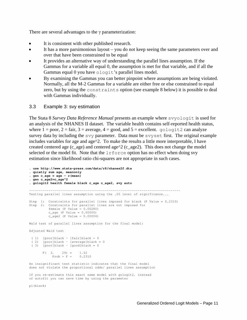
3.3 Example 3: svy estimation The Stata 8 Survey Data Reference Manual presents an example where svyologit is used for an analysis of the NHANES II dataset. The variable health contains self-reported health status, where 1 = poor, 2 = fair, 3 = average, 4 = good, and 5 = excellent. gologit2 can analyze survey data by including the svy parameter. Data must be svyset first. The original example includes variables for age and age^2. To make the results a little more interpretable, I have created centered age (c_age) and centered age^2 (c_age2). This does not change the model selected or the model fit. Note that the lrforce option has no effect when doing svy estimation since likelihood ratio chi-squares are not appropriate in such cases. . use http://www.stata-press.com/data/r8/nhanes2f.dta . quietly sum age, meanonly . gen c_age = age - r(mean) . gen c_age2=c_age^2 . gologit2 health female black c_age c_age2, svy auto ------------------------------------------------------------------------------ Testing parallel lines assumption using the .05 level of significance... Step 1: Constraints for parallel lines imposed for black (P Value = 0.2310) Step 2: Constraints for parallel lines are not imposed for female (P Value = 0.00280) c_age (P Value = 0.00000) c_age2 (P Value = 0.00004) Wald test of parallel lines assumption for the final model: Adjusted Wald test ( 1) [poor]black - [fair]black = 0 ( 2) [poor]black - [average]black = 0 ( 3) [poor]black - [good]black = 0 F( 3, 29) = 1.52 Prob > F = 0.2310 An insignificant test statistic indicates that the final model does not violate the proportional odds/ parallel lines assumption If you re-estimate this exact same model with gologit2, instead of autofit you can save time by using the parameter pl(black)


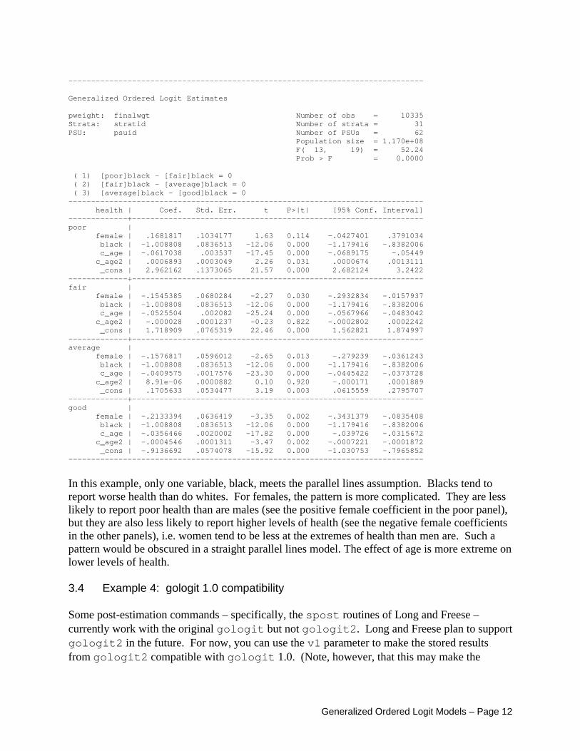
------------------------------------------------------------------------------ Generalized Ordered Logit Estimates pweight: finalwgt Number of obs = 10335 Strata: stratid Number of strata = 31 PSU: psuid Number of PSUs = 62 Population size = 1.170e+08 F( 13, 19) = 52.24 Prob > F = 0.0000 ( 1) [poor]black - [fair]black = 0 ( 2) [fair]black - [average]black = 0 ( 3) [average]black - [good]black = 0 ------------------------------------------------------------------------------ health | Coef. Std. Err. t P>|t| [95% Conf. Interval] -------------+---------------------------------------------------------------- poor | female | .1681817 .1034177 1.63 0.114 -.0427401 .3791034 black | -1.008808 .0836513 -12.06 0.000 -1.179416 -.8382006 c_age | -.0617038 .003537 -17.45 0.000 -.0689175 -.05449 c_age2 | .0006893 .0003049 2.26 0.031 .0000674 .0013111 _cons | 2.962162 .1373065 21.57 0.000 2.682124 3.2422 -------------+---------------------------------------------------------------- fair | female | -.1545385 .0680284 -2.27 0.030 -.2932834 -.0157937 black | -1.008808 .0836513 -12.06 0.000 -1.179416 -.8382006 c_age | -.0525504 .002082 -25.24 0.000 -.0567966 -.0483042 c_age2 | -.000028 .0001237 -0.23 0.822 -.0002802 .0002242 _cons | 1.718909 .0765319 22.46 0.000 1.562821 1.874997 -------------+---------------------------------------------------------------- average | female | -.1576817 .0596012 -2.65 0.013 -.279239 -.0361243 black | -1.008808 .0836513 -12.06 0.000 -1.179416 -.8382006 c_age | -.0409575 .0017576 -23.30 0.000 -.0445422 -.0373728 c_age2 | 8.91e-06 .0000882 0.10 0.920 -.000171 .0001889 _cons | .1705633 .0534477 3.19 0.003 .0615559 .2795707 -------------+---------------------------------------------------------------- good | female | -.2133394 .0636419 -3.35 0.002 -.3431379 -.0835408 black | -1.008808 .0836513 -12.06 0.000 -1.179416 -.8382006 c_age | -.0356466 .0020002 -17.82 0.000 -.039726 -.0315672 c_age2 | -.0004546 .0001311 -3.47 0.002 -.0007221 -.0001872 _cons | -.9136692 .0574078 -15.92 0.000 -1.030753 -.7965852 ------------------------------------------------------------------------------

In this example, only one variable, black, meets the parallel lines assumption. Blacks tend to report worse health than do whites. For females, the pattern is more complicated. They are less likely to report poor health than are males (see the positive female coefficient in the poor panel), but they are also less likely to report higher levels of health (see the negative female coefficients in the other panels), i.e. women tend to be less at the extremes of health than men are. Such a pattern would be obscured in a straight parallel lines model. The effect of age is more extreme on lower levels of health. 3.4 Example 4: gologit 1.0 compatibility Some post-estimation commands – specifically, the spost routines of Long and Freese – currently work with the original gologit but not gologit2. Long and Freese plan to support gologit2 in the future. For now, you can use the v1 parameter to make the stored results from gologit2 compatible with gologit 1.0. (Note, however, that this may make the


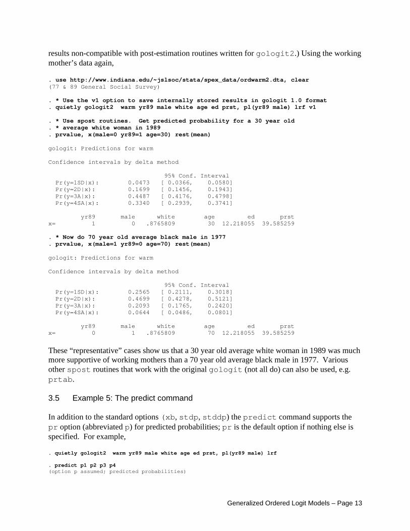
results non-compatible with post-estimation routines written for gologit2.) Using the working mother’s data again, . use http://www.indiana.edu/~jslsoc/stata/spex_data/ordwarm2.dta, clear (77 & 89 General Social Survey) . * Use the v1 option to save internally stored results in gologit 1.0 format . quietly gologit2 warm yr89 male white age ed prst, pl(yr89 male) lrf v1 . * Use spost routines. Get predicted probability for a 30 year old . * average white woman in 1989 . prvalue, x(male=0 yr89=1 age=30) rest(mean) gologit: Predictions for warm Confidence intervals by delta method 95% Conf. Interval Pr(y=1SD|x): 0.0473 [ 0.0366, 0.0580] Pr(y=2D|x): 0.1699 [ 0.1456, 0.1943] Pr(y=3A|x): 0.4487 [ 0.4176, 0.4798] Pr(y=4SA|x): 0.3340 [ 0.2939, 0.3741] yr89 male white age ed prst x= 1 0 .8765809 30 12.218055 39.585259 . * Now do 70 year old average black male in 1977 . prvalue, x(male=1 yr89=0 age=70) rest(mean) gologit: Predictions for warm Confidence intervals by delta method 95% Conf. Interval Pr(y=1SD|x): 0.2565 [ 0.2111, 0.3018] Pr(y=2D|x): 0.4699 [ 0.4278, 0.5121] Pr(y=3A|x): 0.2093 [ 0.1765, 0.2420] Pr(y=4SA|x): 0.0644 [ 0.0486, 0.0801] yr89 male white age ed prst x= 0 1 .8765809 70 12.218055 39.585259

These “representative” cases show us that a 30 year old average white woman in 1989 was much more supportive of working mothers than a 70 year old average black male in 1977. Various other spost routines that work with the original gologit (not all do) can also be used, e.g. prtab. 3.5 Example 5: The predict command In addition to the standard options (xb, stdp, stddp) the predict command supports the pr option (abbreviated p) for predicted probabilities; pr is the default option if nothing else is specified. For example, . quietly gologit2 warm yr89 male white age ed prst, pl(yr89 male) lrf . predict p1 p2 p3 p4 (option p assumed; predicted probabilities)


. list p1 p2 p3 p4 in 1/10 +-------------------------------------------+ | p1 p2 p3 p4 | |-------------------------------------------| 1. | .1083968 .2843347 .4195861 .1876824 | 2. | .2057451 .4859219 .236662 .0716709 | 3. | .1120911 .3004282 .4181407 .16934 | 4. | .2099544 .4283575 .2636952 .0979929 | 5. | .1407257 .3221328 .3887267 .1484148 | |-------------------------------------------| 6. | .2279584 .3338488 .3237104 .1144824 | 7. | .1652819 .3070716 .3804251 .1472214 | 8. | .1100771 .3058248 .4105159 .1735823 | 9. | .0930135 .2593877 .4754793 .1721194 | 10. | .1997068 .3816947 .3235006 .095098 | +-------------------------------------------+

3.6 Example 6: Alternatives to autofit The autofit option provides a convenient means for estimating models that do not violate the parallel lines assumption, but there are other ways that this can be done as well. Rather than use autofit, you can use the pl and npl parameters to specify which variables are or are not constrained to meet the parallel lines assumption. (pl without parameters will produce the same results as ologit, while npl without parameters is the default and produces the same results as the original gologit.) You may want to do this because • you have more control over model specification & testing • if you prefer, you can use Likelihood Ratio, BIC or AIC tests rather than Wald chi-square

tests when deciding on constraints • you have specific hypotheses you want to test about which variables do and do not meet

the parallel lines assumption The store option will cause the command estimates store to be run at the end of the job, making it slightly easier to do LR chi-square contrasts. For example, here is how you could use likelihood ratio chi-square tests to test the model produced by autofit4. . * Least constrained model - same as the original gologit . quietly gologit2 warm yr89 male white age ed prst, store(gologit) . * Partial Proportional Odds Model, estimated using autofit . quietly gologit2 warm yr89 male white age ed prst, store(gologit2) autofit . * ologit clone . quietly gologit2 warm yr89 male white age ed prst, store(ologit) pl . * Confirm that ologit is too restrictive . lrtest ologit gologit Likelihood-ratio test LR chi2(12) = 49.20 (Assumption: ologit nested in gologit) Prob > chi2 = 0.0000

4 The SPSS PLUM test of parallel lines produces results that are identical to the Likelihood Ratio contrast between the ologit and unconstrained gologit models.


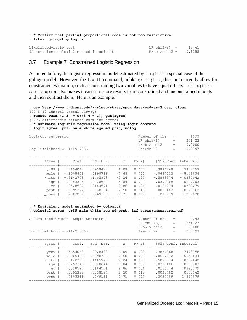
. * Confirm that partial proportional odds is not too restrictive . lrtest gologit gologit2 Likelihood-ratio test LR chi2(8) = 12.61 (Assumption: gologit2 nested in gologit) Prob > chi2 = 0.1258

3.7 Example 7: Constrained Logistic Regression As noted before, the logistic regression model estimated by logit is a special case of the gologit model. However, the logit command, unlike gologit2, does not currently allow for constrained estimation, such as constraining two variables to have equal effects. gologit2’s store option also makes it easier to store results from constrained and unconstrained models and then contrast them. Here is an example: . use http://www.indiana.edu/~jslsoc/stata/spex_data/ordwarm2.dta, clear (77 & 89 General Social Survey) . recode warm (1 2 = 0)(3 4 = 1), gen(agree) (2293 differences between warm and agree) . * Estimate logistic regression model using logit command . logit agree yr89 male white age ed prst, nolog Logistic regression Number of obs = 2293 LR chi2(6) = 251.23 Prob > chi2 = 0.0000 Log likelihood = -1449.7863 Pseudo R2 = 0.0797 ------------------------------------------------------------------------------ agree | Coef. Std. Err. z P>|z| [95% Conf. Interval] -------------+---------------------------------------------------------------- yr89 | .5654063 .0928433 6.09 0.000 .3834368 .7473757 male | -.6905423 .0898786 -7.68 0.000 -.8667012 -.5143834 white | -.3142708 .1405978 -2.24 0.025 -.5898374 -.0387042 age | -.0253345 .0028644 -8.84 0.000 -.0309486 -.0197203 ed | .0528527 .0184571 2.86 0.004 .0166774 .0890279 prst | .0095322 .0038184 2.50 0.013 .0020482 .0170162 _cons | .7303287 .269163 2.71 0.007 .202779 1.257878 ------------------------------------------------------------------------------ . * Equivalent model estimated by gologit2 . gologit2 agree yr89 male white age ed prst, lrf store(unconstrained) Generalized Ordered Logit Estimates Number of obs = 2293 LR chi2(6) = 251.23 Prob > chi2 = 0.0000 Log likelihood = -1449.7863 Pseudo R2 = 0.0797 ------------------------------------------------------------------------------ agree | Coef. Std. Err. z P>|z| [95% Conf. Interval] -------------+---------------------------------------------------------------- yr89 | .5654063 .0928433 6.09 0.000 .3834368 .7473758 male | -.6905423 .0898786 -7.68 0.000 -.8667012 -.5143834 white | -.3142708 .1405978 -2.24 0.025 -.5898374 -.0387042 age | -.0253345 .0028644 -8.84 0.000 -.0309486 -.0197203 ed | .0528527 .0184571 2.86 0.004 .0166774 .0890279 prst | .0095322 .0038184 2.50 0.013 .0020482 .0170162 _cons | .7303288 .269163 2.71 0.007 .2027789 1.257879 ------------------------------------------------------------------------------


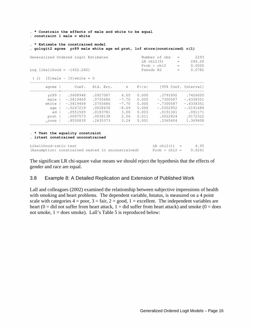
. * Constrain the effects of male and white to be equal

. constraint 1 male = white . * Estimate the constrained model . gologit2 agree yr89 male white age ed prst, lrf store(constrained) c(1) Generalized Ordered Logit Estimates Number of obs = 2293 LR chi2(5) = 246.28 Prob > chi2 = 0.0000 Log likelihood = -1452.2601 Pseudo R2 = 0.0782 ( 1) [0]male - [0]white = 0 ------------------------------------------------------------------------------ agree | Coef. Std. Err. z P>|z| [95% Conf. Interval] -------------+---------------------------------------------------------------- yr89 | .5608948 .0927087 6.05 0.000 .3791892 .7426005 male | -.5819469 .0755686 -7.70 0.000 -.7300587 -.4338351 white | -.5819469 .0755686 -7.70 0.000 -.7300587 -.4338351 age | -.0247219 .0028436 -8.69 0.000 -.0302952 -.0191486 ed | .0551505 .0183781 3.00 0.003 .0191301 .091171 prst | .0097573 .0038138 2.56 0.011 .0022824 .0172322 _cons | .8530839 .2635373 3.24 0.001 .3365604 1.369608 ------------------------------------------------------------------------------ . * Test the equality constraint . lrtest constrained unconstrained Likelihood-ratio test LR chi2(1) = 4.95 (Assumption: constrained nested in unconstrained) Prob > chi2 = 0.0261

The significant LR chi-square value means we should reject the hypothesis that the effects of gender and race are equal. 3.8 Example 8: A Detailed Replication and Extension of Published Work Lall and colleagues (2002) examined the relationship between subjective impressions of health with smoking and heart problems. The dependent variable, hstatus, is measured on a 4 point scale with categories 4 = poor, 3 = fair, 2 = good, 1 = excellent. The independent variables are heart (0 = did not suffer from heart attack, 1 = did suffer from heart attack) and smoke (0 = does not smoke, 1 = does smoke). Lall’s Table 5 is reproduced below:


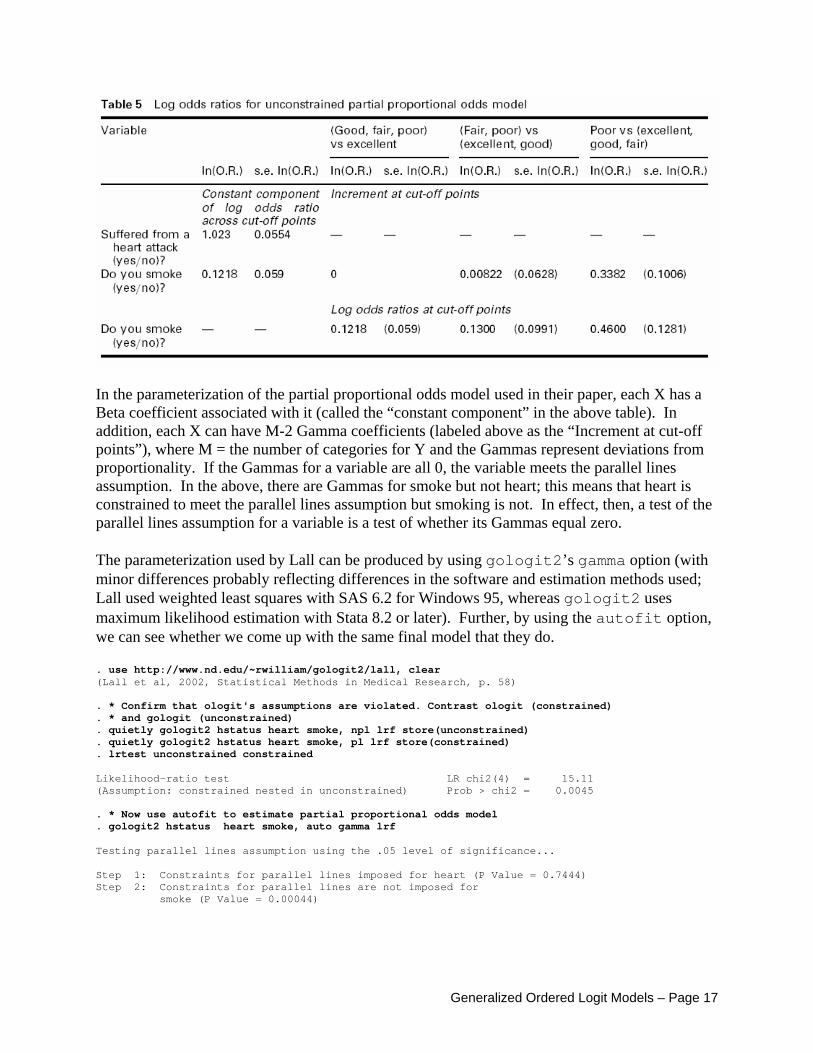
In the parameterization of the partial proportional odds model used in their paper, each X has a Beta coefficient associated with it (called the “constant component” in the above table). In addition, each X can have M-2 Gamma coefficients (labeled above as the “Increment at cut-off points”), where M = the number of categories for Y and the Gammas represent deviations from proportionality. If the Gammas for a variable are all 0, the variable meets the parallel lines assumption. In the above, there are Gammas for smoke but not heart; this means that heart is constrained to meet the parallel lines assumption but smoking is not. In effect, then, a test of the parallel lines assumption for a variable is a test of whether its Gammas equal zero. The parameterization used by Lall can be produced by using gologit2’s gamma option (with minor differences probably reflecting differences in the software and estimation methods used; Lall used weighted least squares with SAS 6.2 for Windows 95, whereas gologit2 uses maximum likelihood estimation with Stata 8.2 or later). Further, by using the autofit option, we can see whether we come up with the same final model that they do. . use http://www.nd.edu/~rwilliam/gologit2/lall, clear (Lall et al, 2002, Statistical Methods in Medical Research, p. 58) . * Confirm that ologit's assumptions are violated. Contrast ologit (constrained) . * and gologit (unconstrained) . quietly gologit2 hstatus heart smoke, npl lrf store(unconstrained) . quietly gologit2 hstatus heart smoke, pl lrf store(constrained) . lrtest unconstrained constrained Likelihood-ratio test LR chi2(4) = 15.11 (Assumption: constrained nested in unconstrained) Prob > chi2 = 0.0045 . * Now use autofit to estimate partial proportional odds model . gologit2 hstatus heart smoke, auto gamma lrf Testing parallel lines assumption using the .05 level of significance... Step 1: Constraints for parallel lines imposed for heart (P Value = 0.7444) Step 2: Constraints for parallel lines are not imposed for smoke (P Value = 0.00044)


Wald test of parallel lines assumption for the final model: ( 1) [Excellent]heart - [Good]heart = 0 ( 2) [Excellent]heart - [Fair]heart = 0 chi2( 2) = 0.59 Prob > chi2 = 0.7444 An insignificant test statistic indicates that the final model does not violate the proportional odds/ parallel lines assumption If you re-estimate this exact same model with gologit2, instead of autofit you can save time by using the parameter pl(heart) ------------------------------------------------------------------------------ Generalized Ordered Logit Estimates Number of obs = 12535 LR chi2(4) = 373.10 Prob > chi2 = 0.0000 Log likelihood = -14664.661 Pseudo R2 = 0.0126 ( 1) [Excellent]heart - [Good]heart = 0 ( 2) [Good]heart - [Fair]heart = 0 ------------------------------------------------------------------------------ hstatus | Coef. Std. Err. z P>|z| [95% Conf. Interval] -------------+---------------------------------------------------------------- Excellent | heart | 1.025339 .0551397 18.60 0.000 .9172672 1.133411 smoke | .127191 .0590098 2.16 0.031 .0115339 .2428482 _cons | 1.303032 .0251244 51.86 0.000 1.253789 1.352275 -------------+---------------------------------------------------------------- Good | heart | 1.025339 .0551397 18.60 0.000 .9172672 1.133411 smoke | .1283844 .0488556 2.63 0.009 .0326292 .2241396 _cons | -.8967713 .0226262 -39.63 0.000 -.9411177 -.8524248 -------------+---------------------------------------------------------------- Fair | heart | 1.025339 .0551397 18.60 0.000 .9172672 1.133411 smoke | .4581369 .0894379 5.12 0.000 .2828418 .633432 _cons | -3.082652 .0463864 -66.46 0.000 -3.173568 -2.991737 ------------------------------------------------------------------------------ Alternative parameterization: Gammas are deviations from proportionality ------------------------------------------------------------------------------ hstatus | Coef. Std. Err. z P>|z| [95% Conf. Interval] -------------+---------------------------------------------------------------- Beta | heart | 1.025339 .0551397 18.60 0.000 .9172672 1.133411 smoke | .127191 .0590098 2.16 0.031 .0115339 .2428482 -------------+---------------------------------------------------------------- Gamma_2 | smoke | .0011933 .0629692 0.02 0.985 -.1222239 .1246106 -------------+---------------------------------------------------------------- Gamma_3 | smoke | .3309459 .100827 3.28 0.001 .1333287 .5285631 -------------+---------------------------------------------------------------- Alpha | _cons_1 | 1.303032 .0251244 51.86 0.000 1.253789 1.352275 _cons_2 | -.8967713 .0226262 -39.63 0.000 -.9411177 -.8524248 _cons_3 | -3.082652 .0463864 -66.46 0.000 -3.173568 -2.991737 ------------------------------------------------------------------------------ Using either parameterization, the results suggest that those who have had heart attacks tend to report worse health. The same is true for smokers, but smokers are especially likely to report themselves as being in poor health as opposed to fair, good or excellent health.


The use of the autofit parameter confirms Lall’s choice of models, i.e. autofit produces the same partial proportional odds model that he and his colleagues reported. But, if we wanted to just trust him, we could have estimated the same model by using the pl or npl parameters. The following two commands will each produce the same results in this case: . gologit2 hstatus heart smoke, pl(heart) gamma lrf . gologit2 hstatus heart smoke, npl(smoke) gamma lrf

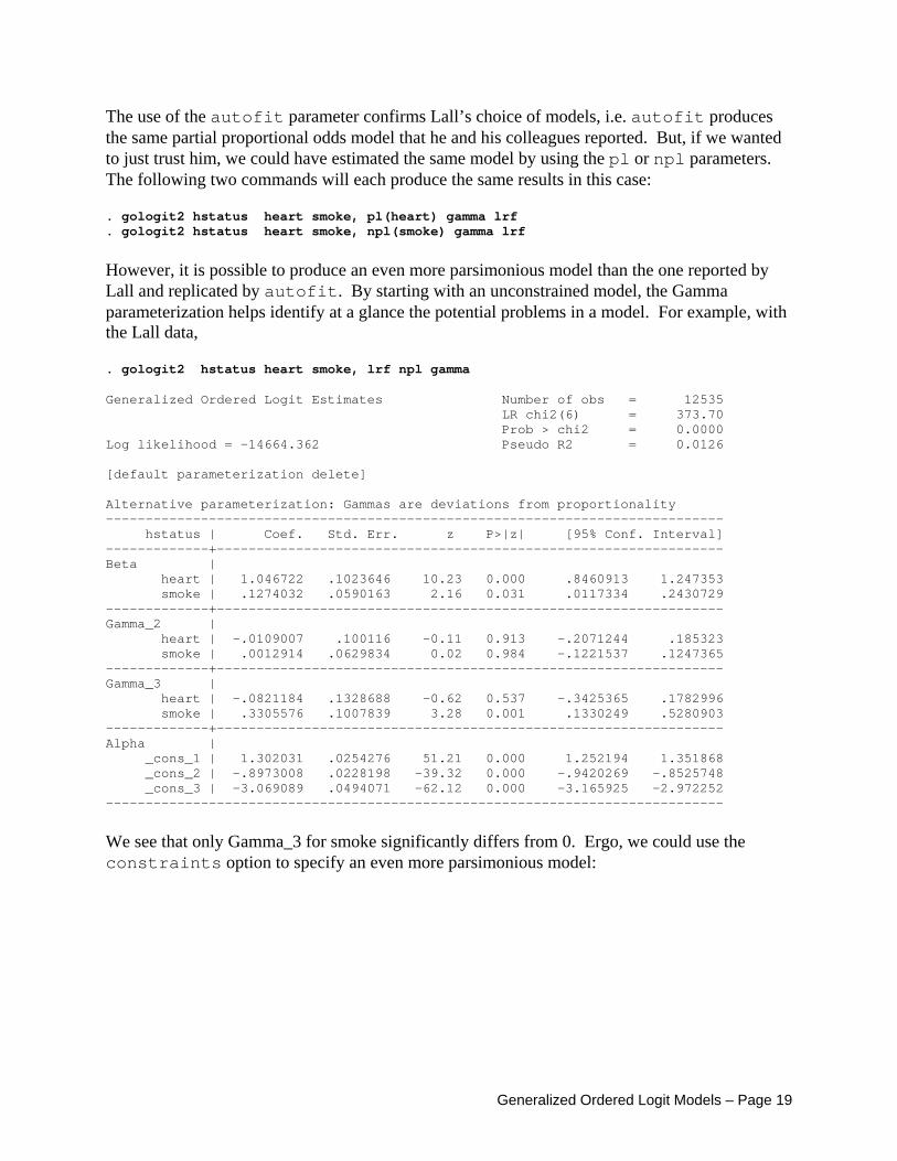
However, it is possible to produce an even more parsimonious model than the one reported by Lall and replicated by autofit. By starting with an unconstrained model, the Gamma parameterization helps identify at a glance the potential problems in a model. For example, with the Lall data, . gologit2 hstatus heart smoke, lrf npl gamma Generalized Ordered Logit Estimates Number of obs = 12535 LR chi2(6) = 373.70 Prob > chi2 = 0.0000 Log likelihood = -14664.362 Pseudo R2 = 0.0126 [default parameterization delete] Alternative parameterization: Gammas are deviations from proportionality ------------------------------------------------------------------------------ hstatus | Coef. Std. Err. z P>|z| [95% Conf. Interval] -------------+---------------------------------------------------------------- Beta | heart | 1.046722 .1023646 10.23 0.000 .8460913 1.247353 smoke | .1274032 .0590163 2.16 0.031 .0117334 .2430729 -------------+---------------------------------------------------------------- Gamma_2 | heart | -.0109007 .100116 -0.11 0.913 -.2071244 .185323 smoke | .0012914 .0629834 0.02 0.984 -.1221537 .1247365 -------------+---------------------------------------------------------------- Gamma_3 | heart | -.0821184 .1328688 -0.62 0.537 -.3425365 .1782996 smoke | .3305576 .1007839 3.28 0.001 .1330249 .5280903 -------------+---------------------------------------------------------------- Alpha | _cons_1 | 1.302031 .0254276 51.21 0.000 1.252194 1.351868 _cons_2 | -.8973008 .0228198 -39.32 0.000 -.9420269 -.8525748 _cons_3 | -3.069089 .0494071 -62.12 0.000 -3.165925 -2.972252 ------------------------------------------------------------------------------

We see that only Gamma_3 for smoke significantly differs from 0. Ergo, we could use the constraints option to specify an even more parsimonious model:


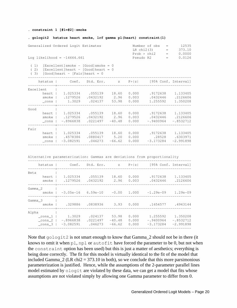
. constraint 1 [#1=#2]:smoke . gologit2 hstatus heart smoke, lrf gamma pl(heart) constraint(1) Generalized Ordered Logit Estimates Number of obs = 12535 LR chi2(3) = 373.10 Prob > chi2 = 0.0000 Log likelihood = -14664.661 Pseudo R2 = 0.0126 ( 1) [Excellent]smoke - [Good]smoke = 0 ( 2) [Excellent]heart - [Good]heart = 0 ( 3) [Good]heart - [Fair]heart = 0 ------------------------------------------------------------------------------ hstatus | Coef. Std. Err. z P>|z| [95% Conf. Interval] -------------+---------------------------------------------------------------- Excellent | heart | 1.025334 .055139 18.60 0.000 .9172638 1.133405 smoke | .1279526 .0432192 2.96 0.003 .0432446 .2126606 _cons | 1.3029 .024137 53.98 0.000 1.255592 1.350208 -------------+---------------------------------------------------------------- Good | heart | 1.025334 .055139 18.60 0.000 .9172638 1.133405 smoke | .1279526 .0432192 2.96 0.003 .0432446 .2126606 _cons | -.8966838 .0221497 -40.48 0.000 -.9400964 -.8532712 -------------+---------------------------------------------------------------- Fair | heart | 1.025334 .055139 18.60 0.000 .9172638 1.133405 smoke | .4578386 .0880417 5.20 0.000 .28528 .6303971 _cons | -3.082591 .046273 -66.62 0.000 -3.173284 -2.991898 ------------------------------------------------------------------------------ Alternative parameterization: Gammas are deviations from proportionality ------------------------------------------------------------------------------ hstatus | Coef. Std. Err. z P>|z| [95% Conf. Interval] -------------+---------------------------------------------------------------- Beta | heart | 1.025334 .055139 18.60 0.000 .9172638 1.133405 smoke | .1279526 .0432192 2.96 0.003 .0432446 .2126606 -------------+---------------------------------------------------------------- Gamma_2 | smoke | -3.05e-16 6.59e-10 -0.00 1.000 -1.29e-09 1.29e-09 -------------+---------------------------------------------------------------- Gamma_3 | smoke | .329886 .0838936 3.93 0.000 .1654577 .4943144 -------------+---------------------------------------------------------------- Alpha | _cons_1 | 1.3029 .024137 53.98 0.000 1.255592 1.350208 _cons_2 | -.8966838 .0221497 -40.48 0.000 -.9400964 -.8532712 _cons_3 | -3.082591 .046273 -66.62 0.000 -3.173284 -2.991898 ------------------------------------------------------------------------------

Note that gologit2 is not smart enough to know that Gamma_2 should not be in there (it knows to omit it when pl, npl or autofit have forced the parameter to be 0, but not when the constraint option has been used) but this is just a matter of aesthetics; everything is being done correctly. The fit for this model is virtually identical to the fit of the model that included Gamma_2 (LR chi2 = 373.10 in both), so we conclude that this more parsimonious parameterization is justified. Hence, while the assumptions of the 2-parameter parallel lines model estimated by ologit are violated by these data, we can get a model that fits whose assumptions are not violated simply by allowing one Gamma parameter to differ from 0.


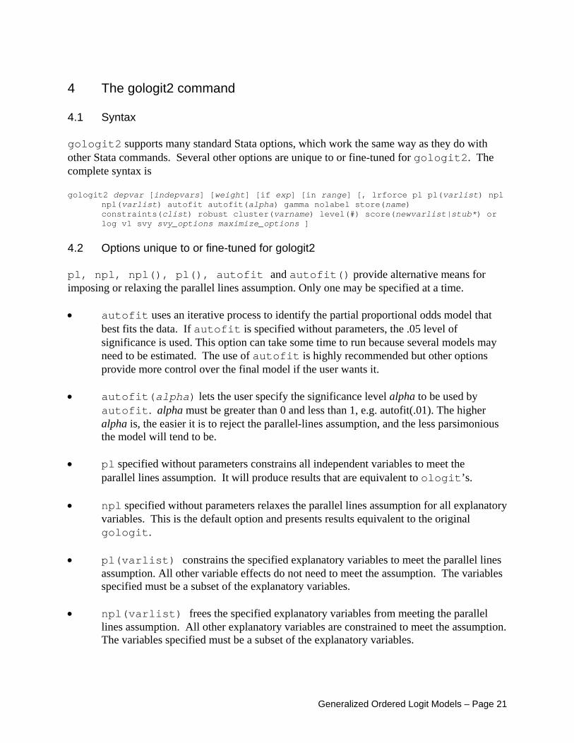
4 The gologit2 command 4.1 Syntax gologit2 supports many standard Stata options, which work the same way as they do with other Stata commands. Several other options are unique to or fine-tuned for gologit2. The complete syntax is gologit2 depvar [indepvars] [weight] [if exp] [in range] [, lrforce pl pl(varlist) npl

npl(varlist) autofit autofit(alpha) gamma nolabel store(name) constraints(clist) robust cluster(varname) level(#) score(newvarlist|stub*) or log v1 svy svy_options maximize_options ]

4.2 Options unique to or fine-tuned for gologit2 pl, npl, npl(), pl(), autofit and autofit() provide alternative means for imposing or relaxing the parallel lines assumption. Only one may be specified at a time. • autofit uses an iterative process to identify the partial proportional odds model that

best fits the data. If autofit is specified without parameters, the .05 level of significance is used. This option can take some time to run because several models may need to be estimated. The use of autofit is highly recommended but other options provide more control over the final model if the user wants it.

• autofit(alpha) lets the user specify the significance level alpha to be used by

autofit. alpha must be greater than 0 and less than 1, e.g. autofit(.01). The higher alpha is, the easier it is to reject the parallel-lines assumption, and the less parsimonious the model will tend to be.

• pl specified without parameters constrains all independent variables to meet the

parallel lines assumption. It will produce results that are equivalent to ologit’s. • npl specified without parameters relaxes the parallel lines assumption for all explanatory

variables. This is the default option and presents results equivalent to the original gologit.

• pl(varlist) constrains the specified explanatory variables to meet the parallel lines

assumption. All other variable effects do not need to meet the assumption. The variables specified must be a subset of the explanatory variables.

• npl(varlist) frees the specified explanatory variables from meeting the parallel

lines assumption. All other explanatory variables are constrained to meet the assumption. The variables specified must be a subset of the explanatory variables.


lrforce forces Stata to report a Likelihood Ratio Statistic under certain conditions when it ordinarily would not. Some types of constraints can make a Likelihood Ratio chi-square test invalid. Hence, to be safe, Stata reports a Wald statistic whenever constraints are used. But, Likelihood Ratio statistics should be correct for the types of constraints imposed by the pl, npl and autofit options. Note that the lrforce option will be ignored when robust standard errors are specified either directly or indirectly, e.g. via use of the robust or svy options. Use this option with caution if you specify other constraints since these may make a LR chi- square statistic inappropriate. gamma displays an alternative but equivalent parameterization of the partial proportional odds model used by Peterson and Harrell (1990) and Lall et al (2002). Under this parameterization, there is one Beta coefficient and M-2 Gamma coefficients for each explanatory variable, where M = the number of categories for Y. The Gammas indicate the extent to which the parallel lines assumption is violated by the variable, i.e. when the Gammas do not significantly differ from 0 the parallel lines assumption is met. Advantages of this parameterization include the fact that it is more parsimonious than the default layout. In addition, by examining the test statistics for the Gammas, you can see where parallel lines assumptions are being violated. store(name) causes the command estimates store name to be executed when gologit2 finishes. This is useful for when you wish to estimate a series of models and want to save the results. nolabel causes the equations to be named eq1, eq2, etc. The default is to use the first 32 characters of the value labels and/or the values of Y as the equation labels. Note that some characters cannot be used in equation names, e.g. the period (.), the dollar sign ($), and the colon(:), and will be replaced with the underscore (_) character. The default behavior works well when the value labels are short and descriptive. It may not work well when value labels are very long and/or include characters that have to be changed to underscores. If the printout looks unattractive and/or you are getting strange errors, try changing the value labels of Y or else use the nolabel option. v1 causes gologit2 to return results in a format that is consistent with gologit 1.0. This may be useful/necessary for post-estimation commands that were written specifically for gologit (in particular, some versions of the Long and Freese spost commands support gologit but not gologit2). However, post-estimation commands written for gologit2 may not work correctly if v1 is specified. log displays the iteration log. By default it is suppressed. or reports the estimated coefficients transformed to relative odds ratios, i.e., exp(b) rather than b; see [R] ologit for a description of this concept. Options rrr, eform, hr and irr produce identical results (labeled differently) and can also be used. constraints(clist) specifies linear constraints to be applied during estimation. Constraints are defined with the constraint command. constraints(1) specifies that


the model is to be constrained according to constraint 1; constraints(1-4) specifies constraints 1 through 4; constraints(1-4,8) specifies 1 through 4 and 8. Keep in mind that the pl, npl and autofit options work by generating across-equation constraints, which may affect how any additional constraints should be specified. When using the constraint command, refer to equations by their equation number, e.g. #1, #2, etc. svy indicates that gologit2 is to pick up the svy settings set by svyset and use the robust variance estimator. Thus, this option requires the data to be svyset; see help svyset. When using svy estimation, use of if or in restrictions will not produce correct variance estimates for subpopulations in many cases. To compute estimates for subpopulations, use the subpop() option. If svy has not been specified, use of other svy-related options (e.g. subpop, deff, meff) will produce an error. 4.3 Other standard Stata options supported by gologit2 robust cluster level score 4.4 Other standard svy-related options supported by gologit2 subpop nosvyadjust prob ci deff deft meff meft 4.5 Options available when replaying results gamma store or level prob ci deff deft prob, ci, deff and deft are only available when svy estimation has been used. 4.6 Options available for the predict command xb stdp stddp p p gives the predicted probability. Note that you specify one new variable with xb, stdp, and stddp and specify either one or M new variables with p. These statistics are available both in and out of sample; type "predict ... if e(sample)" if wanted only for the estimation sample. 5 Support for gologit2 Richard Williams Department of Sociology University of Notre Dame [email protected] http://www.nd.edu/~rwilliam/gologit2/


mailto:[email protected]

http://www.nd.edu/%7Erwilliam/gologit2/

6 Acknowledgements Vincent Kang Fu of the Utah Department of Sociology wrote gologit 1.0 and graciously allowed Richard Williams to incorporate parts of its source code and documentation in gologit2. The documentation for Stata 8.2's mlogit command and the program mlogit_p were major aids in developing the gologit2 documentation and in adding support for the predict command. Much of the code is adapted from Maximum Likelihood Estimation with Stata, Second Edition, by William Gould, Jeffrey Pitblado and William Sribney. Sarah Mustillo, Dan Powers, J. Scott Long, Nick Cox and Kit Baum provided stimulating and helpful comments. 7 References Clogg, Clifford C. and Edward S. Shihadeh. 1994. Statistical Models for Ordinal Variables. Thousand Oaks, CA:

Sage. Fu, Vincent. 1998. sg88: Estimating Generalized Ordered Logit Models. Stata Technical Bulletin 44: 27-30. In

Stata Technical Bulletin Reprints, vol 8, 160-164. College Station, TX: Stata Press. Lall, R., S.J. Walters, K. Morgan, and MRC CFAS Co-operative Institute of Public Health. 2002. A Review of

Ordinal Regression Models Applied on Health-Related Quality of Life Assessments. Statistical Methods in Medical Research 11:49-67.

Long, J. Scott and Jeremy Freese. 2006. Regression Models for Categorical Dependent Variables Using Stata.

Second Edition. College Station, TX: Stata Press. Norusis, Marija. 2005. SPSS 13.0 Advanced Statistical Procedures Companion. Upper Saddle River, New Jersey:

Prentice Hall. Peterson, Bercedis and Frank E. Harrell Jr. 1990. Partial Proportional Odds Models for Ordinal Response

Variables. Applied Statistics 39(2):205-217. SAS Institute Inc. 2004. SAS/STAT 9.1 User’s Guide. Cary, NC: SAS Institute Inc. Wolfe, R. and W.Gould. 1998. An approximate likelihood-ratio test for ordinal response models. Stata Technical

Bulletin 42: 24-27. In Stata Technical Bulletin Reprints, vol 7, 199-204. College Statio, TX: Stata Press. About the Author Richard Williams is Associate Professor and a former Chairman of the Department of Sociology at the University of Notre Dame. His teaching and research interests include Methods and Statistics, Demography, and Urban Sociology. His work has appeared in the American Sociological Review, Social Problems, Demography, Sociology of Education, Journal of Urban Affairs, Cityscape, Journal of Marriage and the Family, and Sociological Methods and Research. His current research, which has been funded by grants from the Department of Housing and Urban Development and the National Science Foundation, focuses on the causes and consequences of inequality in American home ownership. He is a frequent contributor to Statalist.


Documents

Go Log It 2