Embed Size (px)
Citation preview
International Journal of Economic Sciences Vol. III / No. 1 / 2014
12
GMM Estimation and Shapiro-Francia Normality Test:
A Case Study of CEE Economies
Davtyan Azat
ABSTRACT
The present paper estimates the link between GDP per capita, inflation (GDP deflator), exports,
imports, final consumption, gross capital formation, tax revenue and public expense of CEE
countries (Bulgaria, Romania, the Czech Republic, Slovak Republic, Poland, Slovenia and Russia)
using GMM estimation for the period 2005-2010. Besides, we run Shapiro-Francia W test to
indicate the patterns of normal distribution among samples of our study. The objective of this
quantitative empirical is twofold: first, it examines the linkages of economic indicators of CEE
countries in order to find out the main changes of economic landscape. Second, it aims at
highlighting the development of CEE countries on the way of deeper convergence to the euro area
utilizing the available panel series. We find that GDP per capita of CEE countries is in negative
relationship with expense, final consumption, gross capital formation, exports and inflation. With
regard to Shapiro-Francia W test, we assume that variables show a normal distribution.
Keywords: exports; final consumption, Arellano-Bond test; GMM; gross capital formation; imports
JEL classification: E21; E22; H50; E31
Author
Davtyan Azat, West University of Timisoara, Faculty of Economics and Business Administration str.
J. H. Pestalozzi, nr. 16 300115, Timisoara, Romania. Email: [email protected]
Citation Davtyan Azat (2014). GMM Estimation and Shapiro-Francia Normality Test: A Case Study of CEE
Economies. International Journal of Economic Sciences, Vol. III, No. 1/2014, pp. 12-26.
International Journal of Economic Sciences Vol. III / No. 1 / 2014
13
Introduction
The deepening of financial integration in the EU has accelerated in the last decade. The strong trade
relations, growth of foreign investments and capital market development evidence strengthening
financial integration processes. However, the presence of sophisticated market regulation,
information and governance are necessary preconditions to benefit from financial integration.
Smooth and continuous financial integration assumes sustainable exchange rate and interest rate
policies, efficient structural reforms and crucial role of domestic funding. Besides, it is perhaps best
known that the efficient interactions of market participants and stability of capital markets are
crucial to guarantee a smooth and effective transmission of monetary policy.
The cross-border capital flows and penetration of foreign credit institutions are the main outcomes
of financial integration processes. In addition, the prevalence of same rules and asset pricing
mechanisms in markets are considered one of the principles of financial integration. Factors like
portfolio risk diversification due to large financial markets and easier access to capital markets and
funding enhance benefits of market participants and brought more efficient diversification of
investments in the sectors of real economy. Thus, financial integration leads to the expansion of
economy. Besides, deeper financial integration to the euro area leads to a high capital flow
liberalization and increasing role of institutional investors. In this regard, the development of
primary and secondary markets with adequate financial regulation and supervision will enhance the
competitiveness and economic alignment of CEE countries with the euro area.
Financial integration is also conditioned by a number of foreign companies operating in CEE
countries. In this vein, the growing body of foreign companies enhances cross-border fundraising
and economic alignment of CEE region. Moreover, the CEE governments tend to promote law
enforcement, improve business environment and facilitate the entry of foreign companies.
Particularly, reforms directed to increasing the efficiency of absorption of EU funds and the
enlargement of secondary markets will bring a deepening of financial integration.
The CEE countries have a progress in corporate governance and financial supervision which
positively affect securities market development. Other components of capital market (insurance
companies and pension funds) just started to develop. In this regard, state authorities should create
legal bases for the enlargement of this market segment.
So, CEE countries have a great potential to decrease economic imbalances and accelerate financial
integration. Ample opportunities for foreign investments lead to the gradual diversification of
capital flows to corporate securities market and development of private equity activity. This process
fosters the depth of financial markets and mitigates domestic and external risks.
After the accession to the EU foreign direct and portfolio investments in CEE countries
significantly improve economic landscape of this region. Domestic companies and banks started
heavily rely on foreign capital which weakened the role of internal financial markets. Financial
inflows and financial convergence brought high level of interconnectedness between CEE and euro
area countries. Before the onset of crisis, the CEE countries experienced high economic growth
which was conditioned by increasing international trade, restructuring processes in financial sector
and efforts of economic convergence towards euro area countries. The fast growth in mortgage
lending led to the enlargement of banking activity which increased its market positions in different
spheres. In addition, financial supervision measures and legal reforms regulate market environment
and create necessary conditions for the growth of foreign investments.
The CEE capital markets are characterized by a high ownership of foreign banks. This can be
explained by large FDI inflows before the financial turmoil. Hence, the high market concentration
of CEE countries and prevalence of banks make those economies more volatile to external shocks.
In this context, the significant exposure of CEE financial systems to foreign banking sectors
heightens the need to increase financial buffers. This action is imperative as for further financial
integration and overcoming financial disturbances as well.
International Journal of Economic Sciences Vol. III / No. 1 / 2014
14
The real convergence in GDP per capita, price levels and interest rates provide a platform for
joining the euro area. CEE countries benefit from deepening trade relations improving domestic
business environment. Thus, continuous economic alignment provides new opportunities for
economic growth. In addition, the convergence of monetary policy and prudential regulation aim at
enhancing financial stability. In this regard, the strains of CEE countries are directed to carry out
macroeconomic and financial reforms to provide high economic growth and decrease public debt.
The study of driving factors of CEE financial integration is crucial in terms of possible entry of
CEE countries to the euro area. In particular, the current account deficit has a significant impact on
financial integration because it reflects investment flows of the country. Another factor is the trade
openness which facilitates capital flows among euro area and CEE countries and, therefore, fosters
financial integration.
CEE countries have a different potential for economic development and improvement of business
environment. This is mainly conditioned by the effectiveness of privatization process, ownership
structure and institutional framework. In particular, the share of corporate sector (Slovenia, Poland
and Hungary) in capital market is visibly significant owing to the efficiency of privatization. Unlike
Romania and Bulgaria high diversification of equity markets in Hungary, the Czech Republic and
Poland allows increase foreign investments. On the other hand, the establishment of CEE Stock
Exchange Group (CEESEG) aims at strengthening cooperation between Hungarian, Slovenian,
Czech and Austrian stock markets. This brings an improvement of trading platforms and growth of
market capitalization of listed companies.
The economic performance of CEE countries changed during the financial turmoil. As a result of
the crisis macroeconomic situation in CEE region worsened because international funding became
too expensive, external debt increased and non-performing loans of banks grew significantly. The
activity of foreign subsidiaries worsened which was conditioned by deteriorating funding
conditions. Moreover, a sharp decline of lending and asset quality hindered financial performance.
In current global financial turbulences the strong financial supervision and prudential regulation is
considered the primary issue for CEE countries. There is a need to decrease the risks from currency
appreciation, credit crunch and current account deficits. In addition, the structure of financial
markets and shareholding should be changed in order to increase the share of domestic market
participants. On the other hand, the effective cooperation with international financial organizations
can foster the coordination of foreign trade, development of financial infrastructure and open new
opportunities for business activity.
It is clear that after the financial crisis CEE countries registered different levels of inflation which
were conditioned by the speed of economic recovery. In this vein, Romania, Bulgaria and the Czech
Republic showed high resilience to changes of global commodity prices. On the other hand,
inflation pressures in Hungary worsened the current account positions of this country. Moreover, the
high inflation accompanied with the large foreign currency lending and sharp drop in domestic
demand deteriorate economic growth of Hungary and Bulgaria. Those countries need to strengthen
their policy adjustments in the foreign currency lending, improve capital relocation among
economic sectors and carry out development-oriented fiscal policy.
Taking into account the current developments of CEE economies this paper aims to identify the
main correlation patterns between economic indicators of those countries. The next section covers
the literature review indicating different works considering the relationships between investments,
public expense, current account balance, inflation, final consumption and tax revenue. The second
section includes the empirical methodology identifying the features and advantages of Arellano-
Bond/Arellano-Bover estimation and Shapiro-Francia normality test. The last section concludes.
International Journal of Economic Sciences Vol. III / No. 1 / 2014
15
1. Literature review
The relationships between exports, investments, imports, government expense, taxes and
government expense, and etc were investigated by many researchers. Particularly, Collins and Ofair
(1997) assume that the economic growth is conditioned by gross capital formation and real
exchange rate. They highlight the negative impact of exchange rate volatility and suppose a strong
relationship between high overvaluation and GDP growth. Other authors like Rodrick (2007) and
Aguirre and Calderon (2006) conduct a large research in this field. A more fundamental role of
exchange rate policy was proved by Rodrick (2007). The negative and significant correlation
between the real exchange rate misalignment and economic growth has been declared by Aguirre
and Calderon (2006). Cottani et al., (1990) and Bleany and Greenaway (2001) also investigate the
influence of direct and portfolio investments and export growth on the GDP.
Works by Mundell (1957) and Willamson (1975) and Markusen and Venables (1995) emphasize the
main factors affecting FDI and exports. Turkan (2006) shows a negative relation between FDI and
trade in final goods for the USA market. Jenkins and Thomas (2002) highlight the role of FDI on
economic output.
Asiedu (2002 and 2006) suppose that changes in taxation have a different influence on gross capital
formation of developing countries that even within developing countries tax effects on FDI might
be different in sub-Saharan Africa. Tanzi (1987) shows that overvaluation has a directly impact the
balance sheet of a country. He also indicates the crucial role of exchange rate policy and tax
revenue. Jong-Wha Lee (1995) found that direct and portfolio investments is one of the main factors
of economic growth.
Using a panel of 27 countries from Africa, Asia and the Western Hemisphere, covering the period
1980 to 1992 and a panel of 105 countries, spanning 1980 to 1995, Ebrill et al. (1999) examine two
complementary models of the determinants of import and international trade tax revenue. Using a
fixed-effects and an instrumental regression framework they conclude that tariff reforms do not,
necessarily lead to lower trade tax revenue. They find that, in both models, depreciation of the
exchange rate is significantly linked to higher trade tax revenues, confirming Tanzi’s hypothesis, but
contrasting with Ghura (1998), which did not find a significant relation (Agbeyegbe, et al., 2004).
Other study related to the relationship between state expenditure and national income was
conducted by Singh and Sahni (1984). Those authors using the Granger-Sims methodology, initially
examined the causal link between government expenditure, and national income in a bivariate
framework. Their empirical results, based on data for India, suggest that the causal process between
public expenditure and national income is neither Wagnerian nor Keynesian (Loizidis and
Vamvoukas, 2004).
Ghali (1998) and Kolluri, et al. (2000) examined the relationship of public expenses and GDP using
different empirical techniques. The connection of inflation, unemployment rate and public
expenditure was revealed by Abrams (1999) which investigated the USA case.
Barro (1991) in a cross section study of 98 countries for a period spanning from 1960 to 1985, using
average annual growth rates in real per capita GDP and the ratio of real government to real GDP
concluded that the relation between economic growth and government consumption is negative and
significant (Alexiou, 2009).
Guseh (1997) in a study on the effects of government size on the rate of economic growth
conducted OLS estimation, using time-series data over the period 1960-1985 for 59 middle-income
developing countries. The yielding evidence suggested that growth in government size has negative
effects on economic growth, but the negative effects are three times as great in non-democratic
socialist systems as in democratic market systems (Alexiou, 2009). Continuous work of Engen and
Skinner (1992) revealed the negative correlation of government expenditure and taxation with
economic growth. The same correlation pattern was revealed by Carlstrom and Gokhale (1991).
Adopting a Granger causality approach, Conte and Darrat (1988), investigated the causal dimension
between public sector growth and real economic growth rates for the OECD countries. Special
International Journal of Economic Sciences Vol. III / No. 1 / 2014
16
emphasis was put on the feedback effects from macroeconomic policy. On the basis of the yielding
evidence, government growth has had mixed effects on economic growth rates, positive for some
countries and negative for others (Alexiou, 2009).
From other studies Alexiou (2007) notice the positive impact of public investment and social
expenditures on economic growth in the Greek economy. Aschauer (1990) also noted the direct
impact of state expenses on GDP.
Khan et al., (2006) analyzed the influence of inflation on financial sector indicating that inflation
hampers the development of banking sector. By escalating uncertainty about future inflation (Ball
and Cechetti, 1991; Evans, 1991; Evans and Wachtel, 1993), inflation increases uncertainty about
the level of interest rates and about that part of future tax burdens affecting, directly or indirectly,
the cost of capital utilization which depends on inflation (Cizkowicz and Rzanca, 2012). Other
authors like Ferderer (1993), Fischer (2009) and Kalckreuth (2000) show that high rate of inflation
deteriorates investment environment and leads to risk aversion. The large number of studies on the
relationship of inflation, capital allocation and capital flow were conducted by Hartman (1980),
Feldstein et al., (1978) and Desai and Hines (1997).
There is a large bulk of studies related to correlations between inflation and economic growth of
CEE countries. For instance, Gillman and Nakov (2004) showed that inflation raises economic
uncertainty and negatively impact output of Poland and Hungary. Thornton (2007) studied the
inflation and inflation uncertainty relationship for 12 emerging economies including Hungary and
found that there is positive bidirectional causality between inflation and inflation uncertainty in the
case of Hungary (Hasanov and Omay, 2010).
Empirical work confirms that also the price inflation of traded products is higher in the new EU
countries than in the euro area (Egert et al., 2003). Fabrizio et al., (2007) show that the quality of
export products – and also presumably of domestically consumed products – has increased
substantially in the CEE countries since the mid-1990s. This may suggest that a part of both traded
and non-traded inflation results from an inadequate correction of the price index to improved
product quality (Egert et al; 2006; Egert and Podriera, 2008) (Staehr, 2010).
2. Empirical methodology
In simple dynamic panel models, it is well known that the usual fixed effects estimator is
inconsistent when the time span is small (Nickell, 1981), as is the ordinary least squares (OLS)
estimator based on first differences. In such cases, the instrumental variable estimator (Anderson
and Hsiao, 1981) and generalized method of moments (GMM) estimator (Arellano and Bond, 1991)
are both widely used (Han and Phillips, 2010). On the other hand, as Blundell and Bond (1998)
suppose that GMM estimator suffer from a weak instrument problem when the dynamic panel
autoregressive coefficient (p) approaches unity. When p=1, the moment conditions are completely
irrelevant for the true parameter p, and the nature of the behavior of the estimator depends on T.
When T is small, the estimators are asymptotically random, and when T is large the unweighted
GMM estimator may be inconsistent and the efficient two-step estimator (including the two-stage
least squares estimator) may behave in a nonstandard manner (Han and Phillips, 2010).
Rigorous surveys of these estimators can be found in, for example, Arellano and Honore (2001) or
Blundell, Bond and Windmeijer (2000). The emphasis here will be on a intuitive review of these
methods, intended to give the applied researcher an appreciation for when it may be reasonable to
use particular GMM estimators, and how this can be evaluated in practice. (Bond, 2002).
Arellano (1989) showed that an estimator that uses the levels for instruments has no singularities
and displays much smaller variances than does the analogous estimator that uses differences as
estimators (Weinhold, 1999). The Arellano-Bond estimator sets up a generalized method of
moments (GMM) problem in which the model is specified as a system of equations, one per time
period, where the instruments applicable to each equation differ (for instance, in later time periods,
additional lagged values of the instruments are available) (Baum, 2013). Arellano and Bond argue
International Journal of Economic Sciences Vol. III / No. 1 / 2014
17
that the Anderson-Hsiao estimator, while consistent, fails to take all of the potential orthogonality,
conditions into account. A key aspect of the AB strategy, echoing that of AH, is the assumption that
the necessary instruments are “internal”: that is, based on lagged values of the instrumented variable
(s). The estimators allow the inclusion of external instruments as well.
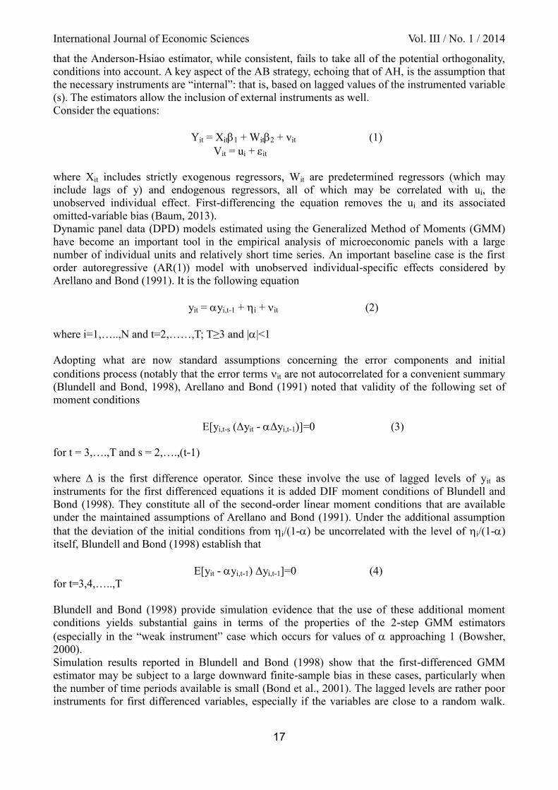
Consider the equations:
Yit = Xit1 + Wit2 + vit (1)
Vit = ui + it
where Xit includes strictly exogenous regressors, Wit are predetermined regressors (which may
include lags of y) and endogenous regressors, all of which may be correlated with ui, the
unobserved individual effect. First-differencing the equation removes the ui and its associated
omitted-variable bias (Baum, 2013).
Dynamic panel data (DPD) models estimated using the Generalized Method of Moments (GMM)
have become an important tool in the empirical analysis of microeconomic panels with a large
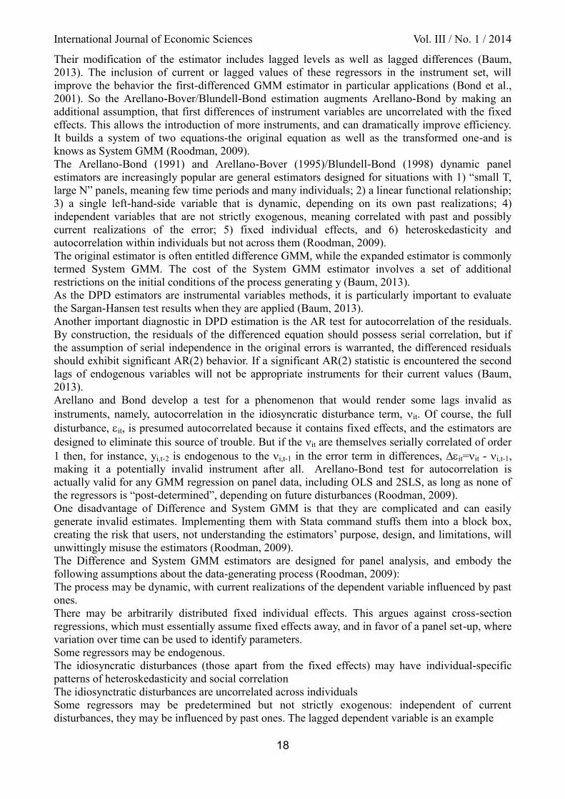
number of individual units and relatively short time series. An important baseline case is the first
order autoregressive (AR(1)) model with unobserved individual-specific effects considered by
Arellano and Bond (1991). It is the following equation
yit = yi,t-1 + i + it (2)
where i=1,…..,N and t=2,……,T; T≥3 and ||<1
Adopting what are now standard assumptions concerning the error components and initial
conditions process (notably that the error terms it are not autocorrelated for a convenient summary
(Blundell and Bond, 1998), Arellano and Bond (1991) noted that validity of the following set of
moment conditions
E[yi,t-s (Δyit - Δyi,t-1)]=0 (3)
for t = 3,….,T and s = 2,….,(t-1)
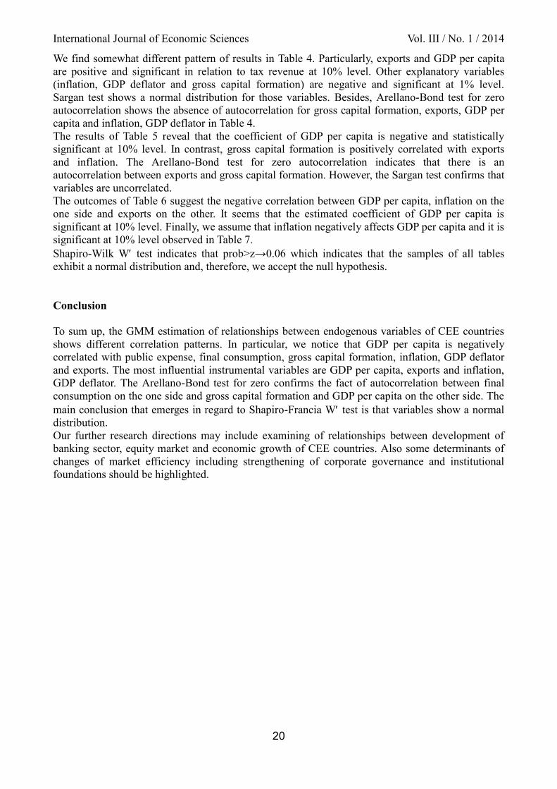
where Δ is the first difference operator. Since these involve the use of lagged levels of yit as
instruments for the first differenced equations it is added DIF moment conditions of Blundell and
Bond (1998). They constitute all of the second-order linear moment conditions that are available
under the maintained assumptions of Arellano and Bond (1991). Under the additional assumption
that the deviation of the initial conditions from i/(1-) be uncorrelated with the level of i/(1-)
itself, Blundell and Bond (1998) establish that
E[yit - yi,t-1) Δyi,t-1]=0 (4)
for t=3,4,…..,T
Blundell and Bond (1998) provide simulation evidence that the use of these additional moment
conditions yields substantial gains in terms of the properties of the 2-step GMM estimators
(especially in the “weak instrument” case which occurs for values of approaching 1 (Bowsher,
2000).
Simulation results reported in Blundell and Bond (1998) show that the first-differenced GMM
estimator may be subject to a large downward finite-sample bias in these cases, particularly when
the number of time periods available is small (Bond et al., 2001). The lagged levels are rather poor
instruments for first differenced variables, especially if the variables are close to a random walk.
International Journal of Economic Sciences Vol. III / No. 1 / 2014
18
Their modification of the estimator includes lagged levels as well as lagged differences (Baum,
2013). The inclusion of current or lagged values of these regressors in the instrument set, will
improve the behavior the first-differenced GMM estimator in particular applications (Bond et al.,
2001). So the Arellano-Bover/Blundell-Bond estimation augments Arellano-Bond by making an
additional assumption, that first differences of instrument variables are uncorrelated with the fixed
effects. This allows the introduction of more instruments, and can dramatically improve efficiency.
It builds a system of two equations-the original equation as well as the transformed one-and is
knows as System GMM (Roodman, 2009).
The Arellano-Bond (1991) and Arellano-Bover (1995)/Blundell-Bond (1998) dynamic panel
estimators are increasingly popular are general estimators designed for situations with 1) “small T,
large N” panels, meaning few time periods and many individuals; 2) a linear functional relationship;
3) a single left-hand-side variable that is dynamic, depending on its own past realizations; 4)
independent variables that are not strictly exogenous, meaning correlated with past and possibly
current realizations of the error; 5) fixed individual effects, and 6) heteroskedasticity and
autocorrelation within individuals but not across them (Roodman, 2009).
The original estimator is often entitled difference GMM, while the expanded estimator is commonly
termed System GMM. The cost of the System GMM estimator involves a set of additional
restrictions on the initial conditions of the process generating y (Baum, 2013).
As the DPD estimators are instrumental variables methods, it is particularly important to evaluate
the Sargan-Hansen test results when they are applied (Baum, 2013).
Another important diagnostic in DPD estimation is the AR test for autocorrelation of the residuals.
By construction, the residuals of the differenced equation should possess serial correlation, but if
the assumption of serial independence in the original errors is warranted, the differenced residuals
should exhibit significant AR(2) behavior. If a significant AR(2) statistic is encountered the second
lags of endogenous variables will not be appropriate instruments for their current values (Baum,
2013).
Arellano and Bond develop a test for a phenomenon that would render some lags invalid as
instruments, namely, autocorrelation in the idiosyncratic disturbance term, it. Of course, the full
disturbance, it, is presumed autocorrelated because it contains fixed effects, and the estimators are
designed to eliminate this source of trouble. But if the it are themselves serially correlated of order
1 then, for instance, yi,t-2 is endogenous to the i,t-1 in the error term in differences, it=it - i,t-1,
making it a potentially invalid instrument after all. Arellano-Bond test for autocorrelation is
actually valid for any GMM regression on panel data, including OLS and 2SLS, as long as none of
the regressors is “post-determined”, depending on future disturbances (Roodman, 2009).
One disadvantage of Difference and System GMM is that they are complicated and can easily
generate invalid estimates. Implementing them with Stata command stuffs them into a block box,
creating the risk that users, not understanding the estimators’ purpose, design, and limitations, will
unwittingly misuse the estimators (Roodman, 2009).
The Difference and System GMM estimators are designed for panel analysis, and embody the
following assumptions about the data-generating process (Roodman, 2009):
The process may be dynamic, with current realizations of the dependent variable influenced by past
ones.
There may be arbitrarily distributed fixed individual effects. This argues against cross-section
regressions, which must essentially assume fixed effects away, and in favor of a panel set-up, where
variation over time can be used to identify parameters.
Some regressors may be endogenous.
The idiosyncratic disturbances (those apart from the fixed effects) may have individual-specific
patterns of heteroskedasticity and social correlation
The idiosynctratic disturbances are uncorrelated across individuals
Some regressors may be predetermined but not strictly exogenous: independent of current
disturbances, they may be influenced by past ones. The lagged dependent variable is an example
International Journal of Economic Sciences Vol. III / No. 1 / 2014
19
The number of time periods of available data, T, may be small
Finally, since the estimators are designed for general use, they do not assume that good instruments
are available outside the immediate data set.
The numerical methods of normality include the Kolmogorov-Smirnov (K-S) test, Lilliefors test,
Shapiro-Wilk test, Anderson-Darling test, and Cramer-von Misestest (SAS Institute 1995). The K-S
test and Shapiro-Wilk W’ test are commonly used. The K-S, Anderson-Darling, and Cramer-von
Misers tests are based on the empirical distribution function (EDF) which is defined as a set of N
independent observations x1,x2,……xn with a common distribution function F(x) (SAS 2004)
(Myoung, 2008).
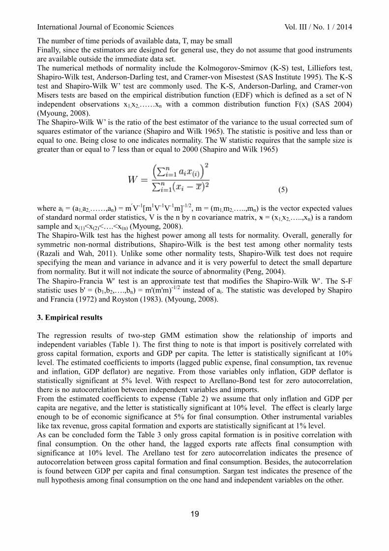
The Shapiro-Wilk W’ is the ratio of the best estimator of the variance to the usual corrected sum of
squares estimator of the variance (Shapiro and Wilk 1965). The statistic is positive and less than or
equal to one. Being close to one indicates normality. The W statistic requires that the sample size is
greater than or equal to 7 less than or equal to 2000 (Shapiro and Wilk 1965)
(5)
where ai = (a1,a2,……,an) = mV
-1[m
1V
-1V
-1m]
-1/2, m = (m1,m2,…..,mn) is the vector expected values
of standard normal order statistics, V is the n by n covariance matrix, x = (x1,x2,…..,xn) is a random
sample and x(1)<x(2)<….<x(n) (Myoung, 2008).
The Shapiro-Wilk test has the highest power among all tests for normality. Overall, generally for
symmetric non-normal distributions, Shapiro-Wilk is the best test among other normality tests
(Razali and Wah, 2011). Unlike some other normality tests, Shapiro-Wilk test does not require
specifying the mean and variance in advance and it is very powerful to detect the small departure
from normality. But it will not indicate the source of abnormality (Peng, 2004).
The Shapiro-Francia W test is an approximate test that modifies the Shapiro-Wilk W. The S-F
statistic uses b' = (b1,b2,….,bn) = m'(m'm)-1/2
instead of ai. The statistic was developed by Shapiro
and Francia (1972) and Royston (1983). (Myoung, 2008).
3. Empirical results
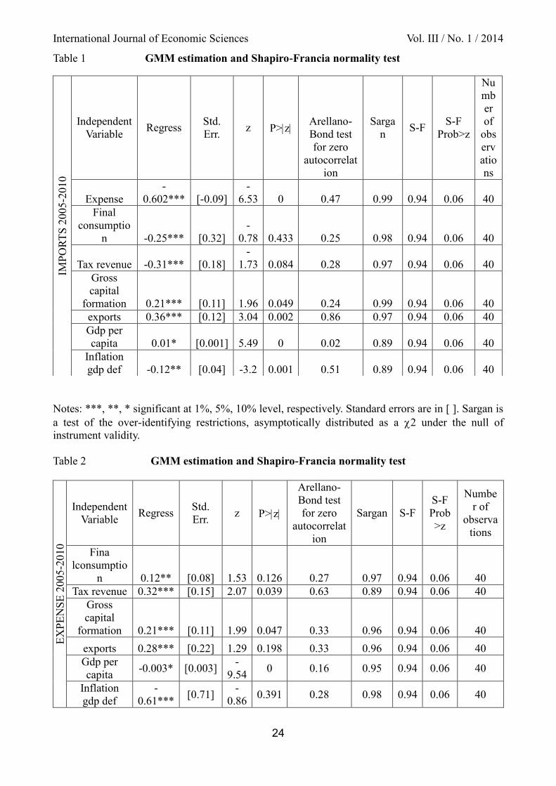
The regression results of two-step GMM estimation show the relationship of imports and
independent variables (Table 1). The first thing to note is that import is positively correlated with
gross capital formation, exports and GDP per capita. The letter is statistically significant at 10%
level. The estimated coefficients to imports (lagged public expense, final consumption, tax revenue
and inflation, GDP deflator) are negative. From those variables only inflation, GDP deflator is
statistically significant at 5% level. With respect to Arellano-Bond test for zero autocorrelation,
there is no autocorrelation between independent variables and imports.
From the estimated coefficients to expense (Table 2) we assume that only inflation and GDP per
capita are negative, and the letter is statistically significant at 10% level. The effect is clearly large
enough to be of economic significance at 5% for final consumption. Other instrumental variables
like tax revenue, gross capital formation and exports are statistically significant at 1% level.
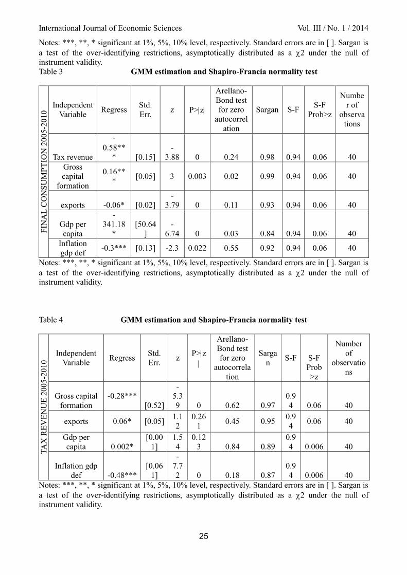
As can be concluded form the Table 3 only gross capital formation is in positive correlation with
final consumption. On the other hand, the lagged exports rate affects final consumption with
significance at 10% level. The Arellano test for zero autocorrelation indicates the presence of
autocorrelation between gross capital formation and final consumption. Besides, the autocorrelation
is found between GDP per capita and final consumption. Sargan test indicates the presence of the
null hypothesis among final consumption on the one hand and independent variables on the other.
International Journal of Economic Sciences Vol. III / No. 1 / 2014
20
We find somewhat different pattern of results in Table 4. Particularly, exports and GDP per capita
are positive and significant in relation to tax revenue at 10% level. Other explanatory variables
(inflation, GDP deflator and gross capital formation) are negative and significant at 1% level.
Sargan test shows a normal distribution for those variables. Besides, Arellano-Bond test for zero
autocorrelation shows the absence of autocorrelation for gross capital formation, exports, GDP per
capita and inflation, GDP deflator in Table 4.
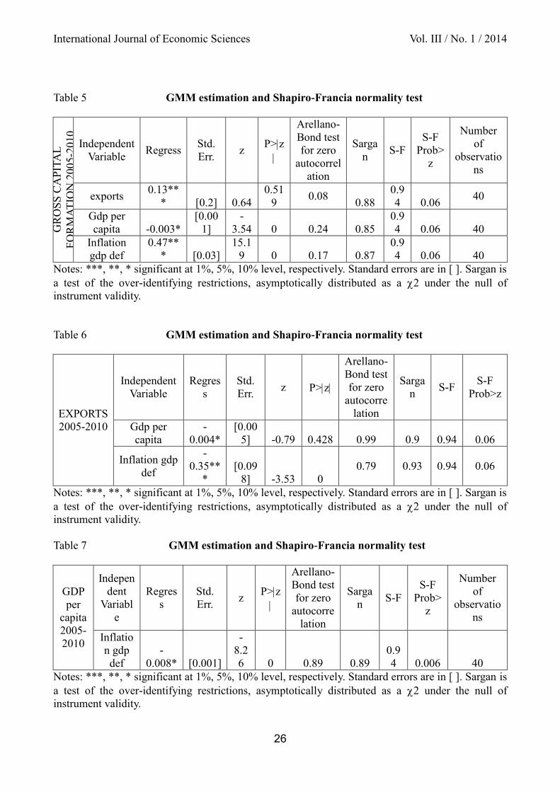
The results of Table 5 reveal that the coefficient of GDP per capita is negative and statistically
significant at 10% level. In contrast, gross capital formation is positively correlated with exports
and inflation. The Arellano-Bond test for zero autocorrelation indicates that there is an
autocorrelation between exports and gross capital formation. However, the Sargan test confirms that
variables are uncorrelated.
The outcomes of Table 6 suggest the negative correlation between GDP per capita, inflation on the
one side and exports on the other. It seems that the estimated coefficient of GDP per capita is
significant at 10% level. Finally, we assume that inflation negatively affects GDP per capita and it is
significant at 10% level observed in Table 7.
Shapiro-Wilk W test indicates that prob>z→0.06 which indicates that the samples of all tables
exhibit a normal distribution and, therefore, we accept the null hypothesis.
Conclusion
To sum up, the GMM estimation of relationships between endogenous variables of CEE countries
shows different correlation patterns. In particular, we notice that GDP per capita is negatively
correlated with public expense, final consumption, gross capital formation, inflation, GDP deflator
and exports. The most influential instrumental variables are GDP per capita, exports and inflation,
GDP deflator. The Arellano-Bond test for zero confirms the fact of autocorrelation between final
consumption on the one side and gross capital formation and GDP per capita on the other side. The
main conclusion that emerges in regard to Shapiro-Francia W test is that variables show a normal
distribution.
Our further research directions may include examining of relationships between development of
banking sector, equity market and economic growth of CEE countries. Also some determinants of
changes of market efficiency including strengthening of corporate governance and institutional
foundations should be highlighted.
International Journal of Economic Sciences Vol. III / No. 1 / 2014
21
References
Abrams B. A., (1999) “The effects of government size on the unemployment rate”, Public Choice
99: 395-401
Agbeyegbe T., Stotshky J. G., WoldeMariam A., (2004) “Trade liberalization, exchange rate
changes, and tax revenue in Sub-Saharan Africa”, IMF Working paper, WP/04/178/, p. 11
Aguirre A., Calderon C., (2006) “The real exchange rate misalignment and economic performance”,
Central Bank of Chile, Working paper no. 315
Alexiou C., (2009) “Government spending and economic growth: Econometric evidence from the
South Eastern Europe (SEE)”, Journal of Economic and Social Research, 11(1), 1-16
Anderson T., W., Hsiao C. (1981) “Estimation of dynamic models with error components”, Journal
of American Statistical Association, 76, 598-606
Arellano M., (1989) “A note on the Anderson-Hsiao estimator for panel data”, Economics Letters,
vol. 31, pp. 337-341
Arellano M., Bond S., (1991) “Some tests of specification for panel data: Monte Carlo evidence and
an application to employment equations”, Review of Economic Studies, 58, 277-297
Arellano M., Honore B., (2001) “Panel data models: Some recent developments”, in E. Leamer and
J. Heckman, eds., Handbook of Econometrics, vol. 5, pp. 3229-3296
Arellano M., Bover O., (1995) “another look at the instrumental variable estimation of error
components models”, Journal of Econometrics 68, pp. 29-51
Aschauer A. D., (1990) “Is government spending stimulative?” Contemporary Policy Issues 8. 30-
45
Asiedu E., (2002) “On the determinants of foreign direct investment to developing countries: Is
Africa different”, World Development, 30(1), 107-119
Asiedu E., (2006) “Foreign direct investment in Africa: The role of natural resources, market size,
government policy, institutions and political instability”, The World Economy, 29(1), 63-77
Ball L., Cechetti S., (1991) “Inflation and uncertainty at short and long horizons”, NBER Reprints
1522
Barro R. J. (1991) “Economic growth in a cross-section of countries”, Quarterly Journal of
Economics 106: 407-43
Baum C. F., (2013) “Dynamic panel data estimators”, Applied Econometrics, EC823, 1-50
Baum C. F., (2013) “Panel data management, estimation and forecasting”, Birmingham Business
School, p. 9
Bleany M., Greenaway D., (2001) “The impact of terms of trade and real exchange rate volatility on
investment and growth in Sub-Saharan Africa”, Journal of Development Economics, 65, 491-500
Blundell R., Bond S., (1998) “Initial conditions and moment restrictions in dynamic panel data
models”, Journal of Econometrics, 87, 115-143
Bond S., (2002) “Dynamic panel data models: A guide to micro data methods and practice”, The
Institute for Fiscal Studies, Department of Economics, UCL, working paper CWP09/02
Bond S., Hoeffler A., Temple J., (2001) “GMM estimation of empirical growth models”, CEPR
Discussion papers 3048, C. E. P. R. Discussion papers
Bowsher C. G., (2002) “On testing over-identifying restrictions in dynamic panel data models”,
Economics Letters, vol.77: 211-220
Carlstrom C., Gokhale J., (1991) “Government consumption, taxation, and economic activity”,
Federal Reserve Bank of Cleveland, Economic Review 3rd
Quarter: 28-45
Cizkowicz P., Rzanka A., (2012) “Does inflation harm corporate investment? Empirical evidence
from OECD countries”, Economics Journal, Discussion paper no. 2012-63, p. 4
Collins M., Ofair R. S., (1997) “Real exchange rate misalignments and growth”, NBER Working
paper
Conte M. A., Darrat A. F., (1988) “Economic growth and the expanding public sector: A re-
examination”, Review of Economics and Statistics 70(2): 322-30
International Journal of Economic Sciences Vol. III / No. 1 / 2014
22
Cottani J., Cavalo D., Khan M. S. (1990) “Real exchange rate behavior and economic performance
in LDCs”, Economic Development and Cultural Change, 39(1), 61-76
Desai M., Hines J. Jr., (1997) “Excess capital flows and the burdens of inflation in open
economics”, NBER Working papers 6064
ECB (2010) “The impact of the financial crisis on the Central and Eastern European countries”,
ECB, Monthly Bulletin, p. 89
Egert B., Drine I., Lommatzsch K., Rault C., (2003) “The Balassa-Samuelson effect in Central and
Eastern Europe: Myth or reality? Journal of Comparative Economics, vol. 31, no. 3: 552-572
Egert B., Lommatzsch K., Lahreche-Revil A., (2006) “Real exchange rates in small open OECD
and transition economies: Comparing apples with oranges?” Journal of Banking and Finance,
vol.30, no.12: 3393-3406
Egert B., Podpiera, J., (2008) “Structural inflation and real exchange rate appreciation in Visegrad-4
countries: Balassa-Samuelson or something else?” CEPR Policy Insight 20,
http://www.cepr.org/pubs/PolicyInsights/PolicyInsight20.pdf
Engen E., Skinner J. (1992) “Fiscal policy and economic growth”, National Bureau of Economic
Research, Working paper no. 4223
Evans M., (1991) “Discovering the link between inflation rates and inflation uncertainty”, Journal
of Money, Credit and Banking 23(2): 169-84
Evans M., Wachtel P., (1993) “Inflation regimes and the sources of inflation uncertainty”, Federal
Reserve Bank of Cleveland Proceedings: 475-520
Fabrizio S., Igan D., Mody A., (2007) “The dynamics of product quality and international
competitiveness”, IMF Working paper, No. WP/07/97
Feldstein M., Green J. R., Sheshinski E., (1978) “Inflation and taxes in a growing economy with
debt and equity finance”, Journal of Political Economy 86(2): 53-70
Ferderer J. P., (1993) “The impact of uncertainty on aggregate investment spending: An empirical
analysis”, Journal of Money, Credit and Banking 25(1): 30-48
Fisher G., (2009) “Investment choice and inflation uncertainty”, London School of Economics,
nimeo
Ghali K. H., (1998) “Government size and economic growth: Evidence from a multivariate
analysis”, Applied Economics 31: 975-987
Ghura D., (1998) “Tax revenue in Sub-Saharan Africa: Effects of economic policies and
corruption”, IMF working paper 98/135, Washington: International Monetary Fund
Gillman M., Nakov A., (2004) “Granger causality of the inflation-growth, mirror in accession
countries”, Economics of Transition 12, 4: 653-681
Guseh J. S., (1997) “Government size and economic growth in developing countries: A political-
economy framework”, Journal of Macroeconomics 19(1): 175-192
Han C., Phillips P. C. B., (2010) “GMM estimation for dynamics panels with fixed effects and
strong instruments at unity”, Econometric Theory, Cambridge University Press, 26, 119-151
Hartman R., (1980) “Taxation and the effects of inflation on the real capital stock in an open
economy”, NBER Reprints 0117
Hasanov M., Omay T., (2010) “The relationship between inflation, output growth, and their
uncertainties: Evidence from selected CEE countries”, MPRA paper no. 23764, p. 2
Jenkins C., Thomas L., (2002) “Foreign direct investment in Southern Africa: determinants,
characteristics and implications for economic growth and poverty alleviation”, University of
Oxford. Available online at http://www.csae.ox.ac.uk/reports/pdfs/rep2002-02.pdf
Jong-Wha L., (1995) “Capital goods imports and long-run growth”, Journal of Development
Economics, 48(1): 91-110
Kalckreuth von U., (2000) “Exploring the role uncertainty for corporate investment decisions in
Germany”, Deutsche Bundesbank Research Centre Discussion paper series. Economic Studies 05
Khan S., Senhadji A., Smith B. D., (2006) “Inflation and financial depth”, Macroeconomic
Dynamics 10(02): 165-182
International Journal of Economic Sciences Vol. III / No. 1 / 2014
23
Kolluri B. R., Panik M. J., Wahab M. S., (2000) “Government expenditure and economic growth:
Evidence from G7 countries”, Applied Economics 32: 1059-1068
Liam E., Stotsky J., Grapp R., (1999) “Revenue implications of trade liberalization”, IMF
Occasional paper 99/80, Washington: International Monetary Fund
Loizidis J., Vamvoukas G., (2004) “Government expenditure and economic growth: Evidence from
trivariate causality testing”, Journal of Applied Economics, vol. 8, no. 1, 125-152
Markusen J. R., Venables A. J., (1995) “Multinational firms and the new trade theory” NBER
Working paper, No. 5036, Cambridge Mass
Mundell R., (1957) “International trade and factor mobility”, American Economic Review, 47(3),
321-335
Myoung H. P., (2008) “Univariate analysis and normality test using SAS, Stata, and SPSS”, The
University Information Technology Services (UITS) Center for Statistical and Mathematical
Computing, Indiana University, Tech. Rep., 2008, available at http://www.indiana.edu/stat-
math/stat/all/normality/normality.pdf
Nickell S., (1981)”Baises in dynamic models with fixed effects”, Econometrica, 49, 1417-1426
Peng G., (2004) “Testing normality of data using SAS”, Eli Lilly and Company, PO04, p. 1
Razali N. M., Wah Y. B., (2011) “Power comparisons of Shapiro-Wilk, Kolmogorov-Smirnov,
Lilliefers and Anderson-Darling tests”, Journal of Statistical Modeling and Analysis, vol. 2 no. 1,
21-33
Rodrick D., (2007) “The real exchange rate and economic growth: Theory and evidence”, John F.
Kennedy School of Government, Harvard University
Roodman D., (2009) “How to do xtabond2: an introduction to difference and system GMM in Stata,
The Stata Journal, no. 1, pp. 86-136
Royston J. P., (1983) “A simple method for evaluating the Shapiro-Francia W test of non-
normality”, Statistician, 32(3): 297-300
Shapiro S. S., Francia R. S., (1972) “An approximate analysis of variance test for normality”,
Journal of the American Statistical Assocation, 67 (337): 215-216
Shapiro S. S., Wilk M. B., (1965) “An analysis of variance test for normality (Complete Samples)”,
Biometrica, 52 (3/4): 591-611
Singh B., Sahni B. S., (1984)”Causality between public expenditure and national income”, The
Review of Economics and Statistics 66: 630-44
Staehr K., (2010) “Inflation in the new EU countries from Central and Eastern Europe: Theories
and panel data estimations”, Bank of Estonia, working paper series 6/2010, p. 13
Tanzi V., (1987) “Quantitative characteristics of the tax systems of developing countries in the
theory of taxation for developing countries”, ed. by David Newberry and Nicholas Stern, New York
and Oxford: Oxford University Press, published for the World Bank, pp. 205-41
Thornton J., (2007) “The relationship between inflation and inflation uncertainty in emerging
market economics”, Southern Economic Journal 73, 4: 858-870
Turkan K., (2006) “Foreign outward direct investment and intermediate goods exports: Evidence
from USA”, paper presented on the ETSG 2006,
http://www.etsg.org/ETSG2006/papers/Turkcan.pdf.
Weinhold D., (1999) “A dynamic “Fixed effects” model for heterogenous panel data”, London
School of Economics, p. 3
Willamson O., (1975) “Markets and hierarchies: Analysis and antitrust implications”, Free Press:
New York
Windmeijer F., (2000) “A finite sample correction for the variance of linear two-step GMM
estimators”, Institute for Fiscal Studies Working paper series no. W00/19
International Journal of Economic Sciences Vol. III / No. 1 / 2014
24
Table 1 GMM estimation and Shapiro-Francia normality test
Notes: ***, **, * significant at 1%, 5%, 10% level, respectively. Standard errors are in [ ]. Sargan is
a test of the over-identifying restrictions, asymptotically distributed as a 2 under the null of
instrument validity.
Table 2 GMM estimation and Shapiro-Francia normality test
EX
PE
NS
E 2
005
-2010
Independent
Variable Regress
Std.
Err. z P>z
Arellano-
Bond test
for zero
autocorrelat
ion
Sargan S-F
S-F
Prob
>z
Numbe
r of
observa
tions
Fina
lconsumptio
n 0.12** [0.08] 1.53 0.126 0.27 0.97 0.94 0.06 40
Tax revenue 0.32*** [0.15] 2.07 0.039 0.63 0.89 0.94 0.06 40
Gross
capital
formation 0.21*** [0.11] 1.99 0.047 0.33 0.96 0.94 0.06 40
exports 0.28*** [0.22] 1.29 0.198 0.33 0.96 0.94 0.06 40
Gdp per
capita -0.003* [0.003]
-
9.54 0 0.16 0.95 0.94 0.06 40
Inflation
gdp def
-
0.61*** [0.71]
-
0.86 0.391 0.28 0.98 0.94 0.06 40
IMP
OR
TS
20
05-2
010
Independent
Variable Regress
Std.
Err. z P>z
Arellano-
Bond test
for zero
autocorrelat
ion
Sarga
n S-F
S-F
Prob>z
Nu
mb
er
of
obs
erv
atio
ns
Expense
-
0.602*** [-0.09]
-
6.53 0 0.47 0.99 0.94 0.06 40
Final
consumptio
n -0.25*** [0.32]
-
0.78 0.433 0.25 0.98 0.94 0.06 40
Tax revenue -0.31*** [0.18]
-
1.73 0.084 0.28 0.97 0.94 0.06 40
Gross
capital
formation 0.21*** [0.11] 1.96 0.049 0.24 0.99 0.94 0.06 40
exports 0.36*** [0.12] 3.04 0.002 0.86 0.97 0.94 0.06 40
Gdp per
capita 0.01* [0.001] 5.49 0 0.02 0.89 0.94 0.06 40
Inflation
gdp def -0.12** [0.04] -3.2 0.001 0.51 0.89 0.94 0.06 40
International Journal of Economic Sciences Vol. III / No. 1 / 2014
25
Notes: ***, **, * significant at 1%, 5%, 10% level, respectively. Standard errors are in [ ]. Sargan is
a test of the over-identifying restrictions, asymptotically distributed as a 2 under the null of
instrument validity.
Table 3 GMM estimation and Shapiro-Francia normality test
FIN
AL
CO
NS
UM
PT
ION
2005
-2010 Independent
Variable Regress
Std.
Err. z P>z
Arellano-
Bond test
for zero
autocorrel
ation
Sargan S-F S-F
Prob>z
Numbe
r of
observa
tions
Tax revenue
-
0.58**
* [0.15]
-
3.88 0 0.24 0.98 0.94 0.06 40
Gross
capital
formation
0.16**
* [0.05] 3 0.003 0.02 0.99 0.94 0.06 40
exports -0.06* [0.02]
-
3.79 0 0.11 0.93 0.94 0.06 40
Gdp per
capita
-
341.18
*
[50.64
]
-
6.74 0 0.03 0.84 0.94 0.06 40
Inflation
gdp def -0.3*** [0.13] -2.3 0.022 0.55 0.92 0.94 0.06 40
Notes: ***, **, * significant at 1%, 5%, 10% level, respectively. Standard errors are in [ ]. Sargan is
a test of the over-identifying restrictions, asymptotically distributed as a 2 under the null of
instrument validity.
Table 4 GMM estimation and Shapiro-Francia normality test
TA
X R
EV
EN
UE
2005
-2010
Independent
Variable Regress
Std.
Err. z
P>z
Arellano-
Bond test
for zero
autocorrela
tion
Sarga
n S-F S-F
Prob
>z
Number
of
observatio
ns
Gross capital
formation
-0.28***
[0.52]
-
5.3
9 0 0.62 0.97
0.9
4 0.06 40
exports 0.06* [0.05] 1.1
2
0.26
1 0.45 0.95
0.9
4 0.06 40
Gdp per
capita 0.002*
[0.00
1]
1.5
4
0.12
3 0.84 0.89
0.9
4 0.006 40
Inflation gdp
def -0.48***
[0.06
1]
-
7.7
2 0 0.18 0.87
0.9
4 0.006 40
Notes: ***, **, * significant at 1%, 5%, 10% level, respectively. Standard errors are in [ ]. Sargan is
a test of the over-identifying restrictions, asymptotically distributed as a 2 under the null of
instrument validity.
International Journal of Economic Sciences Vol. III / No. 1 / 2014
26
Table 5 GMM estimation and Shapiro-Francia normality test
GR
OS
S C
AP
ITA
L
FO
RM
AT
ION
2005
-2010
Independent
Variable Regress
Std.
Err. z
P>z
Arellano-
Bond test
for zero
autocorrel
ation
Sarga
n S-F
S-F
Prob>
z
Number
of
observatio
ns
exports 0.13**
* [0.2] 0.64
0.51
9 0.08
0.88
0.9
4 0.06 40
Gdp per
capita -0.003*
[0.00
1]
-
3.54 0 0.24 0.85
0.9
4 0.06 40
Inflation
gdp def
0.47**
* [0.03]
15.1
9 0 0.17 0.87
0.9
4 0.06 40
Notes: ***, **, * significant at 1%, 5%, 10% level, respectively. Standard errors are in [ ]. Sargan is
a test of the over-identifying restrictions, asymptotically distributed as a 2 under the null of
instrument validity.
Table 6 GMM estimation and Shapiro-Francia normality test
EXPORTS
2005-2010
Independent
Variable
Regres
s
Std.
Err. z P>z
Arellano-
Bond test
for zero
autocorre
lation
Sarga
n S-F
S-F
Prob>z
Gdp per
capita
-
0.004*
[0.00
5] -0.79 0.428 0.99 0.9 0.94 0.06
Inflation gdp
def
-
0.35**
*
[0.09
8] -3.53 0
0.79 0.93 0.94 0.06
Notes: ***, **, * significant at 1%, 5%, 10% level, respectively. Standard errors are in [ ]. Sargan is
a test of the over-identifying restrictions, asymptotically distributed as a 2 under the null of
instrument validity.
Table 7 GMM estimation and Shapiro-Francia normality test
GDP
per
capita
2005-
2010
Indepen
dent
Variabl
e
Regres
s
Std.
Err. z
P>z
Arellano-
Bond test
for zero
autocorre
lation
Sarga
n S-F
S-F
Prob>
z
Number
of
observatio
ns
Inflatio
n gdp
def
-
0.008* [0.001]
-
8.2
6 0 0.89 0.89
0.9
4 0.006 40
Notes: ***, **, * significant at 1%, 5%, 10% level, respectively. Standard errors are in [ ]. Sargan is
a test of the over-identifying restrictions, asymptotically distributed as a 2 under the null of
instrument validity.