PONTIFICAL CATHOLIC UNIVERSITY OF RIO GRANDE DO SULFACULTY OF INFORMATICS

COMPUTER SCIENCE GRADUATE PROGRAM

GMAVIS: A DOMAIN-SPECIFICLANGUAGE FOR

LARGE-SCALE GEOSPATIALDATA VISUALIZATION

SUPPORTING MULTI-COREPARALLELISM

CLEVERSON LOPES LEDUR

Thesis submitted to the Pontifical CatholicUniversity of Rio Grande do Sul in partialfullfillment of the requirements for thedegree of Master in Computer Science.

Advisor: Prof. Ph.D. Luiz Gustavo Leão FernandesCo-Advisor: Prof. Ph.D. Isabel Harb Manssour

Porto Alegre2016

Dados Internacionais de Catalogação na Publicação (CIP)

L475g Ledur, Cleverson Lopes

Gmavis : a domain-specific language for large-scale geospatial

data visualization supporting multi-core parallelism / Cleverson

Lopes Ledur. – 2016.

143 p.

Diss. (Mestrado) – Faculdade de Informática, Pontifícia

Universidade Católica do Rio Grande do Sul.

Orientador: Prof. Dr. Luiz Gustavo Leão Fernandes

Co-Orientador: Prof. Dr. Isabel Harb Manssour

1. Linguagem de Programação de Domínio Específico

(Computadores). 2. Processamento Paralelo (Computadores).

3. Dados Geoespaciais. 4. Visualização de Informação.

5. Informática. I. Fernandes, Luiz Gustavo Leão. II. Manssour,

Isabel Harb. III. Título.

CDD 23 ed. 005.133

Salete Maria Sartori CRB 10/1363

Setor de Tratamento da Informação da BC-PUCRS

This thesis is dedicated to my parents for their endless love, support and encour-agement, and to all the people who never stop believing in me.

“I found I could say things with color and shapesthat I couldn’t say any other way, things I hadno words for.”(Georgia O’Keeffe)

ACKNOWLEDGMENTS

First, I would like to thank my advisors for guiding this research and helping duringthe hard times. Also, I thank my colleague Dalvan Griebler who provided insight and ex-pertise that greatly assisted in the research. I would like to thank the research support ofFAPERGS (Fundação de Amparo à Pesquisa do Estado do Rio Grande do Sul) and CAPES(Coordenação de Aperfeiçoamento Pessoal de Nível Superior). Additionally, I would like tothank the financial support of FACIN (Faculdade de Informática) and PPGCC (Programa dePós-Graduação em Ciência da Computação). Personally, I would like to thank my parentsand my brother to the support and patience during the hard work. Also, I want to especiallythank my aunts Letícia and Varlenes who gave me my first computer when I was a child andprovided support in many moments of my life.

GMAVIS: UMA LINGUAGEM ESPECÍFICA DE DOMÍNIO PARAVISUALIZAÇÕES DE DADOS GEOESPACIAIS EM LARGA ESCALA

COM SUPORTE A PARALELISMO EM ARQUITETURAS MULTI-CORE

RESUMO

A geração de dados tem aumentado exponencialmente nos últimos anos devidoà popularização da tecnologia. Ao mesmo tempo, a visualização da informações permitea extração de conhecimentos e informações úteis através de representação de dados comelementos gráficos. Diferentes técnicas de visualização auxiliam na percepção de infor-mações sobre os dados, tal como a identificação de padrões ou anomalias. Apesar dosbenefícios, muitas vezes a geração de uma visualização pode ser uma tarefa difícil paraos usuários com baixo conhecimento em programação de computadores. E torna-se maisdifícil quando esses usuários precisam lidar com grandes arquivos de dados, uma vez quea maioria das ferramentas não oferece os recursos para abstrair o pré-processamento dedados. Considerando este contexto, neste trabalho é proposta e descrita a GMaVis, umalinguagem específica de domínio (DSL), que permite uma descrição de alto nível para a cria-ção de visualizações usando dados geoespaciais através de um pré-processador de dadosparalelo e um gerador de visualizações. GMaVis foi avaliada utilizando duas abordagens.Na primeira foi realizada uma análise de esforço de programação, através de um softwarepara estimar o esforço de desenvolvimento com base no código. Esta avaliação demons-trou um alto ganho em produtividade quando comparado com o esforço de programaçãoexigido com APIs ou bibliotecas que possuem a mesma finalidade. Na segunda abordagemfoi realizada uma avaliação de desempenho no pré-processador de dados paralelo, quedemonstrou um ganho de desempenho quando comparado com a versão sequencial.

Palavras-Chave: DSL, Visualização de Informações, Dados Geoespaciais, ProcessamentoParalelo de Dados.

GMAVIS: A DOMAIN-SPECIFIC LANGUAGE FOR LARGE-SCALEGEOSPATIAL DATA VISUALIZATION SUPPORTING MULTI-CORE

PARALLELISM

ABSTRACT

Data generation has increased exponentially in recent years due to the popular-ization of technology. At the same time, information visualization enables the extraction ofknowledge and useful information through data representation with graphic elements. More-over, a set of visualization techniques may help in information perception, enabling findingpatterns and anomalies in data. Even tought it provides many benefits, the information visu-alization creation is a hard task for users with a low knowledge in computer programming.It becomes more difficult when these users have to deal with big data files since most toolsdo not provide features to abstract data preprocessing. In order to bridge this gap, we pro-posed GMaVis. It is a Domain-Specific Language (DSL) that offers a high-level descriptionlanguage for creating geospatial data visualizations through a parallel data preprocessorand a high-level description language. GMaVis was evaluated using two approaches. Firstwe performed a programming effort analysis, using an analytical software to estimate devel-opment effort based on the code. This evaluation demonstrates a high gain in productivitywhen compared with programming effort required by other tools and libraries with similarpurposes. Also, a performance evaluation was conducted in the parallel module that per-forms data preprocessing, which demonstrated a performance gain when compared with thesequential version.

Keywords: DSL, Information Visualization, Geospatial Data, Parallel Data Processing.

LIST OF FIGURES

Figure 1.1 – Research scenario framework (Extracted from [Gri16]). . . . . . . . . . . . 29

Figure 1.2 – Example of GMaVis code to generate a heatmap. . . . . . . . . . . . . . . . 30

Figure 1.3 – Example of GMaVis code to generate a markedmap. . . . . . . . . . . . . . 31

Figure 2.1 – DSL concepts (Adapted from [VBD+13]). . . . . . . . . . . . . . . . . . . . . . . 36

Figure 2.2 – DSL design steps (Adapted from [MHS05]). . . . . . . . . . . . . . . . . . . . . 38

Figure 2.3 – Data visualization pipeline (Adapted from [CMS99]). . . . . . . . . . . . . . 39

Figure 2.4 – Parallel architectures types (Adapted from [Bar15]). . . . . . . . . . . . . . . 44

Figure 2.5 – Shared memory model (Adapted from [Bar15]). . . . . . . . . . . . . . . . . . 46

Figure 2.6 – Message passing model (Adapted from [Bar15]). . . . . . . . . . . . . . . . . 46

Figure 2.7 – Hybrid model (Adapted from [Bar15]). . . . . . . . . . . . . . . . . . . . . . . . . . 47

Figure 2.8 – Flex workflow (Extracted from [Gao15b]). . . . . . . . . . . . . . . . . . . . . . . 52

Figure 2.9 – Bison workflow (Extracted from [Gao15a]). . . . . . . . . . . . . . . . . . . . . . 53

Figure 3.1 – Vivaldi system overview (Extracted from [CCQ+er]). . . . . . . . . . . . . . . 56

Figure 3.2 – Vivaldi code and output (Extracted from [CCQ+er]). . . . . . . . . . . . . . . 57

Figure 3.3 – Slangs in ViSlang (Extracted from [RBGH14]). . . . . . . . . . . . . . . . . . . 57

Figure 3.4 – Diderot code example using tensors (Extracted from [CKR+12]). . . . . 59

Figure 3.5 – Shadie example (Extracted from [HWCP15]). . . . . . . . . . . . . . . . . . . . 60

Figure 3.6 – Shadie compilation workflow (Extracted from [HWCP15]). . . . . . . . . . 60

Figure 3.7 – Superconductor: design axes for visualization languages (Extractedfrom [MTAB15]). . . . . . . . . . . . . . . . . . . . . . . . . . . . . . . . . . . . . . . . . . . . . . . . 61

Figure 3.8 – Superconductor architecture (Extracted from [MTAB15]). . . . . . . . . . . 62

Figure 3.9 – Code generation in Superconductor (Extracted from [MTAB15]). . . . . 62

Figure 4.1 – Data visualization creation comparison. . . . . . . . . . . . . . . . . . . . . . . . 66

Figure 4.2 – DSL enviroment. . . . . . . . . . . . . . . . . . . . . . . . . . . . . . . . . . . . . . . . . . 67

Figure 4.3 – Logical operators to filter and classify. . . . . . . . . . . . . . . . . . . . . . . . . . 71

Figure 4.4 – Field value in dataset. . . . . . . . . . . . . . . . . . . . . . . . . . . . . . . . . . . . . . 72

Figure 4.5 – GMaVis interface elements. . . . . . . . . . . . . . . . . . . . . . . . . . . . . . . . . 73

Figure 4.6 – GMaVis settings block example. . . . . . . . . . . . . . . . . . . . . . . . . . . . . . 76

Figure 4.7 – Data preprocessor workflow. . . . . . . . . . . . . . . . . . . . . . . . . . . . . . . . . 78

Figure 4.8 – Airports in world (clustered map). . . . . . . . . . . . . . . . . . . . . . . . . . . . . 83

Figure 4.9 – Flickr photos with "Computer" word as tag (clustered map). . . . . . . . . 84

Figure 4.10 – Airports in world (heatmap). . . . . . . . . . . . . . . . . . . . . . . . . . . . . . . . . 85

Figure 4.11 – Traffic accidents in Porto Alegre, Brazil (heatmap). . . . . . . . . . . . . . . . 86

Figure 4.12 – Traffic accidents in Porto Alegre, Brazil (classified marked map). . . . . 87

Figure 4.13 – Flickr photos taken in 2014 classified by used camera brand. . . . . . . 88

Figure 5.1 – GMaVis compiler structure. . . . . . . . . . . . . . . . . . . . . . . . . . . . . . . . . . 89

Figure 5.2 – Example of logical expression transformation. . . . . . . . . . . . . . . . . . . 95

Figure 5.3 – Error example for a syntax error. . . . . . . . . . . . . . . . . . . . . . . . . . . . . . 96

Figure 5.4 – Data preprocessor generation. . . . . . . . . . . . . . . . . . . . . . . . . . . . . . . 99

Figure 5.5 – Example of sequential processing in data preprocessor. . . . . . . . . . . 101

Figure 5.6 – Parallel preprocessor using pipeline strategy. . . . . . . . . . . . . . . . . . . . 101

Figure 5.7 – Illustration of process function code with SPar annotations. . . . . . . . . 102

Figure 5.8 – Illustration of sequential process function code. . . . . . . . . . . . . . . . . . 102

Figure 5.9 – Data visualization generation. . . . . . . . . . . . . . . . . . . . . . . . . . . . . . . . 104

Figure 6.1 – Code productivity results for heatmap applications. . . . . . . . . . . . . . . 113

Figure 6.2 – Code productivity results for clustered map applications. . . . . . . . . . . 113

Figure 6.3 – Code productivity results for marked map applications. . . . . . . . . . . . 114

Figure 6.4 – Cost estimation results for each application. . . . . . . . . . . . . . . . . . . . . 115

Figure 6.5 – Comparison of SPar and TBB for parallelize data preprocessor. . . . . 117

Figure 6.6 – Airports in world (clustered map). . . . . . . . . . . . . . . . . . . . . . . . . . . . . 118

Figure 6.7 – Flickr photos with "computer" word as tag (clustered map). . . . . . . . . 119

Figure 6.8 – Airports in world (heatmap). . . . . . . . . . . . . . . . . . . . . . . . . . . . . . . . . 120

Figure 6.9 – Traffic accidents in Porto Alegre, Brazil (heatmap). . . . . . . . . . . . . . . . 121

Figure 6.10 – Traffic accidents in Porto Alegre, Brazil with classification (markedmap). . . . . . . . . . . . . . . . . . . . . . . . . . . . . . . . . . . . . . . . . . . . . . . . . . . . . . . . 122

Figure 6.11 – Flickr photos classified by camera brand (marked map). . . . . . . . . . . 123

LIST OF TABLES

Table 2.1 – Comparison of parallel programming interfaces. . . . . . . . . . . . . . . . . . . 51

Table 3.1 – Domain of each DSL. . . . . . . . . . . . . . . . . . . . . . . . . . . . . . . . . . . . . . . 63

Table 3.2 – Complexities abstraction in each visualization creation phase. . . . . . . 63

Table 3.3 – Parallel processing in each visualization creation phase. . . . . . . . . . . . 64

Table 4.1 – GMaVis block reserved words. . . . . . . . . . . . . . . . . . . . . . . . . . . . . . . . 69

Table 4.2 – GMaVis properties reserved words. . . . . . . . . . . . . . . . . . . . . . . . . . . . 69

Table 4.3 – GMaVis value reserved words. . . . . . . . . . . . . . . . . . . . . . . . . . . . . . . . 69

Table 4.4 – GMaVis operator reserved words. . . . . . . . . . . . . . . . . . . . . . . . . . . . . 69

Table 4.5 – GMaVis visualization type reserved words. . . . . . . . . . . . . . . . . . . . . . 70

Table 4.6 – Time complexity of search algorithms. . . . . . . . . . . . . . . . . . . . . . . . . . 79

Table 4.7 – Search algorithm comparison considering sorting. . . . . . . . . . . . . . . . . 80

Table 5.1 – Data preprocessor functions for each logical operator. . . . . . . . . . . . . . 95

Table 6.1 – Dataset sizes. . . . . . . . . . . . . . . . . . . . . . . . . . . . . . . . . . . . . . . . . . . . . 106

Table 6.2 – Software category in COCOMO model (Adapted from [Whe16]). . . . . 108

Table 6.3 – COCOMO cost drivers (Adapted from [Whe16]). . . . . . . . . . . . . . . . . . 108

Table 6.4 – Effort estimation in COCOMO model variables (Extracted from [Whe16]).110

Table 6.5 – SLOCCount estimation about cost to develop each application. . . . . . 114

Table 6.6 – SLOC (Physical Lines of Code) for each application. . . . . . . . . . . . . . . 115

Table 6.7 – Completion times (seconds) (Extracted from [LGMF15]). . . . . . . . . . . . 116

Table 6.8 – Lines of code to parallelize data preprocessor using SPar and TBB. . . 117

Table A.1 – MM_DEV - performance results . . . . . . . . . . . . . . . . . . . . . . . . . . . . . . 135

Table A.2 – MM_ACID - performance results . . . . . . . . . . . . . . . . . . . . . . . . . . . . . . 136

Table A.3 – HM_AIR - performance results . . . . . . . . . . . . . . . . . . . . . . . . . . . . . . . 137

Table A.4 – HM_AC - performance results . . . . . . . . . . . . . . . . . . . . . . . . . . . . . . . . 138

Table A.5 – CM_CP - performance results . . . . . . . . . . . . . . . . . . . . . . . . . . . . . . . . 139

Table A.6 – CM_AIR - performance results . . . . . . . . . . . . . . . . . . . . . . . . . . . . . . . 140

LIST OF ACRONYMS

API – Application Programming Interface

AST – Abstract Syntax Tree

BS – Binary Search

CPU – Central Processing Unit

CSS – Cascading Style Sheets

CSV – Comma-Separated Values

CUDA – Compute Unified Device Architecture

D3 – Data-Driven Documents

DSL – Domain-Specific Language

EAF – Effort Adjustment Factor

EBNF – Extended Backus–Naur Form

GPL – General-Purpose Language

GPU – Graphics Processing Unit

HTML – HyperText Markup Language

I/O – Input/Output

IDE – Integrated Development Environment

IS – Interpolation Search

LALR – Look-Ahead Left Right

LS – Linear Search

MATLAB – MATrix LABoratory

MPI – Message Passing Interface

POSIX – Portable Operating System Interface

RAM – Random Access Memory

TBB – Threading Building Blocks

WMS – Warehouse Management System

YACC – Yet Another Compiler Compiler

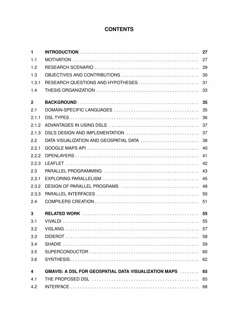
CONTENTS

1 INTRODUCTION . . . . . . . . . . . . . . . . . . . . . . . . . . . . . . . . . . . . . . . . . . . . . . . . . 27

1.1 MOTIVATION . . . . . . . . . . . . . . . . . . . . . . . . . . . . . . . . . . . . . . . . . . . . . . . . . . . . 27

1.2 RESEARCH SCENARIO . . . . . . . . . . . . . . . . . . . . . . . . . . . . . . . . . . . . . . . . . . . 29

1.3 OBJECTIVES AND CONTRIBUTIONS . . . . . . . . . . . . . . . . . . . . . . . . . . . . . . . . 30

1.3.1 RESEARCH QUESTIONS AND HYPOTHESES . . . . . . . . . . . . . . . . . . . . . . . . . 31

1.4 THESIS ORGANIZATION . . . . . . . . . . . . . . . . . . . . . . . . . . . . . . . . . . . . . . . . . . 33

2 BACKGROUND . . . . . . . . . . . . . . . . . . . . . . . . . . . . . . . . . . . . . . . . . . . . . . . . . . 35

2.1 DOMAIN-SPECIFIC LANGUAGES . . . . . . . . . . . . . . . . . . . . . . . . . . . . . . . . . . . 35

2.1.1 DSL TYPES . . . . . . . . . . . . . . . . . . . . . . . . . . . . . . . . . . . . . . . . . . . . . . . . . . . . . 36

2.1.2 ADVANTAGES IN USING DSLS . . . . . . . . . . . . . . . . . . . . . . . . . . . . . . . . . . . . . 37

2.1.3 DSL’S DESIGN AND IMPLEMENTATION . . . . . . . . . . . . . . . . . . . . . . . . . . . . . . 37

2.2 DATA VISUALIZATION AND GEOSPATIAL DATA . . . . . . . . . . . . . . . . . . . . . . . . 38

2.2.1 GOOGLE MAPS API . . . . . . . . . . . . . . . . . . . . . . . . . . . . . . . . . . . . . . . . . . . . . . 40

2.2.2 OPENLAYERS . . . . . . . . . . . . . . . . . . . . . . . . . . . . . . . . . . . . . . . . . . . . . . . . . . . 41

2.2.3 LEAFLET . . . . . . . . . . . . . . . . . . . . . . . . . . . . . . . . . . . . . . . . . . . . . . . . . . . . . . . 42

2.3 PARALLEL PROGRAMMING . . . . . . . . . . . . . . . . . . . . . . . . . . . . . . . . . . . . . . . 43

2.3.1 EXPLORING PARALLELISM . . . . . . . . . . . . . . . . . . . . . . . . . . . . . . . . . . . . . . . . 45

2.3.2 DESIGN OF PARALLEL PROGRAMS . . . . . . . . . . . . . . . . . . . . . . . . . . . . . . . . 48

2.3.3 PARALLEL INTERFACES . . . . . . . . . . . . . . . . . . . . . . . . . . . . . . . . . . . . . . . . . . 50

2.4 COMPILERS CREATION . . . . . . . . . . . . . . . . . . . . . . . . . . . . . . . . . . . . . . . . . . . 51

3 RELATED WORK . . . . . . . . . . . . . . . . . . . . . . . . . . . . . . . . . . . . . . . . . . . . . . . . 55

3.1 VIVALDI . . . . . . . . . . . . . . . . . . . . . . . . . . . . . . . . . . . . . . . . . . . . . . . . . . . . . . . . 55

3.2 VISLANG . . . . . . . . . . . . . . . . . . . . . . . . . . . . . . . . . . . . . . . . . . . . . . . . . . . . . . . 57

3.3 DIDEROT . . . . . . . . . . . . . . . . . . . . . . . . . . . . . . . . . . . . . . . . . . . . . . . . . . . . . . . 58

3.4 SHADIE . . . . . . . . . . . . . . . . . . . . . . . . . . . . . . . . . . . . . . . . . . . . . . . . . . . . . . . . 59

3.5 SUPERCONDUCTOR . . . . . . . . . . . . . . . . . . . . . . . . . . . . . . . . . . . . . . . . . . . . . 60

3.6 SYNTHESIS . . . . . . . . . . . . . . . . . . . . . . . . . . . . . . . . . . . . . . . . . . . . . . . . . . . . . 62

4 GMAVIS: A DSL FOR GEOSPATIAL DATA VISUALIZATION MAPS . . . . . . . . 65

4.1 THE PROPOSED DSL . . . . . . . . . . . . . . . . . . . . . . . . . . . . . . . . . . . . . . . . . . . . 65

4.2 INTERFACE . . . . . . . . . . . . . . . . . . . . . . . . . . . . . . . . . . . . . . . . . . . . . . . . . . . . . 68

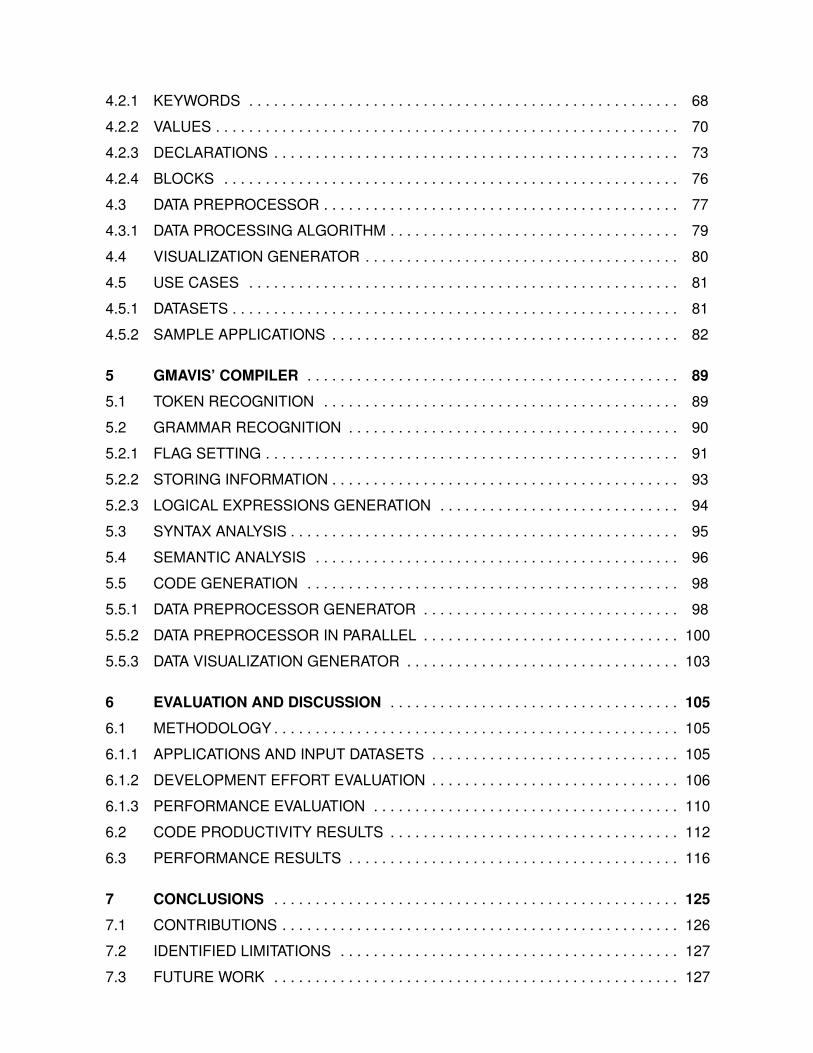
4.2.1 KEYWORDS . . . . . . . . . . . . . . . . . . . . . . . . . . . . . . . . . . . . . . . . . . . . . . . . . . . . 68

4.2.2 VALUES . . . . . . . . . . . . . . . . . . . . . . . . . . . . . . . . . . . . . . . . . . . . . . . . . . . . . . . . 70

4.2.3 DECLARATIONS . . . . . . . . . . . . . . . . . . . . . . . . . . . . . . . . . . . . . . . . . . . . . . . . . 73

4.2.4 BLOCKS . . . . . . . . . . . . . . . . . . . . . . . . . . . . . . . . . . . . . . . . . . . . . . . . . . . . . . . 76

4.3 DATA PREPROCESSOR . . . . . . . . . . . . . . . . . . . . . . . . . . . . . . . . . . . . . . . . . . . 77

4.3.1 DATA PROCESSING ALGORITHM . . . . . . . . . . . . . . . . . . . . . . . . . . . . . . . . . . . 79

4.4 VISUALIZATION GENERATOR . . . . . . . . . . . . . . . . . . . . . . . . . . . . . . . . . . . . . . 80

4.5 USE CASES . . . . . . . . . . . . . . . . . . . . . . . . . . . . . . . . . . . . . . . . . . . . . . . . . . . . 81

4.5.1 DATASETS . . . . . . . . . . . . . . . . . . . . . . . . . . . . . . . . . . . . . . . . . . . . . . . . . . . . . . 81

4.5.2 SAMPLE APPLICATIONS . . . . . . . . . . . . . . . . . . . . . . . . . . . . . . . . . . . . . . . . . . 82

5 GMAVIS’ COMPILER . . . . . . . . . . . . . . . . . . . . . . . . . . . . . . . . . . . . . . . . . . . . . 89

5.1 TOKEN RECOGNITION . . . . . . . . . . . . . . . . . . . . . . . . . . . . . . . . . . . . . . . . . . . 89

5.2 GRAMMAR RECOGNITION . . . . . . . . . . . . . . . . . . . . . . . . . . . . . . . . . . . . . . . . 90

5.2.1 FLAG SETTING . . . . . . . . . . . . . . . . . . . . . . . . . . . . . . . . . . . . . . . . . . . . . . . . . . 91

5.2.2 STORING INFORMATION . . . . . . . . . . . . . . . . . . . . . . . . . . . . . . . . . . . . . . . . . . 93

5.2.3 LOGICAL EXPRESSIONS GENERATION . . . . . . . . . . . . . . . . . . . . . . . . . . . . . 94

5.3 SYNTAX ANALYSIS . . . . . . . . . . . . . . . . . . . . . . . . . . . . . . . . . . . . . . . . . . . . . . . 95

5.4 SEMANTIC ANALYSIS . . . . . . . . . . . . . . . . . . . . . . . . . . . . . . . . . . . . . . . . . . . . 96

5.5 CODE GENERATION . . . . . . . . . . . . . . . . . . . . . . . . . . . . . . . . . . . . . . . . . . . . . 98

5.5.1 DATA PREPROCESSOR GENERATOR . . . . . . . . . . . . . . . . . . . . . . . . . . . . . . . 98

5.5.2 DATA PREPROCESSOR IN PARALLEL . . . . . . . . . . . . . . . . . . . . . . . . . . . . . . . 100

5.5.3 DATA VISUALIZATION GENERATOR . . . . . . . . . . . . . . . . . . . . . . . . . . . . . . . . . 103

6 EVALUATION AND DISCUSSION . . . . . . . . . . . . . . . . . . . . . . . . . . . . . . . . . . . 105

6.1 METHODOLOGY . . . . . . . . . . . . . . . . . . . . . . . . . . . . . . . . . . . . . . . . . . . . . . . . . 105

6.1.1 APPLICATIONS AND INPUT DATASETS . . . . . . . . . . . . . . . . . . . . . . . . . . . . . . 105

6.1.2 DEVELOPMENT EFFORT EVALUATION . . . . . . . . . . . . . . . . . . . . . . . . . . . . . . 106

6.1.3 PERFORMANCE EVALUATION . . . . . . . . . . . . . . . . . . . . . . . . . . . . . . . . . . . . . 110

6.2 CODE PRODUCTIVITY RESULTS . . . . . . . . . . . . . . . . . . . . . . . . . . . . . . . . . . . 112

6.3 PERFORMANCE RESULTS . . . . . . . . . . . . . . . . . . . . . . . . . . . . . . . . . . . . . . . . 116

7 CONCLUSIONS . . . . . . . . . . . . . . . . . . . . . . . . . . . . . . . . . . . . . . . . . . . . . . . . . 125

7.1 CONTRIBUTIONS . . . . . . . . . . . . . . . . . . . . . . . . . . . . . . . . . . . . . . . . . . . . . . . . 126

7.2 IDENTIFIED LIMITATIONS . . . . . . . . . . . . . . . . . . . . . . . . . . . . . . . . . . . . . . . . . 127

7.3 FUTURE WORK . . . . . . . . . . . . . . . . . . . . . . . . . . . . . . . . . . . . . . . . . . . . . . . . . 127

REFERENCES . . . . . . . . . . . . . . . . . . . . . . . . . . . . . . . . . . . . . . . . . . . . . . . . . . 129

APPENDIX A – Performance Results (Raw) . . . . . . . . . . . . . . . . . . . . . . . . . . . . 135

APPENDIX B – GMaVis EBNF Grammar . . . . . . . . . . . . . . . . . . . . . . . . . . . . . . 141

27

1. INTRODUCTION

Data generation has increased exponentially in recent years. In 2002, about fiveexabytes were electronically transferred [LV15]. In 2007, the amount of digital data pro-duced in a year surpassed the world’s data storage capacity for the first time. Then in 2009,800 exabytes of data were generated [MCB+11]. The International Data Corporation (IDC)1

estimates that this volume may grow about 44 times by 2020, which implies a 40 percentrate of annual growing. Many fields such as social networks, government data, health care,and stock market keep producing this data and increase its production every year world-wide [ZH13].

Big data analysis provide interesting information that can help in decision-making.Currently, there are many techniques to perform big data analysis and help users to gainquicker insights. Among these techniques, it is possible to highlight: artificial and biologicalneural networks; models based on the principle of the organization; methods of predictiveanalysis; statistics; natural language processing; data mining; optimization and data visu-alization [ZH13]. All of these techniques can extract information/knowledge and producepredictions to help people in decision making. Furthermore, big data analysis can empowerthe scientific and general community to solve problems, create new products, identify poten-tial innovation, and improve people’s lives. Moreover, it is currently used in many areas likebiology, health, finance, social networking and other fields that require its advantages.

Data visualization is an efficient and powerful technique used in big data anal-ysis. It has an advantage over other techniques because the human brain can processvisual elements faster than texts/values. The human perception system processes an im-age in parallel while texts and values are limited to a sequential reading process [WGK10].Consequently, data visualization is very useful for big data analysis, since it facilitates andaccelerates the human understanding of data/information. Information representation usinggraphical elements has evolved, and it has been used in several areas to increase humanperception [Gha07].

1.1 Motivation

In a simplified way, the visualization pipeline, explained in Chapter 2, has three mainstages. The first one is the data pre-processing phase that includes data modeling and se-lection. The second one is data to visual mappings, which covers the mapping of the data tovisual structures. The last stage is the view transformation, which refers to the users interac-tions on the visualization [WGK10]. Current tools that enable the creation of geospatial data

1http://www.idc.com/

28

visualization do not provide abstraction of complexities for the first phase. Thus, althoughbig data visualization offers many benefits, its production is still a challenge [ZCL13]. Userswith a low-level knowledge of software development may have a hard time for creating aninformation visualization for a large amount of data, because it requires high cost and effortin programming to process and manipulate large volumes of data. Most current tools requireat least some computer programming knowledge, even when using high-level interface li-braries/tools (e.g., Google Charts, Leaflet, OpenLayers, Processing, etc.). Therefore, whendomain users are dealing with big datasets or huge files, they need to implement or use athird software or tool to preprocess data before the visualization creation. These tasks takeconsiderable time that users could use to focus on domain problems.

Since a visualization creation for a vast amount of data requires a high compu-tational cost in processing, parallel programming can be explored to achieve better perfor-mance. Parallel programming enables applications to take advantage of parallel architec-tures by dividing the data or the processing to perform in several processor unities [RR13].Thus, the main advantages of parallel programming are reducing execution time and improv-ing performance by performing more tasks or processing more data in less time. Currently,there are many parallel computer architectures such as multi-core/GPU workstations, clus-ters, and grids. Today, even simple workstations have multiple processing units and this typeof architecture is extremely accessible for any domain user. Hence, exploring these com-puter architectures through parallel programming is essential to reach better performance incomputing.

Nevertheless, taking advantage of parallelism is a difficult task because it requiresanalysis of some factors. These factors may influence the process of software paralleliza-tion. For example, it is essential to choose a computer system architecture, analyze thesoftware problem, select the parallel programming model that best fit the problem, learnabout a parallel programming interface, and other tasks. Decisions must also be madeduring development that may change the final product, sometimes achieving unexpectedresults such as unsatisfactory performance. Parallel programming also requires another setof considerations, such as how the software will handle memory, data dependency, commu-nication, input/output of data, synchronization, interface that better solve the problem, andhow data/tasks will be split. Thus, parallel programming is also a hard task for domain users,since they have to deal with low-level programming and understand many questions in thisarea to extract the maximum performance of parallel computers.

29

1.2 Research Scenario

GMaVis and this work contributes to a framework built at GMAP2 research group.It is the result of a set of researches and works developed in the research group that has asmain objective to facilitate the creation and implementation of parallel applications. GMaViswas built on top of this framework, at the application level, generating SPar [Gri16] annota-tions and using its compiler to generate a parallel data preprocessor. Figure 1.1 illustratesthis framework.

Figure 1.1 – Research scenario framework (Extracted from [Gri16]).

SPar is a domain-specific language that allows the parallelism of code using anno-tations and the implementation of parallel processing based on stream parallelism. SPar wasproposed to address stream processing applications. It is a C++ embedded domain-specificlanguage (DSL) for expressing stream parallelism by using standard C++11 attribute anno-tations. It introduces high-level parallel abstractions for developing stream based parallelprograms as well as reducing sequential source code rewriting. Spar allows C++ developersto express stream parallelism by using the standard syntax grammar of the host language. Italso enables minimal sequential code rewriting thus reducing the effort needed to programthe parallel application. Additionally, SPar provides flexibility for annotating the C++ sequen-tial code in different ways. In the DSL Generation Engine, Cincle, a compiler infrastructure fornew C/C++ language extensions enables SPar compiler to generate code to FastFlow andMPI (Message Passing Interface) that takes advantage of different architecture systems.

Therefore, SPar simplified the parallelization of the data preprocessor module byenabling GMaVis to compile the same code for both parallel or sequential execution by justmodifying a compiler argument. GMaVis used the same code as the sequential version

2www.inf.pucrs.br/gmap

30

annotated in order to generate parallel version with SPar compiler. Also, it enabled GMaVisto easily abstract the parallel programming completely from users. Thus, domain users willnot have to worry about creating parallel programming code to speed up data processingduring visualization creation.

1.3 Objectives and Contributions

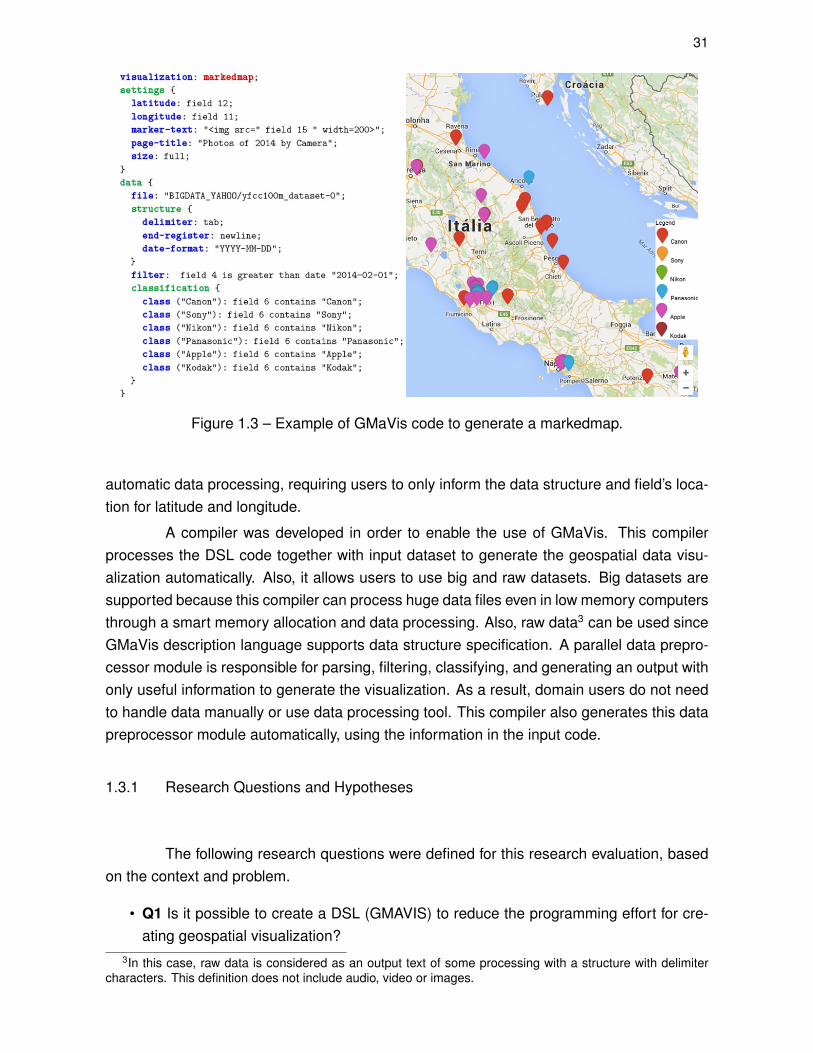
Considering this context, the main goal of this work is to present and describeGMaVis [LGMF15], an external domain-specific language (DSL) that facilitates the creationof visualization of geospatial information by using multi-core architectures to process datain parallel. Its compiler abstracts complexities from the whole visualization creation pro-cess, even in the data pre-processing phase. Also, it allows domain users with low-levelknowledge in computer programming to create these visualizations through a high-level de-scription language. These users can easily do it with a few lines of code, using simpledeclarations and blocks to express visualization details. Currently, GMaVis supports thecreation of three types of geospatial visualization: markedmap, clusteredmap and heatmap.Figures 1.2 and 1.3 illustrate the GMaVis source code required to create a heatmap anda markedmap, respectively. These examples show that GMaVis has a short and simplegrammar, enabling users to create a visualization with a few lines of code.

Figure 1.2 – Example of GMaVis code to generate a heatmap.

Furthermore, GMaVis provides declarations to create filters and classes. Thesedeclarations can be used to select data, remove registers, apply data classification, high-light specific values, and create legends with symbols and classification description. Also, itincludes delimiter specification that enables the use of raw datasets as input. In this case,GMaVis parses the input data using the specified delimiters. Moreover, this DSL provides

31

Figure 1.3 – Example of GMaVis code to generate a markedmap.

automatic data processing, requiring users to only inform the data structure and field’s loca-tion for latitude and longitude.

A compiler was developed in order to enable the use of GMaVis. This compilerprocesses the DSL code together with input dataset to generate the geospatial data visu-alization automatically. Also, it allows users to use big and raw datasets. Big datasets aresupported because this compiler can process huge data files even in low memory computersthrough a smart memory allocation and data processing. Also, raw data3 can be used sinceGMaVis description language supports data structure specification. A parallel data prepro-cessor module is responsible for parsing, filtering, classifying, and generating an output withonly useful information to generate the visualization. As a result, domain users do not needto handle data manually or use data processing tool. This compiler also generates this datapreprocessor module automatically, using the information in the input code.

1.3.1 Research Questions and Hypotheses

The following research questions were defined for this research evaluation, basedon the context and problem.

• Q1 Is it possible to create a DSL (GMAVIS) to reduce the programming effort for cre-ating geospatial visualization?

3In this case, raw data is considered as an output text of some processing with a structure with delimitercharacters. This definition does not include audio, video or images.

32

• Q2 Can the parallel code generated by this DSL speed up the data processing of rawgeospatial data?

With these two research questions, some hypotheses were considered. H1 and H2are related to Q1, and H3 and H4 were defined in respect to Q2.

• H1 GMaVis requires less programming effort than visualization libraries (Google MapsAPI, Leaflet and OpenLayers).

• H2 The inclusion of automatic data pre-processing in GMaVis reduces programmingeffort.

• H3 GMaVis can generate parallel code annotations using SPar for speeding up perfor-mance.

• H4 Code generation for SPar is simpler than using TBB (Thread Building Blocks) forspeeding up performance.

This work has three main contributions described as follows:

• First, it offered a high-level interface that abstracts all raw data pre-processing, pro-gramming elements (i.e., functions, variables, and expressions), visualization genera-tion and parallel programming as a whole.

• Second, it presents an efficient internal data preprocessor module, which has enabledthe processing of huge data files on computers with low memory specifications.

• Third, it presents a method for generating visualizations automatically through a simpledescription language, with total abstraction of parallel programming and low level pro-gramming. Also, this work includes the implementation of a compiler to receive bothsource code and data to generate the visualization automatically.

We evaluated the DSL using programming effort and performance approaches.First we wanted to know if GMaVis could increase code productivity and reduce the ef-fort required to implement a geospatial data visualization from scratch. Also, we verified ifit would be possible to increase performance with a parallel version of data preprocessormodule. Results from programming effort analysis showed that GMaVis can reduce the ef-fort for developing geospatial data visualization since it requires less lines of code than otherlibraries. Moreover, it does not need an extra effort to preprocess data before the visual map-ping and display phases of visualization creation, abstracting complexities from the wholevisualization creation process. Performance results exposes that GMaVis achieved less exe-cution time and higher throughput rates to preprocess data using parallel processing. Also, acomparison of data preprocessors parallelized using SPar and TBB [Rei07] presented highthroughput and less execution time when using SPar working with big datasets. In someapplications, TBB performed in less time with small datasets.

33

1.4 Thesis Organization

The remainder of this work is organized in the following way. Chapter 2 presentssome background concepts related with this research. Chapter 3 introduces and comparesthe most important related works. Chapter 4 details the proposed domain-specific languageand Chapter 5 explains its implemented compiler. Chapter 6 presents the methodology andevaluation results. Finally, Chapter 7 presents the final considerations and future works.

34

35

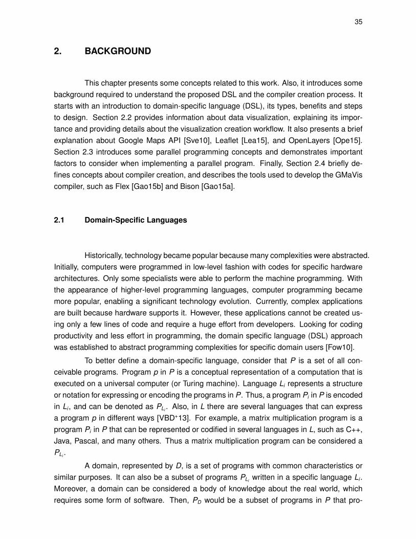
2. BACKGROUND

This chapter presents some concepts related to this work. Also, it introduces somebackground required to understand the proposed DSL and the compiler creation process. Itstarts with an introduction to domain-specific language (DSL), its types, benefits and stepsto design. Section 2.2 provides information about data visualization, explaining its impor-tance and providing details about the visualization creation workflow. It also presents a briefexplanation about Google Maps API [Sve10], Leaflet [Lea15], and OpenLayers [Ope15].Section 2.3 introduces some parallel programming concepts and demonstrates importantfactors to consider when implementing a parallel program. Finally, Section 2.4 briefly de-fines concepts about compiler creation, and describes the tools used to develop the GMaViscompiler, such as Flex [Gao15b] and Bison [Gao15a].

2.1 Domain-Specific Languages

Historically, technology became popular because many complexities were abstracted.Initially, computers were programmed in low-level fashion with codes for specific hardwarearchitectures. Only some specialists were able to perform the machine programming. Withthe appearance of higher-level programming languages, computer programming becamemore popular, enabling a significant technology evolution. Currently, complex applicationsare built because hardware supports it. However, these applications cannot be created us-ing only a few lines of code and require a huge effort from developers. Looking for codingproductivity and less effort in programming, the domain specific language (DSL) approachwas established to abstract programming complexities for specific domain users [Fow10].

To better define a domain-specific language, consider that P is a set of all con-ceivable programs. Program p in P is a conceptual representation of a computation that isexecuted on a universal computer (or Turing machine). Language Li represents a structureor notation for expressing or encoding the programs in P. Thus, a program Pi in P is encodedin Li , and can be denoted as PLi . Also, in L there are several languages that can expressa program p in different ways [VBD+13]. For example, a matrix multiplication program is aprogram Pi in P that can be represented or codified in several languages in L, such as C++,Java, Pascal, and many others. Thus a matrix multiplication program can be considered aPLi .

A domain, represented by D, is a set of programs with common characteristics orsimilar purposes. It can also be a subset of programs PLi written in a specific language Li .Moreover, a domain can be considered a body of knowledge about the real world, whichrequires some form of software. Then, PD would be a subset of programs in P that pro-

36

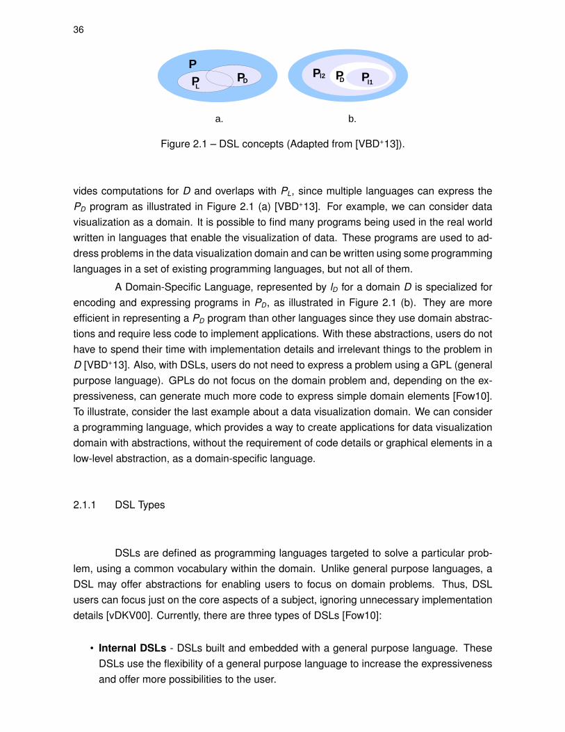
Figure 2.1 – DSL concepts (Adapted from [VBD+13]).

vides computations for D and overlaps with PL, since multiple languages can express thePD program as illustrated in Figure 2.1 (a) [VBD+13]. For example, we can consider datavisualization as a domain. It is possible to find many programs being used in the real worldwritten in languages that enable the visualization of data. These programs are used to ad-dress problems in the data visualization domain and can be written using some programminglanguages in a set of existing programming languages, but not all of them.

A Domain-Specific Language, represented by lD for a domain D is specialized forencoding and expressing programs in PD, as illustrated in Figure 2.1 (b). They are moreefficient in representing a PD program than other languages since they use domain abstrac-tions and require less code to implement applications. With these abstractions, users do nothave to spend their time with implementation details and irrelevant things to the problem inD [VBD+13]. Also, with DSLs, users do not need to express a problem using a GPL (generalpurpose language). GPLs do not focus on the domain problem and, depending on the ex-pressiveness, can generate much more code to express simple domain elements [Fow10].To illustrate, consider the last example about a data visualization domain. We can considera programming language, which provides a way to create applications for data visualizationdomain with abstractions, without the requirement of code details or graphical elements in alow-level abstraction, as a domain-specific language.

2.1.1 DSL Types

DSLs are defined as programming languages targeted to solve a particular prob-lem, using a common vocabulary within the domain. Unlike general purpose languages, aDSL may offer abstractions for enabling users to focus on domain problems. Thus, DSLusers can focus just on the core aspects of a subject, ignoring unnecessary implementationdetails [vDKV00]. Currently, there are three types of DSLs [Fow10]:

• Internal DSLs - DSLs built and embedded with a general purpose language. TheseDSLs use the flexibility of a general purpose language to increase the expressivenessand offer more possibilities to the user.

37

• External DSLs - Address DSLs that have their own grammar, without any generalpurpose language as host. These DSLs usually have simple grammar and focus onoffering high-level programming language interfaces for the user. On the other hand,users will need to learn a new language and may have limited expressiveness.

• Workbench DSLs - These are non-textual DSLs that use graphic representations fordevelopment through an interface development environment (IDE). With a workbenchDSL, users can easily visualize the domain problems with visual elements such asspreadsheets, graphical models, and shapes. Also, some domain experts may feelmore comfortable manipulating visual elements than source code [Gho10].

2.1.2 Advantages in Using DSLs

The use of DSLs to address domain problems provides some benefits [MHS05].First, it allows better software specification, development and maintenance. Usually, thelanguage interface is created based on the domain problem and has a grammar with avocabulary closer to the domain, with terms and commonly used words. It facilitates theunderstanding of code even for non-developers. Also, DSL packaging abstract implementa-tion details allow users to focus on important questions to solve their problems. Moreover, itenables efficiency, since a DSL reduces the required effort to write or modify a code, and thecommunication between developers and domain users is improved. Thus, it provides highconsistency of applications with software specifications.

DSLs allow software to be expressed using a friendly language, at the same ab-straction level of the domain problem. This enables domain experts to understand, verify,change and develop their software by themselves, without requiring experienced develop-ers with specific knowledge in computer programming. Furthermore, this empower domainusers and enables the creation of high quality applications because domain experts, whohave a deeper knowledge about domain problems, can make improvements.

2.1.3 DSL’s Design and Implementation

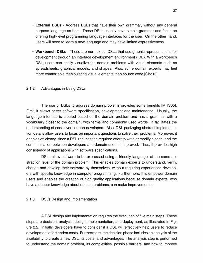
A DSL design and implementation requires the execution of five main steps. Thesesteps are decision, analysis, design, implementation, and deployment, as illustrated in Fig-ure 2.2. Initially, developers have to consider if a DSL will effectively help users to reducedevelopment effort and/or costs. Furthermore, the decision phase includes an analysis of theavailability to create a new DSL, its costs, and advantages. The analysis step is performedto understand the domain problem, its complexities, possible barriers, and how to improve

38

and facilitate domain users to solve their problems through a DSL. Also, it determines whichtype of DSL the domain users expect. Moreover, to avoid costs and time-consumption, thisstep includes a study concerning existing DSLs, to see if it is possible to use an existing DSLinstead of creating a new from scratch [MHS05].

Figure 2.2 – DSL design steps (Adapted from [MHS05]).

The third step is the design, where the DSL creator will make decisions aboutimplementation aspects that will influence the whole DSL cycle life. For example, it canstart with the decision about creating an external or internal DSL. Creating an internal DSLenables the use of an existing familiar programming language for domain users, requiringless effort from users in the learning process. However, when users do not know abouta GPL, implementing an internal DSL will require more time for users because they willhave to learn both the GPL and the DSL. Also, in this step, the DSL developer will specifythe vocabulary, grammar, transformation rules, DSL architecture, and additional libraries ortools. The next step is the implementation, which includes the creation of the DSL softwarethat will enable users to generate applications. In this phase, the compiler or interpreter, andthe whole DSL architecture will be implemented. Finally, the deployment phase includes theDSL implementation for users [MHS05].

2.2 Data Visualization and Geospatial Data

Data visualization is defined as "the communication of information using graphicalrepresentations" [WGK10]. People use images to express information since before any for-malization in written language. Because the human perception system processes images inparallel, this achieves faster results in finding and extracting information. Sequential read-ing limits learning and information collecting from text or values to a slower process. Thus,visualization techniques are used in daily activities, such as the utilization of a map in anunknown region, a chart of the stock market, an analysis of the human population and inadvertising. In all of these activities, visualizations can provide a representation of textual orverbal information. It can also be used as a complementary alternative to provide a quickand adequate understanding of information [WGK10].

39

Currently, many data visualization tools offer different possibilities to represent data.Usually, these visualization tools are classified by the supported amount or type of data, datarepresentation and its techniques to generate and display. Visualization techniques used inthe creation process depend on the kind of input data [Gha07]. Therefore, there are differentdata visualization techniques that are more appropriate for each data type. It is up to thevisualization creator to choose the best visualization technique for the input data.

Often, the process of creating a data visualization follows a workflow, which, in asimplified way, has three main phases. Figure 2.3 demonstrates this workflow. The firstphase is data pre-processing. It includes an analysis of the input, structure and the kindof data that is being handled. When this data comes from a raw dataset without previousprocessing, data preparation is required to select, filter, classify and remove undesired reg-isters. The second phase is data to visual mappings, where the data elements is mappedinto visual representations, according to the attributes previously selected. Finally, the visu-alization is generated in view transformations. It also includes setting the scene parametersand interactions between the user and the visualization, which allows them to modify detailsand use mechanisms to have a richer experience in data exploration [WGK10]. Users canchange the final visualization by changing information in the three phases according to theirprogramming and data manipulation knowledge.

Figure 2.3 – Data visualization pipeline (Adapted from [CMS99]).

The process of visualization creation using a large dataset, however, is a hard taskfor users with a low-level of knowledge in computer programming. For example, to createa big data visualization, domain users have to deal with big data processing, analysis, andvisualization algorithms/technologies. Also, depending on the visualization type, data miningalgorithms are fundamental to select, classify, reduce or optimize data. If the visualizationhas some interactivity with users, it will need a parallel interface to process the graphicelements. For all these requirements, users need to look for algorithms, tools, and platformsand learn about them before implementation. Since these users are from science/industryand have limited knowledge of programming languages, this implies a great deal of effort

40

and time to visualize an information from the datasets. This effort is even significant if rawdata is input, which requires pre-processing.

This work focuses on geospatial data visualizations that use a special type of datawhich specifies the location of an object or phenomena in each register, usually throughits Latitude and Longitude. Examples of geospatial data are global climate modeling, envi-ronmental records, economic and social measures and indicators, customer analysis, andcrime data. The strategy used to represent this kind of data is to map the spatial attributesdirectly to a 2D map visualization [WGK10].

Some libraries allow users to create geospatial data visualizations, such as GoogleMaps API, OpenLayers, and Leaflet. When using these libraries, it is up to the user to pre-process the data in the correct format. Furthermore, for massive data, it is often requiredto create a software to process it automatically and provide an output file with the formatused in the library. Figure 4.1(a) shows the workflow of traditional libraries to generate a vi-sualization. The dotted line around Generation of the Visualization and Library Format Datademonstrate the supporting scope of these libraries without needing extra programming bythe user. Because we used these libraries in this work, each one will be briefly explainedbellow.

2.2.1 Google Maps API

Introduced by Google in 2005, this API improved the use of maps on the web,allowing users to drag and interact to find information. Basically, Google Maps API usesHTML, CSS, and JavaScript to display the map and its elements. This API use tiles, whichare small pieces of images, to create a full map. Initially, tiles are loaded in the backgroundwith Ajax calls. Then these are inserted into <div>tags in an HTML page. When the userinteracts with a created map with the Google Maps API, it sends coordinates and detailedinformation to a server, and this provides with new tiles that load on the map [Sve10].

To create a data visualization maps using the Google MAPs API, users must havesome knowledge of JavaScript to create variables, objects and functions. For example, thesteps to generate a simple map are the following. Initially, it requires the inclusion of thelibrary in the HTML file through a URL. Also, a map object may be declared and associatedwith a previously created variable. This object receives some information, as initial position,zoom, layers and the div element which will receive the map in HTML code. Finally, usersneed to have data to insert in this visualization. For a marked map, each marker requires,at least, three lines of code to generate an object with latitude and longitude information.If a classification is desired, such as to change marker colors or sizes, users may insert avariable receiving another object with an icon declaration.

41

For a better understanding of data visualization creation using this library, somepieces of code are presented as examples. Because of the number of lines occupied, we donot show the additional HTML and JavaScript code, focusing just on the Google Maps APIcode required to create the data visualization. The Listing 2.1 presents how to build a mapwith markers using Google Maps API.

1 / / HTML CODE ( wi th API d e c l a r a t i o n and requ i red elements )2

3 var map = new google . maps .Map( document . getElementById ( ’map ’ ) , {4 zoom : 6 ,5 center : new google . maps . LatLng (54 , 12) ;6 mapTypeId : google . maps . MapTypeId .ROADMAP,7 } ) ;8

9 / / . . . Data . . .10 var marker = new google . maps . Marker ( { / / This piece of code i s r e p l i c a t e d11 p o s i t i o n : new google . maps . LatLng (54 , 12) , / / f o r each a d d i t i o n a l marker i nse r t ed .12 map: map13 } ) ;14 / / . . . Data . . .15

16

17 / / HTML CODE ( Body )

Listing 2.1 – Map creation with Google Maps API [Sve10].

When a developer wants to insert a new marker on the map, he must add the dataand its code in lines 10 and 13 of the Listing 2.1. Note that, for each marker inserted in themap, the developer needs to replicate this piece of code, modifying the information aboutlatitude and longitude. If this data visualization handles a large volume of data, then the finalcode will be large, considering the numbers of lines. Also, the Google Maps API does notprovide a feature to process data automatically. It requires users to handle data manuallyor use an external tool to process data before it is inserted into JavaScript declarations andput in the HTML code. The previous example showed a code to create a simple map withone marker. However, if a user needs to create one with one hundred markers, each dataelement would have to be determined and inserted into the JavaScript code, replicating themarker variable. This task may increase the effort to create the map and, depending onthe quantity of data, it would require the use of external tools or software development toperform this activity.

2.2.2 OpenLayers

OpenLayers is an open source JavaScript library that provides features for display-ing map data in web browsers. It also provides an API for building web-based geographicapplications. Furthermore, it offers a set of components, such as maps, layers, or controls.

42

OpenLayers offers access to a great number of data sources using many different data for-mats. Moreover, it implements many standards from Open Geospatial Consortium1 [Ope15].

Similar to the Google Maps API, OpenLayers also requires the library declarationin the HTML file. The process for creating a simple map with OpenLayers is similar to thatpresented in the Google Maps API. First a declaration of an object to a map with details andinformation must be given to create the visualization. In OpenLayers, the creation of at leastone layer is required. A layer is a feature in OpenLayers that allows for the implementationof different types of data visualization in a single file. For example, it enables the creationof a heatmap with markers using two layers. However, when creating a simple map withmarkers, it modifies the insertion of markers on the map. Here, each marker will not only becreated but also associated with a layer.

1 / / HTML CODE ( wi th API d e c l a r a t i o n and requ i red elements )2 var map = new o l .Map ( {3 t a r g e t : ’map ’ ,4 l aye rs : [ new o l . l a ye r . T i l e ( { source : new o l . source . MapQuest ( { l a ye r : ’ sa t ’ } ) } ) ] ,5 view : new o l . View ( {6 center : o l . p r o j . t rans form ( [ 5 4 . 4 1 , 12 .82 ] , ’EPSG:4326 ’ , ’EPSG:3857 ’ ) ,7 zoom : 48 } )9 } ) ;

10 var markers = new OpenLayers . Layer . Markers ( " Markers " ) ;11 map. addLayer ( markers ) ;12

13 / / Data . . .14 var lonLa t = new OpenLayers . LonLat ( −89.461412 , 30.912627) / / This piece of code i s r e p l i c a t e d15 . t rans form ( / / f o r each a d d i t i o n a l marker i nse r t ed .16 new OpenLayers . P r o j e c t i o n ( "EPSG:4326 " ) ,17 map. ge tP ro jec t i onOb jec t ( )18 ) ;19 / / Data . . .20

21 markers . addMarker (new OpenLayers . Marker ( lonLa t ) ) ;22 / / HTML CODE ( Body )

Listing 2.2 – Layer creation with OpenLayers library [Ope15].

Listing 2.2 presents an example code for creating a simple map with one marker.In the first lines, it has the map specification with details about centering, position, tiles andzoom. Then, a layer called markers is declared in line 10. This layer receives the markers inthe following lines of code. As in the first example with the Google Maps API, here the codeto insert a marker is also replicated. Thus, users will need to handle their data manually oruse an external tool to process data before creating the visualization.

2.2.3 Leaflet

Leaflet is an open-source JavaScript library used to create interactive maps. Leafletworks by taking advantage of HTML5 and CSS3 [Lea15] to implement maps and display vi-

1http://www.opengeospatial.org

43

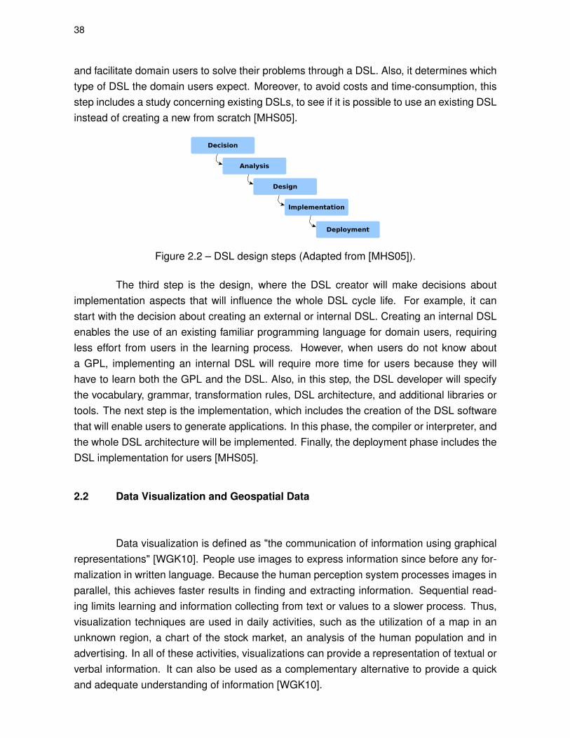
sual elements. Similar to the previous libraries, it allows for the creation of maps usinggeospatial data. Moreover, it provides and supports many features that enable implementa-tion of maps with detailed specifications, since it offers tile layers, markers, popups, vectorlayers, polylines, polygons, circles, rectangles, circle markers, GeoJSON layers, image over-lays, WMS layers and layer groups. Listing 2.3 demonstrates how a simple map with onemarker is created using Leaflet library.

1 / / HTML CODE ( wi th API d e c l a r a t i o n and requ i red elements )2

3 var map = L .map( ’map ’ ) . setView ( [51 .505 , −0.09] , 13) ;4

5 L . t i l e L a y e r ( ’ h t t p : / / { s } . t i l e . osm . org / { z } / { x } / { y } . png ’ , {6 a t t r i b u t i o n : ’&copy ; <a h re f =" h t t p : / / osm . org / copy r i gh t ">OpenStreetMap </a> c o n t r i b u t o r s ’7 } ) . addTo (map) ;8

9 / / Data . . .10 L . marker ( [ 5 1 . 5 , −0.09]) . addTo (map) / / This piece of code i s r e p l i c a t e d11 . bindPopup ( ’A p r e t t y CSS3 popup . <br > Eas i l y customizable . ’ ) / / f o r each a d d i t i o n a l marker

i nse r t ed .12 . openPopup ( ) ;13 / / Data . . .14

15

16 / / HTML CODE ( Body )

Listing 2.3 – Map creation with Leaflet library [Lea15]

The marker and map creation process in Leaflet is similar to other libraries. Initiallythe HTML file is inserted into the library. Next a variable that instantiates a map object iscreated. Another variable then instantiates a marker object given a geographical point andthis marker is added to the map. Finally, an option in this instantiation is declared, whichallows the specification of a text to be shown when a marker is clicked. As in other libraries,the user must have knowledge of JavaScript programming to create a data visualizationmap. Also, the user will need to process and format data before inserting it into the code.

2.3 Parallel Programming

The performance of microprocessor has increased about 50% per year between1986 and 2002 [Pac11]. This increase in performance of single core computers generatedan expectation in users for the next generations of processors. However, the improvementsin performance reduced about 20% after 2002 [Pac11], because single core processors andthe monolithic design could not support higher clock frequencies without a high level of heatand power consumption. Therefore, most manufacturers started producing their processorswith multiple processing units in a single integrated circuit. This enabled manufacturers tokeep increasing the performance and offer fast machines for processing and solving prob-lems with high computational cost, such as climate modeling, protein folding, drug discovery,energy research, and data analysis [Pac11].

44

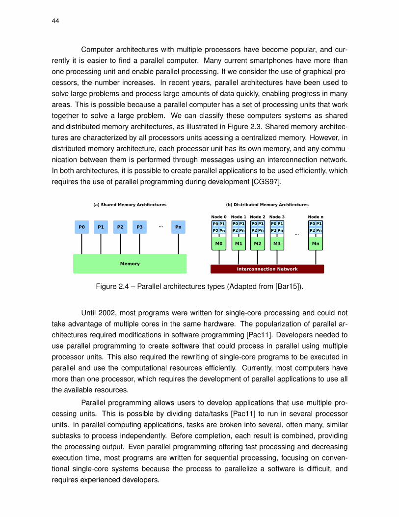
Computer architectures with multiple processors have become popular, and cur-rently it is easier to find a parallel computer. Many current smartphones have more thanone processing unit and enable parallel processing. If we consider the use of graphical pro-cessors, the number increases. In recent years, parallel architectures have been used tosolve large problems and process large amounts of data quickly, enabling progress in manyareas. This is possible because a parallel computer has a set of processing units that worktogether to solve a large problem. We can classify these computers systems as sharedand distributed memory architectures, as illustrated in Figure 2.3. Shared memory architec-tures are characterized by all processors units acessing a centralized memory. However, indistributed memory architecture, each processor unit has its own memory, and any commu-nication between them is performed through messages using an interconnection network.In both architectures, it is possible to create parallel applications to be used efficiently, whichrequires the use of parallel programming during development [CGS97].

Figure 2.4 – Parallel architectures types (Adapted from [Bar15]).

Until 2002, most programs were written for single-core processing and could nottake advantage of multiple cores in the same hardware. The popularization of parallel ar-chitectures required modifications in software programming [Pac11]. Developers needed touse parallel programming to create software that could process in parallel using multipleprocessor units. This also required the rewriting of single-core programs to be executed inparallel and use the computational resources efficiently. Currently, most computers havemore than one processor, which requires the development of parallel applications to use allthe available resources.

Parallel programming allows users to develop applications that use multiple pro-cessing units. This is possible by dividing data/tasks [Pac11] to run in several processorunits. In parallel computing applications, tasks are broken into several, often many, similarsubtasks to process independently. Before completion, each result is combined, providingthe processing output. Even parallel programming offering fast processing and decreasingexecution time, most programs are written for sequential processing, focusing on conven-tional single-core systems because the process to parallelize a software is difficult, andrequires experienced developers.

45

2.3.1 Exploring Parallelism

Exploring parallelism requires changing a sequential code to execute in parallel.There are many ways to parallelize software, and they all depend on the hardware, how theproblem will be solved, available software, interfaces for parallel programming and the strat-egy that will be used. To organize the parallelization process, some models were definedaccording to the parallelization strategy. A parallel programming model is an abstraction ofhow a system works. It specifies the programmer’s view of a parallel application. Somefactors can influence the decision of which model use, such as architectural design, the lan-guage, compiler, or the available libraries. There are different parallel programming modelsfor the same architecture, and the choice of one depends on the application parallelizationstrategy.

We can classify parallel programs by the strategy used. This strategy is related tothe hardware because different computer architectures require different implementations ofparallel programs. For example, a single computer with a multi-core has a different parallelprogram implementation than a cluster of computers. Thus, parallel programming is intrin-sically related to the hardware. Furthermore, developers that create parallel software mustknow the target computer architecture that will run the program. This is required becausethey must decide between the models that can produce better results and optimize the al-gorithm to extract good performance. The three possible classes for this division based oncomputer architecture are parallel programs that use shared memory, message passing orboth, called hybrid programs [MSM04]. These models are presented bellow.

• Shared Memory The shared memory model shares a common address space inmemory among processes. These processes can read and write in this memory asyn-chronously. There are mechanisms like locks or semaphores that resolve contentions,prevent race conditions, deadlocks and control this access to memory to avoid prob-lems [MSM04]. The advantage of using this model is the facility to implement a parallelprogram because the developer does not need to worry about the communication be-tween processes. If we do not consider hardware implementation, in shared memorymodel all the processes have equal access to the memory. Figure 2.3.1 illustratesthis model where multiple processes access the shared memory for both reading andwriting.

• Message Passing In this model, the processes have their own memory to local andprivate access. This model does not have a global memory for universal access. Thus,the multiple tasks can run on a physical machine or multiple machines connected bya network. This model uses messages for processes to communicate and exchangedata through the network connection. Furthermore, it is complex to implement a par-

46

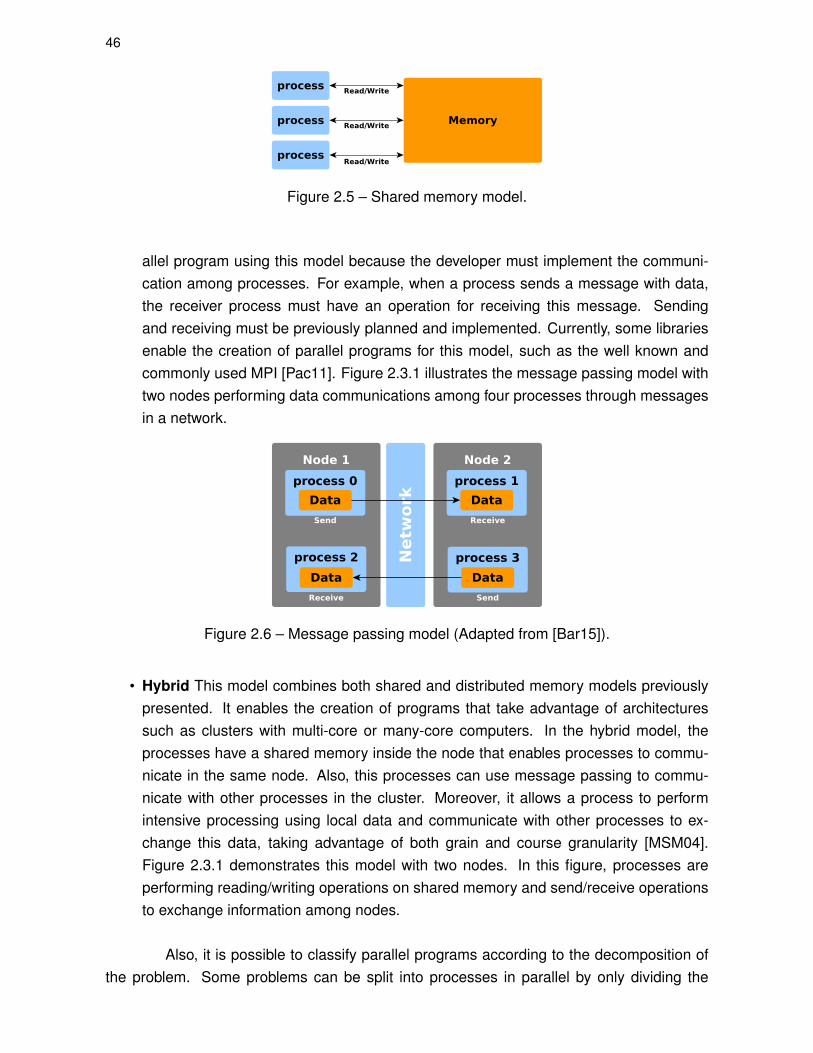
Figure 2.5 – Shared memory model.

allel program using this model because the developer must implement the communi-cation among processes. For example, when a process sends a message with data,the receiver process must have an operation for receiving this message. Sendingand receiving must be previously planned and implemented. Currently, some librariesenable the creation of parallel programs for this model, such as the well known andcommonly used MPI [Pac11]. Figure 2.3.1 illustrates the message passing model withtwo nodes performing data communications among four processes through messagesin a network.

Figure 2.6 – Message passing model (Adapted from [Bar15]).

• Hybrid This model combines both shared and distributed memory models previouslypresented. It enables the creation of programs that take advantage of architecturessuch as clusters with multi-core or many-core computers. In the hybrid model, theprocesses have a shared memory inside the node that enables processes to commu-nicate in the same node. Also, this processes can use message passing to commu-nicate with other processes in the cluster. Moreover, it allows a process to performintensive processing using local data and communicate with other processes to ex-change this data, taking advantage of both grain and course granularity [MSM04].Figure 2.3.1 demonstrates this model with two nodes. In this figure, processes areperforming reading/writing operations on shared memory and send/receive operationsto exchange information among nodes.

Also, it is possible to classify parallel programs according to the decomposition ofthe problem. Some problems can be split into processes in parallel by only dividing the

47

Figure 2.7 – Hybrid model (Adapted from [Bar15]).

data to run on multiple cores. On the other hand, other programs that have multiple taskscan process these in parallel processes. We can divide problem decomposition into dataparallelism and task parallelism. Both models for parallel programming are explained asfollows.

• Data Parallelism: Data parallelism model is characterized by treating the memoryaddress space globally or performing operations on a data set in parallel. This modelorganizes data in a standard structure, for example, an array or cube, and tasks workin parallel on this data structure. During parallel processing, each task works on adifferent part of the same data structure. Usually, tasks perform the same operationon the data, for example, to sum 3 with an array element. However, it can performdifferent operations for each partition of data [Pac11].

• Task Parallelism: This model is most applicable for programs that can break a prob-lem into parallel tasks. This problem can have distinct functions, loops interactionsand costly parts of the code that can be performed in parallel. The objective of thismodel is to divide tasks among cores. If it is applied to programs with few tasks, thedevelopment becomes easier. However, if the problem has many tasks, it can be-come complicated to control the execution of each process, and how it writes or readsmemory without interfering with the result of other tasks [Pac11].

• Stream Parallelism: Stream parallelism is a special kind of task decomposition thathas as characteristic a sequence of tasks. This model can be imagined as an Assemblyline, where data is received as input and a set of operations is performed. However, thisprocessing is organized to receive multiple pieces of data and performs the operationswith a time overlap, resulting in a parallel execution [Bar15].

48

2.3.2 Design of Parallel Programs

Parallelization is used to transform a sequential program into a parallel program tobetter use a parallel system. Parallelism has three main divisions: parallelism at the instruc-tion level, data parallelism, and loop parallelism [RR13]. The systematic way to parallelizecode consists of an initial computation decomposition. In this step, computation dependen-cies are determined in sequential code. Depending on the dependencies in a computation,it can be decomposed into subtasks. Thus, tasks are assigned to processes or threads, andthese are mapped to physical processors or cores [RR13]. However, the problem may bestudied to facilitate the planning and implementation of parallelism. The three typical stepsthat must be performed for software parallelization are:

• Study problem or code: It is important to know how the program works because,when parallelizing software, one must make choices that can change the final result.Moreover, the developer has to guarantee that the parallel program provides the sameresults as the sequential program for the expected input value. Thus, it can be easilyachieved if the developer knows well the problem when developing [Bar15].

• Look for parallelism opportunities: The second step in parallelization is to look forparallelism opportunities. This is easy for experienced developers, but can be hardfor novices. In this step, developers may use a strategy to verify the parts of theprogram that can be decomposed to process in parallel. The developer needs to findconcurrency and decide how to take advantage of it. Also, the developer can breakthe program into tasks, dividing these among processors. Some decisions in this stepcan impact heavily on the development of the parallel version, since sometimes theprogram must be restructured or an entirely new algorithm must be created [Bar15].

• Try to keep all cores busy: When a program is parallelized, the objective is to dividethe processing among the cores/processors to achieve the result in less execution time.If a program is not parallelized correctly, cores can become idle during the processing.A well developed parallelization keeps the cores busy, processing data or tasks toachieve results quickly. It is possible to measure the use of cores through the efficiencycalculus [Bar15].

Synchronization

Determining the sequence processes perform their operations is a critical point toconsider when creating a parallel program. When many processes execute in parallel, andaccess shared spaces in memory, it is important to analyze and examine the sequencesof writing/reading. For example, if two processes read the same value stored in a memory

49

space, and one of the processes changes this value after reading, the final result will beincorrect because the second process will read the modified value. Therefore, in this case,mechanisms must be implemented to control this sequence, making both processes readthe value before the first process modifies it. However, applying this procedure can impactperformance since processes stay idle waiting for a determined process to continue. Also,these mechanisms can serialize some parts of the code. Some procedures to apply controlin synchronization such as lock/semaphore, synchronous communication operations, andbarriers are described below [Pac11].

• Locks/Semaphores: A lock or semaphore is used to serialize and protect the accessto determined global data or a specific piece of code. It works by setting a flag in apiece of data. So, it will be used only by a specific task. Then this unique task cansafely access and modify the protected data. If another task tries to use this dataor code, it will wait until the first task unsets the flag. This operation can affect theperformance, but it is often required when tasks use common data or communicateusing shared memory [Pac11].

• Synchronous through communication: This mechanism is used in parallel pro-grams that communicate between processes. It works by performing blocking commu-nications among processes to coordinate the processing in sequence. For example,a task that may perform an operation will receive a message from another processinforming it that can proceed [Pac11].

• Barriers: This mechanism usually is applied to all the tasks in a parallel program. Itworks by creating a barrier in the code where all the tasks must be achieved to continuethe processing. This enables the synchronization of threads and guarantees that allthe processes execute a procedure at the same time [Pac11].

Data Dependencies

Data dependency is a concept to express when there is a dependence betweenthe order of program operations that affects the results. It is common in shared memorymodels that have multiple processes accessing the same memory location. Usually, a datadependence is an inhibitor of parallelism since one operation needs to be executed afteranother, forcing a sequential execution. An example of data dependency can be seen ina program that needs the result of a previous computation to realize an operation. Andits result will be the input of another operation [Pac11]. In shared memory architectures,data dependency can be handled by the use of synchronization mechanisms. In distributedmemory, it is possible to use communication or barriers for implementing a parallel programwith data dependency [Bar15].

50

Granularity

Granularity is a measure of the ratio of computation versus communication [Bar15].There are two types of granularity: fine-grain parallelism and coarse-grain parallelism. Bothare described bellow.

• Fine-grain Parallelism: This type of granularity has a small number of computationsbetween the communications. This kind of granularity facilitates the implementationof load balancing. However, it is easy to have less performance due to the overheadgenerated by communication. Sometimes, with very fine granularity, it is possible thatcommunication takes more time than processing [Bar15].

• Coarse-grain Parallelism: Represents processing with few communication eventsand a high number of computations. This kind of granularity has more opportunitiesto parallelize and for performance gain. However, it can become hard to handle loadbalancing [Bar15].

I/O

A problem that parallel programmers can face when trying to parallelize code is I/O.Usually, programs that have a lot of I/O operations can be hard to parallelize because loadingor saving data processes can take more time than processing. For example, the reading ofa file from the hard disk can take more time than processing it. Also, saving it can take evenmore time. In this case, the parallelization does not affect performance too much. Currently,some distributed file systems enable parallel I/O operations using distributed computers withreplicated data. In shared memory architectures, it is possible to implement a stream pro-cessing model to process data in small chunks as it is loaded, doing it in a interpolatedtime [Bar15].

2.3.3 Parallel Interfaces

Several parallel programming interfaces allow and facilitate the development of par-allel programs. If we limit this scope for shared-memory architectures, then it is possible tomention: POSIX Threads [NBF96], OpenMP [CJvdP07], FastFlow [ART10], TBB [Rei07],Cilk [Lei09], Intel Parallel Studio [INT15], SPar [Gri16] and many other libraries. These li-braries can be used based on different problems. Table 2.1 describes the target architecturefor each library and the supported parallel programming models. In this analysis, we onlyconsider parallel interfaces that target shared memory, since this is the type of interfaceapplied in this work.

51

Table 2.1 – Comparison of parallel programming interfaces.Interface System

ArchitectureTarget Memory

ArchitectureTask

ParallelismData

ParallelismStream

ParallelismAnnotation

BasedPthreads Multi-core Shared Memory x x xOpenMP Multi-core Shared Memory x x x

Fastflow Multi-core Shared/DistributedMemory x x x

SPar Multi-core /Cluster

Shared/DistributedMemory x x x x

TBB Multi-core Shared Memory x xCilk Multi-core Shared Memory x x xIntel

ParallelStudio

Multi-core Shared Memory x x

2.4 Compilers Creation

A language can be formal or natural. A natural language is a language that hu-man beings use to communicate, which uses a set of symbols and a set of rules that arecombined to communicate information to a group that understands this. On the other hand,a formal language also uses symbols and a set of rules. However, it is designed for ma-chines (programming languages, communication protocols, etc.). Both formal and naturallanguage have a set of rules, called grammar [Kri09], that defines the structure and rules ofthis language.

A compiler is a computer program that reads a language written in a particularprogramming language and translates it into another language. For this operation, a set ofsteps is performed. Initially, a lexical analysis (or linear analysis) is performed to scan theinput code and recognize each language element, creating tokens. After, a syntax analysis(or hierarchical analysis) group the tokens recognized according to a grammar specificationto generate the output during rules matching. The third step in a compilation is the semanticanalysis. It is a verification of the code that tries to find possible semantic errors. Forexample, if a declaration must receive an integer, and the user defines a float number, thisphase will verify and, convert the value to an integer or report a semantic error [ASU06].

Some compilers also have an optimization phase to improve input code after codegeneration. This step usually recognizes possible improvements in the code and changeit to simplify, improve or speed up the compilation product. Finally, the code generation isperformed, which transforms the received code in another language, following transforma-tion rules [ASU06]. This research used Flex and Bison to perform parsing in the GMaViscompiler. Both will be briefly explained next.

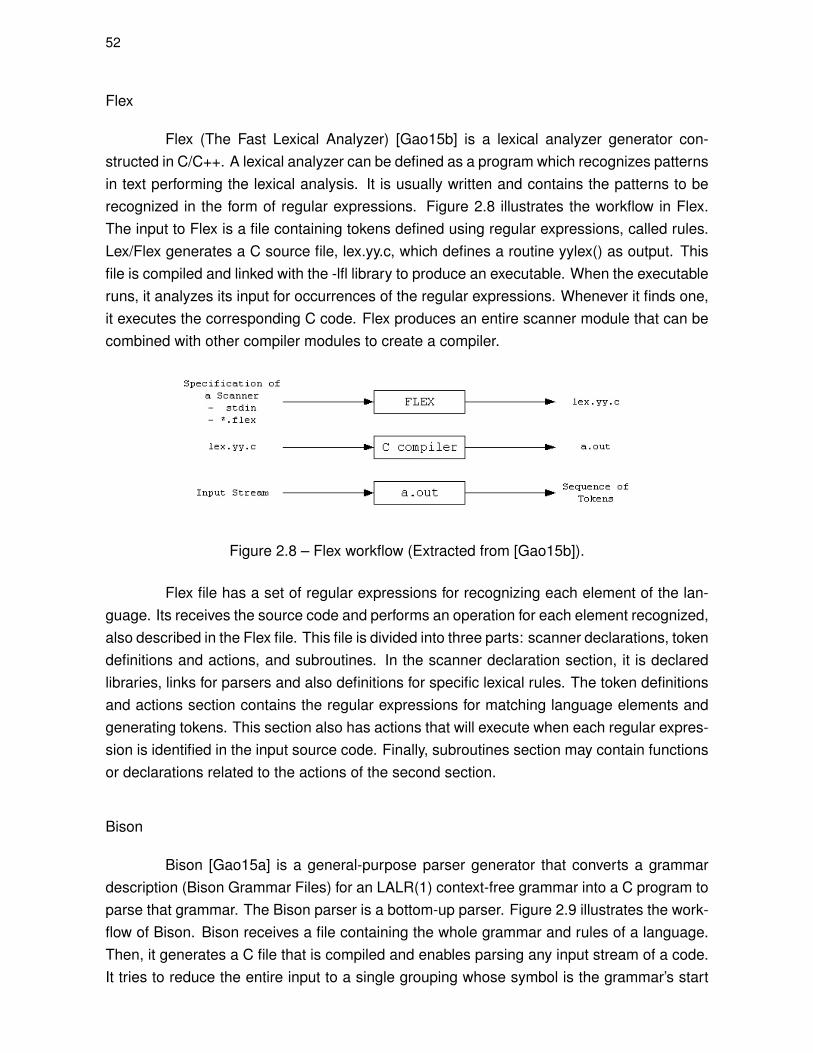
52

Flex

Flex (The Fast Lexical Analyzer) [Gao15b] is a lexical analyzer generator con-structed in C/C++. A lexical analyzer can be defined as a program which recognizes patternsin text performing the lexical analysis. It is usually written and contains the patterns to berecognized in the form of regular expressions. Figure 2.8 illustrates the workflow in Flex.The input to Flex is a file containing tokens defined using regular expressions, called rules.Lex/Flex generates a C source file, lex.yy.c, which defines a routine yylex() as output. Thisfile is compiled and linked with the -lfl library to produce an executable. When the executableruns, it analyzes its input for occurrences of the regular expressions. Whenever it finds one,it executes the corresponding C code. Flex produces an entire scanner module that can becombined with other compiler modules to create a compiler.

Figure 2.8 – Flex workflow (Extracted from [Gao15b]).

Flex file has a set of regular expressions for recognizing each element of the lan-guage. Its receives the source code and performs an operation for each element recognized,also described in the Flex file. This file is divided into three parts: scanner declarations, tokendefinitions and actions, and subroutines. In the scanner declaration section, it is declaredlibraries, links for parsers and also definitions for specific lexical rules. The token definitionsand actions section contains the regular expressions for matching language elements andgenerating tokens. This section also has actions that will execute when each regular expres-sion is identified in the input source code. Finally, subroutines section may contain functionsor declarations related to the actions of the second section.

Bison

Bison [Gao15a] is a general-purpose parser generator that converts a grammardescription (Bison Grammar Files) for an LALR(1) context-free grammar into a C program toparse that grammar. The Bison parser is a bottom-up parser. Figure 2.9 illustrates the work-flow of Bison. Bison receives a file containing the whole grammar and rules of a language.Then, it generates a C file that is compiled and enables parsing any input stream of a code.It tries to reduce the entire input to a single grouping whose symbol is the grammar’s start

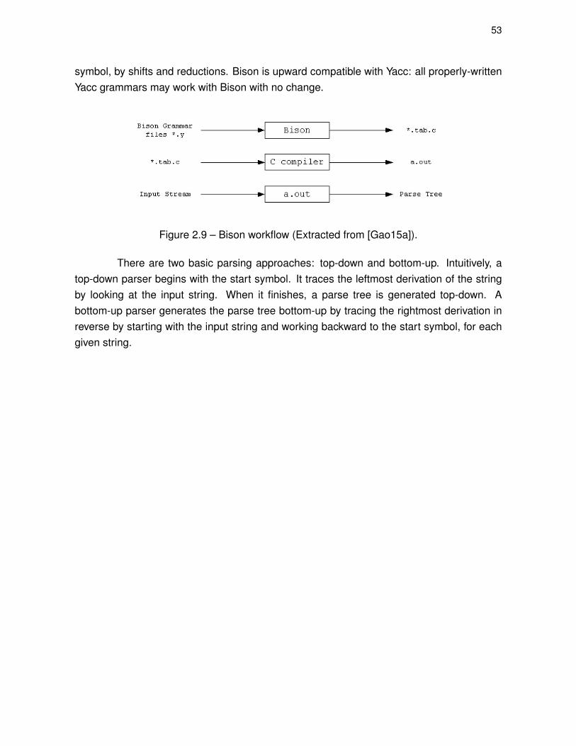
53

symbol, by shifts and reductions. Bison is upward compatible with Yacc: all properly-writtenYacc grammars may work with Bison with no change.

Figure 2.9 – Bison workflow (Extracted from [Gao15a]).

There are two basic parsing approaches: top-down and bottom-up. Intuitively, atop-down parser begins with the start symbol. It traces the leftmost derivation of the stringby looking at the input string. When it finishes, a parse tree is generated top-down. Abottom-up parser generates the parse tree bottom-up by tracing the rightmost derivation inreverse by starting with the input string and working backward to the start symbol, for eachgiven string.

54

55

3. RELATED WORK

This chapter presents some DSLs that were proposed to aid domain users withthe creation of data visualization. Vivaldi [CCQ+er], ViSlang [RBGH14], Diderot [CKR+12],Shadie [HWCP15] and Superconductor [MTAB15] are the DSLs presented in Sections 3.1to 3.5, and the last section contains a comparison between these DSLs and a discussionrelated to this work.

3.1 Vivaldi

In 2013, a domain-specific language called Vivaldi [CCQ+er] was proposed. ThisDSL provides volumetric processing and visualization rendering in parallel using distributedand heterogeneous architectures while providing a high-level language based on Python.With this DSL the user does not need to be concerned with the programming of many-coreprocessors and GPU accelerators. It is because programming software to explore GPUclusters is hard since it requires hardware knowledge and low-level programming. Also,Vivaldi provides standard functions and mathematical operators for customized visualizationand high-throughput image processing applications.

Vivaldi has been designed for ease of use while providing high-throughput perfor-mance supporting distributed heterogeneous architectures. It includes a flexible and high-level programming language, a compiler, and a runtime system. The grammar language issimilar to Python, facilitating its use for domain experts who can focus on application ob-jectives without needing to learn parallel languages such as MPI or CUDA. This DSL alsoabstracts the communication among processes required in parallel programming. A mem-ory model provides a simple and unified view of memory without any data communicationcode required from the users. Data is replicated on different compute nodes while the run-time system performs automatic and transparent synchronization. Also, Vivaldi providesdomain-specific functions and some mathematical operators used in visualization and sci-entific computing to allow users to write customized applications for volume rendering andprocessing.

The target computer architecture that Vivaldi uses is clusters of heterogeneouscomputing nodes (i.e., CPUs and GPUs in each node) on distributed memory system. Vi-valdi abstracts low-level architecture and programming details since it provides abstractionsto manage computing resources and memory using a unified high-level programming en-vironment. Thus, users do not need to have knowledge about CUDA or OpenCL to useGPU because Vivaldi generates parallel GPU code automatically. Also, Vivaldi abstracts

56

MPI communication between nodes and transparently handles memory through a memorymanager in its runtime system. Figure 3.1 illustrates Vivaldi system overview.

Figure 3.1 – Vivaldi system overview (Extracted from [CCQ+er]).

Vivaldi deals with each computing resource (i.e., CPU, GPU) as an independentexecution unit. Each execution unit is assigned an execution ID for processing tasks. Forfunctions, users will define the tasks, input/output data, and task decomposition scheme.The structure of a Vivaldi program is a collection of functions where the main function is thedriver that connects user-defined functions to build a computing pipeline. Therefore, eachfunction call generates a set of tasks that are processed in parallel by available executionunits. As demonstrated in Figure 3.1, the input source code is translated into different typesof native source code. Then, it is saved inside Python main, Python functions, and CUDAfunctions. Tasks are generated based on the main function code. Finally, each task isscheduled to run on one of the execution units depending on the scheduling policy. Low-level data communication and function execution are abstracted and handled by Python,CUDA, and MPI runtime functions.

Figure 3.2 presents a Vivaldi code example and its output. The output visualizationis a volume rendering of a juvenile zebrafish performed on a GPU cluster. It uses an inputtask generation scheme to split and to transfer functions. Brain and nerve systems arerendered in green while other regions are in gray, blue, and red.

57

Figure 3.2 – Vivaldi code and output (Extracted from [CCQ+er]).

3.2 ViSlang

ViSlang [RBGH14] is an interpreted DSL elaborated to offer the possibility of creat-ing scientific visualizations for facilitating its creation by scientists and avoiding the difficultiesof handling a low-level language. A great contribution offered by ViSlang is the possibility ofextending the DSL using slangs. This feature allows the implementation of others DSLs toaddress other issues that are within the domain. Figure 3.3 illustrates the use of slangs.

Figure 3.3 – Slangs in ViSlang (Extracted from [RBGH14]).

ViSlang is a system that decreases the cost of developing new DSLs since it in-tegrates multiple DSLs in one solution to support their flexibility. Figure 3.3 provides anoverview of ViSlang design. ViSlang has a library and an execution environment with sup-port for an extension mechanism. By integrating it into a visualization system, the runtimecan execute commands and change the behavior of the visualization. This runtime performsas a unified programming interface. Internally, DSLs that extend ViSlang are named slangs.It works in the following mode. User input is received and executed by an interpreter. If acommand starts with the keyword using, it will be transmitted to the corresponding slang.Figure 3.3 demonstrates an example code that makes use of the slang renderer. It offers

58

a DSL that allows properties of data mapping to visual elements. This example gives anoverview of the ViSlang runtime system where multiple DSLs are combined using commondata processing and visualization modules. ViSlang currently focuses on processing andvisualization of static volumes. This is not a restriction of the system design but the currentimplementation. However, one of the major design goals of ViSlang is its extensibility andability to support other data structures.

3.3 Diderot

Diderot [CKR+12, KCS+16] is a DSL that simplifies portable implementation of par-allel methods of biomedical image analysis and visualization. Image analysis extracts quan-titative or geometric descriptions of the image structure to characterize specific properties ofthe underlying organ or tissue. Visualization combines measurements of local image dataproperties with elements of computer graphics to qualitatively depict structures via renderedimages. Diderot supports a high-level model of computation that supports continuous tensorfields.

Diderot permits programmers to express algorithms directly regarding tensors, ten-sor fields, and tensor field operations, using the same mathematical notation that is usedin traditional vector and tensor calculus. Diderot objective is to be useful for prototypingimage analysis and visualization methods in contexts where a meaningful evaluation of themethods requires its application to real image data. Besides, the real data volumes are of asize that requires efficient parallel computation. With its support for high-level mathematicalnotation, Diderot is also useful in educational contexts where the conceptual transparencyof the implementation is of primary importance.

Figure 3.4 presents an example of a simple, direct volume rendering code. Thisexample code also demonstrates a field to implement a color assignment function (i.e., theRGB field). This example shows this using bilinear interpolation, which is provided by thekernel. The output image from this code also includes an image of the bivariate colormapfunction.

The DSL compiler has approximately 19,000 lines of code that are organized inthree phases: the front-end, optimization and reducing, and code generation. Different targetlanguages perform code generation: sequential C code with vector extensions, parallel Ccode, OpenCL, and CUDA.

59

Figure 3.4 – Diderot code example using tensors (Extracted from [CKR+12]).

3.4 Shadie

Shadie [HWCP15] is a GPU-based volume visualization framework built aroundthe concept of shaders: self-contained descriptions of the desired visualization written ina high-level Python-like language that can be written by non-experts, often in 10-20 linesof code. Type inference and source-to-source translation to efficient CUDA code allow forinteractive framerates. The concepts of rays, transfer functions, lighting computations, or cut-planes are unknown to the core renderer; instead, these are purely features of the shaders.Furthermore, traditional volume rendering can be easily combined with ray-traced implicitsurfaces or maximum-intensity projections within the same image. Any multidimensionaldatasets can combine in arbitrary ways to produce the final visualization.

The main objective was to provide a DSL for medical proposes and help profes-sionals with little programming knowledge for GPUs to render images using the computingpower of parallel architectures for performance gain through the utilization of a friendly tool.A Shadie program can be thought of as a sequence of statements that, given a ray segment,computes the color of the pixel. Also, a Shadie program usually begins with some parame-ter definitions, where the parameters are either datasets (1D, 2D, 3D or 4D) or floating pointconstants (scalar or vector), which are bound to the GUI and modifiable on the fly [HWCP15].Figure 3.5 presents two example codes and their output visualizations.

For the development of language, some goals were considered. First, the sys-tem must be able to combine multiple volumetric datasets, commonly available for a singlepatient. Therefore, it supports 4D data sets and also time variations. Second, the target au-dience is scientific domain users, such as doctors and physicists who are knowledgeable inmath and programming languages such as MATLAB and Python, but not low-level program-

60

Figure 3.5 – Shadie example (Extracted from [HWCP15]).

ming. Hence, it tries to use an interface that is similar to the existing syntax in high-levellanguages to facilitate the use of DSL for this users. Also, a goal was to get satisfactoryperformance through the exclusion of issues could influence it. Also, the output visualizationis kept in a single file, allowing it to be easily manipulated. Shadie also offers hardwareabstraction since the system get the maximum advantage of the GPU while it is transparentto the user [HWCP15].

Figure 3.6 – Shadie compilation workflow (Extracted from [HWCP15]).

Finally, Shadie presents a simple workflow, as shown in Figure 3.6. There is anintermediate representation generated based on the Shadie program. It generates bothCUDA kernels to execute in GPU and the data loader, providing the final visualization in theuser interface.

3.5 Superconductor

Superconductor [MTAB15] is a high-level language for creating visualizations thataim to interact with large amounts of data. It seeks to provide three design axes throughthe use of different programming languages. Other DSLs, to take advantage of the wideavailability of data, have to choose between scale and interactivity. In some cases it requiresusing large monitors to show visualization that uses a large quantity of data, often confusingusers with many visual elements. In this context, Superconductor is presented to address

61

three design axes providing scale, interactivity and productivity as described in the followinggoals.

• Scale: Some visualizations need to support a huge number of data points. For exam-ple, Matlab and Circos are used for static visualizations of large data sets.

• Interactivity: Interactions should be within 100ms and animation may achieve 30fps.For example, JavaScript and its libraries such as D3 [2] are used for animating dataand orchestrating interactions with users.

• Productivity: Programming must be performed using a high-level interface or languagelike JavaScript. Users can personalize visualizations using these interfaces.

Most languages used to create visualizations support one or two of the goals men-tioned, but superconductor seeks to address all the three. Figure 3.7 presents the threedimensions explored by Superconductor.

Figure 3.7 – Superconductor: design axes for visualization languages (Extractedfrom [MTAB15]).

As explained, Superconductor uses C++ and OpenCL/GL programming languagesto provide interactivity and also works with large volumes of data. In addition to providinghigh-level abstractions, it uses Javascript and D3 for interactive visualizations. Matlab andCircuses provide both a high-level interface and work with large volumes of data. However,they only generate static visualizations. Superconductor combines the benefits of theselanguages to meet these three objectives.

This DSL has an architecture that contains three stages of execution as illustratedin Figure 3.8. Initially, the input data is filtered and configured according to the visualiza-tion. Then, selectors are defined in the high-level programming interface to associate colors,sizes, and shapes for each data type. Then, the size and position of each display element isadjusted. Finally, a rendering module receives the data and uses a rendering API to performthis in GPU.

Superconductor [MTAB15] provides a set of generic big data visualization features.It does not focus on offering a particular visualization type. Also, it allows the user to person-alize the visualization by changing visual elements as illustrated in Figure 3.9. Supercon-ductor is more robust than our work. However, users have to build their visualizations from

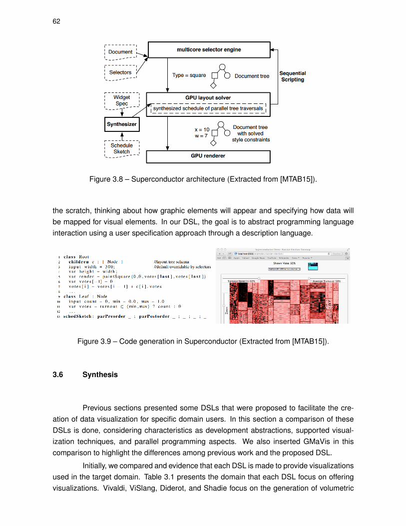
62

Figure 3.8 – Superconductor architecture (Extracted from [MTAB15]).

the scratch, thinking about how graphic elements will appear and specifying how data willbe mapped for visual elements. In our DSL, the goal is to abstract programming languageinteraction using a user specification approach through a description language.

Figure 3.9 – Code generation in Superconductor (Extracted from [MTAB15]).

3.6 Synthesis

Previous sections presented some DSLs that were proposed to facilitate the cre-ation of data visualization for specific domain users. In this section a comparison of theseDSLs is done, considering characteristics as development abstractions, supported visual-ization techniques, and parallel programming aspects. We also inserted GMaVis in thiscomparison to highlight the differences among previous work and the proposed DSL.

Initially, we compared and evidence that each DSL is made to provide visualizationsused in the target domain. Table 3.1 presents the domain that each DSL focus on offeringvisualizations. Vivaldi, ViSlang, Diderot, and Shadie focus on the generation of volumetric

63

visualizations and do not provide geospatial data visualization maps creation. Supercon-ductor [MTAB15] offers a set of generic big data visualization features. It is not designedfor a specific visualization type. Also, it allows the user to personalize the visualization bychanging visual elements. Compared to our work, Superconductor is more robust. However,users have to build their visualizations from scratch interacting with low-level programming,while we abstract programming language interaction using a user specification approach.Thus, analyzing the domain and the supported visualizations, these DSLs have differentapproaches from what we propose in GMaVis.

Table 3.1 – Domain of each DSL.DSL Domain

Vivaldi [CCQ+er] Scientific/Volume VisualizationViSlang [RBGH14] Scientific/Volume VisualizationDiderot [CKR+12] Image Analysis and Medical VisualizationShadie [HWCP15] Medical Visualization

Superconductor [MTAB15] General Interactive VisualizationGMaVis [LGMF15] Geospatial Data Visualization Maps

A common goal in these DSLs is offering high-level interfaces for abstracting pro-gramming complexities. Most of these complexities are about low-level specifications, ren-dering, and parallel processing. Moreover, if we analyze complexity abstractions consideringthe phases of visualization creation described in Section 2.2 we can highlight that the DSLsabstract only complexities from visual mappings and view transformation phases. Table 3.6presents the phases that each DSL abstracts.

Table 3.2 – Complexities abstraction in each visualization creation phase.DSL Data Pre-processing Data to Visual Mappings View Transformations

Vivaldi [CCQ+er] X XViSlang [RBGH14] X XDiderot [CKR+12] X XShadie [HWCP15] X X

Superconductor [MTAB15] X XGMaVis [LGMF15] X X X

Through this comparison, it is possible to verify that only GMaVis abstracts com-plexities from data pre-processing phase. This phase includes a great deal of work requiredto create a visualization, which involves handling data to select, classify and format it. Ifthese data are generated using different formats than those expected by the visualizationtool/library, users will have additional work to format. Some DSLs were built as internal DSL,which means that users can use the general purpose language to deal with data before in-serting it in the mechanisms offered by the DSL. However, users will need to create codeto deal with this data. This phase becomes even harder if users are dealing with huge datafiles. For example, when a domain user needs to generate a visualization of data stored ina file with 30 GBytes. If the computer used have only 4 GBytes of memory, this user willhave to split this file to read and process. Furthermore, if the file has 500GB or 1TB, it can

64

become very slow, often requiring parallel processing to speed it up. Therefore, it impliesmore effort for development.

With data production increasing exponentially, it is easy to achieve Gigabytes orTerabytes of data. Thus, GMaVis offers complexity abstraction in the data pre-processingphase, through the specification of filters and classification of data. Also, parallel program-ming is completely abstracted from users. Moreover, it abstracts complexities in data to vi-sual mappings and view transformations, since users will simply specify a few details aboutthe data visualization map using a descriptive language.

The DSLs presented in this work apply parallel processing to speed up processing.Some DSLs apply parallel programming in the rendering of volumes and for generatingvisualizations. Others use this in interaction, through the use of GPU processing. In ourcase, GMaVis provides parallel processing in the data pre-processing phase, for filtering,classifying and selecting data. Table 3.3 compares the application of parallel programmingamong the DSLs.

Table 3.3 – Parallel processing in each visualization creation phase.DSL Data Pre-processing Data to Visual Mappings View Transformations

Vivaldi [CCQ+er] X XViSlang [RBGH14] X XDiderot [CKR+12] X XShadie [HWCP15] X X

Superconductor [MTAB15] X XGMaVis [LGMF15] X

We can highlight that almost DSLs apply parallel processing in data to visual map-pings and view transformations phases. Also, these DSLs do not apply parallel processingin data pre-processing phase. However, GMaVis applies parallel processing in the data pre-processing phase but does not apply in the data to visual mappings and view transforma-tions phases. It is because GMaVis visualizations do not require high processing to createand display visualization. The costlier processing is the data pre-processing phase, whichincludes loading, parsing, classifying, filtering, selecting and formatting data. Also, Vivaldi,ViSlang, Diderot, Shadie, and Superconductor provide visualizations in 3D and volumetricimages that require high processing to enable both interaction and visualization creation.

65

4. GMAVIS: A DSL FOR GEOSPATIAL DATA VISUALIZATION MAPS

During background studies, we did not found a tool that provides data process-ing and easy ways for domain users to create a visualization. For these users, it becamea hard task since some of them may have a low-level knowledge in computer program-ming [WWA15, ZCL13]. For example, to create a data visualization, users have to deal withdata processing, analysis, and visualization algorithms/technologies. Some domain usersdo not have this knowledge about computer programming and may have a hard time gener-ating a simple visualization. Also, users that need to generate a simple map with markersmay know at least HTML and JavaScript. Additionally, this user will need to learn how to usea library, like Google Maps API or OpenLayers. If this user is handling a huge dataset, thistask becomes harder since a third software or tool to process, select and filter this data willbe required.

Therefore, we decided to develop GMaVis, an external DSL that provides an auto-matic generation of data visualizations for large-scale geospatial data. This DSL provides ahigh-level interface through a description language that can receive additional visualizationsin future. Since it abstracts complexities from computer programming issues, such as func-tions, variables, methods and web development issues, it is more accessible for users withlow-level knowledge of computer programming to create data visualizations and analyzesdata.

The first section of this chapter introduces GMaVis, presenting its main advantages,characteristics, context, environment, and explaining how it interacts with users. Also, thissection briefly presents the compiler modules. Section 4.2 then formalizes GMaVis’ grammarand language, explaining the possible declarations, blocks and values. Finally, Sections 4.3and 4.4 briefly describe the function and objectives of GMaVis’ internal modules.

4.1 The Proposed DSL

To facilitate the creation of visualizations for large-scale geospatial data, we pro-pose GMaVis, an external DSL to provide a high-level specification language [LGMF15].The goal is to be as close as possible to the domain vocabulary, supporting a suitable andfriendly language syntax. It has a description language with a high level of abstraction thatenables users to express filter, classification, data format, and visualization details specifi-cation. This language has limited expressiveness which makes easy for the user to learnthis.

This DSL abstracts many programming and data processing aspects. Instead ofcreating a visualization using general purpose languages that require some computer pro-

66

gramming knowledge, users can specify the desired visualization and how the data must beprocessed in only a few lines of code. The DSL performs all data parsing, processing, andclassification, generating the visualization. Moreover, this DSL abstracts the transformationphase, as explained in Chapter 3 and as shown in Figure 4.1 where it is possible to seethe scope that traditional visualization tools abstract from users. Figure 4.1(a) demonstratestraditional visualization tools that simply abstract the visualization generation phase fromusers. Data pre-processing is not included in the scope since features are not provided toimprove users experience in this aspect. The proposed DSL, illustrated in Figure 4.1(b) ab-stracts the whole pipeline for creating a visualization because it offers data pre-processingmechanisms. Therefore, users do not have to preprocess data manually or use externaltools.

Figure 4.1 – Data visualization creation comparison.

Users of this DSL instead of other tools and libraries as Google Maps API, Leafletand OpenLayers will have some advantages. First they will not have to know programmingaspects like functions, variables, methods and any other web development issue. Second,the user will have a data processing that empowers data filtering, cleaning, and classifica-tion automatically. This DSL provides the same operations when working with huge files,because it offers an optimized file loading in memory that allows one to open files biggerthan the RAM memory available in the equipment. The third advantage is that this DSLis not linked with a host language, and its interface is extremely close to the user domain.Furthermore, the parallel programming in this DSL is completly abstracted. Users will havea parallel data preprocessor without being required to implement any parallel code. This ispossible because we use another DSL to generate parallel code.

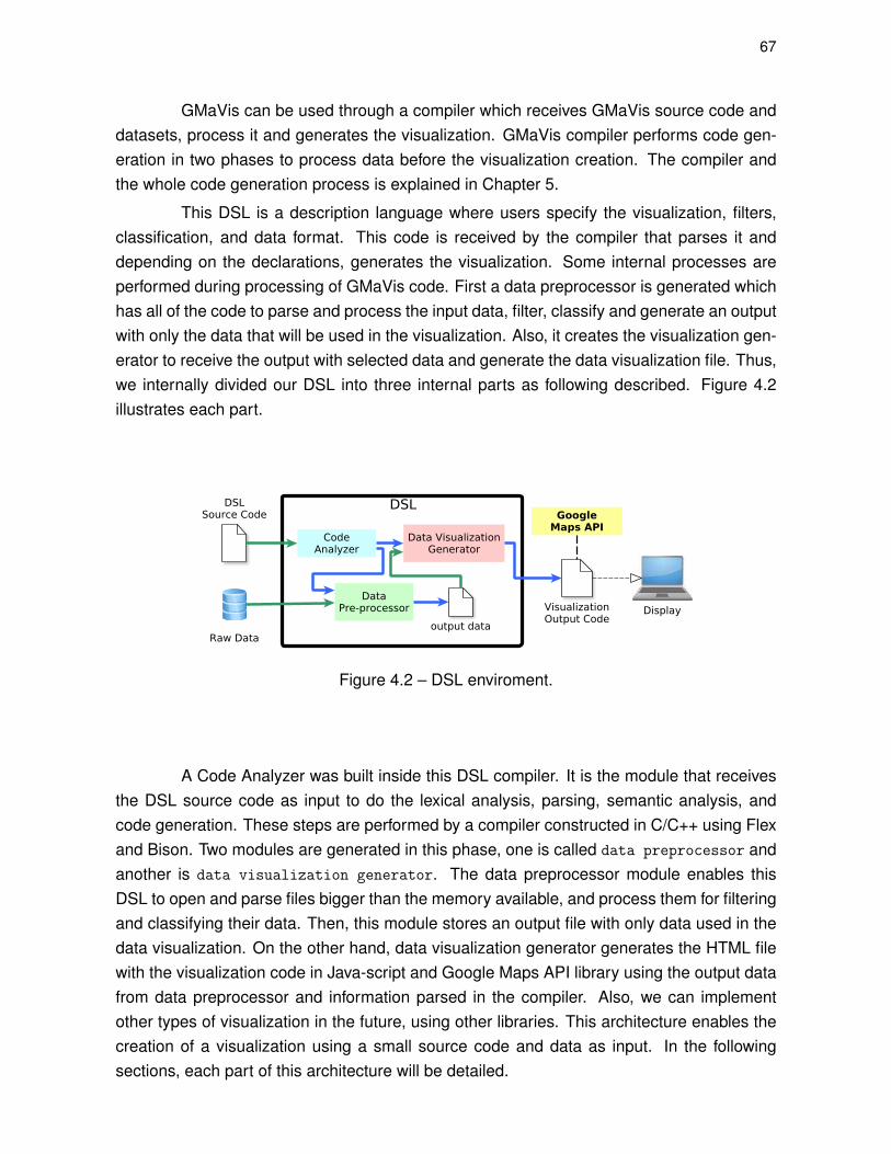
67

GMaVis can be used through a compiler which receives GMaVis source code anddatasets, process it and generates the visualization. GMaVis compiler performs code gen-eration in two phases to process data before the visualization creation. The compiler andthe whole code generation process is explained in Chapter 5.

This DSL is a description language where users specify the visualization, filters,classification, and data format. This code is received by the compiler that parses it anddepending on the declarations, generates the visualization. Some internal processes areperformed during processing of GMaVis code. First a data preprocessor is generated whichhas all of the code to parse and process the input data, filter, classify and generate an outputwith only the data that will be used in the visualization. Also, it creates the visualization gen-erator to receive the output with selected data and generate the data visualization file. Thus,we internally divided our DSL into three internal parts as following described. Figure 4.2illustrates each part.

DSL

Figure 4.2 – DSL enviroment.

A Code Analyzer was built inside this DSL compiler. It is the module that receivesthe DSL source code as input to do the lexical analysis, parsing, semantic analysis, andcode generation. These steps are performed by a compiler constructed in C/C++ using Flexand Bison. Two modules are generated in this phase, one is called data preprocessor andanother is data visualization generator. The data preprocessor module enables thisDSL to open and parse files bigger than the memory available, and process them for filteringand classifying their data. Then, this module stores an output file with only data used in thedata visualization. On the other hand, data visualization generator generates the HTML filewith the visualization code in Java-script and Google Maps API library using the output datafrom data preprocessor and information parsed in the compiler. Also, we can implementother types of visualization in the future, using other libraries. This architecture enables thecreation of a visualization using a small source code and data as input. In the followingsections, each part of this architecture will be detailed.

68

4.2 Interface

This DSL contributes by providing a high-level interface for processing, filtering,classifying data and creating data visualization maps. It enables the creation of a data visu-alization using only a few lines of code. We created GMaVis with a description language forsimplifying the implementation of a new data visualization. It has its own grammar, thus, wecan classify it as an external DSL. This decision was made because an external languagesimplifies the use since we have the freedom to create an interface similar to natural lan-guage. Being an external DSL, it only enables the creation of code to specify a supporteddata visualizations, since it has a limited expressiveness. However, it is easy to learn anduse GMaVis, since it has a short grammar, close to the domain vocabulary. Therefore, theuser will not need to worry about other characteristics of host languages, such as functions,variables, and low-level programming, as in internal DSLs or general purpose languages.

This DSL language consists of blocks, declarations, properties, and values. A blockis defined as a keyword followed by an ’{’ character, a list of declarations and a ’}’ character.A declaration has a property and value. All GMaVis properties are formed by keywords anda colon (’:’) character. Finally, values can be literals (strings, characters, integer or floatnumbers), logical expressions, fields specifications, or keywords. Each declaration acceptssome specific values that are checked during compilation.

GMaVis has three main elements specified globally in the source code. The firstelement consists of a visualization declaration which specifies the type of data visualizationto be created. The second element is a settings block with declarations about visualizationdetails such as latitude/longitude fields, size, and title. Finally, a data block with declarationsused in data processing such as filters, classification, data structure and delimiters must bedeclared.

The goal is to boost this DSL with other types of data visualization. It was built usinggeneralizations for adding new visualization techniques in the future. The specification of thecode starts with a visualization declaration informing the visualization type name as a value.With this, we can implement other types of data visualization in the future, and users canchange the type of visualization easily by just changing a few lines of code.

The EBNF for this grammar can be found in appendix B. Also, details about theparsing performed and compilation is explained in Chapter 5.

4.2.1 Keywords

This DSL has some reserved words that are recognized in the lexical analysis andgive meaning to the grammar. They must be used in the right place to effectively express

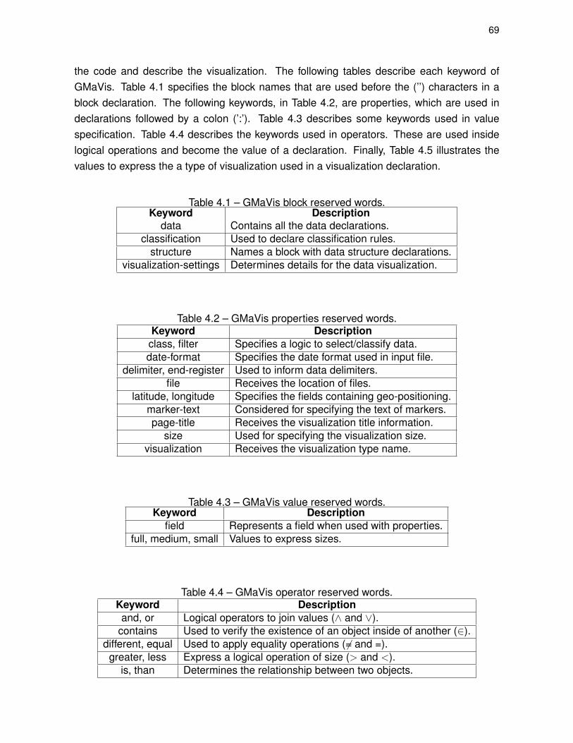
69

the code and describe the visualization. The following tables describe each keyword ofGMaVis. Table 4.1 specifies the block names that are used before the (’’) characters in ablock declaration. The following keywords, in Table 4.2, are properties, which are used indeclarations followed by a colon (’:’). Table 4.3 describes some keywords used in valuespecification. Table 4.4 describes the keywords used in operators. These are used insidelogical operations and become the value of a declaration. Finally, Table 4.5 illustrates thevalues to express the a type of visualization used in a visualization declaration.

Table 4.1 – GMaVis block reserved words.Keyword Description

data Contains all the data declarations.classification Used to declare classification rules.

structure Names a block with data structure declarations.visualization-settings Determines details for the data visualization.

Table 4.2 – GMaVis properties reserved words.Keyword Descriptionclass, filter Specifies a logic to select/classify data.date-format Specifies the date format used in input file.

delimiter, end-register Used to inform data delimiters.file Receives the location of files.

latitude, longitude Specifies the fields containing geo-positioning.marker-text Considered for specifying the text of markers.page-title Receives the visualization title information.

size Used for specifying the visualization size.visualization Receives the visualization type name.

Table 4.3 – GMaVis value reserved words.Keyword Description

field Represents a field when used with properties.full, medium, small Values to express sizes.

Table 4.4 – GMaVis operator reserved words.Keyword Descriptionand, or Logical operators to join values (∧ and ∨).

contains Used to verify the existence of an object inside of another (∈).different, equal Used to apply equality operations (�= and =).

greater, less Express a logical operation of size (> and <).is, than Determines the relationship between two objects.

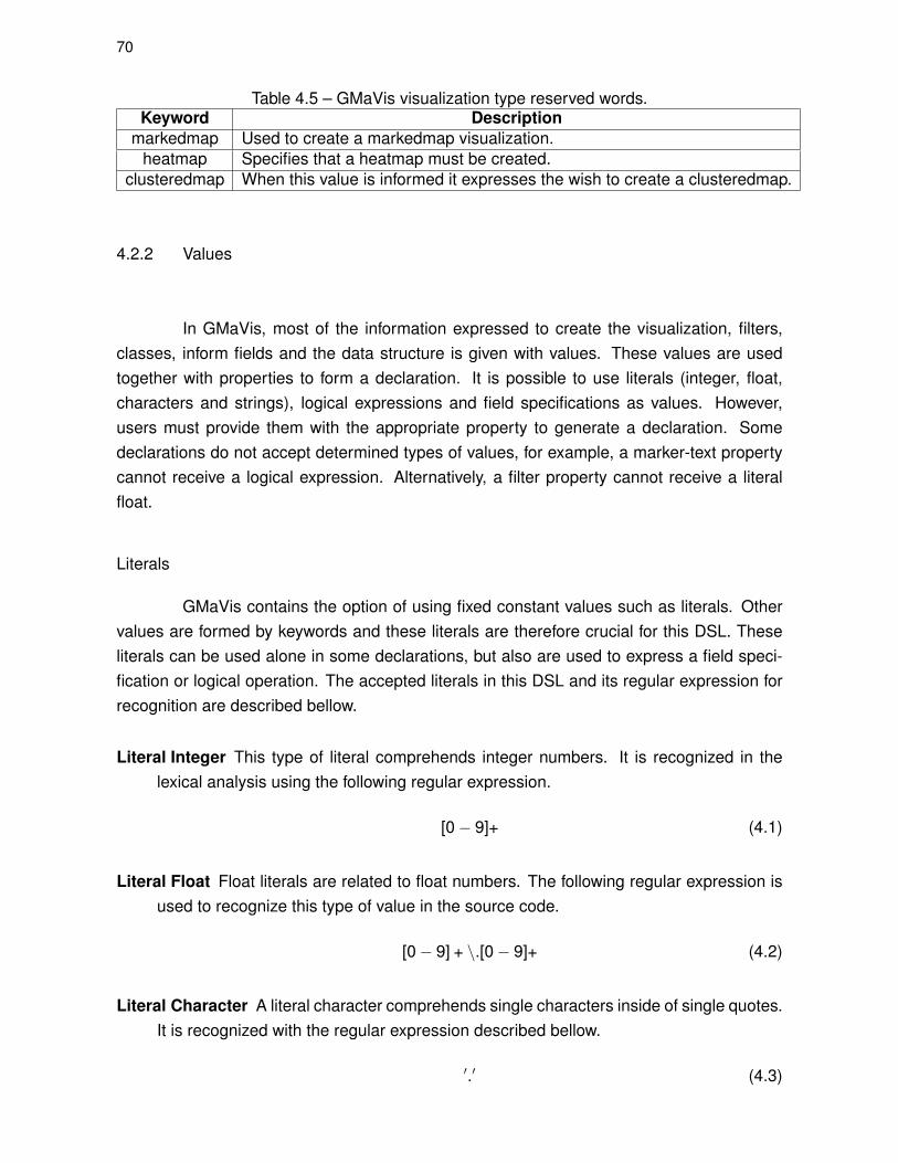
70

Table 4.5 – GMaVis visualization type reserved words.Keyword Description

markedmap Used to create a markedmap visualization.heatmap Specifies that a heatmap must be created.

clusteredmap When this value is informed it expresses the wish to create a clusteredmap.

4.2.2 Values

In GMaVis, most of the information expressed to create the visualization, filters,classes, inform fields and the data structure is given with values. These values are usedtogether with properties to form a declaration. It is possible to use literals (integer, float,characters and strings), logical expressions and field specifications as values. However,users must provide them with the appropriate property to generate a declaration. Somedeclarations do not accept determined types of values, for example, a marker-text propertycannot receive a logical expression. Alternatively, a filter property cannot receive a literalfloat.

Literals

GMaVis contains the option of using fixed constant values such as literals. Othervalues are formed by keywords and these literals are therefore crucial for this DSL. Theseliterals can be used alone in some declarations, but also are used to express a field speci-fication or logical operation. The accepted literals in this DSL and its regular expression forrecognition are described bellow.

Literal Integer This type of literal comprehends integer numbers. It is recognized in thelexical analysis using the following regular expression.

[0 − 9]+ (4.1)

Literal Float Float literals are related to float numbers. The following regular expression isused to recognize this type of value in the source code.

[0 − 9] + \.[0 − 9]+ (4.2)

Literal Character A literal character comprehends single characters inside of single quotes.It is recognized with the regular expression described bellow.

�.� (4.3)

71

Literal String This represents a combined set of characters, escape sequences, ponctua-tion and any characters. It is recognized with the following regular expression.

\��(\ \ .|[∧\\��])∗\�� (4.4)

This DSL does not require the use of other literal types, such as booleans, to ex-press the description of supported visualization types. However, it is possible to implementother literal types in the future if a novel visualization type were to require this.

Logical Expressions

Logical expressions were required in this DSL for specifying filters and classes ofdata. Logical expressions have one or more logical operations. These logical operationscan be combined using OR or AND operators. GMaVis has eight logical operations imple-mented that can be combined to express a logical expression in a filter or class declaration.Figure 4.3 illustrates the possible logical operations in GMaVis using x for fields positions,and y and z to express literal values. This also demonstrates the possibility of combiningoperators through a link with AND and OR operators.

Figure 4.3 – Logical operators to filter and classify.

The structure of a logical operation has a field specification followed by a logicaloperator. Most operators receives a string value or a field representation. Moreover, theoperator is between has a structure that includes an AND operator to express that the fieldvalue must be among the values specified before and after it.

The main objective when using these logical expressions is to express a conditionto be applied to data registers. If the logical expression is determined to be true when appliedto a data register, it will be used. Otherwise, it will not. Therefore, logical expressions canbe used in filtering to select registers or in classes to input registers into a class.

72

Field Specification

The specification of fields enables the data preprocessor to locate data inside thedataset for manipulation. Considering that most raw datasets have a structure with delimitercharacters to separate data in an organized way it is possible to specify each field usingliteral integers. Figure 4.4 illustrates the identification of a field number in a simple dataset.

Figure 4.4 – Field value in dataset.

In the grammar, a field specification has a field keyword followed by a literal in-teger. These specifications are used in many declarations, such as marker-text, latitudeand longitude, filters, and classes. These fields are recognized during data pre-processingthrough the data split using the delimiters specified in user source code.

Size Specification

Size specifications are values that use the keywords small, medium and full toexpress a size. They are used in size declaration to specify the size for a visualization in aHTML page. For example, if a full value is specified for the visualization, this will occupythe whole page. Otherwise, other values will adjust the visualization for other sizes. If a userwith more experience intends to modify the HTML page to insert some text or even insertthe visualization in a website, they can use small or medium values to occupy 50% or 80%of the page. Moreover, if the user is not satisfied with the size and prefers to adjust it foranother size, the width and height values can be changed in the generated HTML file.

Visualization Type Specification

GMaVis offers the creation of three different visualization types: markedmap, clus-teredmap, and heatmap. To specify in the source code which type of visualization mustbe created, a visualization type specification is used. Table 4.5 describe the three possiblekeywords allowed to express a visualization type.

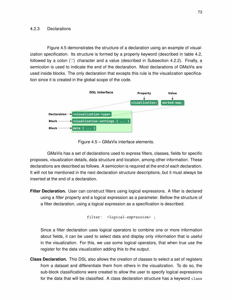
73

4.2.3 Declarations

Figure 4.5 demonstrates the structure of a declaration using an example of visual-ization specification. Its structure is formed by a property keyword (described in table 4.2,followed by a colon (’:’) character and a value (described in Subsection 4.2.2). Finally, asemicolon is used to indicate the end of the declaration. Most declarations of GMaVis areused inside blocks. The only declaration that excepts this rule is the visualization specifica-tion since it is created in the global scope of the code.

Figure 4.5 – GMaVis interface elements.

GMaVis has a set of declarations used to express filters, classes, fields for specificproposes, visualization details, data structure and location, among other information. Thesedeclarations are described as follows. A semicolon is required at the end of each declaration.It will not be mentioned in the next declaration structure descriptions, but it must always beinserted at the end of a declaration.

Filter Declaration. User can construct filters using logical expressions. A filter is declaredusing a filter property and a logical expression as a parameter. Bellow the structure ofa filter declaration, using a logical expression as a specification is described.

filter: <logical-expression> ;

Since a filter declaration uses logical operators to combine one or more informationabout fields, it can be used to select data and display only information that is usefulin the visualization. For this, we use some logical operators, that when true use theregister for the data visualization adding this to the output.

Class Declaration. This DSL also allows the creation of classes to select a set of registersfrom a dataset and differentiate them from others in the visualization. To do so, thesub-block classifications were created to allow the user to specify logical expressionsfor the data that will be classified. A class declaration structure has a keyword class

74

followed by a colon (’:’) character and a logical expression, equal to the one used infilters. This logical expression will be applied in all the dataset registers. When it isfound true, the register will be inserted in the class.

class : <logical-expression> ;

Users can also inform an alias for each class. In this case, a legend using the classesnames will be generated.

Latitude/Longitude Declaration Geospatial data visualizations require an important typeof data that represents position. GMaVis has two declarations to receive this informa-tion through of a value with field specification. Both latitude and longitude declarationsare required to generate the visualization. Without this information, it is not possibleto insert data in a map visualization. The structure of both is the same, except for thekeyword. It is a keyword, latitude or longitude, a colon (’:’) character followed by afield specification value.

latitude : <field-specification> ;

longitude : <field-specification> ;

These declarations enable the data preprocessor to insert latitude and longitude infor-mation directly in the output code for selected data.

File declaration File declarations are used to express the path to a file with data. It ispossible to have an unlimited quantity of files in a source code since a dataset can besplit into a set of files with data. This declaration structure begins with a keyword file,followed by a colon (’:’) character and a literal string. In this literal string, users mayinform the path to the file that will be processed. The structure is described below.

file : <literal-string> ;

Delimiter/End-register Declaration Users can specify the characters used as delimiter inthe data fields through the delimiter declaration. They can also inform the characterused to mark the end of a register. For example, in a CSV (Comma Separated Values)file, the delimiter will be the comma (’,’) and the end register will be a new line character.

delimiter : <literal-character> ;

end-register : <literal-character> ;

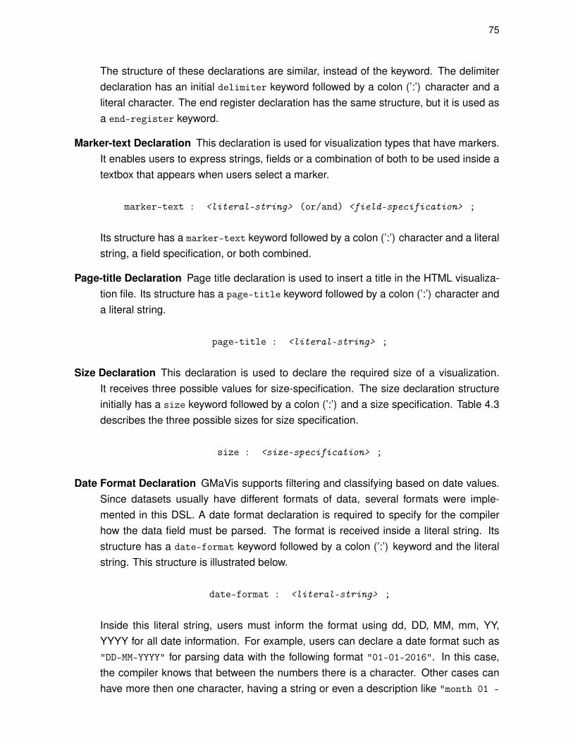
75

The structure of these declarations are similar, instead of the keyword. The delimiterdeclaration has an initial delimiter keyword followed by a colon (’:’) character and aliteral character. The end register declaration has the same structure, but it is used asa end-register keyword.

Marker-text Declaration This declaration is used for visualization types that have markers.It enables users to express strings, fields or a combination of both to be used inside atextbox that appears when users select a marker.

marker-text : <literal-string> (or/and) <field-specification> ;

Its structure has a marker-text keyword followed by a colon (’:’) character and a literalstring, a field specification, or both combined.

Page-title Declaration Page title declaration is used to insert a title in the HTML visualiza-tion file. Its structure has a page-title keyword followed by a colon (’:’) character anda literal string.

page-title : <literal-string> ;

Size Declaration This declaration is used to declare the required size of a visualization.It receives three possible values for size-specification. The size declaration structureinitially has a size keyword followed by a colon (’:’) and a size specification. Table 4.3describes the three possible sizes for size specification.

size : <size-specification> ;

Date Format Declaration GMaVis supports filtering and classifying based on date values.Since datasets usually have different formats of data, several formats were imple-mented in this DSL. A date format declaration is required to specify for the compilerhow the data field must be parsed. The format is received inside a literal string. Itsstructure has a date-format keyword followed by a colon (’:’) keyword and the literalstring. This structure is illustrated below.

date-format : <literal-string> ;

Inside this literal string, users must inform the format using dd, DD, MM, mm, YY,YYYY for all date information. For example, users can declare a date format such as"DD-MM-YYYY" for parsing data with the following format "01-01-2016". In this case,the compiler knows that between the numbers there is a character. Other cases canhave more then one character, having a string or even a description like "month 01 -

76

day 01 - year 2016". This case would require a string like "month MM - day DD -

year YYYY". Thus, this compiler enables the parsing of the basic and most commonlyused date formats, even if inside a description1.

Visualization Declaration One of the most important declarations in GMaVis is the visual-ization declaration. This specifies the type of visualization that will be created.

visualization : <visualization-type-specification> ;

It is declared in the global scope of the code, and its structure has a visualization

keyword, followed by a colon (’:’) and a visualization type specification. Current visual-ization types that GMaVis support are described in Table 4.5.

4.2.4 Blocks

GMaVis organizes declarations in blocks. Each block contains declarations that areformed by property and value. GMaVis has four different blocks: data block, classificationblock, structure block and settings block. The structure of a block is a keyword followed bya left brace character, a declaration sequence and finally a right brace character. Figure 4.6uses a settings block to illustrate the structure

Figure 4.6 – GMaVis settings block example.

In global scope, GMaVis receives two blocks, one for data and another for settingsome details about the visualization. Also, two or more subblocks inside of a data blockshould be used to express classification and structure. Each block and accepted declara-tions are described bellow.

Block Data Data block has declarations related to data processing. It contains declarationswith information about input data and how it will be loaded and processed by the datapreprocessor. This block is divided in four elements: file declarations, a structure block,a filter declaration, and a classification block.

1Currently, GMaVis does not include or consider processing date formats with a text description for monthsor numbers, such as January, February, March, etc. It is planed for future work.

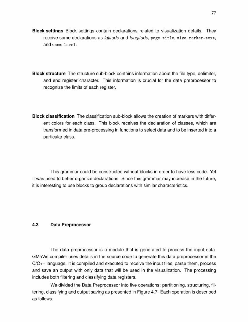
77

Block settings Block settings contain declarations related to visualization details. Theyreceive some declarations as latitude and longitude, page title, size, marker-text,and zoom level.

Block structure The structure sub-block contains information about the file type, delimiter,and end register character. This information is crucial for the data preprocessor torecognize the limits of each register.

Block classification The classification sub-block allows the creation of markers with differ-ent colors for each class. This block receives the declaration of classes, which aretransformed in data pre-processing in functions to select data and to be inserted into aparticular class.

This grammar could be constructed without blocks in order to have less code. YetIt was used to better organize declarations. Since this grammar may increase in the future,it is interesting to use blocks to group declarations with similar characteristics.

4.3 Data Preprocessor

The data preprocessor is a module that is generated to process the input data.GMaVis compiler uses details in the source code to generate this data preprocessor in theC/C++ language. It is compiled and executed to receive the input files, parse them, processand save an output with only data that will be used in the visualization. The processingincludes both filtering and classifying data registers.

We divided the Data Preprocessor into five operations: partitioning, structuring, fil-tering, classifying and output saving as presented in Figure 4.7. Each operation is describedas follows.

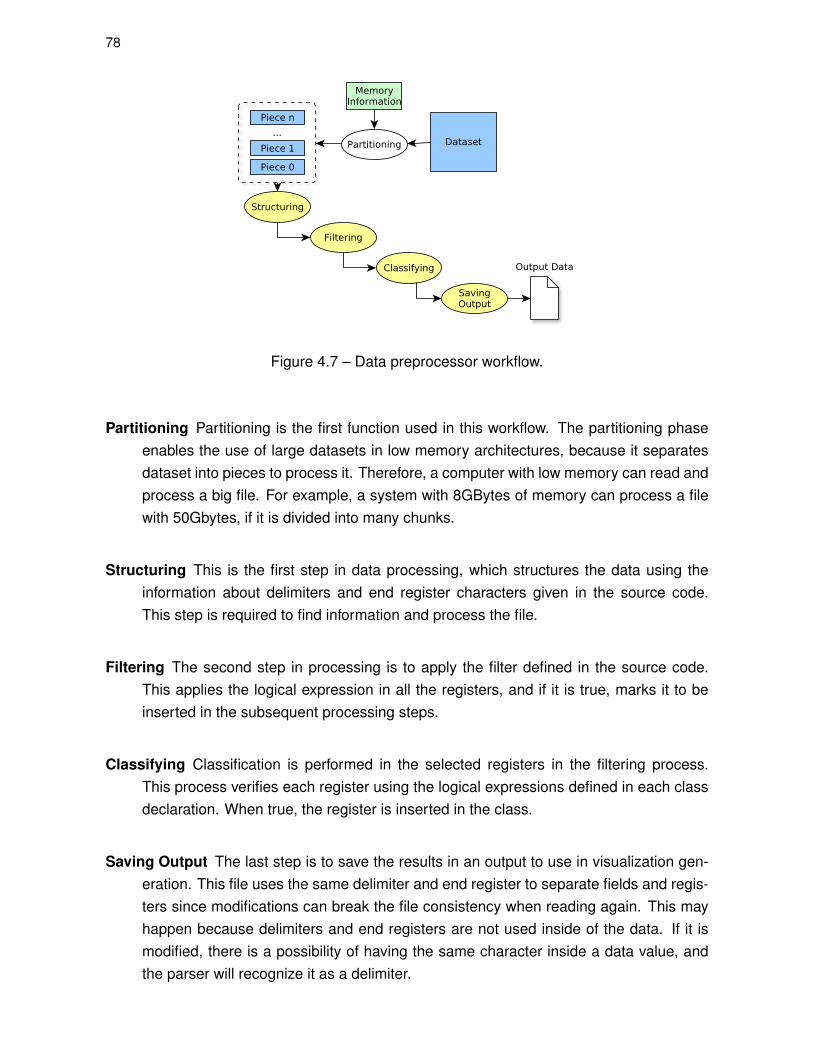
78

Figure 4.7 – Data preprocessor workflow.

Partitioning Partitioning is the first function used in this workflow. The partitioning phaseenables the use of large datasets in low memory architectures, because it separatesdataset into pieces to process it. Therefore, a computer with low memory can read andprocess a big file. For example, a system with 8GBytes of memory can process a filewith 50Gbytes, if it is divided into many chunks.

Structuring This is the first step in data processing, which structures the data using theinformation about delimiters and end register characters given in the source code.This step is required to find information and process the file.

Filtering The second step in processing is to apply the filter defined in the source code.This applies the logical expression in all the registers, and if it is true, marks it to beinserted in the subsequent processing steps.

Classifying Classification is performed in the selected registers in the filtering process.This process verifies each register using the logical expressions defined in each classdeclaration. When true, the register is inserted in the class.

Saving Output The last step is to save the results in an output to use in visualization gen-eration. This file uses the same delimiter and end register to separate fields and regis-ters since modifications can break the file consistency when reading again. This mayhappen because delimiters and end registers are not used inside of the data. If it ismodified, there is a possibility of having the same character inside a data value, andthe parser will recognize it as a delimiter.

79

4.3.1 Data Processing Algorithm

Processing a huge quantity of data can be costly. Thus, it is important that thesoftware that performs this operation uses smart search and selection of registers. Also,memory usage is a critical factor in this process. If an algorithm requires data replicationto perform operations, it will require more cycles of processing pieces of data to finish theexecution.

Considering this context and with the objective of implementing and optimizing thealgorithm for processing data, we did a study on search algorithms [CL11] to choose anoptimal one to perform the register selection. This study is based on the complexity time ofeach algorithm expressed using the Big O notation [Knu76, DSR11, Hil04]. Three searchalgorithms were analyzed: Linear Search, Binary Tree, and Interpolation Search.

For the comparison, we used the time and space complexity. As these algorithmswould be used to process huge quantities of data, we considered the worst case to comparethem. Also, space complexity was considered to compare these algorithms because thememory space used is an important issue to consider. Obviously, on the actual multi-corecomputer architectures, this may present a memory problem. Thus, for this evaluation wesought an algorithm that presents a minimum O(n) for worst time-space, maintaining thesame quantity of data.

Table 4.6 presents the time complexity of each algorithm. Also, it exposes the limi-tations in respect to sorted and unsorted data. We highlight that the linear search algorithmhas the largest complexity time because this verifies all the elements of the array during thesearch. On the other hand, this algorithm does not require a sorted array. Moreover, binarysearch and interpolation search algorithms present lower complexity times, they requires asorted array to find one or a set of registers.

Table 4.6 – Time complexity of search algorithms.Algorithm Name Time Complexity Limitation

Linear Seach O(n) No LimitationBinary Search O(n log n) Sorted Dataset

Interpolation Search O(log log n) Sorted Dataset

Through this analysis, we can highlight that, for ordered arrays, an interpolationsearch algorithm is the best alternative because this has a lower time complexity. Other-wise, for disordered arrays, the linear search is more convenient because this does notneed the use of a sort algorithm to organize registers. To certify if it would be possible tocombine an interpolation or binary search algorithm with a sorting algorithm to obtain betterresults in unsorted arrays, in Table 4.7 we analyze these algorithms combining them withsome sorting algorithms. Considering LS as Linear search, BS as a Binary Search and IS

80

as an Interpolation Search. In this comparison, we used the sum of both search and sort al-gorithms. Therefore, considering that when combining two O values the greater is the result,we used the greater value to compare each combination with the Linear Search algorithm.

Table 4.7 – Search algorithm comparison considering sorting.

AlgorithmsTime

Complexity(Worst)

TimeComplexity

(Total)

SpaceComplexity

(Total)LS O(n) O(n) O(n)

BS+Merge Sort O(log n)+O(n log n) O(n log n) O(n)BS+Quicksort O(log n) + O(n log n) O(n log n) O(n)BS+Heapsort O(log n)+O(n log n) O(n log n) O(1)

BS+Selection Sort O(log n)+O(n2) O(n2) O(n)BS+Bubble Sort O(log n)+O(n2) O(n2) O(1)BS+Gnome Sort O(log n)+O(n2) O(n2) O(1)

BS+Insertion Sort O(log n)+O(n2) O(n2) O(n)BS+Radix Sort O(log n)+O(kn) O(kn) O(k + n)IS+Merge Sort O(log log n)+O(n log n) O(n log n) O(n)IS+Quicksort O(log log n)+O(n log n) O(n log n) O(n)IS+Heapsort O(log log n)+O(n log n) O(n log n) O(1)

IS+Selection Sort O(log log n)+O(n2) O(n2) O(n)IS+Bubble Sort O(log log n)+O(n2) O(n2) O(1)IS+Gnome Sort O(log log n)+O(n2) O(n2) O(1)

IS+Insertion Sort O(log log n)+O(n2) O(n2) O(n)IS+Radix Sort O(log log n)+O(kn) O(kn) O(k + n)

As verified in Table 4.7, the time complexity of binary and interpolation search algo-rithms are increased with sorting operations. The implementation of a binary or interpolationsearch is more complex than a linear search algorithm since it needs the development ofa sorting algorithm. As analyzed, most these algorithms will be performed using unsorteddatasets if applied in our data preprocessor. Considering the information presented, wecreated the processing functions based on a linear search algorithm, performing filters andclassifications in the whole dataset.

4.4 Visualization Generator

The last step in generating the visualization in GMaVis is performed in the visual-ization generator. This module receives the output data from the data preprocessor and theinformation from the source code. Then, the visualization generator produces data visual-ization code in HTML according to the specifications declared in the DSL source code. Theoutput file of this module is an HTML file with visualization.

81

The visualization generator receives information from the code analyzer about de-tails specified in the setting block. This is used in code generation to print HTML andJavascript code in the file, combined with data preprocessor output data. Finally, it cre-ates an output file containing the required code to display the visualization map with theGoogle Maps API call, information about the title, sizes, markers, legends, and the data tobe presented.

Our DSL does not generate the visual elements of the data visualization fromscratch. To facilitate code generation, libraries such as Google Maps API are used in theHTML to generated code. This library was chosen to convert data to visual mappings,because it requires a short code for a simple code generation and provides a high-level in-terface for manipulating map details and inserting data. It also allows the implementationof other types of visualizations in the future without changing either the DSL architecture oroutput of the data preprocessor.

The HTML file with the visualization is generated by simply printing strings withcommon code directly in a file. However, there are pieces of code that are modified depend-ing the visualization, data, specification details or other issues that require special attention.The type of code required to be generated in that specific part is verified through conditionsstatements. More details about the visualization generator, code generation, its internalfunctions, iteration with other modules, generation of HTML file and other internal details areexplained in Chapter 5.

4.5 Use Cases

For better understanding of GMaVis grammar some use cases that demonstratessix applications (2 for each visualization type) using the GMaVis features will be presentedin this section. This starts with Subsection 4.5.1 that exposes the three datasets employedin this applications. Subsection 4.5.2 presents their descriptions, codes and output images.These applications also were used in the GMaVis evaluations presented in Chapter 6.

4.5.1 Datasets

In these use cases, real-world data was used. Among the six developed applica-tions, each dataset is used for two applications. Thus, we used three datasets for theseexperiments. These datasets are described below.

YFCC100M In the first dataset, we used YFCC100M [TSF+15], provided by Yahoo Labs.The YFCC100M dataset has about 54GB of data, divided into ten files. This is a public

82

multimedia data set with 99.3 million images and 0.7 million videos, all from Flickr andunder Creative Commons licensing.

Traffic Accidents We also used a dataset from DataPoa2 with traffic accident data in thecity of Porto Alegre,Brazil that contains information about the type of accidents, vehi-cles, date and time, level and location. It has 39 fields, including latitude and longitude,and about 20.937 registers of accidents between 01-01-2013 and 12-31-2013.

Airports A dataset obtained in OpenFlights3 that contains all the airports in the world wasused, with information about latitude and longitude, city, country and airport code. Ithas 8107 registers with 12 fields with information about the airports.

4.5.2 Sample Applications

In order to demonstrate GMaVis grammar and evaluate the DSL/Compiler, Six vi-sualization applications were created using the datasets presented in subsection 4.5.1. Also,two applications were created for each type of visualization provided in GMaVis (MarkedMap,Heatmap, and Clusteredmap). Each application code and visualization is presented as fol-lows.

Airports in world (clustered map)

In this visualization, a marker is displayed for each airport in the world. It usedclustered map visualization type, which joins markers with less proximity. Thus, it is possibleto identify countries with greater number of airports by clusters with red color. Figure 4.8presents the generated visualization. Listing 4.1 describes the code to create this visualiza-tion using GMaVis.

2Available in: http://www.datapoa.com.br/dataset/acidentes-de-transito3http://openflights.org/data.html

83

1 v i s u a l i z a t i o n : clusteredmap ;2 s e t t i n g s {3 l a t i t u d e : f i e l d 7 ;4 l ong i t ude : f i e l d 8 ;5 marker−t e x t : f i e l d 1 f i e l d 2 f i e l d 3 f i e l d 4 ;6 page− t i t l e : " A i r p o r t s i n World " ;7 s i ze : f u l l ;8 }9 data {

10 f i l e : " vis_codes / a i r p o r t s . dat " ;11 s t r u c t u r e {12 d e l i m i t e r : ’ , ’ ;13 end−r e g i s t e r : newl ine ;14 }15 }

Listing 4.1 – Airports in world (clustered map) code.

Figure 4.8 – Airports in world (clustered map).

Flickr Photos with "Computer" Word as Tag (clustered map)

This visualization also used clustered map to display markers that represent aphoto taken and uploaded to Flickr. This visualization used a filter to select just picturesthat have a tag that contains the word computer. This visualization displayed more occur-rences of pictures with this tag in the United States and England. Figure 4.9 presents thegenerated visualization. Listing 4.2 describes the code for creating this visualization usingGMaVis.

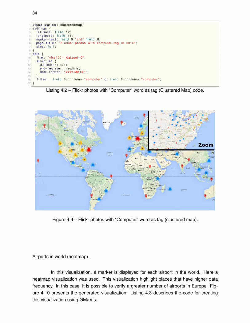
84

1 v i s u a l i z a t i o n : clusteredmap ;2 s e t t i n g s {3 l a t i t u d e : f i e l d 12;4 l ong i t ude : f i e l d 11;5 marker−t e x t : f i e l d 9 " and " f i e l d 8 ;6 page− t i t l e : " F l i c k e r photos wi th computer tag i n 2014 " ;7 s ize : f u l l ;8 }9 data {

10 f i l e : " yfcc100m_dataset−0" ;11 s t r u c t u r e {12 d e l i m i t e r : tab ;13 end−r e g i s t e r : newl ine ;14 date−format : "YYYY−MM−DD" ;15 }16 f i l t e r : f i e l d 8 conta ins " computer " or f i e l d 9 conta ins " computer " ;17 }

Listing 4.2 – Flickr photos with "Computer" word as tag (Clustered Map) code.

Figure 4.9 – Flickr photos with "Computer" word as tag (clustered map).

Airports in world (heatmap).

In this visualization, a marker is displayed for each airport in the world. Here aheatmap visualization was used. This visualization highlight places that have higher datafrequency. In this case, it is possible to verify a greater number of airports in Europe. Fig-ure 4.10 presents the generated visualization. Listing 4.3 describes the code for creatingthis visualization using GMaVis.

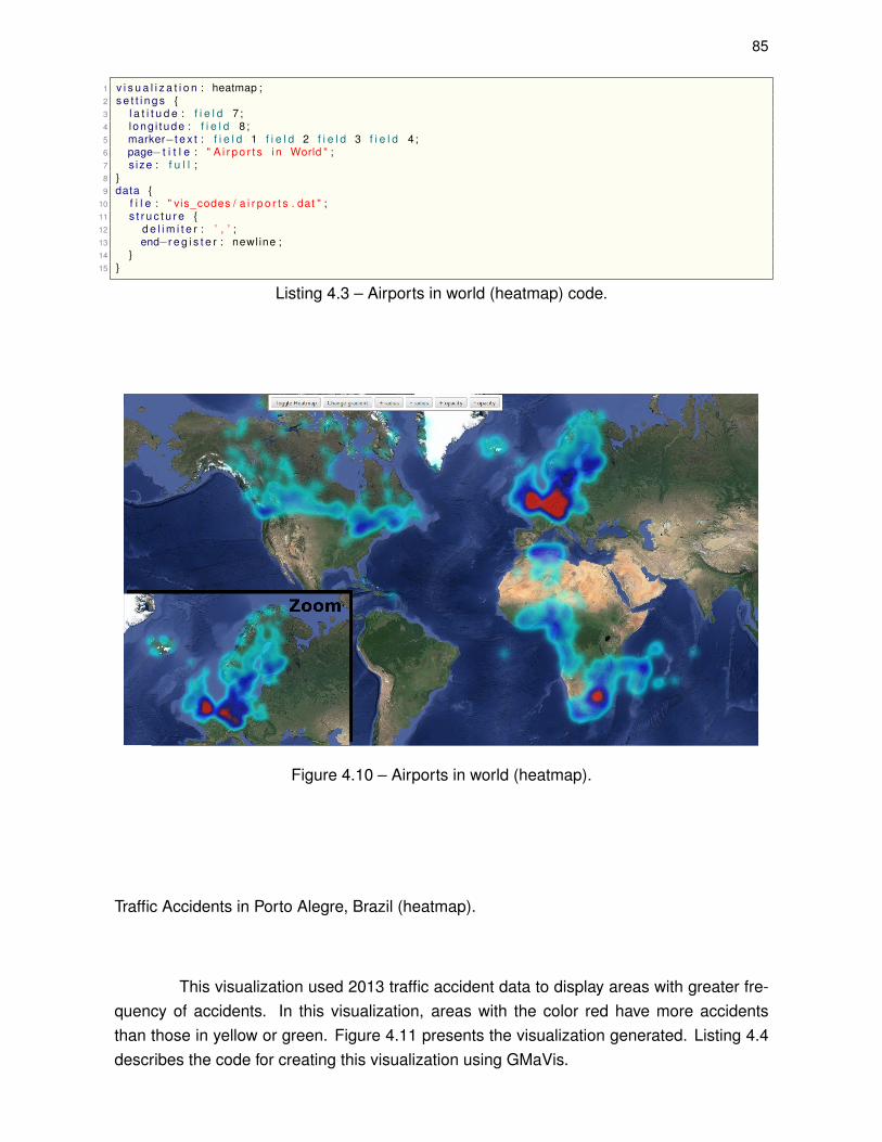
85

1 v i s u a l i z a t i o n : heatmap ;2 s e t t i n g s {3 l a t i t u d e : f i e l d 7 ;4 l ong i t ude : f i e l d 8 ;5 marker−t e x t : f i e l d 1 f i e l d 2 f i e l d 3 f i e l d 4 ;6 page− t i t l e : " A i r p o r t s i n World " ;7 s i ze : f u l l ;8 }9 data {

10 f i l e : " vis_codes / a i r p o r t s . dat " ;11 s t r u c t u r e {12 d e l i m i t e r : ’ , ’ ;13 end−r e g i s t e r : newl ine ;14 }15 }

Listing 4.3 – Airports in world (heatmap) code.

Figure 4.10 – Airports in world (heatmap).

Traffic Accidents in Porto Alegre, Brazil (heatmap).

This visualization used 2013 traffic accident data to display areas with greater fre-quency of accidents. In this visualization, areas with the color red have more accidentsthan those in yellow or green. Figure 4.11 presents the visualization generated. Listing 4.4describes the code for creating this visualization using GMaVis.

86

1 v i s u a l i z a t i o n : heatmap ;2 s e t t i n g s {3 l a t i t u d e : f i e l d 42;4 l ong i t ude : f i e l d 41;5 page− t i t l e : " Acidentes Poa 2014 " ;6 s ize : f u l l ;7 zoom−l e v e l : 11;8 }9 data {

10 h− f i l e : " acidentes −2013.csv " ;11 s t r u c t u r e {12 d e l i m i t e r : ’ ; ’ ;13 end−r e g i s t e r : newl ine ;14 date−format : "YYYY−MM−DD" ;15 }16

17 f i l t e r : f i e l d 13 i s g rea te r than 0 or f i e l d 14 i s g rea te r than 0;18 }

Listing 4.4 – Traffic accidents in Porto Alegre, Brazil (heatmap) code.

Figure 4.11 – Traffic accidents in Porto Alegre, Brazil (heatmap).

Traffic Accidents in Porto Alegre, Brazil with Classification (marked map)

A marked map was used in this visualization to display a marker for each trafficaccident that happened during a month in 2013. This visualization classified data basedon the number of deaths. Here red markers represent traffic accidents with deaths andorange markers accidents without deaths. Figure 4.12 presents the generated visualization.Listing 4.5 describes the code for creating this visualization using GMaVis.

87

1 v i s u a l i z a t i o n : markedmap ;2 s e t t i n g s {3 l a t i t u d e : f i e l d 42;4 l ong i t ude : f i e l d 41;5 page− t i t l e : " Acidentes Poa 2014 " ;6 s ize : f u l l ;7 zoom−l e v e l : 11;8 }9 data {

10 h− f i l e : " / home / c leverson ledur / Downloads / acidentes −2013.csv " ;11 s t r u c t u r e {12 d e l i m i t e r : ’ ; ’ ;13 end−r e g i s t e r : newl ine ;14 date−format : "YYYYMMDD" ;15 }16

17 f i l t e r : f i e l d 9 i s g rea te r than date " 20131201 " and f i e l d 9 i s less than date " 20131230 " ;18

19 c l a s s i f i c a t i o n {20 c lass ( " Fa ta l " ) : f i e l d 13 i s g rea te r than 0 or f i e l d 14 i s g rea te r than 0;21 c lass ( "N−Fa ta l " ) : f i e l d 12 i s g rea te r than 0 or f i e l d 11 i s g rea te r than 0;22 }23 }

Listing 4.5 – Traffic accidents in Porto Alegre, Brazil with classification (marked map) code.

Figure 4.12 – Traffic accidents in Porto Alegre, Brazil (classified marked map).

Flickr Photos Took in 2014 Classified by Camera Brand Used

This visualization shows photo taken and uploaded to Flickr during 2014. Thedataset used in this visualization has a field with information about the device used to takethe photo. Then a classification was performed to display different color markers related tothe camera brand. Figure 4.13 presents the visualization generated. Listing 4.6 describesthe code for creating this visualization using GMaVis.

88

1 v i s u a l i z a t i o n : clusteredmap ;2 s e t t i n g s {3 l a t i t u d e : f i e l d 12;4 l ong i t ude : f i e l d 11;5 marker−t e x t : "Camera : " f i e l d 6 "<br ><img src=" f i e l d 15 " width=200> " ;6 page− t i t l e : " Photos o f 2014 C l a s s i f i e d by Camera Brand " ;7 s ize : f u l l ;8 }9 data {

10 f i l e : " / home / c leverson ledur / Documents /BIGDATA_YAHOO/ yfcc100m_dataset−0" ;11 s t r u c t u r e {12 d e l i m i t e r : tab ;13 end−r e g i s t e r : newl ine ;14 date−format : "YYYY−MM−DD" ;15 }16 f i l t e r : f i e l d 4 i s between date "2014−01−01" and date "2014−02−01" ;17 c l a s s i f i c a t i o n {18 c lass ( "Canon" ) : f i e l d 6 conta ins "Canon" ;19 c lass ( " Sony " ) : f i e l d 6 conta ins " Sony " ;20 c lass ( " Nikon " ) : f i e l d 6 conta ins " Nikon " ;21 c lass ( " Panasonic " ) : f i e l d 6 conta ins " Panasonic " ;22 c lass ( " t es te " ) : f i e l d 6 conta ins " Apple " ;23 c lass ( " FUJI " ) : f i e l d 6 conta ins " FUJI " ;24 }25 }

Listing 4.6 – Flickr photos taken in 2014 classified by used camera brand code.

Figure 4.13 – Flickr photos taken in 2014 classified by used camera brand.

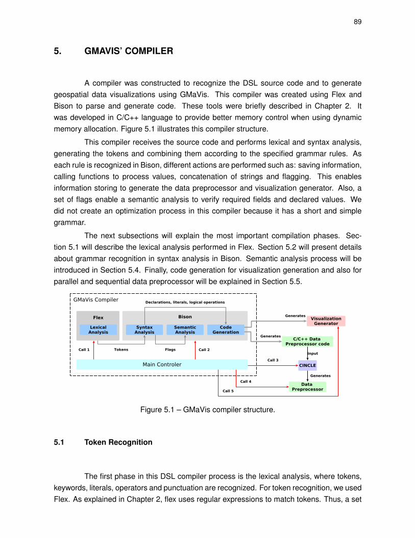
89

5. GMAVIS’ COMPILER

A compiler was constructed to recognize the DSL source code and to generategeospatial data visualizations using GMaVis. This compiler was created using Flex andBison to parse and generate code. These tools were briefly described in Chapter 2. Itwas developed in C/C++ language to provide better memory control when using dynamicmemory allocation. Figure 5.1 illustrates this compiler structure.

This compiler receives the source code and performs lexical and syntax analysis,generating the tokens and combining them according to the specified grammar rules. Aseach rule is recognized in Bison, different actions are performed such as: saving information,calling functions to process values, concatenation of strings and flagging. This enablesinformation storing to generate the data preprocessor and visualization generator. Also, aset of flags enable a semantic analysis to verify required fields and declared values. Wedid not create an optimization process in this compiler because it has a short and simplegrammar.

The next subsections will explain the most important compilation phases. Sec-tion 5.1 will describe the lexical analysis performed in Flex. Section 5.2 will present detailsabout grammar recognition in syntax analysis in Bison. Semantic analysis process will beintroduced in Section 5.4. Finally, code generation for visualization generation and also forparallel and sequential data preprocessor will be explained in Section 5.5.

Figure 5.1 – GMaVis compiler structure.

5.1 Token Recognition

The first phase in this DSL compiler process is the lexical analysis, where tokens,keywords, literals, operators and punctuation are recognized. For token recognition, we usedFlex. As explained in Chapter 2, flex uses regular expressions to match tokens. Thus, a set

90

of regular expressions was created to recognize each token required in this DSL. Initially, afile with the required format of Flex was created. Then, a set of regular expressions werecreated for each token recognized in the source code. This enabled the creation of an initialscanner that reads the input source code and generates tokens. These tokens are used toverify if the source code follows the grammar and for code generation.

In GMaVis, some keywords were defined to express declarations or specific infor-mation. For example, the keyword f̈ilterïs used in a filter declaration, which works combinedwith a logical expression. When the lexer reads the word filter, it generates a token for thissince there is a regular expression in our scanner that recognizes this. The same operationis performed for other keywords, punctuation and literals. The following regular expressionswere used to recognize the entire DSL.

The regular expressions were inserted in a flex file with a .l extension. This file issplit into three parts: definitions, rules, and user code. Initially, we inserted some variablesused to control the line number and token location in the file. This enabled the creationof message errors with the exact token location in the input source code. Also, this firstpart allows the insertion of the bison file declaration and C/C++ libraries to be used in thecompiler. In the second section of GMaVis flex file, we inserted an important option %option

caseinsensitive to disable the case-sensitive recognition in this compiler. Since the mainobjective was to facilitate the use of this DSL, the GMaVis compiler does not differentiateupper-case from lower-case letters. Thus, if the user creates a code with the work F̈ilterörf̈ilter,̈ the scanner will recognize it as the same token. Also, in this section, it was insertedthe regular expressions to recognize the tokens. When the scanner recognizes a particularregular expression in the input source code, it can generate an action. In this specific case,the scanner creates a token and returns it to Bison to use in grammar recognition. GMaVisdo not need to recognize spaces and escape characters. Therefore, when the scannerrecognizes one of these no action is performed. The third section in a flex file was not usedin this compiler since all the control is performed in the bison file. Next section describes thisfile.

5.2 Grammar Recognition

An important part of this compiler is the Bison file with the .y extension. This con-tains all the grammar expressed in a YACC format as well as, some functions such as main,the tokens declarations, token type declarations, and the actions for each grammar rule. Thegeneral concept is that when Flex recognizes the tokens, bison stores them in a stack andperforms a shift or a reduce operation using the grammar rules, as explained in Chapter 2.Then a reduce in some grammar rules is performed, which results in an action. For exam-

91

ple, this action can be to generate code, store important information, recover from an erroror report some information to users.

In GMaVis compiler, different actions are performed for each grammar rule. Also,GMaVis grammar is very simple, so an AST (Abstract Syntax Tree) was not required. Be-cause it is a description language, we instead used flags to verify semantic errors, as ex-plained in Section 5.4. Therefore, the actions performed in each grammar rule were reduced.Also, creating an AST would require more execution time and memory, therefore not doingso enabled a faster and low memory consumption compiler. Thus, only four different actionsare performed when a rule is matched: to set flags, store source code information, generatelogical expression code, and report important information during parsing. Each action isexplained in the next section.

5.2.1 Flag Setting

Flags were used to enable a code verification about which fields were declared,type of information used, literals and data formats specified in input source code. Theseflags are logical variables, which receive a true or false value. A flag is set initially as falseand when it receives a true value when set. In this compiler the following variables wereused as flags.

date_format_required: It is true when a field that receives a value uses a literal date.Through this flag, it is possible to verify required functions and special dealing withdate formats in code generation. Also, we can check in the semantic analysis if aformat for data was given. If not, a semantic error is reported.

delimiter_special and end_register_special: These flags, when true, inform that the userspecified a special character as a delimiter and did not use the tab or newline reservedword of GMaVis. In this case, the compiler may perform an operation of removingquotes from the string returned by the scanner analysis to print this delimiter in thegeneration of code.

do_marker_text and first_marker_field: These flag are set when the field marker-text isrecognized in the input source code. This flag is used in code generation for both datapreprocessor and visualization generator since a markedmap visualization without atext for each marker is differently generated of when using this feature.

do_classification: This flag is set when the compiler recognizes the declaration of a clas-sification block. It is required since a visualization that uses classification is generatedwith different icons and information and visualizations without classification are sim-

92

pler. Also, in data pre-processing, different actions are performed when a classificationis required.

date_format_set: This flag informs a declaration of a data-format in input source code. Itis used in the semantic analysis to verify if the data format is declared when a declara-tion receives a literal date as input. For example, if a user declared a filter that uses afield with a date, but no format for this date is declared, the compiler must generate asemantic error.

delimiter_set and end_register_set: These flags are set to inform if users declared thedelimiter or end-register for the input file. These are used in the semantic analysisto generate a semantic error for the user.

location_set: This flag was created for the field location declaration. It may be used in thefuture for new visualizations. Currently, this field is only reserved for future use.

value_set: This flag was created for the field value declaration. It may be used in the futurefor new visualizations. Currently, this field is only reserved for future use.

zoom_set: This flag informs that a zoom declaration was specified. It is used in code gen-eration during the visualization generation phase. If this tag is false, a default zoomvalue is applied.

page_title_set: This flag informs if the declaration page-title was created in the inputsource code. It is used in the visualization generation to choose between inserting astring value from an information variable or generating a default title.

latitude_set and longitude_set: For verifying if the required field latitude was declared,we use this flag in semantic analysis. If it is not set, the compiler reports a semanticerror message.

size_set: The field size informs the size to generate the visualization. If this flag is false,the compiler generates the visualization using a full-size visualization as default. It isonly used in code generation.

Furthermore, the presented flags are used to improve and facilitate code recog-nition, semantic analysis, and code generation. Most flags are used in many phases, andthey are set during the parsing. These flags have enabled a simpler compiler constructionwithout the creation of an AST and functions to browse this. Of course, it is possible sinceGMaVis have a short grammar with a description language and is not implemented insideanother general purpose language.

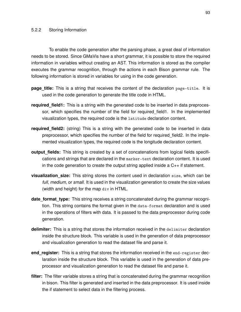
93

5.2.2 Storing Information

To enable the code generation after the parsing phase, a great deal of informationneeds to be stored. Since GMaVis have a short grammar, it is possible to store the requiredinformation in variables without creating an AST. This information is stored as the compilerexecutes the grammar recognition, through the actions in each Bison grammar rule. Thefollowing information is stored in variables for using in the code generation.

page_title: This is a string that receives the content of the declaration page-title. It isused in the code generation to generate the title code in HTML.

required_field1: This is a string with the generated code to be inserted in data preproces-sor, which specifies the number of the field for required_field1. In the implementedvisualization types, the required code is the latitude declaration content.

required_field2: (string) This is a string with the generated code to be inserted in datapreprocessor, which specifies the number of the field for required_field2. In the imple-mented visualization types, the required code is the longitude declaration content.

output_fields: This string is created by a set of concatenations from logical fields specifi-cations and strings that are declared in the marker-text declaration content. It is usedin the code generation to create the output string applied inside a C++ if statement.

visualization_size: This string stores the content used in declaration size, which can befull, medium, or small. It is used in the visualization generation to create the size values(width and height) for the map div in HTML.

date_format_type: This string receives a string concatenated during the grammar recogni-tion. This string contains the format given in the data-format declaration and is usedin the operations of filters with data. It is passed to the data preprocessor during codegeneration.

delimiter: This is a string that stores the information received in the delimiter declarationinside the structure block. This variable is used in the generation of data preprocessorand visualization generation to read the dataset file and parse it.

end_register: This is a string that stores the information received in the end-register dec-laration inside the structure block. This variable is used in the generation of data pre-processor and visualization generation to read the dataset file and parse it.

filter: The filter variable stores a string that is concatenated during the grammar recognitionin bison. This filter is generated and inserted in the data preprocessor. It is used insidethe if statement to select data in the filtering process.

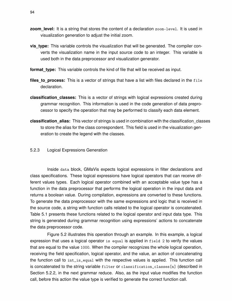
94

zoom_level: It is a string that stores the content of a declaration zoom-level. It is used invisualization generation to adjust the initial zoom.

vis_type: This variable controls the visualization that will be generated. The compiler con-verts the visualization name in the input source code to an integer. This variable isused both in the data preprocessor and visualization generator.

format_type: This variable controls the kind of file that will be received as input.

files_to_process: This is a vector of strings that have a list with files declared in the file

declaration.

classification_classes: This is a vector of strings with logical expressions created duringgrammar recognition. This information is used in the code generation of data prepro-cessor to specify the operation that may be performed to classify each data element.

classification_alias: This vector of strings is used in combination with the classification_classesto store the alias for the class correspondent. This field is used in the visualization gen-eration to create the legend with the classes.

5.2.3 Logical Expressions Generation

Inside data block, GMaVis expects logical expressions in filter declarations andclass specifications. These logical expressions have logical operators that can receive dif-ferent values types. Each logical operator combined with an acceptable value type has afunction in the data preprocessor that performs the logical operation in the input data andreturns a boolean value. During compilation, expressions are converted to these functions.To generate the data preprocessor with the same expressions and logic that is received inthe source code, a string with function calls related to the logical operator is concatenated.Table 5.1 presents these functions related to the logical operator and input data type. Thisstring is generated during grammar recognition using expressions’ actions to concatenatethe data preprocessor code.

Figure 5.2 illustrates this operation through an example. In this example, a logicalexpression that uses a logical operator is equal is applied in field 2 to verify the valuesthat are equal to the value 1000. When the compiler recognizes the whole logical operation,receiving the field specification, logical operator, and the value, an action of concatenatingthe function call to int_is_equal with the respective values is applied. This function callis concatenated to the string variable filter or classification_classes[n] (described inSection 5.2.2, in the next grammar reduce. Also, as the input value modifies the functioncall, before this action the value type is verified to generate the correct function call.

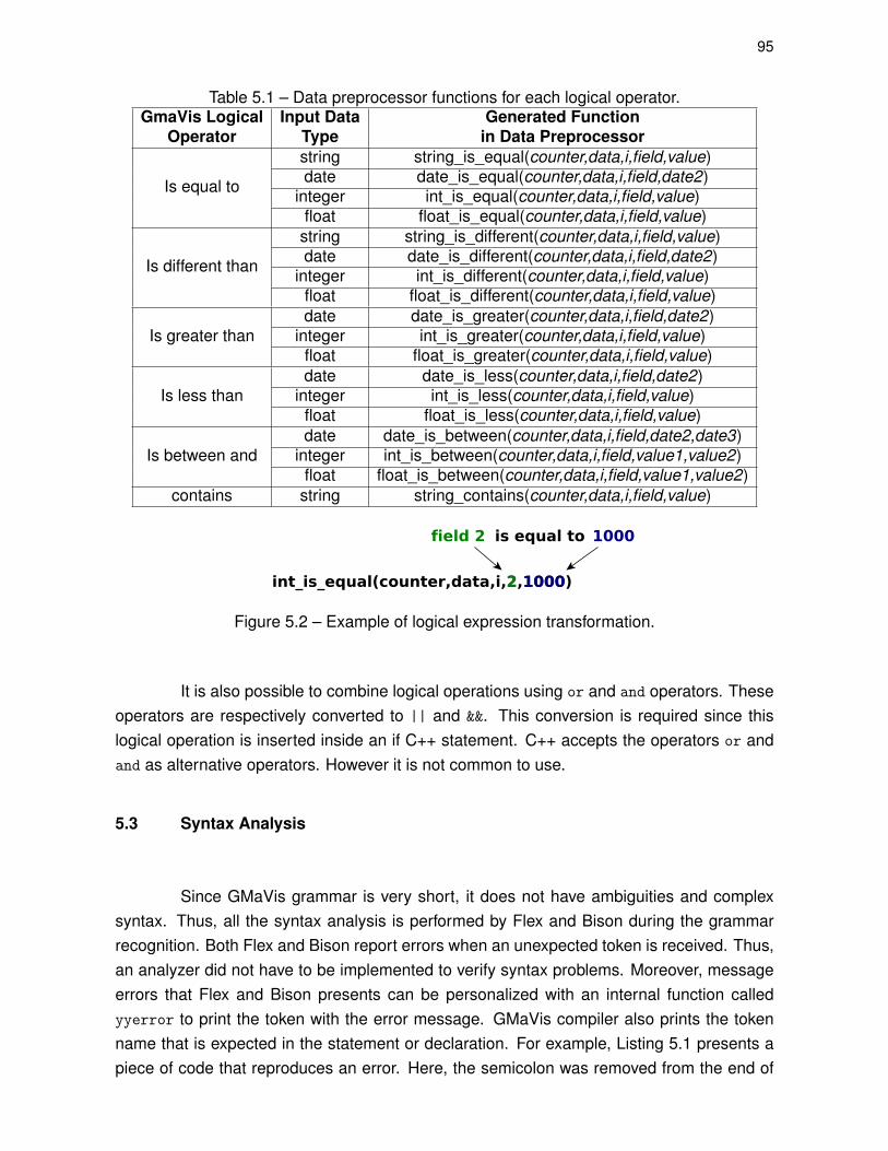
95

Table 5.1 – Data preprocessor functions for each logical operator.GmaVis Logical

OperatorInput Data

TypeGenerated Function

in Data Preprocessor

Is equal to

string string_is_equal(counter,data,i,field,value)date date_is_equal(counter,data,i,field,date2)

integer int_is_equal(counter,data,i,field,value)float float_is_equal(counter,data,i,field,value)

Is different than

string string_is_different(counter,data,i,field,value)date date_is_different(counter,data,i,field,date2)

integer int_is_different(counter,data,i,field,value)float float_is_different(counter,data,i,field,value)

Is greater thandate date_is_greater(counter,data,i,field,date2)

integer int_is_greater(counter,data,i,field,value)float float_is_greater(counter,data,i,field,value)

Is less thandate date_is_less(counter,data,i,field,date2)

integer int_is_less(counter,data,i,field,value)float float_is_less(counter,data,i,field,value)

Is between anddate date_is_between(counter,data,i,field,date2,date3)

integer int_is_between(counter,data,i,field,value1,value2)float float_is_between(counter,data,i,field,value1,value2)

contains string string_contains(counter,data,i,field,value)

Figure 5.2 – Example of logical expression transformation.

It is also possible to combine logical operations using or and and operators. Theseoperators are respectively converted to || and &&. This conversion is required since thislogical operation is inserted inside an if C++ statement. C++ accepts the operators or andand as alternative operators. However it is not common to use.

5.3 Syntax Analysis

Since GMaVis grammar is very short, it does not have ambiguities and complexsyntax. Thus, all the syntax analysis is performed by Flex and Bison during the grammarrecognition. Both Flex and Bison report errors when an unexpected token is received. Thus,an analyzer did not have to be implemented to verify syntax problems. Moreover, messageerrors that Flex and Bison presents can be personalized with an internal function calledyyerror to print the token with the error message. GMaVis compiler also prints the tokenname that is expected in the statement or declaration. For example, Listing 5.1 presents apiece of code that reproduces an error. Here, the semicolon was removed from the end of

96

a latitude declaration in line 4. Thus, it may reproduce an error in line 5 when it finds thekeyword longitude.

1 v i s u a l i z a t i o n : markedmap ;2

3 s e t t i n g s {4 l a t i t u d e : f i e l d 125 long i t ude : f i e l d 11;6 . . .7 }8 . . .

Listing 5.1 – Syntax error example.

When compiling a code with this syntax error, it will reproduce the error messageillustrated in Figure 5.3. This error message informs the error line in the source code, theinformation of a syntax error, the unexpected token received and which token should bereceived to match with the grammar rule in Bison.

Figure 5.3 – Error example for a syntax error.

Bison default configurations do not report an error informing the unexpected andexpected token in the syntax error message. A configuration in the Bison file (.y) had to beset to accept report errors with more details. Thus, it was declared %define parse.error

verbose. It forces Bison to present errors with detailed information.

5.4 Semantic Analysis

Semantic analysis is performed through the flags, as explained in Section 5.2.Since this is a description language with a simple grammar, the construction of an AST bothto generate code or implement the code analysis was not required. It is possible to verify ifthe inserted code is correct and have the required information to generate the visualizationthrough flags that receive boolean values during grammar recognition.

The semantic verification is simple. It verifies if required declarations for specificcases are correct. For example, the following algorithm describes one of the verificationsperformed. In this example, it is verified if the fields for longitude and latitude were de-clared when the visualization is a markedmap. If this analysis finds a false value, the algorithmreturns an error to the user.

The previous example shows only two verifications performed in the semantic anal-ysis. However, there are more 15 verifications that when false returns the following errorsmessages.

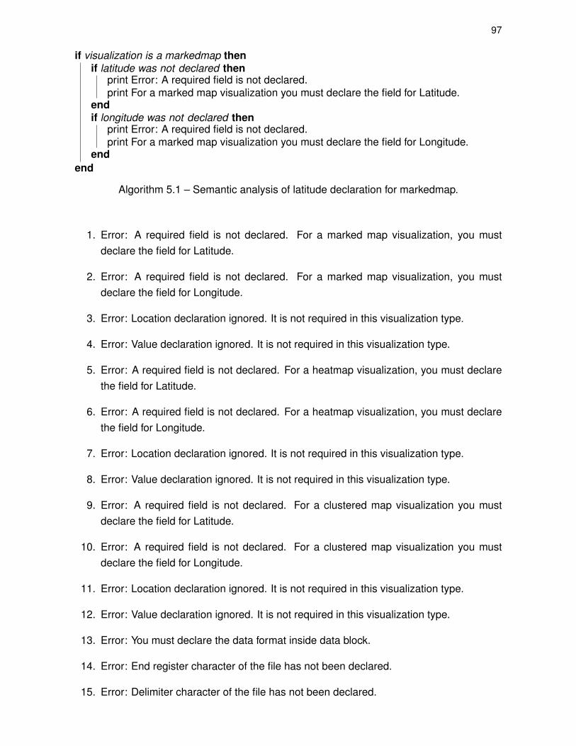
97

if visualization is a markedmap thenif latitude was not declared then

print Error: A required field is not declared.print For a marked map visualization you must declare the field for Latitude.

endif longitude was not declared then

print Error: A required field is not declared.print For a marked map visualization you must declare the field for Longitude.

endend

Algorithm 5.1 – Semantic analysis of latitude declaration for markedmap.

1. Error: A required field is not declared. For a marked map visualization, you mustdeclare the field for Latitude.

2. Error: A required field is not declared. For a marked map visualization, you mustdeclare the field for Longitude.

3. Error: Location declaration ignored. It is not required in this visualization type.

4. Error: Value declaration ignored. It is not required in this visualization type.

5. Error: A required field is not declared. For a heatmap visualization, you must declarethe field for Latitude.

6. Error: A required field is not declared. For a heatmap visualization, you must declarethe field for Longitude.

7. Error: Location declaration ignored. It is not required in this visualization type.

8. Error: Value declaration ignored. It is not required in this visualization type.

9. Error: A required field is not declared. For a clustered map visualization you mustdeclare the field for Latitude.

10. Error: A required field is not declared. For a clustered map visualization you mustdeclare the field for Longitude.

11. Error: Location declaration ignored. It is not required in this visualization type.

12. Error: Value declaration ignored. It is not required in this visualization type.

13. Error: You must declare the data format inside data block.

14. Error: End register character of the file has not been declared.

15. Error: Delimiter character of the file has not been declared.

98

5.5 Code Generation

Code generation is performed in two steps in this compiler. First the data prepro-cessor is generated to process input data. This first generation uses the information receivedin block data to open input files and apply filter and classification. Also, information aboutfile structure is used to parse the file. The second code generation creates the visualiza-tion. It receives the output file with the formatted data from data preprocessor and createsthe visualization file in HTML inserting both code and data. Also, a parallel version of datapreprocessor was implemented using SPar. We inserted annotations in the sequential codeto compile this parallel version using the SPar compiler, called Cincle.

Information stored in variables and flags, as described in Section 5.2.2 enables thiscode generation. Since the information required to generate are stored in variables, it is easyto insert them in the correct place in the generation. Thus, this code generation becomesvery simple. The major difficulty is to handle uncommon pieces of code when generatingdifferent visualization types. This is difficult because input data may or may not be classified,have markers, have a legend for classes and filtering that can modify the final visualizationcode.

The next subsections will explain how code generation is performed in this com-piler. Subsection 5.5.1 will describe the code generation for the data preprocessor. Subsec-tion 5.5.2 details the generation realized for the parallel version of data preprocessor usingSPar. Finally, Section 5.5.3 explains the code generation for visualization generation.

5.5.1 Data Preprocessor Generator

The data preprocessor is generated to perform operations such as filtering, clas-sifying, data selection and formatting. These operations are realized through functions thatparse, process and save the output data. The generation of a data preprocessor consistsof printing in a file with the name data_preprocessor.cpp the code and call the G++ com-piler. After the parallel version is implemented, it is not required to call G++, even if the codegenerated is sequential since the SPar compiler also enables the generation of sequentialcode. This is explained in detail in Subsection 5.5.2. Thus, we basically follow the workflowillustrated in Figure 5.4 where the data preprocessor generator receives the variables withinformation about files to be processed, data structure, date formats, filter, and classes fromthe code analyzer. This information is generated with the code for data preprocessor.

The use of flags in this phase is very important. This generation also requiresinformation about the flags about declarations to know how the data preprocessor will beimplemented. For example, if the data visualization does not require classification, it is not

99

Figure 5.4 – Data preprocessor generation.

necessary to include functions and variables that are used to perform a classification in datapreprocessor. The same applies for filtering and text in markers. Furthermore, flags are usedin the creation of functions to generate output since it needs to know how much informationand what fields must be printed.

This code generation requires special attention to the following steps since depend-ing on the input GMaVis code the data preprocessor is modified.

Input Files Input files are inserted in the main data pre-processing code, which sends afunction called process(). The list of files received during the grammar recognition isused in this phase of code generation. The path to the file is written in the main codeenabling the data preprocessor to read and process each one.

Data Structure Data structure information is used to parse the input file. The delimiter andthe end register character are informed in the DSL code. This information is now storedin a string. This string is copied to the data_preprocessor variables inside process()

function.

Date Format Dealing with date requires some additional processing that is not in othervalue types. In GMaVis the users specify a date using a string and must insert theformat of this date also, since data preprocessor cannot recognize this automatically.Users specify the format of this data through the date format declaration. In codegeneration this information is used to generate the logical operators that deal withthe date: date_is_equal(...), date_is_different(...), date_is_greater(...), date_is_less(...)and date_is_between(...).Also, to inform data value, the user may specify the keyworddate before the string.

Filters Filters generation is performed using the information stored in the variable filters,which receives a logical expression as explained in Section 5.2.3. These filters aregenerated inside an if in the filter function.

100

Classification Classification generation inside data preprocessor is similar to the filters.The main difference here is that we can have many classes. Each class is writteninside the function classification in the data preprocessor.

Output Saving Function This phase in data pre-processing requires special attention forvisualizations that have markers with text and classification. The addition of these twopieces of information in the output file results in more columns, and consequently, a dif-ferent code generated. Markers’ text information are stored in a variable as explainedin Section 5.2.2. It requires additional processing for concatenating strings and fieldcontents specified in the declaration marker-text. Classification fields are simple tohandle in the output since they do not require any concatenation, just a print of a newcolumn at the end of the file.

5.5.2 Data Preprocessor in Parallel

Preliminary results [LGMF15] through execution time using three data loads con-cluded that the data preprocessor module has a high computational cost when working withbig files. To speed up the data pre-processing and enable efficient use of multi-core archi-tectures that have multiple cores, we implemented a parallel version that takes advantage ofparallel architectures with shared memory. Furthermore, the GMaVis compiler was requiredto generate this data preprocessor in parallel, abstracting complexities of visualization cre-ation and parallelism from users. Users of GMaVis do not have contact with parallel codesince it is totally abstracted.

To implement a parallel data preprocessor, we need to understand how a singleprocess runs when in a sequential version. Basically Figure 5.5 illustrates a dataset that ispartitioned in N pieces. These pieces are processed sequentially through the three stagesof data processing. The first represents the loading of the file to memory and verification fordata consistency, represented by STR in the figure. The second stage is the data parsing,application of filters, and classification. In this figure, this stage is illustrated using PRO.Finally, a stage receives a string with the output and writes this down in a file. This stage isrepresented by OUT. Thus, each piece of data flows through each stage until the output datais achieved. In the sequential version, a single process performs each operation for eachtime unit, resulting in a higher execution time as the input increases.

As verified, the data preprocessor has an explicit pipeline. It is complex to par-allelize with some interfaces based on loop/iteration decomposition or parallel tasks, suchas OpenMP. However, it is possible to parallelize this problem using interfaces that supportproblem decomposition using a stream parallelism model, as described in Chapter 2. Fig-ure 5.6 illustrates how it is possible to parallelize a data preprocessor using a pipeline modelthat overlaps time through performing the three stages in different processors. Thus, we

101

Figure 5.5 – Example of sequential processing in data preprocessor.

considered using three parallel programming interfaces to parallelize the data preprocessorand, generate it using this interface. TBB, Fastflow, and SPar enabled the parallelization ofthis software.

Figure 5.6 – Parallel preprocessor using pipeline strategy.

Looking to speed up the pre-processing generation, we used SPar to generate aparallel version of data preprocessor. As previously mentioned, we considered implementingthis using TBB and Fastflow. SPar was chosen because it facilitates code generation in theGMaVis compiler. SPar uses annotations to generate parallel code. Thus, the code thatwe implemented to parallelize the data preprocessor using SPar is almost the same as is

102

used in the sequential version. To parallelize this software, just a few lines of code had to beimplemented in the sequential version. Figure 5.7 illustrates the function process, which hasthe three stages. Here we inserted the three lines of code that SPar requires to parallelizethe code for the strategy illustrated in Figure 5.6. Figure 5.8 illustrates the same sequential.

Figure 5.7 – Illustration of process function code with SPar annotations.

Figure 5.8 – Illustration of sequential process function code.

It is possible to verify that SPar requires few modifications in the sequential codeto parallelize. If we use TBB or FastFlow to parallelize this function, it would require imple-menting additional code to create this same parallel version. Therefore, using SPar, we hada faster and easier parallel code generator implementation. Moreover, SPar’s compiler alsoenables us to compile both sequential and parallel code with the same annotated code, just

103

changing a command line parameter. Hence, the same code illustrated in Figure 5.7 en-ables the creation of both executables since it keeps the same semantic implementation. Ifwe need a sequential executable, the parameter -cincle must be removed from the compilercommand line. This makes the G++ compiler ignore the annotations of SPar and generatesa sequential executable.

5.5.3 Data Visualization Generator

The data visualization generator uses some information to create the visualization.First it receives information from the parser, using flags and stored strings to create an HTMLfile with both code and data. It also receives the file containing the output data previouslyprocessed in data preprocessor as input. It opens the file with the output data, and insertseach element, code or information in a specific location. Information received from thecompiler is described as follows.

Auto Focus One piece of information required in Google Maps API is the latitude and longi-tude to focus the first visualization load. Usually, the user informs this, however, whendealing with many points it is hard to verify this manually. Thus, the data visualizationgenerator calculates this based on the average latitude and longitude of generatedmarkers, using the following equation. Consider n as the total number of registers tobe shown in the visualization. It calculates the average latitude and longitude registersto create the centering position values.

latitude-focus =

n�i=1

latitudei

n(5.1)

longitude-focus =

n�i=1

longitudei

n(5.2)

Visualization Type Depending on the visualization, a different code is generated. Thisinformation is received and is the first verification before starting the generation.

Data Structure It is used to read the file. The data preprocessor generates the output withthe same delimiters of the original data. Then, this phase of generation requires thisinformation to read the output.

Classification It is required to know if there is a classification applied in the output data.This will require implementing different icons for markers and, if declared in the sourcecode, a legend.

104

Title This is used to create a page with the same title informed in the source code.

Size It is used to create the visualization with the size declared. It can be small, medium orfull.

Marker Text Information about marker text is required to create values to show when mark-ers are clicked.

Figure 5.9 illustrates the generation process in the data visualization generator. Animportant aspect is that there are pieces of code that are common in any visualization. Thesepieces of code are always generated directly, without any verification in the declarations ordata. However, there are specific pieces of code that are related to the received sourcecode, and these specific pieces of codes have to specially verify the visualization type, data,classifications and other details. In the data visualizations implemented, there is a specificplace where data is inserted. Also, different visualizations implement different formats forinserting this data like arrays or variables for each marker. Because there is not a commonway to insert this, the data visualization generator formats the data for each visualization.

Figure 5.9 – Data visualization generation.

The generated visualization uses Google Maps API to display the map and visualelements. This API was chosen because it offers a set of visualizations with an easy im-plementation, facilitating code generation. Also, Leaflet and OpenLayers, were analyzed,but they have complex libraries and do not offer significant gains for GMaVis. Even usingGoogle Maps API, it is possible to implement visualizations from others libraries since it iscreated in a similar way. To do so, one must understand the library and how the informationcan be inserted.

105

6. EVALUATION AND DISCUSSION

This chapter presents the methodology used and results obtained with the GMaVisevaluation. Section 6.1 presents the methodology used to evaluate this DSL. As previouslyexplained, we divided this evaluation into two parts. First, we analyzed the programmingeffort and code productivity with GMaVis and other map implementation tools. Second, weconducted a performance analysis to evaluate GMaVis’ compiler and its code generation.Thus, Section 6.2 presents the results for the first experiments. Section 6.3 explains theperformance analysis results.

6.1 Methodology

In order to validade GMaVis productivity and performance of parallel processing,some research questions and hipotheses were defined. Subsection 1.3.1 describes theseresearch questions and some hypotheses. To validate GMaVis and answer the researchquestions, two different evaluations were performed. The first evaluation, described in Sub-section 6.1.2, is an analysis of the programming effort to validate the effectiveness of fa-cilitating visualization creation with GMaVis. This evaluation compares the effort to createa visualization using GMaVis and traditional tools, through COCOMO [Boe81] and SLOC-Count [Whe16] estimation results. The second evaluation, explained in Subsection 6.1.3, isabout performance. It evaluates the parallel data preprocessor to verify if it achieves betterperformance compared to the sequential version. Since TBB [Rei07] was also consideredto be used to parallelize data preprocessor module because it offers stream parallelism sup-port, we compared its aplication to SPar. This comparison verifies if a parallelized TBBversion presents better results than the automatic generated SPar version of data prepro-cessor.

6.1.1 Applications and Input Datasets

Both evaluations (programming effort and performance) used the applications pre-sented in the Subsection 4.5.2. These applications use different features provided by GMaVis,such as filters, classification, file structure specification, and logical operators. Moreover,these applications were implemented using Google Maps API, Leaflet, and OpenLayers inorder to compare the effort required to create a visualization using GMaVis to different li-braries with the same purpose. Also, the same datasets described in Subsection 4.5.1 wereused in these evaluations, but, for performance evaluation, these datasets were replicated

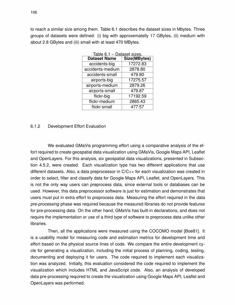
106

to reach a similar size among them. Table 6.1 describes the dataset sizes in Mbytes. Threegroups of datasets were defined: (i) big with approxematelly 17 GBytes, (ii) medium withabout 2.8 GBytes and (iii) small with at least 470 MBytes.

Table 6.1 – Dataset sizes.Dataset Name Size(MBytes)accidents-big 17272.83

accidents-medium 2878.80accidents-small 479.80

airports-big 17275.57airports-medium 2879.26

airports-small 479.87flickr-big 17192.59

flickr-medium 2865.43flickr-small 477.57

6.1.2 Development Effort Evaluation

We evaluated GMaVis programming effort using a comparative analysis of the ef-fort required to create geospatial data visualization using GMaVis, Google Maps API, Leafletand OpenLayers. For this analysis, six geospatial data visualizations, presented in Subsec-tion 4.5.2, were created. Each visualization type has two different applications that usedifferent datasets. Also, a data preprocessor in C/C++ for each visualization was created inorder to select, filter and classify data for Google Maps API, Leaflet, and OpenLayers. Thisis not the only way users can preprocess data, since external tools or databases can beused. However, this data preprocessor software is just for estimation and demonstrates thatusers must put in extra effort to preprocess data. Measuring the effort required in the datapre-processing phase was required because the measured libraries do not provide featuresfor pre-processing data. On the other hand, GMaVis has built-in declarations, and does notrequire the implementation or use of a third type of software to preprocess data unlike otherlibraries.

Then, all the applications were measured using the COCOMO model [Boe81]. Itis a usability model for measuring code and estimation metrics for development time andeffort based on the physical source lines of code. We compare the entire development cy-cle for generating a visualization, including the initial process of planning, coding, testing,documenting and deploying it for users. The code required to implement each visualiza-tion was analyzed. Initially, this evaluation considered the code required to implement thevisualization which includes HTML and JavaScript code. Also, an analysis of developeddata pre-processing required to create the visualization using Google Maps API, Leaflet andOpenLayers was performed.

107

In order to apply COCOMO model, we used SLOCCount3 tool. It is a software mea-surement tool, which counts the physical source lines of code (SLOC), ignoring empty linesand comments. It also estimates development time, cost and effort based on the original Ba-sic COCOMO1 model. The suite supports a wide range of both old and modern programminglanguages (e.g., C++, Javascript, HTML, and CSS), which are naturally inferred by SLOC-Count and thus used for measurement [Whe16]. SLOCCount suite [Whe16] was used bya set of other researches (e.g., [GAF14, LGMF15, AGLF15a, AGLF15b, VSJ+14, SET+09,LRCS14, HFB05, RGBMA06, KEH+09, VSJ+14, STM10]) to measure software complexity.

SLOCCount counts physical lines of code that are also called "non-blank, non-comment lines" in the source code. Furthermore, physical SLOC is defined as a line endingin a newline or end-of-file marker, and that contains, at least, one non-whitespace non-comment character. Comment delimiters (characters other than newlines starting and end-ing a comment) are considered comment characters. Data lines only including whites-pace (e.g., lines with only tabs and spaces in multiline strings) are not included in thecount [Whe16].

After counting physical lines, SLOCcount performs an estimation of effort and sched-ule required to develop the input source code. To express effort, SLOCcount uses person-years and person-months units. Moreover, to express schedule, it uses the total years andmonths as units. When users use SLOCCount in default mode, the "Basic COCOMO" modelis set. This model includes the effort estimation about the whole cycle to develop an appli-cation, such as design, code, test, and documentation time (both user, administrator anddevelopment documentation). This is important to consider when verifying the results sinceit produces high-cost estimates [Whe16].

The basic COCOMO model is usually enough to estimate development effort, butit can produce limited accuracy. When using the basic COCOMO, users do not take someimportant factors into consideration. In order to improve accuracy users can use the "Inter-mediate COCOMO" and "Detailed COCOMO" models that have some factors to perform amore detailed estimation. These enable more accurate results. Thus, if the sloccount userhas information about the domain, developers, development environment and other details,it can be used to improve the model’s accuracy. It is possible to change the –effort and–schedule factor parameters in the SLOCCount command line. Another important questionto determine when using SLOCCount with "detailed COCOMO" is the application’s mode,which can be "Organic", "embedded", or "semidetached". "Organic" is the default configu-ration used in Sloccount because most applications are in this category [Whe16]. Table 6.2shows the difference between the software models available in COCOMO model.

In the COCOMO model, it is possible to use some corrective factors to determineeffort. These factors are called cost drivers and enable a detailed analysis of effort accordingto the application, developers, environment and other issues that affect the development

1http://www.dwheeler.com/sloccount/sloccount.html#cocomo

108

Table 6.2 – Software category in COCOMO model (Adapted from [Whe16]).Category DescriptionOrganic Relatively small software teams develop software in a highly familiar, in-house

environment. It has a stable development environment, minimal need forinnovative algorithms, and requirements can be relaxed to avoid extensiverework.

Semidetached This is an intermediate step between organic and embedded. This is charac-terized by reduced flexibility in the requirements.

Embedded The project must operate within tight (hard-to-meet) constraints, and require-ments and interface specifications are often non-negotiable. The softwarewill be embedded in a complex environment that the software must deal withas-is.

cycle. Each cost driver has a value that is used to calculate the effort through the productof all factors. The result is the final effort factor. Table 6.3 presents the cost drivers. Thechosen values for this analysis have highlighted cells.

Table 6.3 – COCOMO cost drivers (Adapted from [Whe16]).Cost Drivers Ratings

ID Driver Name Very Low Low Nominal High Very High Extra High

RELY Required softwarereliability 0.75 0.88 1.00 1.15 1.40 -

DATA Database size - 0.94 1.00 1.08 1.16 -CPLX Product complexity 0.70 0.85 1 1.15 1.3 1.65TIME Execution time constraint - - 1.00 1.11 1.30 1.66STOR Main storage constraint - - 1.00 1.06 1.21 1.56VIRT Virtual machine volatility - 0.87 1.00 1.15 1.30 -TURN Computer turnaround time - 0.87 1.00 1.07 1.15 -ACAP Analyst capability 1.46 1.19 1.00 0.86 0.71 -AEXP Applications experience 1.29 1.13 1.00 0.91 0.82 -PCAP Programmer capability 1.42 1.17 1.00 0.86 0.70 -VEXP Virtual machine experience 1.21 1.10 1.00 0.90 - -

LEXP Programming languageexperience 1.14 1.07 1.00 0.95 - -

MODP Use of "modern"programming practices 1.24 1.1 1.00 0.91 0.82 -

TOOL Use of software tools 1.24 1.1 1.00 0.91 0.83 -

SCED Required developmentschedule 1.23 1.08 1.00 1.04 1.10 -

Some cost drivers were set for this experiment to achieve more accurate results.These driver costs were used to measure all the libraries and GMaVis. Some cost driverswere not used since they do not make sense and do not apply to this case. For example,virtual machine volatile was not considered in this analysis since we do not use or havevirtual machines in the environment. Thus, in this case, we set this as a nominal value(1.00). Each value considered in this analysis is explained bellow.

Required software reliability This measure represents required software reliability. Forexample, if a software failure would risk human life, then it may be set to very high.

109

Product complexity This represents the complexity of the final product. For this measure,it is important to consider the following areas that can generate complexities in thesoftware: control, computation, device-dependent, or data management operations.

Applications experience It expresses the knowledge and experience of a developer orteam about applications that support development, such as IDEs, programming li-braries, frameworks and other tools.

Programmer capability Similar to the previous item, this measure considers the overallknowledge of a team or developer. This includes not only applications, but also analy-sis, communication, team cooperation, and interaction.

Programming language experience It is related to the level of knowledge and experienceabout the project programming language and software tool. Developers with moreexperience in the programming language can create software with less effort than adeveloper with low-level knowledge.

Use of "modern" programming practices This represents the use of modern program-ming practices. It includes code reuse, top-down incremental development, structureddesign notation, top-down requirements analysis and design, design and code walk-throughs or inspections, structured code, use of libraries and other methods that im-prove and facilitate development.

Use of software tools This measure is related to the use of software that facilitates thedevelopment such as IDEs, programming libraries, frameworks and other tools.

To generate effort based on the attributes, each attribute is rated using one of sixvalues from "very low" to "extremely high". Then, each value implies in an effort multiplierthat results in an effort adjustment factor (EAF) [Boe81]. Thus, EAF can be used to improvethe accuracy of estimation in SLOCCount. Moreover, SLOCCount performs the followingcalculus automatically, it will be presented the intermediate COCOMO model as follows:

(Effort)E = ai (KLOC)bi x EAF (6.1)

(Development time)D = ci(Effort Applied)di (6.2)

(People required)P = Effort/Development Time (6.3)

Where the given ai , bi , ci , and di are based on the values in table 6.4.

110

Table 6.4 – Effort estimation in COCOMO model variables (Extracted from [Whe16]).Software Model ai bi ci di

Organic 2.4 1.05 2.5 0.38Semi-detached 3.0 1.12 2.5 0.35

Embedded 3.6 1.20 2.5 0.32

Based on this table and in the chosen values, the following calculus was used togenerate the effort adjustment factor(EAF).

EAF = 0.75 × 0.70 × 1.13 × 0.70 × 0.95 × 0.82 × 0.83 = 0.2685 (6.4)

In this analysis, we used the organic software model. Thus, in order to calculatethe effort to sloccount, the following calculus multiplying the EAF by the Organic softwaremodel value of 2.4 was performed.

Effort = 2.4 × 0.2685 = 0.6444 (6.5)

Considering that the exponent for effort in an organic model is 1.05, the followingcommand were used to call SLOCCount and measure the effort estimation.

sloccount –effort 0.6444 1.05 <source_project>

Finally, this command line was called inside the project folder of each visualiza-tion. This was also used for data preprocessor analysis. This command results in datawith information about the total physical source lines of code, estimated development effortin person-years and person-months, estimated schedule in years and months, estimatedaverage number of developers, and total estimated cost to develop.

6.1.3 Performance Evaluation

Initially, we performed a preliminary evaluation of the execution time when process-ing huge quantities of data. For these tests, we replicated the YFFCC100M data set toachieve 100GB of data. We did a measurement of 10GB, 50GB, and 100GB to verify thetime it takes for processing. With these results it was possible to conclude that it wouldbe interesting to implement a parallel version of data processing, enabling it to generate avisualization using a huge dataset, for example 1 TBytes, in a reasonable amount of time.

With the parallel version of the data preprocessor, we performed a comparison be-tween the sequential and parallel version with different input sizes to measure the through-put of applied parallelism. Speedup and efficiency calculus were considered in this analysis.However, execution time and throughput were enough to express the results and performs

111

the comparisons required in this context. In this evaluation, each algorithm was executedten times for each input size and number of processors, both in a parallel and sequentialversion. These tests were performed using a multi-core computer Blade Dell PowerEdgeM610 with the following specification.

• Two processors Intel Xeon Six-Core E5645 2.4GHz Hyper-Threading

• 24 GBytes of memory.

• Software:

– Operational System: Ubuntu 14.04 LTS

– C/C++ Compiler: G++ 5.2

– SPar Compiler: CINCLE

In order to verify if the parallel generation to SPar is efficient, a parallel version ofTBB was implemented by a third person. Both TBB and SPar code were compared usingthe same method for sequential and parallel version.

Considering three dataset sizes presented in Subsection 4.5.1, six applicationsand ten executions were performed. Thus, a total of 180 executions for each sequential andparallel version. Parallel versions were executed both using SPar and TBB, using 3 to 24threads2. Thus, there were 180 executions for sequential version, 4320 for SPar and 4320for TBB parallel version, totaling 8820 executions. Execution time were measured usingthe C++ library std::chrono3. This allowed a timestamp to be created before and after aspecific process, calculating the time it took to perform. Thus, the execution time of thewhole pipeline was collected, including file loading, processing, and output saving.

With the execution time and the input size, it was possible to calculate the through-put. Throughput is the average output of a determined production process per unit time [Rus08].It defines a work in process (WIP) and a determined unity of time, also called cycle time (CT).Little’s Law equation enables the calculation of throughput since it is defined as the relationbetween WIP, cycle time and throughput. In order to measure data preprocessor throughputthis equation was adapted [Gus11] to fit this purpose. Little’s Law equation is presented asfollows.

TH =WIPCT

(6.6)

Applying this equation to this work, consider ti as the execution time of a singleexecution i . As mentioned previously, each execution configuration was performed ten times.

2It starts in 3 because there are three stages in the pipeline (loading, processing and saving output). Thus,parallel versions cannot have less than three threads.

3http://www.cplusplus.com/reference/chrono/

112

Thus, the following equation was used to calculate an average of ten executions of a datapreprocessor generated for a d dataset. We also calculated the standart deviation to verifyvalues consistency.

t̄d =

10�

i=1

tid

10(6.7)

With the average execution time in seconds, for a specific d dataset processed indata preprocessor, it is possible to calculate the throughput using the dataset size sd in bitsusing the equation below.

THd =sd

t̄d(6.8)

Finally, the resulting THd provides the throughput value when processing a deter-mined quantity of data for each time unit. In this analysis, we used a measure in Mbytes/sec-onds.

6.2 Code Productivity Results

To verify if GMaVis offers more code productivity and reduces the effort requiredto implement a visualization, we constructed six applications using the three visualizationtypes offered in GMaVis. Each visualization was created using GMaVis, Leaflet, GoogleMaps API, and OpenLayers and is explained in detail in Section 4.5. GMaVis does not re-quire users to implement software or handle data manually to perform data pre-processing.In these results, we measure the necessary code to automatically implement data process-ing, according to each visualization type. Since some applications do not require filtering orclassifying, we split the code and measured each part. It is possible to verify, in all the graph-ics, that the structuring phase takes much more time. It requires more time to develop dueto the higher number of lines to implement. Before analyzing the results, it is important tohighlight that at first, the development time results can seem very high. However, this mea-sure considers the whole cycle to develop software. It estimates the time to plan, code, test,document and deploy the software.

The graph in Figure 6.1 shows the results for Heatmap applications. It is importantto highlight that this type of visualization does not implement classification. This visualizationtype only displays a layer with different colors to express the frequency of elements in thelocation. It is possible to verify that GMaVis obtained better results than Google Maps API,Leaflet, and OpenLayers since it presents a lower estimation time to develop. Also, it is pos-sible to verify that Leaflet requires less code to implement a map visualization than Google

113

Maps API and OpenLayers. The first application does not implement a filter. This reducesthe required code in data processing for Google Maps API, OpenLayers, and Leaflet.

Programming Effort (to Develop, Test, Document and Deploy)

0

5

10

15

20

GmaVis GoogleMaps OpenLayers Leaflet

De

ve

lop

me

nt

Tim

e (

Ho

urs

)

Application

Heatmap - Airports in World (Hm-Airp)

Main

Structuring

Formating

0

5

10

15

20

GmaVis GoogleMaps OpenLayers Leaflet

De

ve

lop

me

nt

Tim

e (

Ho

urs

)

Application

Heatmap - Traffic Accidents in Porto Alegre (Hm-Accid)

Main

Structuring

Filtering

Formating

Figure 6.1 – Code productivity results for heatmap applications.

Two applications for clustered map were measured. Figure 6.2 present the resultsfor their development time estimation. Similar to the first graph, this shows the effort forboth the main and data pre-processing. Here GMaVis obtained a lower time estimation todevelop since it required fewer lines of code and did not require additional implementationsto process data. Moreover, it is possible to verify that Leaflet kept a similar result comparedwith OpenLayers and Google Maps API. This is because this implementation is for clus-teredmaps and the code required to create it is different from the first heatmap application.Application Airports in World presented less development time than Flickr Photos with

"Computer" tag" since it does not use filtering.

Programming Effort (to Develop, Test, Document and Deploy)

0

5

10

15

20

GmaVis GoogleMaps OpenLayers Leaflet

De

ve

lop

me

nt

Tim

e (

Ho

urs

)

Application

Clusteredmap - Airports in World (Ctr-Airp)

Main

Structuring

Formating

0

5

10

15

20

GmaVis GoogleMaps OpenLayers Leaflet

De

ve

lop

me

nt

Tim

e (

Ho

urs

)

Application

Clusteredmap - Flickr Photos with "Computer" Tag (Ctr-Comp)

Main

Structuring

Filtering

Formating

Figure 6.2 – Code productivity results for clustered map applications.

Even with preliminary results that show less development time for markedmap ap-plications, two data visualizations were created to confirm this. Figure 6.3 shows program-ming effort estimation in development time for these visualizations. Different from the previ-ous results, these use both filtering and classification, requiring more time to develop since itincludes the creation of mechanisms or use of external software. If a user uses a C++ code,it would require the time expressed in the graph. Both visualizations present less develop-ment time in main code for GMaVis. In this example, OpenLayers presented the second

114

less development time in main code, since it required less code to implement this kind ofvisualization.

Programming Effort (to Develop, Test, Document and Deploy)

0

5

10

15

20

GmaVis GoogleMaps OpenLayers Leaflet

De

ve

lop

me

nt

Tim

e (

Ho

urs

)

Application

Markedmap - Photos Classified by Device Camera (Mm-Dev)

Main

Structuring

Filtering

Classifying

Formating

0

5

10

15

20

GmaVis GoogleMaps OpenLayers Leaflet

De

ve

lop

me

nt

Tim

e (

Ho

urs

)

Application

Markedmap - Traffic Accidents in Porto Alegre (Mm-Accid)

Main

Structuring

Filtering

Classifying

Formating

Figure 6.3 – Code productivity results for marked map applications.

SLOCcount also estimates the cost required to implement a software. Figure 6.4and Table 6.5 presents the results in dollars for developing each visualization consideringjust the main code. In this graph, the cost required to perform the pre-processing was notinserted or considered. The following abbreviations were used in this graph.

Ctr-Airp Clusteredmap - Airports in World

Ctr-Comp Clusteredmap - Flickr Photos with "Computer" Tag

Hm-Airp Heatmap - Airports in World

Hm-Accid Heatmap - Traffic Accidents in Porto Alegre

Mm-Dev Markedmap - Photos Classified by Device Camera

Mm-Accid Markedmap - Traffic Accidents in Porto Alegre

Table 6.5 – SLOCCount estimation about cost to develop each application.Application GmaVis Google Maps OpenLayers LeafletCtr-Airp $33,00 $77,00 $105,00 $105,00Ctr-Comp $37,00 $77,00 $63,00 $89,00Hm-Airp $33,00 $96,00 $65,00 $53,00Hm-Accid $37,00 $93,00 $77,00 $53,00Mm-Dev $56,00 $77,00 $49,00 $60,00Mm-Accid $46,00 $98,00 $53,00 $60,00

Here, unlike Mm-Dev application, GMaVis requires less development cost. Thisdemonstrates that even not considering the fact that GMaVis avoids the implementationor use of external software to process data, it can improve productivity for developing the

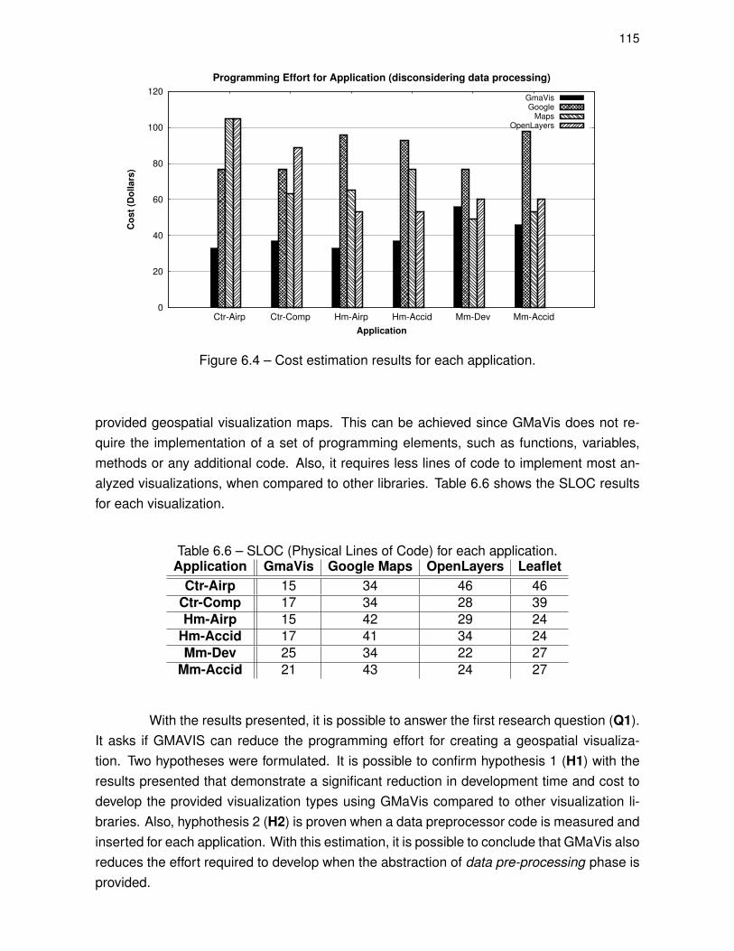
115

0

20

40

60

80

100

120

Ctr-Airp Ctr-Comp Hm-Airp Hm-Accid Mm-Dev Mm-Accid

Co

st

(Do

lla

rs)

Application

Programming Effort for Application (disconsidering data processing)

GmaVisGoogle

MapsOpenLayers

Figure 6.4 – Cost estimation results for each application.

provided geospatial visualization maps. This can be achieved since GMaVis does not re-quire the implementation of a set of programming elements, such as functions, variables,methods or any additional code. Also, it requires less lines of code to implement most an-alyzed visualizations, when compared to other libraries. Table 6.6 shows the SLOC resultsfor each visualization.

Table 6.6 – SLOC (Physical Lines of Code) for each application.Application GmaVis Google Maps OpenLayers Leaflet

Ctr-Airp 15 34 46 46Ctr-Comp 17 34 28 39Hm-Airp 15 42 29 24

Hm-Accid 17 41 34 24Mm-Dev 25 34 22 27

Mm-Accid 21 43 24 27

With the results presented, it is possible to answer the first research question (Q1).It asks if GMAVIS can reduce the programming effort for creating a geospatial visualiza-tion. Two hypotheses were formulated. It is possible to confirm hypothesis 1 (H1) with theresults presented that demonstrate a significant reduction in development time and cost todevelop the provided visualization types using GMaVis compared to other visualization li-braries. Also, hyphothesis 2 (H2) is proven when a data preprocessor code is measured andinserted for each application. With this estimation, it is possible to conclude that GMaVis alsoreduces the effort required to develop when the abstraction of data pre-processing phase isprovided.

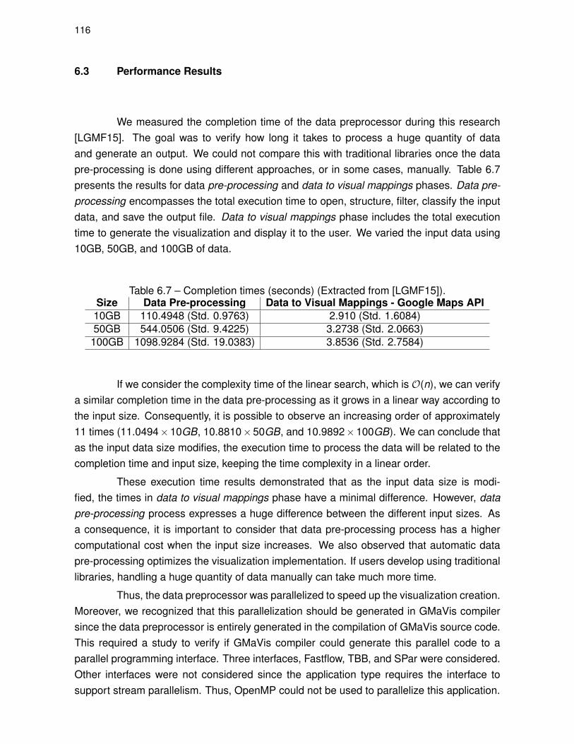
116

6.3 Performance Results

We measured the completion time of the data preprocessor during this research[LGMF15]. The goal was to verify how long it takes to process a huge quantity of dataand generate an output. We could not compare this with traditional libraries once the datapre-processing is done using different approaches, or in some cases, manually. Table 6.7presents the results for data pre-processing and data to visual mappings phases. Data pre-processing encompasses the total execution time to open, structure, filter, classify the inputdata, and save the output file. Data to visual mappings phase includes the total executiontime to generate the visualization and display it to the user. We varied the input data using10GB, 50GB, and 100GB of data.

Table 6.7 – Completion times (seconds) (Extracted from [LGMF15]).Size Data Pre-processing Data to Visual Mappings - Google Maps API10GB 110.4948 (Std. 0.9763) 2.910 (Std. 1.6084)50GB 544.0506 (Std. 9.4225) 3.2738 (Std. 2.0663)100GB 1098.9284 (Std. 19.0383) 3.8536 (Std. 2.7584)

If we consider the complexity time of the linear search, which is O(n), we can verifya similar completion time in the data pre-processing as it grows in a linear way according tothe input size. Consequently, it is possible to observe an increasing order of approximately11 times (11.0494×10GB, 10.8810×50GB, and 10.9892×100GB). We can conclude thatas the input data size modifies, the execution time to process the data will be related to thecompletion time and input size, keeping the time complexity in a linear order.

These execution time results demonstrated that as the input data size is modi-fied, the times in data to visual mappings phase have a minimal difference. However, datapre-processing process expresses a huge difference between the different input sizes. Asa consequence, it is important to consider that data pre-processing process has a highercomputational cost when the input size increases. We also observed that automatic datapre-processing optimizes the visualization implementation. If users develop using traditionallibraries, handling a huge quantity of data manually can take much more time.

Thus, the data preprocessor was parallelized to speed up the visualization creation.Moreover, we recognized that this parallelization should be generated in GMaVis compilersince the data preprocessor is entirely generated in the compilation of GMaVis source code.This required a study to verify if GMaVis compiler could generate this parallel code to aparallel programming interface. Three interfaces, Fastflow, TBB, and SPar were considered.Other interfaces were not considered since the application type requires the interface tosupport stream parallelism. Thus, OpenMP could not be used to parallelize this application.

117

SPar was chosen to parallelize because it facilitates the creation of parallel code.While other interfaces require changes in sequential code to introduce parallelism, SPar onlyrequires the insertion of simple annotations in the sequential code specifying input, output,and replications of stages. To compare the increase of code require to implement the parallelversion of the data preprocessor with SPar and TBB, we used the generated code for thedata preprocessor without SPar annotations, generated code with SPar annotations andTBB implementation of data preprocessors manually created. Table 6.8 demonstrates thesequential and parallel lines of code for the data processor that each application uses.

Table 6.8 – Lines of code to parallelize data preprocessor using SPar and TBB.

Application Sequential SPAR TBBSLOC SLOC Code Increase (%) SLOC Code Increase (%)

CM_CP 210 216 2,857 274 30,476CM_AIR 199 205 3,015 263 32,160HM_AC 210 216 2,857 274 30,476HM_AIR 199 205 3,015 263 32,160MM_DEV 224 230 2,678 288 28,571MM_ACID 216 222 2,777 280 29,629

It is possible to verify that SPar requires fewer lines of code to implement the parallelversion than TBB. This is important in code generation because using SPar hard modifica-tions did not have to be performed in the compiler. A few lines of code had to be addedbefore some statements to inform the beginning of a stream and stage. If we use TBB toparallelize, it would be required to generate functions and change the code. Figure 6.5 high-lights the results in this table, presenting the increase percentage of lines of code comparedwith the sequential version for both SPar and TBB interfaces.

0

5

10

15

20

25

30

35

40

Ctr-Airp Hm-Accid Hm-Airp Mm-Dev Mm-Accid

Inc

rea

se

in

lin

es

of

co

de

(%

)

Applications

SLOC Increase to Parallelize Data Preprocessor

SPar TBB

Figure 6.5 – Comparison of SPar and TBB for parallelize data preprocessor.

Since SPar is in a beta version, under development, it was expected that perfor-mance results would not achieve the same provided by the TBB manually created data

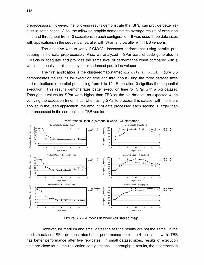
118

preprocessors. However, the following results demonstrate that SPar can provide better re-sults in some cases. Also, the following graphic demonstrates average results of executiontime and throughput from 10 executions in each configuration. It was used three data sizeswith applications in the sequential, parallel with SPar, and parallel with TBB versions.

The objective was to verify if GMaVis increases performance using parallel pro-cessing in the data preprocessor. Also, we analyzed if SPar parallel code generated inGMaVis is adequate and provides the same level of performance when compared with aversion manually parallelized by an experienced parallel developer.

The first application is the clusteredmap named Airports in world. Figure 6.6demonstrates the results for execution time and throughput using the three dataset sizesand replications in parallel processing from 1 to 12. Replication 0 signifies the sequentialexecution. This results demonstrates better execution time for SPar with a big dataset.Throughput values for SPar were higher than TBB for the big dataset, as expected whenverifying the execution time. Thus, when using SPar to process this dataset with the filtersapplied in the used application, the amount of data processed each second is larger thanthat processed in the sequential or TBB version.

Performance Results (Airports in world - Clusteredmap)

0 50

100 150 200 250 300 350 400 450

0 2 4 6 8 10 12Exe

cu

tio

n T

ime

(S

eco

nd

s)

Replicate #

Big Dataset (Execution Time)

TBBSPAR

0

20

40

60

80

100

120

0 2 4 6 8 10 12

Th

rou

gh

pu

t (M

byte

s/s

)

Replicate #

Big Dataset (Throughput)

TBBSPAR

0

10

20

30

40

50

60

70

0 2 4 6 8 10 12Exe

cu

tio

n T

ime

(S

eco

nd

s)

Replicate #

Medium Dataset (Execution Time)

TBBSPAR

0 20 40 60 80

100 120 140 160

0 2 4 6 8 10 12

Th

rou

gh

pu

t (M

byte

s/s

)

Replicate #

Medium Dataset (Throughput)

TBBSPAR

0

2

4

6

8

10

12

0 2 4 6 8 10 12Exe

cu

tio

n T

ime

(S

eco

nd

s)

Replicate #

Small Dataset (Execution Time)

TBBSPAR

0

20

40

60

80

100

120

140

0 2 4 6 8 10 12

Th

rou

gh

pu

t (M

byte

s/s

)

Replicate #

Small Dataset (Throughput)

TBBSPAR

Figure 6.6 – Airports in world (clustered map).

However, for medium and small dataset sizes the results are not the same. In themedium dataset, SPar demonstrates better performance from 1 to 4 replicates, while TBBhas better performance after five replicates. In small dataset sizes, results of executiontime are close for all the replication configurations. In throughput results, the differences in

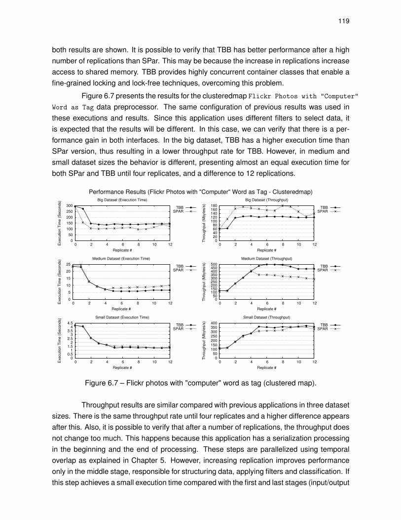
119

both results are shown. It is possible to verify that TBB has better performance after a highnumber of replications than SPar. This may be because the increase in replications increaseaccess to shared memory. TBB provides highly concurrent container classes that enable afine-grained locking and lock-free techniques, overcoming this problem.

Figure 6.7 presents the results for the clusteredmap Flickr Photos with "Computer"

Word as Tag data preprocessor. The same configuration of previous results was used inthese executions and results. Since this application uses different filters to select data, itis expected that the results will be different. In this case, we can verify that there is a per-formance gain in both interfaces. In the big dataset, TBB has a higher execution time thanSPar version, thus resulting in a lower throughput rate for TBB. However, in medium andsmall dataset sizes the behavior is different, presenting almost an equal execution time forboth SPar and TBB until four replicates, and a difference to 12 replications.

Performance Results (Flickr Photos with "Computer" Word as Tag - Clusteredmap)

0

50

100

150

200

250

300

0 2 4 6 8 10 12Exe

cu

tio

n T

ime

(S

eco

nd

s)

Replicate #

Big Dataset (Execution Time)

TBBSPAR

0 20 40 60 80

100 120 140 160 180

0 2 4 6 8 10 12

Th

rou

gh

pu

t (M

byte

s/s

)

Replicate #

Big Dataset (Throughput)

TBBSPAR

0

5

10

15

20

25

0 2 4 6 8 10 12Exe

cu

tio

n T

ime

(S

eco

nd

s)

Replicate #

Medium Dataset (Execution Time)

TBBSPAR

0 50

100 150 200 250 300 350 400 450 500

0 2 4 6 8 10 12

Th

rou

gh

pu

t (M

byte

s/s

)

Replicate #

Medium Dataset (Throughput)

TBBSPAR

0 0.5

1 1.5

2 2.5

3 3.5

4 4.5

0 2 4 6 8 10 12Exe

cu

tio

n T

ime

(S

eco

nd

s)

Replicate #

Small Dataset (Execution Time)

TBBSPAR

0 50

100 150 200 250 300 350 400

0 2 4 6 8 10 12

Th

rou

gh

pu

t (M

byte

s/s

)

Replicate #

Small Dataset (Throughput)

TBBSPAR

Figure 6.7 – Flickr photos with "computer" word as tag (clustered map).

Throughput results are similar compared with previous applications in three datasetsizes. There is the same throughput rate until four replicates and a higher difference appearsafter this. Also, it is possible to verify that after a number of replications, the throughput doesnot change too much. This happens because this application has a serialization processingin the beginning and the end of processing. These steps are parallelized using temporaloverlap as explained in Chapter 5. However, increasing replication improves performanceonly in the middle stage, responsible for structuring data, applying filters and classification. Ifthis step achieves a small execution time compared with the first and last stages (input/output

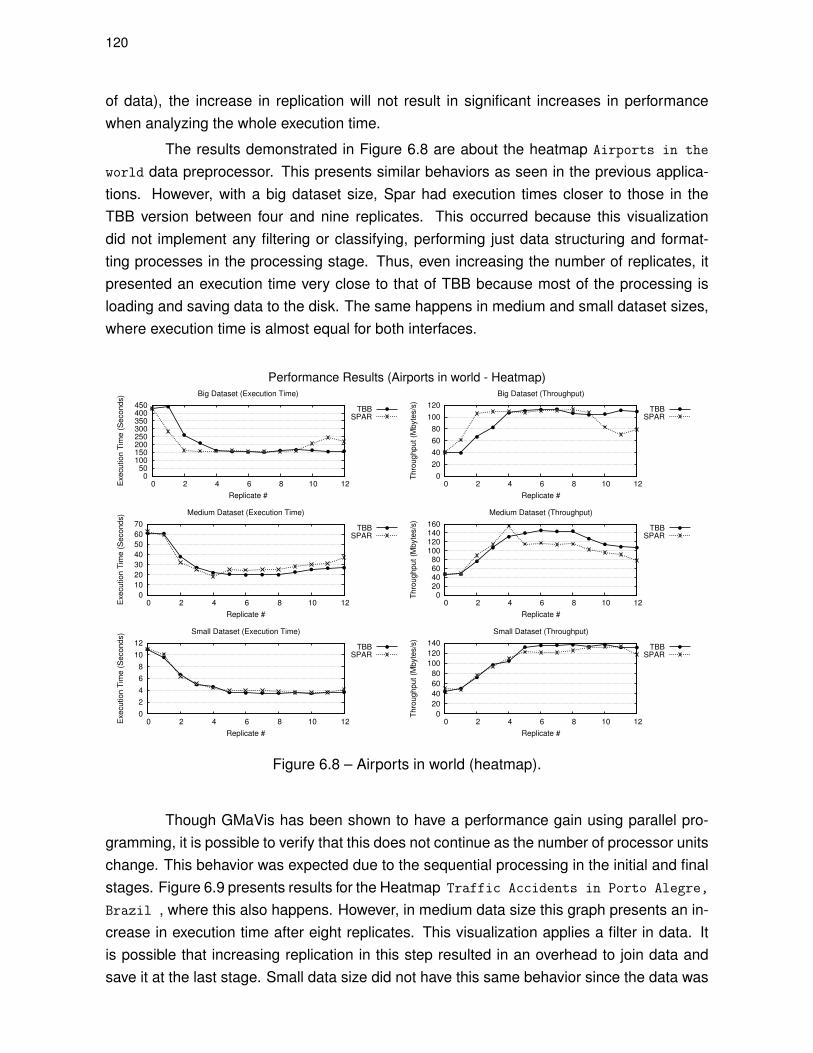
120

of data), the increase in replication will not result in significant increases in performancewhen analyzing the whole execution time.

The results demonstrated in Figure 6.8 are about the heatmap Airports in the

world data preprocessor. This presents similar behaviors as seen in the previous applica-tions. However, with a big dataset size, Spar had execution times closer to those in theTBB version between four and nine replicates. This occurred because this visualizationdid not implement any filtering or classifying, performing just data structuring and format-ting processes in the processing stage. Thus, even increasing the number of replicates, itpresented an execution time very close to that of TBB because most of the processing isloading and saving data to the disk. The same happens in medium and small dataset sizes,where execution time is almost equal for both interfaces.

Performance Results (Airports in world - Heatmap)

0 50

100 150 200 250 300 350 400 450

0 2 4 6 8 10 12Exe

cu

tio

n T

ime

(S

eco

nd

s)

Replicate #

Big Dataset (Execution Time)

TBBSPAR

0

20

40

60

80

100

120

0 2 4 6 8 10 12

Th

rou

gh

pu

t (M

byte

s/s

)

Replicate #

Big Dataset (Throughput)

TBBSPAR

0

10

20

30

40

50

60

70

0 2 4 6 8 10 12Exe

cu

tio

n T

ime

(S

eco

nd

s)

Replicate #

Medium Dataset (Execution Time)

TBBSPAR

0 20 40 60 80

100 120 140 160

0 2 4 6 8 10 12

Th

rou

gh

pu

t (M

byte

s/s

)

Replicate #

Medium Dataset (Throughput)

TBBSPAR

0

2

4

6

8

10

12

0 2 4 6 8 10 12Exe

cu

tio

n T

ime

(S

eco

nd

s)

Replicate #

Small Dataset (Execution Time)

TBBSPAR

0

20

40

60

80

100

120

140

0 2 4 6 8 10 12

Th

rou

gh

pu

t (M

byte

s/s

)

Replicate #

Small Dataset (Throughput)

TBBSPAR

Figure 6.8 – Airports in world (heatmap).

Though GMaVis has been shown to have a performance gain using parallel pro-gramming, it is possible to verify that this does not continue as the number of processor unitschange. This behavior was expected due to the sequential processing in the initial and finalstages. Figure 6.9 presents results for the Heatmap Traffic Accidents in Porto Alegre,

Brazil , where this also happens. However, in medium data size this graph presents an in-crease in execution time after eight replicates. This visualization applies a filter in data. Itis possible that increasing replication in this step resulted in an overhead to join data andsave it at the last stage. Small data size did not have this same behavior since the data was

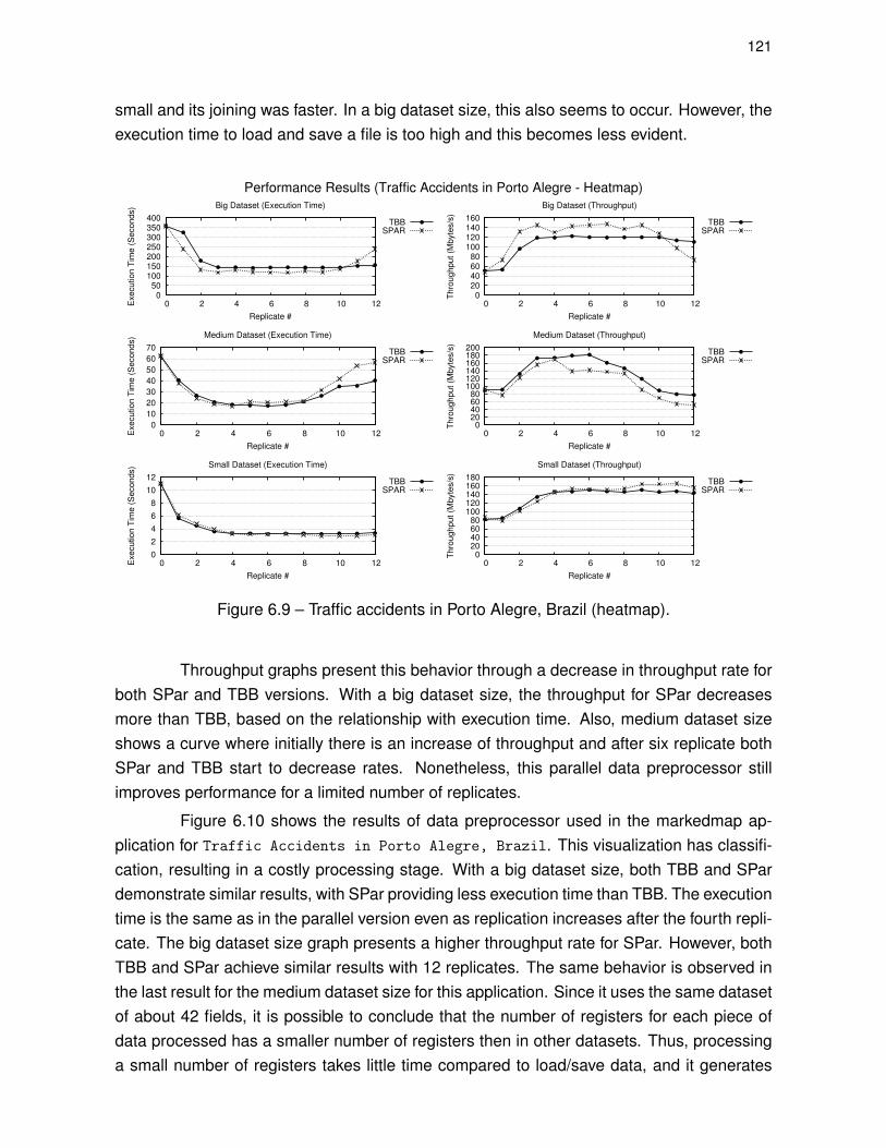
121

small and its joining was faster. In a big dataset size, this also seems to occur. However, theexecution time to load and save a file is too high and this becomes less evident.

Performance Results (Traffic Accidents in Porto Alegre - Heatmap)

0 50

100 150 200 250 300 350 400

0 2 4 6 8 10 12Execution T

ime (

Seconds)

Replicate #

Big Dataset (Execution Time)

TBBSPAR

0 20 40 60 80

100 120 140 160

0 2 4 6 8 10 12

Thro

ughput

(Mbyte

s/s

)

Replicate #

Big Dataset (Throughput)

TBBSPAR

0

10

20

30

40

50

60

70

0 2 4 6 8 10 12Exe

cu

tio

n T

ime (

Seconds)

Replicate #

Medium Dataset (Execution Time)

TBBSPAR

0 20 40 60 80

100 120 140 160 180 200

0 2 4 6 8 10 12

Th

rou

ghput

(Mbyte

s/s

)Replicate #

Medium Dataset (Throughput)

TBBSPAR

0

2

4

6

8

10

12

0 2 4 6 8 10 12Exe

cu

tio

n T

ime

(S

eco

nd

s)

Replicate #

Small Dataset (Execution Time)

TBBSPAR

0 20 40 60 80

100 120 140 160 180

0 2 4 6 8 10 12

Th

rou

gh

pu

t (M

byte

s/s

)

Replicate #

Small Dataset (Throughput)

TBBSPAR

Figure 6.9 – Traffic accidents in Porto Alegre, Brazil (heatmap).

Throughput graphs present this behavior through a decrease in throughput rate forboth SPar and TBB versions. With a big dataset size, the throughput for SPar decreasesmore than TBB, based on the relationship with execution time. Also, medium dataset sizeshows a curve where initially there is an increase of throughput and after six replicate bothSPar and TBB start to decrease rates. Nonetheless, this parallel data preprocessor stillimproves performance for a limited number of replicates.

Figure 6.10 shows the results of data preprocessor used in the markedmap ap-plication for Traffic Accidents in Porto Alegre, Brazil. This visualization has classifi-cation, resulting in a costly processing stage. With a big dataset size, both TBB and SPardemonstrate similar results, with SPar providing less execution time than TBB. The executiontime is the same as in the parallel version even as replication increases after the fourth repli-cate. The big dataset size graph presents a higher throughput rate for SPar. However, bothTBB and SPar achieve similar results with 12 replicates. The same behavior is observed inthe last result for the medium dataset size for this application. Since it uses the same datasetof about 42 fields, it is possible to conclude that the number of registers for each piece ofdata processed has a smaller number of registers then in other datasets. Thus, processinga small number of registers takes little time compared to load/save data, and it generates

122

a bottleneck in the output saving process. With the small dataset size, this is not observeddue to the small amount of data, which is processed quickly in both loading and saving data.

Performance Results (Traffic Accidents in Porto Alegre - Markedmap)

0 50

100 150 200 250 300 350 400 450

0 2 4 6 8 10 12Execution T

ime (

Seconds)

Replicate #

Big Dataset (Execution Time)

TBBSPAR

0 20 40 60 80

100 120 140 160

0 2 4 6 8 10 12

Thro

ughput

(Mbyte

s/s

)

Replicate #

Big Dataset (Throughput)

TBBSPAR

0

10

20

30

40

50

60

70

0 2 4 6 8 10 12Exe

cution T

ime (

Seconds)

Replicate #

Medium Dataset (Execution Time)

TBBSPAR

0 20 40 60 80

100 120 140 160 180

0 2 4 6 8 10 12

Thro

ughput

(Mbyte

s/s

)

Replicate #

Medium Dataset (Throughput)

TBBSPAR

0

2

4

6

8

10

12

0 2 4 6 8 10 12Exe

cu

tio

n T

ime

(S

eco

nd

s)

Replicate #

Small Dataset (Execution Time)

TBBSPAR

0 20 40 60 80

100 120 140 160

0 2 4 6 8 10 12

Th

rou

gh

pu

t (M

byte

s/s

)

Replicate #

Small Dataset (Throughput)

TBBSPAR

Figure 6.10 – Traffic accidents in Porto Alegre, Brazil with classification (marked map).

The throughput of both small and medium dataset sizes presented favorable resultsfor TBB. With a medium dataset size, SPar had an execution time close to TBB, but afterfour replicates, it started to decrease. TBB throughput also decreased but presented higherrates. With a small dataset size, both interfaces have a similar rates, keeping the throughputapproximately 140 Mbytes/s.

Figure 6.11 shows the last performed executions of the data preprocessor of FlickrPhotos Taken in 2014 Classified by Used Camera Brand. This application used a markedmap visualization type, applying filtering and classifying. Its results for execution time aresimilar to the first analyzed application. With a big dataset size, SPar presented a lowerexecution than TBB. It also had throughput higher than TBB. Medium dataset size initiallypresented execution time values to SPar and after five replicates this changes, but there isa small increase rate as replication occurs. This is highlighted in throughput results, whererates start to decrease after replicate 5 for SPar and 6 for TBB. Finally, small dataset sizepresents better results when compared with sequential time, there is not significant increasein execution time after four replications.

Considering that GMaVis data preprocessor requires sequential reading and sav-ing of data directly to the disk, results presented good execution times and speed up forthe parallel version of the data preprocessor. This answers research question two (Q2) by

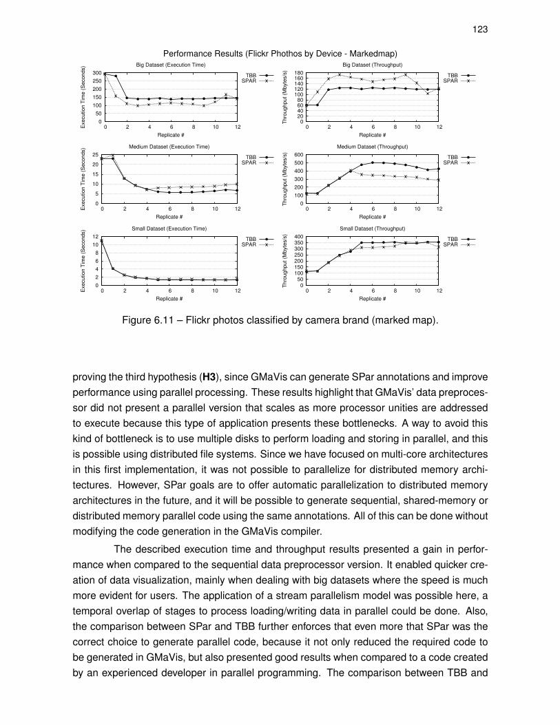
123

Performance Results (Flickr Phothos by Device - Markedmap)

0

50

100

150

200

250

300

0 2 4 6 8 10 12Execution T

ime (

Seconds)

Replicate #

Big Dataset (Execution Time)

TBBSPAR

0 20 40 60 80

100 120 140 160 180

0 2 4 6 8 10 12

Thro

ughput

(Mbyte

s/s

)

Replicate #

Big Dataset (Throughput)

TBBSPAR

0

5

10

15

20

25

0 2 4 6 8 10 12Execution T

ime (

Seconds)

Replicate #

Medium Dataset (Execution Time)

TBBSPAR

0

100

200

300

400

500

600

0 2 4 6 8 10 12

Thro

ughput

(Mbyte

s/s

)

Replicate #

Medium Dataset (Throughput)

TBBSPAR

0

2

4

6

8

10

12

0 2 4 6 8 10 12Exe

cu

tio

n T

ime (

Seconds)

Replicate #

Small Dataset (Execution Time)

TBBSPAR

0 50

100 150 200 250 300 350 400

0 2 4 6 8 10 12

Th

rou

gh

pu

t (M

byte

s/s

)

Replicate #

Small Dataset (Throughput)

TBBSPAR

Figure 6.11 – Flickr photos classified by camera brand (marked map).

proving the third hypothesis (H3), since GMaVis can generate SPar annotations and improveperformance using parallel processing. These results highlight that GMaVis’ data preproces-sor did not present a parallel version that scales as more processor unities are addressedto execute because this type of application presents these bottlenecks. A way to avoid thiskind of bottleneck is to use multiple disks to perform loading and storing in parallel, and thisis possible using distributed file systems. Since we have focused on multi-core architecturesin this first implementation, it was not possible to parallelize for distributed memory archi-tectures. However, SPar goals are to offer automatic parallelization to distributed memoryarchitectures in the future, and it will be possible to generate sequential, shared-memory ordistributed memory parallel code using the same annotations. All of this can be done withoutmodifying the code generation in the GMaVis compiler.

The described execution time and throughput results presented a gain in perfor-mance when compared to the sequential data preprocessor version. It enabled quicker cre-ation of data visualization, mainly when dealing with big datasets where the speed is muchmore evident for users. The application of a stream parallelism model was possible here, atemporal overlap of stages to process loading/writing data in parallel could be done. Also,the comparison between SPar and TBB further enforces that even more that SPar was thecorrect choice to generate parallel code, because it not only reduced the required code tobe generated in GMaVis, but also presented good results when compared to a code createdby an experienced developer in parallel programming. The comparison between TBB and

124

SPar also proves hypothesis four (H4), showing that both generation and execution for SParimproves and facilitates the code generation and processing in GMaVis.

125

7. CONCLUSIONS

In this work, we proposed GMaVis, a DSL (domain-specific language) for geospa-tial data visualization creation to offer features for users to create data visualizations withonly a few lines of code by using a high-level description language to specify the visualiza-tion. We also provides a compiler that receives GMaVis source code and data as input togenerate the data visualization automatically. Both GMaVis and the compiler were describedin this work, including grammar, compilation phases, internal processing, and parallel codegeneration.

This DSL used SPar to parallelize the data preprocessor since it provides an easyway to implement parallel code both in a parallel or sequential way by just changing a com-piler argument. It enabled the generation of the same code to be used in both architectures,whereas other interfaces would have required the implementation of two different code gen-erations. Furthermore, this DSL generates parallel code to run on multi-core systems. Itaims to generate parallel code to run in distributed memory systems, however, shared mem-ory systems are more accessible for domain users than a cluster with multiple computers.Therefore, to create this DSL and enable its first use, we initially focused on multi-core sys-tems.

Also, two research questions were formulated in order to evaluate this DSL in re-spect to code usability and performance. In order to answer these questions, two experi-ments for analyzing programming effort and data processing execution time were performed.Furthermore, both research questions, methodology and results are briefly described bellow.

Q1 - Is it possible to create a DSL (GMAVIS) to reduce the programming effortfor creating geospatial visualization?

To answer Q1, two evaluations of GMaVis were performed and analyzed. First theprogramming effort estimation data produced by SLOCCount was used to compare the ef-fort required for creating a information visualization when using GMaVis to other librariessuch as Google Maps API, OpenLayers, and Leaflet. Results demonstrated that even whenproviding the abstraction of complexities in the data pre-processing phase and totally par-allel programming abstraction, GMaVis could reduce the programming effort and cost re-quired to implement the three supported data visualizations (clusteredmap, heatmap, andmarkedmap). Furthermore, it measured an application that could perform data process-ing for the compared libraries, to estimate the effort required if users were to implement it.Thus, it is possible to confirm that GMaVis can reduce not only the programming effort butalso the cost of development for creating geospatial data visualizations (i.e., markedmaps,clusteredmaps and heatmaps).

Q2 - Can the parallel code generated by this DSL speed up the data process-ing of raw geospatial data?

126

In respect to Q2, an evaluation in a parallel data preprocessor that was generatedin the GMaVis compiler using SPar. This evaluation used execution time and throughput ofsix applications parallelized with SPar using the GMaVis compiler and manually with TBB,using three data loads and many configurations of parallel processing replication. The objec-tive was to verify if it has better performance in parallel execution and to analyze if GMaVisgenerates the correct annotations to SPar in order to have good performance. Thus, wecompared GMaVis generated code with SPar annotations to the TBB manually parallelizedversion of the data preprocessor. Results demonstrated that both versions increased per-formance through decreasing the execution time when compared to the sequential version.Also, both SPar and TBB offered an increase in throughput for the data preprocessor, en-abling the processing of more data in less time compared to the sequential version.

7.1 Contributions

This work contributes by providing a domain-specific language that abstracts com-plexities in the whole visualization creation workflow, since it includes the data pre-processingphase features and does not require users to handle data manually. Also, the proposed DSLabstracts all parallelism. Users do not need to think about computer architecture for parallelprocessing, interfaces, communication, synchronization or any other parallel programmingcomplexities. They instead focus on the description language to express the visualizationusing their data.

Another contribution of this work is to enable users to process huge files in multi-core systems when implementing a visualization. This makes it easier for users that haveto create a visualization of datasets that have large files, bigger than available memory.Through a study of different selected algorithms, it was possible to implement an efficientdata search in unsorted data and use an effective memory management by splitting data.

Also, estimations prove that this DSL enables users to create data visualization withless development effort, time and cost. This is possible because GMaVis has a simple gram-mar with few declarations to specify only required information to generate the visualization.Furthermore, this grammar is recognized by a built-in compiler. This compiler transformsGMaVis’ source code and data into the final visualization, creating all of the visualizationsteps automatically and performing data processing in parallel through the use of SPar.Moreover, the parallel code generated in GMaVis to SPar demonstrated execution time andthroughput results close to those manually implemented in a TBB version of a parallel datapreprocessor. This shows that GMaVis also can efficiently generate the annotations for SParduring data preprocessor generation.

127

7.2 Identified Limitations

During this DSL creation and evaluation, some limitations were identified. The firstlimitation is due to the system architecture used to parallelize the code. Shared memoryarchitectures have a bottleneck when reading data from disk, which requires sequentialprocessing. This step in data processing made it difficult to parallelize and achieve goodperformance results compared to the sequential version. This is because the data mustbe read from the disk, processed and then written again. Both the initial and final stepis performed sequentially. However, the parallelism to shared memory architectures werechosen because currently most computers have this architecture and it is more accessiblethan a cluster or grid. Thus, the first version of GMaVis was implemented targeting thesetypes of architectures. In future work, the plan is to improve this DSL to perform in distributedmemory architectures.

Since GMaVis is an external DSL that has a high-level description language, itoffers low expressiveness. This is because to offer a higher level of abstraction, it is requiredto keep some features hidden from users that allow changing some visualization details,such as colors, icons, and specific sizes. However, GMaVis generates the visualizationwith a readable code, and it enables experienced users to change the final visualization ifneeded.

This DSL has focused in geospatial data visualizations. However, data analysismay require the use of different visualization types/techniques to achieve its objective. Cur-rently, GMaVis only offers three visualization types. If users need to implement another typeof visualization, it will not be possible with this DSL. However, the insertion and support ofother visualization types in is planned for the future, using geospatial data.

The data preprocessor in GMaVis only supports non-hierarchical data files like CSVor tab separated files. Hierarchical data files such as JSON or XML were not supported yet.However, the creation of a pre-parser for these files are planned for future work. Also, it ispossible to use or convert a hierarchical into a non-hierarchical data file.

7.3 Future Work

For future work, this high-level interface will be expanded to offer the most com-monly used visualization types for big data analysis and abstract complexities throughoutthe whole visualization creation workflow. Thus, many domain users may use this DSL. Thiswill support a set of visualization types which will facilitate users to create and modify theirvisualization by simply changing a few lines of source code. These visualizations may beinserted as modules in the DSL’s compiler. Also, it is possible to use other libraries or gen-

128

erate them from scratch, and use parallel processing in data to visual mappings phase foroffering 3D visualizations using GPU or multi-core processing.

Also, data declarations can be extended in this interface to offer smart classifica-tions and data selection through the use of machine learning and data mining algorithms.The main challenge here is to apply data classification in pieces of data, since GMaVis datapreprocessor splits data to process. Moreover, extending this language grammar is possibleby adding more logical operators and filtering options, data values and enabling users tospecify data directly from the web.

Furthermore, it is possible to improve this DSL through the use of distributed mem-ory architectures for better performance and execution time in data processing. This alsoincludes the possibility of using the MapReduce model, since it can provide distributed dataprocessing and has been used in other projects [MR14, Gup15, RS14, LLA14] with similarobjectives. After this implementation, it will be possible to create a smart scheduler to verifythe best target architecture (distributed or shared memory) to process input data in parallel.This choice will be made based on variables such as, input size, filters, classification andother issues that may influence execution time.

129

REFERENCES

[AGLF15a] Adornes, D.; Griebler, D.; Ledur, C.; Fernandes, L. G. “A Unified MapReduceDomain-Specific Language for Distributed and Shared Memory Architectures”.In: Proceedings of the 27th International Conference on Software Engineering& Knowledge Engineering, 2015, pp. 6.

[AGLF15b] Adornes, D.; Griebler, D.; Ledur, C.; Fernandes, L. G. “Coding Productivity inMapReduce Applications for Distributed and Shared Memory Architectures”,International Journal of Software Engineering and Knowledge Engineering,2015, pp. 4.

[ART10] Aldinucci, M.; Ruggieri, S.; Torquati, M. “Porting Decision Tree Algorithmsto Multicore Using FastFlow”. In: Proceedings of the Machine Learning andKnowledge Discovery in Databases, 2010, pp. 7–23.

[ASU06] Aho, A. V.; Sethi, R.; Ullman, J. D. “Compilers: Principles, Techniques,and Tools (Second Edition)”. Boston, MA, USA: Addison-Wesley LongmanPublishing Co., Inc., 2006, 1000p.

[Bar15] Barney, B. “Introduction to Parallel Computing”. Source: https://computing.llnl.gov/tutorials/parallel_comp/, 2014 (accessed October 11, 2015).

[Boe81] Boehm, B. W. “Software Engineering Economics”. Upper Saddle River, NJ,USA: Prentice Hall PTR, 1981, 767p.

[CCQ+er] Choi, H.; Choi, W.; Quan, T.; Hildebrand, D. G.; Pfister, H.; Jeong, W.-K.“Vivaldi: A Domain-Specific Language for Volume Processing and Visualizationon Distributed Heterogeneous Systems”, IEEE Transactions on Visualizationand Computer Graphics, vol. 20–12, 2014 December, pp. 2407–2416.

[CGS97] Culler, D. E.; Gupta, A.; Singh, J. P. “Parallel Computer Architecture: AHardware/Software Approach”. San Francisco, CA, USA: Morgan KaufmannPublishers Inc., 1997, 1056p.

[CJvdP07] Chapman, B.; Jost, G.; van der Pas, R. “Using OpenMP: Portable SharedMemory Parallel Programming (Scientific and Engineering Computation)”.London, England: The MIT Press, 2007, 23p.

[CKR+12] Chiw, C.; Kindlmann, G.; Reppy, J.; Samuels, L.; Seltzer, N. “Diderot: AParallel DSL for Image Analysis and Visualization”. In: Proceedings of the ACMSIGPLAN Conference on Programming Language Design and Implementation,2012, pp. 111–120.

130

[CL11] Cormen, T. H.; Leiserson, C. E. “Introduction to Algorithms”. London, England:The MIT Press, 2011, 1312p.

[CMS99] Card, S. K.; Mackinlay, J. D.; Shneiderman, B. “Readings in InformationVisualization: Using Vision to Think”. San Francisco, CA, USA: MorganKaufmann Publishers Inc., 1999, 712p.

[DSR11] Devi, S. G.; Selvam, K.; Rajagopalan, S. P. “An Abstract to Calculate Big OFactors of Time and Space Complexity of Machine Code”. In: Proceedings ofthe International Conference on Sustainable Energy and Intelligent Systems,2011, pp. 844–847.

[Fow10] Fowler, M. “Domain-Specific Languages”. Massachusetts, USA: PearsonEducation, 2010, 640p.

[GAF14] Griebler, D.; Adornes, D.; Fernandes, L. G. “Performance and UsabilityEvaluation of a Pattern-Oriented Parallel Programming Interface for Multi-Core Architectures”. In: Proceedings of the 26th International Conference onSoftware Engineering & Knowledge Engineering, 2014, pp. 25–30.

[Gao15a] Gao, L. “Bison Tutorial”. Source: http://alumni.cs.ucr.edu/~lgao/teaching/bison.html, January 2015 (accessed November 09, 2015).

[Gao15b] Gao, L. “FLEX Tutorial”. Source: http://alumni.cs.ucr.edu/~lgao/teaching/flex.html, January 2015 (accessed November 26, 2015).

[Gha07] Ghanbari, M. “Visualization Overview”. In: Proceedings of the SoutheasternSymposium on System Theory, 2007, pp. 115–119.

[Gho10] Ghosh, D. “DSLs in Action”. Greenwich, CT, USA: Manning Publications Co.,2010, 376p.

[Gri16] Griebler, D. “Domain-Specific Language & Support Tool for High-Level StreamParallelism”, Ph.D. Thesis, Faculdade de Informática - PPGCC - PUCRS, PortoAlegre, Brazil, 2016, 200p.

[Gup15] Gupta, A. “Big Data Analysis Using Computational Intelligence and Hadoop:A Study”. In: Proceedings of the International Conference on Computing forSustainable Global Development, 2015, pp. 1397–1401.

[Gus11] Gustafson, J. L. “Little’s Law”. In: Encyclopedia of Parallel Computing, Padua,D. (Editor), Springer US, 2011, pp. 1038–1041.

[HFB05] Hertz, M.; Feng, Y.; Berger, E. D. “Garbage Collection Without Paging”. In:Proceedings of the ACM SIGPLAN Conference on Programming LanguageDesign and Implementation, 2005, pp. 143–153.

131

[Hil04] Hill, E. “First Course: Data Structures and Algorithms Using Java”. iUniverse,2004, 107p.

[HWCP15] Hasan, M.; Wolfgang, J.; Chen, G.; Pfister, H. “Shadie: A Domain-SpecificLanguage for Volume Visualization”. Source: http://miloshasan.net/Shadie/shadie.pdf, 2010 (accessed December 15, 2015).

[INT15] INTEL. “Intel Software Network (Official page of Intel)”. Source:http://software.intel.com/en-us/articles/intel-parallel-studio-home>, June 2015(accessed December 02, 2015).

[KCS+16] Kindlmann, G.; Chiw, C.; Seltzer, N.; Samuels, L.; Reppy, J. “Diderot: aDomain-Specific Language for Portable Parallel Scientific Visualization andImage Analysis”, IEEE Transactions on Visualization and Computer Graphics,vol. 22–1, January 2016, pp. 867–876.

[KEH+09] Klein, G.; Elphinstone, K.; Heiser, G.; Andronick, J.; Cock, D.; Derrin, P.;Elkaduwe, D.; Engelhardt, K.; Kolanski, R.; Norrish, M.; Sewell, T.; Tuch, H.;Winwood, S. “SeL4: Formal Verification of an OS Kernel”. In: Proceedingsof the ACM SIGOPS Symposium on Operating Systems Principles, 2009, pp.207–220.

[Knu76] Knuth, D. E. “Big Omicron and Big Omega and Big Theta”, SIGACT News,vol. 8, April 1976, pp. 18–24.

[Kri09] Krithivasan, K. “Introduction to Formal Languages, Automata Theory andComputation”. India: Pearson Education, 2009, 436p.

[Lea15] Leaflet. “Leaflet Documentation”. Source: http://leafletjs.com/reference.html,June 2015 (accessed May 2, 2015).

[Lei09] Leiserson, C. E. “The Cilk++ Concurrency Platform”. In: Proceedings of theAnnual Design Automation Conference, 2009, pp. 522–527.

[LGMF15] Ledur, C.; Griebler, D.; Manssuor, I.; Fernandes, L. G. “Towards a Domain-Specific Language for Geospatial Data Visualization Maps with Big Data Sets”.In: Proceedings of the ACS/IEEE International Conference on ComputerSystems and Applications, 2015, pp. 8.

[LLA14] Liu, J.; Liu, F.; Ansari, N. “Monitoring and Analyzing Big Traffic Data of a Large-Scale Cellular Network with Hadoop”, IEEE Network, vol. 28–4, July 2014, pp.32–39.

[LRCS14] Li, K.; Reichenbach, C.; Csallner, C.; Smaragdakis, Y. “Residual Investigation:Predictive and Precise Bug Detection”, ACM Transactions on SoftwareEngineering and Methodology, vol. 24–2, December 2014, pp. 7:1–7:32.

132

[LV15] Lyman, P.; Varian, H. “How Much Information?” Source: http://groups.ischool.berkeley.edu/archive/how-much-info-2003/, October 2004 (accessed October16, 2015).

[MCB+11] Manyika, J.; Chui, M.; Brown, B.; Bughin, J.; Dobbs, R.; Roxburgh, C.;Byers, A. H. “Big Data: The Next Frontier for Innovation, Competition, andProductivity”, Technical Report, McKinsey Global Institute, 2011, 156p.

[MHS05] Mernik, M.; Heering, J.; Sloane, A. M. “When and How to DevelopDomain-Specific Languages”, ACM Computing Surveys (CSUR), vol. 37–4,December 2005, pp. 316–344.

[MR14] Manikandan, S. G.; Ravi, S. “Big Data Analysis Using Apache Hadoop”. In:Proceedings of the International Conference on IT Convergence and Security,2014, pp. 1–4.

[MSM04] Mattson, T.; Sanders, B.; Massingill, B. “Patterns for Parallel Programming”.Boston, EUA: Addison-Wesley Professional, 2004, 384p.

[MTAB15] Meyerovich, L. A.; Torok, M. E.; Atkinson, E.; Bodík, R. “Superconductor: ALanguage for Big Data Visualization”. Source: https://engineering.purdue.edu/~milind/lashc13/meyerovich-superconductor.pdf, February 2013 (accessedDecember 17, 2015).

[NBF96] Nichols, B.; Buttlar, D.; Farrell, J. P. “Pthreads Programming”. Sebastopol, CA,USA: O’Reilly & Associates, Inc., 1996, 286p.

[Ope15] OpenLayers. “OpenLayers Documentation”. Source: http://openlayers.org/en/v3.6.0/doc/tutorials/introduction.html, June 2015 (accessed August 1, 2015).

[Pac11] Pacheco, P. “An Introduction to Parallel Programming”. San Francisco, CA,USA: Morgan Kaufmann Publishers Inc., 2011, 370p.

[RBGH14] Rautek, P.; Bruckner, S.; Groller, M.; Hadwiger, M. “ViSlang: A Systemfor Interpreted Domain-Specific Languages for Scientific Visualization”,IEEE Transactions on Visualization and Computer Graphics, vol. 20–12,December 2014, pp. 2388–2396.

[Rei07] Reinders, J. “Intel Threading Building Blocks: Outfitting C++ for Multi-CoreProcessor Parallelism”. Sebastopol, USA: O’Reilly and Associates, 2007,336p.

[RGBMA06] Robles, G.; Gonzalez-Barahona, J. M.; Michlmayr, M.; Amor, J. J. “MiningLarge Software Compilations over Time: Another Perspective of Software

133

Evolution”. In: Proceedings of the International Workshop on Mining SoftwareRepositories, 2006, pp. 3–9.

[RR13] Rauber, T.; Runger, G. “Parallel programming: For Multicore and ClusterSystems”. Bayreuth, Germany: Springer Berlin Heidelberg, 2013, 516p.

[RS14] Ramya, A.; Sivasankar, E. “Distributed Pattern Matching and DocumentAnalysis in Big Data Using Hadoop MapReduce Model”. In: Proceedings of theInternational Conference on Parallel, Distributed and Grid Computing, 2014,pp. 312–317.

[Rus08] Rust, K. “Using Little’s Law to Estimate Cycle Time and Cost”. In: Proceedingsof the 40th Conference on Winter Simulation, 2008, pp. 2223–2228.

[SET+09] Shinagawa, T.; Eiraku, H.; Tanimoto, K.; Omote, K.; Hasegawa, S.; Horie, T.;Hirano, M.; Kourai, K.; Oyama, Y.; Kawai, E.; Kono, K.; Chiba, S.; Shinjo,Y.; Kato, K. “BitVisor: A Thin Hypervisor for Enforcing I/O Device Security”.In: Proceedings of the ACM SIGPLAN/SIGOPS International Conference onVirtual Execution Environments, 2009, pp. 121–130.

[STM10] Siefers, J.; Tan, G.; Morrisett, G. “Robusta: Taming the Native Beastof the JVM”. In: Proceedings of the ACM Conference on Computer andCommunications Security, 2010, pp. 201–211.

[Sve10] Svennerberg, G. “Beginning Google Maps API 3”. Berkely, CA, USA: Apress,2010, 328p.

[TSF+15] Thomee, B.; Shamma, D. A.; Friedland, G.; Elizalde, B.; Ni, K.; Poland, D.;Borth, D.; Li, L. “The New Data and New Challenges in Multimedia Research”,CoRR arXiv eprint, vol. abs/1503.01817, 2015.

[VBD+13] Voelter, M.; Benz, S.; Dietrich, C.; Engelmann, B.; Helander, M.; Kats, L. C. L.;Visser, E.; Wachsmuth, G. “DSL Engineering - Designing, Implementing andUsing Domain-Specific Languages”. dslbook.org, 2013, 558p.

[vDKV00] van Deursen, A.; Klint, P.; Visser, J. “Domain-Specific Languages: AnAnnotated Bibliography”, ACM SIGPLAN Notices, vol. 35–6, June 2000, pp.26–36.

[VSJ+14] Vazou, N.; Seidel, E. L.; Jhala, R.; Vytiniotis, D.; Peyton-Jones, S. “RefinementTypes for Haskell”. In: Proceedings of the ACM SIGPLAN InternationalConference on Functional Programming, 2014, pp. 269–282.

[WGK10] Ward, M. O.; Grinstein, G.; Keim, D. “Interactive Data Visualization:Foundations, Techniques, and Applications”. Massachusetts, USA: CRCPress, 2010, 513p.

134

[Whe16] Wheeler, D. A. “SLOCCount Documentation”. Source: http://www.dwheeler.com/sloccount/, October 2015 (accessed January 11, 2016).

[WWA15] Wang, L.; Wang, G.; Alexander, C. A. “Big Data and Visualization: Methods,Challenges and Technology Progress”, Digital Technologies, vol. 1–1, 2015,pp. 33–38.

[ZCL13] Zhang, J.; Chen, Y.; Li, T. “Opportunities of Innovation under Challenges of BigData”. In: Proceedings of the International Conference on Fuzzy Systems andKnowledge Discovery, 2013, pp. 669–673.

[ZH13] Zhang, J.; Huang, M. L. “5Ws Model for Big Data Analysis and Visualization”.In: Proceedings of the International Conference on Computational Science andEngineering, 2013, pp. 1021–1028.

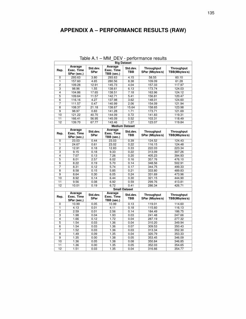
135

APPENDIX A – PERFORMANCE RESULTS (RAW)

Table A.1 – MM_DEV - performance resultsBig Dataset

Rep.Avarage

Exec. TimeSPar (sec.)

Std.dev.SPar

AvarageExec. TimeTBB (sec.)

Std.dev.TBB

ThroughputSPar (Mbytes/s)

ThroughputTBB(Mbytes/s)

0 293.63 3.80 293.63 4.15 58.55 60.101 157.60 4.65 280.56 8.38 109.09 61.282 109.28 12.91 145.73 4.04 157.33 117.973 98.96 1.55 138.61 6.13 173.74 124.034 104.86 17.65 138.51 7.18 163.96 124.125 109.64 11.57 142.71 5.41 156.81 120.476 116.16 4.27 137.98 3.62 148.01 124.607 111.57 0.47 140.99 2.06 154.09 121.948 108.37 21.18 138.67 15.64 158.65 123.989 98.97 0.83 141.28 1.71 173.71 121.6910 121.22 40.70 144.09 0.72 141.83 119.3111 166.41 56.95 145.09 0.52 103.31 118.4912 139.70 67.77 143.46 1.27 123.07 119.84

Medium Dataset

Rep.Avarage

Exec. TimeSPar (sec.)

Std.dev.SPar

AvarageExec. TimeTBB (sec.)

Std.dev.TBB

ThroughputSPar (Mbytes/s)

ThroughputTBB(Mbytes/s)

0 23.03 0.44 23.03 0.39 124.52 124.431 24.67 0.61 23.02 0.22 116.15 124.482 12.91 0.18 12.83 0.33 222.03 223.343 9.15 0.18 9.33 0.22 313.09 307.264 7.07 0.13 7.26 0.20 405.23 394.935 8.01 2.57 6.02 0.16 357.76 476.106 8.22 0.19 5.70 0.14 348.56 502.917 8.31 0.12 5.74 0.17 344.75 499.338 8.58 0.15 5.85 0.21 333.80 489.839 8.64 0.30 6.05 0.24 331.69 473.9610 8.92 0.14 6.44 0.30 321.15 444.9011 9.56 0.08 6.92 0.59 299.76 413.8112 10.01 0.19 6.72 0.41 286.34 426.71

Small Dataset

Rep.Avarage

Exec. TimeSPar (sec.)

Std.dev.SPar

AvarageExec. TimeTBB (sec.)

Std.dev.TBB

ThroughputSPar (Mbytes/s)

ThroughputTBB(Mbytes/s)

0 10.99 0.05 10.99 0.13 119.01 114.601 4.13 0.01 4.11 0.18 115.60 116.132 2.59 0.01 2.56 0.14 184.49 186.753 1.98 0.04 1.93 0.03 241.48 247.664 1.66 0.12 1.72 0.04 287.19 277.325 1.54 0.03 1.36 0.04 310.20 349.946 1.54 0.03 1.36 0.07 309.53 350.437 1.52 0.03 1.36 0.03 313.34 352.308 1.49 0.09 1.35 0.04 320.79 353.339 1.35 0.00 1.38 0.05 353.45 346.0910 1.36 0.05 1.38 0.08 350.84 346.8511 1.36 0.00 1.35 0.05 352.03 354.6512 1.51 0.03 1.35 0.04 316.66 354.77

136

Table A.2 – MM_ACID - performance resultsBig Dataset

Rep.Avarage

Exec. TimeSPar (sec.)

Std.dev.SPar

AvarageExec. TimeTBB (sec.)

Std.dev.TBB

ThroughputSPar (Mbytes/s)

ThroughputTBB(Mbytes/s)

0 427.16 1.47 427.16 20.11 40.44 42.601 300.39 4.28 384.45 15.87 57.50 44.932 158.85 2.69 210.48 3.90 108.74 82.063 118.71 1.77 159.03 2.76 145.51 108.614 135.47 8.28 149.56 1.76 127.50 115.495 118.35 7.50 144.45 2.45 145.95 119.576 120.38 11.32 146.36 1.89 143.49 118.017 117.88 1.20 147.20 2.89 146.53 117.348 128.91 6.39 148.34 3.35 133.99 116.449 119.48 0.55 149.35 6.98 144.57 115.6510 135.21 103.48 154.28 10.06 127.75 111.9511 165.05 164.75 155.69 19.17 104.65 110.9412 159.51 102.94 168.61 12.56 108.29 102.44

Medium Dataset

Rep.Avarage

Exec. TimeSPar (sec.)

Std.dev.SPar

AvarageExec. TimeTBB (sec.)

Std.dev.TBB

ThroughputSPar (Mbytes/s)

ThroughputTBB(Mbytes/s)

0 62.48 0.70 40.70 0.41 70.90 70.731 48.31 0.34 40.58 1.12 59.59 70.932 28.52 2.57 26.57 2.50 100.93 108.363 22.13 1.06 20.59 2.02 130.07 139.844 19.14 0.64 18.35 1.07 150.44 156.905 21.37 1.02 17.66 1.21 134.72 163.046 21.33 0.43 17.40 0.64 134.98 165.417 22.22 1.21 18.14 0.50 129.56 158.678 22.93 1.72 21.11 0.94 125.56 136.399 37.34 5.32 26.43 4.84 77.09 108.9310 43.03 7.75 34.84 5.89 66.91 82.6411 51.26 6.03 35.38 6.40 56.16 81.3712 58.06 4.13 40.20 3.48 49.58 71.61

Small Dataset

Rep.Avarage

Exec. TimeSPar (sec.)

Std.dev.SPar

AvarageExec. TimeTBB (sec.)

Std.dev.TBB

ThroughputSPar (Mbytes/s)

ThroughputTBB(Mbytes/s)

0 10.99 0.40 7.46 0.39 66.78 64.331 7.94 0.07 6.99 0.02 60.45 68.612 5.83 0.33 5.16 0.49 82.32 93.073 4.24 0.38 4.21 0.45 113.06 114.014 4.01 0.09 3.87 0.29 119.58 123.845 3.48 0.05 3.70 0.19 137.71 129.686 3.45 0.07 3.48 0.23 139.16 137.837 3.56 0.03 3.55 0.20 134.96 135.158 3.46 0.11 3.54 0.33 138.61 135.519 3.29 0.04 3.41 0.21 145.90 140.7410 3.31 0.05 3.58 0.16 145.02 134.1011 3.28 0.06 3.45 0.15 146.50 138.9612 3.65 0.06 3.43 0.23 131.27 139.80

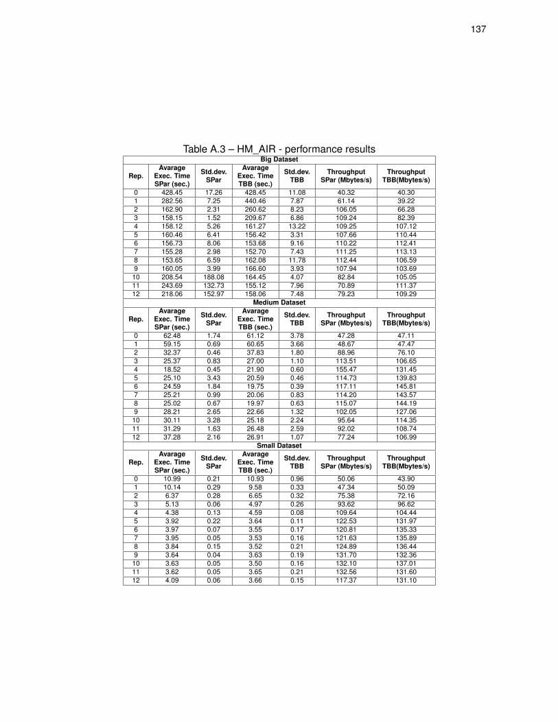
137

Table A.3 – HM_AIR - performance resultsBig Dataset

Rep.Avarage

Exec. TimeSPar (sec.)

Std.dev.SPar

AvarageExec. TimeTBB (sec.)

Std.dev.TBB

ThroughputSPar (Mbytes/s)

ThroughputTBB(Mbytes/s)

0 428.45 17.26 428.45 11.08 40.32 40.301 282.56 7.25 440.46 7.87 61.14 39.222 162.90 2.31 260.62 8.23 106.05 66.283 158.15 1.52 209.67 6.86 109.24 82.394 158.12 5.26 161.27 13.22 109.25 107.125 160.46 6.41 156.42 3.31 107.66 110.446 156.73 8.06 153.68 9.16 110.22 112.417 155.28 2.98 152.70 7.43 111.25 113.138 153.65 6.59 162.08 11.78 112.44 106.599 160.05 3.99 166.60 3.93 107.94 103.6910 208.54 188.08 164.45 4.07 82.84 105.0511 243.69 132.73 155.12 7.96 70.89 111.3712 218.06 152.97 158.06 7.48 79.23 109.29

Medium Dataset

Rep.Avarage

Exec. TimeSPar (sec.)

Std.dev.SPar

AvarageExec. TimeTBB (sec.)

Std.dev.TBB

ThroughputSPar (Mbytes/s)

ThroughputTBB(Mbytes/s)

0 62.48 1.74 61.12 3.78 47.28 47.111 59.15 0.69 60.65 3.66 48.67 47.472 32.37 0.46 37.83 1.80 88.96 76.103 25.37 0.83 27.00 1.10 113.51 106.654 18.52 0.45 21.90 0.60 155.47 131.455 25.10 3.43 20.59 0.46 114.73 139.836 24.59 1.84 19.75 0.39 117.11 145.817 25.21 0.99 20.06 0.83 114.20 143.578 25.02 0.67 19.97 0.63 115.07 144.199 28.21 2.65 22.66 1.32 102.05 127.0610 30.11 3.28 25.18 2.24 95.64 114.3511 31.29 1.63 26.48 2.59 92.02 108.7412 37.28 2.16 26.91 1.07 77.24 106.99

Small Dataset

Rep.Avarage

Exec. TimeSPar (sec.)

Std.dev.SPar

AvarageExec. TimeTBB (sec.)

Std.dev.TBB

ThroughputSPar (Mbytes/s)

ThroughputTBB(Mbytes/s)

0 10.99 0.21 10.93 0.96 50.06 43.901 10.14 0.29 9.58 0.33 47.34 50.092 6.37 0.28 6.65 0.32 75.38 72.163 5.13 0.06 4.97 0.26 93.62 96.624 4.38 0.13 4.59 0.08 109.64 104.445 3.92 0.22 3.64 0.11 122.53 131.976 3.97 0.07 3.55 0.17 120.81 135.337 3.95 0.05 3.53 0.16 121.63 135.898 3.84 0.15 3.52 0.21 124.89 136.449 3.64 0.04 3.63 0.19 131.70 132.3610 3.63 0.05 3.50 0.16 132.10 137.0111 3.62 0.05 3.65 0.21 132.56 131.6012 4.09 0.06 3.66 0.15 117.37 131.10

138

Table A.4 – HM_AC - performance resultsBig Dataset

Rep.Avarage

Exec. TimeSPar (sec.)

Std.dev.SPar

AvarageExec. TimeTBB (sec.)

Std.dev.TBB

ThroughputSPar (Mbytes/s)

ThroughputTBB(Mbytes/s)

0 358.85 1.71 358.85 16.69 48.13 50.671 238.42 4.35 325.27 7.85 72.45 53.102 130.90 5.55 179.20 3.81 131.96 96.393 118.41 6.85 145.02 3.14 145.88 119.104 132.47 8.37 144.71 3.82 130.39 119.365 120.45 11.97 141.07 3.27 143.40 122.446 118.55 2.99 143.58 2.65 145.70 120.307 117.24 1.47 144.63 0.42 147.33 119.428 125.85 8.39 144.00 0.34 137.25 119.949 118.71 1.22 143.66 0.21 145.50 120.2310 134.84 118.68 143.62 4.32 128.10 120.2611 176.93 96.78 151.95 13.98 97.62 113.6712 238.72 221.01 156.42 12.38 72.36 110.42

Medium Dataset

Rep.Avarage

Exec. TimeSPar (sec.)

Std.dev.SPar

AvarageExec. TimeTBB (sec.)

Std.dev.TBB

ThroughputSPar (Mbytes/s)

ThroughputTBB(Mbytes/s)

0 62.48 7.98 62.48 7.98 90.76 89.891 37.86 0.18 31.61 0.29 76.04 91.062 23.73 1.78 21.81 1.69 121.30 131.973 18.58 1.34 16.67 1.16 154.96 172.714 16.89 0.56 16.60 0.85 170.42 173.455 20.68 1.28 16.04 0.72 139.21 179.486 20.33 0.67 15.85 0.83 141.60 181.677 21.00 0.65 17.92 1.11 137.12 160.678 21.54 0.67 19.68 1.52 133.66 146.259 31.42 4.62 24.14 2.32 91.62 119.2810 41.39 7.82 32.30 4.78 69.56 89.1211 53.39 6.68 36.16 5.49 53.92 79.6112 56.48 7.35 37.09 8.48 50.97 77.61

Small Dataset

Rep.Avarage

Exec. TimeSPar (sec.)

Std.dev.SPar

AvarageExec. TimeTBB (sec.)

Std.dev.TBB

ThroughputSPar (Mbytes/s)

ThroughputTBB(Mbytes/s)

0 10.99 1.29 5.85 1.51 86.56 82.011 6.13 0.05 5.64 0.17 78.23 85.072 4.76 0.06 4.49 0.20 100.82 106.863 3.89 0.11 3.58 0.27 123.30 133.984 3.30 0.07 3.29 0.16 145.27 145.925 3.15 0.49 3.27 0.22 152.18 146.666 3.16 0.04 3.18 0.18 151.74 150.827 3.18 0.04 3.26 0.16 150.87 147.308 3.12 0.13 3.28 0.21 153.72 146.409 2.92 0.04 3.19 0.24 164.07 150.6110 2.92 0.02 3.29 0.22 164.09 145.8911 2.90 0.04 3.26 0.29 165.72 147.1712 3.09 0.03 3.33 0.18 155.26 143.94

139

Table A.5 – CM_CP - performance resultsBig Dataset

Rep.Avarage

Exec. TimeSPar (sec.)

Std.dev.SPar

AvarageExec. TimeTBB (sec.)

Std.dev.TBB

ThroughputSPar (Mbytes/s)

ThroughputTBB(Mbytes/s)

0 293.41 5.56 293.41 11.99 58.60 61.501 154.86 3.52 272.94 7.15 111.02 62.992 104.53 8.80 146.28 3.99 164.47 117.533 99.34 2.41 137.80 5.97 173.06 124.764 103.12 12.88 135.97 4.56 166.72 126.445 105.30 14.46 141.44 5.47 163.27 121.556 109.24 5.05 137.47 4.08 157.38 125.067 111.37 1.76 139.60 1.32 154.38 123.158 95.95 12.29 138.48 0.39 179.18 124.159 98.65 0.93 140.94 0.81 174.28 121.9810 115.37 14.69 143.98 0.76 149.02 119.4111 139.11 50.30 144.84 3.16 123.59 118.7012 123.96 12.31 143.36 1.29 138.70 119.92

Medium Dataset

Rep.Avarage

Exec. TimeSPar (sec.)

Std.dev.SPar

AvarageExec. TimeTBB (sec.)

Std.dev.TBB

ThroughputSPar (Mbytes/s)

ThroughputTBB(Mbytes/s)

0 23.47 4.83 23.47 7.53 124.92 122.081 24.56 0.52 23.05 0.43 116.69 124.322 12.91 0.18 12.68 0.34 221.95 225.953 9.18 0.27 9.28 0.15 312.02 308.644 7.01 0.13 7.20 0.16 408.89 397.865 8.16 4.98 6.00 0.13 351.12 477.446 8.15 0.23 5.75 0.22 351.47 498.607 8.34 0.12 5.77 0.23 343.62 496.328 8.67 0.16 5.80 0.18 330.60 494.179 8.82 0.38 6.11 0.20 324.81 468.6310 8.95 0.26 6.59 0.29 320.10 434.5111 9.46 0.09 6.58 0.47 302.89 435.3712 9.96 0.24 6.57 0.36 287.81 435.94

Small Dataset

Rep.Avarage

Exec. TimeSPar (sec.)

Std.dev.SPar

AvarageExec. TimeTBB (sec.)

Std.dev.TBB

ThroughputSPar (Mbytes/s)

ThroughputTBB(Mbytes/s)

0 4.14 1.21 4.22 1.37 115.46 113.051 4.13 0.05 4.07 0.16 115.69 117.312 2.56 0.15 2.57 0.10 186.74 186.163 1.95 0.03 1.87 0.08 245.17 255.354 1.69 0.11 1.70 0.09 283.29 280.825 1.54 0.98 1.33 0.06 309.88 359.336 1.53 0.03 1.35 0.05 311.51 354.787 1.53 0.02 1.38 0.04 312.22 346.628 1.50 0.08 1.34 0.05 319.18 356.719 1.35 0.02 1.35 0.06 354.94 353.9510 1.34 0.02 1.32 0.06 356.13 360.8011 1.34 0.01 1.29 0.06 355.54 369.3512 1.44 0.04 1.34 0.08 330.91 357.27

140

Table A.6 – CM_AIR - performance resultsBig Dataset

Rep.Avarage

Exec. TimeSPar (sec.)

Std.dev.SPar

AvarageExec. TimeTBB (sec.)

Std.dev.TBB

ThroughputSPar (Mbytes/s)

ThroughputTBB(Mbytes/s)

0 424.86 18.10 424.86 10.87 40.66 40.151 282.24 6.42 444.06 6.59 61.21 38.902 163.47 17.23 264.11 9.33 105.68 65.413 158.43 4.37 208.18 4.01 109.04 82.984 155.59 7.00 168.64 11.33 111.03 102.445 160.89 6.10 154.14 3.35 107.37 112.086 157.62 8.23 154.03 6.45 109.60 112.157 154.95 3.55 150.84 8.93 111.49 114.528 152.50 5.24 161.63 9.88 113.28 106.889 158.96 1.27 164.28 2.88 108.68 105.1510 183.73 107.19 160.90 2.79 94.03 107.3611 163.07 154.61 151.22 10.25 35.52 114.2412 222.32 107.47 156.74 7.60 77.71 110.21

Medium Dataset

Rep.Avarage

Exec. TimeSPar (sec.)

Std.dev.SPar

AvarageExec. TimeTBB (sec.)

Std.dev.TBB

ThroughputSPar (Mbytes/s)

ThroughputTBB(Mbytes/s)

0 62.48 10.85 62.48 10.70 46.39 46.081 59.93 1.19 63.18 3.36 48.05 45.582 32.50 0.57 37.02 2.90 88.59 77.773 25.73 2.17 27.53 1.33 111.89 104.584 19.55 0.94 21.95 0.71 147.27 131.165 25.25 4.53 21.02 0.40 114.03 136.996 24.43 2.17 19.26 0.70 117.88 149.517 25.05 0.71 19.73 0.57 114.95 145.928 25.53 1.01 20.26 0.96 112.78 142.149 28.90 2.57 22.69 1.04 99.62 126.9110 31.52 3.00 26.37 2.88 91.35 109.2111 33.44 2.22 25.59 1.73 86.11 112.5012 38.72 4.17 28.07 2.45 74.36 102.59

Small Dataset

Rep.Avarage

Exec. TimeSPar (sec.)

Std.dev.SPar

AvarageExec. TimeTBB (sec.)

Std.dev.TBB

ThroughputSPar (Mbytes/s)

ThroughputTBB(Mbytes/s)

0 10.99 1.81 10.99 2.96 49.35 43.351 10.02 0.31 9.55 0.17 47.68 50.002 6.41 0.29 6.40 0.30 74.46 74.613 4.98 0.30 4.85 0.23 95.81 98.464 4.66 0.48 4.55 0.22 102.56 105.065 3.96 0.71 3.52 0.20 120.68 135.536 3.98 0.10 3.54 0.20 119.97 134.827 4.05 0.06 3.50 0.19 118.01 136.428 3.94 0.21 3.52 0.13 121.09 135.819 3.63 0.29 3.56 0.19 131.65 133.9910 3.61 0.05 3.59 0.13 132.34 132.9711 3.59 0.24 3.47 0.13 133.13 137.6012 3.99 0.09 3.55 0.20 119.81 134.57

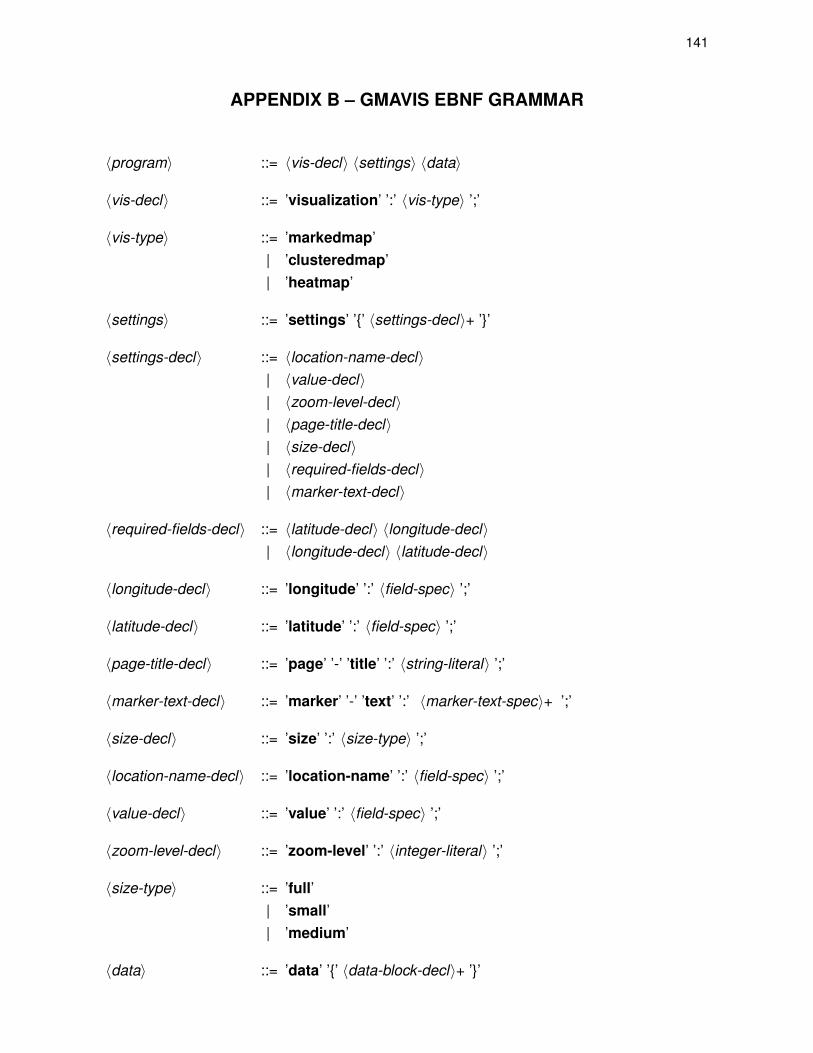
141

APPENDIX B – GMAVIS EBNF GRAMMAR

�program� ::= �vis-decl� �settings� �data�

�vis-decl� ::= ’visualization’ ’:’ �vis-type� ’;’

�vis-type� ::= ’markedmap’| ’clusteredmap’| ’heatmap’

�settings� ::= ’settings’ ’{’ �settings-decl�+ ’}’

�settings-decl� ::= �location-name-decl�| �value-decl�| �zoom-level-decl�| �page-title-decl�| �size-decl�| �required-fields-decl�| �marker-text-decl�

�required-fields-decl� ::= �latitude-decl� �longitude-decl�| �longitude-decl� �latitude-decl�

�longitude-decl� ::= ’longitude’ ’:’ �field-spec� ’;’

�latitude-decl� ::= ’latitude’ ’:’ �field-spec� ’;’

�page-title-decl� ::= ’page’ ’-’ ’title’ ’:’ �string-literal� ’;’

�marker-text-decl� ::= ’marker’ ’-’ ’text’ ’:’ �marker-text-spec�+ ’;’

�size-decl� ::= ’size’ ’:’ �size-type� ’;’

�location-name-decl� ::= ’location-name’ ’:’ �field-spec� ’;’

�value-decl� ::= ’value’ ’:’ �field-spec� ’;’

�zoom-level-decl� ::= ’zoom-level’ ’:’ �integer-literal� ’;’

�size-type� ::= ’full’| ’small’| ’medium’

�data� ::= ’data’ ’{’ �data-block-decl�+ ’}’

142

�filter-decl� ::= ’filter’ ’:’ �logical-expression� ’;’

�classification-block� ::= ’classification’ ’{’ �classification-decl�+ ’}’

�file-decl� ::= ’file’ ’:’ �string-literal� ’;’| ’h-file’ ’:’ �string-literal� ’;’

�structure-block� ::= ’structure’ ’{’ �structure-decl�+ ’}’

�data-block-decl� ::= �structure-block�| �classification-block�| �filter-decl�| �file-decl�+

�integer-literal� ::= ’integer literal’| ’-’ ’integer literal’

�field-spec� ::= ’field’ �integer-literal�

�expression� ::= �field-spec� ’is’ ’equal’ ’to’ �data-value�| �field-spec� ’is’ ’different’ ’than’ �data-value�| �field-spec� ’is’ ’greater’ ’than’ �data-value�| �field-spec� ’is’ ’less’ ’than’ �data-value�| �field-spec� ’is’ ’between’ �data-value� ’and’ �data-value�| �field-spec� ’contains’ �data-value�

�logical-expression� ::= expression| ’class’ ’(’ string-literal ’)’ ’:’ �logical-expression� ’;’| ’(’ �logical-expression� ’)’| �logical-expression� �connection-operator� �logical-expression�

�classification-decl� ::= �class-decl�

�string-literal� ::= ’string literal’

�format-decl� ::= ’format’ ’:’ �format-type� ’;’

�structure-decl� ::= �end-register-decl�| �date-format-decl�| �delimiter-decl�| �format-decl�

�marker-text-spec� ::= �field-spec�| �string-literal�

143

�connection-operator� ::= ’and’| ’or’

�date-format-decl� ::= ’date’ ’-’ ’format’ ’:’ �string-literal� ’;’

�char-literal� ::= ’character literal’

�float-literal� ::= ’float literal’| ’-’ ’float literal’

�data-value� ::= �date-value�| �integer-literal�| �string-literal�| �float-literal�| �char-literal�

�class-decl� ::= ’class’ ’:’ �logical-expression� ’;’| ’class’ ’(’ �string-literal� ’)’ ’:’ �logical-expression� ’;’

�format-type� ::= ’csv’

�delimiter-type� ::= ’tab’| ’newline’| �string-literal�

�date-value� ::= ’date’ �string-literal�

�delimiter-decl� ::= ’delimiter’ ’:’ �delimiter-type� ’;’

�end-register-type� ::= ’tab’| ’newline’| �string-literal�

�end-register-decl� ::= ’end’ ’-’ ’register’ ’:’ �end-register-type� ’;’