Embed Size (px)
Citation preview
/ J / / c...
PL-TR-95-2127 Environmental Research Papers, No. 1177
GLOSSARY FOR OVER-THE-HORIZON BACKSCATTER RADARS: Chapter 6, OTH Handbook
Editors: B. S. Dandekar J. Buchau
7 September 1995
APPROVED FOR PUBLIC RELEASE; DISTRIBUTION UNLIMITED.
19961127 010 DTIG QUALITY OGPBC3BD 8
PHILLIPS LABORATORY Directorate of Geophysics AIR FORCE MATERIEL COMMAND HANSCOM AIR FORCE BASE, MA 01731-3010

"This technical report has been reviewed and is approved for publication."
Tts
Maj Edward BerghjSrn, Chief Ionospheric Application Branch
WILLIAM K. VICKERY, Director Ionospheric Effects Division
This report has been reviewed by the ESC Public Affairs Office (PA) and is releasable to the National Technical Information Service (NTIS).
Qualified requestors may obtain additional copies from the Defense Technical Information Center (DTIC). All others should apply to the National Technical Information Service (NTIS).
If your address has changed, or if you wish to be removed from the mailing list, or if the addressee is no longer employed by your organization, please notify PL/TSI, 29 Randolph Road, Hanscom AFB, MA 01731-3010. This will assist us in maintaining a current mailing list.
Do not return copies of this report unless contractual obligations or notices on a specific document requires that it be returned.

REPORT DOCUMENTATION PAGE Form Approved
OMB No. 0704-0188
Public reporting burden for this collection of information is estimated to average j hour aathering and maintaining the data needed, and completing and reviewing the collection collection of information, including sugge«"""< ««' rMiudna thk burden, to wasninaton Davis Highway. Suite 1204. Arlington, VA
per response, including the time for rev.ewmg instructions, searching existing datasources , of information. Send comments regarding this burden estimate or anyother aspen of this Headauarters Services. Directorate for information Operations and Reports, 1215 Jefferson
cSn^formatioAludi^sug^
1. AGENCY USE ONLY (Leave blank) 2. REPORT DATE 3. REPORT TYPE AND DATES COVERED
SmWifir. Tntmm
4. TITLE AND SUBTITLE Glossary for Over-the-Horizon iBackscatter Radars: Chapter 6, OTH Handbook
6. AUTHOR(S)
B. S. Dandekar and J.Buchau, Editors
7. PERFORMING ORGANIZATION NAME(S) AND ADDRESS(ES)
Phillips Laboratory (GPIA) 29 Randolph Road Hancsom AFB, MA 01731-3010
9. SPONSORING/MONITORING AGENCY NAME{S) AND ADDRESS(ES)
5. FUNDING NUMBERS
PE 62101F Proj 4643 TAGH WU 01
PERFORMING ORGANIZATION REPORT NUMBER
PL-TR-95-2127 ERP,no. 1177
10. SPONSORING/MONITORING AGENCY REPORT NUMBER
11. SUPPLEMENTARY NOTES
This report was completed to assist the operators managing the OTH radars deployed by the US Air Force.
12a. DISTRIBUTION/AVAILABILITY STATEMENT
Approved for Public release; Distribution Unlimited
12b. DISTRIBUTION CODE
13. ABSTRACT (Maximum 200 words)
This report explains frequently used scientific (geophysical) and engineering terms that all kinds of operators managmg/running the Over-the-Horizon Backscatter Radar Systems need to understand. As the ionosphere is an integral part of the radar operation the operators must be familiar with geophysical phenomena that affect the ionosphere, as well as with the engineering terminology of the functioning of the radar system.
14. SUBJECT TERMS
OTH radars, Ionosphere, Magnetic activity, Auroral oval.
17. SECURITY CLASSIFICATION OF REPORT
Unclassified NSN 7540-01-280-5500
18. SECURITY CLASSIFICATION OF THIS PAGE
7T«/.1accifigH
19. SECURITY CLASSIFICATION OF ABSTRACT
TTt^laooifiAH
15. NUMBER OF PAGES
86 16. PRICE CODE
20. LIMITATION OF ABSTRACT
-SAEL
DTIC QUALITY INSPECTED 3 Standard Form 298 (Rev. 2-89) Prescribed by ANSI Std. Z39-18 298-102

Contents
1 1. INTRODUCTION
2. GLOSSARY FOR THE OTH RADAR OPERATION 2
3. OVER-THE-HORIZON BACKSCATTER (OTH) RADAR SYSTEM CONCEPTS 3
4. TEAM ACTION AT THE OTH OPERATIONS CENTER 7
5. DEFINITIONS 8
Absorption of Radio Wave Energy 8
AN/FPS 118 8
Appleton or Equatorial Anomaly 10
Aurora 10
Auroral Absorption 10
Auroral Clutter 12
Auroral Oval *2
Auroral Substorm 12
Auroral Zone "
Backscatter ^
Backscatter Sounder 15
Barrier 18
Blind Speed Unmasking (BSUM) 18
CCIR (International Radio Consultive Committee) Noise Levels 18
Clutter, Ground 19
Clutter, Ionospheric/Auroral 19
Clutter-to-Noise Ratio (CNR) 20
Coherent Integration Time (CIT) 20
Coherent Radiation 20
Coherent System 21
in

Coning 21
Coordinate Registration ^
Coronal Hole ^
Coronal Mass Ejection ^
Critical Frequency ■"
D Layer (D-Region) ^
dB, Decibel 24
Detection/Tracking Algorithm 25
Digital Ionospheric Sounding System (DISS) 25
Dipole field 26
Disappearing Solar Filaments 26
Doppler, Doppler Shift 26
Doppler Resolution 28
E Layer (E-Region) 28
E Layer Masking 29
East Coast Radar System (ECRS) 29
Electron Density Gradient 29
Elevation Angle 29
Equatorial Plasma Depletion 29
Equatorial Spread Clutter 31
Experimental Radar System (ERS) 3 *
Extended Azimuth and Range (EAR) 3 *
F Layer (F Region) 32
Faraday Rotation 32
Field Aligned Scatter (Orthogonal Scatter) 33
FM/CW Modulation 33
Geomagnetic Disturbance 34
Geomagnetic Field 34
Geomagnetic Storm 34
IV

Great Circle Propagation 34
Ground Clutter 35
High Frequency (HF) Electromagnetic (Radio) Waves 35
Incidence: Vertical and Oblique 35
Ionizing Solar Electromagnetic Radiation 36
Ionogram
Ionosonde
Ionosphere
Line of Sight
37
Ionospheric Irregularities 38
Ionospheric Seasons
Ionospheric Sunrise/Sunset
Libration Point (Lagrangian Point Lt) 4°
38
39
40
Linear Antenna (Coning) Theory 4°
Lowest Usable Frequency (LUF) 41
M-Factor
Magnetic Activity Indices
Magnetic Coordinate System
Magnetic Equator
Magnetic Field
Magnetic Time
Magnetometer
Magnetosphere
Maximum Observed Frequency (MOF) ^
Maximum Usable Frequency (MUF) 47
47 Meteors
Midpoint Ionosphere
Mode(s)
Model, Ionospheric
41
42
44
44
44
46
46
46
48
48
48

52
52
53
Morphology of the Ionosphere 49
Noise 49
Nuclear Effects 50
Off Great Circle Propagation 50
Operational Radar System (ORS) 50
Over the Horizon (OTH) Backscatter Radars 51
Plasma
Plasma Frequency
Polar Cap
Polar Cap Absorption (PCA) 53
Probability of Correlation Pc 53
Probability Of Track Establishment (Detection) -PD 54
Propagation Modes ^
Radar Cross Section ^
Radar Cross Section of a Fully Developed Sea 56
Radar Cross Section of Ice 56
Radio Wave Polarization 56
Range Folding 57
Range (Clutter) Related Noise 57
en Range Resolution
Reflection, Ionospheric 58
Refraction, Ionospheric 58
Relative Ionospheric Opacity Meter (Riometer) 59
Scatter
Signal to Noise (S/N) Ratio
Skip Zone
Solar Active Region 61
Solar Activity (Sunspot) Cycle 61
Solar Cycle 63
59
59
59
VI

Solar Flare 63
Solar Maximum "4
Solar Minimum ^4
Solar Rotation M
Solar Wind M
Spectrum Analysis "5
Specular Scatter ^6
Sporadic E &
Spread F 67
Storm Sudden Commencement 67
Sudden Ionospheric Disturbance (SID) 67
Sunspots 68
Sunspot Number (SSN) 68
Terminator 68
Trapped Mode 69
Traveling Ionospheric Disturbance (TID) 69
Universal Time (UT) 70
Vertical Incidence (VI) 70
Virtual Height 70
Waveform Bandwidth (WB) 71
Waveform Repetition Frequency (WRF) 71
Zenith Angle 71
BIBLIOGRAPHY 73
VI1

Illustrations
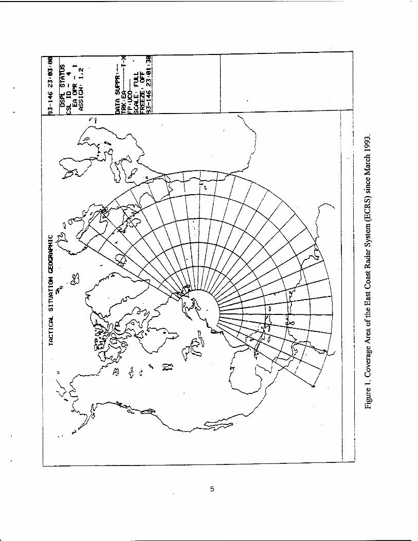
1. Coverage Area of the East Coast Radar System (ECRS) since March 1993. 5
2. Radar Ray Paths and Doppler Signatures of Clutter, Target, and Noise
for the Surveillance Barrier. 6
3. Ionospheric Layers and the Electron Density Profiles for Day and Night Conditions. 9
4. Latitudinal Variation of Electron Density Across the (Appleton or) Equatorial
Anomaly at Various Altitudes Above h,,,« (F- layer maximum) From Topside
Ionograms (Eccles and King 1969, Reprinted With Permission From IEEE 1969). 11
5. Location of Experimental Radar Sector (ERS) With Respect to the Auroral Oval
at 00, 06, 12 and 18 UT. 13
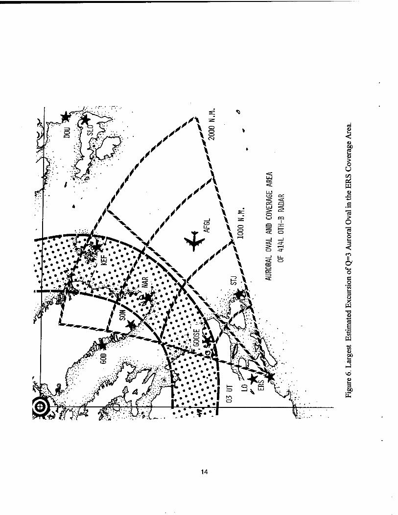
6. Largest Estimated Excursion of Q=3 Auroral Oval in the ERS Coverage Area. 14
7. Morphology of the Ionosphere Showing Locations of Appleton Anomaly, High
Latitude F Layer Trough, Auroral and Polar Cap Regions; Also Shows ECRS
and WCRS Coverage Areas. 16
8. Backscatter Ionogram From a Backscatter Sounder. 17
9. The Magnetic Field of Earth, a) Dipole Model, b) More Realistic Field Transformed
Under the Influence of the Solar Wind. 27
10. Effect of E Layer Masking on the Target Signal. 30
11. Comparison of Sunspot Cycle With Magnetically Disturbed Days (SKp >25). 43
12. North Polar Map Plotted in Corrected Geomagnetic Coordinates. 45
13. Propagation Modes in the Ionosphere. 55
14. Location of the Skip Zone and the Barrier. 60
15. Sunspot Cycles for the Period 1816 to 1989 62
Vlll
OTH GLOSSARY CONTRIBUTORS
W. Abel** and others MITRE
Su. Basu Emmanuel College
K. Bibl University of Massachusetts, Lowell, MA
C. Bowser Martin Marietta
J. Buchau* Compiler and Editor, Phillips Laboratory
E. Cliver Phillips Laboratory
R. I. Coman**, Capt Acquisition Meteorology (WE), Electronics
System Center
B. S. Dandekar Compiler and Editor, Phillips Laboratory
J. R. Jasperse Phillips Laboratory
M. M. Klein** Phillips Laboratory
J. G. Moore** University of Massachusetts, Lowell, MA
G. S. Sales University of Massachusetts, Lowell, MA
K. Toman** Rome Laboratory
E. J. Weber Phillips Laboratory
B. Weijers Rome Laboratory
J. A. Whalen Phillips Laboratory
"Deceased
**Retired
IX
Acknowledgements
The authors thank Major Edward Berghom, Major Vincent Azzarelli and Mr. John Heckscher
for their valuable suggestions.
XI

Glossary for Over-the-Horizon Backscatter Radars
Chapter 6, OTH Handbook
1. INTRODUCTION
This report provides a quick reference, and, for improved understanding, a list of
terminologies and a short description of the essential terms usually encountered by the radar
operators. We have made an effort to include most of the terms usually encountered in the OTH
operation. However, users of the glossary may need 1) to have additional terminologies included
and 2) get more clarification of some terms already in the glossary. Therefore we would
encourage feedback and comments. Please feel free to contact:
Dr. B. S. Dandekar Phillips Laboratory /GPIA 29 Randolph Road Hanscom AFB, MA 01731-3010.
With the deployment of the OTH radars, a need for an OTH Handbook that would provide a
basic understanding of the OTH operation, the general layout of the radar structure, and the basic
geophysics background was realized by the community. With the help of the OTH community,
Jürgen Buchau took the lead and accepted the responsibility for producing the OTH Handbook.
The planned handbook has six chapters. These are 1) Introduction, 2) OTH Radar System:
System Summary, 3) Physics of the Ionosphere for the OTH Operation, 4) High Frequency (HF)
Radiowave Propagation, 5) The OTH Radar Operation and 6) Glossary for OTH Radars.
Chapters 2 and 4 have been published by Dr. Gary Sales as technical reports (see reference). This
glossary is included as Chapter 6 of the handbook. The remaining chapters will be published as
separate reports.
Received for publication 6 September 1995.

2. GLOSSARY FOR THE OTH RADAR OPERATION
Radar operation involves Environmental Assessment (E/A) operators, Correlation and
Identification (C/I) operators, Detection and Tracking (D/T) operators, and Radar Control and
Monitor (RC&M) operators. The E/A operators help the radar managers with the important task
of selection of the operating frequency of the radar, which depends upon the selected sector, time
of the day, and the state of the ionosphere, which is an integral part of the OTH radar system; the
system simply cannot work without the cooperation of the ionosphere over the coverage area.
The EA operator needs some background on the subject of the ionosphere such as its production
and depletion, its spatial and temporal behavior, and the way it is affected by phenomena such as
solar flares, solar winds, magnetic storms, polar cap absorption events, aurora, etc. The other
operators (D/T, C/I, RC&M) need an engineering background for the operation of the radar, in
which terminology such as coherent integration time, signal to noise ratio, wave repetition
frequency etc is often used. We hope this glossary satisfies these needs of the operators.
3. OVER-THE-HORIZON BACKSCATTER (OTH) RADAR SYSTEM CONCEPT
An OTH radar system detects and tracks aircraft far beyond the line-of sight horizon of
conventional radars out to distances of up to 1800 nautical miles. (The range was extended to
3000 nmi initially in the south-looking sector-3 of the East Coast Radar System (ECRS), and
since March 1993, in all three sectors.) Figure 1 shows the present coverage of the East Coast
Radar System. The figure shows 24 beams and each semicircle indicates a range at an interval of
500 nmi. The beams are numbered starting from north. Each group of 8 beams forms a sector.
The sectors also are numbered 1, 2, 3, starting from north. Each beam has a width of 7.5° in
azimuth. Thus each sector covers an azimuth range of 60°. Note that the beams were rotated 15°
from the initial configuration and the range was increased from 2000 nmi to 3000 nmi. This
change provides a coverage of the South American region for drug interdiction. The barrier is
established starting at a range of typically 1000 to 1200 nmi and extending outward approximately
500 nmi by reflecting radio waves in the HF band (3 to 30 MHz) from the ionosphere (Figure 2).
Part of the HF energy reaching the ground in the barrier is backscattered to the radar by the rough
ocean and land surface. It is called clutter or ground clutter. The clutter normally has the exact
frequency of the transmitted signal (zero Doppler). A moving aircraft scatters back energy at a
frequency shifted (Doppler shifted) by the motion of the aircraft.
The spectrum analysis of the total backscattered signal permits the separation of the
returns into clutter at zero Doppler and target at a Doppler frequency proportional to its
approaching (positive Doppler) or receding (negative Doppler) radial velocity (for convenience,
positive and negative Doppler are reversed on the screen display).
Measuring the total travel time of the signal from the transmitter to the target and back to
the receiver yields the radar range of the target. Using the ionospheric reflection height of the
signal, the "ground range" of the target can be determined. The ground range and the "ground
azimuth" derived from the direction of the antenna beam in which the target is observed yield the
geographic coordinates of the target location. Observing the target for extended periods permits
the tracking of its flight path.
Radio energy from various sources received in the Doppler interval away from the ground
clutter is noise. It is against this noise background that the target must be detected . This noise

background originates from natural (atmospheric) and manmade emissions and under certain
conditions from backscatter of the radar's own signal from ionospheric and auroral
irregularities. When the noise from ionospheric and auroral scatter exceeds the target signal
level at the appropriate (the target's) Doppler, detection of the target will be impossible. This
represents the main area of radar performance degradation observed during the test period of the
Experimental Radar System (ERS).
(For a partial listing of test and operational OTH radars and programs, see OTH Radars).
c3
CO
o
tä 5-.
CO i~ 03
CO O u
-4-» 1/1 «3 w u
•♦■J
<4-C
O CO
(50 2 > o u
w 3 00 s

'£ cd
m u u c
_cd
'53
3
(Si
*-> s-
CO
c cd
0)
£P cd H i-T 0)
■4-»
3 Ö (4-1 o
en
CO C SP
c/3 t-i
"a« o Q *o c
cd VI
Id HH
u. ed
"O cd ej <N
<u u 3 00 E

4. TEAM ACTION AT THE OTH OPERATIONS CENTER
Here is a brief description of how operators and supervisors work together to meet
mission objectives. The Detection and Tracking (D/T) operators monitor the automated D/T
processes and use the displays and controls to maintain the targets (incoming aircraft) processed
from the radar returns. Following the recognition of a target (aircraft) by the D/T operators, this
information is passed to the Correlation and Identification (C/I) operators, who monitor the C/I
process and assign correlated track/flight path pairs based on system generated automatic
recommendations. The most important function is to identify the targets, track their paths to
determine their nature (friend /enemy), and resolve the uncertain tracks into false signals or
unidentified targets, which are then transmitted up the chain of command for further action. The
radar is under the direct control of the Radar Control and Monitor (RC&M) operator, who
selects parameter sets prescribed by differing mission objectives. Frequency selection is based on
the range requirements associated with the mission. These are generally determined by automated
processes that include the Environmental Assessment (EA) function. An important system
interface for the Environmental Assessment is the development of the Coordinate Registration
(CR) tables, which the system uses to convert radar slant range to ground range. As can be seen
in Figure 2, the distance between the radar and the target along the earth's surface is the ground
range, whereas the radar measures the distance along the raypath (the slant range) as a time delay
between the transmitted and received signals for the correlation process. The Senior Director
(SD) is responsible for the orchestration of the system according to tasking from higher authority,
and is responsible for reporting the radar availability and performance to higher headquarters.
The Station Director is responsible for the management of all the system resources.

5. DEFINITIONS
A
ABSORPTION OF RADIO WAVE ENERGY (Buchau)
Radio waves propagating through the ionosphere cause the ambient free electrons to oscillate
with the frequency of the radio waves. When these oscillating electrons collide with molecules or
atoms of the neutral atmosphere, they lose their energy, thereby weakening the radio wave. This
process is called absorption. It is especially effective at lower ionospheric altitudes, especially in the
D-region (see Figure 3 for ionospheric layers), where due to the high neutral density, the frequency
of collisions is very high. Since the D-region is predominantly produced by solar UV and X-Ray
emissions, radio wave absorption is mainly a daytime phenomenon. Strong enhancements of the D-
region ionization due to solar flares, auroral substorms, or energetic solar protons (see under PCA)
result in strong enhancements of radio wave absorption. At night, with the D-region ionization
source turned off, the strong radio wave absorption originating in the D region vanishes. This makes
night time HF communications over long distances possible even at low transmit power levels.
Absorption 'L' is strongly frequency dependent, following an inverse square law L ~ 1/f2
which means that doubling the operational frequency will result in a decrease of the level of
absorption by a factor of 4. A 10 percent increase in frequency results in an 18 percent reduction in
absorption. It is therefore important for power-limited systems to operate at as high a frequency as
possible (MUF, MOF).
AN/FPS118 (Buchau/Dandekar)
AN/FPS 118, is the Air Force designation of the OTH-Backscatter System, built by the
General Electric Corporation to government specifications. It is deployed in Maine with the
operations center at Bangor, Maine, to cover the Atlantic off the East Coast (East Coast Radar
System or ECRS) and in California and Oregon, with the operations center at Mountain Home,
Idaho, to cover the Pacific off the West Coast (West Coast Radar System or WCRS). The former
is currently operated by the Radar Squadron (RADS) DET1/NEADS (North East Air Defense
Sector) of the Air Combat Command (ACC).

THE IONOSPHERE PROFILE
LU Q
b <
10 icr ioJ 10" 10" \cr
ELECTRON DENSITY (ELECTRONS PER CM3)
Figure 3. Ionospheric Layers and the Electron Density Profiles for Day and Night Conditions.
9

APPLETON OR EQUATORIAL ANOMALY (Weber)
These are two bands of increased F-region electron density centered at - ±15° magnetic
latitude and'extending in local time from noon to after midnight with maximum development in the
afternoon. They may change from day to day in their maximum electron density and exact location
under the influence of varying geophysical conditions. The region is produced by the upward motion
of ionospheric plasma (across magnetic field lines) at the equator and downward drift of this
plasma (along field lines) to form a region of increased density away from the equator. Figure 4
shows a typical observed distribution of electron density with latitude, at several altitudes determined
from topside ionograms. Note that there are two maxima in electron density with a minimum at the
magnetic equator. This feature is called the Appleton or equatorial anomaly. Because of the increased
density, the region is characterized by increased airglow and by large horizontal electron density
gradients. The gradients, and the irregularities developing in the Appleton Anomaly in the post
sunset-to midnight period (Equatorial Plasma Depletion), can produce ionospheric clutter on
south-looking radar beams. Since every great-circle path crosses the equator, ionospheric clutter
originating from equatorial regions may range fold into the barrier if propagation conditions and
irregularity intensities are appropriate.
AURORA (Whalen)
The aurora is light produced when electrons and protons from space (the magnetosphere)
strike the earth's upper atmosphere. The ionization that is also produced in this process can affect
OTH performance in a number of ways (auroral absorption, auroral E layer, E layer masking,
auroral clutter). Ionization resulting from the precipitation of auroral particles is often called auroral
ionization, in contrast to solar produced ionization (see Ionizing Solar Electromagnetic Radiation).
AURORALABSORPTION (Whalen)
The attenuation of radio wave energy as it passes through ionization produced by auroral
particle precipitation is called auroral absorption. This ionization usually occurs at D region altitudes
(50-90 km) and is produced by auroral electrons of greater than 40 keV energy. A band of
absorption is located typically at the low latitude edge of the auroral oval at midnight but can extend
10

£ o
i- < er Z UJ o z o o
o or o tu _j UJ
0° +10° +20° +30°
GEOGRAPHIC LATITUDE(degrees)
Figure 4. Latitudinal Variation of Electron Density Across the (Appleton or) Equatorial Anomaly at Various Altitudes Above ^ (F- layer maximum) From Topside Ionograms (Eccles and King 1969, Reprinted With Permission From IEEE 1969).
11

to all local times at nearly constant magnetic latitude. During disturbances (substorms,
geomagnetic storms) both the size of the absorption band and the level of ionization can increase
greatly. (See also under absorption).
AURORAL CLUTTER See Clutter, Ionospheric/Auroral
AURORAL OVAL (Whalen)
In a band encircling the magnetic pole, the aurora and auroral ionization occur. This oval
is farthest north (poleward) and narrowest in the daytime; farthest south (equatorward) and widest
at night. (An identical band encircles the geomagnetic south pole). Figure 5 shows the daily
variation of the oval (the band between the solid circular lines) at four different Universal Times (UT).
This daily variation causes the oval to intrude into the East Coast Radar System (ECRS) coverage
area (shown shaded) more at local night (near 00 UT) than in the daytime (near 12 UT). For the
West Coast Radar System (WCRS) oval, intrusion near 12 UT skirts the northernmost sector (3-8).
However, propagation and ionospheric clutter effects associated with the F Layer Trough, which
is just equatorward of the auroral oval, increase the effective diameter of oval related disturbances.
Figure 6 shows a segment of the ECRS and the auroral oval for 04 UT (midnight in the center of the
coverage). This represents the deepest penetration of the oval into the coverage for a slightly
enhanced magnetic activity condition (Q=3), (see magnetic activity index, substorms, geomagnetic
storms), when the oval widens and moves to the south (equatorward). Ionization is also increased
during such disturbances so that the impact on OTH is two-fold: more intense ionospheric effects,
which are more widespread within the coverage area. For additional details on the ionosphere in the
vicinity of the auroral oval see under Morphology, Ionosphere.
AURORAL SUBSTORM (Whalen)
This is a relatively short term disturbance (typically 2 hours) during which the aurora and
auroral ionization increase and the auroral oval widens and moves equatorward. The rate of
occurrence of auroral substorms is about 2 to 4 per day, with substantial enhancements in occurrence
and intensity during large geomagnetic storms.
12

O cT O
o O u.
JS
u OH
Pi
CO pi
O <u V3 i-i «J
"O
I ■s s
"C o.
«4-1 o e o '3 o o
3 SO S
13
OH.
CD
a:
<c i
CD
a; O a:
a en
PQ I
u
O U
J2
CO > o o u.
II a <*- o c o
3
PE] ■4-J vx a> öO tö
2 3 60 S
14

AURORAL ZONE (Whalen)
It is a region in which the aurora is most likely to occur near local midnight. It is a band
encircling the magnetic pole with its southern boundary near 65° corrected geomagnetic latitude.
(See Figure 7, Morphology of the Ionosphere).
B
BACKSCATTER (Sales)
A target, or any physical object, in the path of the radar beam scatters a portion of the radar's
energy back towards the radar. This returned signal is called backscatter. Backscatter occurs
whenever either a distributed target, that is, a target that tends to fill the radar beam, or a point target,
one that occupies a small fraction of the radar beam, is present. Land or sea surfaces are typical
distributed targets. Another example is a large volume of intense ionospheric irregularities. An
aircraft or a ship, on the other hand, is considered a point target.
The amplitude of the backscattered signal depends on the surface or volume characteristics
of the target as well as the cross-sectional area it presents to the radar beam. For a typical OTH
radar, the sea/land surface in the beam of the radar has an area of 1013 m2 and taking into account the
efficiency of the backscatter process, these surfaces have an effective area of 10u m2, compared to
a medium or large aircraft with an area of 102 to 103 m2.
BACKSCATTER SOUNDER (Buchau)
This system measures and displays backscattered energy as a function of frequency and range.
By sweeping in frequency (usually 2-30 MHz), the backscatter sounder provides a measure of the
skip distance as a function of frequency. Figure 8 shows a backscatter ionogram from a backscatter
sounder. The edge of the dark trace running from 210 nmi for 2.5 MHz to 1070 nmi for 30 MHz is
the skip distance for the respective frequency. Therefore, a backscatter sounder assigned to each
azimuth sector provides a convenient means for determining the maximum usable frequency (MUF)
over a wide geographical area. Backscatter sounder based real-time frequency management is
therefore available at all OTH radars, often as an integral part of the environmental assessment (EA)
and Radar Control (RC) functions of the radars.
15

J3 "o Pi
C cd
"e3 u O u
.C 00 3 O u. H w-
t> 3 +■* "J es .J 60
s "3 S o
c o
"3. <■
O co
.2 5 es ai O «■ O
HJ
60 c I o
CO
p
Q. en O c o
3» u u > o U CO
U
C es
0)
*-> CM o to;
CO OS u w CO
o
^'o O 00
&^ O co
s §
s * 3 a, 60 cS
16

CO
05 CO
V o c CO *-* en
a. CO
co
60 •a 00 c
^3 cd
as
of s c
'5b
o
I-.' 0)
•s 3 o
00 s- <u
■+->
to o CO
o CO
« CO
O to
i_ C ÖD ü O 3 c cr o g
Ü .S
«s o w o od JS ü .2 3 O 00 C E <3
17

BARRIER (Buchau)
A barrier is a continuous band of OTH surveillance coverage of sufficient width to permit the
OTH radar to detect and also track aircraft traversing this band. Typically, ECRS and WCRS
radars position the barrier start at 1000 nmi. The OTH radar, through proper frequency management,
attempts to illuminate this barrier continuously with radio energy refracted from the ionosphere to
detect and track all aircraft crossing it. While the desired barrier width is 500 nmi, a distance which
a typical jet aircraft traverses in about an hour, and the maximum instantaneous range over which the
radar can collect track data, the ionosphere does not always illuminate a 500 nmi wide band. Narrow
barriers are typical for sunrise transition and are due to ionospheric tilts and lowered ionospheric
electron density in the reflection region.
BLIND SPEED UNMASKING (BSUM) (Abel)
The unambiguous Doppler range available in the spectrum analysis is given by the Nyquist
theorem as 1/2 the sampling rate. Higher Doppler frequencies are aliased or folded into the
unambiguous Doppler window, that is, they appear in a well defined but wrong location in the
spectrum. In the OTH Doppler processing, they actually appear in adjacent range bins. If the target
velocity is so high that the Doppler shift equals the WRF (waveform repetition frequency), which
is also the sampling rate, that is, if Af=2vf7C0 =WRF, the target return is Doppler shifted into the
next ground clutter line and therefore is undetectable. The target is flying at 'blind' speed. Changing
the WRF by more than the width of the ground clutter line (in Hz) 'unmasks' the target. The OTH
radar has a Blind Speed Unmasking (BSUM) option, which for each primary WRF automatically
selects a secondary one, which will unmask aircraft flying at the blind speed.
C
CCm NOISE LEVELS (Sales)
CCIR is the abbreviation of an organization entitled the International Radio Consultive
Committee. They have generated a report (No. 322) dated 1963, entitled World Distribution and
Characteristics of Atmospheric Radio Noise which has been updated by A. D. Spaulding and J. S.
Washburn (NTIA report 85-173 April 1985). This report summarizes the results of noise
18

measurements over the frequency range 10 kHz to 100 MHz from 16 stations spread over most of
the globe. The report establishes median values and other statistical characteristics of the noise for
all points on the earth as a function of time and season. These data represent a standard against
which any system can be assessed in regard to its expected performance in the noise environment.
CLUTTER, GROUND (Buchau)
Radio energy refracted back to earth from the ionosphere (obliquely) is primarily reflected
from the ground in the forward direction away from the radar. However, the inherent roughness of
the land or sea surfaces causes a small part of the incident energy to be scattered in all directions
including back towards the radar. The part of the scattered energy that retraces the original path back
to the transmitter, is called ground backscatter or ground clutter. The ground clutter is
backscattered with little or no Doppler shift from the ocean or land surface within the radar beam.
The clutter amplitude is a function of the antenna beam-width, the pulse width, the transmitted power,
and the scatter efficiency of the land/ sea surface. Besides these parameters, the amplitude of the
ground clutter is also controlled by conditions in the ionosphere (absorption, irregularities,
gradients). The ground clutter received by the radar is a measure of the amount of energy deposited
in the coverage region and therefore also on any target(s) that may be present. The probability of
detection (PD) for a given aircraft size can be determined from a comparison of ground clutter and
noise levels (clutter-to-noise-ratio). Aircraft moving relative to the radar have their returns Doppler
shifted, a fact that is used to separate target returns from the much stronger ground clutter which has
little Doppler shift (see spectrum analysis).
CLUTTER, IONOSPHERIC/ AURORAL (Sales)
Randomly moving irregularities in the ionosphere scatter a portion of the radar's own signal
back to the radar. The motion of these irregularities spreads the backscattered radar signal over a
range of velocities. When these irregularities occur at the range of the targets, and the velocities of
the targets, the scattered signals will tend to obscure the detection of the aircraft.
19

CLUTTER-TO-NOISE RATIO (CNR) (Buchau & Sales)
Measuring the ground clutter amplitude of the radar signal provides a measure of the energy
deposited in the barrier and available for the illumination of targets. For a given radar system and
specified system operating parameters, the ratio of the power in the ground clutter to the power
scattered back from an aircraft is, in first approximation, a constant. Ionospheric losses (absorption,
defocusing, scattering due to irregularities) in general affect clutter and signal (target) amplitudes
the same way. Therefore, the ratio of the clutter to the noise power can be used to infer the target-to-
noise (signal-to-noise) ratio as a measure of target detectability. The CNR has been calibrated in
terms of probability of detection PD and has been used extensively to infer system performance in
areas and during times of low air traffic density.
COHERENT INTEGRATION TIME (CIT) (Abel)
Each signal waveform reflected from a target contains a target echo plus noise. These
waveforms are summed up(integrated) by matching the starting phase (of each waveform) to increase
the signal/noise ratio. The signal enhancement is proportional to N2 (in power or N in amplitude),
with N being the number of samples summed. Noise is random and is enhanced proportional to N
(in power or VN in amplitude). If the target echoes are in phase, that is, arrive at the radar at the
same time relative to the start of each waveform time period, the improvement in signal/noise is
proportional to N (in power, or VN in amplitude). The time interval during which waveforms are
summed up by matching the starting phase, is called the coherent integration time. This time is
limited by the characteristics of the propagation path. Only time durations over which the path
characteristics stay stable, resulting in a coherent signal, are suitable for coherent integration.
COHERENT RADIATION (Abel)
This is radiation for which the frequency of the signal with respect to a frequency standard
is stable. With respect to a radar, coherent implies that the signal phase of the transmitted waveform,
either pulse or FM/CW, is constant with respect to the start of the waveform. This is achieved by
deriving all frequencies used to generate the transmit waveform from a common source (stable
oscillator). Likewise a coherent receiver is a receiver, where all frequencies used in the receiver chain
20

are derived from a single, stable frequency source. The OTH radars are coherent systems. This
ensures that radar signals reflected at a stationary reflector arrive at the receiver with exactly the
same phase in relation to, for example, the start of the FM/CW waveform (assuming a stable
ionospheric reflector). Sampling of the received signal in fixed relation (phase) to the waveform start
will result in sampling of the signal at a constant phase angle, thereby allowing coherent integration,
that is, the coherent signal samples are added linearly with each sample, the resulting summed
amplitude is proportional to the number N of the samples. For a moving reflector (target), the phase
of the received signal changes in proportion to the change of the phase path, that is, in proportion to
the reflector velocity relative to the radar. Coherent sampling allows determination of this phase shift
and thereby the Doppler shift of the target. This fact is used by the OTH radars to separate the non
Doppler shifted ground clutter from the moving target return.
COHERENT SYSTEM (Buchau/Abel)
A coherent radar system requires that all frequencies used in both the transmitter and receiver
components are derived, by multiplication and division, from the same standard frequency source
(often 1 or 5 MHz) or from two independent frequency sources that are kept synchronized, by
comparison to a third stable frequency source such as LORAN-C transmissions, so that if they were
brought together there would be no phase difference between them. This coherence allows the
repeated transmitted waveforms to always begin with the same phase for as long as the radar dwells
in one beam position. Even the digital sampling pulses, at the output of the receiver, are derived from
the same standard frequency source so that the digital samples of the received signal maintain a fixed
phase relationship from waveform repetition to waveform repetition. This allows the target signal
to be summed over a period of time called the dwell time or the coherent integration time (CIT),
using samples from successive waveforms with little change in either the amplitude or phase of the
signal, assuming the ionospheric path is relatively stable. Superimposed on the target signal is a
random noise signal, either originating internally to the receiver, or externally from atmospherics or
of man made origin from industrial machinery. While the phase of the target signal is relatively
constant during the dwell time (commonly a CIT of 1-2 s is used, resulting in a sum of 40 to 80
waveforms when WRF = 40 Hz) the phase of the noise signal changes randomly, and the sum tends
21

to increase more slowly for the noise than for the target component of the signal, resulting in an
overall target (signal) to noise ratio improvement. This improvement is proportional to N (for signal
to noise power ratio) where N is the number of waveforms summed (integrated) in one dwell period.
Another approach to this coherent integration process is particularly useful when the target is moving
relative to the radar (either approaching or receding). Then, spectrum analysis of the combined
digitally sampled target and noise signals accomplishes the same coherent integration for the target
signal and noise but makes it possible to separate different targets moving at different velocities
(different Doppler frequencies) from each other and from the very much stronger ground clutter
signal, which has zero Doppler shift.
CONING see LINEAR ANTENNA THEORY
COORDINATE REGISTRATION (CR) (Weijers)
The coordinate registration (CR) process develops a virtual height data base, maintains a real-
time model and establishes coordinate conversion tables. These tables provide information necessary
for converting the radar slant range and the apparent angle of arrival into ground range and a true
azimuth to determine the ground coordinates of the targets detected. The maintenance and update
of the CR process is mainly accomplished from data stored in the model and the vertical incidence
sounder data base. Additional techniques available use terrain features observed in backscatter
ionograms, and flight plan updates from aircraft with precision navigation equipment. The update
process can be either manual or automatic.
CORONAL HOLE (Cliver)
Extreme Ultra-Violet (EUV) and soft X-ray images obtained by instruments aboard rockets
and spacecraft in the early 1970s showed cool dark regions in an otherwise bright corona (the outer
atmosphere of the sun). For this reason they were named coronal holes. These holes mark regions
of open magnetic field lines along which solar wind particles can easily escape the sun. Coronal holes
have been identified as the source of high speed streams in the solar wind that give rise to recurrent
22

(every 27 days) geomagnetic storms. Coronal holes may appear either at the poles of the sun or near
the equator. The holes lying closest to the equator, which rotate at the 27 day solar rate (see solar
rotation), are the more geophysically significant.
CORONAL MASS EJECTION (Cliver)
A coronal mass ejection (CME) is a cloud of magnetized plasma that moves outward from
the sun with a speed that may range from 50 km/s to 2000 km/s. CMEs having speeds > 500 km/s
are often accompanied by coronal and interplanetary shock waves. CMEs may be associated with
either eruptive solar flares or disappearing solar filaments. As with flares and sunspots, the
occurrence rate of CMEs varies with the sunspot cycle. CMEs represent the causative link between
the sun and the magnetosphere in the production of non-recurrent geomagnetic storms.
CRITICAL FREQUENCY (Buchau / Dandekar)
The critical frequency is a limiting frequency below which a radio wave is reflected by, and
above which the wave penetrates and passes through an ionized medium ( for our application, an
ionospheric layer) at vertical incidence. The critical frequency (f0) is a measure of the maximum
electron density of a layer, f0 = 8.98 x 10"3 -/Ne with f0 in MHz and Ne in el cm"3. The critical
frequency of a layer allows an operator to estimate the highest frequency that can be propagated via
that layer. As a rule of thumb, to a distance of 1100 nmi (-2000 km), the typical OTH barrier start
distance, the F-Iayer allows propagation with frequencies up to f^ = 2.3 x foF2, where f0F2 is the
critical frequency of the F (F;) layer. For E-layer reflection, the multiplier to the same distance is 5.
D
D LAYER (D-REGION) (Jasperse)
This portion of the ionosphere extends in altitude from about 50 to 90 km (27 to 49 nmi)
where solar radiation ionizes the atmospheric particles to produce a layer that is the principal agent
of the absorption of radio wave energy. The D region is responsible for most of the absorption
23

of radio waves in the frequency range from 1 to 100 MHz. During solar flares, the D region may
be lowered by as much as 15 km by an enhanced flux of X-rays. Energetic particle precipitation at
auroral and polar cap latitudes enhances the D region (see Figure 3 for ionospheric layers), resulting
in auroral absorption and polar cap absorption (PCA) events.
dB, DECIBEL (Buchau)
The decibel is a unit for the comparison of power levels. It represents the ratio of two power
levels and is defined as
NdB = 10 log P^ or 10 log P«/Prcf
P0 = output as signal power
Pj = input power
Pref = reference (zero) power level
The original use of the decibel was as a ratio of power levels (to measure for example, the
gain or loss by a device), not as an absolute measure of power. However, using an arbitrary "zero"
level (such as 1W), one can indicate any power level by its number in dB above or below this arbitrary
zero level. Power dBw (dB above 1 Watt)
.001W = lmW -30
.01W -20
.1W -10
1W ("zero" reference) 00
10W +10
100W +20
1000W = lkW +30
10000W = lOkW +40
100000W = lOOkW +50
1000000W = lOOOkW = 1MW +60
By comparing the power levels of a signal and of noise, one expresses the factor by which the
former exceeds the latter. The signal-to-noise ratio (SNR) of 10 (20) dB means, that the signal
power is 10 (100) times that of the noise.
24

DETECTION/TRACKING ALGORITHM (Abel)
The OTH radar detection/tracking algorithm initiates and maintains radar tracks and
automatically adjusts system parameters to optimize detection and tracking performance. The
algorithm examines all signal peaks received from the signal processor and tries to associate them
with existing tracks, using established range, range rate and azimuth gates. Two threshold levels
(upper and lower) are established for the signal. Those peaks which cannot be associated are rejected
as noise if they are below a lower amplitude threshold, are used to initiate new tracks if they are
above an upper threshold, or are retained for further consideration if they are between the two
thresholds. Loss of associated peaks causes a slow decrement in the track quality causing tracks to
coast without being immediately stopped.
DIGITAL IONOSPHERIC SOUNDING SYSTEM (DISS) (Buchau)
The Digital Ionospheric Sounding System (DISS) is a fully automated, state of the art digital
ionosonde. Designated the AN/FMQ-12, approximately 20 DISS were purchased by the Air
Weather Service in 1985 and have been installed worldwide for monitoring the global ionosphere by
routinely producing scaled ionogram data, virtual height vs frequency curves and bottomside electron
density profiles in real time.
Each DISS is a pulse type ionosonde consisting of a 10 kW final amplifier, a single transmit
antenna, an array of 7 compact receive antennas, a beam forming antenna switch, and a timing-
frequency synthesizer-transceiver unit. These components work together to produce ionograms,
which are subsequently scaled by the ARTIST software.
At the heart of each DISS is a small computer running the Automatic Real-Time Ionogram
Sealer with True (ARTIST) height program. It is the ARTIST that makes the concept of an
automatic, unmanned ionosonde feasible. ARTIST automatically scales each ionogram by locating
the leading edge of the virtual height versus frequency ionogram, identifying the characteristic
parameters such as fmin, f„E, fpu fp» h'F, M3000, etc. ARTIST also calculates the bottomside
electron density profile from the scaled virtual height trace and formats the data in two messages
(IONOS and IONHT codes) for transmission on request by a polling command via the Automated
Weather Net (AWN) to the AWS Space Forecast Center (SFC). While all DISS data delivered via
25

the AWN support the real-time updating of global ionospheric models at SFC, the data from selected
DISS are transferred from SFC via dedicated data link to the OTH radars to support the
environmental assessment function at the radars.
The DISS network provides scaled ionograms to the AWS every 30 minutes. ARTIST
scaling accuracies are quite good. It provides £F2 values to within 0.5 MHz in excess of 90 percent
of the time in the absence of sporadic E.
DIPOLE FIELD (Jasperse)
The dipole field is the magnetic field like that of a bar magnet. The intrinsic magnetic field
of the earth (in the absence of the solar wind) is a dipole field. The dipole field is often represented
by a family of smooth curves such that, at any point in space, a directed tangent to the curve gives
the direction of the magnetic field. Figure 9a shows the dipole field. For more details see under
geomagnetic field.
DISAPPEARING SOLAR FILAMENTS (Cliver)
Disappearing solar filaments (DSFs) may be thought of as a simplified version of an eruptive
solar flare. Quiescent filaments are linear clouds of dense, cool material suspended above the solar
surface by localized magnetic fields. They form along magnetic neutral lines marking the border
between opposite polarity regions outside of active regions. Once formed, quiescent filaments may
remain stable for periods ranging from a few to -10 solar rotations before erupting and disappearing
suddenly on time scales ranging from tens of minutes to several hours. DSFs are closely associated
with coronal mass ejections, the causative factor for non-recurrent geomagnetic activity;
occasionally DSFs can be linked to severe geomagnetic storms. Filaments also exist in or near active
regions from where they may disappear in conjunction with flare activity. In such cases, however,
the composite phenomenon is referred to as an eruptive flare rather than as a DSF.
DOPPLER, DOPPLER SHIFT (Buchau)
The Doppler effect is the shift in the frequency of a received signal with respect to that of the
transmitted signal due to the motion of either the transmitter, the receiver, or both.
26

Equator
(a)
Shock wave
To Sun
Magnetosheath Magnetopause
Distance in R^
(b)
Figure 9. The Magnetic Field of Earth, a) Dipole Model, b) More Realistic Field Transformed Under the Influence of the Solar Wind.
27
The Doppler shift (Af) is directly proportional to the velocity v with which a signal source
approaches a receiver (or vice versa) and also proportional to the frequency (f) emitted by the source
Af = f x v/C0
C0 = free space velocity of light.
For a radar, where transmitter and receiver are collocated, the signal induced on the target,
due to its motion with respect to the transmitter, is Doppler shifted. The re-radiated (backscattered)
signal emanates from a moving radiator, therefore shifting the frequency again by the same amount.
The total Doppler shift for a radar is therefore
Af = f x 2v/C0
For a typical high speed jet aircraft approaching the radar radially at 500 knots the Doppler
shift observed is Af (HZ) = f (MHz) x 0.85 or for a radar frequency of 10 (20) MHz the Doppler shift
will be 8.5 (17) Hz.
DOPPLER RESOLUTION (Abel)
Doppler resolution is the ability of the radar to distinguish between two targets that are closely
spaced in Doppler frequency. Doppler resolution increases with coherent integration time (CIT).
The difference in frequency that can be resolved is inversely proportional to the integration time and
thereby also inversely proportional to the number of Doppler cells in the signal processor. As an
example, for CIT= 1 (2) sec, the Doppler resolution is 1/CIT= 1 (0.5) Hz.
E
E LAYER (E REGION) (Jasperse)
The E-layer is a portion of the ionosphere extending from about 90 to 150 km (49 to 81 nmi).
In daylight, the electron density has one maximum at about 105 km (57 nmi) and is dependent upon
solar activity and the solar zenith angle. At night the E region nearly disappears except at high
latitudes where particle precipitation can produce ionization at altitudes greater than those
experienced under sunlight conditions (see Figure 3 for ionospheric layers).
28

E-LAYER MASKING (Buchau)
Propagation via the F-layer can be prevented from reaching either the ground or the target
by E-region ionization in the path of the down coming ray (Figure 10). This effect can be produced
by sporadic E (Es) as well as by the rather localized auroral E-layer associated with particle
precipitation in the auroral oval.
EAST COAST RADAR SYSTEM (ECRS), see ORS
ELECTRON DENSITY GRADIENT (Buchau)
A gradient is a measure of the change of a given quantity (for example the electrons in the
ionosphere) in a defined direction. Changes of the electron density (« f0F22) with height can be
expressed in terms of a vertical gradient, and spatial changes of the critical frequency of a layer can
be expressed in terms of a horizontal gradient. Regions of strong ionospheric gradients lead to strong
bending (refraction) of radio waves. Horizontal gradients perpendicular to the plane of propagation
will refract the wave out ofthat plane, resulting in off-great circle propagation. Regions of strong
horizontal gradients important to the OTH radar are the walls of the F-layer trough and the sunrise
and sunset ionospheres.
ELEVATION ANGLE (OR ALTITUDE) (Moore)
The elevation angle (altitude) of a point is the angular distance above the horizon measured
along the vertical circle through the point. It is the complement of the zenith angle.
EQUATORIAL PLASMA DEPLETION (Weber)
This is a region of strongly decreased ionospheric plasma density that develops in the post
sunset equatorial ionosphere. These regions develop at the magnetic equator and rise up to large
altitudes. Their upper extent follows magnetic field lines. The fully developed regions are typically
100-200 km (50 to 100 nmi) in east-west extent, rise up to 1000 km (500 nmi) in altitude at the
29

c SP
■4-J
60 u- eö H u
J3 ■*->
ö o
ua CO Co
CM o
3 00 E
30

equator and map to ± 1500 km either side of the equator aligned in the magnetic north-south
direction. The equatorial plasma depletions are the result of an instability, which drives bottomside
low density plasma into and beyond the higher densities of the peak of the F layer. During this process
ionospheric irregularities develop over a wide range of scale lengths (sizes), inside and especially in
the walls of the depletions. The irregularities are the cause of equatorial Spread F signatures in
ionograms. Since they are the seat of strong irregularities, the equatorial plasma depletions are
thought to be a major source for equatorial spread clutter observed by the radars. Definitive
measurements of these irregularities are not yet completed (See also Figure 7 Morphology,
Ionosphere).
EQUATORIAL SPREAD CLUTTER (Buchau)
Ionospheric irregularities associated with the night time equatorial ionosphere (see Appleton
Anomaly and Equatorial Plasma Depletion) are the source of intense spread clutter. Even when
these irregularities occur at large distances from the radar and can be reached only by typically 3- or
4-hop propagation modes, they are intense enough that the resulting clutter is range folded into
the radar barrier. Using low waveform repetition frequencies (WRF ~ 10 - 15 Hz) with the
resulting large unambiguous ranges (5400 -8000 nmi; 10,000 - 15,000 km) can mitigate the range
folding of the equatorial clutter.
EXPERIMENTAL RADAR SYSTEM (ERS) (Buchau)
The Experimental Radar System (ERS), the experimental Over-the-Horizon backscatter radar
was tested by ESD between 2 June 1980 and 31 May 1981, with the transmitter site located near
Moscow, ME and the receiver and operations site located at the Columbia Falls AFS in eastern
Maine. The ERS covered the azimuth/range segment now covered by segment 1 of the ECRS (see
also ORS).
EXTENDED AZIMUTH AND RANGE (EAR) (Bowser)
The ECRS system was modified by the Air Force Air Combat Command (ACC) to provide
a longer range (3000 nmi) and +15° of electronic rotation of the basic 180° coverage. This
modification provides the capability to use Interrogate beams to monitor illegal drug air flights over
31

South America, the lower Caribbean approach to the United States of America and portions of
Central America. The abbreviation "EAR" has been used to indicate these adjustments, which have
been in use since 1993 in support of Department of Defense drug enforcement operations.
F
F LAYER (F REGION) (Jasperse)
It is a portion of the ionosphere extending from about 150 to 1000 km (81 to 540 nmi). The
F region is subdivided into the Fx region (150 to 250 km, 81 to 135 nmi) and the F2 region (250 to
1000 km, 135 to 540 nmi). Of all layers, the F2 region generally has the largest electron density and
it persists throughout the night. The F region is the one most commonly used for long range HF
propagation (see Figure 3 for ionospheric layers).
FARADAY ROTATION (Buchau)
If a linearly polarized radio wave (see radio wave polarization) propagates through or via
the ionosphere, the electric vector rotates slowly. The plane of polarization of the wave upon exit
from the ionosphere is a complex function of the electron density distribution and the magnetic field
direction and strength encountered by the wave along its path through the ionosphere. It is in general
in a random direction if compared with that of the original wave. The continuously changing
ionosphere results in a continuously changing direction of the plane of polarization as the wave moves
through the ionosphere. This phenomenon is called Faraday Rotation. A linearly polarized receive
antenna can extract the full power of an electromagnetic wave only if the polarization ofthat wave
is identical to that of the antenna. Therefore the random direction of the polarization of a wave
propagated through the ionosphere results in random fluctuations of the received signal in the range
0 and full amplitude. This means the antenna can extract on the average less than full power of the
incident wave. This phenomenon is called antenna mismatch.
32

FIELD-ALIGNED SCATTER (ORTHOGONAL SCATTER) (Sales)
Field-aligned scatter is produced by backscattering of the radar signal from ionospheric
irregularities. In the process of formation, irregularities tend to become highly elongated along the
direction established by the Earth's magnetic field. The scattering cross-section becomes greatest
when the incident radio energy is orthogonal (perpendicular) to the long axis (the Earth's magnetic
field direction) of the irregularity. For orthogonal scatter, the scattered energy returns to the radar
by the same path as it followed out to the irregularities. The inherent motion of those irregularities
causes the returned scattered signal to be spread in frequency (Doppler spreading). Therefore,
orthogonal scatter appears as noise to the radar. If it appears at the same range as the barrier it may
obscure targets.
FM/CW MODULATION (Sales)
Many radars and OTH systems, in particular, often use an FM/CW modulated wave-form.
Here the carrier frequency (for example 20 MHz) would be frequency modulated, at a linear rate,
around the carrier frequency from 19.990 MHz to 20.010 MHz, a frequency change of 20 kHz. This
sweep or chirp is accomplished in the wave-form repetition period. For OTH applications, the
waveform repetition period is usually in the range of 20 to 50 milliseconds. The frequency change
(in this example 20 kHz) describes the bandwidth of the transmitted signal and can be related to the
range resolution of the radar. The alternative to FM/CW modulation is pulsed modulation, which has
the same range and Doppler frequency capabilities. The advantage of the FMCW is the fact that the
transmitter is on continuously (100 percent duty cycle) and for the same energy content requires
smaller peak voltages than a pulsed system. This means higher effective transmitter powers for the
same voltage level.
The disadvantage of the FMCW modulation is that it couples range and Doppler in a manner
that cannot be unscrambled for targets that have broad Doppler returns.
33

G
GEOMAGNETIC DISTURBANCE (Coman)
It is a general term used for any variation of the geomagnetic field other than the regular
quiet-day diurnal variation. These variations are generally less than 1 to 2 percent of the total field
strength.
GEOMAGNETIC FIELD (Jasperse)
The geomagnetic field results from the action of the solar wind on the intrinsic dipole field
of the earth. Near the earth, the geomagnetic field lines have the shape of those of a distorted dipole
field. The geomagnetic field resulting from the interaction of the solar wind and the dipole field is
shown in Figure 9b.
GEOMAGNETIC STORM (Coman)
This is a pronounced worldwide disturbance of the geomagnetic field. In general, a
geomagnetic storm is caused by electric current systems set up in the earth's
ionosphere/magnetosphere when an enhanced stream of low energy solar plasma (solar wind)
strikes the magnetosphere.
The three phases that normally comprise a geomagnetic storm are:
1. Initial Phase - Often begins with a storm sudden commencement (SSC) which quickly
subsides and is followed by a quiet period lasting from a few minutes to a few hours.
2. Main Phase - An increase in the disturbance level with many large random variations
typically lasting from a few hours to a day.
3. Recovery Phase - A gradual return to normal pre-storm conditions, lasting about one day,
but it may take much longer.
GREAT CIRCLE PROPAGATION (Buchau)
Radio propagation between two points on the earth follows the shortest path between these
points, which is within the plane of the great circle, if the ionospheric layers are horizontally uniform
and concentric with the earth's surface. The relevant great circle is that circle on the earth's surface
34

which goes through both points and which has its origin at the center of the earth. The projection
of the ray path onto the ground falls on this great circle, therefore the name Great Circle Propagation.
If the ionosphere has tilted layers (observed routinely during sunrise, sunset, or in the region between
the midlatitude ionosphere and the polar ionosphere), radio waves follow a path that lies in a plane
which includes both points of the path and which is perpendicular to the ionospheric layers in the
reflection (midpoint) region. A projection of such a path onto the surface of the earth is not a great
circle, therefore the name "off-great-circle" propagation. Propagation by reflection or scattering from
ionospheric irregularities can also result in "off-great-circle" propagation.
GROUND CLUTTER, See CLUTTER, GROUND
H
HIGH FREQUENCY (HF) ELECTROMAGNETIC (RADIO) WAVES (Buchau)
The HF or High Frequency band extends over the 3 to 30 MHz frequency band,
corresponding to 100 to 10 m wavelengths. Frequencies in the HF band are typically reflected by the
ionosphere and are used for voice communication. The OTH radars operate over frequency bands
within the HF band.
I
INCIDENCE, VERTICAL AND OBLIQUE (Bibl/Buchau)
Vertical and oblique incidence refer to the angle at which a radio wave approaches the
ionosphere. All point-to-point propagation via ionospheric reflection is by oblique incidence.
In ionospheric sounding (see ionosonde) vertical and oblique incidence refers to the objective of the
measurement. Vertical sounding has as its objective the measurement of the ionosphere above the
station. Oblique sounding is used to probe the ionosphere away from the station (backscatter
sounder).
For vertical incidence sounding, high transmitter antennas and/or in-phase receiving antenna
arrays form a vertical antenna pattern to suppress oblique echoes. To accommodate bistatic
(propagation) and backscatter experiments, oblique incidence antennas and arrays are used to
35

maximize echoes arriving at specific elevation angles and at selected azimuth directions. The OTH
radar uses oblique radio propagation and the associated oblique incidence (or low angle) antennas
to accomplish the required illumination of a barrier at large distances.
IONIZING SOLAR ELECTROMAGNETIC RADIATION (Jasperse)
Only a small portion of the energy (or wavelength) spectrum of electromagnetic waves
emitted by the sun is capable of producing ionization in the earth's upper atmosphere. The energy
(or wavelength) range that accounts for most of the ionization is from 12.1 eV (1027 Ä) to about
95.2 eV (130 Ä). The energy (or wavelength) range which accounts for a smaller portion of the
ionization is from about 95.4 eV (130 Ä) to 1000 eV (12.4 Ä). These two energy (or wavelength)
regions are the major source of the earth's ionosphere.
IONOGRAM (Bibl/Buchau)
An ionogram is the record of an ionosonde in which the travel time of ionospheric echoes is
recorded as a function of frequency (typically along the horizontal axis) and range or virtual height
(that is, time delay) along the vertical axis of an ionogram. Analog ionosondes record ionogram echo
traces typically on film; modern digital ionosondes determine selected echo characteristics (amplitude,
polarization, Doppler, angle of arrival) and record the resulting digital data on magnetic tape for
further analysis. A digital ionogram can easily be transmitted remotely via telephone lines or other
communication channels. Ionograms from the AWS Digital Ionospheric Sounder (DISS) net are
transmitted via the AWS Automated Weather Net (AWN) to the Space Forecast Center and from
there to the OTH Operations Centers.
Vertical ionograms are the result of vertical incidence sounding, although the echoes do
not always arrive from directly overhead due to tilts in the ionosphere. They permit the derivation
of the electron density versus height profile and of various propagation parameters (for example, the
reflection height of an HF signal propagated via the ionosphere above the ionosonde).
(Oblique) Propagation ionograms are the ionograms received with an ionosonde from a
distant transmitter driven by a similar ionosonde in a bistatic operation. These ionograms permit
measurement of the Maximum Usable Frequency (MUF) over the path between the two sounders
36

and of the existing mode structure (1 Hop, 2 Hop, 3 Hop, via E and/or F-layer, etc). Backscatter
ionograms are made using an ionosonde that uses oblique incidence transmitting and receiving
antennas. Backscatter ionograms show slant range versus frequency in which various ground scatter
traces are observed via available ionospheric propagation modes, and direct returns from ionospheric
and auroral irregularities. Backscatter ionograms measure propagation conditions and skip distance
(as a function of frequency) in the direction selected for the backscatter sounding. They are
extremely useful to the real time operation of an OTH radar, since they allow determination of the
operational frequency required to illuminate the ground at a desired barrier range. Since they show,
in addition to the ground scatter, the presence of ionospheric and auroral clutter, backscatter
ionograms aid in determining the reason for impaired performance, and allow determination of
mitigating frequency/range changes.
IONOSONDE (ß'lhl) An ionosonde is an HF radar that sweeps over or steps through all or part of the frequency
range from 0.3 to 30 MHz (medium and high frequency band). Transmitting pulse modulated or
continuous frequency variation (chirp) signals with a vertical looking antenna, it measures the delay
time of echoes from the ionosphere as a function of frequency. Modern digital pulse ionosondes
measure not only the amplitude, but also phase or Doppler frequency, polarization and arrival angle
of the echoes. The resulting ionogram is recorded on magnetic tape and if required also on paper.
On line computer processing provides the vertical height profile of the free electrons as well as a set
of propagation characteristics of the ionosphere (for example, MUF and modes).
IONOSPHERE (Jasperse)
The region of ionized gas (plasma), magnetized by the earth's magnetic field and shaped
approximately like a spherical shell, that surrounds the earth and extends from about 50 to 1000 km,
(27 to 540 nmi) is called the ionosphere. Beyond 1000 km, the ionosphere smoothly merges with the
magnetosphere. The variation of the electron density with altitude consists typically of one (night
time) to four (day time) layers (see Figure 3). The subdivisions of the ionosphere are the D, E, Fx
and F2 regions or layers (for details see under specific regions). The ionization of the D, E and the
lower F-region (Fj) is produced generally by solar UV and X-ray emissions; the ionization present
in the upper F-region (Fj) is primarily due to transport of ionization from lower altitudes. At higher
37

geomagnetic latitudes a substantial influx of auroral particles enhances ionization. Certain layers
(night time auroral E layer, and the night time auroral D-Iayer) exist entirely due to the precipitation
of particles. Also see Figure 7 for locations of ionospheric features.
IONOSPHERIC IRREGULARITIES (Basu)
Random fluctuations of electron density that occur at E and F-region altitudes of the
ionosphere are called ionospheric irregularities. F-region irregularities occur at high latitudes in the
F-region trough, auroral zone, and the polar cap, but are most intense near the dip equator where they
occur primarily between the hours of sunset and midnight. The irregularities comprise a wide range
of scale lengths (sizes) and are aligned with the earth's magnetic field. They are capable of causing
ionospheric clutter at HF and higher frequencies, and degradation of transionospheric propagation
channels.
IONOSPHERIC SEASONS (Buchau)
Climatological seasons divide the year into four equal parts, summer and winter covering the
periods of the highest and lowest temperatures, respectively; spring and fall are the transition seasons.
Due to the lag of the response of the atmosphere to solar heating, seasons are not centered on the
days when the sun has the highest (21 June) or lowest (21 December) noon elevation, or in the
middle of transition from high to low (spring and fall equinoxes). This lag is approximately six weeks,
and the respective climatological seasons start on the dates shown, for example, summer starts on 21
June.
The ionization of the ionosphere, on the other hand, responds very closely to changes in solar
radiation (see Sudden Ionospheric Disturbance) and especially in the D, E and Fl layers the
ionization closely follows the solar elevation angle changes. Ionospheric summer and winter
therefore have been defined as three-month periods centered on the solstices (21 June and 21
December). For each of these seasons the monthly average (median) behavior of ionospheric
parameters changes very little; the two seasons however do show a considerably different behavior.
The ionospheric spring and fall seasons providing the transition are correspondingly centered on the
38

equinoxes. The monthly average ionospheric behavior changes significantly from month to month
in the equinox seasons.
The approximate start dates of the ionospheric seasons are:
Spring 6 February Summer 10 May Fall 10 August Winter 9 November
IONOSPHERIC SUNRISE/SUNSET (Moore)
At a specific location, ionospheric sunrise occurs when the ionosphere at this location leaves
the earth's shadow; ionospheric sunset when it enters the earth's shadow. Sunrise occurs earlier and
sunset later than the corresponding ground sunrise and sunset. The height of the earth's shadow can
be estimated by using the relation between solar depression angle and shadow height.
Shadow height (km) = (solar depression angle in degrees)2
Height (km) Solar depression (degrees)
1 1 4 2 9 3 16 4 25 5
100 (E layer) 10
225 (F layer) 15
The earth rotates at a rate of 15°/hr. Therefore, ionospheric sunset at E-region heights
occurs approximately 40 minutes after ground sunset, and at F-region heights 1 hour after ground
sunset (exactly valid for equinox).
39

LIBRATION POINT (LAGRANGIAN POINT Lx) (Weber)
There is a point of gravitational equilibrium on the earth-sun line about which a satellite can
be kept in orbit. A satellite at the Lx point (230 earth radii from earth) can monitor interplanetary and
solar wind parameters 1 hour before they reach the earth's environment. For several years, the
ISEE 3 satellite at the Libration Point has provided solar wind parameters, which have been
correlated with geomagnetic and auroral disturbances with reasonable success.
LINE OF SIGHT (Weber)
A line of sight is a straight line between an observer and an object. The maximum line of sight
range for an object at a given altitude occurs at an elevation angle of 0°. Because of the curvature
of the earth, the line of sight range to the horizon depends on the altitude of the object; larger ranges
are achieved from higher altitude objects. For an object at 5000', the maximum line of sight to
horizon range is 76 nmi. For an object at 50,000', the maximum line of sight to horizon range is 240
nmi. Typical microwave and other radars which require line of sight to the target for detection and
tracking, therefore have a relatively small range for tracking. The OTH radar using ionospheric
refraction is not limited by line of sight.
LINEAR ANTENNA THEORY, INCLUDING CONING (Sales)
A linear antenna is formed by spacing the antenna elements on a line along the ground to
improve the azimuthal directivity of the radar system, increasing the system's ability to determine the
direction of a target and resolve targets that are closely spaced in azimuth. For this basic discussion
of a linear antenna array, the character of the individual elements of the array is not critical. In fact,
for the ECRS, the transmit array elements are horizontal dipoles while for the receive array the
elements are vertical monopoles. The array beam is formed by combining the signals coming out of
each element. When all the elements are in phase, the maximum sensitivity is in the boresight
direction, that is, in a direction perpendicular to the array axis.
40

Adding a linear progressive phase shift to each element along the array steers the maximum
sensitivity of the array to a particular azimuth away from the boresight direction. The particular
azimuth to which the maximum sensitivity (array beam) is steered depends on the size of the phase
shift applied to each element.
For any particular phasing, the resultant beam forms a biconical surface where the linear array
lies along the axis of the cones and the apparent pointing direction of the beam is a function of the
elevation angle of the received signal. This effect is known as coning. With monopole elements
forming the receive array there is little vertical discrimination so that a correction to the apparent
azimuthal direction of a target signal must be generated in the processing of the received radar signal.
The coning correction is based on the reasonable assumption that the elevation angle of the target
signal is known from the height of the ionospheric reflection and slant range to the target. There is
no correction when the receive antenna is pointed on the boresight, since the cone becomes a plane
perpendicular to the array axis, so that all signals, regardless of elevation angle, appear at the same
azimuth.
LOWEST USABLE FREQUENCY (LUF) (Dandekar)
The LUF is the lowest usable frequency having a specified circuit reliability (usually 90
percent). The circuit parameters needed in computing the LUF are (1) the required signal/noise
ratio, (2) gain of transmitter and receiver antennas, (3) mode of propagation, (4) the transmitter
power, (5) the transmission loss, and (6) the noise level at the receiver.
M
M-FACTOR (Dandekar)
TheM-factor (from MUF factor) is a factor for converting the vertical incidence frequencies
to oblique propagation for a distance D. Usually M(3000)F2, the M factor for propagation to a
distance of 3000 km (1600 nmi) via the F2 layer, is computed. The M(3000) factor can be determined
from ionograms using theoretically derived overlays.
41

MAGNETIC ACTIVITY INDICES (Buchau/Dandekar)
Geomagnetic activity is produced by the interaction of enhanced solar wind plasma ejected
from the sun during periods of solar activity with the earth's magnetosphere. The disturbance of the
geomagnetic field can be measured at any desired location with a magnetometer.
K, usually measured over an interval of 3 hours, is a semi-logarithmic index used to quantify
the degree of magnetic disturbance at any given geomagnetic observatory. Since observations in or
near the auroral zone record much larger variations than others for the same global disturbance, the
correspondence between K and the amplitude of the variation is adjusted for each observatory to
permit a direct comparison of K values from different stations. The K index has a range from 0 to
9 with increments in units of 1. Zero (0) refers to extremely quiet, 9 to extremely disturbed
conditions. Kp is a 3-hour (planetary) index of global geomagnetic activity derived from the averaged 3-
hourly magnetic variations (taken using a linear index ak rather than K) measured at 11 magnetic
observatories between geomagnetic latitudes 48° and 63°. Kp is also semi-logarithmic, with the same
range as K, 0 to 9 however with increments in steps of 1/3. The resulting 28 levels are numbered 0,
0+, 1-, lo, 1+, 2-, 9-, 9o respectively. Magnetic condition with Kp=0 to 1+ is considered to be
quiet, 2 to 3+ is moderate, and *4 is disturbed. To quantify a whole day by its average magnetic activity, a special index EKp is produced
by summing the eight 3-hour Kp indices for the respective day. SKp > 25 corresponding to an
average of 3-hour Kp > 3 is considered a minor storm condition. Figure 11 shows the percent of days
in each year with the occurrence of days with SKp * 25 together with the sunspot numbers for the
years through 1989. The relation between solar activity and geomagnetic activity is far from simple, even though
each solar activity maximum is associated with a SKp * 25 maximum. The phase between solar
maximum and the SKp ;> 25 maximum changes from solar cycle to solar cycle.
Q is a measure of magnetic activity at high latitudes (in the midnight sector) determined in 15
minute intervals on a scale from 0 to 11, 0 referring to quiet and 11 to the most active conditions.
Q is determined from high latitude observatories located at approximately 65° C.G. latitude. Since
the location of the equatorward boundary of the aurora, (the diameter of the auroral oval), is well
correlated with Q, this parameter is of importance to the modeling of ionospheric features that are
42

200 it DRYS IKP > 25
J50 100 50 OS en
OOZ 0S1 001 03 NÜ3W A1&U3A lOdSNnS
43

associated with the auroral oval such as the auroral E-layer and the F-layer trough. Since these
phenomena occur within the ORS coverage area (see Morphology, Ionosphere) Q is also of
importance to the OTH system. Unfortunately, this parameter is not available in real time. A relation
between Kp and Q however has been empirically defined to estimate a 3-hour approximation of Q.
Because the planetary Kp index is not available in real time, Air Weather Service (AWS)
maintains its own network of magnetic observatories to generate a real time equivalent index 'KAWS'
for support of operational systems.
For defining a diameter of the auroral oval an index Qeff is computed from KAWS using an
empirical relationship between Kp and Q.
MAGNETIC COORDINATE SYSTEM (Whalen/Buchau)
This system of latitude and longitude is based on the earth's nearly dipole magnetic field. The
north magnetic pole is on the axis of the dipole at 90° magnetic latitude; the magnetic equator is at
0° magnetic latitude. A refined description of the earth's magnetic field used primarily for the
ordering of high latitude geophysical data is the corrected geomagnetic (CG.) coordinate system.
Figure 12 shows the northern hemisphere in CG. coordinate system. The thick bold lines show the
CG. coordinate system and the thin lines show the geographic coordinate system .The north
magnetic pole (the cross at the intersection of thick bold lines) in the CG system is at approximately
80° N, 80° W. The center of the radial lines, north of the CG. pole, is the geographic north pole.
Geophysical phenomena of importance to the OTH systems such as the auroral oval and the high
latitude ionosphere, are best described in CG coordinates.
MAGNETIC EQUATOR (Weber)
It is the locus of points on the earth's surface (or at any altitude) at which the earth's magnetic
field is horizontal. (See Figure 7 under Morphology, Ionosphere).
MAGNETIC FIELD - see GEOMAGNETIC FIELD
44

,081. 130'E,,
.. lOO'E
160-E/
—|30'E
NORTH POLAR MAP GEOGRAPHIC COORDINATE CRIO
AND APPROXIMATE LANO MASSES
»LOTTED IN CORRECTED GEOMAGNETIC LATITUOE ANO LONGITUDE
I* 0° CG LONG.
Figure 12. North Polar Map Plotted in Corrected Geomagnetic Coordinates. Bold lines show C. G. Coordinates, and thin lines show Geographic Coordinates.
45

MAGNETIC TIME (Whalen)
This is time measured in the earth's magnetic coordinate system. This time is calculated
from local midnight on the basis that 15° magnetic longitude is one hour of magnetic local time. As
an approximation, magnetic time is 30 minutes to 1 hour behind local time for the East Coast and
West Atlantic, and 1 to 1.5 hours ahead of local time for the West Coast and Pacific. These
discrepancies are a result of the tilt of the magnetic coordinate system with respect to the geographic
system.
MAGNETOMETER (Weber)
This instrument is used to measure the magnitude of primarily small variations in the magnetic
field of earth or of interplanetary space (IMF). Ground based magnetometers generally employ three
orthogonal (mutually perpendicular) detectors to measure variations of three components of the
earth's magnetic field. A network of magnetometers can provide information on the distribution of
ionospheric currents that produce the magnetic field variation. These currents, which flow in the high
latitude ionosphere increase in strength during auroral substorms. They are characterized by intense
ionospheric irregularities, which cause auroral clutter on an OTH radar.
MAGNETOSPHERE (Jasperse, Whalen)
This region of space envelops the geomagnetic field lines, is exterior to the ionosphere, and
interior to the magnetopause surface as illustrated in Figure 9b. Its lower boundary is approximately
1000 km (540 nmi) where it smoothly merges with the upper ionosphere. It is the source of the
phenomena that dominate the high latitude ionosphere in the absence of sunlight: the auroral particles
that ionize in the D, E and F regions; the electric fields that produce the convection related trough,
polar cap patches, and Doppler clutter; and the ionospheric currents that are measured by
magnetometers to produce the magnetic activity indices.
MAXIMUM OBSERVED FREQUENCY (MOF) (Dandekar)
The MOF is the actually observed highest frequency that permits propagation/communication
between 2 points.
46

The maximum observed frequency can be different from the predicted MUF for several
reasons: the ionosphere may differ sufficiently from the median, the signal may be caused by an
above-the-MUF (scatter) mode or some other process such as ground scatter, or the signal may
result from the sporadic E mode.
MAXIMUM USABLE FREQUENCY (MUF) (Buchau / Dandekar)
The highest radio frequency that can propagate after refraction in the ionosphere over a
specified distance is defined as the MUF. A distance of 3000 km or 1600 nmi and the corresponding
MUF 3000 have been chosen as the standard for systematic measurement of propagation conditions,
by the URSI (International Radio Science Union), which is responsible for international ionospheric
parameter standardization. Models exist for foF2, and also for MUF(3000), and its derived form is
M(3000) = MUF(3000) / foF2.
The only layer permitting one-hop propagation over a 3000 km path is the F2 layer. The term MUF
is operationally used for the highest frequency useful for propagation by a one-hop F-mode over any
desired distance < 4000 km, ( - 2000 nmi), the maximum one-hop distance.
METEORS (Moore/Buchau)
The term meteors applies to particles entering the earth's atmosphere that are partially or
completely vaporized by frictional heating. They produce ionized trails in the height range 80 to 120
km. Billions of trails are produced daily; they diffuse rapidly and usually disappear in a few seconds.
During their brief existence, these ionized trails will reflect radio waves, predominantly in the HF and
VHF bands. Residual meteor trails drift with the ionospheric drift (or winds). These radar returns
therefore exhibit a Doppler shift and can resemble aircraft returns. Aircraft detection algorithms
have to deal with meteor returns to prevent false alarms. Meteor showers are due to particles moving
in fairly well-defined orbits around the sun. More significant are the sporadic meteors, which due to
their random trajectories, seem to come from all sectors of the sky. Due to the motion of the earth
into the direction of the earth's sunrise terminator in its travel around the sun, the earth "sweeps" up
meteors (intercepts) on its morning side, resulting in an enhanced rate of incidence of meteors during
morning hours.
47

MIDPOINT IONOSPHERE (Buchau / Dandekar)
The midpoint ionosphere is the ionospheric region halfway between the transmitter and the
barrier. This region provides the reflection points for all ray paths relevant to an OTH system (that
is, rays in a one hop propagation mode). For a nominal 500 nmi (925 km) barrier, the relevant
midpoint region has approximately half that extent (250 nmi or 460 km)- Therefore, only a small
region of the ionosphere in the coverage area is primarily relevant to the propagation of the radar
signals into the barrier. This is not strictly true since the ionization below the reflective height affects
the ray paths and thereby broadens the actual area for which the ionosphere should be considered.
Since the ionosphere under normal conditions does not change much over distances comparable to
250 nmi, it is generally useful to deal only with the midpoint ionosphere. With a range of the barrier
between 500 and 1800 nmi, the range of interest of the ionosphere is between 250 and 900 nmi from
the transmitter.
MODE, MODES - See PROPAGATION MODES
MODEL, IONOSPHERIC (Buchau/Dandekar)
The vertical and horizontal structure of the ionosphere, its temporal variability (diurnal,
seasonal, solar cycle) and its response to disturbances (solar flares, geomagnetic storms, auroral
substorms, PCAs), when described in mathematical formulation or in tabulated form, is called an
ionospheric model.
Ionospheric models are available on a global scale (for example IONCAP, AWS ICED and PRISM
models) or for specific, more localized features (such as the F-layer trough, or auroral E-layer).
Available ionospheric models permit the prediction of ionospheric median conditions for any given
month and sunspot number and therefore are an important tool in the operation of HF
communications systems and, naturally, also important to the operation of an OTH radar.
The AN/FPS 118 OTH Backscatter Radar has its own ionospheric model, resident in the
Environmental Assessment VAX Computer. The model features auroral oval and trough sub-models
driven by AWS real time magnetic and particle data derived parameters; it also can be updated with
real time ionospheric data provided by the Space Forecast Center (SFC). The source of these data
48

is the AWS multi-sounder Digital Ionospheric Sounding System (DISS) network, which includes
automatic ionogram processing software (Automated Real Time Ionogram Sealer with true Height
analysis - ARTIST).
MORPHOLOGY OF THE IONOSPHERE (Weber)
Both the location of individual ionospheric subregions that collectively make up the
ionosphere and their structures are time-dependent. Figure 7 shows the ionospheric sub-regions in
a geographic latitude-longitude format appropriate for 0000 UT. The figure shows the magnetic
equator, 65° N and S (partially) Corrected Geomagnetic (CG) latitudes, and the dawn and dusk
terminators appropriate for the equinoxes. The auroral oval shown for Q = 3 condition (average
magnetic activity) is a major circumpolar feature at high latitudes. Poleward of the auroral oval is
the polar cap, a region of intense ionospheric irregularities, and noon-midnight aligned polar cap
auroras. Equatorward of the auroral oval in the dark hemisphere is the F-Iayer trough, a region of
decreased F-region density. Recent research has shown that the trough extends through the sunset
terminator well into the day side (not shown in the figure), where it is called the "day time trough".
The day time trough is likely only during strong geomagnetic disturbances. The Appleton or
Equatorial Anomaly, consisting of two bands of enhanced F-layer ionization, straddles the magnetic
equator, with the crests found typically at ±15° Magnetic Latitude from near noon until after
midnight. Within this equatorial ionosphere the north-south aligned equatorial plasma depletions
form after sunset, decaying through the night and disappearing with the generation of new ionization
after sunrise. They are a major source of OTH ionospheric clutter. The mid-latitude ionosphere
is located between the equatorial ionosphere and the high latitude ionosphere. The approximate
coverage areas for the ECRS and WCRS radars are also shown in Figure 7.
N
NOISE (Buchau)
In all systems, noise is the unwanted signal in the system against which the wanted signal (for
an OTH system that of the target) has to be observed. In the OTH-system, noise is radio energy
received from various sources in the Doppler interval away from ground clutter. This noise is due
49

to natural (cosmic or atmospheric), and manmade emissions and under certain conditions due to
backscatter of the radar's own signal from ionospheric and auroral irregularities.
NUCLEAR EFFECTS (HF Propagation Effects of a High Altitude Nuclear Burst) (Klein)
High altitude nuclear explosions produce changes in the ambient ionosphere that can
substantially affect HF radio propagation. These changes include enhanced D layer ionization
causing increased HF absorption, major displacement of the ambient ionosphere causing substantial
changes in propagation paths, and the creation of large quantities of new plasma capable of
supporting new propagation modes. The nature and magnitude of the effects are dependent on burst
yield and height. For example, a one megaton explosion at 200 km will produce a hydrodynamic
wave propagated around the world, observable in f0F2 density fluctuations, and will produce severe
absorption or blackout over tens of thousands of square kilometers for a time of the order of hours.
It will displace the ambient E and F regions for hundreds to thousands of kilometers around the burst
and will also create an artificial ionosphere extending for thousands of kilometers with a peak electron
density greater than that of the ambient ionosphere and a total electron content near that of the entire
earth's ionosphere. A properly targeted high altitude nuclear burst will severely degrade the
performance of an OTH radar.
O
OFF-GREAT-CIRCLE PROPAGATION - see GREAT CIRCLE PROPAGATION
OPERATIONAL RADAR SYSTEM (ORS) (Buchau)
Operational Radar Systems, the Over-the-Horizon backscatter radars, were deployed at East
and West coast sites. Each site provides for 180° coverage, as schematically shown in Figure 7
Morphology, Ionosphere. See also AN/FPS 118. The name ORS was used in the context of the
ERS, the experimental system, from which it was derived.
50

OVER THE HORIZON (OTH) BACKSCATTER RADARS (Buchau/Dandekar)
Several experimental OTH radars and radar programs have, over the last 30 years, provided
a wealth of information on OTH, which has led to the current generation of operational radars.
WARF - SRI Wide Aperture Radar Facility at Los Banos, CA
Polar Fox I, II - Auroral Research Programs
Polar Cap I, II, and III - Polar Cap OTH Research Radars and Programs (Hall Beach, Canada)
Whitehouse, Va. -Naval OTH test facility and first Navy operationally designated OTH radar
AW/FPS-12; and Current transmit facility for Naval Relocatable OTH Radar (ROTHER) engineering
development and operations radar system.
ERS - Experimental (60°) azimuth) radar system, tested in 1980/81. It was located in Maine, and was
the precursor of the AN/FPS 118.
Jindalee - Australian Research Radar at Alice Springs, Australia. Currently upgraded to operational
status and being expanded to a network of OTH radars.
AN/FPS 118 - ECRS - Three 60° radars of this type, located in Maine and operated from Bangor,
ME, comprise the East Coast Radar System. For the present coverage area see Figures 1 and 7.
AN/FPS 118 - WCRS - Three 60° radars of this type, located in California (receive antennas) and
Oregon (transmit antennas) and operated from Mountain Home AFB, ID comprise this currently
mothballed system.
ROTHER - U. S. Navy's Relocatable OTH Radar(AN/TPS-71), initially tested in Virginia, was
deployed at Amchitka, Alaska (Aleutian Chain). In 1993, the ROTHER at the Amchitka site was
51

decommissioned and deployed in Virginia. The Relocatable Over-the-Horizon Radar (ROTHER) is
a tactical land-based, bistatic backscatter HF radar system. Its mission is to provide wide area
surveillance of both aircraft and ships in support of tactical forces in locations of national interest.
ROTHER is designed to be relocatable to prepared sites in support of tactical surveillance missions.
It uses a collocated quasi-vertical incidence (QVI) sounder and a radar backscatter sounder for
Propagation Management Assessment (PMA). An operational system is currently located in Virginia
and another is to be located in Texas in support of counterdrug surveillance. Each system consists
of three distinct elements: the Transmit Site, the Receive Site, and Operations Control Center (OCC).
The Transmit and Receive Sites are nominally separated by about 50-100 nmi. The OCC is normally
located at the Receive Site.
P
PLASMA (Jasperse)
A plasma is a collection of charged particles in a region of space in sufficient number density
so as to affect the propagation of electromagnetic waves. The ionosphere is a plasma consisting of
electrons and positive and negative ions.
PLASMA FREQUENCY (Weber)
This is the natural oscillating frequency of a plasma. A group of electrons, if suddenly
displaced from their equilibrium position within a homogeneous plasma, would experience an
electrostatic restoring force tending to return them to their equilibrium position. They would oscillate
about this position with the plasma frequency. This frequency is directly proportional to the square
root of the local electron density. An HF radio wave of frequency f vertically incident on the
ionosphere will be reflected by a plasma whose plasma frequency is equal to f The relation between
plasma frequency and electron density is given by fblasma = 8.98 x 10'3 VNe with fplasma in MHz and
Ne in electrons per cm3.
52

Plasma Frequency
1MHz
3MHz
10 MHz
QUICK REFERENCE TABLE
Electron Density
104 cm'3
105 cm -3
106 crn:
Typical Maximum Density
Sunrise E Layer
Daytime E Layer
Daytime F Layer (Solar Maximum)
POLAR CAP (Weber)
The polar cap is the region of the high latitude ionosphere poleward of the auroral oval.
Ionospheric effects in this region are closely coupled to interplanetary effects and are thought to result
from direct connection of the earth's geomagnetic field with the Interplanetary Magnetic Field (IMF).
POLAR CAP ABSORPTION (PCA) (Weber/Whalen)
The polar cap absorption is an effect due to an increase in D region ionization produced by
impact of solar flare associated energetic particles (primarily protons) into the polar cap ionosphere.
The increased D-region ionization results in increased absorption of any HF radio wave propagating
into or departing the polar cap. PCA events associated with large solar flares can persist for 1-4 days.
PROBABILITY OF CORRELATION- Pc (Sales/Buchau)
Pc is a measure of the OTH radar's ability to establish the one-to-one connection between the
established tracks of aircraft known to be in the coverage with the available flight paths. The flight
paths are in general provided by the Oceanic Air Traffic Control centers.
Pc is estimated from the relation
Pc = Na/Nt
where Na is the number of aircraft tracks correlated with flight paths and N, is the total number of
established aircraft tracks. N, is the sum of correlated and uncorrelated tracks found in the coverage
over a specified time interval.
53

PROBABILITY OF TRACK ESTABLISHMENT (DETECTION)- PD (Sales/Buchau)
PD is a measure of the OTH radars ability, over a specified geographic area and time interval,
to recognize the presence of aircraft. PD is estimated from the relation
where Na is the number of aircraft tracks established by the radar which were correlated with flight
paths plans in a specific area, and N0 is the total number of flight path plans in the coverage area.
PROPAGATION MODES (Buchau)
The different possibilities or paths by which a radio wave can propagate from a transmitter
via ionospheric refraction to a receiver are called modes. Figure 13 shows some of the principal
modes: or IE One hop mode
or IF One hop mode
or 2F Multi-hop mode
or IE IF Mixed mode
Examples of other modes are: off-great-circle modes, and scatter modes (propagation via
scatter rather than refraction).
R
RADAR CROSS SECTION (Abel)
The strength of a radar signal received from a target depends, among other things, on the
target's shape and size (radar cross section). Since most radar targets have complex shapes, it is
necessary to use a standard target size in determining performance. The standard used is the radar
cross section, which is defined as the area of an isotropic reflector (one which scatters energy equally
in all directions) that would produce the same signal strength at the radar as that received from the
target, at the same range. The symbol used for this term is o, and the dimensions generally used are
square meters, or in decibels relative to one square meter, dBsm.
1 1 hopE
2 1 hopF
3 2hopF
4 1 hop F 1 hop E
54
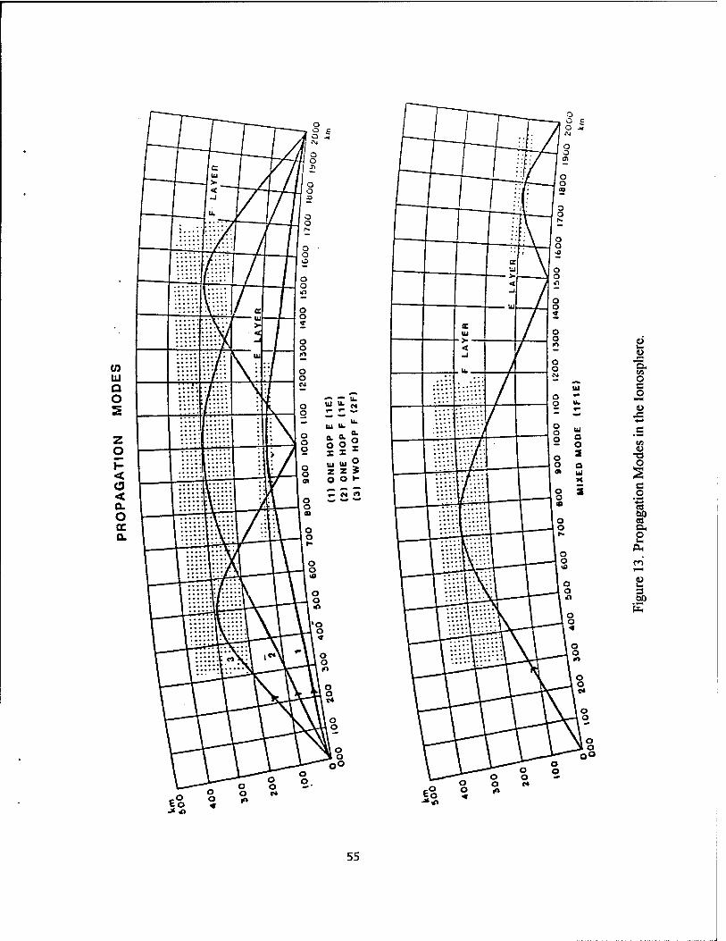
tu Q O
Z o <
< Q. O cc 0.
u.
::::::
b~r
/ tt r tu >
■ <
V. u
* ■ > • *
['.'.'.'.*•
N > y
:*.::: ::::':':
::::: •.:::*.:
::::: \:::'::
w u- N *- »■ w
■il:
\
1 U
E
LA
VP
R
tu
<
::::':
:::: '■.'::::■'■
:::.::
a. CO
O C o u
X!
O
c
eö 00 nj a. 2
PH
1—I
u. 3
55

RADAR CROSS SECTION OF A FULLY DEVELOPED SEA (Abel)
The strength of radar signals scattered back to the radar from the sea is the product of the
radar cross section per unit area of sea multiplied by the area illuminated by the radar. A fully
developed sea is one on which winds have acted for a time long enough to develop maximum wave
heights. These waves generally contain all possible wave components (wavelength components),
providing for a frequency independent scatterer. The radar cross section of the fully developed sea
for HF frequency range is roughly 0.005 to 0.001 square meter or in decibels -23 to -30 dBsm.
RADAR CROSS SECTION OF ICE (Abel)
The strength of radar signals scattered back to the radar from ice is the product of the radar
cross section per unit area of ice multiplied by the area illuminated by the radar. The radar cross
section of packed ice varies depending on the wind conditions and sea state when it was formed; on
the average, it is about 0.001 square meter (-30 dBsm) or one-tenth the radar cross section of a
folly developed sea. The radar cross section of glacial ice, such as that which covers Greenland, is
even smaller and is roughly one-hundredth that of a folly developed sea. Such a low cross section
shows a hole, on the screen display, over the Greenland area, within radar coverage.
RADIO WAVE POLARIZATION (Buchau)
Polarization defines how the electric field vector of an electromagnetic wave behaves. If the
vector stays within a plane, the wave is linearly polarized. If the vector oscillates in a vertical plane,
(at right angles to the direction of propagation) one speaks of a vertically polarized wave.
Correspondingly for a horizontally polarized wave, the electric field vector oscillates in a horizontal
plane. If the electric vector rotates at right angles with respect to the direction of propagation with
equal power in each direction of oscillation, the wave is circularly polarized. The polarization of a
radio wave is determined by the configuration of the transmit antenna. The transmit antennas (and
therefore the transmitted radio waves) and the receiver antennas of the ERS are linearly polarized.
The polarization of a radio wave and of the receiver antenna have to be matched in order to extract
the maximum power from the electromagnetic wave. An idealized antenna with horizontal
polarization will extract no power out of the field of a vertically polarized radio wave. (See also
Faraday Rotation).
56

RANGE FOLDING (Buchau/Abel)
The repetition of the radar waveform permits unambiguous measurement of a target's range
only up to the distance to which a radio signal can make a round trip within the time (period) x
between the start of two consecutive waveforms (x = 1/WRF where WRF is the waveform
repetition frequency). The maximum unambiguous range Rv is determined from the relation
R^ 0/(2 WRF) = C0T/2
with O the speed of light. A target at a range greater than Rv will appear range folded within R„ at
a range Ry given by
Rp = R-n Ru
with n an integer to be determined such that 0 < Rp < Ry. For example, for WRF = 40 Hz, x = .025
sec, Ru = 2025 nmi, a target at R = 2500 nmi range would appear range folded at RF = R-Ru = 2500-
2025 = 475 nmi.
RANGE (CLUTTER) RELATED NOISE (Sales)
Range related noise is a radar performance limiting phenomenon, which was first detected on
the FPS-95 OTH radar system in 1972. The term refers to the occurrence of an increased noise level
at the ranges where the ground clutter returns are strongest. As the ground clutter increased, the
noise level also increased, resulting in no improvement in performance even though more energy was
available to illuminate the aircraft targets. Although there is no universally accepted explanation of
this phenomenon, it certainly has the characteristics of an "area" effect. By reducing the illuminated
ground area (by reducing beam width and increasing range resolution, it was possible to reduce the
range related noise and yet not affect the detection of aircraft. Application of this concept to the
design of the current OTH systems has been successful. Range related noise does not limit the
performance of the AN/FPS 118 OTH radar to any significant degree.
RANGE RESOLUTION (Abel)
Range resolution is the ability of the radar to distinguish between two targets that are closely
spaced in range. Range resolution (RR) is determined from the relation RR = CJ(2 WBW), where C0
57

is the velocity of propagation (300,000 km/sec.) and WBW is the waveform bandwidth. For WBW
= 10 kHz, the range resolution is 15 km or 8.1 nmi. The actual radar resolution range is decreased
when the weight factors for the sidelobe reduction are applied, (the improvement ratio in sidelobe
reduction is between 1.2 to 2.4 for ECRS).
REFLECTION, IONOSPHERIC - see IONOSPHERIC REFRACTION
REFRACTION, IONOSPHERIC (Buchau)
In this physical process, radio waves start to bend upon entering the ionosphere, and continue
to bend until they bend back to earth, and thereby permitting the transmission of signals beyond the
horizon. More generally, refraction is the bending of a ray of light or other radiation, as it passes
from one medium to another of different refractive index. The refractive index is the ratio of the
phase velocity of light in free space to its phase velocity in the medium considered.
The refractive index of the ionosphere is a function of the electron density and the frequency
of the propagating wave, varying from 1 for free space to 0 for a plasma whose plasma frequency
is identical to the wave frequency of the propagating wave. For a plasma with a plasma frequency
greater than that of the wave frequency, the refractive index becomes imaginary, therefore the wave
will not propagate into such a medium and is reflected back. In the ionosphere, the refractive index
changes steadily with height, following the continuously changing electron density. This results in
continuous bending of an electromagnetic wave away from a layer maximum. If the radio wave
becomes horizontal prior to reaching the layer maximum, it will return to earth. If the radio wave is
still propagating upward at the layer maximum, it will penetrate the layer. In ionospheric
propagation, the term refraction is often loosely replaced by the term reflection. The general
principles of geometric optics and of reflection can often be used to quickly assess the propagation
modes, etc. However, it has to be understood that, in general, the process involved in returning radio
energy back to earth is that of refraction.
58

RELATIVE IONOSPHERIC OPACITY METER (RIOMETER) (Weber)
This is a sensitive radio receiver operating at HF and low VHF frequencies, used to monitor
the variation of cosmic radio noise that propagates to the surface of the earth. Most commonly 30
MHz is the operating frequency. Since the strength of this noise remains constant (for a given region
of the galaxy), variations measured at the surface of earth reflect changes in ionization density along
the signal ray path. A decrease in the received signal would result from absorption of the radio wave
energy by increased D region ionization. A network of riometers can thus monitor the spatial and
temporal characteristics of auroral absorption, upper atmospheric nuclear detections, and PCA
events.
S
SCATTER (Sales)
When radio waves encounter irregularities in the ionosphere or an irregular ground surface
(land, ocean waves), part of the energy is scattered in all directions from ionospheric irregularities
(isotropic scatter) and into the upper hemisphere from ground scatter. Energy scattered into the
direction of the incoming wave-front is called backscatter, since it propagates back to the radar. The
term clutter is synonymous to scatter. See also CLUTTER.
SIGNAL TO NOISE RATIO (S/N) (Sales)
In an OTH radar system, signal 'S' refers specifically to the energy returned from a small
(point) target (aircraft) in the radar's coverage. The detection of this "wanted" signal has to be made
against a background of noise ("N'). The total noise *N' is really a sum of internal noise, external
noise, and noise due to ionospheric clutter and interference. The relative amplitudes of the signal and
noise are given in terms of a simple ratio S/N.
SKIP ZONE/DISTANCE (Buchau)
For a frequency above the critical frequency of the F-layer, there is a maximum takeoff
angle, above which the radio wave will escape through the ionosphere and below which it will be
refracted back to earth. No energy of this frequency can propagate via the ionosphere into the skip
59

a 'B a Ö o
*-> *Ö c
c3
<U a o N & 3 C/3 U
X!
o c o 3 o o ►J
s
60

zone, the region between the transmitter and the landing point of the first refracted ray (Figure 14).
The skip distance increases as the critical frequency of the F-layer becomes lower, and decreases as
it goes higher. Also, the skip zone range increases with the upward movement of the reflecting layer
and decreases with the downward movement of the layer.
SOLAR ACTIVE REGION (Cliver)
A solar active region is a localized transient region of strong magnetic fields on the solar
surface in which flares originate. Active regions are composed of interspersed dark (sunspot) and
light (plage) regions. They typically have lifetimes < 30 days, but the largest active centers may
persist for several (5-6) solar rotations. Active regions rotate from east to west across the solar disk
with little variation in latitude.
SOLAR ACTIVITY CYCLE (SUNSPOT CYCLE) (Cliver/Coman)
The solar activity cycle is an 11-year period over which the number of spots on the sun, the
associated solar active regions, and the flares that emanate from these active regions, varies. The
rise of activity to a maximum, taking not more than 5 years, is slightly faster than the subsequent
decay to minimum (Figure 15). At the beginning of a cycle, near solar minimum, sunspots and
active regions form at relatively high solar latitudes, ~ 30°N and S. As the cycle progresses, the spots
originate closer and closer to the solar equator and by the end of the cycle, that is, just prior to the
next minimum, they typically form at 5°Nto 5°S latitude. Near solar maximum, sunspots and active
regions are distributed across the face of the sun in bands ~ 20°N and ~ 20° S of the solar equator.
At solar minimum, the solar surface may appear virtually spotless (and flareless) for periods of 1-2
years.
Since near each solar maximum the solar magnetic field changes its polarity (exchanges solar
North and South poles), one 11-year solar sunspot cycle is actually only one half of the 22-year solar
magnetic cycle. One may therefore find at times, the full solar cycle described as lasting 22 years.
Sunspot cycles have been numbered starting with number 1 in 1755. In July 1989 we passed the
maximum of the 22nd cycle. With a maximum sunspot number of R=159, this cycle was slightly
61

z D O U
>- _J i—i
er D
o Q_
z D CD
'-* V
■o ~o
CD
O o
:o .CM
- --'.-«*«?as
- '■»Xw*--?
— <***•'
= «*
T—I i I i • i ' '
'öde" '"oöz" ooi o- 006 oo3 y3aWHN lOdSNnS
-H-r ***-S
00 o\ 1—1
o VO I—I
00
•o o
•c <u PH u
JS *-> u
<2 ■2} "o >> U *-" o ca- t/a c 3
00 w-i
§>
62

higher than the median of the maximum values for the last six cycles. The solar minimum would be
in 1995-96 and the solar maximum would be in the next century.
SOLAR CYCLE see SOLAR ACTIVITY CYCLE
SOLAR FLARE (diver)
A solar flare is a rapid (T~< 60 min) release of electromagnetic (visible, radio, ultra-violet,
X-ray) and particulate (protons, electrons) energy from the sun. Flares are classified according to
the optically observed area of the solar surface covered, ranging from "0" for the smallest to "3" for
the largest, and their intensity, either faint (F), normal (N), or brilliant (B). The flares that cause the
most severe geophysical effects (that is, short wave fades, polar cap absorption events, geomagnetic
storms) are generally, but not always, of class 2B or greater. Solar flare X-rays produce the sudden
ionospheric disturbances (SID), of which the short wave fade is the most significant for the OTH
radar. During an SID the D region ionization is strongly enhanced, leading to partial or total
absorption of the radar's transmitted energy. The fading effect is strongest at the sub-solar point
and has a duration similar to that of the responsible flare, from minutes up to hours. Another
significant effect related to certain flares is the polar cap absorption event or PCA that is caused by
flare associated particles streaming in along geomagnetic field lines. This effect is most pronounced
in the strategically important polar cap regions and can persist for periods ranging from 10 hours to
4 days. Only the most extensive PCAs will affect the OTH radar, and only in their northernmost
sectors. Finally, flares can also be associated with coronal mass ejections, clouds of relatively low
energy particles and enhanced magnetic fields that arrive at earth 1-3 days after the flare and produce
the geomagnetic storm. Coronal mass ejections that give rise to geomagnetic disturbances are not
exclusively associated with large flares, but may also be associated with weak flares or disappearing
solar filaments Because of the effect of the interplanetary magnetic field on particle propagation,
energetic flares occurring on the western hemisphere of the sun are more likely to be followed by a
PCA effect than those on the eastern hemisphere. Geomagnetic storms are most likely to follow
flares near the central meridian while short wave fades may arise from flares anywhere on the solar
disk.
63
While a flare of any size may occur as often as once every two hours during the solar
maximum, the large geophysically significant flares occur at an average rate of <; 10 per year or about
once a month. Occurrence varies with the 11 year solar cycle and may be as low as one event at the
interval of several months ( could be even longer than a year) and as high as once every two days for
the geophysically significant flares when an important active region is on the visible disk.
SOLAR MAXIMUM (Cliver/Coman)
The activity peak in the smoothed (time averaged) eleven year solar activity cycle is defined
as the solar maximum.
SOLAR MINIMUM (Cliver/Coman)
The activity minimum in the smoothed (time averaged) eleven year solar activity cycle is
defined as the solar minimum.
SOLAR ROTATION (Coman/Cliver)
The sun rotates about its axis with an average period of 27 days. Because the sun behaves
as a fluid body, it rotates faster at its equator than near its poles. The period of rotation varies from
a minimum of 25 days at the equator to a maximum of 33 days near the poles. An active region will
be on the visible (from earth) hemisphere of the sun for about 14 days. If the region forms on the
back side of the sun, it will appear first at the eastern limb (edge) of the sun and rotate toward the
central meridian (0° longitude) and onward to the western limb at a rate of - 13° per day. If the
region is long-lived, it will reappear at the east limb ~ 27 days after its initial appearance. (Note that,
the 27 day rotation rates account for the recurrence interval between geomagnetic storms associated
with coronal holes.
SOLAR WIND (Weber/Buchau)
This is an ionized gas (plasma) flowing outward from the sun, dragging along field lines of
the solar magnetic field, away from the sun along the Interplanetary Magnetic Field (IMF) lines. The
solar wind consists of high speed flows from coronal holes, steady slower flows associated with
64

coronal streamers, and transient flows of coronal mass ejections. The solar wind exerts pressure
on the earth's magnetic field to form the magnetosphere. The solar wind particles (mainly electrons
and protons) enter the magnetosphere and at some later time precipitate into the atmosphere resulting
in aurora and particle produced ionization. The arrival at earth of high speed co-rotating streams
or of coronal mass ejections and its preceding shock wave can cause a geomagnetic storm. Of
importance to the estimate of the geomagnetic effects of high speed streams and coronal mass
ejections are the velocity of the plasma, the field strength of the IMF and its direction at the time of
arrival at the boundaries of the magnetosphere.
SPECTRUM ANALYSIS (Buchau/Sales)
It can be shown that any signal can be thought of as being composed of an infinite series of
harmonically related frequencies of different amplitudes. This is obvious for a signal which initially
has been composed of discrete frequencies and their respective amplitudes, and which as a sum will
reproduce a given signal. Spectrum analysis is the decomposition of a signal into its sinusoidal
components.
One important signal is the mixture of ground clutter, noise, and target signal available at
the output of the OTH radar receiver. The ground clutter arriving from the same range as the target
(aircraft) is some million (one million= 60 dB) times larger than the return from the target. For this
reason detection would be impossible, unless advantage is taken of the fact that the aircraft returns
are Doppler shifted by an amount proportional to the radial speed of the aircraft while the clutter
has the exact frequency (zero Doppler) of the transmitted signal. Spectrum analysis permits the
separation of the ground clutter at 0 Hz Doppler from the signal returned by an approaching or
receding aircraft and therefore permits the detection of an aircraft. If noise energy with the same
spectral (frequency) component as the target Doppler exceeds the target signal level, the OTH system
will experience problems in detecting and/or tracking of the aircraft.
Spectrum (Fourier) analysis is a mathematical process that makes it possible to decompose
the digitally sampled received radar signal into the separate frequency components that make up the
complex received signal. In general, a received signal consists of the ground clutter return, noise, and
possibly target signals. Each of these components has a different frequency composition. Those
65
components that originate from the radar transmission, such as the ground clutter and the target
signals, are narrow band (even though the transmitted waveform has a nominal 10 kHz bandwidth)
since the digital sampling at the output of the receiver (one sample per waveform repetition) makes
these signals appear as a CW signal with a finite duration equal to the CIT. For CIT= 1 s, the
bandwidth of the spectrum processing is only 1 Hz. This means that these coherent signals appear
in a single frequency (Doppler) cell. The very strong ground clutter signal backscattered from land/
sea typically falls into the zero Doppler frequency bin while a moving aircraft target with Doppler
shifted returns, which are considerably weaker than the ground clutter return (often 60 dB below the
ground clutter), can be easily recognized (detected) because they fall into one of the unoccupied bins.
On the other hand, the noise signal is not coherent with the radar transmissions and the spectrum
processing divides the total noise power relatively uniformly over all the frequency bins of the
spectrum. The number of frequency bins is equal to the number of waveform repetitions in the
coherent dwell time (CIT). This distribution of noise power over all the Doppler bins while at the
same time the target signal falls into one frequency bin, results in an improvement by a factor of N
(number of bins) in the target to noise (power) ratio.
SPECULAR SCATTER (Sales)
In contrast to field aligned or orthogonal (perpendicular) scatter, specular scatter requires
a different ray path for the returning signal than the one followed out from the transmitter. Specular
scatter is strongest when the angle of incidence of the outgoing radar signal on the irregularity equals
the angle of reflection (for the returning scattered signal). This condition tends to be more difficult
to satisfy in the ionosphere than the requirement for orthogonality.
SPORADIC E O8*1)
In contrast to the regular solar produced E-layer in the height range between 95 and 130 km,
which has a half thickness of 25 to 35 km, the transient sporadic E (Es) is a layer of ionization with
a thickness of only a few kilometers. Unlike the meteor trails, which last only for seconds, the
lifetime of Es is many minutes to many hours and the size of Es-patches is several hundred kilometers.
66

It is probably caused by wind shears that sweep metallic ions from the top and bottom ofthat region
into a small height range of one half to two kilometers.
At mid-latitudes Es is typically a summer phenomenon with an occurrence probability of >
70% around noontime. Auroral Es related to particle precipitation and intense currents (auroral
electrojet) can be observed with high (> 70%) probability within the auroral oval, independently of
season and time of day.
SPREAD F (Basu)
The ionospheric phenomenon that gives rise to a diffuse ionogram trace for frequencies
reflected from the F region is known as Spread F. Spread F has been classified into two types: (1)
frequency spread F when the spread is near the critical frequency of the F layer and (2) range
spread F when the spread is over the horizontal part of the trace. The phenomenon arises as a result
of the scattering of radio waves from ionospheric irregularities and is observed most frequently
during both day and night at high latitudes and only during nighttime hours at equatorial latitudes.
During geomagnetic disturbances, it can also be found at mid-latitudes.
STORM SUDDEN COMMENCEMENT (Coman)
A Storm Sudden Commencement (SSC) is a rapid increase in the horizontal component of
the geomagnetic field lasting about 1 to 6 minutes and appearing simultaneously world-wide. It
normally indicates that an intense geomagnetic storm will follow. An SSC results when the shock
wave driven by a coronal mass ejection (CME) strikes and compresses the sunward magnetosphere.
The main phase of the storm begins (ensues) when energy contained in the magnetic field of the CME
is transferred to the magnetosphere by reconnection of field lines.
SUDDEN IONOSPHERIC DISTURBANCE (SID) (Coman)
This is a sudden simultaneous increase in the electron density of the ionosphere over the
entire day side hemisphere. The SID is caused by the sudden increase in solar x-ray flux associated
with energetic solar flares. The increased ionization normally occurs in the D region of the
67
ionosphere and may last from a few minutes to several hours. Long range radio propagation is
affected by absorption, frequency deviations, and signal phase and amplitude changes.
An SID normally falls into one or more of the following categories:
1. Short Wave Fade (SWF)
2. Sudden Cosmic Noise Absorption (SCNA)
3. Sudden Enhancement of Atmospherics (SEA)
4. Sudden Frequency Deviation (SFD)
5. Sudden Phase Anomaly (SPA)
SUNSPOTS (Coman)
These are dark areas (or spots) that appear in the photosphere of the sun. These regions
appear dark because they are cool relative to the surrounding photosphere. Sunspots have been
found to be regions of strong localized magnetic fields. Most features of solar activity occur in
regions surrounding sunspots.
SUNSPOT NUMBER (Coman)
It is an internationally accepted measure of the level of solar activity. The relative sunspot
number (also known as the Wolf number) is given by:
R = K(10g + n)
where n is the total number of individual spots, g is the number of sunspot groups, and K is a
correction factor to account for systematic differences between observing stations.
T
TERMINATOR (Moore)
The terminator is defined to be the border between sunlight and darkness or the boundary of
the earth's shadow. Ionization due to incident sunlight ceases when the ionosphere enters the dark
region bounded by the terminator (that is, the earth's shadow).
68

TRAPPED MODE (Coman)
In radar theory, this is one of several modes in which electromagnetic waves can propagate.
This mode is characterized by radio energy being confined between refractive index boundaries
(similar to material boundaries of a wave guide) that represent a duct.
In the ionosphere, such a duct forms between ionospheric layers (or on the underside of one
layer: chordal mode), which can confine radio waves and result in abnormally long transmission
ranges (for example, round-the-world signals) because of reduced spreading as well as reduced losses
at ionospheric altitudes where electron-neutral and electron-ion collisions are small. Excitation of
trapped modes over a particular ground-based propagation link is intermittent. While trapped radio
signals can be propagated over large distances at low loss, their illumination of a particular
surveillance area cannot be guaranteed. Moreover, associated field strength fluctuations may be large
and delay-time to ground-range conversion is uncertain. The favorable horizontal gradients required
to facilitate injection of ducted modes are associated with the sunrise and/or sunset terminator. The
occurrence of these modes and the resulting interference with conventional modes is believed to be
of minor importance. However, strong horizontal gradients associated with the high latitude
ionosphere are, for extended periods, a possible entry region for ducted modes. The existence of
these modes, however, has not been proven. If the trapped mode encounters ionospheric
irregularities (especially at right angles), energy will be scattered back toward the transmitter.
Because of the low losses and reduced spreading, it is possible that ionospheric clutter from large
ranges may be effective in interfering with the radar.
TRAVELING IONOSPHERIC DISTURBANCE (TU)) (Coman)
Atmospheric gravity waves originating at the auroral oval or at the terminator travel at speeds
of 1000 km/hour over the earth's surface. Due to interaction between the neutral atmosphere and the
ionosphere, they result in temporary enhancements and depletions of the ionosphere that travel with
the gravity wave, therefore their name Traveling Ionospheric Disturbances. An OTH radar beam will,
during the transit of a TID across the midpoint ionosphere, experience a sudden lowering of the
reflection height, resulting in a change of the location of the barrier. These changes lead to variations
of the observed aircraft Doppler and to discontinuities in aircraft tracks.
69

u UNIVERSAL TIME (UT) (Weber)
The Greenwich or prime meridian (0° longitude), is the reference meridian for the geographic
coordinate system and local time along this meridian is called Universal Time. The principal use of
UT is to provide a standard 24 hour time coordinate that applies to the entire globe. Thus, global
events can be related by their temporal development measured in UT. Local time is related to UT
by a time advance of 1 hour/150 of East Longitude or a delay of 1 hour/150 of West Longitude..
VERTICAL INCIDENCE - see INCIDENCE, VERTICAL
VIRTUAL HEIGHT (Dandekar/Buchau)
The virtual height is the apparent height of reflection for a given HF frequency from a vertical
sounding of the ionosphere. It is given by C0t/2, where C0 is the velocity of light and t is the time
delay between the sending and the reception of the radio waves. Due to the retardation (slowing
down) suffered by radio waves in the ionosphere below the reflection level, the virtual height is larger
than the true height of reflection. For oblique propagation, the virtual height of reflection is that
height that can be computed from the signal travel time, assuming that the. radio wave travels with
the free space velocity of light and assuming a ray path following the laws of geometric optics
(straight lines). The virtual height of reflection of an operational frequency can be determined from
an ionogram recorded at the midpoint of the propagation path. This concept provides for the
generation of the coordinate registration (CR) tables. The virtual height thus established permits the
conversion of radar range (travel time of a radar signal from transmitter to target back to receiver)
into ground range distance.
70
w WAVEFORM BANDWIDTH (Abel)
The waveform bandwidth is the width of the radio frequency (RF) spectrum occupied by a
transmitted signal. If the signal waveform contains frequencies between a lower limit fx and upper
limit f2, the waveform bandwidth is equal to the difference between fj and f2. For example, a
waveform containing frequencies between 20.020 MHz and 20.030 MHz has a bandwidth of 0.01
MHz or 10 kHz.
WAVEFORM REPETITION FREQUENCY (WRF) (Abel)
Waveform repetition frequency (WRF) is the number of times per second that the modulating
waveform is applied to the transmit (center) frequency. For example, for a WRF of 20 Hz, the
waveform is repeated 20 times during each second.
Z
ZENITH ANGLE (Moore)
The zenith angle of a point is the angular distance from the zenith of the observer to the point
measured along the vertical circle through that point.
71

72

Bibliography
Air Force Global Weather Central, (1982), Source Book of the Solar-Geophysical Environment,
Space Environmental Course, Third Edition, AFGWC/WSE, OFFUT AFB, NE 68113.
Jursa, A. S., Scientific Editor (1985), Handbook of Geophysics and Space Environment, Air Force
Geophysics Laboratory, National Technical Information Service number ADA 167000.
Lloyd, J. L., Haydon, G. W., Lucas, D. L., and Teters, L. R., (1978) Estimating the Performance
of Telecommunication Systems Using the Ionospheric Transmission Channel, National
Telecommunications and Information Administration, Boulder, Colorado.
Phase II Training Modules (for OTH-B Radar Operators), Vol I, The Environmental Assessment
Training Manual, VolJL, Detection/Tracking Module, Voim, Radar Control Training Manual, and
Vol IV, Track Correlation Training Module.
Sales G, (1992), High Frequency (HF) Radio-wave Propagation, PL-TR-92-2123, (chapter 4 of the
OTH-B Handbook), ADA261726.
Sales G, (1992), OTH-B Radar System: System Summary, PL-TR-92-2124, (chapter 2 of the OTH-
B Handbook), ADA261727.
73


![15 Sediment Gages - USGS · 0.2707 c,S372 Velccty and backscatter seres C] Depth-averaøed streamwise vebcfy RMS Curr.tive u at depths backscatter Depth-averaged backscatter Contour](https://img.pdfslide.us/doc/110x75/5fd8133cbc6723794903cbd2/15-sediment-gages-usgs-02707-cs372-velccty-and-backscatter-seres-c-depth-averaed.jpg)

![UWB Radars [EDocFind.com]](https://img.pdfslide.us/doc/110x75/577d2b9c1a28ab4e1eaae39f/uwb-radars-edocfindcom.jpg)