Global Trade Analysis Project (GTAP) - Examining the India, Brazil … · 2007-08-28 · 1 Summary and general conclusions from the analysis Following a comprehensive examination

Examining the India, Brazil and South African (IBSA) Triangular

Trading Relationship

by

Ron Sandrey and Hans Jensen

tralac Working Paper No 1/2007

February 2007

Copyright © tralac, 2007.

Readers are encouraged to quote and reproduce this material for educational, non-profit

purposes, provided the source is acknowledged. All views and opinions expressed remain

solely those of the authors and do not purport to reflect the views of tralac.

This publication should be cited as: Sandrey, R. and Jensen, H.

2007. Examining the India, Brazil and South African (IBSA) Triangular Trading Relationship

tralac Working Paper No 1. [Online]. Available: www.tralac.org

tralac acknowledges the funding support of AusAID for this publication.

1

Summary and general conclusions from the analysis

Following a comprehensive examination of the most recent merchandise trade flows

between the relevant countries this paper uses a computer model to look at the possible

economic results from removing all merchandise1 tariff barriers between the three partners of

India, Brazil and South Africa/SACU. We have ignored the political complication of Brazil

also belonging to a free trade agreement and we have not modelled the estimation and

removal of non-tariff barriers, services trade or some of the more sophisticated but

speculative gains from technological change or other dynamic effects. Recent research,

some of which is cited in the paper, has highlighted that most of these fancier assumptions

are misleading to policy makers.

The IBSA agreement is potentially good for all major parties with similar welfare gains of

between one to one and a half billion dollars at 2015, but with this translating into larger

gains for South Africa when measured as a percentage of real GDP as South Africa has a

smaller economic base to work from. The gains to South Africa are spread across the

contributing factors of allocative efficiency, labour’s contribution, capital and the terms of

trade gains from both (a) better relative prices between exports and imports and (b) more

efficient use of capital. The biggest loser in dollar terms is the EU, with all other

countries/regions except Nigeria losing. Unfortunately these losers include both Botswana

and ‘rest of SACU’ or the model aggregation of Lesotho, Namibia and Swaziland combined,

although these losses are not high and may be misleading given that intra-SACU trade and

therefore any changes in this trade will not be picked up in the model’s database given the

poor quality of this trade data.

Another feature of the analysis is that we have used as our base for the simulation a trade

picture that includes all the known global updates, and this includes simulating the effects of

the Trade, Development and Cooperation Agreement with the EU in such a way that enables

us to isolate these effects from the base. Results from this TDCA simulation suggest that a

full and comprehensive IBSA FTA is of greater value (in fact about double the welfare gains)

to South Africa than the partial TDCA as it now stands. This is mainly because (a)

South Africa faces manufacturing tariffs that are modest, thus the preferences are not that

significant, and, more importantly, (b) South Africa gains little preference into the highly

protected European agricultural market from the TDCA. Conversely, for IBSA, South Africa 1 We have used the interchangeable terms of ‘merchandise’, ‘goods’ and ‘products’ either together or separately in this paper. They generally refer to the actual physical items that are traded. The celebrated definition from the Economist magazine is that these are items that hurt when dropped on your foot, and the terms are used to preclude the trade in services.

2

is deemed to have gained comprehensive access into the relatively highly protected Indian

market, thus gaining a considerable advantage over global competitors in both agricultural

and non-agricultural goods.

In the first section of the paper we examine the current trade flows between the IBSA

partners and hypothesise that the interesting results for South Africa may concentrate upon

the sugar trade in agriculture and the motor vehicle trade in the non-agricultural sectors.

Neither of these proved to be significant for South Africa. Sugar production actually declines

in South Africa despite gaining better access into India, as this access is taken up by Brazil

rather than the presumably less efficient South African production. Similarly for motor

vehicles, where South African production declines by 1.6 percent in the face of more efficient

production and consequently imports from Brazil in particular and to a lesser extent India.

Given the extent to which China has displaced South African domestic production of clothing

with its dramatically increasing exports over the last few years, it should be no surprise that

India, although currently not a major source of South African imports but a country with

enormous production capacity perhaps second only to China, should compete strongly in

South Africa if tariffs were to be eliminated. Clothing production declines by 8.7 percent, and

this is a massive decline for an individual sector2.

However, the major finding from this GTAP exercise, and one not anticipated from the trade

data, is the massive gains to South Africa from attractive access into India from a zero rather

than 15 percent duty on gold. This is a happy juxtaposition on the world’s leading gold

producer meeting a large jewellery exporter that enables both partners to prosper as India’s

costs are reduced. Indeed, it is this sector that is driving a considerable portion of the welfare

gains to both South Africa and India, and the policy implication is very clear: reducing the

Indian tariffs on gold is a win-win situation and must become a priority for negotiators.

Another major finding from this GTAP work is related to the employment closures, where the

trade-offs between holding wages constant and increasing the supply of unskilled workers at

one extreme and, conversely, holding the supply of workers constant and increasing wages

are clearly demonstrated. The somewhat intermediate position of allowing the unskilled

labour increase to be a function of the unemployment rate in each country has been adopted

as the standard closure for the model, with these two extremes and another closure that

2 Sandrey (2006c) in discussing the trade and economic implications of the South African restrictions regime on the imports from China provides extensive background to the background on the clothing imports into South Africa.

3

holds wage rate increases for unskilled workers to be in line with the inflation rate. There is

no doubt that holding wages down and reflecting as much of the change in increasing

unskilled workers entering the labour force is the best policy for South Africa. This increases

welfare and lessens inflationary pressures quite substantially.

We have provided three alternative scenarios to judge the full and complete removal of

merchandise tariffs. These are (a) a 50 percent tariff reduction rather than the full

100 percent, (b) a realistic Doha Round agreement, (c) a full 100 percent IBSA simulation

post-Doha. Results for (a) show that this gives 43 percent of the gains for South Africa and a

lesser 30 percent for Brazil but is much better for India who maintain 62 percent of their full

gains as the relative prices move around and consequently the trade outcomes are not a

linear 50 percent. Results for (b) show that gains from a possible Doha agreement are

extremely modest for agriculture in particular for all parties once special and sensitive

exemptions are made to tariff reductions globally. However, much larger global gains in non-

agricultural sectors (NAMA) compensate for this disappointing agricultural outcome for South

Africa. Results from (c) show that since the Doha results are modest, their diminution of the

original IBSA 100 percent results are similarly modest for South Africa.

Results for the agricultural sector are modest. Initial agricultural products have been a very

minor part of South Africa’s exports into India’s heavily protected market, while agricultural

imports from India are concentrated in the duty-free imports of rice. Brazil has become a

major global player in agricultural exports, and sends large quantities of soybean products

and poultry meats, pork and beef to South Africa. Following the FTA South Africa increases

exports to India by $184 million and Brazil by an insignificant $7 million. Overall some

$144 million of the increase is trade diversion from previous destinations and leaves a global

increase of only $46 million overall. Increases are in vegetable oils and fats ($69m) and wool

(29m) to India take place, while there are global reductions in exports of (a) vegetables, fruit

and nuts and (b) other food products. For imports, there is a similar but slightly larger

overall increase of $93 million, driven mostly by increased imports from Brazil of $75 million

(other crops, other meats and vegetable oils and fats).

The implication for the BLNS countries of Botswana, Lesotho, Namibia and Swaziland are

disquieting, as they see declines in their welfare. This mostly comes from terms of trade

losses as the better access for South African non-agricultural goods into India consequently

increases the relative prices for SACU imports from South Africa. Exports of sugar products

(we presume from Swaziland) to India increase, but this is mostly at the expense of reduced

exports to the EU overall. Exports from Botswana reduce marginally in the manufacturing

4

sector as their costs increase (but also marginally). Imports from India increase, but almost

all of this is a substitution away from the traditionally-based South African source. There are

very low and insignificant changes in the trade flows with Brazil. In agriculture, there are no

(or almost no) changes to trade flows other than the sugar exports to India.

Finally, we undertake some alternative scenarios around the unskilled labour market closure

assumptions in the primary model. We expand from the standard assumption that

employment is fixed and the adjustment is through the wage rate to use the closure whereby

unskilled labour supply is a function of the unemployment rates in each country and the

adjustment therefore varies between changes in employment and the wage rate depending

upon that initial unemployment rate. We also simulate a scenario where the closure has the

real wage fixed and all adjustments must come through the number of unskilled persons

employed. Here the results are striking: employment is up by 2.84 percent, welfare more

than doubles from the primary model results to $3,015 million and inflation is a significantly

lower 0.47 percent. This dramatic result clearly highlights that if South Africa is serious about

increasing both welfare and employment in the economy, the more policies move towards

creating jobs rather than rewarding those actually in employment is a superior option for

policy makers.

Introduction and background

In recent months the question of a closer trading relationship between India, Brazil and South

Africa (the three IBSA partners) has occupied a lot of media attention. The objective of this

paper is to focus upon the current merchandise trade and place this in perspective for a more

cooperative approach. The analysis will extend to undertaking an advanced computer

general equilibrium modelling study to assess what the gains may be from a trilateral free

trade agreement (FTA) between the partners. The paper will note here at the beginning that

such an FTA is conceptual only, as both Brazil and South Africa are members of their own

FTAs (Mercosur and SACU respectively) and a country cannot be a member of more than

one Customs Union. Nonetheless, an FTA sets the outer boundaries for an enhanced

trading regime, and in recognition of South Africa’s membership of SACU we will consider

the implications of the IBSA agreement for the fellow SACU members of Botswana, Lesotho,

Namibia and Swaziland (BLNS). All data in this first section of the paper is sourced from the

commercially available World Trade Atlas3 (Dr John Brasher), which is in turn sourced from

the official country sources.

3 World Trade Atlas at www.gtis.com.

5

The analysis will concentrate upon using the respective partners’ import data, as this is

generally more reliable than export data. Two points must be made here, though. The first

is that imports are usually assessed using CIF (the value of the goods plus the costs of

freight and insurance transporting them from the export dock to be unloaded at the import

border) while exports are assessed as FOB (free on board, or the actual value of the goods

at the export dock). This means that we are in effect inflating the import value as compared

with the export value by including freight costs, and in the case of some bulk products, this is

significant. However, importantly we note that South Africa is one of the few countries in the

world that both reports on and assesses duty for imports without adding the costs of

shipment and insurance. The second point is that export and import values seldom if ever

agree, and we will introduce a reconciliation exercise to explore some reasons for this, with

the CIF versus FOB values just one reason. All data is expressed in US dollars.

Overall all three partners share important and somewhat equal trading relationships.

Firstly, South Africa’s major exports to the world are concentrated in minerals and related

products. The major global exports by the general HS 2 Chapter4 has been precious metals

and stones etc. (platinum, gold and diamonds), followed by iron and steel products, mineral

fuels and motor vehicles, and these four products made up 55.6 percent of the total exports

during 2005. The main export to India during 2005 was the one-off aircraft, followed by

inorganic chemicals, iron and steel products and again precious metals and stones. These

top four accounted for 65.5 percent of the total South African exports to India, and in addition

we would note that Indian import data shows that precious stones, metals and minerals etc

may be under-reported in the export data as South Africa does not generally disclose its

export destinations for gold. Our analysis suggests that these exports face an average tariff

of some 15.88 percent using Indian import data. The main exports to Brazil were iron and

steel, organic chemicals, general machinery and mineral fuels, with these four comprising

63.3 percent of the total. Again, tralac analysis suggests these products faced an average

duty of 8.95 percent during 2005, and that the proposed SACU/Mercosur FTA would make

little difference to this rate.

4 Where HS is the Harmonised System of merchandise trade classification that operates in a sequentially more detailed level from internationally harmonised (hence the name) HS 2 to 4 and 6 levels, and often down to even HS 10 for individual countries. For example, the HS6 classification scheme contains about 5000 product groups, and this and often more detailed levels are used for specifying tariff schedules.

6

Secondly, India’s main exports to the world are precious metals and stones, mineral fuels,

clothing and organic chemicals, with these four making up a lesser 36.3 percent of the total.

There is a direct linkage between India’s exports of precious jewellery and South Africa’s

base metal exports, as India has become the main processing and trading centre globally for

these often South Africa-sourced raw materials. Exports to South Africa were concentrated

in mineral fuels, vehicles, cereals and iron and steel products, with these exports making up

52.9 percent of the total. Indian exports to Brazil were mineral fuels (49.6% of the total),

organic chemicals, pharmaceuticals and miscellaneous chemical products, with the top four

comprising 71.3 percent of the total.

Finally, Brazilian global exports are even more diversified than India’s, with the top four of

vehicles, machinery, iron and steel and ores, etc., comprising 32.0 percent of the total.

Exports to South Africa are concentrated in vehicles and parts (31.8%), machinery, meats

(poultry) and sugars. In fifth place is soybean oils and in sixth place is tobacco, reaffirming

the importance of Brazil for South African agricultural imports. Exports to India feature

sugars, soybean products, aircraft and beverages, with these making up 63.2 percent of the

total. In agriculture, Mercosur in general provides around one-quarter of the global imports,

and Brazil is highly competitive in the crucial beef, pig meat and poultry sectors with all three

(along with sugar cane) receiving virtually no government supports.

It is noticeable that iron and steel products and vehicles and their associated parts feature in

the top four global exports from both Brazil and South Africa, and these are ranked sixth and

eighth respectively from India. There appears to be a degree of intra-industry trade among

the three partners in these products as well, leading to the general conclusion that the gains

from cooperation here may not necessarily be in ‘new’ trade but more sophisticated linkages

in existing products. Brazil, as a major agricultural exporter, will remain a valuable source of

both food for direct consumption in South Africa and imports such as the soybeans to provide

the feedstuffs for the livestock sector.

The automobile sectors

Of particular interest to South Africa has to be the automobile sector, where the new

international ‘buzz word’ acronym is ‘BRIC’ for Brazil, Russia, India and China. Analysts

consider that the biggest breakthrough in global growth will come from these BRIC countries.

They will shortly account for more than 40 percent of forecast global light vehicle assembly

increases and represent around half of the industry’s forecast global capacity expansion.

Consequently, nearly all major global automakers are pursuing a BRIC strategy in some form

7

as they attempt to gain competitive advantage by linking a presence into these emerging

markets5. South Africa could be poised to gain an advantage over several competitors

should some form of preferential and cooperative trading agreement be formulated between

IBSA.

The Brazilian sector in particular is very competitive, with excess capacity, high rates of

taxation and interest and a weakening consumer demand. However, its technology in the

flex-fuel engines which run on gasoline, ethanol or any blend of the two is likely to create a

huge demand for this technology should global oil prices stay high. Similarly, India’s annual

automobile sector growth has been the highest in the world in recent years, with this

accentuated by the shift in automobile production from the US and Western Europe to Asia,

with India and China taking the lead. Consequently, India has become the largest

manufacturer of tractors in the world, the second largest manufacturer of three-wheelers and

two-wheelers, third largest manufacturer of commercial vehicles, and fifth largest

manufacturer of cars. International companies are scrambling to establish themselves in this

market in particular, and that presence includes establishing design and research centres in

addition to India’s more traditional lower cost production.

The agricultural sectors

Since the early 1990s India has undergone considerable economic policy reform, although

agricultural reform has lagged behind other sectors. The general pattern of agricultural

protection (as measured by the Producer Support Estimate (PSE)) is for support to rise when

world prices are low and decline when they are high, making analysis very complex.

Depending upon the method used to calculate these PSEs, they were near their highest in

2002 at 11.0 to 19.2 percent overall, while in 1996 they were negative (i.e., taxing the sector)

at similar rates.

Agricultural exports have been a very minor part of South Africa’s exports to India; during

2005 they were some 1.8 percent of the South African exports to India, a similar figure to

2003’s 1.9 percent but below the 2004 figure of 3.5 percent when a larger export of sugar

was made. Indeed, some 87 percent of the agricultural exports during 2005 were either

sugar (50.2%) or wool (36.8%), while fresh fruits and cotton provided another 4.7 percent

and 2.0 percent respectively. This pattern has changed little over the last ten years. Sugar

appears to have potential for increased imports from South Africa under a less distorted

5Downloaded from http://www.pwc.com/Extweb/ncpressrelease.nsf/docid/7C7BE1A291BB6BD5852572040082059C.

8

regime, notwithstanding the fact that India is the world’s second largest producer of sugar

after Brazil with around 15 percent of the global production. Between 2001 and 2003 India

was a large exporter of sugar, but in 1999, 2004 and 2005 it has been an importer. Brazil is

certainly more internationally competitive in sugar than India and even probably South Africa.

Meanwhile, India’s sugar regime is highly regulated, with an import duty of 100 percent plus

a possible countervailing duty of another 850 rupees per ton, the sugar levy obligations, the

sugar release quota system and other domestic regulations. Thus, there seems to be some

scope for cooperation in this agricultural market in particular.

Brazil has virtually replaced Australia as the international champion for agricultural free trade

globally. Its potential is enormous, with good land exceeded only by China, the US and

Australia and a policy regime that has both contributed to and benefited from the radical

economic reforms in Brazil over the last 15 years. Support to the sector is now minimal (PSE

of around 3%, a figure even lower than South Africa’s and not much above the radical

agricultural reformers of New Zealand and to a lesser extent Australia). Overall production

has similarly increased following the economic reforms, with technological change a key

driver in this expansion, an expansion that has recently lead to concerns about the

environmental consequences of agriculture moving into new lands. Brazilian agricultural

exports have increased to the extent that they are now around 30 percent of total exports,

and they moved dramatically away from the traditional tropical products of coffee and orange

juice to being major global suppliers of soybeans, sugar and the grain-soybean feed for

meats of chicken, beef and pork.

The structure of the paper is as follows. The first section will examine the current bilateral

relationships sequentially, starting with (a) South Africa and India before examining (b) South

Africa and Brazil and then (c) Brazil and India. A similar format will be followed for each of

the three sectors, with analysis on current and recent merchandise trade flows that reports

on assessed tariffs, growth rates and market share to put this trade in perspective before

starting to examine the future with a ‘trade chilling’ analysis of potential trade products based

on the current trade patterns for the respective partners. The second section of the paper

will use the Global Trade Analysis Project (GTAP) international computer model to simulate

the impacts of an FTA between the partners under different scenarios. The final section will

compare and contrast sections one and two before making some general conclusions.

9

Section One: The trading relationships The big picture

These three countries are emerging globally in that Brazil and India have both become

crucial players in the world trading arena while South Africa is the important ‘bridge’ between

the developed world and developing Africa. In terms of economic power, the World Bank

ranks Brazil 10th, India 12th and South Africa 27th by traditional GDP, but all are higher by

the more useful Purchasing Power Parity (PPP or what your money will buy) index. As a

measure of import openness, Brazil collected import duties equivalent to 8.4 percent of total

merchandise imports, while the similar figures for India and South Africa were 14.1 and

2.7 percent respectively. Thus South Africa could be regarded as being very open on

average (with motor vehicles and clothing distorting that average) while India is relatively

highly protected. Brazil is a major agricultural exporter with one-third of its total exports

classified as agriculture (compared to India at 11.3% and South Africa at 7.9%), while

agricultural imports range between 6.2 to 7.0 percent in all three cases.6

All three partners are also part of what may be described as ‘second rung’ trading nations,

and all rank relatively closely together, with world ratings between 24th for both Brazil in

world exports and India in world imports and 37th for South Africa in world exports.

Examining the World Trade Atlas data shows global exports from Brazil, South Africa and

India of $118 billion, $52 billion and $100 billion respectively during 2005, and similarly

imports of $74 billion, $55 billion and $138 billion for the same countries. An analysis of the

WTO Annual Report shows very similar but not always identical data; for South African

imports, for example, the WTO reports $67 billion rather than $55 billion. We would

hypothesise that the difference is that the World Trade Atlas does not report intra-SACU

trade for South Africa. Table 1 shows the general trading relationships between the three

countries, along with the bilateral rankings based upon individual destinations/sources (i.e.

with the EU countries ranked on their own). The data confirms that the respective partners

are (in not a derogatory manner) ‘second rung’ but still important trading partners ranging

from 11th for South African imports from Brazil to 36th for Brazilian imports from

South Africa.

6 WTO at www.wto.org.

10

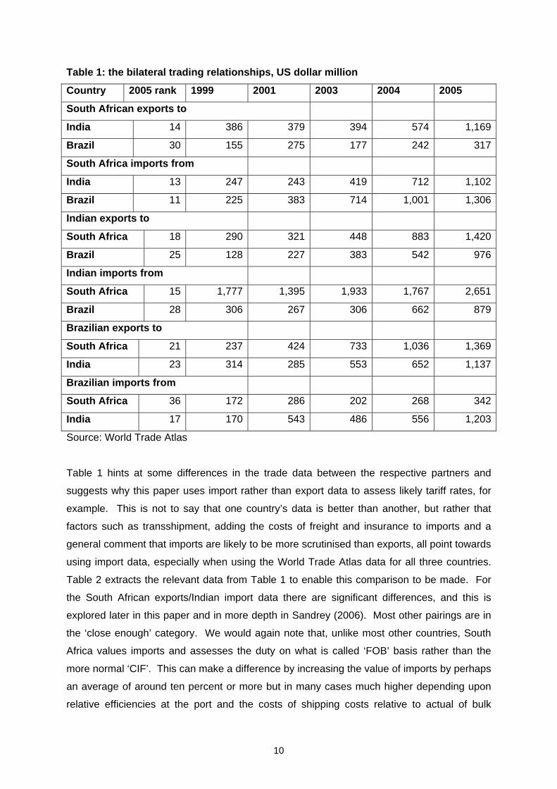
Table 1: the bilateral trading relationships, US dollar million

Country 2005 rank 1999 2001 2003 2004 2005

South African exports to

India 14 386 379 394 574 1,169

Brazil 30 155 275 177 242 317

South Africa imports from

India 13 247 243 419 712 1,102

Brazil 11 225 383 714 1,001 1,306

Indian exports to

South Africa 18 290 321 448 883 1,420

Brazil 25 128 227 383 542 976

Indian imports from

South Africa 15 1,777 1,395 1,933 1,767 2,651

Brazil 28 306 267 306 662 879

Brazilian exports to

South Africa 21 237 424 733 1,036 1,369

India 23 314 285 553 652 1,137

Brazilian imports from

South Africa 36 172 286 202 268 342

India 17 170 543 486 556 1,203

Source: World Trade Atlas

Table 1 hints at some differences in the trade data between the respective partners and

suggests why this paper uses import rather than export data to assess likely tariff rates, for

example. This is not to say that one country’s data is better than another, but rather that

factors such as transshipment, adding the costs of freight and insurance to imports and a

general comment that imports are likely to be more scrutinised than exports, all point towards

using import data, especially when using the World Trade Atlas data for all three countries.

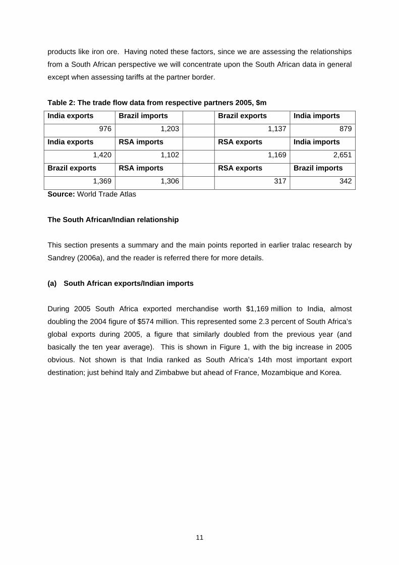
Table 2 extracts the relevant data from Table 1 to enable this comparison to be made. For

the South African exports/Indian import data there are significant differences, and this is

explored later in this paper and in more depth in Sandrey (2006). Most other pairings are in

the ‘close enough’ category. We would again note that, unlike most other countries, South

Africa values imports and assesses the duty on what is called ‘FOB’ basis rather than the

more normal ‘CIF’. This can make a difference by increasing the value of imports by perhaps

an average of around ten percent or more but in many cases much higher depending upon

relative efficiencies at the port and the costs of shipping costs relative to actual of bulk

11

products like iron ore. Having noted these factors, since we are assessing the relationships

from a South African perspective we will concentrate upon the South African data in general

except when assessing tariffs at the partner border.

Table 2: The trade flow data from respective partners 2005, $m

India exports Brazil imports Brazil exports India imports

976 1,203 1,137 879

India exports RSA imports RSA exports India imports

1,420 1,102 1,169 2,651

Brazil exports RSA imports RSA exports Brazil imports

1,369 1,306 317 342


The South African/Indian relationship

This section presents a summary and the main points reported in earlier tralac research by

Sandrey (2006a), and the reader is referred there for more details.

(a) South African exports/Indian imports

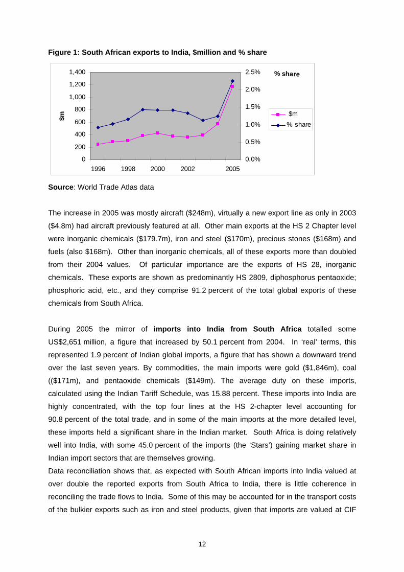
During 2005 South Africa exported merchandise worth $1,169 million to India, almost

doubling the 2004 figure of $574 million. This represented some 2.3 percent of South Africa’s

global exports during 2005, a figure that similarly doubled from the previous year (and

basically the ten year average). This is shown in Figure 1, with the big increase in 2005

obvious. Not shown is that India ranked as South Africa’s 14th most important export

destination; just behind Italy and Zimbabwe but ahead of France, Mozambique and Korea.

12

Figure 1: South African exports to India, $million and % share

0

200

400

600

800

1,000

1,200

1,400

1996 1998 2000 2002 2005

$m

0.0%

0.5%

1.0%

1.5%

2.0%

2.5% % share

$m% share

Source: World Trade Atlas data

The increase in 2005 was mostly aircraft ($248m), virtually a new export line as only in 2003

($4.8m) had aircraft previously featured at all. Other main exports at the HS 2 Chapter level

were inorganic chemicals ($179.7m), iron and steel ($170m), precious stones ($168m) and

fuels (also $168m). Other than inorganic chemicals, all of these exports more than doubled

from their 2004 values. Of particular importance are the exports of HS 28, inorganic

chemicals. These exports are shown as predominantly HS 2809, diphosphorus pentaoxide;

phosphoric acid, etc., and they comprise 91.2 percent of the total global exports of these

chemicals from South Africa.

During 2005 the mirror of imports into India from South Africa totalled some

US$2,651 million, a figure that increased by 50.1 percent from 2004. In ‘real’ terms, this

represented 1.9 percent of Indian global imports, a figure that has shown a downward trend

over the last seven years. By commodities, the main imports were gold ($1,846m), coal

(($171m), and pentaoxide chemicals ($149m). The average duty on these imports,

calculated using the Indian Tariff Schedule, was 15.88 percent. These imports into India are

highly concentrated, with the top four lines at the HS 2-chapter level accounting for

90.8 percent of the total trade, and in some of the main imports at the more detailed level,

these imports held a significant share in the Indian market. South Africa is doing relatively

well into India, with some 45.0 percent of the imports (the ‘Stars’) gaining market share in

Indian import sectors that are themselves growing.

Data reconciliation shows that, as expected with South African imports into India valued at

over double the reported exports from South Africa to India, there is little coherence in

reconciling the trade flows to India. Some of this may be accounted for in the transport costs

of the bulkier exports such as iron and steel products, given that imports are valued at CIF

13

and exports at FOB, while another large difference is that there are no reported exports of

gold from South Africa but this is the major import into India. In addition, the largest export

from South Africa (aircraft) is not reported in Indian import data. If we ignore this gold and

aircraft trade then the overall reconciliation is remarkably accurate.

(b) Indian imports into South Africa

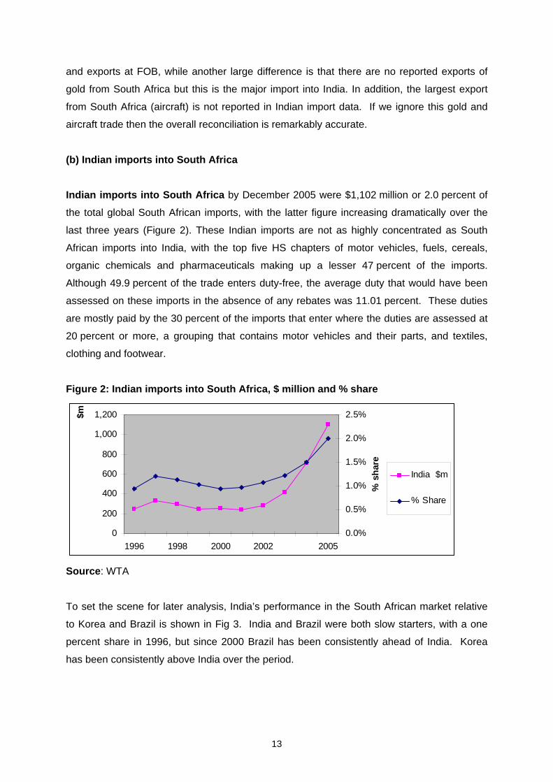
Indian imports into South Africa by December 2005 were $1,102 million or 2.0 percent of

the total global South African imports, with the latter figure increasing dramatically over the

last three years (Figure 2). These Indian imports are not as highly concentrated as South

African imports into India, with the top five HS chapters of motor vehicles, fuels, cereals,

organic chemicals and pharmaceuticals making up a lesser 47 percent of the imports.

Although 49.9 percent of the trade enters duty-free, the average duty that would have been

assessed on these imports in the absence of any rebates was 11.01 percent. These duties

are mostly paid by the 30 percent of the imports that enter where the duties are assessed at

20 percent or more, a grouping that contains motor vehicles and their parts, and textiles,

clothing and footwear.

Figure 2: Indian imports into South Africa, $ million and % share

0

200

400

600

800

1,000

1,200

1996 1998 2000 2002 2005

$m

0.0%

0.5%

1.0%

1.5%

2.0%

2.5%

% s

hare

India $m

% Share

Source: WTA

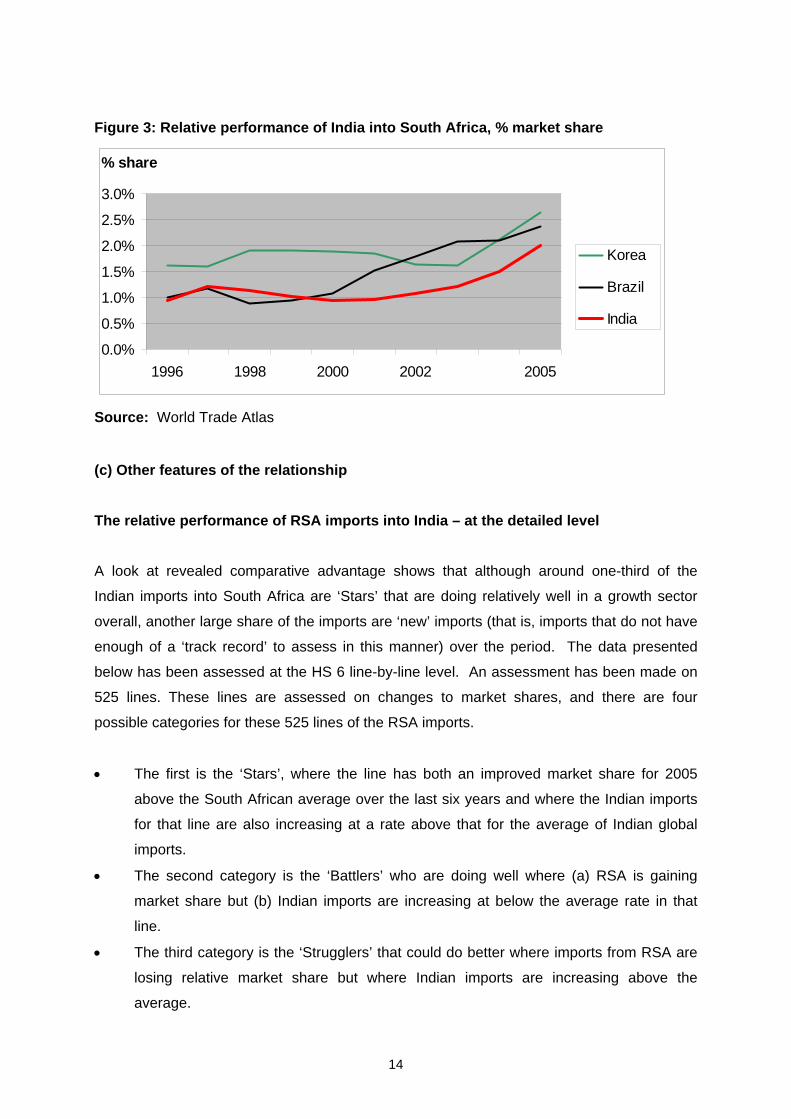
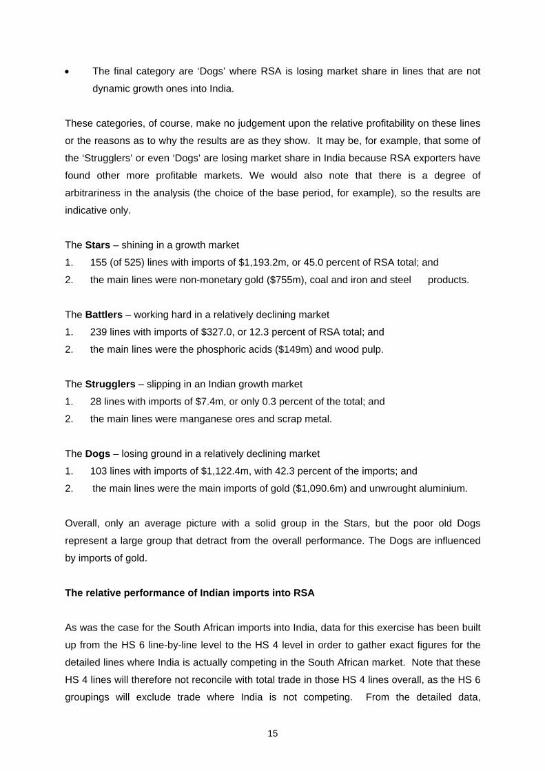
To set the scene for later analysis, India’s performance in the South African market relative

to Korea and Brazil is shown in Fig 3. India and Brazil were both slow starters, with a one

percent share in 1996, but since 2000 Brazil has been consistently ahead of India. Korea

has been consistently above India over the period.

14

Figure 3: Relative performance of India into South Africa, % market share

0.0%

0.5%

1.0%

1.5%

2.0%

2.5%

3.0%

1996 1998 2000 2002 2005

% share

Korea

Brazil

India


(c) Other features of the relationship The relative performance of RSA imports into India – at the detailed level

A look at revealed comparative advantage shows that although around one-third of the

Indian imports into South Africa are ‘Stars’ that are doing relatively well in a growth sector

overall, another large share of the imports are ‘new’ imports (that is, imports that do not have

enough of a ‘track record’ to assess in this manner) over the period. The data presented

below has been assessed at the HS 6 line-by-line level. An assessment has been made on

525 lines. These lines are assessed on changes to market shares, and there are four

possible categories for these 525 lines of the RSA imports.

• The first is the ‘Stars’, where the line has both an improved market share for 2005

above the South African average over the last six years and where the Indian imports

for that line are also increasing at a rate above that for the average of Indian global

imports.

• The second category is the ‘Battlers’ who are doing well where (a) RSA is gaining

market share but (b) Indian imports are increasing at below the average rate in that

line.

• The third category is the ‘Strugglers’ that could do better where imports from RSA are

losing relative market share but where Indian imports are increasing above the

average.

15

• The final category are ‘Dogs’ where RSA is losing market share in lines that are not

dynamic growth ones into India.

These categories, of course, make no judgement upon the relative profitability on these lines

or the reasons as to why the results are as they show. It may be, for example, that some of

the ‘Strugglers’ or even ‘Dogs’ are losing market share in India because RSA exporters have

found other more profitable markets. We would also note that there is a degree of

arbitrariness in the analysis (the choice of the base period, for example), so the results are

indicative only.

The Stars – shining in a growth market

1. 155 (of 525) lines with imports of $1,193.2m, or 45.0 percent of RSA total; and

2. the main lines were non-monetary gold ($755m), coal and iron and steel products.

The Battlers – working hard in a relatively declining market

1. 239 lines with imports of $327.0, or 12.3 percent of RSA total; and

2. the main lines were the phosphoric acids ($149m) and wood pulp.

The Strugglers – slipping in an Indian growth market

1. 28 lines with imports of $7.4m, or only 0.3 percent of the total; and

2. the main lines were manganese ores and scrap metal.

The Dogs – losing ground in a relatively declining market

1. 103 lines with imports of $1,122.4m, with 42.3 percent of the imports; and

2. the main lines were the main imports of gold ($1,090.6m) and unwrought aluminium.

Overall, only an average picture with a solid group in the Stars, but the poor old Dogs

represent a large group that detract from the overall performance. The Dogs are influenced

by imports of gold.

The relative performance of Indian imports into RSA

As was the case for the South African imports into India, data for this exercise has been built

up from the HS 6 line-by-line level to the HS 4 level in order to gather exact figures for the

detailed lines where India is actually competing in the South African market. Note that these

HS 4 lines will therefore not reconcile with total trade in those HS 4 lines overall, as the HS 6

groupings will exclude trade where India is not competing. From the detailed data,

16

information on the performance of individual lines can be assessed, and this can then been

aggregated into a ‘big picture’ profile. An assessment has been made on 577 aggregated HS

4 lines, with these lines containing some 99.8 percent of the total imports from India. The

cut-off point for these lines was where the import value from India during 2005 was US

$30,000 or more.

These lines are assessed on changes to market shares, and there are four possible

categories for these 577 lines, and a fifth where there were no imports from India in 1996.

This latter category could be because (a) India was not exporting that line globally, and/or (b)

South Africa was not importing in that line in 1996 (12 cases) because either the HS codes

have been changed or this is simply new trade. This category included imports of $248.2

million or 22.5 percent of the total. By definition the Indian market share had increased in all

cases, and in $219.9 million of this trade the particular global imports into South Africa have

increased above the average. This suggests that India is also doing well in these imports.

The Stars – shining in a growth market

* 95 (of 406) lines with imports of $393.0 million, or 35.7% of Indian total imports;

The Battlers – working hard in a relatively declining market

* 200 lines with imports of $354.0 million, or 32.2% of the Indian total;

The Strugglers – slipping in a South African growth market

* 61 lines with imports of $71.0 million, or 6.4% of the total;

The Dogs – losing ground in a relatively declining South African market

* 50 lines with imports of $24.7million, or 2.2% of the imports.

Note that a further $248.2 million (22.5%) has been classified as ‘new’ trade, where there

were no recorded imports from India in the base year. These could also be classified as

either ‘stars’ or ‘battlers’, depending upon the relative growth of South African global imports

in that sector.

For the ‘big ticket’ import lines, fuel ($123m) is ‘new’, three lines of motor vehicles ($160m)

are ‘stars’, as is a pharmaceutical line (48.8m), while rice ($73,9m) and heavy vehicles

($27.8m) are both ‘battlers’. If we modify the questions asked above and instead ask the

question, ‘Is India gaining market share in the South African imports of this particular line?’

the answer is very different. For some 88 percent of the individual imports as assessed at

17

the HS line level into South Africa, India has actually gained market share over its

competitors. That is a good performance, but of course it includes most of the ‘new’ trade as

defined.

Other analytical tools from the kit-bag

‘Trade chilling’ suggests that there are few additional areas where South Africa could export

to India and where an FTA could help. Analysis at the detailed level shows that where South

Africa is active in the Indian market, the Republic is competing strongly, as those lines where

South Africa has a market share of at least one percent account for 98.6 percent of the South

African imports but only 17.1 percent of the Indian global imports. Thus, South Africa is doing

very well given its global export mix and India’s global import profile.

More specifically, the ‘trade chilling’ analysis was undertaken on a combination of (a) the 149

HS 4 tariff lines where global agricultural imports into India were at least $100,000 during

2005 to represent the demand side, and (b) these were then compared with the respective

HS 4 tariff lines exported to global markets from South Africa during 2005 to represent the

supply side. From there, five categories were examined. These are7:

1) Where South African imports held at least a 1 percent market share in India;

2) Where at least 1 percent of South African exports went to India;

3) Where South Africa records positive exports to India in 2005 but India does not record

positive imports from South Africa;

4) Where positive imports are recorded into India from South Africa but no exports from

South Africa are reported;

5) Where there is at least $1 million exported from South Africa globally but no reported

imports of this trade into India from South Africa.

Analysis of the data showed that there were only two classifications of interest, 1 and 5, as

almost all the current trade was in category 1 and there was effectively no trade in categories

2, 3 and 4. The results therefore are:

• South Africa has at least a 1 percent share in all the major import lines into India.

There are 13 HS 4 lines, and these imports accounted for 94.8 percent of South

7 Note that, in a direct comparison with China, India does not administer any Tariff Rate Quotas

(TRQs) on agricultural products.

18

African agricultural exports to India and 95.8 percent of the total imports from South

Africa into India during 2005. This also highlights that there is a reasonable degree of

trade reconciliation between South African exports to India and Indian imports from

South Africa.

• Where India imports these goods and South Africa exported at least rand 1 million globally during 2005 but the twain did not meet – this is potentially the

important category for examination, as it clearly shows there are both supply and

demand factors that are not, for whatever reason, meeting. However, a careful

analysis shows that there are virtually no potential trade items in this category.

Tobacco and tobacco products are one reasonable possibility, and at a stretch maybe

sunflower oil. The only other possible products are milk powders, soya flour and corn

maize, although South African global exports of these products are all under

$10 million and Indian imports are even lower at below $1.4 million in each case.

In looking to the future and visualising a FTA between India and SACU/South Africa there

appear to be some sectors where South Africa may gain, but this seems likely to be based

entirely upon tariff preferences in a few selected lines only (with sugar the main one).

Finally, an analysis of the so-called intra-Industry trade between South Africa and India

shows that, as expected between two developing countries, these index values are low at the

5.3 (out of a 100) level. This index compares trade between partners in like products, and is

a feature of trade between developed countries. However, the more interesting feature is that

these index values are steadily increasing from very low levels over the last ten years,

suggesting an increasing sophistication in the trading relationship.

The South African/Brazilian trading relationship

(a) South African exports/Brazilian imports

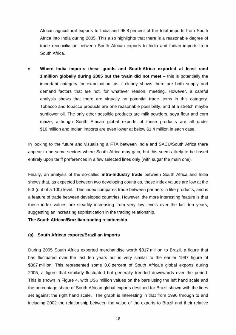
During 2005 South Africa exported merchandise worth $317 million to Brazil, a figure that

has fluctuated over the last ten years but is very similar to the earlier 1997 figure of

$307 million. This represented some 0.6 percent of South Africa’s global exports during

2005, a figure that similarly fluctuated but generally trended downwards over the period.

This is shown in Figure 4, with US$ million values on the bars using the left hand scale and

the percentage share of South African global exports destined for Brazil shown with the lines

set against the right hand scale. The graph is interesting in that from 1996 through to and

including 2002 the relationship between the value of the exports to Brazil and their relative

19

share of South African global exports stayed almost exactly the same. From that 2003 this

close relationship was broken as the values grew faster than the percentage, highlighting just

how fast South African global exports were increasing.

Figure 4: South African exports to Brazil, $ million and export share

0

50

100

150

200

250

300

350

1996 1998 2000 2002 2005

$m

0.0%

0.2%

0.4%

0.6%

0.8%

1.0%

1.2%

% s

hare $m

% tot


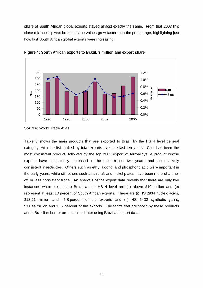
Table 3 shows the main products that are exported to Brazil by the HS 4 level general

category, with the list ranked by total exports over the last ten years. Coal has been the

most consistent product, followed by the top 2005 export of ferroalloys, a product whose

exports have consistently increased in the most recent two years, and the relatively

consistent insecticides. Others such as ethyl alcohol and phosphoric acid were important in

the early years, while still others such as aircraft and nickel plates have been more of a one-

off or less consistent trade. An analysis of the export data reveals that there are only two

instances where exports to Brazil at the HS 4 level are (a) above $10 million and (b)

represent at least 10 percent of South African exports. These are (i) HS 2934 nucleic acids,

$13.21 million and 45.8 percent of the exports and (ii) HS 5402 synthetic yarns,

$11.44 million and 13.2 percent of the exports. The tariffs that are faced by these products

at the Brazilian border are examined later using Brazilian import data.

20

Table 3: South African exports to Brazil, $ million Description/Year 1996 1997 1998 1999 2000 2001 2002 2003 2004 2005

Total 272 307 197 155 200 275 171 177 242 317

coal 35.7 49.7 51.5 37.1 29.8 34.8 28.4 22.5 26.9 29.1

ferroalloys 9.5 9.1 6.7 5.2 8.9 12.7 12.5 25.3 50.3 50.6

insecticides etc 13.2 20.2 12.5 12.9 23.6 33.9 21.3 19.9 11.3 7.9

ethyl alcohol 73.7 60.0 0.0 1.2 5.7 0.2 0.0 0.0 0.0 0.0

aluminium plates 0.0 0.0 0.4 3.8 12.5 16.7 8.7 15.3 13.7 17.3

phosphoric acid 22.8 27.5 17.2 5.0 3.3 5.0 0.7 0.0 0.0 0.0

aircraft 0.0 0.0 0.3 1.4 0.0 66.1 4.7 0.0 0.0 0.4

synthetic yarn 3.3 9.7 5.3 4.6 7.2 6.5 6.0 6.4 8.4 11.4

nickel plates 0.0 0.0 8.1 14.2 17.7 6.9 6.2 0.0 0.0 1.5

ketones 4.0 1.8 1.0 2.9 3.7 2.3 3.2 6.0 7.7 10.5

engine parts 0.0 0.1 0.3 0.1 1.1 3.0 3.0 13.5 10.4 10.6

stainless steel 5.3 6.5 4.2 2.2 4.3 4.9 5.9 2.1 1.6 0.5

hydrocarbons 0.4 1.0 0.8 0.9 2.2 3.9 2.9 3.5 6.2 12.4

nucleic acid 2.9 3.0 0.0 0.0 0.0 0.0 0.0 0.0 5.5 13.2


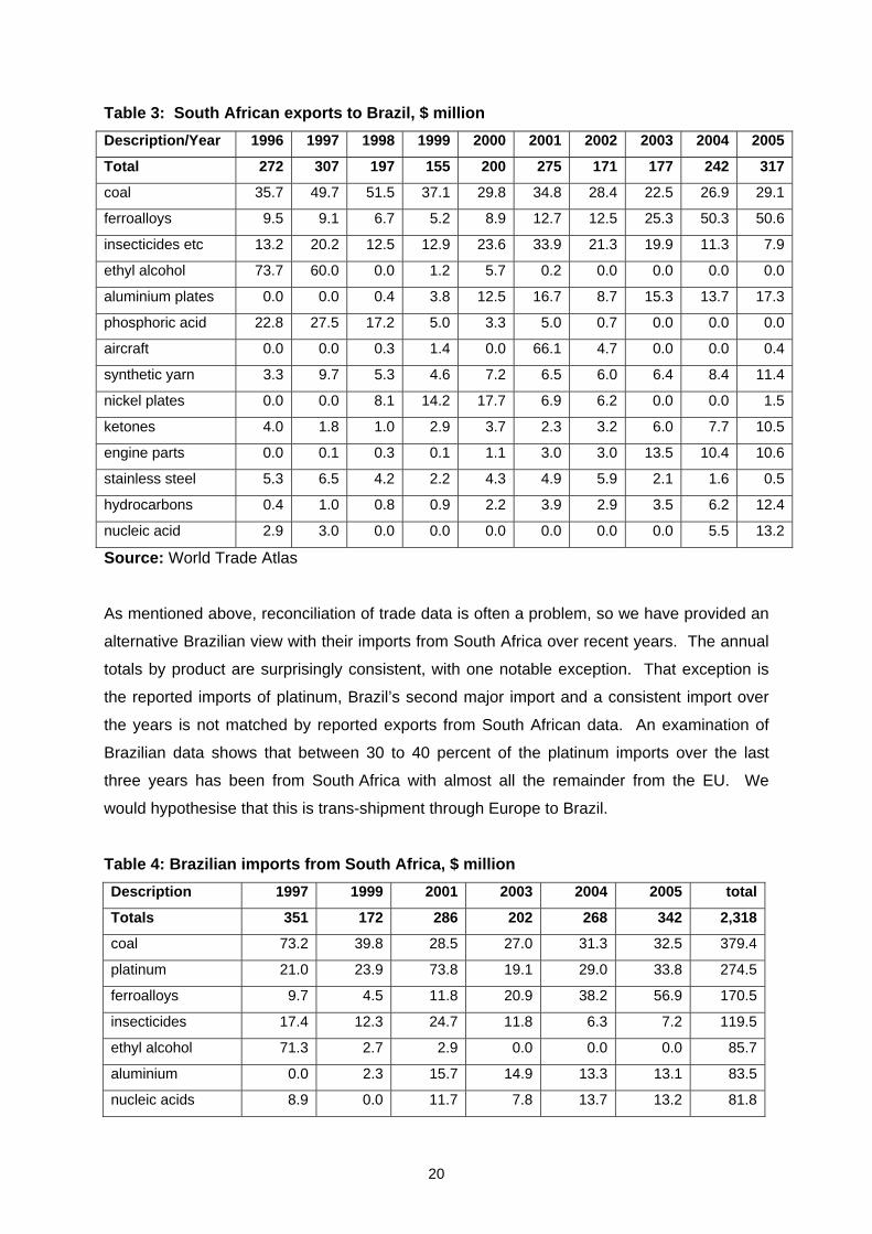
As mentioned above, reconciliation of trade data is often a problem, so we have provided an

alternative Brazilian view with their imports from South Africa over recent years. The annual

totals by product are surprisingly consistent, with one notable exception. That exception is

the reported imports of platinum, Brazil’s second major import and a consistent import over

the years is not matched by reported exports from South African data. An examination of

Brazilian data shows that between 30 to 40 percent of the platinum imports over the last

three years has been from South Africa with almost all the remainder from the EU. We

would hypothesise that this is trans-shipment through Europe to Brazil.

Table 4: Brazilian imports from South Africa, $ million Description 1997 1999 2001 2003 2004 2005 total

Totals 351 172 286 202 268 342 2,318

coal 73.2 39.8 28.5 27.0 31.3 32.5 379.4

platinum 21.0 23.9 73.8 19.1 29.0 33.8 274.5

ferroalloys 9.7 4.5 11.8 20.9 38.2 56.9 170.5

insecticides 17.4 12.3 24.7 11.8 6.3 7.2 119.5

ethyl alcohol 71.3 2.7 2.9 0.0 0.0 0.0 85.7

aluminium 0.0 2.3 15.7 14.9 13.3 13.1 83.5

nucleic acids 8.9 0.0 11.7 7.8 13.7 13.2 81.8

21

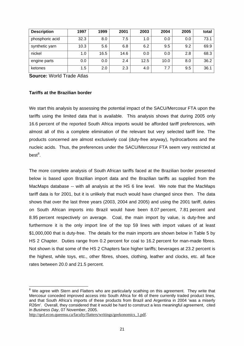
Description 1997 1999 2001 2003 2004 2005 total

phosphoric acid 32.3 8.0 7.5 1.0 0.0 0.0 73.1

synthetic yarn 10.3 5.6 6.8 6.2 9.5 9.2 69.9

nickel 1.0 16.5 14.6 0.0 0.0 2.8 68.3

engine parts 0.0 0.0 2.4 12.5 10.0 8.0 36.2

ketones 1.5 2.0 2.3 4.0 7.7 9.5 36.1


Tariffs at the Brazilian border

We start this analysis by assessing the potential impact of the SACU/Mercosur FTA upon the

tariffs using the limited data that is available. This analysis shows that during 2005 only

16.6 percent of the reported South Africa imports would be afforded tariff preferences, with

almost all of this a complete elimination of the relevant but very selected tariff line. The

products concerned are almost exclusively coal (duty-free anyway), hydrocarbons and the

nucleic acids. Thus, the preferences under the SACU/Mercosur FTA seem very restricted at

best8.

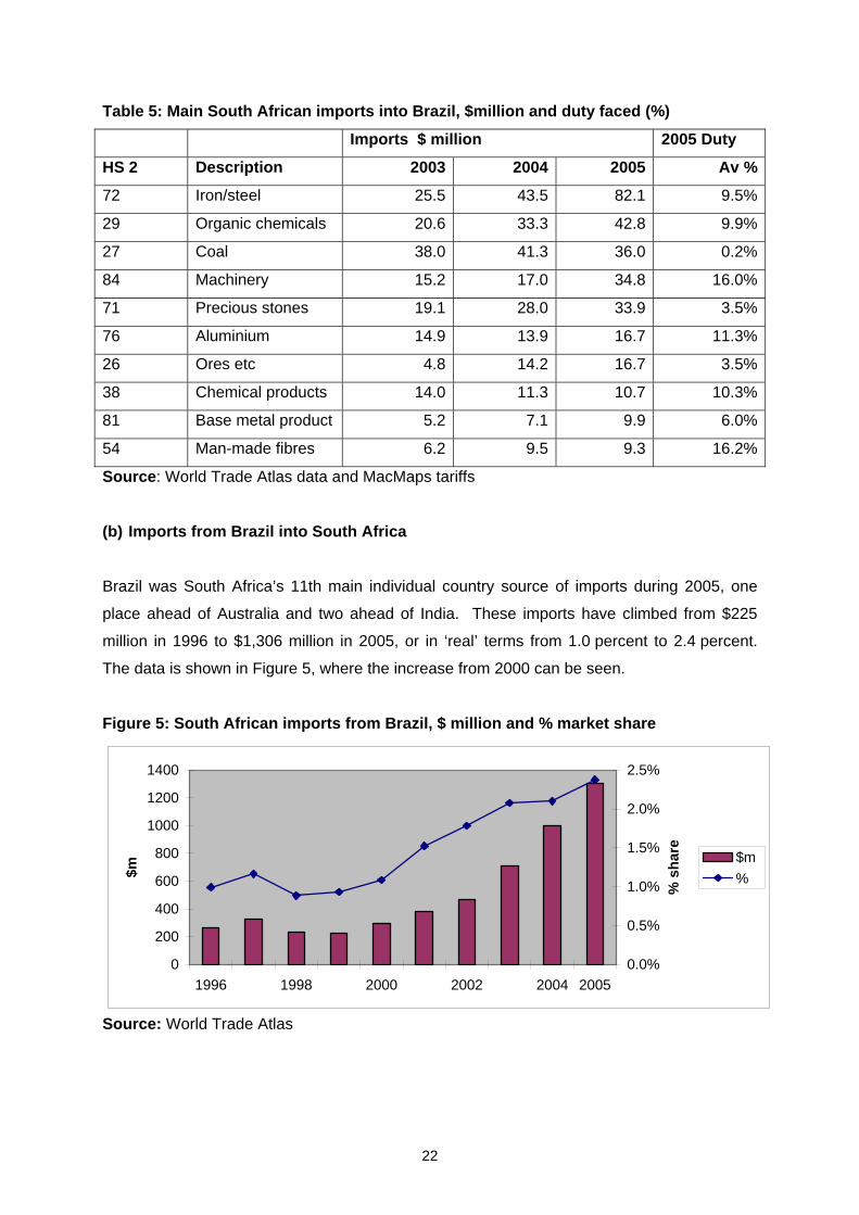
The more complete analysis of South African tariffs faced at the Brazilian border presented

below is based upon Brazilian import data and the Brazilian tariffs as supplied from the

MacMaps database -- with all analysis at the HS 6 line level. We note that the MacMaps

tariff data is for 2001, but it is unlikely that much would have changed since then. The data

shows that over the last three years (2003, 2004 and 2005) and using the 2001 tariff, duties

on South African imports into Brazil would have been 8.07 percent, 7.81 percent and

8.95 percent respectively on average. Coal, the main import by value, is duty-free and

furthermore it is the only import line of the top 59 lines with import values of at least

$1,000,000 that is duty-free. The details for the main imports are shown below in Table 5 by

HS 2 Chapter. Duties range from 0.2 percent for coal to 16.2 percent for man-made fibres.

Not shown is that some of the HS 2 Chapters face higher tariffs; beverages at 23.2 percent is

the highest, while toys, etc., other fibres, shoes, clothing, leather and clocks, etc. all face

rates between 20.0 and 21.5 percent.

8 We agree with Stern and Flatters who are particularly scathing on this agreement. They write that Mercosur conceded improved access into South Africa for 46 of there currently traded product lines, and that South Africa’s imports of these products from Brazil and Argentina in 2004 ‘was a miserly R26m’. Overall, they considered that it would be hard to construct a less meaningful agreement, cited in Business Day, 07 November, 2005. http://qed.econ.queensu.ca/faculty/flatters/writings/geekonomics_1.pdf..

22

Table 5: Main South African imports into Brazil, $million and duty faced (%)

Imports $ million 2005 Duty

HS 2 Description 2003 2004 2005 Av %

72 Iron/steel 25.5 43.5 82.1 9.5%

29 Organic chemicals 20.6 33.3 42.8 9.9%

27 Coal 38.0 41.3 36.0 0.2%

84 Machinery 15.2 17.0 34.8 16.0%

71 Precious stones 19.1 28.0 33.9 3.5%

76 Aluminium 14.9 13.9 16.7 11.3%

26 Ores etc 4.8 14.2 16.7 3.5%

38 Chemical products 14.0 11.3 10.7 10.3%

81 Base metal product 5.2 7.1 9.9 6.0%

54 Man-made fibres 6.2 9.5 9.3 16.2%

Source: World Trade Atlas data and MacMaps tariffs

(b) Imports from Brazil into South Africa

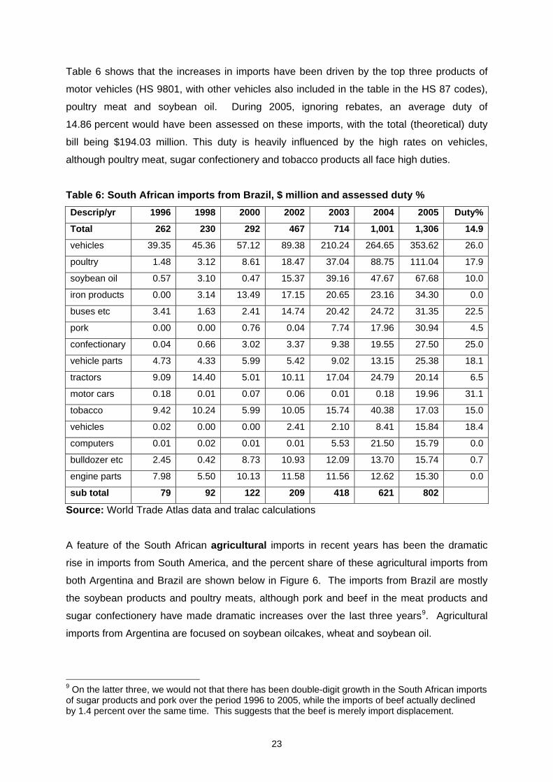
Brazil was South Africa’s 11th main individual country source of imports during 2005, one

place ahead of Australia and two ahead of India. These imports have climbed from $225

million in 1996 to $1,306 million in 2005, or in ‘real’ terms from 1.0 percent to 2.4 percent.

The data is shown in Figure 5, where the increase from 2000 can be seen.

Figure 5: South African imports from Brazil, $ million and % market share

0

200

400

600

800

1000

1200

1400

1996 1998 2000 2002 2004 2005

$m

0.0%

0.5%

1.0%

1.5%

2.0%

2.5%

% s

hare $m

%


23

Table 6 shows that the increases in imports have been driven by the top three products of

motor vehicles (HS 9801, with other vehicles also included in the table in the HS 87 codes),

poultry meat and soybean oil. During 2005, ignoring rebates, an average duty of

14.86 percent would have been assessed on these imports, with the total (theoretical) duty

bill being $194.03 million. This duty is heavily influenced by the high rates on vehicles,

although poultry meat, sugar confectionery and tobacco products all face high duties.

Table 6: South African imports from Brazil, $ million and assessed duty % Descrip/yr 1996 1998 2000 2002 2003 2004 2005 Duty%

Total 262 230 292 467 714 1,001 1,306 14.9

vehicles 39.35 45.36 57.12 89.38 210.24 264.65 353.62 26.0

poultry 1.48 3.12 8.61 18.47 37.04 88.75 111.04 17.9

soybean oil 0.57 3.10 0.47 15.37 39.16 47.67 67.68 10.0

iron products 0.00 3.14 13.49 17.15 20.65 23.16 34.30 0.0

buses etc 3.41 1.63 2.41 14.74 20.42 24.72 31.35 22.5

pork 0.00 0.00 0.76 0.04 7.74 17.96 30.94 4.5

confectionary 0.04 0.66 3.02 3.37 9.38 19.55 27.50 25.0

vehicle parts 4.73 4.33 5.99 5.42 9.02 13.15 25.38 18.1

tractors 9.09 14.40 5.01 10.11 17.04 24.79 20.14 6.5

motor cars 0.18 0.01 0.07 0.06 0.01 0.18 19.96 31.1

tobacco 9.42 10.24 5.99 10.05 15.74 40.38 17.03 15.0

vehicles 0.02 0.00 0.00 2.41 2.10 8.41 15.84 18.4

computers 0.01 0.02 0.01 0.01 5.53 21.50 15.79 0.0

bulldozer etc 2.45 0.42 8.73 10.93 12.09 13.70 15.74 0.7

engine parts 7.98 5.50 10.13 11.58 11.56 12.62 15.30 0.0

sub total 79 92 122 209 418 621 802

Source: World Trade Atlas data and tralac calculations

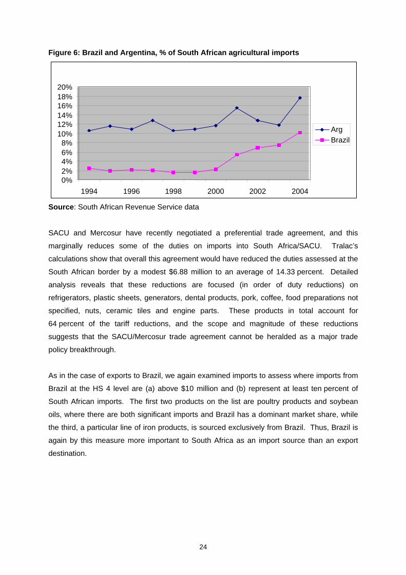
A feature of the South African agricultural imports in recent years has been the dramatic

rise in imports from South America, and the percent share of these agricultural imports from

both Argentina and Brazil are shown below in Figure 6. The imports from Brazil are mostly

the soybean products and poultry meats, although pork and beef in the meat products and

sugar confectionery have made dramatic increases over the last three years9. Agricultural

imports from Argentina are focused on soybean oilcakes, wheat and soybean oil.

9 On the latter three, we would not that there has been double-digit growth in the South African imports of sugar products and pork over the period 1996 to 2005, while the imports of beef actually declined by 1.4 percent over the same time. This suggests that the beef is merely import displacement.

24

Figure 6: Brazil and Argentina, % of South African agricultural imports

Source: South African Revenue Service data

SACU and Mercosur have recently negotiated a preferential trade agreement, and this

marginally reduces some of the duties on imports into South Africa/SACU. Tralac’s

calculations show that overall this agreement would have reduced the duties assessed at the

South African border by a modest $6.88 million to an average of 14.33 percent. Detailed

analysis reveals that these reductions are focused (in order of duty reductions) on

refrigerators, plastic sheets, generators, dental products, pork, coffee, food preparations not

specified, nuts, ceramic tiles and engine parts. These products in total account for

64 percent of the tariff reductions, and the scope and magnitude of these reductions

suggests that the SACU/Mercosur trade agreement cannot be heralded as a major trade

policy breakthrough.

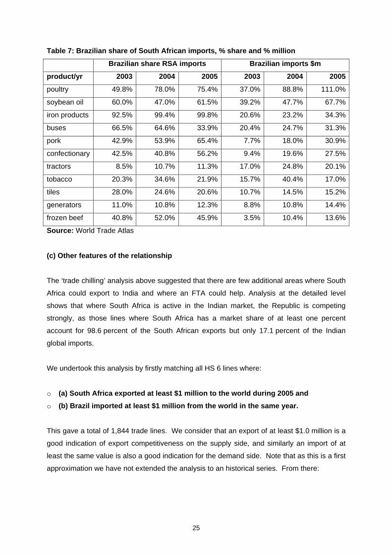
As in the case of exports to Brazil, we again examined imports to assess where imports from

Brazil at the HS 4 level are (a) above $10 million and (b) represent at least ten percent of

South African imports. The first two products on the list are poultry products and soybean

oils, where there are both significant imports and Brazil has a dominant market share, while

the third, a particular line of iron products, is sourced exclusively from Brazil. Thus, Brazil is

again by this measure more important to South Africa as an import source than an export

destination.

0% 2% 4% 6% 8%

10% 12% 14% 16% 18% 20%

1994 1996 1998 2000 2002 2004

ArgBrazil

25

Table 7: Brazilian share of South African imports, % share and % million

Brazilian share RSA imports Brazilian imports $m

product/yr 2003 2004 2005 2003 2004 2005

poultry 49.8% 78.0% 75.4% 37.0% 88.8% 111.0%

soybean oil 60.0% 47.0% 61.5% 39.2% 47.7% 67.7%

iron products 92.5% 99.4% 99.8% 20.6% 23.2% 34.3%

buses 66.5% 64.6% 33.9% 20.4% 24.7% 31.3%

pork 42.9% 53.9% 65.4% 7.7% 18.0% 30.9%

confectionary 42.5% 40.8% 56.2% 9.4% 19.6% 27.5%

tractors 8.5% 10.7% 11.3% 17.0% 24.8% 20.1%

tobacco 20.3% 34.6% 21.9% 15.7% 40.4% 17.0%

tiles 28.0% 24.6% 20.6% 10.7% 14.5% 15.2%

generators 11.0% 10.8% 12.3% 8.8% 10.8% 14.4%

frozen beef 40.8% 52.0% 45.9% 3.5% 10.4% 13.6%


(c) Other features of the relationship

The ‘trade chilling’ analysis above suggested that there are few additional areas where South

Africa could export to India and where an FTA could help. Analysis at the detailed level

shows that where South Africa is active in the Indian market, the Republic is competing

strongly, as those lines where South Africa has a market share of at least one percent

account for 98.6 percent of the South African exports but only 17.1 percent of the Indian

global imports.

We undertook this analysis by firstly matching all HS 6 lines where:

o (a) South Africa exported at least $1 million to the world during 2005 and o (b) Brazil imported at least $1 million from the world in the same year.

This gave a total of 1,844 trade lines. We consider that an export of at least $1.0 million is a

good indication of export competitiveness on the supply side, and similarly an import of at

least the same value is also a good indication for the demand side. Note that as this is a first

approximation we have not extended the analysis to an historical series. From there:

26

1. There were 922 lines where at least one percent of these South African exports went

to Brazil. This represented (a) some 83 percent of the South African exports to Brazil

and a (b) lesser 72 percent of the Brazilian imports from South Africa.

2. There were 897 lines where South Africa held at least a one percent share in the

Brazilian market. This represented (a) some 83 percent of the South African exports to

Brazil and (b) a greater 89 percent of the South African imports into Brazil. Note that

this category will include, as discussed above, Brazilian imports of platinum that are

not reported as South African exports.

3. Combining (1) and (2) gives a total of 960 lines (there are many duplicates where both

(a) and (b) hold), for (a) 92.6 percent of the South African exports and (b) 90 percent of

the Brazilian imports from South Africa. Thus, the overall pattern is that South Africa is

competing strongly in the Brazilian market.

4. Where a positive import value is reported into Brazil from South Africa, but (i)

where this trade that may or may not be reported as exports from South Africa and (ii)

where the South African market share is less than one percent of the Brazilian market

and less than one percent of the South African exports are destined for Brazil. This is a

small (only 1.7% of the imports and a lesser 1.2% of the exports) and rather eclectic

mix of exclusively non-agricultural products where South Africa could possibly be doing

better.

5. Where a positive export value is reported from South Africa to Brazil, but where

this trade that may or may not be reported as imports from South Africa and where

again both market shares are less than one percent (i.e. very small values in any

case). This represents only 0.83% of the exports, and these products are a rather

eclectic mix of exclusively non-agricultural products where South Africa could possibly

be doing better.

The final category is where (a) Brazil imports these goods from other global sources to the

value of at least $5 million and (b) South Africa similarly exported at least $5 million globally

during 2005 but (c) the twain did not meet. This is potentially the important category for examination, as it clearly shows there are both supply and demand factors that are not, for

whatever reason, meeting. This set constituted some 23 percent of South African global

exports and a lesser 13 percent of Brazilian imports. This is a significant finding, as it

indicates that there are favourable conditions on both the supply (South African exports) and

demand (Brazilian imports) sides that are not being matched by commercial transactions.

There are of course multiple reasons why this may be the case, but it does point to clear

opportunities on the South African side at least (as we have not undertaken the similar

analysis for Brazilian exports to South Africa). There are a large number (142 HS 6 lines) of

27

again all manufacturing products covered here that represent a very wide range of broad

categories. Many of these have what could be termed ‘asymmetrical trade’ in that either

South African global exports are very large and imports small or conversely Brazilian imports

are very large and South African global exports are minor, but there are some areas such as

motor vehicles in particular and chemicals where both countries are big traders but not with

each other.

The Indian/Brazilian trading relationship

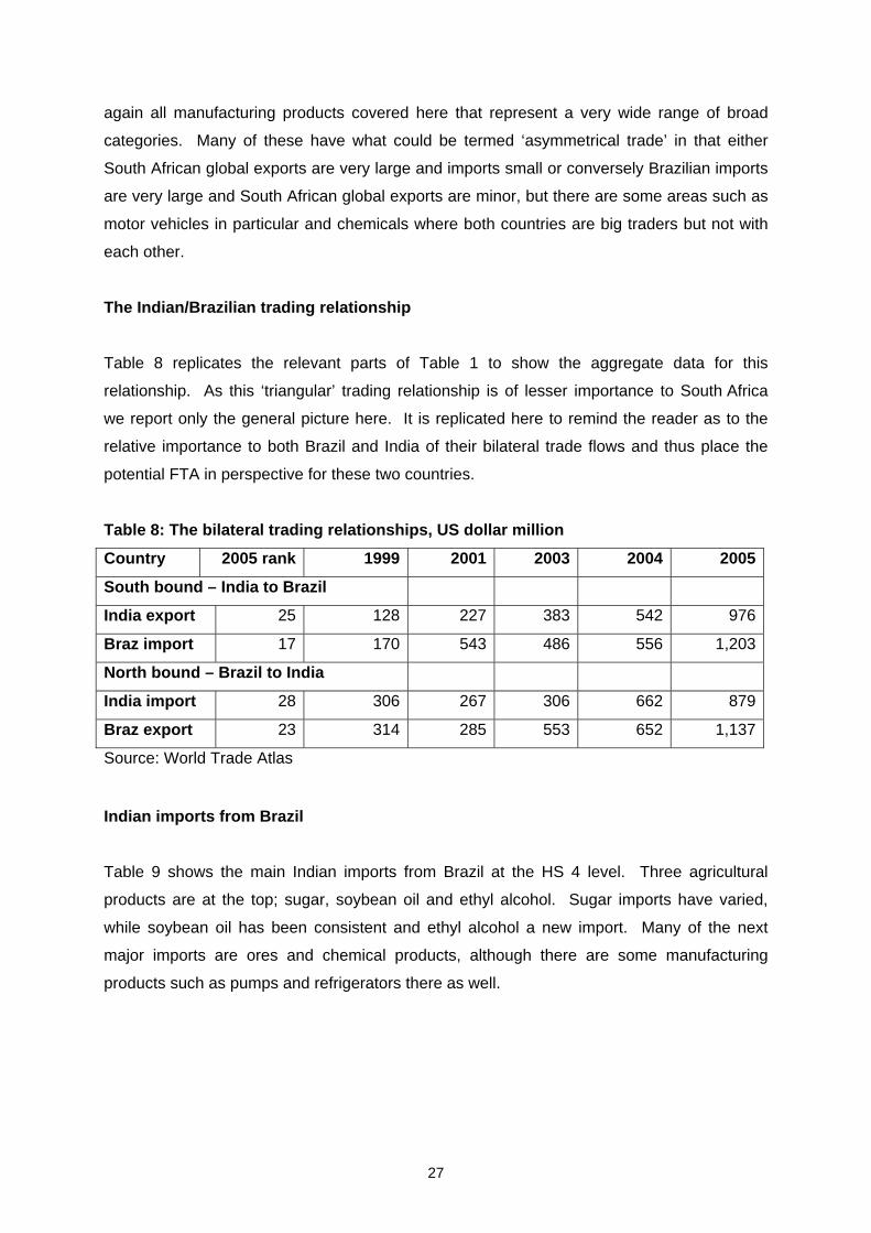
Table 8 replicates the relevant parts of Table 1 to show the aggregate data for this

relationship. As this ‘triangular’ trading relationship is of lesser importance to South Africa

we report only the general picture here. It is replicated here to remind the reader as to the

relative importance to both Brazil and India of their bilateral trade flows and thus place the

potential FTA in perspective for these two countries.

Table 8: The bilateral trading relationships, US dollar million

Country 2005 rank 1999 2001 2003 2004 2005

South bound – India to Brazil

India export 25 128 227 383 542 976

Braz import 17 170 543 486 556 1,203

North bound – Brazil to India

India import 28 306 267 306 662 879

Braz export 23 314 285 553 652 1,137


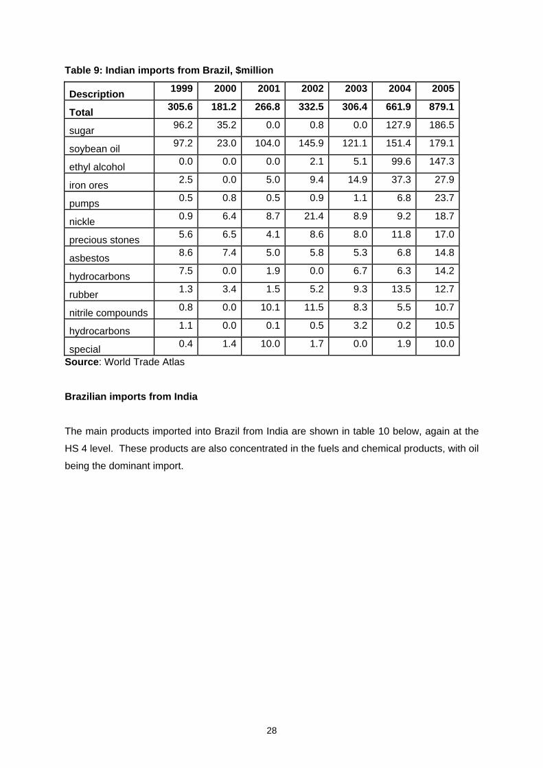
Indian imports from Brazil

Table 9 shows the main Indian imports from Brazil at the HS 4 level. Three agricultural

products are at the top; sugar, soybean oil and ethyl alcohol. Sugar imports have varied,

while soybean oil has been consistent and ethyl alcohol a new import. Many of the next

major imports are ores and chemical products, although there are some manufacturing

products such as pumps and refrigerators there as well.

28

Table 9: Indian imports from Brazil, $million

Description 1999 2000 2001 2002 2003 2004 2005

Total 305.6 181.2 266.8 332.5 306.4 661.9 879.1

sugar 96.2 35.2 0.0 0.8 0.0 127.9 186.5

soybean oil 97.2 23.0 104.0 145.9 121.1 151.4 179.1

ethyl alcohol 0.0 0.0 0.0 2.1 5.1 99.6 147.3

iron ores 2.5 0.0 5.0 9.4 14.9 37.3 27.9

pumps 0.5 0.8 0.5 0.9 1.1 6.8 23.7

nickle 0.9 6.4 8.7 21.4 8.9 9.2 18.7

precious stones 5.6 6.5 4.1 8.6 8.0 11.8 17.0

asbestos 8.6 7.4 5.0 5.8 5.3 6.8 14.8

hydrocarbons 7.5 0.0 1.9 0.0 6.7 6.3 14.2

rubber 1.3 3.4 1.5 5.2 9.3 13.5 12.7

nitrile compounds 0.8 0.0 10.1 11.5 8.3 5.5 10.7

hydrocarbons 1.1 0.0 0.1 0.5 3.2 0.2 10.5

special 0.4 1.4 10.0 1.7 0.0 1.9 10.0


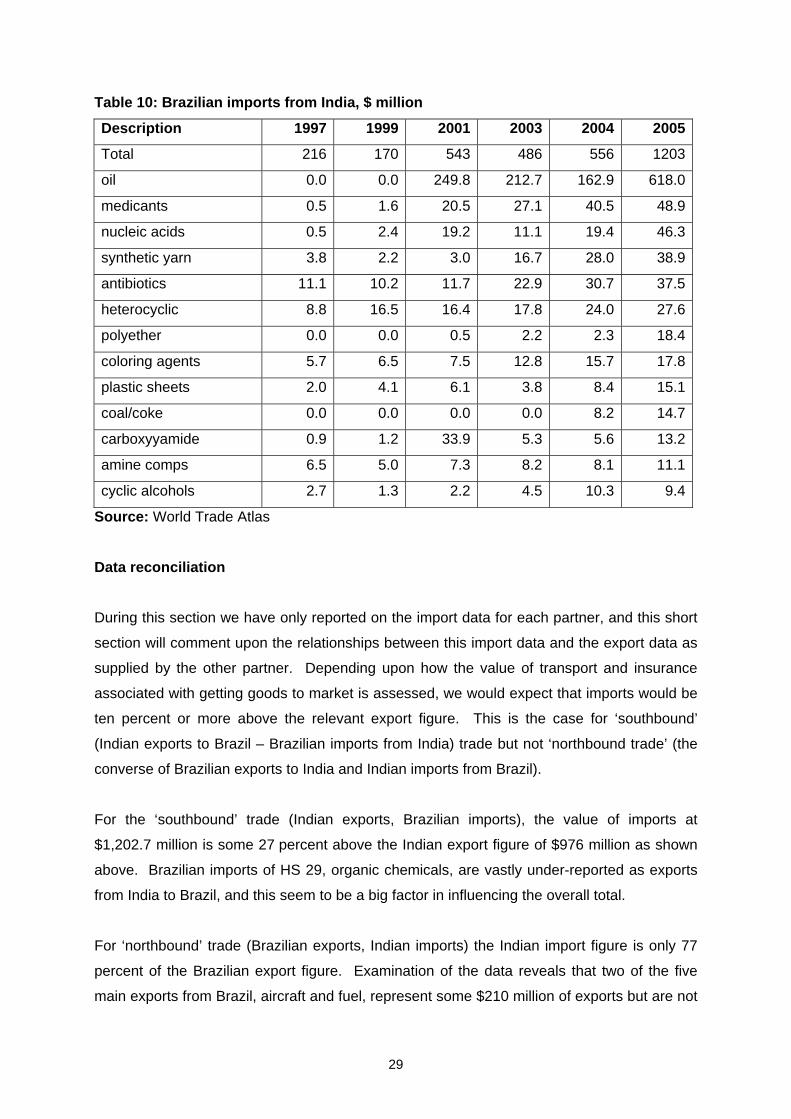
Brazilian imports from India

The main products imported into Brazil from India are shown in table 10 below, again at the

HS 4 level. These products are also concentrated in the fuels and chemical products, with oil

being the dominant import.

29

Table 10: Brazilian imports from India, $ million

Description 1997 1999 2001 2003 2004 2005

Total 216 170 543 486 556 1203

oil 0.0 0.0 249.8 212.7 162.9 618.0

medicants 0.5 1.6 20.5 27.1 40.5 48.9

nucleic acids 0.5 2.4 19.2 11.1 19.4 46.3

synthetic yarn 3.8 2.2 3.0 16.7 28.0 38.9

antibiotics 11.1 10.2 11.7 22.9 30.7 37.5

heterocyclic 8.8 16.5 16.4 17.8 24.0 27.6

polyether 0.0 0.0 0.5 2.2 2.3 18.4

coloring agents 5.7 6.5 7.5 12.8 15.7 17.8

plastic sheets 2.0 4.1 6.1 3.8 8.4 15.1

coal/coke 0.0 0.0 0.0 0.0 8.2 14.7

carboxyyamide 0.9 1.2 33.9 5.3 5.6 13.2

amine comps 6.5 5.0 7.3 8.2 8.1 11.1

cyclic alcohols 2.7 1.3 2.2 4.5 10.3 9.4


Data reconciliation

During this section we have only reported on the import data for each partner, and this short

section will comment upon the relationships between this import data and the export data as

supplied by the other partner. Depending upon how the value of transport and insurance

associated with getting goods to market is assessed, we would expect that imports would be

ten percent or more above the relevant export figure. This is the case for ‘southbound’

(Indian exports to Brazil – Brazilian imports from India) trade but not ‘northbound trade’ (the

converse of Brazilian exports to India and Indian imports from Brazil).

For the ‘southbound’ trade (Indian exports, Brazilian imports), the value of imports at

$1,202.7 million is some 27 percent above the Indian export figure of $976 million as shown

above. Brazilian imports of HS 29, organic chemicals, are vastly under-reported as exports

from India to Brazil, and this seem to be a big factor in influencing the overall total.

For ‘northbound’ trade (Brazilian exports, Indian imports) the Indian import figure is only 77

percent of the Brazilian export figure. Examination of the data reveals that two of the five

main exports from Brazil, aircraft and fuel, represent some $210 million of exports but are not

30

reported as imports into India. This makes a big difference in rectifying the overall data. We

would note that aircraft are not an infrequent cause of data problems, as sometimes

confusion may exist between one country classifying the transaction as an exports and

another as a lease, with the latter not included in merchandise trade data10. Of the other

main exports, sugar is under-reported into India (or over-reported from Brazil?) while

soybean oils are also inclined that way but the ethyl alcohol trade looks about right. We have

not examined quantity data.

Overall conclusions

All three partners share important and somewhat equal trading relationships.

Firstly, South Africa’s major exports to the world are concentrated in minerals and related

products. The major global exports by the general HS 2 Chapter has been precious stones

etc (platinum, gold and diamonds), followed by iron and steel products, mineral fuels and

motor vehicles, and these four products made up 55.6 percent of the total exports during

2005. The main export to India during 2005 was the one-off aircraft, followed by inorganic

chemicals, iron and steel products and again precious stones. These top four accounted for

65.5 percent of the total South African exports to India, and in addition we would note that

Indian import data shows the precious stones, metals and minerals, etc., may be under-

reported in the export data. Our analysis suggests that these exports face an average tariff

of some 15.88 percent using Indian import data. The main exports to Brazil were iron and

steel, organic chemicals, general machinery and mineral fuels, with these four comprising

63.3 percent of the total. Again, tralac analysis suggests these products faced an average

duty of 8.95 percent during 2005, and that the proposed SACU/Mercosur FTA would make

little difference to this rate.

Secondly, India’s main exports to the world are precious metals and stones, mineral fuels,

clothing and organic chemicals, with these four making up a lesser 36.3 percent of the total.

There is a direct linkage between India’s exports of precious jewellery and South Africa’s

base metal exports, as India has become the main processing and trading centre globally for

these often South Africa-sourced raw materials. Exports to South Africa were concentrated

in mineral fuels, vehicles, cereals and iron and steel products, with these exports making up

52.9 percent of the total. Indian exports to Brazil were mineral fuels (49.6% of the total),

10 We understand that this is probably what happened. In 2005, SAA leased an almost brand-new Airbus to an Indian airline.

31

organic chemicals, pharmaceuticals and miscellaneous chemical products, with the top four

comprising 71.3 percent of the total.

Finally, Brazilian global exports are even more diversified than India’s, with the top four of

vehicles, machinery, iron and steel and ores, etc. comprising 32.0 percent of the total.

Exports to South Africa are concentrated in vehicles and parts (31.8%), machinery, meats

(poultry) and sugars. In fifth place is soybean oils and in sixth place is tobacco, reaffirming

the importance of Brazil for South African agricultural imports. Exports to India feature

sugars, soybean products, aircraft and beverages, with these making up 63.2 percent of the

total.

It is noticeable that iron and steel products and vehicles and their associated parts feature in

the top four global exports from both Brazil and South Africa, and these are ranked sixth and

eighth respectively from India. There appears to be a degree of intra-industry trade among

the three partners in these products as well, leading to the general conclusion that the gains

from cooperation here may not necessarily be in ‘new’ trade but more sophisticated linkages

in existing products.

For the agricultural sector, Brazil is a major agricultural exporter and will remain a valuable

source of both food such as poultry, pork and beef for direct consumption in South Africa and

imports such as the soybeans to provide the feedstuffs for the livestock sector. As the

world’s major cane sugar producer, Brazil will also set the benchmark for South Africa’s

aspirations in the global market place, and as an unsubsidised agricultural producer this

statement becomes more critical and can be extended to the agricultural sector in general for

South Africa (witness the increases in red meat exports, for example). India remains a

relatively higher protected agricultural producer and suffers from internationally competitive

pressures as a result. It consequently may become a more important market for South Africa

should meaningful preferences be negotiated, but is unlikely to expand much as an

agricultural imports source. There are however intriguing potential dynamics for all three

countries in the sugar market as the world’s main producer (Brazil) is potentially linking with

both India and South Africa, two other major producers, and in the case of India, a periodic

importer in a trilateral where the protectionist markets of India and South Africa may be

opened.

32

The BLNS Countries

The current trading relationship

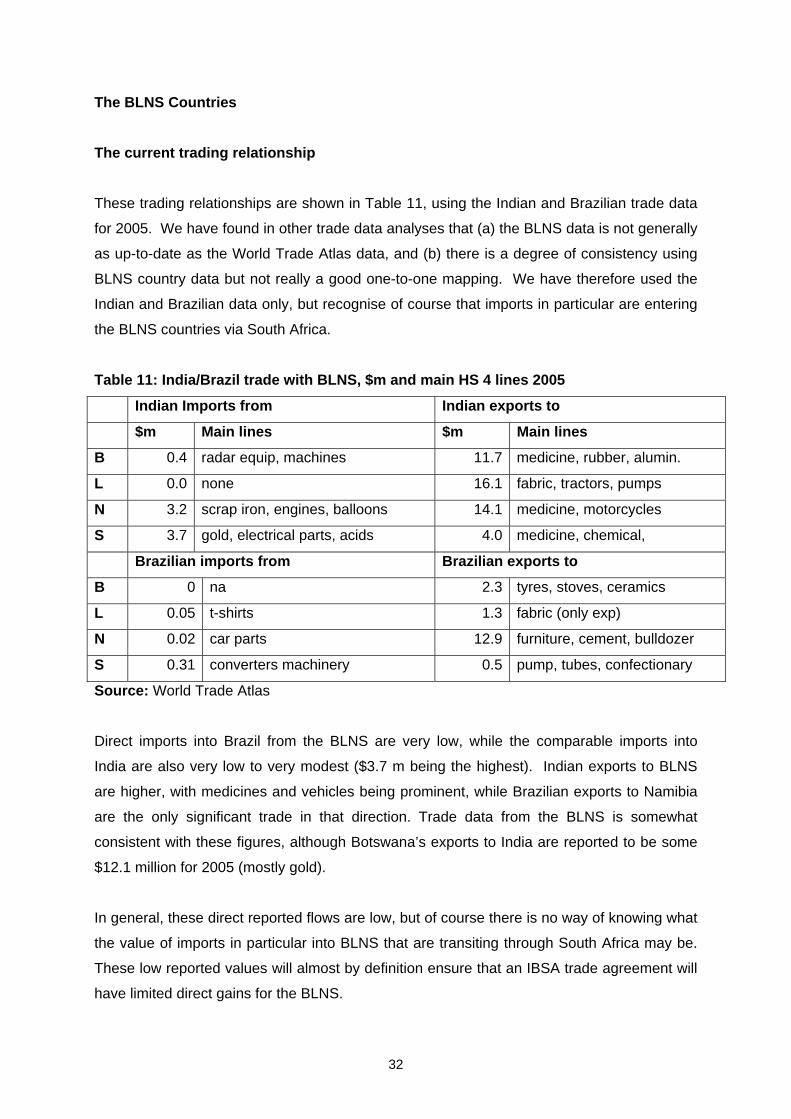
These trading relationships are shown in Table 11, using the Indian and Brazilian trade data

for 2005. We have found in other trade data analyses that (a) the BLNS data is not generally

as up-to-date as the World Trade Atlas data, and (b) there is a degree of consistency using

BLNS country data but not really a good one-to-one mapping. We have therefore used the

Indian and Brazilian data only, but recognise of course that imports in particular are entering

the BLNS countries via South Africa.

Table 11: India/Brazil trade with BLNS, $m and main HS 4 lines 2005

Indian Imports from Indian exports to

$m Main lines $m Main lines

B 0.4 radar equip, machines 11.7 medicine, rubber, alumin.

L 0.0 none 16.1 fabric, tractors, pumps

N 3.2 scrap iron, engines, balloons 14.1 medicine, motorcycles

S 3.7 gold, electrical parts, acids 4.0 medicine, chemical,

Brazilian imports from Brazilian exports to

B 0 na 2.3 tyres, stoves, ceramics

L 0.05 t-shirts 1.3 fabric (only exp)

N 0.02 car parts 12.9 furniture, cement, bulldozer

S 0.31 converters machinery 0.5 pump, tubes, confectionary


Direct imports into Brazil from the BLNS are very low, while the comparable imports into

India are also very low to very modest ($3.7 m being the highest). Indian exports to BLNS

are higher, with medicines and vehicles being prominent, while Brazilian exports to Namibia

are the only significant trade in that direction. Trade data from the BLNS is somewhat

consistent with these figures, although Botswana’s exports to India are reported to be some

$12.1 million for 2005 (mostly gold).

In general, these direct reported flows are low, but of course there is no way of knowing what

the value of imports in particular into BLNS that are transiting through South Africa may be.

These low reported values will almost by definition ensure that an IBSA trade agreement will

have limited direct gains for the BLNS.

33

Section Two: The simulation Introduction Model, database and scenarios

The analysis undertaken in this paper is based upon a variant of the Global Trade Analysis

Project (GTAP)11 model to simulate the impact of possible multilateral market access reforms

resulting from an FTA between the SACU, India and Brazil. The database is the most recent

Version 6 GTAP database with the base year 2001 (Dimaranan et al., 2005), where the 2001

tariff data originated from the Market Access Maps (MacMap) database has been used with

some verification and minor modifications made. The main unskilled labour market closure

of the model has been changed so that the supply of unskilled labor is endogenously

determined by the labor supply elasticity. We believe this is more relevant to a labour-surplus

economy like South Africa’s, although we do sensitivity analysis around this closure to

highlight the policy implications of alternative labor policies.

Like any applied economic model, this model is, of course, based on assumptions, both in

terms of theoretical structure as well as the specific parameters and data used. Regional

production is generated by a constant return to scale technology in a perfectly competitive

environment, and the private demand system is represented by a non-homothetic demand

system (a Constant Difference Elasticity function)12. The foreign trade structure is

characterised by the Armington assumption implying imperfect substitutability between

domestic and foreign goods.

The macroeconomic closure is a neo-classical closure where investments are endogenous

and adjust to accommodate any changes in savings. This approach is adopted at the global

level, and investments are then allocated across regions to equalise the marginal rate of

return in all regions. Although global investments and savings must be equal, this does not

apply at the regional level, where the trade balance is endogenously determined as the

difference between regional savings and regional investments. This is valid as the regional

savings enter the regional utility function. The quantity of endowments (land, skilled labour

and natural resources) in each region is fixed exogenously within the model, although, as

discussed, alternative unskilled labour market assumptions are investigated. The capital 11 See the GTAP website at https://www.gtap.agecon.purdue.edu/ for a full introduction to the model. 12 Hence, the present analysis abstracts from features such as imperfect competition and increasing return to scale, which may, however, be important in certain sectors. We are therefore using what can be thought of as a base GTAP structure.

34

closure adopted in the model is based on the theory where changes in investment levels in

each country/region become on-line instantly, updating the capital stocks endogenously in

the model simulation13. Finally, the numeraire used in the model is a price index of the global

primary factor index.

The global database combines detailed bilateral trade, transport and protection data

characterising economic linkages among regions, together with individual country input-

output data bases which account for intersectoral linkages within regions. The database

contains 96 regions and 57 sectors, and we have aggregated these to 12 regions and 41

sectors in order to keep the model within computational limits and focus on the individual

member countries/regions of the FTA. These 12 regions are (a) the main IBSA parties of

South Africa (ZAF), Botswana (BWA) and Rest of SACU (also called XSC in the model, with

Lesotho, Namibia and Swaziland combined as they are in the GTAP database), India and

Brazil, and (b) another seven country/region grouping of the EU, USA, China, Japan, Nigeria

(NGA), Rest of Africa (RAF) and the Rest of the World (ROW).

The trade data is based upon actual 2001 flows, although tralac has checked and updated

these where practical to 2005 flows. The applied ad valorem equivalents (AVEs) tariff data

found in the standard GTAP version 6 database originate from the Market Access Maps

(MacMap) database, which is compiled from UNCTAD TRAINS data, country notifications to

the WTO, AMAD, and from national customs information (Bouet et al., 2005). The MacMap

database contains bound, MFN and bilateral applied tariff rates (both specific and ad

valorem) at the 6-digit Harmonised Systems (HS6) level. These are than aggregated to

GTAP concordance using trade weights compiled from the COMTRADE database.

Baseline projection 2001 – 2015 A meaningful evaluation of an anticipated policy change can be obtained by comparing the

liberalisation scenario with a non-liberalisation (business as usual) base scenario. This base

must contain projections of the macro-economy and incorporate the effects of important

policy changes other than specific policy changes to be analysed. Our business-as-usual

baseline features a number of important policy initiatives by the EU and others that must be

set in place first. These are (as shown in Box 1):

13 This capital closure adopted in the model is the so called Baldwin closure as documented in GTAP technical paper no. 7.

35

• a stylised implementation of the Agenda 2000 and the Mid-Term Review Reform of the

CAP

• the South Africa EU TDCA agreement

• the abolition of export quotas on textiles and apparel shipped to the EU and the USA

• the accession of China to the WTO

• the final implementation of the UR commitments for developing countries

• the enlargement of the EU with 12 new member countries

• the EBA agreement between LDCs and the EU

• an update of India’s applied MFN rates to the latest year available 2005.14

Box 1. Assumptions shaping the baseline 2001-2015

Projections Shocks to GDP, factor endowments and population

Total factor productivity endogenously determined

Trade Policy changes Implementation of the TDCA agreement between South Africa and the EU

Abolishment of export quotas on textiles and apparel shipped to the EU and the USA

Final implementation of the UR commitments for developing countries

Accession of China to the WTO

Enlargement of the EU customs union and the extension of the EFTA to include the new member

countries

EBA agreement between LDCs and the EU

EU Agenda 2000 and MTR Reform All direct payments deflated by two per cent per year (max budgetary outlays fixed in nominal terms)

Adjusted hectare and livestock premiums (direct payments)

Decoupling of direct payments to a single farm payment

Sugar and milk quotas unchanged

Reductions in intervention prices modelled by reducing export subsidy rates

USA agricultural subsidies Agricultural expenditure fixed in nominal terms at its 2001 level

14 In the process of updating the Indian MFN tariffs it was observed that South Africa exports of coal was classified as import under HS6 code 270112 Bituminous coal in the initial 2001 MacMaps HS6 digit tariff data, while in 2001 to 2005 South Africa was not reporting exports under this code. Therefore the initial MacMaps databases MFN tariff on South African coal exports to India was adjusted to reflect South Africa’s reporting of HS6 digit codes on coal exports.

36

As always, we apply shocks to GDP, population, labour force, and capital to project the world

economy to the baseline year of 2015 – a year when the market access reforms are

assumed to be completed. The projection of the world economy uses the exogenous

assumptions listed in Table 4, and is important in shaping the baseline scenario. The general

sources for these assumptions in Table 12 are given as a footnote to the table, and they

represent the best estimates of the possible future path of these data. The GTAP model

then determines changes in output through both an expansionary and a substitution effect in

each country/region of the model. This expansionary effect represents the effects of growth

in domestic and foreign demand shaped by income and population growth and the assumed

income elasticities, while the substitution effect reflects the changes in competitiveness in

each country/region shaped by changes in relative total factor productivity, cost of production

as well as any policy changes. Thus, the GTAP model uses this set of macroeconomic

projections to generate the ‘best estimate’ of the global production and trade data as it will be

in 2015. Therefore the relative growth rates between each country/region for GDP,

population, labour, capital and total factor productivity play an import role in determining the

relative growth in output of the commodities when projecting the world economy from 2001 to

2015, and we can now take the resulting data set from this baseline simulation as the new

base for our IBSA scenarios. A simulation scenario measures the difference between our

baseline model output at 2015 in the absence of the IBSA against what it would be if IBSA

outcome was introduced with all other factors held constant. Therefore the assumptions

do not really affect the scenario, as the scenario is measured against the baseline that is built

using these assumptions.

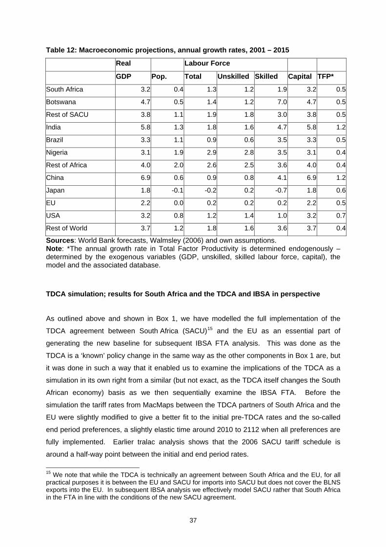
37

Table 12: Macroeconomic projections, annual growth rates, 2001 – 2015

Real Labour Force

GDP Pop. Total Unskilled Skilled Capital TFP*

South Africa 3.2 0.4 1.3 1.2 1.9 3.2 0.5

Botswana 4.7 0.5 1.4 1.2 7.0 4.7 0.5

Rest of SACU 3.8 1.1 1.9 1.8 3.0 3.8 0.5

India 5.8 1.3 1.8 1.6 4.7 5.8 1.2

Brazil 3.3 1.1 0.9 0.6 3.5 3.3 0.5

Nigeria 3.1 1.9 2.9 2.8 3.5 3.1 0.4

Rest of Africa 4.0 2.0 2.6 2.5 3.6 4.0 0.4

China 6.9 0.6 0.9 0.8 4.1 6.9 1.2

Japan 1.8 -0.1 -0.2 0.2 -0.7 1.8 0.6

EU 2.2 0.0 0.2 0.2 0.2 2.2 0.5

USA 3.2 0.8 1.2 1.4 1.0 3.2 0.7

Rest of World 3.7 1.2 1.8 1.6 3.6 3.7 0.4

Sources: World Bank forecasts, Walmsley (2006) and own assumptions. Note: *The annual growth rate in Total Factor Productivity is determined endogenously – determined by the exogenous variables (GDP, unskilled, skilled labour force, capital), the model and the associated database. TDCA simulation; results for South Africa and the TDCA and IBSA in perspective

As outlined above and shown in Box 1, we have modelled the full implementation of the

TDCA agreement between South Africa (SACU)15 and the EU as an essential part of

generating the new baseline for subsequent IBSA FTA analysis. This was done as the

TDCA is a ‘known’ policy change in the same way as the other components in Box 1 are, but

it was done in such a way that it enabled us to examine the implications of the TDCA as a

simulation in its own right from a similar (but not exact, as the TDCA itself changes the South

African economy) basis as we then sequentially examine the IBSA FTA. Before the

simulation the tariff rates from MacMaps between the TDCA partners of South Africa and the

EU were slightly modified to give a better fit to the initial pre-TDCA rates and the so-called

end period preferences, a slightly elastic time around 2010 to 2112 when all preferences are

fully implemented. Earlier tralac analysis shows that the 2006 SACU tariff schedule is

around a half-way point between the initial and end period rates.

15 We note that while the TDCA is technically an agreement between South Africa and the EU, for all practical purposes it is between the EU and SACU for imports into SACU but does not cover the BLNS exports into the EU. In subsequent IBSA analysis we effectively model SACU rather that South Africa in the FTA in line with the conditions of the new SACU agreement.

38

Results from this TDCA simulation suggest that the welfare gains to South Africa are around

$495 million, while those to the EU are a greater $838 million. Botswana gains by some

$41 million, while the rest of SACU loses by around $16 million. Later in the paper we will

present and discuss results from the IBSA simulations, but here we will introduce the fact

that the model is saying that a full and comprehensive IBSA FTA is of greater value (in fact

about double the welfare gains) to South Africa than the partial TDCA. This is mainly

because (a) although South Africa gains comprehensive and almost duty-free access into the

EU for non-agricultural products, in general these manufacturing tariffs are modest, thus the

preferences are not that significant, and (b), more importantly, South Africa gains little

preferences into the highly protected European agricultural market from the TDCA.

Conversely, for IBSA South Africa is deemed to have gained comprehensive access into the

relatively highly protected Indian market in particular, thus gaining a considerable advantage

over global competitors.

Of particular interest from the TDCA simulation is the implications for the motor vehicle

sector in South Africa. Here South African production increases by 4.8 percent from the

base, with exports to the EU increasing by 12 percent in response to close to duty-free

access but imports from the EU increasing by a much smaller three percent as there are

almost no preferences granted from South Africa to Europe. Not surprisingly, there is no

discernable production response in Europe to this increased trade. A more comprehensive

report on the TDCA will be given in subsequent tralac research once the actual 2006 trade

data becomes available, as we wish to apply a comprehensive set of analytical tools to this

FTA rather than just a GTAP simulation. Meanwhile, the TDCA is a known fact as far as

South African trade policy is concerned, so it is important to examine the IBSA from that

starting point (although we note that the TDCA is currently being reviewed and may or may

not subsequently change somewhat, but that is another and unknown factor).

IBSA FTA scenarios

The FTA primary scenario considered in this paper entails the result from the removal of

trade barriers between India, Brazil and the member countries of the SACU as measured in

the year 2015 in a world shaped by the baseline scenario. This implies that all ad valorem

tariffs and ad valorem equivalent of specific tariffs between all participating countries India

Brazil and the SACU (IBSA) are abolished. Differences between the so-called baseline

scenario and this so-called primary scenario are therefore the results of implementation of

the IBSA FTA. Note that we are not modelling reductions in either services or any non-tariff

barriers.

39

In addition, it is always possible to do an almost endless number of ‘what if' scenarios. For

this study we have limited these to two basic assumptions/possible outcomes. One is that

there will be a successful conclusion to the Doha Development Round of the WTO, and we

have modelled this using the G20 proposal for agriculture and the NAMA 11 groups

suggestions to formula our Non-Agricultural Market Access reform. Our assumptions used

are:

• In the agricultural case we use:

• the tiered market access formula suggested by the G20 allowing developed countries

take out two percent of their tariff lines as sensitive products while developing

countries are allowed to exclude three percent of their tariff lines.

• all agricultural export subsidies found in the GTAP are eliminated, while there is no

change to domestic support in our Doha scenario.

• the EU has already implemented its MTR reform of the CAP during the base line

while the assumption is made that the few remaining countries that need to make

adjustments can do so by lowering administered prices used in their Aggregate

Measurement of Support (AMS) calculation notified to the WTO without it having any

effect on domestic product.

• With regard to the NAMA reform we use:

• the simple Swiss formula with coefficients 5 and 20 for respectively developed and

developing countries, including newly acceded members.

• Developing countries and newly acceded countries are allowed to exclude up to 5

percent of their tariff lines if it does not exceed five percent of their value of imports.

• Non bound tariff are bound by adding 20 percentage points (mark up) to the MFN

rate.

• The so-called Paragraph 6 countries and small vulnerable countries are not required

to make any reductions in their applied tariffs but have to bind all their tariffs so that

the simple average of all NAMA tariff lines does not exceed 28.5 and 22 percent

respectively on average.

• Less developed countries are not required to do anything but gain duty-free access

into developed countries markets.

The second assumption is that the IBSA negotiators will fail to negotiate a fully

comprehensive FTA, and we have proxied this possibility by assuming the outcome will be a

40

50 percent cut in bilateral tariff rates (S2 below). In reality, it is more likely that sensitive

sectors for either party will be isolated from any final agreement, but we have opted for this

blanket 50 percent option. To complete the picture we have combined these latter two

scenarios into a combined one of a successful WTO Doha round increasing multilateral

market access and the bilateral IBSA FTA.

Operationally, these are represented as follows:

• Firstly, scenario S1 (the primary scenario) is run to simulate the effects of the

comprehensive FTA in a post UR environment where all other known international

commitments are fully implemented.

• Scenario S2, implements the partial FTA with a 50 percent reduction in applied AVE

tariffs between the IBSA countries

• Then Scenario S3 is run. This is an implementation of a stylised outcome of a possible

DDA round of the WTO using the assumptions outlined above.

• Next Scenario S4 extends S3 by also including the post-Doha FTA between IBSA

countries with a 100 per cent removal of AVE tariffs between the FTA countries.

In order to find the isolated effects of creating the FTA in a post DDA round, scenario S3 is

subtracted from scenario S4, quantifying the effect of the FTA. Therefore the results shown

later for the FTA (in an environment where the DDA has been completed) are technically the

results of scenarios (S4 – S3).

Before we introduce the results of the simulations, we will present Table 13 with the tariffs

faced by South Africa into both India and Brazil and by both India and Brazil into South Africa

to give a perspective of the relative protection levels by GTAP sectors. This information is

reproduced in Annex Tables A1 and A2 along with the changes in trade flows as a result of

IBSA. Note that these tariff rates are as used within the GTAP model, and reflect the

differences in individual products within a particular GTAP sector and are therefore not

directly comparable in the case of imports into South Africa. Note that we have not displayed

the zero tariff levels for paddy rice, cane and beet sugar, and raw milk, as these products are

effectively non-traded. The table highlights that there are several sectors in all countries that

have relatively high initial levels of tariff protection.

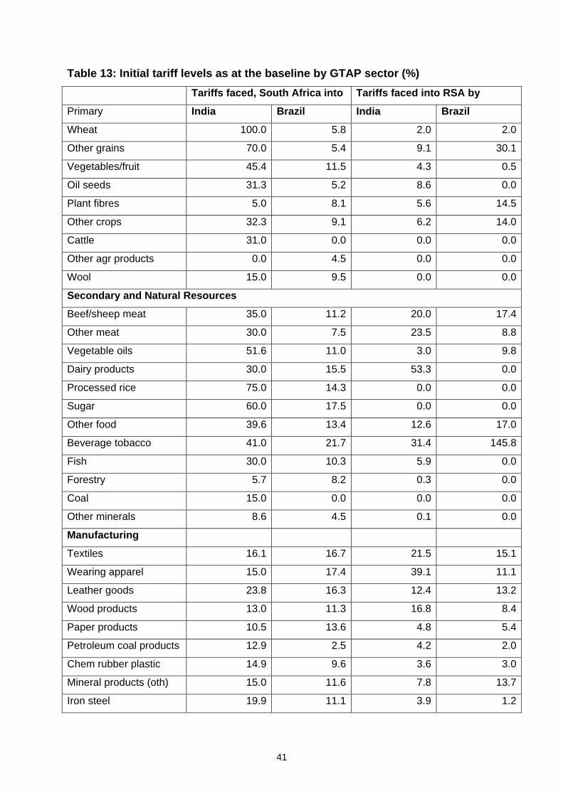
41

Table 13: Initial tariff levels as at the baseline by GTAP sector (%) Tariffs faced, South Africa into Tariffs faced into RSA by

Primary India Brazil India Brazil

Wheat 100.0 5.8 2.0 2.0

Other grains 70.0 5.4 9.1 30.1

Vegetables/fruit 45.4 11.5 4.3 0.5

Oil seeds 31.3 5.2 8.6 0.0

Plant fibres 5.0 8.1 5.6 14.5

Other crops 32.3 9.1 6.2 14.0

Cattle 31.0 0.0 0.0 0.0

Other agr products 0.0 4.5 0.0 0.0

Wool 15.0 9.5 0.0 0.0

Secondary and Natural Resources

Beef/sheep meat 35.0 11.2 20.0 17.4

Other meat 30.0 7.5 23.5 8.8

Vegetable oils 51.6 11.0 3.0 9.8

Dairy products 30.0 15.5 53.3 0.0

Processed rice 75.0 14.3 0.0 0.0

Sugar 60.0 17.5 0.0 0.0

Other food 39.6 13.4 12.6 17.0

Beverage tobacco 41.0 21.7 31.4 145.8

Fish 30.0 10.3 5.9 0.0

Forestry 5.7 8.2 0.3 0.0

Coal 15.0 0.0 0.0 0.0

Other minerals 8.6 4.5 0.1 0.0

Manufacturing

Textiles 16.1 16.7 21.5 15.1

Wearing apparel 15.0 17.4 39.1 11.1

Leather goods 23.8 16.3 12.4 13.2

Wood products 13.0 11.3 16.8 8.4

Paper products 10.5 13.6 4.8 5.4

Petroleum coal products 12.9 2.5 4.2 2.0

Chem rubber plastic 14.9 9.6 3.6 3.0

Mineral products (oth) 15.0 11.6 7.8 13.7

Iron steel 19.9 11.1 3.9 1.2

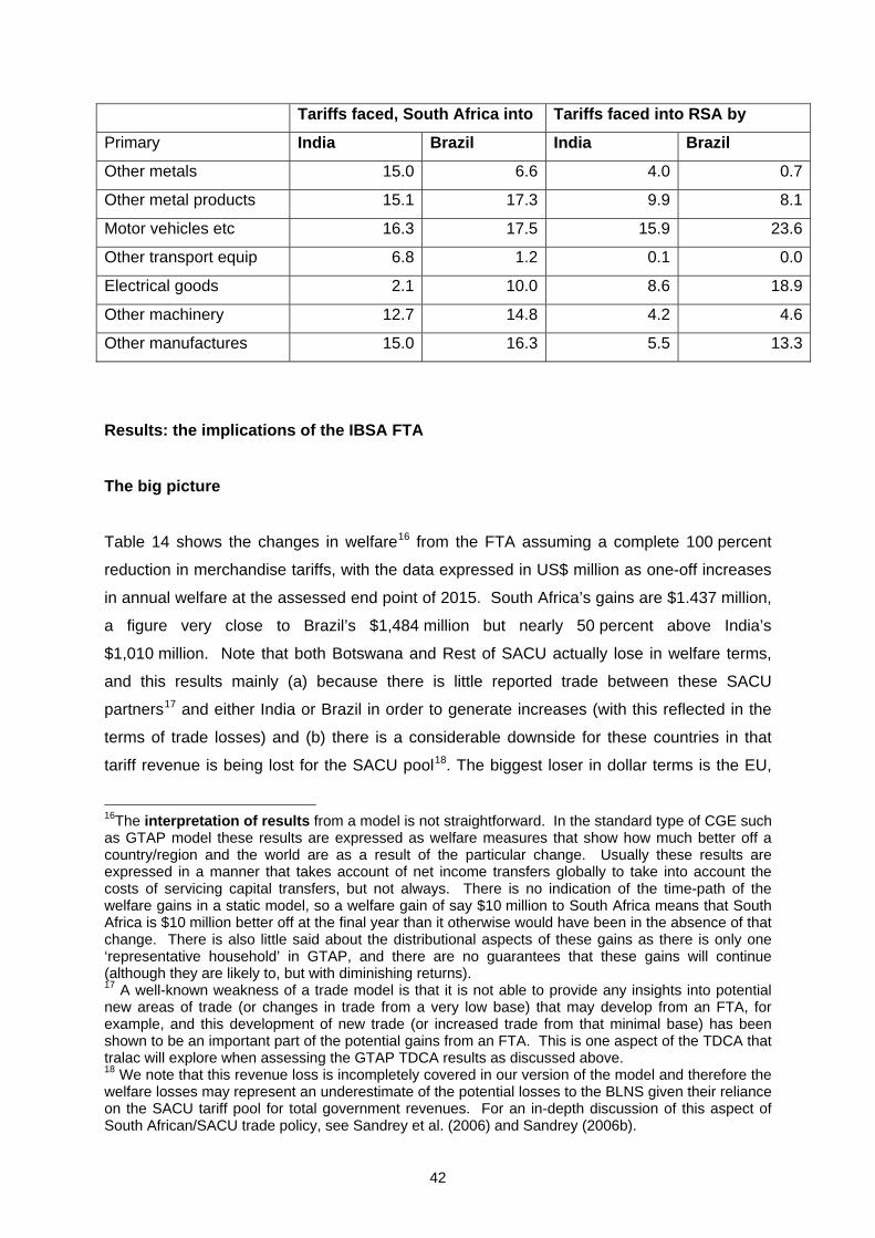
42

Tariffs faced, South Africa into Tariffs faced into RSA by

Primary India Brazil India Brazil

Other metals 15.0 6.6 4.0 0.7

Other metal products 15.1 17.3 9.9 8.1

Motor vehicles etc 16.3 17.5 15.9 23.6

Other transport equip 6.8 1.2 0.1 0.0

Electrical goods 2.1 10.0 8.6 18.9

Other machinery 12.7 14.8 4.2 4.6

Other manufactures 15.0 16.3 5.5 13.3

Results: the implications of the IBSA FTA The big picture

Table 14 shows the changes in welfare16 from the FTA assuming a complete 100 percent

reduction in merchandise tariffs, with the data expressed in US$ million as one-off increases

in annual welfare at the assessed end point of 2015. South Africa’s gains are $1.437 million,

a figure very close to Brazil’s $1,484 million but nearly 50 percent above India’s

$1,010 million. Note that both Botswana and Rest of SACU actually lose in welfare terms,

and this results mainly (a) because there is little reported trade between these SACU

partners17 and either India or Brazil in order to generate increases (with this reflected in the

terms of trade losses) and (b) there is a considerable downside for these countries in that

tariff revenue is being lost for the SACU pool18. The biggest loser in dollar terms is the EU,

16The interpretation of results from a model is not straightforward. In the standard type of CGE such as GTAP model these results are expressed as welfare measures that show how much better off a country/region and the world are as a result of the particular change. Usually these results are expressed in a manner that takes account of net income transfers globally to take into account the costs of servicing capital transfers, but not always. There is no indication of the time-path of the welfare gains in a static model, so a welfare gain of say $10 million to South Africa means that South Africa is $10 million better off at the final year than it otherwise would have been in the absence of that change. There is also little said about the distributional aspects of these gains as there is only one ‘representative household’ in GTAP, and there are no guarantees that these gains will continue (although they are likely to, but with diminishing returns). 17 A well-known weakness of a trade model is that it is not able to provide any insights into potential new areas of trade (or changes in trade from a very low base) that may develop from an FTA, for example, and this development of new trade (or increased trade from that minimal base) has been shown to be an important part of the potential gains from an FTA. This is one aspect of the TDCA that tralac will explore when assessing the GTAP TDCA results as discussed above. 18 We note that this revenue loss is incompletely covered in our version of the model and therefore the welfare losses may represent an underestimate of the potential losses to the BLNS given their reliance on the SACU tariff pool for total government revenues. For an in-depth discussion of this aspect of South African/SACU trade policy, see Sandrey et al. (2006) and Sandrey (2006b).

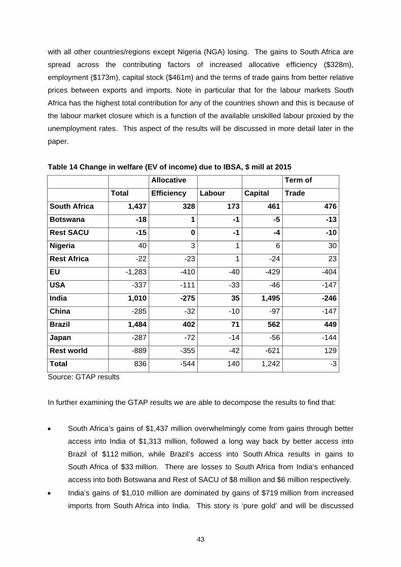
43

with all other countries/regions except Nigeria (NGA) losing. The gains to South Africa are

spread across the contributing factors of increased allocative efficiency ($328m),

employment ($173m), capital stock ($461m) and the terms of trade gains from better relative

prices between exports and imports. Note in particular that for the labour markets South

Africa has the highest total contribution for any of the countries shown and this is because of

the labour market closure which is a function of the available unskilled labour proxied by the

unemployment rates. This aspect of the results will be discussed in more detail later in the

paper.

Table 14 Change in welfare (EV of income) due to IBSA, $ mill at 2015

Allocative Term of

Total Efficiency Labour Capital Trade

South Africa 1,437 328 173 461 476

Botswana -18 1 -1 -5 -13

Rest SACU -15 0 -1 -4 -10

Nigeria 40 3 1 6 30

Rest Africa -22 -23 1 -24 23

EU -1,283 -410 -40 -429 -404

USA -337 -111 -33 -46 -147

India 1,010 -275 35 1,495 -246

China -285 -32 -10 -97 -147

Brazil 1,484 402 71 562 449

Japan -287 -72 -14 -56 -144

Rest world -889 -355 -42 -621 129

Total 836 -544 140 1,242 -3

Source: GTAP results

In further examining the GTAP results we are able to decompose the results to find that:

• South Africa’s gains of $1,437 million overwhelmingly come from gains through better

access into India of $1,313 million, followed a long way back by better access into

Brazil of $112 million, while Brazil’s access into South Africa results in gains to

South Africa of $33 million. There are losses to South Africa from India’s enhanced

access into both Botswana and Rest of SACU of $8 million and $6 million respectively.

• India’s gains of $1,010 million are dominated by gains of $719 million from increased

imports from South Africa into India. This story is ‘pure gold’ and will be discussed

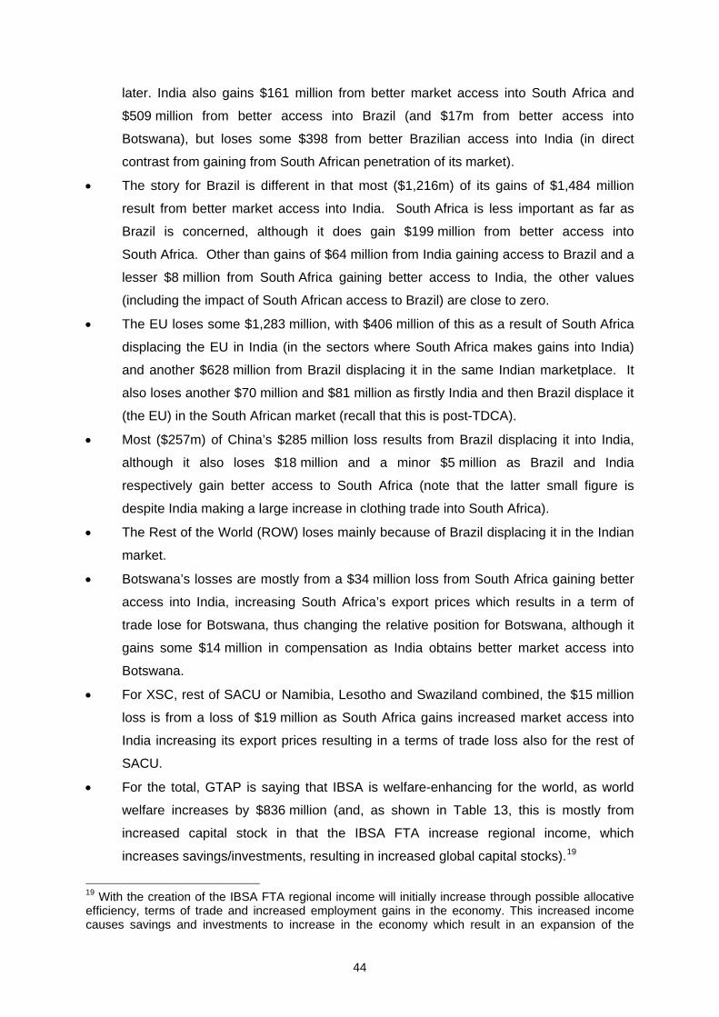
44

later. India also gains $161 million from better market access into South Africa and

$509 million from better access into Brazil (and $17m from better access into

Botswana), but loses some $398 from better Brazilian access into India (in direct

contrast from gaining from South African penetration of its market).

• The story for Brazil is different in that most ($1,216m) of its gains of $1,484 million

result from better market access into India. South Africa is less important as far as

Brazil is concerned, although it does gain $199 million from better access into

South Africa. Other than gains of $64 million from India gaining access to Brazil and a

lesser $8 million from South Africa gaining better access to India, the other values

(including the impact of South African access to Brazil) are close to zero.

• The EU loses some $1,283 million, with $406 million of this as a result of South Africa

displacing the EU in India (in the sectors where South Africa makes gains into India)

and another $628 million from Brazil displacing it in the same Indian marketplace. It

also loses another $70 million and $81 million as firstly India and then Brazil displace it

(the EU) in the South African market (recall that this is post-TDCA).

• Most ($257m) of China’s $285 million loss results from Brazil displacing it into India,

although it also loses $18 million and a minor $5 million as Brazil and India

respectively gain better access to South Africa (note that the latter small figure is

despite India making a large increase in clothing trade into South Africa).

• The Rest of the World (ROW) loses mainly because of Brazil displacing it in the Indian

market.

• Botswana’s losses are mostly from a $34 million loss from South Africa gaining better

access into India, increasing South Africa’s export prices which results in a term of

trade lose for Botswana, thus changing the relative position for Botswana, although it

gains some $14 million in compensation as India obtains better market access into

Botswana.

• For XSC, rest of SACU or Namibia, Lesotho and Swaziland combined, the $15 million

loss is from a loss of $19 million as South Africa gains increased market access into

India increasing its export prices resulting in a terms of trade loss also for the rest of

SACU.

• For the total, GTAP is saying that IBSA is welfare-enhancing for the world, as world

welfare increases by $836 million (and, as shown in Table 13, this is mostly from

increased capital stock in that the IBSA FTA increase regional income, which

increases savings/investments, resulting in increased global capital stocks).19

19 With the creation of the IBSA FTA regional income will initially increase through possible allocative efficiency, terms of trade and increased employment gains in the economy. This increased income causes savings and investments to increase in the economy which result in an expansion of the

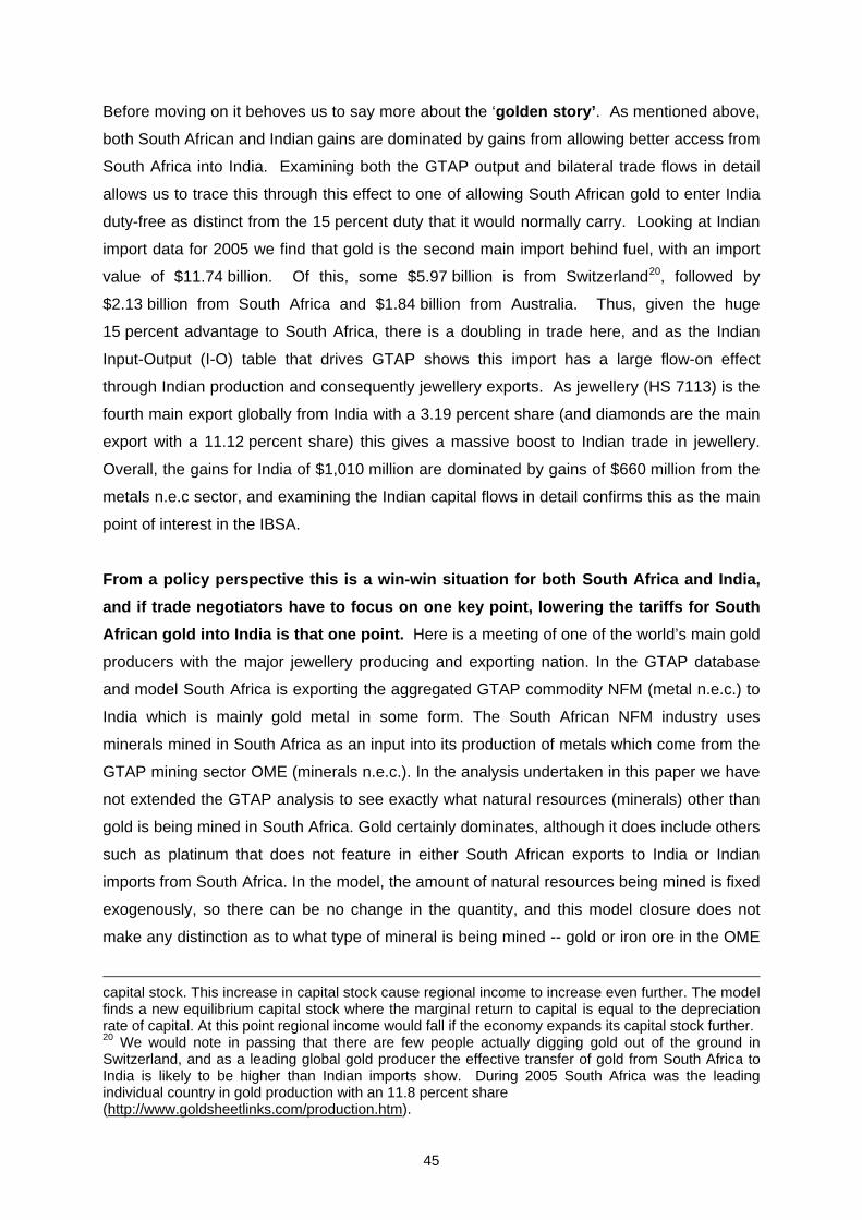
45

Before moving on it behoves us to say more about the ‘golden story’. As mentioned above,

both South African and Indian gains are dominated by gains from allowing better access from

South Africa into India. Examining both the GTAP output and bilateral trade flows in detail

allows us to trace this through this effect to one of allowing South African gold to enter India

duty-free as distinct from the 15 percent duty that it would normally carry. Looking at Indian

import data for 2005 we find that gold is the second main import behind fuel, with an import

value of $11.74 billion. Of this, some $5.97 billion is from Switzerland20, followed by

$2.13 billion from South Africa and $1.84 billion from Australia. Thus, given the huge

15 percent advantage to South Africa, there is a doubling in trade here, and as the Indian

Input-Output (I-O) table that drives GTAP shows this import has a large flow-on effect

through Indian production and consequently jewellery exports. As jewellery (HS 7113) is the

fourth main export globally from India with a 3.19 percent share (and diamonds are the main

export with a 11.12 percent share) this gives a massive boost to Indian trade in jewellery.

Overall, the gains for India of $1,010 million are dominated by gains of $660 million from the

metals n.e.c sector, and examining the Indian capital flows in detail confirms this as the main

point of interest in the IBSA.

From a policy perspective this is a win-win situation for both South Africa and India, and if trade negotiators have to focus on one key point, lowering the tariffs for South African gold into India is that one point. Here is a meeting of one of the world’s main gold

producers with the major jewellery producing and exporting nation. In the GTAP database

and model South Africa is exporting the aggregated GTAP commodity NFM (metal n.e.c.) to

India which is mainly gold metal in some form. The South African NFM industry uses

minerals mined in South Africa as an input into its production of metals which come from the

GTAP mining sector OME (minerals n.e.c.). In the analysis undertaken in this paper we have

not extended the GTAP analysis to see exactly what natural resources (minerals) other than

gold is being mined in South Africa. Gold certainly dominates, although it does include others

such as platinum that does not feature in either South African exports to India or Indian

imports from South Africa. In the model, the amount of natural resources being mined is fixed

exogenously, so there can be no change in the quantity, and this model closure does not

make any distinction as to what type of mineral is being mined -- gold or iron ore in the OME

capital stock. This increase in capital stock cause regional income to increase even further. The model finds a new equilibrium capital stock where the marginal return to capital is equal to the depreciation rate of capital. At this point regional income would fall if the economy expands its capital stock further. 20 We would note in passing that there are few people actually digging gold out of the ground in Switzerland, and as a leading global gold producer the effective transfer of gold from South Africa to India is likely to be higher than Indian imports show. During 2005 South Africa was the leading individual country in gold production with an 11.8 percent share (http://www.goldsheetlinks.com/production.htm).

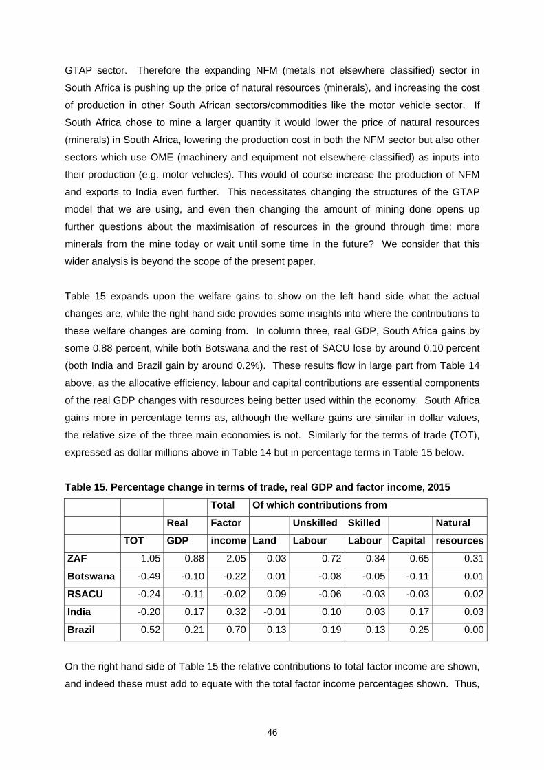
46

GTAP sector. Therefore the expanding NFM (metals not elsewhere classified) sector in

South Africa is pushing up the price of natural resources (minerals), and increasing the cost

of production in other South African sectors/commodities like the motor vehicle sector. If

South Africa chose to mine a larger quantity it would lower the price of natural resources

(minerals) in South Africa, lowering the production cost in both the NFM sector but also other

sectors which use OME (machinery and equipment not elsewhere classified) as inputs into

their production (e.g. motor vehicles). This would of course increase the production of NFM

and exports to India even further. This necessitates changing the structures of the GTAP

model that we are using, and even then changing the amount of mining done opens up

further questions about the maximisation of resources in the ground through time: more

minerals from the mine today or wait until some time in the future? We consider that this

wider analysis is beyond the scope of the present paper.

Table 15 expands upon the welfare gains to show on the left hand side what the actual

changes are, while the right hand side provides some insights into where the contributions to

these welfare changes are coming from. In column three, real GDP, South Africa gains by

some 0.88 percent, while both Botswana and the rest of SACU lose by around 0.10 percent

(both India and Brazil gain by around 0.2%). These results flow in large part from Table 14

above, as the allocative efficiency, labour and capital contributions are essential components

of the real GDP changes with resources being better used within the economy. South Africa

gains more in percentage terms as, although the welfare gains are similar in dollar values,

the relative size of the three main economies is not. Similarly for the terms of trade (TOT),

expressed as dollar millions above in Table 14 but in percentage terms in Table 15 below.

Table 15. Percentage change in terms of trade, real GDP and factor income, 2015

Total Of which contributions from

Real Factor Unskilled Skilled Natural

TOT GDP income Land Labour Labour Capital resources

ZAF 1.05 0.88 2.05 0.03 0.72 0.34 0.65 0.31

Botswana -0.49 -0.10 -0.22 0.01 -0.08 -0.05 -0.11 0.01

RSACU -0.24 -0.11 -0.02 0.09 -0.06 -0.03 -0.03 0.02

India -0.20 0.17 0.32 -0.01 0.10 0.03 0.17 0.03

Brazil 0.52 0.21 0.70 0.13 0.19 0.13 0.25 0.00

On the right hand side of Table 15 the relative contributions to total factor income are shown,

and indeed these must add to equate with the total factor income percentages shown. Thus,

47

for South Africa’s 2.05 percentage increases in total factor income, 0.03 percent is coming

from better land use, 0.72 percent from enhanced unskilled labour, 0.34 percent from skilled

labour, 0.65 percent from capital and the final 0.31 percent from the natural resource base.

Note that for land, skilled labour and natural resources, the quantities are fixed in the GTAP

model, so the increases are coming from price increases as their values are bidded up, while

for both unskilled labour and capital where the quantities are not fixed there is both a price

and a quantity effect. The unskilled labour story will be examined in more detail later under

alternative model closures, as these policy options for (a) holding unskilled labour fixed and

raising the wage rate, (b) holding the wage rate fixed and increasing the people in

employment and (c) some intermediate position are crucial policy questions for South Africa.

Currently we are using a closure of (c) as discussed earlier.

Changes in trade flows

The details of changes to South Africa’s trading patterns are shown in Annex A, with exports

in Annex Table A1 and imports in Annex Table A2 respectively. These tables split the GTAP

sectors into primary and secondary agriculture, natural resource and manufacturing before

displaying (a) the AVE or the initial pre-FTA average ad valorem tariff facing either South

African exports in the partner market for exports or partner tariffs into South Africa for

imports, and (b) the change in either South African exports or imports into or from the

respective country/regions in response to reducing these border tariffs to zero. These trade

flow changes are given in both US dollar values and percentage changes from the base to

put them in perspective. The markets for exports from and sources of imports into South

Africa are provided as India, Brazil, the rest of SACU (with Botswana and XSA combined)

and the rest of the world with all others combined rather than the ROW used in the model.

There are also two columns on the right hand side showing the total overall changes by

value and percentage change.

Table 16 shows the aggregate overall changes to trade flows for the partner countries in

2015, expressed as percentage changes for both exports and imports and then in US$

million for the trade balance. The clear gainer is South Africa, with increased exports

globally, once all markets are accounted for of $251 million, while India and Brazil faces

losses of some $392 million and $54 million respectively as increased exports are less than

the import changes. Botswana has a deteriorating trade balance of $4 million21, while the

21 Note that Table 14 refers to a deteriorating terms of trade (TOT) for Botswana, while Table 16 shows the actual trade flows. They are different concepts, as TOT is the relative indicator price of exports and imports.

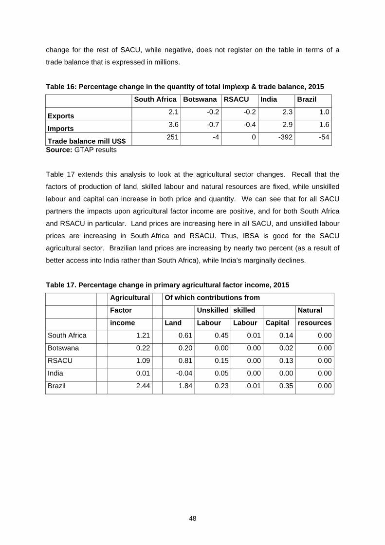
48

change for the rest of SACU, while negative, does not register on the table in terms of a

trade balance that is expressed in millions.

Table 16: Percentage change in the quantity of total imp\exp & trade balance, 2015

South Africa Botswana RSACU India Brazil

Exports 2.1 -0.2 -0.2 2.3 1.0

Imports 3.6 -0.7 -0.4 2.9 1.6

Trade balance mill US$ 251 -4 0 -392 -54


Table 17 extends this analysis to look at the agricultural sector changes. Recall that the

factors of production of land, skilled labour and natural resources are fixed, while unskilled

labour and capital can increase in both price and quantity. We can see that for all SACU

partners the impacts upon agricultural factor income are positive, and for both South Africa

and RSACU in particular. Land prices are increasing here in all SACU, and unskilled labour

prices are increasing in South Africa and RSACU. Thus, IBSA is good for the SACU

agricultural sector. Brazilian land prices are increasing by nearly two percent (as a result of

better access into India rather than South Africa), while India’s marginally declines.

Table 17. Percentage change in primary agricultural factor income, 2015

Agricultural Of which contributions from

Factor Unskilled skilled Natural

income Land Labour Labour Capital resources

South Africa 1.21 0.61 0.45 0.01 0.14 0.00

Botswana 0.22 0.20 0.00 0.00 0.02 0.00

RSACU 1.09 0.81 0.15 0.00 0.13 0.00

India 0.01 -0.04 0.05 0.00 0.00 0.00

Brazil 2.44 1.84 0.23 0.01 0.35 0.00

49

The specific sector results

This section will discuss the production, trade and relative prices changes in the GTAP

sectors. The following series of tables examining the changes to South African trade

flows is largely drawn from the Annex A tables. We will start with the agricultural and natural resource sectors to keep the analysis

manageable, and these are shown in Table 18. Keep in mind that these are percentage

changes, and some of these may be off low bases. Further analysis of the results (see

Annex Table A1) shows that in the agricultural sector South Africa increases exports to

India by $184 million and Brazil by a much lesser $7 million, but overall some $144 million of

this is at the expense of exports to other SACU ($4 million less) and the rest of the world.

Thus, the total increase is only $46 million. Of the total increase, most is in vegetable oils

and fats ($69m) and wool (29m) where big increases to India take place, while there are

global reductions of $18 million each in exports of (a) vegetables, fruit and nuts and (b) other

food products. For imports, there is a similar but slightly larger overall increase of

$93 million, driven mostly by increased imports from Brazil of $75 million (other crops, other

meats and vegetable oils and fats). In the natural resources sector, there is an increase of

$190 million globally, dominated by coal products of $179 million as the percentage changes

shown in coal are off large bases. Exports of coal to India increase by some $824 million

(over 500%) as the duty rates of 15 percent are slashed, and this necessitates imports into

South Africa from the rest of the world as South Africa’s relative price increases

domestically22. In summary, there is little action in either exports or imports in the agricultural sectors, and therefore limited production changes, while only coal products show increased trade in the natural resources sectors.

The interpretation of Table 18 is as follows, using wheat as an example. The table shows

that real wheat prices actually increase by 0.8 percent (right hand column). This however

does not seem to be enough to attract resources into wheat production as other sectors (in

both agriculture and NAMA) become relatively more profitable. Consequently, imports of

wheat rise by 2.3 percent and exports decline by 2.0 percent. This leads to a final decline of

0.8 percent in South African wheat production as a result of IBSA.

22 Once again the quantity of coal being extracted from the mines in South Africa is fixed exogenously in the model, therefore the increased demand of coal by India increases the South African coal price but with no change in the quantity mined.

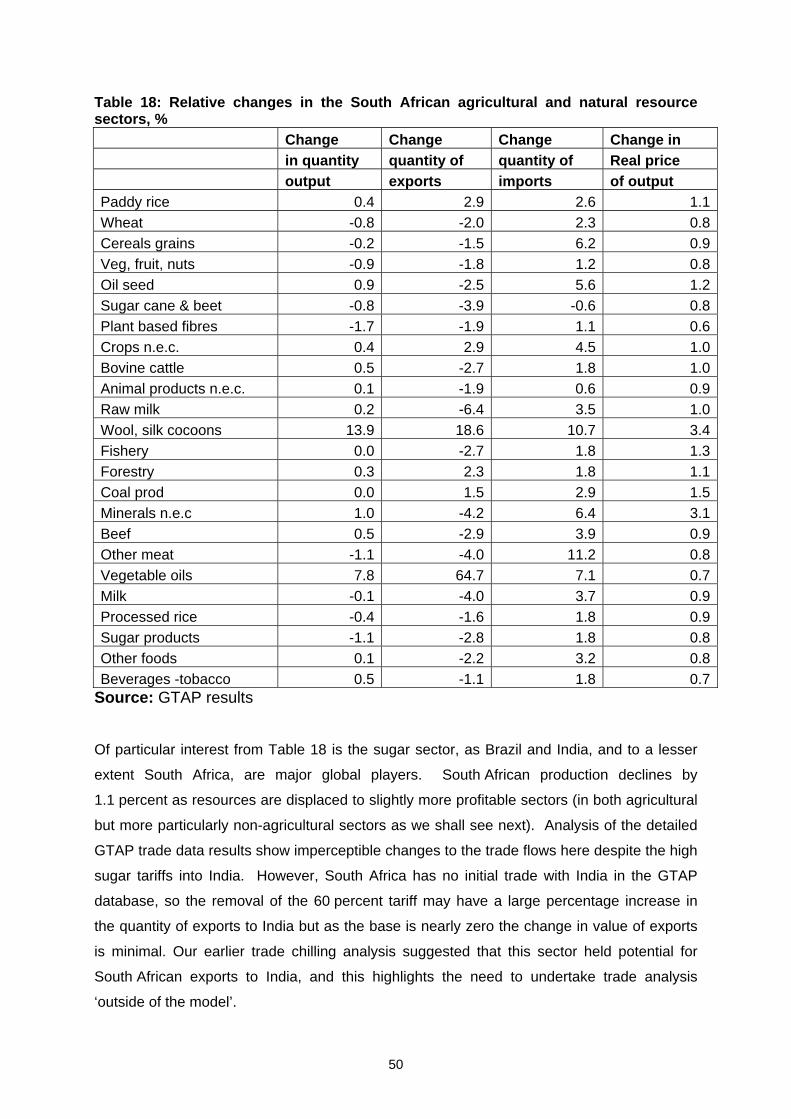
50

Table 18: Relative changes in the South African agricultural and natural resource sectors, % Change Change Change Change in in quantity quantity of quantity of Real price output exports imports of output Paddy rice 0.4 2.9 2.6 1.1Wheat -0.8 -2.0 2.3 0.8Cereals grains -0.2 -1.5 6.2 0.9Veg, fruit, nuts -0.9 -1.8 1.2 0.8Oil seed 0.9 -2.5 5.6 1.2Sugar cane & beet -0.8 -3.9 -0.6 0.8Plant based fibres -1.7 -1.9 1.1 0.6Crops n.e.c. 0.4 2.9 4.5 1.0Bovine cattle 0.5 -2.7 1.8 1.0Animal products n.e.c. 0.1 -1.9 0.6 0.9Raw milk 0.2 -6.4 3.5 1.0Wool, silk cocoons 13.9 18.6 10.7 3.4Fishery 0.0 -2.7 1.8 1.3Forestry 0.3 2.3 1.8 1.1Coal prod 0.0 1.5 2.9 1.5Minerals n.e.c 1.0 -4.2 6.4 3.1Beef 0.5 -2.9 3.9 0.9Other meat -1.1 -4.0 11.2 0.8Vegetable oils 7.8 64.7 7.1 0.7Milk -0.1 -4.0 3.7 0.9Processed rice -0.4 -1.6 1.8 0.9Sugar products -1.1 -2.8 1.8 0.8Other foods 0.1 -2.2 3.2 0.8Beverages -tobacco 0.5 -1.1 1.8 0.7


Of particular interest from Table 18 is the sugar sector, as Brazil and India, and to a lesser

extent South Africa, are major global players. South African production declines by

1.1 percent as resources are displaced to slightly more profitable sectors (in both agricultural

but more particularly non-agricultural sectors as we shall see next). Analysis of the detailed

GTAP trade data results show imperceptible changes to the trade flows here despite the high

sugar tariffs into India. However, South Africa has no initial trade with India in the GTAP

database, so the removal of the 60 percent tariff may have a large percentage increase in

the quantity of exports to India but as the base is nearly zero the change in value of exports

is minimal. Our earlier trade chilling analysis suggested that this sector held potential for

South African exports to India, and this highlights the need to undertake trade analysis

‘outside of the model’.

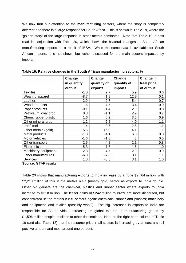
51

We now turn our attention to the manufacturing sectors, where the story is completely

different and there is a large response for South Africa. This is shown in Table 19, where the

‘golden story’ of the large response in other metals dominates. Note that Table 19 is best

read in conjunction with Table 20, which shows the bilateral changes to South African

manufacturing exports as a result of IBSA. While the same data is available for South

African imports, it is not shown but rather discussed for the main sectors impacted by

imports.

Table 19: Relative changes in the South African manufacturing sectors, %

Change Change Change Change in in quantity quantity of quantity of Real price output exports imports of output Textiles -1.0 2.7 5.9 0.6Wearing apparel -8.7 -1.9 12.9 0.1Leather -2.9 -2.7 5.4 0.7Wood products -1.6 -4.5 3.4 0.9Paper products -0.1 -1.4 2.9 0.8Petroleum, coal prod 0.3 -1.1 2.9 0.7Chem, rubber plastic 1.6 6.2 3.5 0.9Other mineral prod -1.2 -2.5 4.0 1.1Iron/steel -1.4 -0.5 2.5 1.1Other metals (gold) 15.5 16.9 14.1 1.1Metal products -1.8 -4.1 6.8 0.8Motor vehicles -1.6 -1.8 4.3 0.5Other transport -2.5 -4.2 2.1 0.8Electronics -5.3 -7.6 1.5 1.0Machinery equipment -2.8 -4.7 2.9 0.9Other manufactures -6.8 -7.8 3.1 1.1Services 1.0 -3.5 3.1 1.0


Table 20 shows that manufacturing exports to India increase by a huge $2,764 million, with

$2,213 million of this in the metals n.e.c (mostly gold) sector as exports to India double.

Other big gainers are the chemical, plastics and rubber sector where exports to India

increase by $318 million. The lesser gains of $242 million to Brazil are more dispersed, but

concentrated in the metals n.e.c. sectors again: chemicals, rubber and plastics; machinery

and equipment; and textiles (possibly wool?). The big increases in exports to India are

responsible for South Africa increasing its global exports of manufacturing goods by

$1,596 million despite declines to other destinations. Note on the right hand column of Table

19 (and also Table 18) that the resource price in all sectors is increasing by at least a small

positive amount and most around one percent.

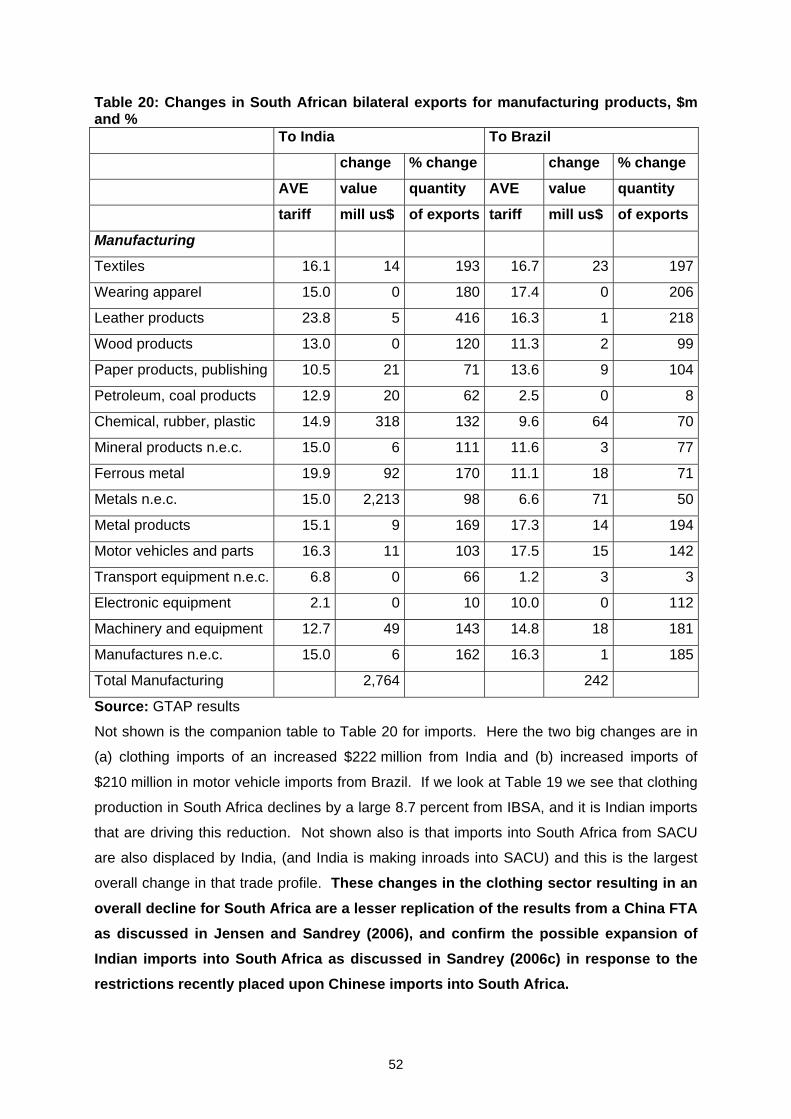
52

Table 20: Changes in South African bilateral exports for manufacturing products, $m and % To India To Brazil

change % change change % change

AVE value quantity AVE value quantity

tariff mill us$ of exports tariff mill us$ of exports

Manufacturing

Textiles 16.1 14 193 16.7 23 197

Wearing apparel 15.0 0 180 17.4 0 206

Leather products 23.8 5 416 16.3 1 218

Wood products 13.0 0 120 11.3 2 99

Paper products, publishing 10.5 21 71 13.6 9 104

Petroleum, coal products 12.9 20 62 2.5 0 8

Chemical, rubber, plastic 14.9 318 132 9.6 64 70

Mineral products n.e.c. 15.0 6 111 11.6 3 77

Ferrous metal 19.9 92 170 11.1 18 71

Metals n.e.c. 15.0 2,213 98 6.6 71 50

Metal products 15.1 9 169 17.3 14 194

Motor vehicles and parts 16.3 11 103 17.5 15 142

Transport equipment n.e.c. 6.8 0 66 1.2 3 3

Electronic equipment 2.1 0 10 10.0 0 112

Machinery and equipment 12.7 49 143 14.8 18 181

Manufactures n.e.c. 15.0 6 162 16.3 1 185

Total Manufacturing 2,764 242


Not shown is the companion table to Table 20 for imports. Here the two big changes are in

(a) clothing imports of an increased $222 million from India and (b) increased imports of

$210 million in motor vehicle imports from Brazil. If we look at Table 19 we see that clothing

production in South Africa declines by a large 8.7 percent from IBSA, and it is Indian imports

that are driving this reduction. Not shown also is that imports into South Africa from SACU

are also displaced by India, (and India is making inroads into SACU) and this is the largest

overall change in that trade profile. These changes in the clothing sector resulting in an

overall decline for South Africa are a lesser replication of the results from a China FTA as discussed in Jensen and Sandrey (2006), and confirm the possible expansion of Indian imports into South Africa as discussed in Sandrey (2006c) in response to the restrictions recently placed upon Chinese imports into South Africa.

53

There are several factors in play with respect to the South African motor vehicle (MHV)

sector. Global imports increase by $145 million, mostly through increases from Brazil

($210m) and India ($41m) in response to South African tariffs on current trade of 33.6 and

15.9 percent for Brazil and India respectively going to zero. This new IBSA trade displaces

some $103 million in imports from the rest of the world. Conversely, since the initial export values to India and Brazil were low, there are limited compensating exports to India of

$11 million and Brazil $15 million that do not match the declines to the rest of the world of

$65 million. Overall production in the motor vehicle sector declines by 1.6 percent, as

shown in Table 18. Importantly, the main cause of this 1.6 percent decline is the increased

export (production) of NFM to India pushing up the price of the intermediate inputs

(especially OME) and endowments (labour capital) into the MHV sector which then reduces

MVH production by 1.3 percent. This leaves a reduction of a lesser 0.3 percent by other

effects. This increased price of the intermediate inputs and endowments in the MVH sector

increasing production prices in South Africa also explains the reduction in exports to the Rest

of the World due to increase production costs. This does not necessarily mean that the

South African MVH industry is less efficient than India’s or Brazil’s, but rather that the

industry now has to pay a higher price domestically for inputs.

The labour market closure and alternative scenarios

We believe that this particular section of the GTAP analysis of IBSA potentially makes an

important contribution to the nexus between trade policy and welfare redistribution in

South Africa. The results in this paper are driven from the labour market assumption as

displayed in rows (B) in Table 21 below, with the mathematical derivation of the equation

shown in Annex B to ensure readers that it is both mathematically correct and economically

sensible.

The simulation results as presented above are those given in section (B) of Table 21, where

the welfare gains for South Africa are some $1,437 million and the increased real GDP is

0.88 percent. Not shown earlier is that IBSA, all other things held constant, will contribute a

further 0.69 percent to South Africa’s CPI or inflation rate. This is of course having an impact

upon the whole economy and results in South Africa losing some competitive advantage

globally. The key employment story is that shown in the centre of the table under ZAF,

where the South African story on unskilled labour is told (recall that the supply of skilled

labour is held fixed). Under this closure whereby the unskilled labour supply is a function of

the unemployment rate the employment of unskilled labour increases by 0.46 percent and

the real wage rate by 1.28 percent. To the right of this we see that both employment and the

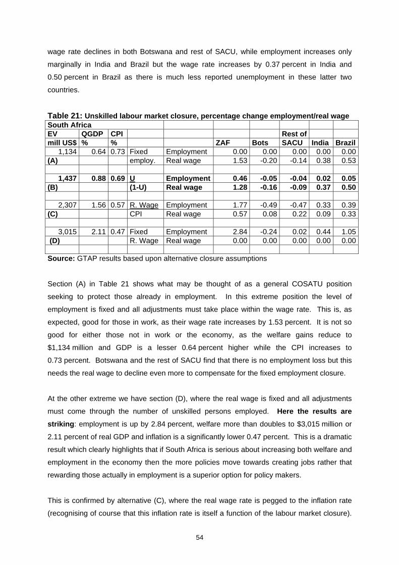
54

wage rate declines in both Botswana and rest of SACU, while employment increases only

marginally in India and Brazil but the wage rate increases by 0.37 percent in India and

0.50 percent in Brazil as there is much less reported unemployment in these latter two

countries.

Table 21: Unskilled labour market closure, percentage change employment/real wage South Africa EV QGDP CPI Rest of mill US$ % % ZAF Bots SACU India Brazil

1,134 0.64 0.73 Fixed Employment 0.00 0.00 0.00 0.00 0.00(A) employ. Real wage 1.53 -0.20 -0.14 0.38 0.53

1,437 0.88 0.69 U Employment 0.46 -0.05 -0.04 0.02 0.05(B) (1-U) Real wage 1.28 -0.16 -0.09 0.37 0.50

2,307 1.56 0.57 R. Wage Employment 1.77 -0.49 -0.47 0.33 0.39(C) CPI Real wage 0.57 0.08 0.22 0.09 0.33

3,015 2.11 0.47 Fixed Employment 2.84 -0.24 0.02 0.44 1.05 (D) R. Wage Real wage 0.00 0.00 0.00 0.00 0.00 Source: GTAP results based upon alternative closure assumptions

Section (A) in Table 21 shows what may be thought of as a general COSATU position

seeking to protect those already in employment. In this extreme position the level of

employment is fixed and all adjustments must take place within the wage rate. This is, as

expected, good for those in work, as their wage rate increases by 1.53 percent. It is not so

good for either those not in work or the economy, as the welfare gains reduce to

$1,134 million and GDP is a lesser 0.64 percent higher while the CPI increases to

0.73 percent. Botswana and the rest of SACU find that there is no employment loss but this

needs the real wage to decline even more to compensate for the fixed employment closure.

At the other extreme we have section (D), where the real wage is fixed and all adjustments

must come through the number of unskilled persons employed. Here the results are striking: employment is up by 2.84 percent, welfare more than doubles to $3,015 million or

2.11 percent of real GDP and inflation is a significantly lower 0.47 percent. This is a dramatic

result which clearly highlights that if South Africa is serious about increasing both welfare and

employment in the economy then the more policies move towards creating jobs rather that

rewarding those actually in employment is a superior option for policy makers.

This is confirmed by alternative (C), where the real wage rate is pegged to the inflation rate

(recognising of course that this inflation rate is itself a function of the labour market closure).

55

Here the welfare gains are some $2,307 million or 1.56 percent of real GDP with the real

wage increase set at the inflation rate of 0.57 percent. The employment increase of

1.77 percent is similarly around a half-way position between the closure that we are using

and the extreme position of fixing the real wage.

Other sensitivity analysis through the scenarios

The 50 percent reduction

As outlined earlier, the second scenario undertaken was to simulate an across-the-board

50 percent reduction in all IBSA tariffs to assess one variant of a less than comprehensive

FTA.

The welfare results for South Africa are now $625 million (43% of the original), while those

for India are also $625 million (a greater 62% of the original), but Brazil’s gains shrink to

$444 million or just 30 percent of the original. For South Africa, all the gains/losses are of a

similar magnitude to the 43 percent overall figure (including the main gain from better access

into India) except for the $3 million loss from better Indian access into South Africa which

now turns into a modest $19 million gain for South Africa (although the Indian gains from

better access into South Africa remain at 52 percent of the original). At the sector level the

reduction in South Africa’s clothing sector is now 2.95 percent, only 34 percent of the full

reduction of 8.7 percent, while the reduction in motor vehicle production is 0.66 percent or

41 percent of the original reduction. In the ‘golden sector’ South African production of other

metals is up by 6.80 percent or 44 percent of the increase from the full FTA.

For India much of the relative gain over the full FTA is that Brazil now makes limited inroads

into India, and the large loss resulting from this is almost neutralised, and for the same

reason Brazil’s overall gains are reduced by more than a straight-line 50 percent as its gains

in the Indian market are sharply reduced from $1,216 million to $307 million with partial

access into India.

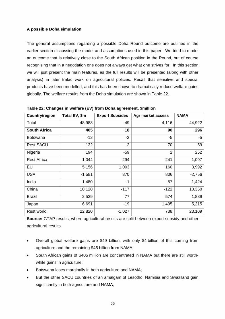
56

A possible Doha simulation

The general assumptions regarding a possible Doha Round outcome are outlined in the

earlier section discussing the model and assumptions used in this paper. We tried to model

an outcome that is relatively close to the South African position in the Round, but of course

recognising that in a negotiation one does not always get what one strives for. In this section

we will just present the main features, as the full results will be presented (along with other

analysis) in later tralac work on agricultural policies. Recall that sensitive and special

products have been modelled, and this has been shown to dramatically reduce welfare gains

globally. The welfare results from the Doha simulation are shown in Table 22.

Table 22: Changes in welfare (EV) from Doha agreement, $million Country/region Total EV, $m Export Subsides Agr market access NAMA

Total 48,988 -49 4,116 44,922

South Africa 405 18 90 296

Botswana -12 -2 -5 -5

Rest SACU 132 2 70 59

Nigeria 194 -59 2 252

Rest Africa 1,044 -294 241 1,097

EU 5,156 1,003 160 3,992

USA -1,581 370 806 -2,756

India 1,480 -1 57 1,424

China 10,120 -117 -122 10,350

Brazil 2,539 77 574 1,889

Japan 6,691 -19 1,495 5,215

Rest world 22,820 -1,027 738 23,109

Source: GTAP results, where agricultural results are split between export subsidy and other

agricultural results.

• Overall global welfare gains are $49 billion, with only $4 billion of this coming from

agriculture and the remaining $45 billion from NAMA;

• South African gains of $405 million are concentrated in NAMA but there are still worth-

while gains in agriculture;

• Botswana loses marginally in both agriculture and NAMA;

• But the other SACU countries of an amalgam of Lesotho, Namibia and Swaziland gain

significantly in both agriculture and NAMA;

57

• The rest of Africa gains overall. The losses in agriculture from the abolition of export

subsidies are balanced by gains from better agricultural market access, and there are

gains from NAMA reforms;

• The EU is a big gainer, with a significant amount of this from the abolition of its own

export subsidies;

• Surprisingly, the USA is an overall loser, with loses in NAMA greater than the gains from

agriculture reform;

• Both India and Brazil are big winners, with most of India’s gains coming from NAMA and

Brazil making significant gains from agricultural reform;

• China is the biggest winner, with large gains in NAMA more than dominating losses in

agriculture;

• Japan is also a significant gainer in both agriculture and NAMA; and

• The rest of the world loses from the abolition of export subsidies but makes large gains

in NAMA to become a clear overall winner.

For South Africa there a production increase in apparel (4.8%), motor vehicles (1.1%) and

the ‘IBSA golden sector’ of other metals of 1.0 percent in industrial goods, and declines of

3.0 percent in sugar production but increases of around three percent in both beef and milk

production in the agricultural sectors. Importantly, in agriculture there is a 29 percent

increase in wheat production, providing evidence that it is hampered by agricultural

distortions elsewhere. For market prices the split is clear: increases for all agricultural

products except beverages and tobacco, but declines for all manufacturing prices.

Post-Doha IBSA analysis

The general welfare changes to IBSA following a modest but successful Doha outcome are

shown below in Table 23. The welfare gains for South Africa are reduced by 11 percent:

from $1,437 billion to $1,279 billion. A cursory analysis of the results shows that the ‘golden

sector’ output still increases but by a lower 13.96 percent (15.5% before) but apparel

production declines by a lesser 6.8 percent (8.7% before) and vehicles are practically

unchanged with a decline of 1.53 percent (1.6% before). From the model we can see that in

agricultural products South Africa is deemed to be sheltering its sensitive/special products of

sugar and milk products in agriculture and textiles/apparel and motor vehicles in the NAMA

sectors.

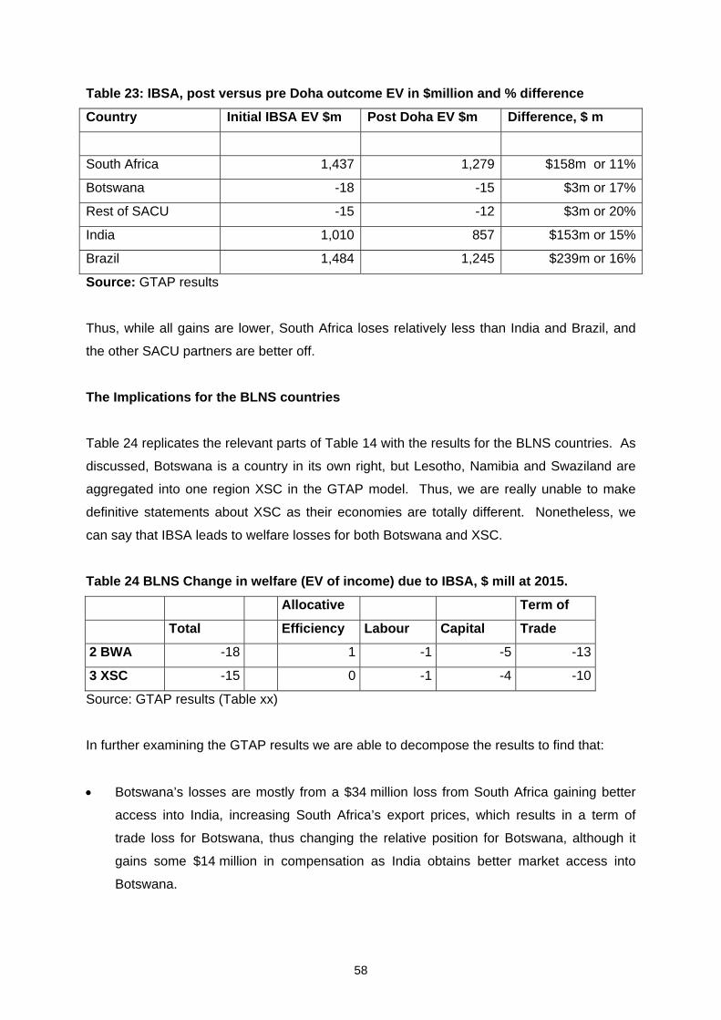
58

Table 23: IBSA, post versus pre Doha outcome EV in $million and % difference

Country Initial IBSA EV $m Post Doha EV $m Difference, $ m

South Africa 1,437 1,279 $158m or 11%

Botswana -18 -15 $3m or 17%

Rest of SACU -15 -12 $3m or 20%

India 1,010 857 $153m or 15%

Brazil 1,484 1,245 $239m or 16%


Thus, while all gains are lower, South Africa loses relatively less than India and Brazil, and

the other SACU partners are better off.

The Implications for the BLNS countries

Table 24 replicates the relevant parts of Table 14 with the results for the BLNS countries. As

discussed, Botswana is a country in its own right, but Lesotho, Namibia and Swaziland are

aggregated into one region XSC in the GTAP model. Thus, we are really unable to make

definitive statements about XSC as their economies are totally different. Nonetheless, we

can say that IBSA leads to welfare losses for both Botswana and XSC.

Table 24 BLNS Change in welfare (EV of income) due to IBSA, $ mill at 2015.

Allocative Term of

Total Efficiency Labour Capital Trade

2 BWA -18 1 -1 -5 -13

3 XSC -15 0 -1 -4 -10

Source: GTAP results (Table xx)

In further examining the GTAP results we are able to decompose the results to find that:

• Botswana’s losses are mostly from a $34 million loss from South Africa gaining better

access into India, increasing South Africa’s export prices, which results in a term of

trade loss for Botswana, thus changing the relative position for Botswana, although it

gains some $14 million in compensation as India obtains better market access into

Botswana.

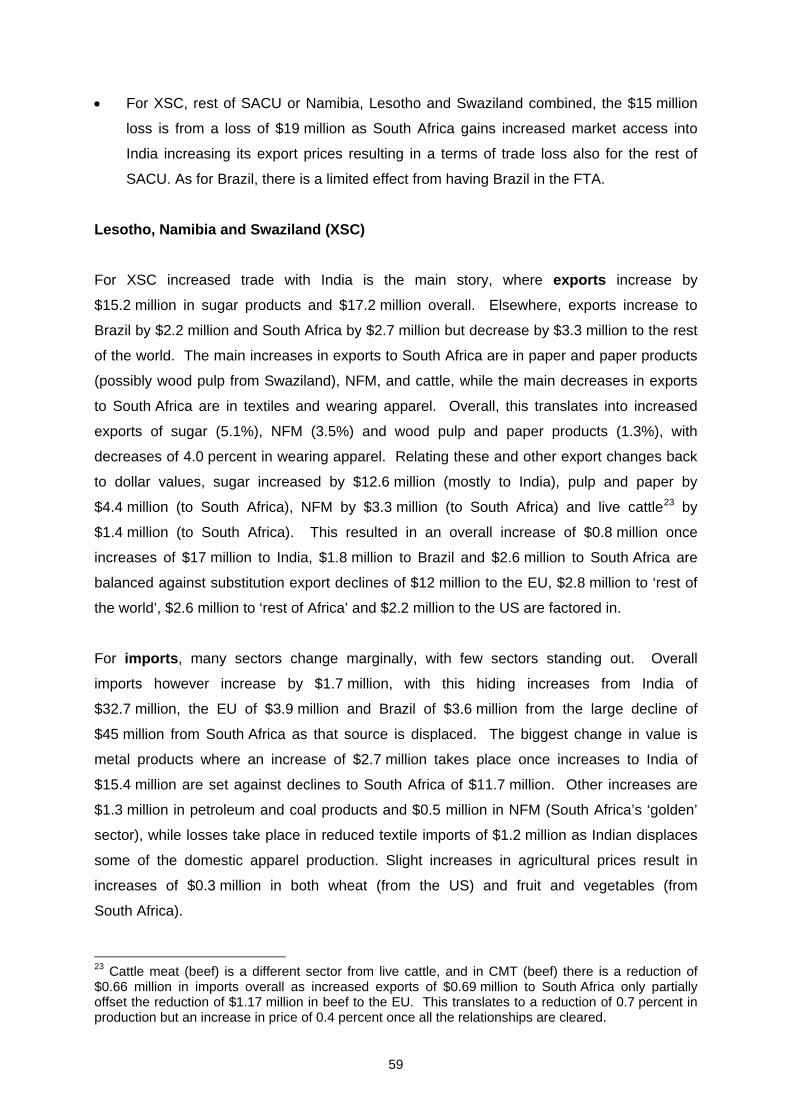
59

• For XSC, rest of SACU or Namibia, Lesotho and Swaziland combined, the $15 million

loss is from a loss of $19 million as South Africa gains increased market access into

India increasing its export prices resulting in a terms of trade loss also for the rest of

SACU. As for Brazil, there is a limited effect from having Brazil in the FTA.

Lesotho, Namibia and Swaziland (XSC)

For XSC increased trade with India is the main story, where exports increase by

$15.2 million in sugar products and $17.2 million overall. Elsewhere, exports increase to

Brazil by $2.2 million and South Africa by $2.7 million but decrease by $3.3 million to the rest

of the world. The main increases in exports to South Africa are in paper and paper products

(possibly wood pulp from Swaziland), NFM, and cattle, while the main decreases in exports

to South Africa are in textiles and wearing apparel. Overall, this translates into increased

exports of sugar (5.1%), NFM (3.5%) and wood pulp and paper products (1.3%), with

decreases of 4.0 percent in wearing apparel. Relating these and other export changes back

to dollar values, sugar increased by $12.6 million (mostly to India), pulp and paper by

$4.4 million (to South Africa), NFM by $3.3 million (to South Africa) and live cattle23 by

$1.4 million (to South Africa). This resulted in an overall increase of $0.8 million once

increases of $17 million to India, $1.8 million to Brazil and $2.6 million to South Africa are

balanced against substitution export declines of $12 million to the EU, $2.8 million to ‘rest of

the world’, $2.6 million to ‘rest of Africa’ and $2.2 million to the US are factored in.

For imports, many sectors change marginally, with few sectors standing out. Overall

imports however increase by $1.7 million, with this hiding increases from India of

$32.7 million, the EU of $3.9 million and Brazil of $3.6 million from the large decline of

$45 million from South Africa as that source is displaced. The biggest change in value is

metal products where an increase of $2.7 million takes place once increases to India of

$15.4 million are set against declines to South Africa of $11.7 million. Other increases are

$1.3 million in petroleum and coal products and $0.5 million in NFM (South Africa’s ‘golden’

sector), while losses take place in reduced textile imports of $1.2 million as Indian displaces

some of the domestic apparel production. Slight increases in agricultural prices result in

increases of $0.3 million in both wheat (from the US) and fruit and vegetables (from

South Africa).

23 Cattle meat (beef) is a different sector from live cattle, and in CMT (beef) there is a reduction of $0.66 million in imports overall as increased exports of $0.69 million to South Africa only partially offset the reduction of $1.17 million in beef to the EU. This translates to a reduction of 0.7 percent in production but an increase in price of 0.4 percent once all the relationships are cleared.

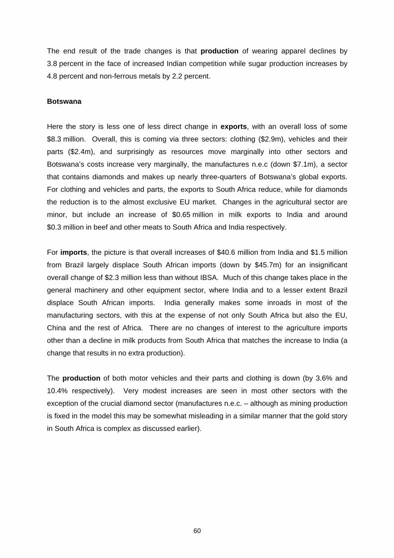
60

The end result of the trade changes is that production of wearing apparel declines by

3.8 percent in the face of increased Indian competition while sugar production increases by

4.8 percent and non-ferrous metals by 2.2 percent.

Botswana

Here the story is less one of less direct change in exports, with an overall loss of some

$8.3 million. Overall, this is coming via three sectors: clothing ($2.9m), vehicles and their

parts ($2.4m), and surprisingly as resources move marginally into other sectors and

Botswana’s costs increase very marginally, the manufactures n.e.c (down $7.1m), a sector

that contains diamonds and makes up nearly three-quarters of Botswana’s global exports.

For clothing and vehicles and parts, the exports to South Africa reduce, while for diamonds

the reduction is to the almost exclusive EU market. Changes in the agricultural sector are

minor, but include an increase of $0.65 million in milk exports to India and around

$0.3 million in beef and other meats to South Africa and India respectively.

For imports, the picture is that overall increases of $40.6 million from India and $1.5 million

from Brazil largely displace South African imports (down by $45.7m) for an insignificant

overall change of $2.3 million less than without IBSA. Much of this change takes place in the

general machinery and other equipment sector, where India and to a lesser extent Brazil

displace South African imports. India generally makes some inroads in most of the

manufacturing sectors, with this at the expense of not only South Africa but also the EU,

China and the rest of Africa. There are no changes of interest to the agriculture imports

other than a decline in milk products from South Africa that matches the increase to India (a

change that results in no extra production).

The production of both motor vehicles and their parts and clothing is down (by 3.6% and

10.4% respectively). Very modest increases are seen in most other sectors with the

exception of the crucial diamond sector (manufactures n.e.c. – although as mining production

is fixed in the model this may be somewhat misleading in a similar manner that the gold story

in South Africa is complex as discussed earlier).

61

References

Bouet, A., Decrex, Y., Fontagne, L., Jean, S. and Laborde, D. 2005. A consistent, ad-

valorem equivalent measure of applied protection across the world: The MAcMap-HS6

database. CEPII No 2004 – 22 December (updated September 2005). [Online]. Available:

http://www.cepii.fr/anglaisgraph/workpap/pdf/2004/wp04-22.pdf.

Dimaranan, B.V. (ed.). 2005. Global trade, Assistance and production: the GTAP 6 Data

Base. Center for Global trade Analysis, Purdue University.

Jensen, H.G. and Sandrey, R. 2006. A possible SACU/China Free Trade Agreement (FTA):

Implications for the South African manufacturing sector. tralac Working Paper 8/2006, July’

Van Meijl, H., Van Rheenen, T., Tabeau, A. and Eickhout, B. 2006. The Impact of different

policy environments on agricultural land use in Europe. Agriculture Ecosystems &

Environment 114 (2006) 21 – 38.

Sandrey, R. 2006a. South African Merchandise Trade with India. tralac Working paper

10/2006, August.

Sandrey, R. 2006b. Trade Creation and Trade Diversion Resulting from SACU trading

Agreements. tralac Working paper 11/2006, August.

Sandrey, R. 2006c. The Trade and Economic Implications of the South African Restrictions

regime on imports of clothing from China. tralac Working Paper 16/2006, October.

Sandrey, R., Matlanyane, A. and Maleleka, D. 2006, Trade Liberalisation: What exactly does

it mean for Lesotho? tralac Working Paper 7/2006, June.

Walmsley, T.L. 2006. A Baseline Scenario for Dynamic GTAP Model’. Revised March 2006

for the GTAP 6 Database. Center for Global Trade Analysis, Purdue University.

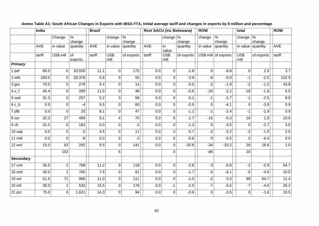
http://www.cepii.fr/anglaisgraph/workpap/pdf/2004/wp04-22.pdf

62

Annex Table A1: South African Changes in Exports with IBSA FTA, Initial average tariff and changes in exports by $ million and percentage India Brazil Rest SACU (inc Botswana) ROW total ROW

Change % change

change % change

change % change

change % change

change % change

AVE in value quantity AVE in value quantity AVE in value

quantity in value quantity in value quantity AVE

tariff US$ mill of exports

tariff US$ mill

of exports tariff US$ mill

of exports US$ mill of exports US$ mill

of exports tariff

Primary

1 pdr 80.0 0 33,559 11.1 0 175 0.0 0 -1.8 0 -9.8 0 2.9 3.7

2 wht 100.0 5 29,376 5.8 0 55 0.0 0 -3.9 -6 -5.9 -1 -2.0 132.9

3 gro 70.0 0 279 5.4 0 14 0.0 0 -0.5 -2 -1.9 -2 -1.5 43.8

4 v_f 45.4 6 289 11.5 0 48 0.0 0 -0.6 -24 -2.2 -18 -1.8 6.5

5 osd 31.3 0 257 5.2 0 58 0.0 0 -0.1 -1 -2.7 -1 -2.5 8.8

6 c_b 0.0 0 -4 9.5 0 60 0.0 0 -0.5 0 -4.1 0 -3.9 0.9

7 pfb 5.0 0 25 8.1 0 47 0.0 0 -1.1 -1 -2.4 -1 -1.9 0.9

8 ocr 32.3 27 459 9.1 4 70 0.0 0 -1.7 -15 -5.3 16 2.9 10.6

9 ctl 31.0 0 182 0.0 0 -2 0.0 0 -1.3 0 -3.5 0 -2.7 3.5

10 oap 0.0 0 -2 4.5 0 11 0.0 0 -0.7 -2 -2.2 -2 -1.9 2.6

11 rmk 0.0 0 -6 0.0 0 -2 0.0 0 -5.6 0 -6.5 0 -6.4 0.0

12 wol 15.0 63 292 9.5 0 141 0.0 0 -20.8 -34 -33.2 29 18.6 1.0

102 5 0 -86 20

Secondary

17 cmt 35.0 2 768 11.2 0 118 0.0 0 -2.8 -3 -5.8 -2 -2.9 54.7

18 omt 30.0 1 765 7.5 0 81 0.0 0 -1.7 -5 -6.1 -5 -4.0 10.5

19 vol 51.6 71 966 11.0 0 111 0.0 0 -1.0 -2 -3.3 69 64.7 11.4

20 mil 30.0 1 533 15.5 0 176 0.0 -1 -2.5 -7 -5.5 -7 -4.0 26.2

21 pcr 75.0 0 1,621 14.3 0 94 0.0 0 -0.6 0 -3.5 0 -1.6 10.5

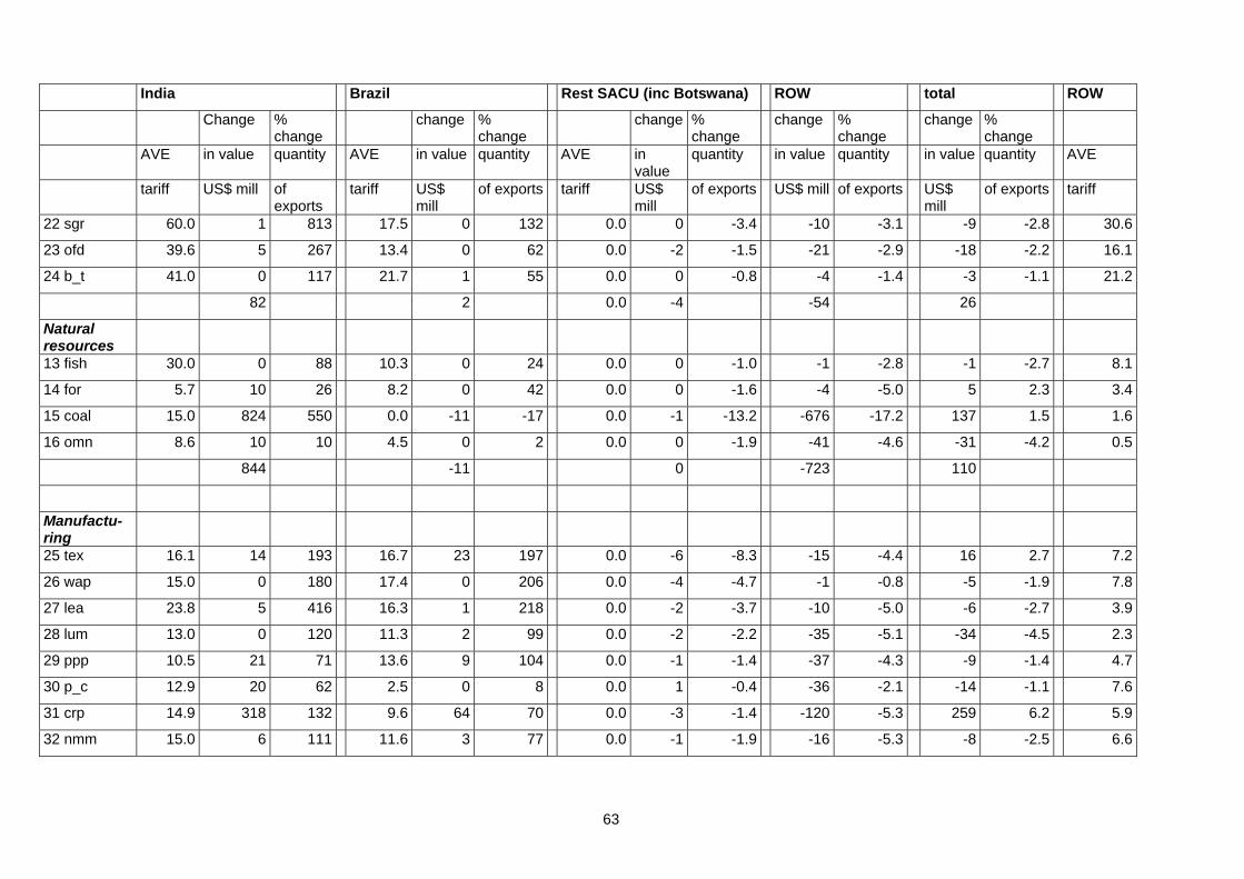
63

India Brazil Rest SACU (inc Botswana) ROW total ROW

Change % change

change % change

change % change

change % change

change % change




tariff US$ mill



of exports tariff

22 sgr 60.0 1 813 17.5 0 132 0.0 0 -3.4 -10 -3.1 -9 -2.8 30.6

23 ofd 39.6 5 267 13.4 0 62 0.0 -2 -1.5 -21 -2.9 -18 -2.2 16.1

24 b_t 41.0 0 117 21.7 1 55 0.0 0 -0.8 -4 -1.4 -3 -1.1 21.2

82 2 0.0 -4 -54 26

Natural resources

13 fish 30.0 0 88 10.3 0 24 0.0 0 -1.0 -1 -2.8 -1 -2.7 8.1

14 for 5.7 10 26 8.2 0 42 0.0 0 -1.6 -4 -5.0 5 2.3 3.4

15 coal 15.0 824 550 0.0 -11 -17 0.0 -1 -13.2 -676 -17.2 137 1.5 1.6

16 omn 8.6 10 10 4.5 0 2 0.0 0 -1.9 -41 -4.6 -31 -4.2 0.5

844 -11 0 -723 110

Manufactu-ring

25 tex 16.1 14 193 16.7 23 197 0.0 -6 -8.3 -15 -4.4 16 2.7 7.2

26 wap 15.0 0 180 17.4 0 206 0.0 -4 -4.7 -1 -0.8 -5 -1.9 7.8

27 lea 23.8 5 416 16.3 1 218 0.0 -2 -3.7 -10 -5.0 -6 -2.7 3.9

28 lum 13.0 0 120 11.3 2 99 0.0 -2 -2.2 -35 -5.1 -34 -4.5 2.3

29 ppp 10.5 21 71 13.6 9 104 0.0 -1 -1.4 -37 -4.3 -9 -1.4 4.7

30 p_c 12.9 20 62 2.5 0 8 0.0 1 -0.4 -36 -2.1 -14 -1.1 7.6

31 crp 14.9 318 132 9.6 64 70 0.0 -3 -1.4 -120 -5.3 259 6.2 5.9

32 nmm 15.0 6 111 11.6 3 77 0.0 -1 -1.9 -16 -5.3 -8 -2.5 6.6

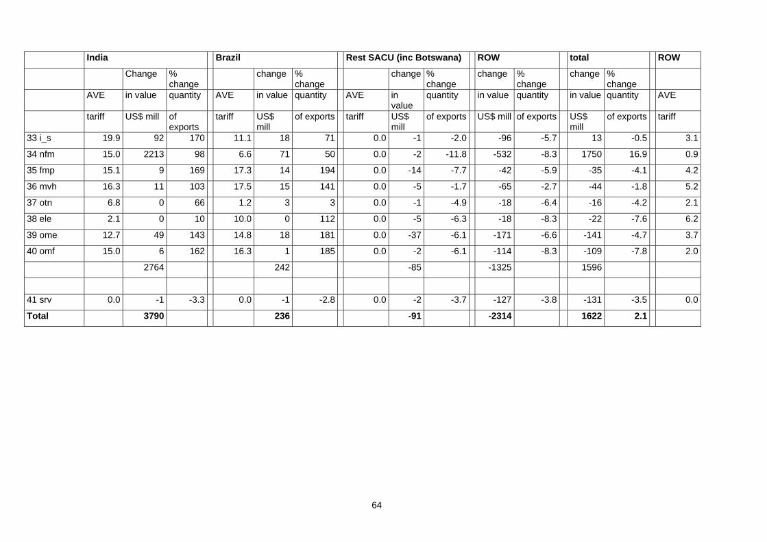
64

India Brazil Rest SACU (inc Botswana) ROW total ROW

Change % change

change % change

change % change

change % change

change % change




tariff US$ mill



of exports tariff

33 i_s 19.9 92 170 11.1 18 71 0.0 -1 -2.0 -96 -5.7 13 -0.5 3.1

34 nfm 15.0 2213 98 6.6 71 50 0.0 -2 -11.8 -532 -8.3 1750 16.9 0.9

35 fmp 15.1 9 169 17.3 14 194 0.0 -14 -7.7 -42 -5.9 -35 -4.1 4.2

36 mvh 16.3 11 103 17.5 15 141 0.0 -5 -1.7 -65 -2.7 -44 -1.8 5.2

37 otn 6.8 0 66 1.2 3 3 0.0 -1 -4.9 -18 -6.4 -16 -4.2 2.1

38 ele 2.1 0 10 10.0 0 112 0.0 -5 -6.3 -18 -8.3 -22 -7.6 6.2

39 ome 12.7 49 143 14.8 18 181 0.0 -37 -6.1 -171 -6.6 -141 -4.7 3.7

40 omf 15.0 6 162 16.3 1 185 0.0 -2 -6.1 -114 -8.3 -109 -7.8 2.0

2764 242 -85 -1325 1596

41 srv 0.0 -1 -3.3 0.0 -1 -2.8 0.0 -2 -3.7 -127 -3.8 -131 -3.5 0.0

Total 3790 236 -91 -2314 1622 2.1

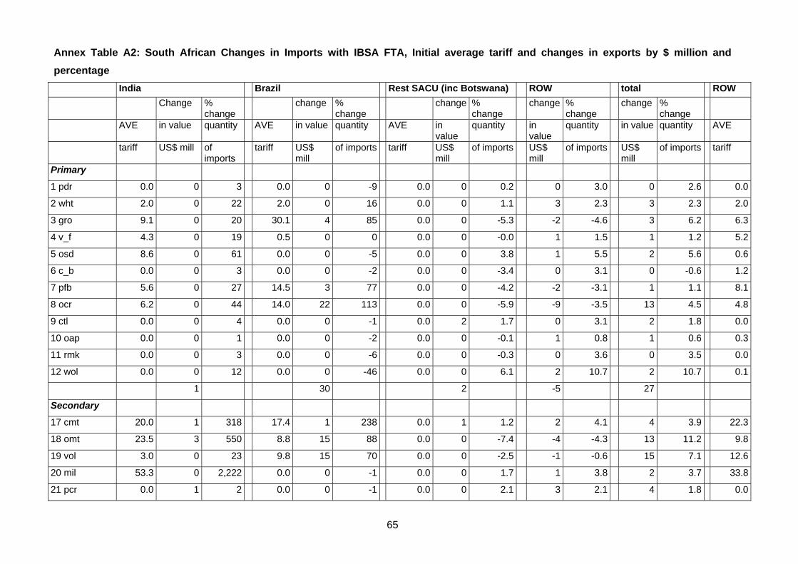
65

Annex Table A2: South African Changes in Imports with IBSA FTA, Initial average tariff and changes in exports by $ million and percentage

India Brazil Rest SACU (inc Botswana) ROW total ROW Change %

change change %

change change %

change change %

change change %

change


quantity in value

quantity in value quantity AVE

tariff US$ mill of imports

tariff US$ mill

of imports tariff US$ mill

of imports US$ mill

of imports US$ mill

of imports tariff

Primary

1 pdr 0.0 0 3 0.0 0 -9 0.0 0 0.2 0 3.0 0 2.6 0.0

2 wht 2.0 0 22 2.0 0 16 0.0 0 1.1 3 2.3 3 2.3 2.0

3 gro 9.1 0 20 30.1 4 85 0.0 0 -5.3 -2 -4.6 3 6.2 6.3

4 v_f 4.3 0 19 0.5 0 0 0.0 0 -0.0 1 1.5 1 1.2 5.2

5 osd 8.6 0 61 0.0 0 -5 0.0 0 3.8 1 5.5 2 5.6 0.6

6 c_b 0.0 0 3 0.0 0 -2 0.0 0 -3.4 0 3.1 0 -0.6 1.2

7 pfb 5.6 0 27 14.5 3 77 0.0 0 -4.2 -2 -3.1 1 1.1 8.1

8 ocr 6.2 0 44 14.0 22 113 0.0 0 -5.9 -9 -3.5 13 4.5 4.8

9 ctl 0.0 0 4 0.0 0 -1 0.0 2 1.7 0 3.1 2 1.8 0.0

10 oap 0.0 0 1 0.0 0 -2 0.0 0 -0.1 1 0.8 1 0.6 0.3

11 rmk 0.0 0 3 0.0 0 -6 0.0 0 -0.3 0 3.6 0 3.5 0.0

12 wol 0.0 0 12 0.0 0 -46 0.0 0 6.1 2 10.7 2 10.7 0.1

1 30 2 -5 27

Secondary

17 cmt 20.0 1 318 17.4 1 238 0.0 1 1.2 2 4.1 4 3.9 22.3

18 omt 23.5 3 550 8.8 15 88 0.0 0 -7.4 -4 -4.3 13 11.2 9.8

19 vol 3.0 0 23 9.8 15 70 0.0 0 -2.5 -1 -0.6 15 7.1 12.6

20 mil 53.3 0 2,222 0.0 0 -1 0.0 0 1.7 1 3.8 2 3.7 33.8

21 pcr 0.0 1 2 0.0 0 -1 0.0 0 2.1 3 2.1 4 1.8 0.0

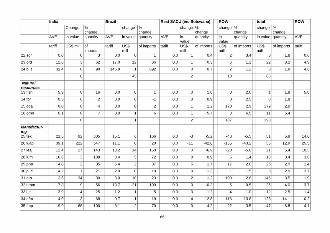
66


change change %

change change %

change change %

change change %

change


quantity in value



tariff US$ mill


of imports US$ mill

of imports US$ mill

of imports tariff

22 sgr 0.0 0 3 0.0 0 1 0.0 1 0.4 2 3.4 3 1.8 0.0

23 ofd 12.6 3 62 17.0 12 86 0.0 1 0.3 6 1.1 22 3.2 4.9

24 b_t 31.4 0 90 145.8 1 692 0.0 0 0.7 2 1.2 3 1.8 4.6

8 45 2 10 66

Natural resources

13 fish 5.9 0 16 0.0 0 1 0.0 0 1.6 0 2.0 1 1.8 5.0

14 for 0.3 0 2 0.0 0 -1 0.0 0 0.9 0 2.5 0 1.8

15 coal 0.0 0 4 0.0 0 2 0.0 1 1.2 178 2.9 179 2.9

16 omn 0.1 0 7 0.0 1 6 0.0 1 5.7 8 6.5 11 6.4

0 1 2 187 190

Manufactur-ing

25 tex 21.5 92 305 15.1 6 166 0.0 -3 -5.2 -43 -5.5 51 5.9 14.6

26 wap 39.1 222 547 11.1 0 20 0.0 -11 -42.8 -155 -43.2 55 12.9 25.5

27 lea 12.4 27 143 13.2 14 150 0.0 0 -6.9 -20 -5.6 21 5.4 10.5

28 lum 16.8 3 188 8.4 5 72 0.0 0 0.9 5 1.4 13 3.4 3.8

29 ppp 4.8 2 35 5.4 2 37 0.0 5 1.7 17 2.8 26 2.9 1.4

30 p_c 4.2 1 21 2.0 0 10 0.0 0 1.3 1 1.5 3 2.9 3.7

31 crp 3.6 34 30 3.0 10 23 0.0 2 1.2 100 2.6 146 3.5 1.9

32 nmm 7.8 9 56 13.7 21 109 0.0 0 -0.3 5 0.5 35 4.0 3.7

33 i_s 3.9 14 25 1.2 1 5 0.0 0 -1.2 -4 -1.0 12 2.5 1.4

34 nfm 4.0 3 68 0.7 1 19 0.0 4 12.8 116 13.8 123 14.1 0.2

35 fmp 9.9 68 100 8.1 2 70 0.0 0 -4.2 -22 -3.5 47 6.8 4.1

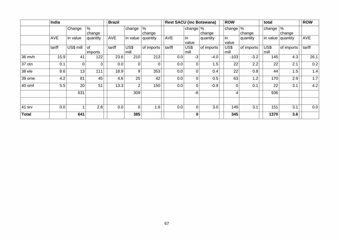
67


change change %

change change %

change change %

change change %

change


quantity in value



tariff US$ mill


of imports US$ mill

of imports US$ mill

of imports tariff

36 mvh 15.9 41 122 23.6 210 213 0.0 -3 -4.0 -103 -3.2 145 4.3 26.1

37 otn 0.1 0 3 0.0 0 0 0.0 0 1.5 22 2.2 22 2.1 0.2

38 ele 8.6 13 111 18.9 9 353 0.0 0 0.4 22 0.8 44 1.5 1.4

39 ome 4.2 81 45 4.6 25 42 0.0 0 0.5 63 1.2 170 2.9 1.7

40 omf 5.5 20 51 13.3 2 150 0.0 0 -0.9 0 0.1 22 3.1 4.2

631 309 -6 4 936

41 srv 0.0 1 2.8 0.0 0 1.6 0.0 0 3.0 149 3.1 151 3.1 0.0

Total 641 385 0 345 1370 3.6

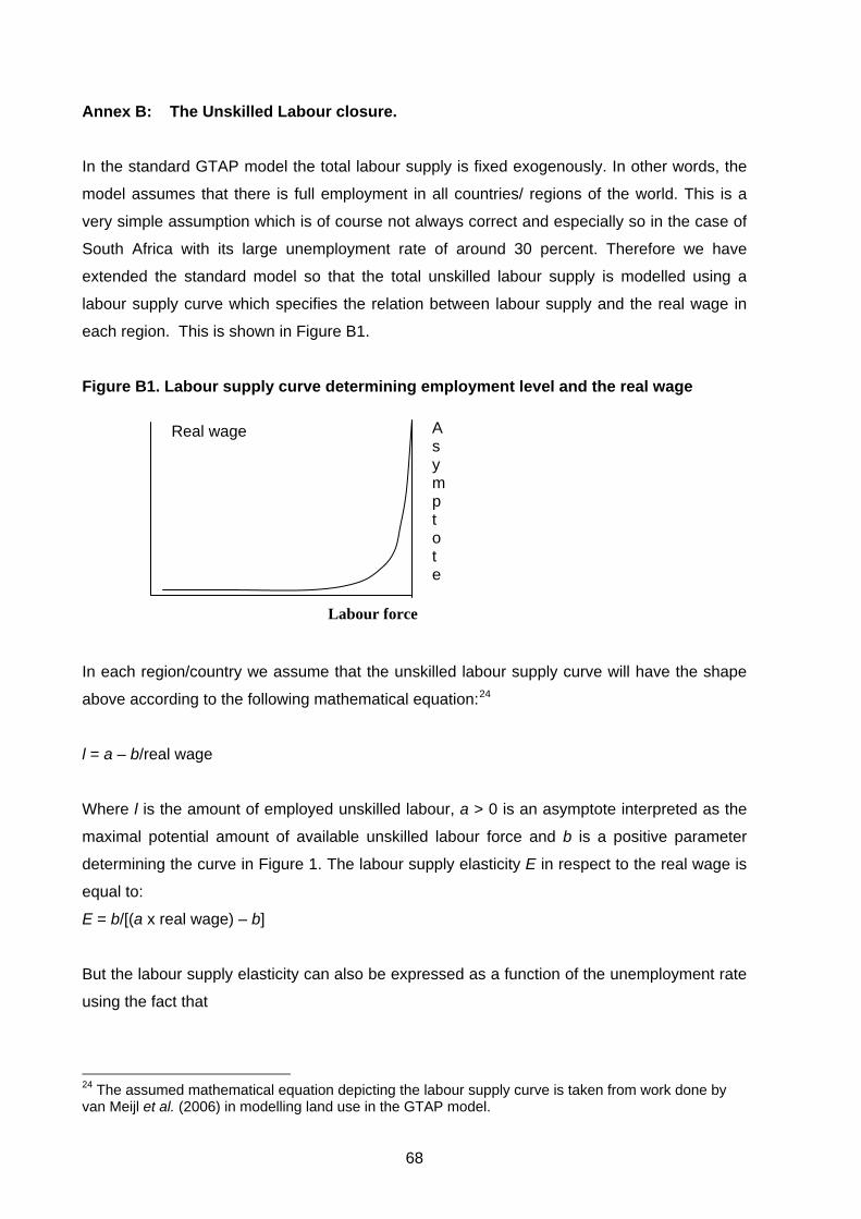
68

Annex B: The Unskilled Labour closure.

In the standard GTAP model the total labour supply is fixed exogenously. In other words, the

model assumes that there is full employment in all countries/ regions of the world. This is a

very simple assumption which is of course not always correct and especially so in the case of

South Africa with its large unemployment rate of around 30 percent. Therefore we have

extended the standard model so that the total unskilled labour supply is modelled using a

labour supply curve which specifies the relation between labour supply and the real wage in

each region. This is shown in Figure B1.

Figure B1. Labour supply curve determining employment level and the real wage

In each region/country we assume that the unskilled labour supply curve will have the shape

above according to the following mathematical equation:24

l = a – b/real wage

Where l is the amount of employed unskilled labour, a > 0 is an asymptote interpreted as the

maximal potential amount of available unskilled labour force and b is a positive parameter

determining the curve in Figure 1. The labour supply elasticity E in respect to the real wage is

equal to:

E = b/[(a x real wage) – b]

But the labour supply elasticity can also be expressed as a function of the unemployment rate

using the fact that

24 The assumed mathematical equation depicting the labour supply curve is taken from work done by van Meijl et al. (2006) in modelling land use in the GTAP model.

Real wage Asympt ot e

Labour force

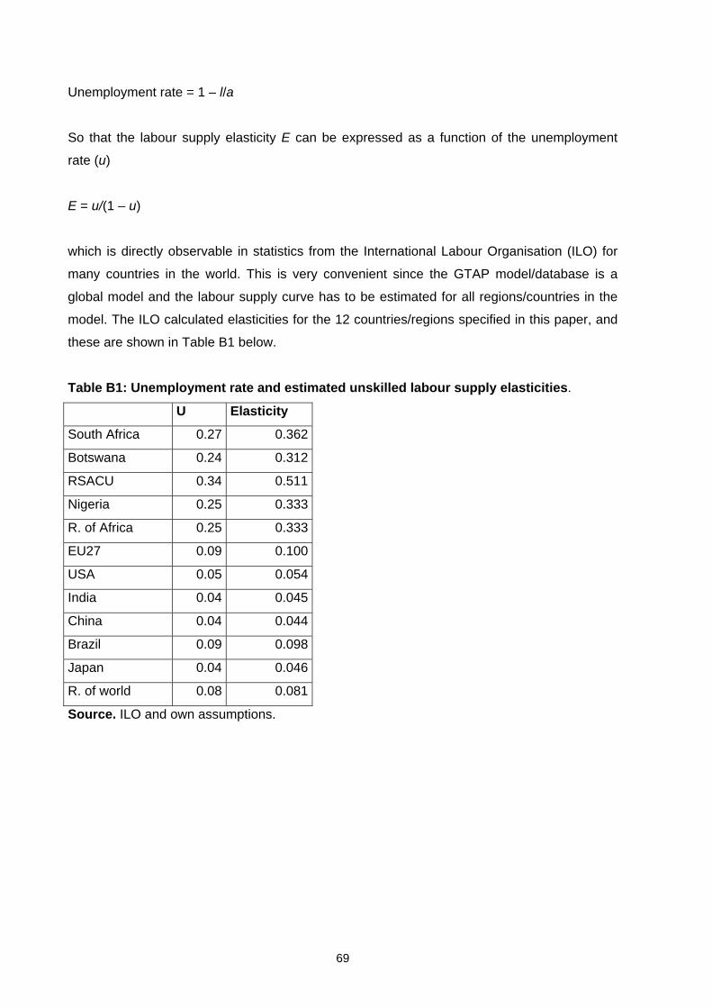
69

Unemployment rate = 1 – l/a

So that the labour supply elasticity E can be expressed as a function of the unemployment

rate (u)

E = u/(1 – u)

which is directly observable in statistics from the International Labour Organisation (ILO) for

many countries in the world. This is very convenient since the GTAP model/database is a

global model and the labour supply curve has to be estimated for all regions/countries in the

model. The ILO calculated elasticities for the 12 countries/regions specified in this paper, and

these are shown in Table B1 below.

Table B1: Unemployment rate and estimated unskilled labour supply elasticities.

U Elasticity

South Africa 0.27 0.362

Botswana 0.24 0.312

RSACU 0.34 0.511

Nigeria 0.25 0.333

R. of Africa 0.25 0.333

EU27 0.09 0.100

USA 0.05 0.054

India 0.04 0.045

China 0.04 0.044

Brazil 0.09 0.098

Japan 0.04 0.046

R. of world 0.08 0.081

Source. ILO and own assumptions.

Documents

Global Trade Analysis Project (GTAP) - Examining the India, Brazil … · 2007-08-28 · 1 Summary and general conclusions from the analysis Following a comprehensive examination