Embed Size (px)
Citation preview
1chap
ter
international monetary Fund | October 2013 1
1chap
ter
Global growth is still weak, its underlying dynam-ics are changing, and the risks to the forecast remain to the downside. As a result, new policy challenges are arising and policy spillovers may pose greater concern. In particular, markets are increasingly convinced that U.S. monetary policy is reaching a turning point, and this has led to an unexpectedly large increase in long-term yields in the United States and many other economies, notwithstanding the Federal Reserve’s recent decision to maintain its asset purchases. This change could pose risks for emerging market economies, where activity is slowing and asset quality weakening. Careful policy implementation and clear communication on the part of the Federal Reserve will be essential. Also, growth in China is slowing, which will affect many other economies, notably the commodity exporters among the emerging market and developing economies. At the same time, old problems––a fragmented financial system in the euro area and worrisomely high public debt in all major advanced economies––remain unresolved and could trigger new crises. The major economies must urgently adopt policies that improve their prospects; otherwise the global economy may well settle into a subdued medium-term growth trajectory. The United States and Japan must develop and implement strong plans with concrete measures for medium-term fiscal adjustment and entitle-ment reform, and the euro area must develop a stronger currency union and clean up its financial systems. China should provide a permanent boost to private consump-tion spending to rebalance the growth of demand away from exports and investment. Many emerging market economies need a new round of structural reforms.
Growth Dynamics Further DivergeGlobal growth remains in low gear, averaging only 2½ percent during the fi rst half of 2013, which is about the same pace as in the second half of 2012. In a departure from previous developments since the Great Recession, the advanced economies have recently gained some speed, while the emerging market econo-
mies have slowed (Figure 1.1, panel 1). Th e emerging market economies, however, continue to account for the bulk of global growth. Within each group, there are still broad diff erences in growth and position in the cycle.
Th e latest indicators point to somewhat better pros-pects in the near term but diff erent growth dynamics between the major economies (Figure 1.2). World Eco-nomic Outlook (WEO) projections continue to foresee a modest acceleration of activity, driven largely by the advanced economies (Table 1.1). • The impulse to global growth is expected to come
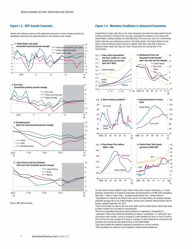
mainly from the United States (Figure 1.3, panel 1), where activity will move into higher gear as fiscal consolidation eases and monetary conditions stay supportive. Following sharp fiscal tighten-ing earlier this year, activity in the United States is already regaining speed, helped by a recovering real estate sector (Figure 1.4, panel 5), higher household wealth, easier bank lending conditions (Figure 1.4, panel 3), and more borrowing (Figure 1.4, panels 2 and 4). The fiscal tightening in 2013 is estimated to be 2½ percent of GDP (Table A8 in the Statistical Appendix). However, this will ease to ¾ percent of GDP in 2014, helping raise the rate of economic growth to 2½ percent, from 1½ percent in 2013 (see Table 1.1). This assumes that discretionary pub-lic spending is authorized and executed as projected and the debt ceiling is raised in a timely manner.
• In Japan, activity is projected to slow in response to tightening fiscal policy in 2014. Thus far, the data point to an impressive pickup in output in response to the Bank of Japan’s Quantitative and Qualitative Monetary Easing and the government’s 1.4 percent of GDP fiscal stimulus to end deflation and raise growth. IMF staff estimates suggest that the new policies may have boosted GDP by about 1 percent, although wage increases have remained subdued. As stimulus and reconstruction spending unwind and consumption tax hikes are implemented, the structural deficit will drop––the projections assume a decline by 2½ percent of GDP in 2014, which
GLOBaL prOSpectS aND pOLIcIeS
world economic outlook: transitions and tensions
2 international monetary Fund | October 2013
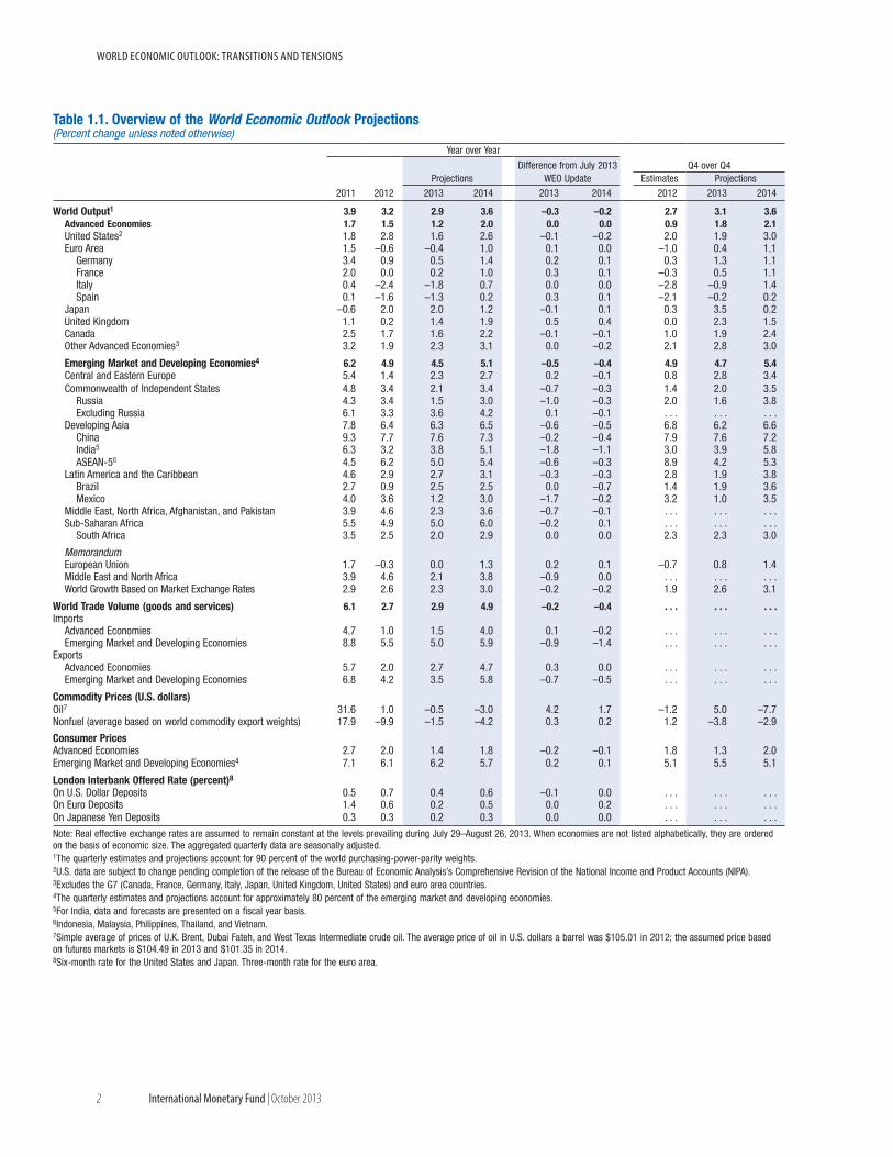
Table 1.1. Overview of the World Economic Outlook Projections(Percent change unless noted otherwise)
Year over Year
Difference from July 2013 WEO Update
Q4 over Q4Projections Estimates Projections
2011 2012 2013 2014 2013 2014 2012 2013 2014
World Output1 3.9 3.2 2.9 3.6 –0.3 –0.2 2.7 3.1 3.6Advanced Economies 1.7 1.5 1.2 2.0 0.0 0.0 0.9 1.8 2.1United States2 1.8 2.8 1.6 2.6 –0.1 –0.2 2.0 1.9 3.0Euro Area 1.5 –0.6 –0.4 1.0 0.1 0.0 –1.0 0.4 1.1
Germany 3.4 0.9 0.5 1.4 0.2 0.1 0.3 1.3 1.1France 2.0 0.0 0.2 1.0 0.3 0.1 –0.3 0.5 1.1Italy 0.4 –2.4 –1.8 0.7 0.0 0.0 –2.8 –0.9 1.4Spain 0.1 –1.6 –1.3 0.2 0.3 0.1 –2.1 –0.2 0.2
Japan –0.6 2.0 2.0 1.2 –0.1 0.1 0.3 3.5 0.2United Kingdom 1.1 0.2 1.4 1.9 0.5 0.4 0.0 2.3 1.5Canada 2.5 1.7 1.6 2.2 –0.1 –0.1 1.0 1.9 2.4Other Advanced Economies3 3.2 1.9 2.3 3.1 0.0 –0.2 2.1 2.8 3.0
Emerging Market and Developing Economies4 6.2 4.9 4.5 5.1 –0.5 –0.4 4.9 4.7 5.4Central and Eastern Europe 5.4 1.4 2.3 2.7 0.2 –0.1 0.8 2.8 3.4Commonwealth of Independent States 4.8 3.4 2.1 3.4 –0.7 –0.3 1.4 2.0 3.5
Russia 4.3 3.4 1.5 3.0 –1.0 –0.3 2.0 1.6 3.8Excluding Russia 6.1 3.3 3.6 4.2 0.1 –0.1 . . . . . . . . .
Developing Asia 7.8 6.4 6.3 6.5 –0.6 –0.5 6.8 6.2 6.6China 9.3 7.7 7.6 7.3 –0.2 –0.4 7.9 7.6 7.2India5 6.3 3.2 3.8 5.1 –1.8 –1.1 3.0 3.9 5.8ASEAN-56 4.5 6.2 5.0 5.4 –0.6 –0.3 8.9 4.2 5.3
Latin America and the Caribbean 4.6 2.9 2.7 3.1 –0.3 –0.3 2.8 1.9 3.8Brazil 2.7 0.9 2.5 2.5 0.0 –0.7 1.4 1.9 3.6Mexico 4.0 3.6 1.2 3.0 –1.7 –0.2 3.2 1.0 3.5
Middle East, North Africa, Afghanistan, and Pakistan 3.9 4.6 2.3 3.6 –0.7 –0.1 . . . . . . . . .Sub-Saharan Africa 5.5 4.9 5.0 6.0 –0.2 0.1 . . . . . . . . .
South Africa 3.5 2.5 2.0 2.9 0.0 0.0 2.3 2.3 3.0
Memorandum European Union 1.7 –0.3 0.0 1.3 0.2 0.1 –0.7 0.8 1.4Middle East and North Africa 3.9 4.6 2.1 3.8 –0.9 0.0 . . . . . . . . .World Growth Based on Market Exchange Rates 2.9 2.6 2.3 3.0 –0.2 –0.2 1.9 2.6 3.1
World Trade Volume (goods and services) 6.1 2.7 2.9 4.9 –0.2 –0.4 . . . . . . . . .Imports
Advanced Economies 4.7 1.0 1.5 4.0 0.1 –0.2 . . . . . . . . .Emerging Market and Developing Economies 8.8 5.5 5.0 5.9 –0.9 –1.4 . . . . . . . . .
ExportsAdvanced Economies 5.7 2.0 2.7 4.7 0.3 0.0 . . . . . . . . .Emerging Market and Developing Economies 6.8 4.2 3.5 5.8 –0.7 –0.5 . . . . . . . . .
Commodity Prices (U.S. dollars)Oil7 31.6 1.0 –0.5 –3.0 4.2 1.7 –1.2 5.0 –7.7Nonfuel (average based on world commodity export weights) 17.9 –9.9 –1.5 –4.2 0.3 0.2 1.2 –3.8 –2.9
Consumer PricesAdvanced Economies 2.7 2.0 1.4 1.8 –0.2 –0.1 1.8 1.3 2.0Emerging Market and Developing Economies4 7.1 6.1 6.2 5.7 0.2 0.1 5.1 5.5 5.1
London Interbank Offered Rate (percent)8
On U.S. Dollar Deposits 0.5 0.7 0.4 0.6 –0.1 0.0 . . . . . . . . .On Euro Deposits 1.4 0.6 0.2 0.5 0.0 0.2 . . . . . . . . .On Japanese Yen Deposits 0.3 0.3 0.2 0.3 0.0 0.0 . . . . . . . . .
Note: Real effective exchange rates are assumed to remain constant at the levels prevailing during July 29–August 26, 2013. When economies are not listed alphabetically, they are ordered on the basis of economic size. The aggregated quarterly data are seasonally adjusted.1The quarterly estimates and projections account for 90 percent of the world purchasing-power-parity weights.2U.S. data are subject to change pending completion of the release of the Bureau of Economic Analysis’s Comprehensive Revision of the National Income and Product Accounts (NIPA).3Excludes the G7 (Canada, France, Germany, Italy, Japan, United Kingdom, United States) and euro area countries.4The quarterly estimates and projections account for approximately 80 percent of the emerging market and developing economies. 5For India, data and forecasts are presented on a fiscal year basis.6Indonesia, Malaysia, Philippines, Thailand, and Vietnam.7Simple average of prices of U.K. Brent, Dubai Fateh, and West Texas Intermediate crude oil. The average price of oil in U.S. dollars a barrel was $105.01 in 2012; the assumed price based on futures markets is $104.49 in 2013 and $101.35 in 2014.8Six-month rate for the United States and Japan. Three-month rate for the euro area.
c h a p t e r 1 G lo b a l P r o s P e c ts a n d P o l i c i e s
international monetary Fund | October 2013 3
Figure 1.1. Global Growth
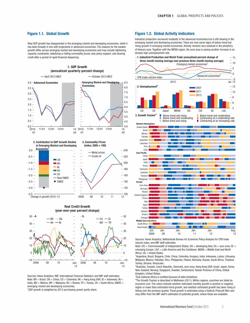
Real GDP growth has disappointed in the emerging market and developing economies, while ithas been broadly in line with projections in advanced economies. The reasons for the weakergrowth differ across emerging market and developing economies and may include tightening capacity constraints, stabilizing or falling commodity prices, less policy support, and slowing credit after a period of rapid financial deepening.
–10
0
10
20
30
40
50
2006 08 10 Jun.13
BR CNHK IN
Real Credit Growth(year-over-year percent change)
4.
–10
0
10
20
30
40
50
2006 08 10 Jun.13
5.CO IDMY TR
April 2013 WEO October 2013 WEO
0.0
0.5
1.0
1.5
2.0
2.5
3.0
3.5
4.0
2010:H1
11:H1 12:H1 13:H1 14:H2
Advanced Economies
4.0
4.5
5.0
5.5
6.0
6.5
7.0
7.5
8.0
8.5
2010:H1
11:H1 12:H1 13:H1 14:H2
Emerging Market and Developing Economies
1. GDP Growth(annualized quarterly percent change)
100
120
140
160
180
200
220
240
2008 09 10 11 12
3. Commodity Prices (index; 2005 = 100)
–3.5
–3.0
–2.5
–2.0
–1.5
–1.0
–0.5
0.0
Change in growth 2010–13
2. Contribution to GDP Growth Decline in Emerging Market and Developing Economies1
Metal pricesCrude oil
CNBRINRUZARest EMDEEMDE
Sources: Haver Analytics; IMF, International Financial Statistics; and IMF staff estimates.Note: BR = Brazil; CN = China; CO = Colombia; HK = Hong Kong SAR; ID = Indonesia; IN = India; MX = Mexico; MY = Malaysia; RU = Russia; TR = Turkey; ZA = South Africa; EMDE = emerging market and developing economies.1GDP growth is weighted by 2013 purchasing-power-parity share.
Western HemisphereUnited States
Brazil
MexicoCanada
Argentina
ColombiaPeru
ChileAsia Pacific
China
JapanIndia
Korea
Indonesia
Australia
Thailand
PhilippinesEurope
Euro Area
GermanyRussia
United KingdomFrance
Italy
SpainTurkey
SwedenGreece
PortugalMiddle East and Africa
South Africa
Saudi Arabia
3
6
9
12
15
US EA Japan MENA DA CIS EE LAC
3. Growth Tracker4
–5
0
5
10
15
2012 Jul. 13
Figure 1.2. Global Activity Indicators Industrial production recovered modestly in the advanced economies but is still slowing in the emerging market and developing economies. There are now some signs of below-trend but rising growth in emerging market economies. Activity remains very subdued in the periphery of theeuro area. Together with the MENA region, the euro area is seeing another increase in an already high unemployment rate.
1. Industrial Production and World Trade (annualized percent change of three-month moving average over previous three-month moving average)
2. Unemployment3
Above trend and moderating
Jun.2008
Jan.09
Jan.10
Jan.11
Aug.13
Above trend and rising Below trend and moderatingContracting at a moderating rateContracting at an increasing rate
Jan.12
Below trend and rising
200720112013
Advanced economies2
Emerging market economies1
CPB trade volume index
Sources: Haver Analytics; Netherlands Bureau for Economic Policy Analysis for CPB trade volume index; and IMF staff estimates.Note: CIS = Commonwealth of Independent States; DA = developing Asia; EA = euro area; EE = emerging Europe; LAC = Latin America and the Caribbean; MENA = Middle East and North Africa; US = United States.1Argentina, Brazil, Bulgaria, Chile, China, Colombia, Hungary, India, Indonesia, Latvia, Lithuania, Malaysia, Mexico, Pakistan, Peru, Philippines, Poland, Romania, Russia, South Africa, Thailand, Turkey, Ukraine, Venezuela.2Australia, Canada, Czech Republic, Denmark, euro area, Hong Kong SAR, Israel, Japan, Korea, New Zealand, Norway, Singapore, Sweden, Switzerland, Taiwan Province of China, United Kingdom, United States.3Sub-Saharan Africa is omitted because of data limitations.4The Growth Tracker is described in Matheson (2011). Within regions, countries are listed by economic size. The colors indicate whether estimated monthly growth is positive or negative, higher or lower than estimated trend growth, and whether estimated growth has been rising or falling over the previous quarter. Trend growth is estimated using a Hodrick-Prescott filter and may differ from the IMF staff’s estimates of potential growth, where these are available.
world economic outlook: transitions and tensions
4 international monetary Fund | October 2013
–2
0
2
4
6
8
10
2010:H1
11:H1 12:H1 13:H1 14:H2
0
2
4
6
8
10
12
14
2010:H1
11:H1 12:H1 13:H1 14:H2
Figure 1.3. GDP Growth Forecasts
Activity will continue to pick up in the advanced economies. In many emerging market and developing economies, the projected pickup is now relatively more modest.
–4
–2
0
2
4
6
8
2010 11 12 13
–3–2–10123456
–9–6–30369121518
2010 11 12 13 14:Q4
1. United States and Japan(annualized quarterly percent change)
2. Euro Area(annualized quarterly percent change)
Source: IMF staff estimates.
3. Developing Asia (half-over-half annualized percent change)
4. Latin America and the Caribbean (half-over-half annualized percent change)
Advanced economies (left scale)United States (left scale)Japan (right scale)
Euro areaFrance and GermanySpain and Italy
ChinaIndiaDeveloping Asia
Latin AmericaBrazilMexico
14:Q4
90
100
110
120
130
140
150
2000 02 04 06 08 10 13:Q2
0
5
10
15
20
25
30
35
40
45
2007 08 09 10 11 12 Sep.13
Figure 1.4. Monetary Conditions in Advanced Economies
Expectations for policy rate hikes in the major advanced economies have been pulled forward.Lending continues to contract in the euro area, especially the periphery, but is rising in the United States. Lending conditions are still tightening in the euro area, even if to a diminishing extent, while they are continuing to loosen in the United States. The Federal Reserve’s and Bank of Japan’s balance sheets continue to expand, while that of the ECB contracts as periphery banks repay their long-term loans. House prices are coming back in the United States.
–40
–20
0
20
40
60
80
100
2000 02 04 06 08 10 13:Q3
3. Bank Lending Conditions3
–10
–5
0
5
10
15
20
2006 07 08 09 10 11 12 13:Q2
2. Nonfinancial Firm andHousehold Credit Growth2
(year-over-year percent change)
0.0
0.1
0.2
0.3
0.4
0.5
0.6
0.7
0.8
0.9
t t + 12 t + 24 t + 36
1. Policy Rate Expectations1
(percent; months on x-axis;dashed lines are from theApril 2013 WEO)
5. Real House Price Indices (2000 = 100)
6. Central Bank Total Assets (percent of 2008 GDP)
70
80
90
100
110
120
130
140
2000 02 04 06 08 10 13:Q1
4. Household Debt-to-Income Ratio
United StatesEuro areaSpainItaly
United States
Euro area United States
Euro area4
United States
Euro area
Fed
ECB5
BOJ
United Kingdom
United States
Europe
Sources: Bank of America/Merrill Lynch; Bank of Italy; Bank of Spain; Bloomberg, L.P.; Haver Analytics; Organization for Economic Cooperation and Development; and IMF staff calculations.Note: BOJ = Bank of Japan; ECB = European Central Bank; Fed = Federal Reserve.1Expectations are based on the federal funds rate for the United States, the sterling overnight interbank average rate for the United Kingdom, and the euro interbank offered forward rate for Europe; updated September 24, 2013.2Flow of funds data are used for the euro area, Spain, and the United States. Italian bank loans to Italian residents are corrected for securitizations.3Percent of respondents describing lending standards as tightening “considerably”or “somewhat” minus those indicating standards are easing “considerably” or “somewhat” over the previous three months. Survey of changes to credit standards for loans or lines of credit to firms for the euro area; average of surveys on changes in credit standards for commercial and industrial and commercial real estate lending for the United States.4Euro area includes the subsector employers (including own-account workers).5ECB calculations are based on the Eurosystem’s weekly financial statement.
c h a p t e r 1 G lo b a l P r o s P e c ts a n d P o l i c i e s
international monetary Fund | October 2013 5
is expected to drag down growth from 2 percent in 2013 to 1¼ percent in 2014. However, if another “stimulus package” does go ahead, fiscal drag would be lower and growth higher than presently projected.
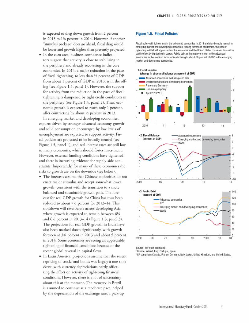
• In the euro area, business confidence indica-tors suggest that activity is close to stabilizing in the periphery and already recovering in the core economies. In 2014, a major reduction in the pace of fiscal tightening, to less than ½ percent of GDP from about 1 percent of GDP in 2013, is in the off-ing (see Figure 1.5, panel 1). However, the support for activity from the reduction in the pace of fiscal tightening is dampened by tight credit conditions in the periphery (see Figure 1.4, panel 2). Thus, eco-nomic growth is expected to reach only 1 percent, after contracting by about ½ percent in 2013.In emerging market and developing economies,
exports driven by stronger advanced economy growth and solid consumption encouraged by low levels of unemployment are expected to support activity. Fis-cal policies are projected to be broadly neutral (see Figure 1.5, panel 1), and real interest rates are still low in many economies, which should foster investment. However, external funding conditions have tightened and there is increasing evidence for supply-side con-straints. Importantly, for many of these economies the risks to growth are on the downside (see below). • The forecasts assume that Chinese authorities do not
enact major stimulus and accept somewhat lower growth, consistent with the transition to a more balanced and sustainable growth path. The fore-cast for real GDP growth for China has thus been reduced to about 7½ percent for 2013–14. This slowdown will reverberate across developing Asia, where growth is expected to remain between 6¼ and 6½ percent in 2013–14 (Figure 1.3, panel 3). The projections for real GDP growth in India have also been marked down significantly, with growth foreseen at 3¾ percent in 2013 and about 5 percent in 2014. Some economies are seeing an appreciable tightening of financial conditions because of the recent global reversal in capital flows.
• In Latin America, projections assume that the recent repricing of stocks and bonds was largely a one-time event, with currency depreciations partly offset-ting the effect on activity of tightening financial conditions. However, there is a lot of uncertainty about this at the moment. The recovery in Brazil is assumed to continue at a moderate pace, helped by the depreciation of the exchange rate, a pick-up
–1
0
1
2
3
2010 11 12 13 14
–10
–8
–6
–4
–2
0
2
4
2001 05 09 13 18
0
20
40
60
80
100
120
140
1950 60 70 80 90 2000 10 18
Source: IMF staff estimates.1Greece, Ireland, Italy, Portugal, Spain.2G7 comprises Canada, France, Germany, Italy, Japan, United Kingdom, and United States.
Figure 1.5. Fiscal Policies
Fiscal policy will tighten less in the advanced economies in 2014 and stay broadly neutral in emerging market and developing economies. Among advanced economies, the pace of tightening will fall off appreciably in the euro area and the United States. However, this will be partly offset by tightening in Japan. Public debt will remain very high in the advanced economies in the medium term, while declining to about 30 percent of GDP in the emerging market and developing economies.
2. Fiscal Balance(percent of GDP)
3. Public Debt(percent of GDP)
1. Fiscal Impulse(change in structural balance as percent of GDP)
Advanced economies excluding euro areaEmerging market and developing economiesFrance and GermanyEuro area periphery1
April 2013 WEO
Advanced economiesEmerging market and developing economiesWorld
Advanced economiesG72
Emerging market and developing economiesWorld
world economic outlook: transitions and tensions
6 international monetary Fund | October 2013
in consumption, and policies aimed at boosting investment. Mexico will receive a fillip from the rebound in U.S. activity, following a disappointing first half in 2013. The acceleration of activity across the continent, however, will be modest (Figure 1.3, panel 4).
• In sub-Saharan Africa, commodity-related projects are expected to support higher growth. Exchange rates adjusted sharply, but external financing has resumed and the forecasts include no further disruptions.
• In the Middle East, North Africa, Afghanistan, and Pakistan activity is projected to accelerate in 2014, supported by a modest recovery in oil production. Non-oil activity will remain generally robust in the oil-exporting economies, thanks in part to high public spending. By contrast, many oil-importing economies continue to struggle with difficult socio-political and security conditions.
• In central and eastern Europe, growth rates are projected to gradually increase, helped by recovering demand in Europe and improving domestic finan-cial conditions. With a few exceptions, the effects of externally induced increases in interest rates will be limited and partly offset by currency depreciations. Many economies of the Commonwealth of Indepen-dent States are still seeing strong domestic demand; they will benefit from more external demand, although some will suffer from the recent external funding shocks.
Inflation pressure Is Subdued
The differing growth dynamics between the major economies are projected to come with subdued infla-tion pressure, for two reasons. First, the pickup in activity in the advanced economies will not lead to a major reduction in output gaps, which remain large (see Table A8 in the Statistical Appendix). Second, commodity prices have fallen amid improved supply and lower demand growth from key emerging market economies, notably China (see the Special Feature). The latest projections for both fuel and nonfuel prices indicate modest declines in both 2013 and 2014.
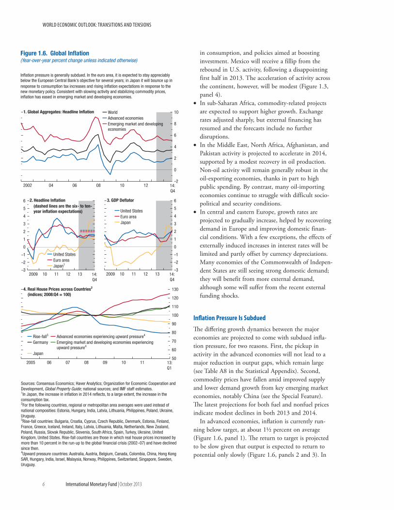
In advanced economies, inflation is currently run-ning below target, at about 1½ percent on average (Figure 1.6, panel 1). The return to target is projected to be slow given that output is expected to return to potential only slowly (Figure 1.6, panels 2 and 3). In
50
60
70
80
90
100
110
120
130
2005 06 07 08 09 10 11 13:Q1
–3
–2
–1
0
1
2
3
4
5
6
2009 10 11 12 13 14:Q4
Figure 1.6. Global Inflation(Year-over-year percent change unless indicated otherwise)
Inflation pressure is generally subdued. In the euro area, it is expected to stay appreciably below the European Central Bank’s objective for several years; in Japan it will bounce up in response to consumption tax increases and rising inflation expectations in response to the new monetary policy. Consistent with slowing activity and stabilizing commodity prices, inflation has eased in emerging market and developing economies.
–2
0
2
4
6
8
10
2002 04 06 08 10 12 14:Q4
1. Global Aggregates: Headline Inflation
4. Real House Prices across Countries2
(indices; 2008:Q4 = 100)
–3
–2
–1
0
1
2
3
4
5
6
2009 10 11 12 13 14:Q4
3. GDP Deflator
WorldAdvanced economiesEmerging market and developing economies
United StatesEuro areaJapan1
2. Headline Inflation(dashed lines are the six- to ten-year inflation expectations) United States
Euro areaJapan
Rise-fall3 Advanced economies experiencing upward pressure4
Germany Emerging market and developing economies experiencing upward pressure4
Japan
Sources: Consensus Economics; Haver Analytics; Organization for Economic Cooperation and Development, Global Property Guide; national sources; and IMF staff estimates.1In Japan, the increase in inflation in 2014 reflects, to a large extent, the increase in the consumption tax.2For the following countries, regional or metropolitan area averages were used instead of national composities: Estonia, Hungary, India, Latvia, Lithuania, Philippines, Poland, Ukraine, Uruguay.3Rise-fall countries: Bulgaria, Croatia, Cyprus, Czech Republic, Denmark, Estonia, Finland, France, Greece, Iceland, Ireland, Italy, Latvia, Lithuania, Malta, Netherlands, New Zealand, Poland, Russia, Slovak Republic, Slovenia, South Africa, Spain, Turkey, Ukraine, United Kingdom, United States. Rise-fall countries are those in which real house prices increased by more than 10 percent in the run-up to the global financial crisis (2002–07) and have declined since then.4Upward pressure countries: Australia, Austria, Belgium, Canada, Colombia, China, Hong Kong SAR, Hungary, India, Israel, Malaysia, Norway, Philippines, Switzerland, Singapore, Sweden, Uruguay.
c h a p t e r 1 G lo b a l P r o s P e c ts a n d P o l i c i e s
international monetary Fund | October 2013 7
the United States, the decline in the unemployment rate partly reflects reductions in labor force participa-tion due to demographic trends as well as discouraged workers dropping out of the labor force. Discouraged workers are likely to return to the labor market as prospects improve, and thus wage growth will be slug-gish for some time. In the euro area, a weak economy and downward pressure on wages in the periphery are forecast to hold inflation to about 1½ percent in the medium term, falling short of the European Central Bank’s (ECB’s) inflation objective. For Japan, the projection reflects a temporary surge in the price level in response to the consumption tax hikes in 2014 and 2015; excluding the effect of the consumption tax hike, inflation is projected to move up only very gradually, reaching the 2 percent target sometime in 2016–17.
Inflation is expected to move broadly sideways at around 5-6 percent in emerging market and devel-oping economies (Figure 1.6, panel 1). The drop in commodity prices and the downshift in growth will reduce price pressures, but capacity constraints and the pass-through from weakening exchange rates will offset this downward pressure to some degree. Another counterpush to lower inflation will be strong domes-tic demand pressure in a few of these economies––as evidenced by many external overheating indicators that still flash yellow or red (Figure 1.7).
Monetary policies are Gradually Moving in Different Directions
Monetary conditions have stayed supportive glob-ally, although they will increasingly start to reflect the changing growth dynamics in the major economies. Growing uncertainty about the implications for future policies has prompted financial markets to anticipate a greater degree of U.S. monetary policy tightening than in recent WEO forecasts, and this has caused larger-than-expected spillovers on emerging market economies.
The April 2013 WEO argued that “markets may have moved ahead of the real economy” but judged that near-term financial risks had eased. Since then, perceptions have changed in two important respects: • There is strengthening conviction in markets that
U.S. monetary policy will soon reach a turning point. Following the midyear policy meetings of the Federal Reserve and communication hinting
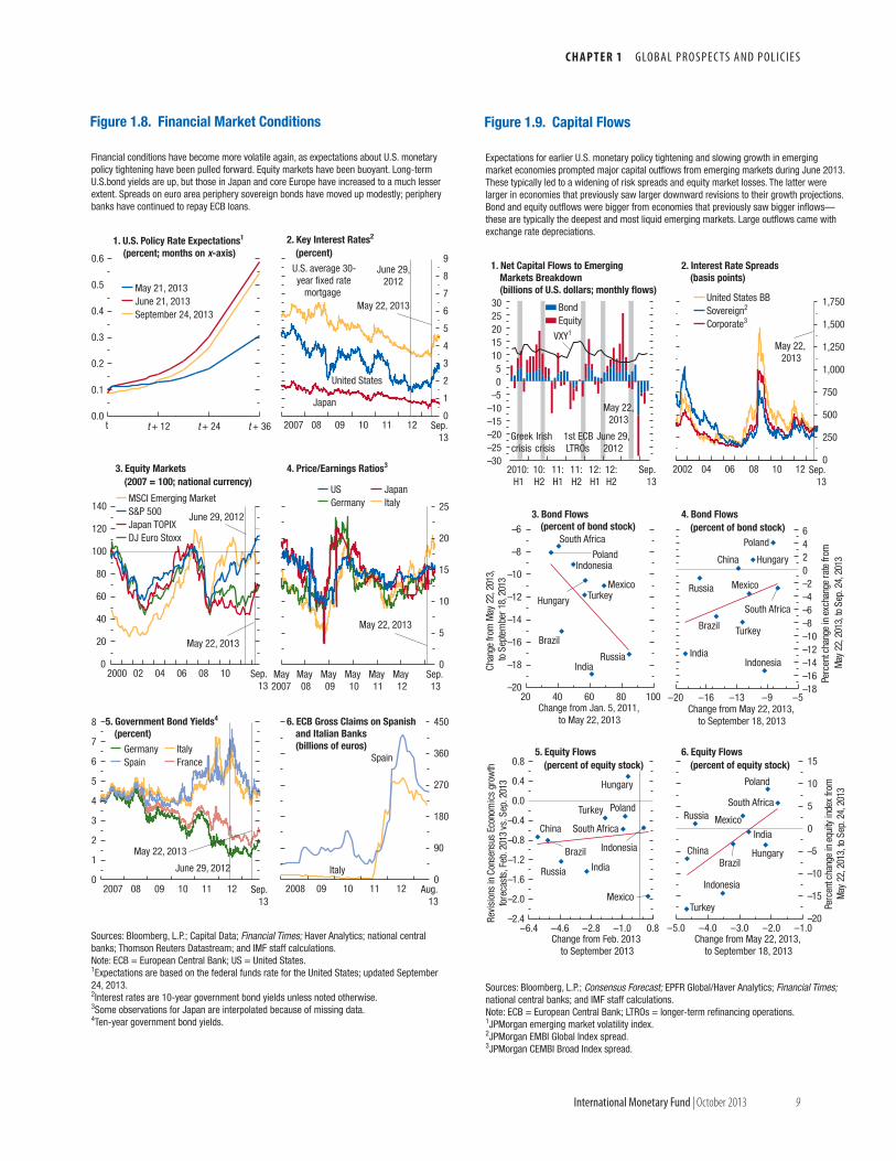
at tapering of asset purchases, market participants raised their expectations for the policy rate (see Fig-ure 1.8, panel 1). Contrary to expectations of many in the markets, however, the Federal Reserve decided not to begin tapering in September. This brought the yield curve down modestly. Nonetheless, since end May 2013, long-term bond yields are up some 100 basis points, as are fixed rates on 30-year mort-gages (see Figure 1.8, panel 2).
• In China, the authorities have attempted to rein in the flow of credit, including through shadow banks, preferring more targeted and limited support (such as to small businesses) over widespread stimulus. These actions are consistent with their intention to move to a more balanced and sustainable growth path. Reflecting this, and the second quarter out-turn, projections for growth this year have been marked down from 7¾ to 7½ percent. Financial conditions have tightened globally in
response to the rise in U.S. long-term bond yields (see Figure 1.8, panels 2 and 5)—spillovers that are not unusual from a historical perspective (Box 1.1).
In the euro area, perceptions of earlier-than-expected U.S. tightening led to asset price losses. Subsequent developments brought about rallies—notably an ECB statement that it expects policy rates to remain at cur-rent levels or lower for an extended period because of a weak economy. Japanese long-term bond yields are up modestly owing to foreign as well as domestic factors.
In emerging markets, the spillovers interacted with weaker growth prospects and rising vulnerabilities. Capital outflows led to a significant tightening of financial conditions for some economies over the sum-mer (Figure 1.9, panel 1). Markdowns to projections for Chinese growth and imports, notably commodities, have added to the repricing. Sovereign bond yields are up some 80 basis points since the beginning of 2013, pulled up by fairly large increases in Brazil, Indonesia, Mexico, South Africa, and Turkey. Equity markets have been retreating to varying degrees, with the larg-est corrections typically in those economies with the largest downward revisions to growth forecasts and the largest recent inflows of capital (Figure 1.9, panels 5 and 6)––so far this year, they are down some 10 per-cent (see Figure 1.8, panel 3). Indicators of equity market volatility are up modestly as are risk spreads (Figure 1.9, panel 2). Capital outflows typically led to currency depreciations (Figure 1.10, panels 1 and 2). The specific developments are discussed in more detail
world economic outlook: transitions and tensions
8 international monetary Fund | October 2013
Output relative to
trend1Output gap
Unemp-loyment Inflation2 Summary
Terms of trade
Capital inflows3
Current account Summary
Credit growth4
House price4
Share price4 Summary
Fiscal Balance5
Real Interest Rate6
Advanced EconomiesJapan
Canada
Germany
United States
France
Australia
Korea
United Kingdom
Italy
Emerging Market and Developing Economies
Indonesia
India
Brazil
Turkey
Argentina7
Saudi Arabia
Russia
China
Mexico
South Africa
Greater than or equal to 0.5 but less than 1.5 standard deviations
Less than 0.5 standard deviation
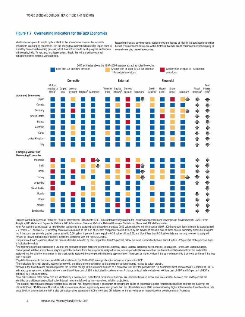
Figure 1.7. Overheating Indicators for the G20 Economies
Most indicators point to ample cyclical slack in the advanced economies but capacity constraints in emerging economies. The red and yellow external indicators for Japan point toa healthy demand-rebalancing process, which has not yet made much progress in Germany. In Indonesia, India, Turkey, and, to a lesser extent, Brazil, the red and yellow external indicators point to external vulnerabilities.
Greater than or equal to 1.5 standard deviations
Financial
2013 estimates above the 1997–2006 average, except as noted below, by:
Domestic External
Sources: Australian Bureau of Statistics; Bank for International Settlements; CEIC China Database; Organization for Economic Cooperation and Development; Global Property Guide; Haver Analytics; IMF, Balance of Payments Statistics; IMF, International Financial Statistics; National Bureau of Statistics of China; and IMF staff estimates.Note: For each indicator, except as noted below, economies are assigned colors based on projected 2013 values relative to their precrisis (1997–2006) average. Each indicator is scored as red = 2, yellow = 1, and blue = 0; summary scores are calculated as the sum of selected component scores divided by the maximum possible sum of those scores. Summary blocks are assigned red if the summary score is greater than or equal to 0.66, yellow if greater than or equal to 0.33 but less than 0.66, and blue if less than 0.33. When data are missing, no color is assigned. Arrows up (down) indicate hotter (colder) conditions compared with the April 2013 WEO.1Output more than 2.5 percent above the precrisis trend is indicated by red. Output less than 2.5 percent below the trend is indicated by blue. Output within ±2.5 percent of the precrisis trend is indicated by yellow.2The following scoring methodology is used for the following inflation-targeting economies: Australia, Brazil, Canada, Indonesia, Korea, Mexico, South Africa, Turkey, and United Kingdom. End-of-period inflation above the country’s target inflation band from the midpoint is assigned yellow; end-of-period inflation more than two times the inflation band from the midpoint is assigned red. For all other economies in the chart, red is assigned if end-of-period inflation is approximately 10 percent or higher, yellow if it is approximately 5 to 9 percent, and blue if it is less than 5 percent.3Capital inflows refer to the latest available value relative to the 1997–2006 average of capital inflows as a percent of GDP.4The indicators for credit growth, house price growth, and share price growth refer to the annual percentage change relative to output growth.5Arrows in the fiscal balance column represent the forecast change in the structural balance as a percent of GDP over the period 2012–13. An improvement of more than 0.5 percent of GDP is indicated by an up arrow; a deterioration of more than 0.5 percent of GDP is indicated by a down arrow. A change in fiscal balance between –0.5 percent of GDP and 0.5 percent of GDP is indicated by a sideways arrow.6Real policy interest rates below zero are identified by a down arrow; real interest rates above 3 percent are identified by an up arrow; real interest rates between zero and 3 percent are identified by a sideways arrow. Real policy interest rates are deflated by two-year-ahead inflation projections.7The data for Argentina are officially reported data. The IMF has, however, issued a declaration of censure and called on Argentina to adopt remedial measures to address the quality of the official GDP and CPI-GBA data. Alternative data sources have shown significantly lower real growth than the official data since 2008 and considerably higher inflation rates than the official data since 2007. In this context, the IMF is also using alternative estimates of GDP growth and CPI inflation for the surveillance of macroeconomic developments in Argentina.
Regarding financial developments, equity prices are flagged as high in the advanced economies but other valuation indicators are within historical bounds. Credit continues to expand rapidly in several emerging market economies.
c h a p t e r 1 G lo b a l P r o s P e c ts a n d P o l i c i e s
international monetary Fund | October 2013 9
Figure 1.8. Financial Market Conditions
0
5
10
15
20
25
May2007
May08
May09
May10
May11
May12
Sep.13
4. Price/Earnings Ratios3
0
20
40
60
80
100
120
140
2000 02 04 06 08 10 Sep.13
3. Equity Markets(2007 = 100; national currency)
June 29, 2012
0
90
180
270
360
450
2008 09 10 11 12 Aug.13
6. ECB Gross Claims on Spanishand Italian Banks(billions of euros)
0
1
2
3
4
5
6
7
8
2007 08 09 10 11 12 Sep.13
5. Government Bond Yields4
(percent)
June 29, 2012
MSCI Emerging MarketS&P 500Japan TOPIXDJ Euro Stoxx
US JapanGermany Italy
Germany ItalySpain France
0
1
2
3
4
5
6
7
8
9
2007 08 09 10 11 12 Sep.13
2. Key Interest Rates2
(percent)
June 29, 2012
Spain
Italy
Japan
United States
May 22, 2013
May 22, 2013
May 22, 2013
May 22, 2013
0.0
0.1
0.2
0.3
0.4
0.5
0.6
t t + 12 t + 24 t + 36
1. U.S. Policy Rate Expectations1
(percent; months on x-axis)
May 21, 2013June 21, 2013September 24, 2013
U.S. average 30-year fixed rate
mortgage
Financial conditions have become more volatile again, as expectations about U.S. monetary policy tightening have been pulled forward. Equity markets have been buoyant. Long-term U.S.bond yields are up, but those in Japan and core Europe have increased to a much lesser extent. Spreads on euro area periphery sovereign bonds have moved up modestly; periphery banks have continued to repay ECB loans.
Sources: Bloomberg, L.P.; Capital Data; Financial Times; Haver Analytics; national central banks; Thomson Reuters Datastream; and IMF staff calculations.Note: ECB = European Central Bank; US = United States.1Expectations are based on the federal funds rate for the United States; updated September 24, 2013.2Interest rates are 10-year government bond yields unless noted otherwise.3Some observations for Japan are interpolated because of missing data.4Ten-year government bond yields.
–20
–18
–16
–14
–12
–10
–8
–6
20 40 60 80 100
South Africa
Mexico
Brazil
Turkey
Russia
Poland
Hungary
Indonesia
IndiaChan
gefro
mM
ay22
,201
3,to
Sept
embe
r18,
2013
Change from Jan. 5, 2011, to May 22, 2013
–2.4
–2.0
–1.6
–1.2
–0.8
–0.4
0.0
0.4
0.8
–6.4 –4.6 –2.8 –1.0 0.8
South Africa
Mexico
Brazil
Turkey
Russia
Poland
Hungary
Indonesia
India
China
Revi
sion
sin
Cons
ensu
sEc
onom
ics
grow
thfo
reca
sts,
Feb.
2013
vs.S
ep.2
013
Change from Feb. 2013 to September 2013
–18–16–14–12–10–8–6–4–20246
–20 –16 –13 –9 –5
South Africa
Mexico
Brazil Turkey
Russia
Poland
Hungary
IndonesiaIndia
China
Perc
entc
hang
ein
exch
ange
rate
from
May
22,2
013,
toSe
p.24
,201
3
Change from May 22, 2013, to September 18, 2013
5. Equity Flows(percent of equity stock)
4. Bond Flows(percent of bond stock)
0
250
500
750
1,000
1,250
1,500
1,750
2002 04 06 08 10 12 Sep.13
Figure 1.9. Capital Flows
2. Interest Rate Spreads(basis points)
Greek crisis
Irish crisis
1st ECBLTROs
United States BBSovereign2
Corporate3
1. Net Capital Flows to Emerging Markets Breakdown (billions of U.S. dollars; monthly flows)
May 22, 2013
June 29, 2012
3. Bond Flows(percent of bond stock)
–20
–15
–10
–5
0
5
10
15
–5.0 –4.0 –3.0 –2.0 –1.0
South Africa
Mexico
Brazil
Turkey
Russia
Poland
Hungary
Indonesia
India
China
Perc
entc
hang
ein
equi
tyin
dex
from
May
22,2
013,
toSe
p.24
,201
3
Change from May 22, 2013, to September 18, 2013
6. Equity Flows(percent of equity stock)
BondEquity
VXY1
May 22, 2013
–30–25–20–15–10–505
1015202530
2010:H1
10:H2
11:H1
11:H2
12:H1
12:H2
Sep.13
Expectations for earlier U.S. monetary policy tightening and slowing growth in emerging market economies prompted major capital outflows from emerging markets during June 2013. These typically led to a widening of risk spreads and equity market losses. The latter were larger in economies that previously saw larger downward revisions to their growth projections. Bond and equity outflows were bigger from economies that previously saw bigger inflows––these are typically the deepest and most liquid emerging markets. Large outflows came with exchange rate depreciations.
Sources: Bloomberg, L.P.; Consensus Forecast; EPFR Global/Haver Analytics; Financial Times; national central banks; and IMF staff calculations.Note: ECB = European Central Bank; LTROs = longer-term refinancing operations.1JPMorgan emerging market volatility index.2JPMorgan EMBI Global Index spread.3JPMorgan CEMBI Broad Index spread.
world economic outlook: transitions and tensions
10 international monetary Fund | October 2013
in the October 2013 Global Financial Stability Report (GFSR).
The WEO projections assume that the recent repric-ing of emerging market bonds and equities was largely a one-time event but there is a lot of uncertainty about this at the moment. The resulting tighter external financial conditions and lower net capital inflow levels should reduce activity in emerging market economies, all else equal.
Model-based estimates suggest that in most of the major emerging market economies the externally induced tightening since late May 2013, should it persist, could reduce GDP by ¼ to 1 percent (Fig-ure 1.11). However, exchange rate depreciation can do much to buffer externally induced tightening. Further considerations include the following: • Although the U.S. recovery is set to acceler-
ate, based of the Federal Reserve’s forward guid-ance, WEO projections continue to assume that the first U.S. policy rate hike will not take place before 2016. The reasons are that inflation is fore-cast to remain below 2½ percent, inflation expecta-tions to stay well anchored, and the unemployment rate to remain above 6½ percent until then. The forecasts assume that Federal Reserve asset purchases are scaled back very gradually starting later this year. The effect of the purchases on activity was widely estimated to have been limited, and their termina-tion is not expected to have a major effect. Accord-ingly, the projected path for longer-term government bond yields in 2014 has been raised modestly, by some 40 basis points relative to the April 2013 WEO. In short, the assumptions are for U.S. mon-etary and financial conditions to generate a benign, growth-friendly environment. Markets, however, see a significant probability of earlier tightening (see Figure 1.8, panel 1), and, as discussed below, a less benign trajectory for financial conditions is a distinct risk.
• Markets continue to expect a prolonged period of low interest rates and unconventional monetary sup-port for the euro area and Japan (Figure 1.4, panel 1). In Japan, further monetary easing may be needed to drive up inflation (excluding consumption tax hikes) to 2 percent by 2015. In the euro area, the dominant concern is still sluggish activity and low inflation, including disinflation or deflation pressure in the periphery. The projections assume no material changes to sovereign spreads in the periphery. They
Figure 1.10. Exchange Rates and Reserves
0
200
400
600
800
1,000
1,200
1,400
1,600
2000 02 04 06 08 10 12 Aug.13
3. International Reserves (index; 2000 = 100, three-month moving average)
Developing AsiaMiddle East and North AfricaEmerging EuropeLatin America and the Caribbean
–20
–15
–10
–5
0
5
10
15
20
Sur. Def. Aln. DEU MYS CHN EA JPN RUS IND IDN US BRA TUR ZAF ESP
Percent change from Jan. 2013 to Aug. 2013Percent change from April 2013 to Aug. 2013
1. Real Effective Exchange Rates (percent change from January 2010 to August 2013)1
–16–14–12–10–8–6–4–20246
Sur. Def. Aln. MYS CHN EA JPN RUS IND IDN BRA TUR ZAF
2. Nominal Exchange Rates (U.S. dollars per national currency; percent change from January 1, 2013, to September 23, 2013)1
Percent change from May 22, 2013, to September 23, 2013
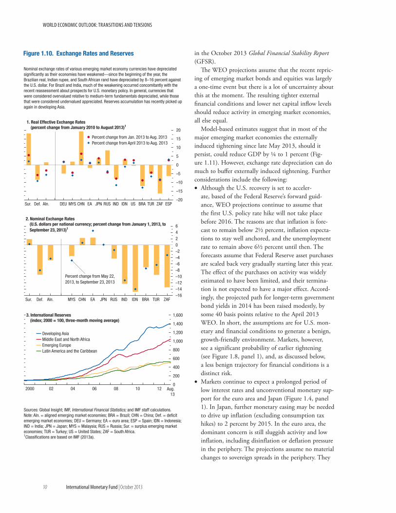
Nominal exchange rates of various emerging market economy currencies have depreciated significantly as their economies have weakened––since the beginning of the year, the Brazilian real, Indian rupee, and South African rand have depreciated by 8–16 percent against the U.S. dollar. For Brazil and India, much of the weakening occurred concomitantly with the recent reassessment about prospects for U.S. monetary policy. In general, currencies that were considered overvalued relative to medium-term fundamentals depreciated, while those that were considered undervalued appreciated. Reserves accumulation has recently picked up again in developing Asia.
Sources: Global Insight; IMF, International Financial Statistics; and IMF staff calculations.Note: Aln. = aligned emerging market economies; BRA = Brazil; CHN = China; Def. = deficit emerging market economies; DEU = Germany; EA = euro area; ESP = Spain; IDN = Indonesia; IND = India; JPN = Japan; MYS = Malaysia; RUS = Russia; Sur. = surplus emerging market economies; TUR = Turkey; US = United States; ZAF = South Africa.1Classifications are based on IMF (2013a).
c h a p t e r 1 G lo b a l P r o s P e c ts a n d P o l i c i e s
international monetary Fund | October 2013 11
also assume that some tightening of credit condi-tions will continue (see Figure 1.4, panel 3). The major factor is banks’ concerns about the economic environment and their need to improve their bal-ance sheets.
Medium-term prospects for emerging Market economies are Weaker
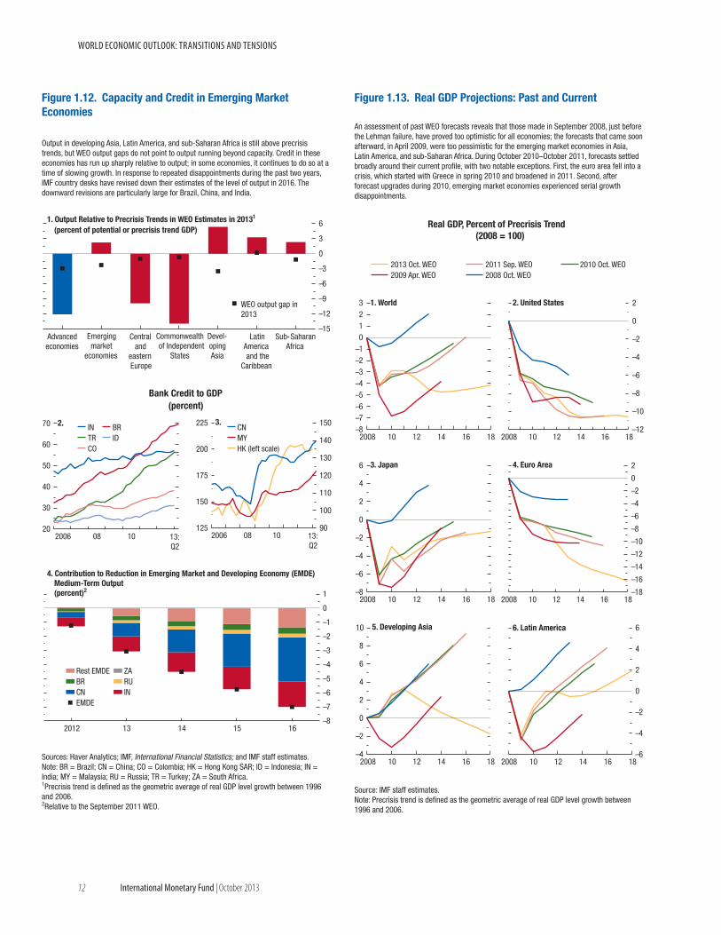
Emerging market and developing economy growth rates are now down some 3 percentage points from 2010 levels, with Brazil, China, and India accounting for about two-thirds of the decline (see Fig-ure 1.1, panel 2). Together with recent forecast disap-pointments, this growth decline has prompted further downgrades to medium-term output projections for emerging market economies. Projections for 2016 real GDP levels for Brazil, China, and India have been successively reduced by some 8 to 14 percent over the past two years. Together, the downward revisions for these three economies account for about three-quarters of the overall reduction in projections for medium-term output for the emerging market and developing economies as a group (Figure 1.12, panel 4).
Postcrisis WEO projections typically assumed that the emerging market and developing economies of Latin America and Asia would avoid the large, permanent out-put losses that were predicted for the crisis-hit econo-mies (Figure 1.13). The pessimistic April 2009 WEO projections, made in the wake of the Lehman Brothers collapse, were repeatedly upgraded for these economies (Figure 1.13, panels 5 and 6). Subsequently, however, the projections were revised downward. Among the other regions, large downgrades materialized only in the euro area periphery as it fell into crisis (Figure 1.13, panel 4). Thus, it seems that domestic factors have played a major role in the slowdown of the emerging market and developing economies. The specific reasons for lower growth differ, and clear diagnoses are hard to obtain. IMF staff analysis suggests that cyclical and structural factors are at play. This seems to be the case for Brazil, India, China, and South Africa (Box 1.2). • Following the Great Recession, most of these
economies enjoyed vigorous, cyclical rebounds. Expansionary macroeconomic policies helped buffer the loss of demand from the advanced economies. Financial factors amplified the cyclical rebound from the recession. In China, credit policy was used deliberately to inject stimulus in the face of flag-
–3
–2
–1
0
1
TR ID BR CN IN RU MX
1. Real GDP(percent deviation)
–15
–10
–5
0
5
TR ID BR CN IN RU MX
2. Bilateral Exchange Rate(against the U.S. dollar; percent deviation; positive = appreciation)
–15
–10
–5
0
5
10
TR ID BR CN IN RU MX
4. Equity Prices(percent deviation)
0
1
2
3
TR ID BR CN IN RU MX
3. Market Interest Rate(percentage point deviation)
–2
0
2
4
6
8
10
12
BR CL CN CO ID IN KR MX MY PE PH PL RU TH TR ZA
5. Real Policy Rates(percent; deflated by two-year-ahead inflation projections)
April 2008 August 2013April 2008 average August 2013 average
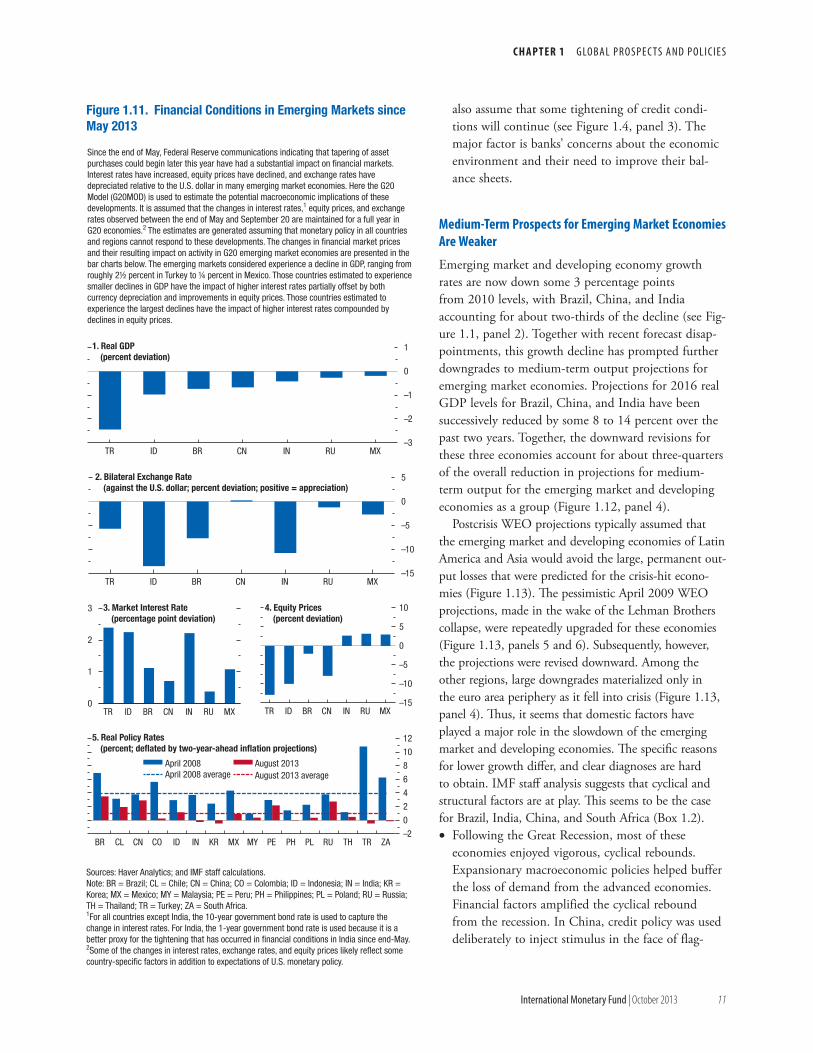
Since the end of May, Federal Reserve communications indicating that tapering of asset purchases could begin later this year have had a substantial impact on financial markets. Interest rates have increased, equity prices have declined, and exchange rates have depreciated relative to the U.S. dollar in many emerging market economies. Here the G20 Model (G20MOD) is used to estimate the potential macroeconomic implications of these developments. It is assumed that the changes in interest rates,1 equity prices, and exchange rates observed between the end of May and September 20 are maintained for a full year in G20 economies.2 The estimates are generated assuming that monetary policy in all countries and regions cannot respond to these developments. The changes in financial market prices and their resulting impact on activity in G20 emerging market economies are presented in the bar charts below. The emerging markets considered experience a decline in GDP, ranging from roughly 2½ percent in Turkey to ¼ percent in Mexico. Those countries estimated to experience smaller declines in GDP have the impact of higher interest rates partially offset by both currency depreciation and improvements in equity prices. Those countries estimated to experience the largest declines have the impact of higher interest rates compounded by declines in equity prices.
Figure 1.11. Financial Conditions in Emerging Markets since May 2013
Sources: Haver Analytics; and IMF staff calculations.Note: BR = Brazil; CL = Chile; CN = China; CO = Colombia; ID = Indonesia; IN = India; KR = Korea; MX = Mexico; MY = Malaysia; PE = Peru; PH = Philippines; PL = Poland; RU = Russia; TH = Thailand; TR = Turkey; ZA = South Africa.1For all countries except India, the 10-year government bond rate is used to capture the change in interest rates. For India, the 1-year government bond rate is used because it is a better proxy for the tightening that has occurred in financial conditions in India since end-May.2Some of the changes in interest rates, exchange rates, and equity prices likely reflect some country-specific factors in addition to expectations of U.S. monetary policy.
world economic outlook: transitions and tensions
12 international monetary Fund | October 2013
125
150
175
200
225
90
100
110
120
130
140
150
2006 08 10 13:Q2
20
30
40
50
60
70
2006 08 10 13:Q2
Figure 1.12. Capacity and Credit in Emerging Market Economies
–15
–12
–9
–6
–3
0
3
6
Advancedeconomies
Emergingmarket
economies
Centraland
easternEurope
Commonwealthof Independent
States
Devel-opingAsia
LatinAmericaand the
Caribbean
Sub-SaharanAfrica
1. Output Relative to Precrisis Trends in WEO Estimates in 20131
(percent of potential or precrisis trend GDP)
IN BRTR IDCO
Bank Credit to GDP(percent)
2. 3.CNMYHK (left scale)
4. Contribution to Reduction in Emerging Market and Developing Economy (EMDE)Medium-Term Output (percent)2
–8
–7
–6
–5
–4
–3
–2
–1
0
1
2012 13 14 15 16
Rest EMDE ZABR RUCN INEMDE
WEO output gap in 2013
Output in developing Asia, Latin America, and sub-Saharan Africa is still above precrisis trends, but WEO output gaps do not point to output running beyond capacity. Credit in these economies has run up sharply relative to output; in some economies, it continues to do so at a time of slowing growth. In response to repeated disappointments during the past two years, IMF country desks have revised down their estimates of the level of output in 2016. The downward revisions are particularly large for Brazil, China, and India.
Sources: Haver Analytics; IMF, International Financial Statistics; and IMF staff estimates.Note: BR = Brazil; CN = China; CO = Colombia; HK = Hong Kong SAR; ID = Indonesia; IN = India; MY = Malaysia; RU = Russia; TR = Turkey; ZA = South Africa.1Precrisis trend is defined as the geometric average of real GDP level growth between 1996 and 2006.2Relative to the September 2011 WEO.
–18
–16
–14
–12
–10
–8
–6
–4
–2
0
2
2008 10 12 14 16 18
–6
–4
–2
0
2
4
6
2008 10 12 14 16 18
–8
–6
–4
–2
0
2
4
6
2008 10 12 14 16 18
–4
–2
0
2
4
6
8
10
2008 10 12 14 16 18
Figure 1.13. Real GDP Projections: Past and Current
5. Developing Asia
3. Japan
6. Latin America
4. Euro Area
–8–7–6–5–4–3–2–10123
2008 10 12 14 16 18
Real GDP, Percent of Precrisis Trend(2008 = 100)
1. World 2. United States
2013 Oct. WEO 2011 Sep. WEO 2010 Oct. WEO2009 Apr. WEO 2008 Oct. WEO
–12
–10
–8
–6
–4
–2
0
2
2008 10 12 14 16 18
An assessment of past WEO forecasts reveals that those made in September 2008, just before the Lehman failure, have proved too optimistic for all economies; the forecasts that came soon afterward, in April 2009, were too pessimistic for the emerging market economies in Asia, Latin America, and sub-Saharan Africa. During October 2010–October 2011, forecasts settled broadly around their current profile, with two notable exceptions. First, the euro area fell into a crisis, which started with Greece in spring 2010 and broadened in 2011. Second, after forecast upgrades during 2010, emerging market economies experienced serial growth disappointments.
Source: IMF staff estimates.Note: Precrisis trend is defined as the geometric average of real GDP level growth between 1996 and 2006.

c h a p t e r 1 G lo b a l P r o s P e c ts a n d P o l i c i e s
international monetary Fund | October 2013 13
ging foreign demand. Capital inflows attracted by higher yields and better growth prospects than in the advanced economies supported the expansion of credit and activity. By 2010, three out of these four economies (the exception was South Africa) operated above capacity. During 2011–13, policies changed course and growth decelerated.
• Although the growth rate declined, headline infla-tion did not. In several of these economies, core inflation actually increased, suggesting that part of the 3 percentage point decline in growth since 2010 is due to lower potential output and is consistent with reports about bottlenecks in labor markets, infrastructure, energy, real estate, and financial systems in most of these economies. The deeper rea-sons for the structural slowdowns are discussed fur-ther in the 2013 Article IV consultation reports for these economies. Suffice it to say here that in China the credit policy contributed to an investment boom that has created a good deal of excess capacity, since capital accumulation has been running well ahead of domestic demand. In Brazil and India, infrastructure and regulatory bottlenecks slowed output supply in the face of still-strong domestic demand. As a result, external pressures have grown in these economies (see Figure 1.7). Looking ahead, medium-term growth in the emerg-
ing market and developing economies is projected to reach 5½ percent. In historical context, this forecast is still well above the 3¾ percent growth rate for the decade leading into the 1997–98 Asian crisis. Like-wise, the current forecasts for developing Asia, Latin America, and sub-Saharan Africa place output above the favorable 1996–2006 trends. Even if current projections turn out to be somewhat optimistic, these economies will still have achieved a continual and fairly rapid convergence of per capita incomes toward those of the advanced economies.
external Sector DevelopmentsWorld trade reflects the weak momentum in global activity (Figure 1.14, panel 2). Although there is some concern that slow trade growth could also reflect diminishing productivity gains from trade liberalization under the World Trade Organization umbrella, there is no strong evidence yet to support this.
Global current account imbalances narrowed in 2011–12 and are projected to decrease modestly in the medium term, helped by lower surpluses among
the energy exporters (Figure 1.14, panel 1). During the past few years, a notable development has been the larger-than-projected increase in the current account surplus of the euro area. This increase reflects import compression and some relative price adjustment in the economies of the periphery (Box 1.3). However, rebal-ancing of demand in the core current account surplus economies remains limited.
Policy has played a limited role in narrowing global imbalances. In the future, fiscal consolidation in deficit economies would hold back the cyclical recovery of import demand. Achieving stronger growth in major surplus economies will thus require that these econo-mies promote a sustained expansion of their domestic
Figure 1.14. Global Trade and Imbalances
–4
–3
–2
–1
0
1
2
3
1998 2002 06 10 16
1. Global Imbalances (percent of world GDP)
DiscrepancyUS OILDEU+JPN OCADCCHN+EMA ROW
80
100
120
140
160
180
2005 07 09 11 Jul.13
2. World Trade Volume and Industrial Production(index; 2005 = 100; three-month moving average)
Emerging market and developing economies IP
Emerging market and developing economy imports
Advanced economies IP Advanced economy importsWorld IP World imports
The latest slowdown in global trade is broadly consistent with the slowdown in global GDP. It has meant that global imbalances have declined modestly again. Whether imbalances stay narrow or widen again in the medium term depends on the extent to which output losses relative to precrisis trends are largely permanent: WEO projections assume they largely are consistent with historical evidence.
Sources: CPB World Trade Monitor; Haver Analytics; and IMF staff estimates.Note: CHN+EMA = China, Hong Kong SAR, Indonesia, Korea, Malaysia, Philippines, Singapore, Taiwan Province of China, Thailand; DEU+JPN = Germany and Japan; IP = industrial production; OCADC = Bulgaria, Croatia, Czech Republic, Estonia, Greece, Hungary, Ireland, Latvia, Lithuania, Poland, Portugal, Romania, Slovak Republic, Slovenia, Spain, Turkey, United Kingdom; OIL = oil exporters; ROW = rest of the world; US = United States.
world economic outlook: transitions and tensions
14 international monetary Fund | October 2013
demand, in particular of private consumption in China and investment in Germany.
Exchange rate movements—appreciation in surplus economies, depreciation in deficit economies—have generally supported rebalancing (Figure 1.10, panel 1). The 2013 Pilot External Sector Report’s assessment of exchange rate levels suggest that the real effective exchange rates of the largest economies are not far from levels consistent with medium-term fundamen-tals. In particular, any undervaluation of the Japanese yen that may have emerged recently would be cor-rected if strong medium-term fiscal consolidation and structural reforms are implemented.
The recent, substantial nominal exchange rate depreciations against the U.S. dollar in some emerging market currencies are broadly consistent with correc-tions in exchange rate overvaluations (Figure 1.10, panel 2). In real effective terms, the depreciations have been more moderate, partly reflecting higher inflation than in trading partners. Many economies intervened in foreign exchange markets (Brazil, India, Indonesia, Peru, Poland, Russia, Turkey), and some also resorted to capital flow management measures to discourage outflows (India) or encourage inflows (Brazil, India, Indonesia).
Downside risks persist
Risks to the WEO projections remain to the downside. An important concern is prolonged sluggish growth. Quantitative indicators point to no major change to risks over the near term. However, after consider-able improvement before the April 2013 WEO, the qualitative assessment is that uncertainty has increased again. The main reason is that financial conditions have tightened in unexpected ways, while prospects for activity have not improved. This has raised concerns about emerging market economies. In the meantime, many risks related to the advanced economies have not been addressed. Moreover, geopolitical risks have returned. Nonetheless, risks remain better balanced than in October 2012 because confidence has risen in the sustainability of the U.S. recovery and the long-term viability of the euro area.
A quantitative risk assessment
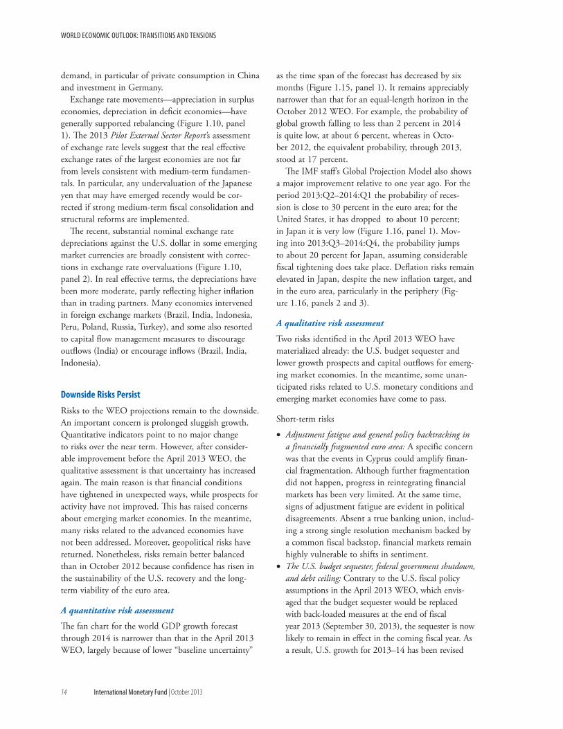
The fan chart for the world GDP growth forecast through 2014 is narrower than that in the April 2013 WEO, largely because of lower “baseline uncertainty”
as the time span of the forecast has decreased by six months (Figure 1.15, panel 1). It remains appreciably narrower than that for an equal-length horizon in the October 2012 WEO. For example, the probability of global growth falling to less than 2 percent in 2014 is quite low, at about 6 percent, whereas in Octo-ber 2012, the equivalent probability, through 2013, stood at 17 percent.
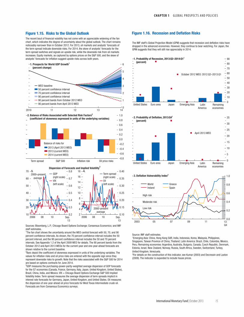
The IMF staff’s Global Projection Model also shows a major improvement relative to one year ago. For the period 2013:Q2–2014:Q1 the probability of reces-sion is close to 30 percent in the euro area; for the United States, it has dropped to about 10 percent; in Japan it is very low (Figure 1.16, panel 1). Mov-ing into 2013:Q3–2014:Q4, the probability jumps to about 20 percent for Japan, assuming considerable fiscal tightening does take place. Deflation risks remain elevated in Japan, despite the new inflation target, and in the euro area, particularly in the periphery (Fig-ure 1.16, panels 2 and 3).
A qualitative risk assessment
Two risks identified in the April 2013 WEO have materialized already: the U.S. budget sequester and lower growth prospects and capital outflows for emerg-ing market economies. In the meantime, some unan-ticipated risks related to U.S. monetary conditions and emerging market economies have come to pass.
Short-term risks
• Adjustment fatigue and general policy backtracking in a financially fragmented euro area: A specific concern was that the events in Cyprus could amplify finan-cial fragmentation. Although further fragmentation did not happen, progress in reintegrating financial markets has been very limited. At the same time, signs of adjustment fatigue are evident in political disagreements. Absent a true banking union, includ-ing a strong single resolution mechanism backed by a common fiscal backstop, financial markets remain highly vulnerable to shifts in sentiment.
• The U.S. budget sequester, federal government shutdown, and debt ceiling: Contrary to the U.S. fiscal policy assumptions in the April 2013 WEO, which envis-aged that the budget sequester would be replaced with back-loaded measures at the end of fiscal year 2013 (September 30, 2013), the sequester is now likely to remain in effect in the coming fiscal year. As a result, U.S. growth for 2013–14 has been revised
c h a p t e r 1 G lo b a l P r o s P e c ts a n d P o l i c i e s
international monetary Fund | October 2013 15
2
4
6
8
10
12
14
16
18
0.10
0.15
0.20
0.25
0.30
0.35
0.40
2006 08 10 Sep.13
0
1
2
3
4
5
6
2010 11 12 13 14
Figure 1.15. Risks to the Global Outlook
–0.8
–0.6
–0.4
–0.2
0.0
0.2
0.4
0.6
0.8
1.0
Term spread S&P 500 Inflation risk Oil price risks
10
20
30
40
50
60
70
0.2
0.3
0.4
0.5
0.6
0.7
0.8
2006 08 10 Sep.13
1. Prospects for World GDP Growth1
(percent change)
WEO baseline50 percent confidence interval70 percent confidence interval90 percent confidence interval90 percent bands from October 2012 WEO90 percent bands from April 2013 WEO
2. Balance of Risks Associated with Selected Risk Factors2
(coefficient of skewness expressed in units of the underlying variables)
2013 (April 2013 WEO)2013 (current WEO)2014 (current WEO)
Balance of risks for
Dispersion of Forecasts and Implied Volatility3
3. 4.2000–present
average
2000–presentaverage
GDP(right scale)VIX(left scale)
Term spread(right scale)Oil(left scale)
Sources: Bloomberg, L.P.; Chicago Board Options Exchange; Consensus Economics; and IMF staff estimates.1The fan chart shows the uncertainty around the WEO central forecast with 50, 70, and 90 percent confidence intervals. As shown, the 70 percent confidence interval includes the 50 percent interval, and the 90 percent confidence interval includes the 50 and 70 percent intervals. See Appendix 1.2 of the April 2009 WEO for details. The 90 percent bands from the October 2012 and April 2013 WEOs for the current-year and one-year-ahead forecasts are shown relative to the current baseline. 2Bars depict the coefficient of skewness expressed in units of the underlying variables. The values for inflation risks and oil price risks are entered with the opposite sign since they represent downside risks to growth. Note that the risks associated with the S&P 500 for 2014 are based on options contracts for June 2014. 3GDP measures the purchasing-power-parity-weighted average dispersion of GDP forecasts for the G7 economies (Canada, France, Germany, Italy, Japan, United Kingdom, United States), Brazil, China, India, and Mexico. VIX = Chicago Board Options Exchange S&P 500 Implied Volatility Index. Term spread measures the average dispersion of term spreads implicit in interest rate forecasts for Germany, Japan, United Kingdom, and United States. Oil measures the dispersion of one-year-ahead oil price forecasts for West Texas Intermediate crude oil. Forecasts are from Consensus Economics surveys.
The recent bout of financial volatility has not come with an appreciable widening of the fan chart, which indicates the degree of uncertainty about the global outlook. The chart remains noticeably narrower than in October 2012. For 2013, oil markets and analysts’ forecasts of the term spread indicate downside risks. For 2014, the skew of analysts’ forecasts for the term spread switches and signals an upside risk, while the downside risk from oil markets increases. Equity markets, as captured by options prices on the S&P 500, and the skew of analysts’ forecasts for inflation suggest upside risks across both years.
0
10
20
30
40
50
60
70
80
90
United States Euro area Japan Emerging Asia LatinAmerica
Remainingeconomies
Source: IMF staff estimates. 1Emerging Asia: China, Hong Kong SAR, India, Indonesia, Korea, Malaysia, Philippines, Singapore, Taiwan Province of China, Thailand; Latin America: Brazil, Chile, Colombia, Mexico, Peru; Remaining economies: Argentina, Australia, Bulgaria, Canada, Czech Republic, Denmark, Estonia, Israel, New Zealand, Norway, Russia, South Africa, Sweden, Switzerland, Turkey, United Kingdom, Venezuela.2For details on the construction of this indicator, see Kumar (2003) and Decressin and Laxton (2009). The indicator is expanded to include house prices.
Figure 1.16. Recession and Deflation Risks
The IMF staff’s Global Projection Model (GPM) suggests that recession and deflation risks have dropped in the advanced economies. However, they continue to bear watching. For Japan, the GPM suggests that they will still rise appreciably in 2014.
0
5
10
15
20
25
30
35
United States Euro area Japan Emerging Asia LatinAmerica
Remainingeconomies
0.0
0.2
0.4
0.6
0.8
1.0
2003 05 07 09 11 13:Q4
1. Probability of Recession, 2013:Q2–2014:Q11
(percent)
2. Probability of Deflation, 2013:Q41
(percent)
3. Deflation Vulnerability Index2
High risk
Moderate risk
Low risk
October 2012 WEO: 2012:Q2–2013:Q1
World GreeceIreland Spain
April 2013 WEO
world economic outlook: transitions and tensions
16 international monetary Fund | October 2013
downward in the July WEO Update, but the drag could be larger than expected given tighter financial conditions. The damage to the U.S. economy from a short government shutdown is likely to be limited, but a longer shutdown could be quite harmful. Even more importantly, the debt ceiling will need to be raised again later this year; failure to do so promptly could seriously damage the global economy.
• Risks related to unconventional monetary policy: The April 2013 WEO saw those risks mainly for the medium term (see below). But statements by the Federal Reserve about tapering asset purchases later this year caused a surprisingly large tightening of U.S. monetary conditions. A further surprise is the jump in emerging market local bond yields, which is roughly three times the level consistent with the U.S. monetary tightening scenario of the April 2013 WEO. The current WEO projections assume that the tightening of financial conditions since May in the United States and in many emerging market economies was largely a one-time event and that the actual taper-ing of purchases will further tighten conditions only modestly. However, a less benign scenario is a distinct risk to the extent that international capital flows were driven more by low yields in advanced economies than better growth prospects in emerging market economies.
• More disappointments in emerging markets: The risk of more disappointments could interact with the “unwinding” risks. Although net capital flows to emerging market economies are projected to remain sizable in the WEO forecast, policymakers must be mindful of risks of an abrupt cutoff and severe balance of payments disruptions. Fixed-income and emerg-ing market asset quality may have passed the peak, and the leveraged positions that were built up dur-ing the period of low policy rates and high emerging market growth might well be unwound more rapidly than expected. Adverse feedback loops could emerge between further growth disappointments, weakening balance sheets, and tighter external funding condi-tions—especially in economies that relied heavily on external funding to support credit-driven growth.
• Geopolitical risks: A short-lived, small disruption to oil production with an oil price spike of 10 to 20 percent for a few weeks would only have minor effects on global growth, if it is clear at the outset that it will be short-lived (see the Special Feature). If not, confidence and uncertainty effects would also weigh on activity. Larger, longer-lasting production outages and price spikes would have
bigger effects on growth, as other, amplifying trans-mission channels would come into play, including investor flight to safety and significant corrections in stock markets. Emerging market economies that are already seeing a pullback of investors and weak domestic fundamentals could be hit hard.
Medium-term risks
The medium-term risks discussed in detail in the April 2013 WEO are as relevant as they were then and tilt to the downside: (1) very low growth or stagnation in the euro area; (2) fiscal trouble in the United States or Japan––for Japan, the October 2013 GFSR specifically discusses a tail risk scenario of “disorderly Abenomics”; (3) less slack than expected in the advanced economies or a sudden burst of inflation; and (4) less potential output in key emerging market economies plus capital outflows.
A plausible downside scenario
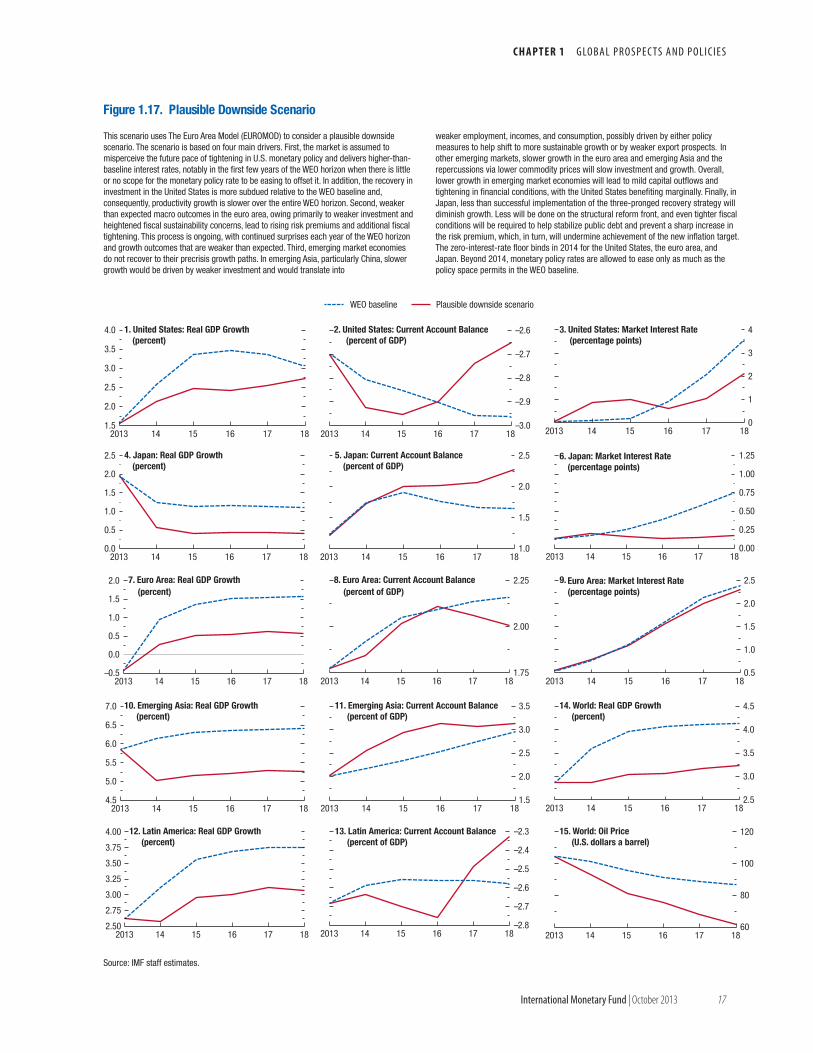
A likely scenario for the global economy is one of continued, plausible disappointments everywhere. These disappointments could include the following (Figure 1.17): • Investment and growth stay weak in the euro area,
as policies fail to resolve financial fragmentation and fail to inspire confidence among investors.
• Growth in emerging market and developing econo-mies softens further, and growth in China is lower in the medium term as the shift toward consump-tion-driven growth proves more complicated than expected. This has repercussions via trade and lower commodity prices.
• Policy implementation in Japan is incomplete. In particular, the scenario incorporates shortfalls in structural reforms, a failure of inflation expectations to durably move up to 2 percent, and consequently, more fiscal tightening to contain the debt-GDP ratio and prevent sharp increases in the risk pre-mium on Japanese government bonds.
• U.S. financial conditions tighten more than assumed in the WEO forecast over the coming year. Also, private investment does not recover as forecast, and, consequently potential growth turns out lower than expected. Tighter financial conditions than assumed in the WEO projections are already partly priced into markets, and the scenario assumes that mar-ket rates increase further when the Federal Reserve tapers its asset purchases. Such overtightened finan-cial conditions may be difficult to reverse in a timely manner because damage to the economy is observed
c h a p t e r 1 G lo b a l P r o s P e c ts a n d P o l i c i e s
international monetary Fund | October 2013 17
2.50
2.75
3.00
3.25
3.50
3.75
4.00
2013 14 15 16 17 18
–3.0
–2.9
–2.8
–2.7
–2.6
2013 14 15 16 17 180
1
2
3
4
2013 14 15 16 17 18
1.0
1.5
2.0
2.5
2013 14 15 16 17 18
1.75
2.00
2.25
2013 14 15 16 17 18
1.5
2.0
2.5
3.0
3.5
4.0
2013 14 15 16 17 18
Figure 1.17. Plausible Downside Scenario
1. United States: Real GDP Growth(percent)
2. United States: Current Account Balance(percent of GDP)
3. United States: Market Interest Rate(percentage points)
Source: IMF staff estimates.
0.0
0.5
1.0
1.5
2.0
2.5
2013 14 15 16 17 180.00
0.25
0.50
0.75
1.00
1.25
2013 14 15 16 17 18
–0.5
0.0
0.5
1.0
1.5
2.0
2013 14 15 16 17 180.5
1.0
1.5
2.0
2.5
2013 14 15 16 17 18
4. Japan: Real GDP Growth(percent)
5. Japan: Current Account Balance(percent of GDP)
6. Japan: Market Interest Rate(percentage points)
7. Euro Area: Real GDP Growth(percent)
8. Euro Area: Current Account Balance(percent of GDP)
9. Euro Area: Market Interest Rate(percentage points)
1.5
2.0
2.5
3.0
3.5
2013 14 15 16 17 184.5
5.0
5.5
6.0
6.5
7.0
2013 14 15 16 17 18
10. Emerging Asia: Real GDP Growth(percent)
11. Emerging Asia: Current Account Balance(percent of GDP)
12. Latin America: Real GDP Growth(percent)
2.5
3.0
3.5
4.0
4.5
2013 14 15 16 17 18
–2.8
–2.7
–2.6
–2.5
–2.4
–2.3
2013 14 15 16 17 1860
80
100
120
2013 14 15 16 17 18
13. Latin America: Current Account Balance(percent of GDP)
14. World: Real GDP Growth(percent)
15. World: Oil Price(U.S. dollars a barrel)
WEO baseline Plausible downside scenario
This scenario uses The Euro Area Model (EUROMOD) to consider a plausible downside scenario. The scenario is based on four main drivers. First, the market is assumed to misperceive the future pace of tightening in U.S. monetary policy and delivers higher-than-baseline interest rates, notably in the first few years of the WEO horizon when there is little or no scope for the monetary policy rate to be easing to offset it. In addition, the recovery in investment in the United States is more subdued relative to the WEO baseline and, consequently, productivity growth is slower over the entire WEO horizon. Second, weaker than expected macro outcomes in the euro area, owing primarily to weaker investment and heightened fiscal sustainability concerns, lead to rising risk premiums and additional fiscal tightening. This process is ongoing, with continued surprises each year of the WEO horizon and growth outcomes that are weaker than expected. Third, emerging market economies do not recover to their precrisis growth paths. In emerging Asia, particularly China, slower growth would be driven by weaker investment and would translate into
weaker employment, incomes, and consumption, possibly driven by either policy measures to help shift to more sustainable growth or by weaker export prospects. In other emerging markets, slower growth in the euro area and emerging Asia and the repercussions via lower commodity prices will slow investment and growth. Overall, lower growth in emerging market economies will lead to mild capital outflows and tightening in financial conditions, with the United States benefiting marginally. Finally, in Japan, less than successful implementation of the three-pronged recovery strategy will diminish growth. Less will be done on the structural reform front, and even tighter fiscal conditions will be required to help stabilize public debt and prevent a sharp increase in the risk premium, which, in turn, will undermine achievement of the new inflation target. The zero-interest-rate floor binds in 2014 for the United States, the euro area, and Japan. Beyond 2014, monetary policy rates are allowed to ease only as much as the policy space permits in the WEO baseline.
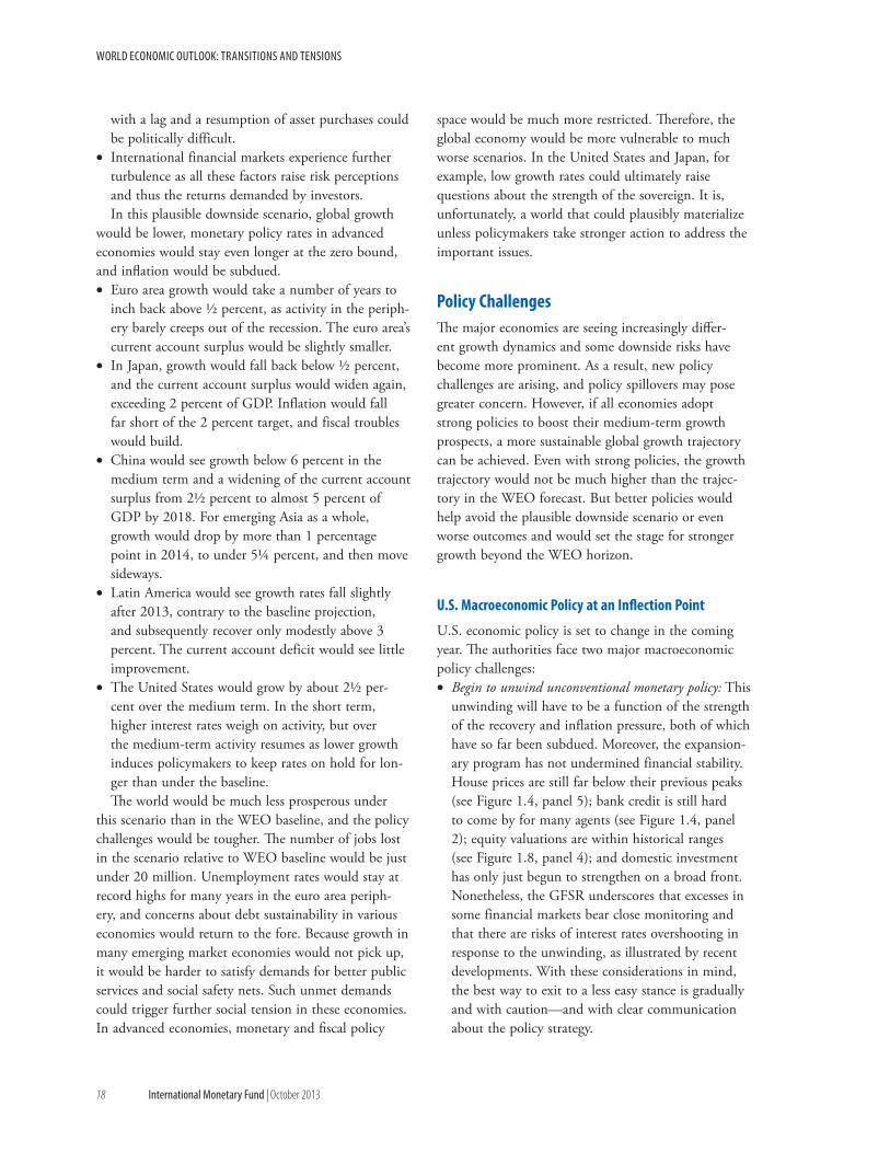
world economic outlook: transitions and tensions
18 international monetary Fund | October 2013
with a lag and a resumption of asset purchases could be politically difficult.
• International financial markets experience further turbulence as all these factors raise risk perceptions and thus the returns demanded by investors.In this plausible downside scenario, global growth
would be lower, monetary policy rates in advanced economies would stay even longer at the zero bound, and inflation would be subdued. • Euro area growth would take a number of years to
inch back above ½ percent, as activity in the periph-ery barely creeps out of the recession. The euro area’s current account surplus would be slightly smaller.
• In Japan, growth would fall back below ½ percent, and the current account surplus would widen again, exceeding 2 percent of GDP. Inflation would fall far short of the 2 percent target, and fiscal troubles would build.
• China would see growth below 6 percent in the medium term and a widening of the current account surplus from 2½ percent to almost 5 percent of GDP by 2018. For emerging Asia as a whole, growth would drop by more than 1 percentage point in 2014, to under 5¼ percent, and then move sideways.
• Latin America would see growth rates fall slightly after 2013, contrary to the baseline projection, and subsequently recover only modestly above 3 percent. The current account deficit would see little improvement.
• The United States would grow by about 2½ per-cent over the medium term. In the short term, higher interest rates weigh on activity, but over the medium-term activity resumes as lower growth induces policymakers to keep rates on hold for lon-ger than under the baseline.The world would be much less prosperous under
this scenario than in the WEO baseline, and the policy challenges would be tougher. The number of jobs lost in the scenario relative to WEO baseline would be just under 20 million. Unemployment rates would stay at record highs for many years in the euro area periph-ery, and concerns about debt sustainability in various economies would return to the fore. Because growth in many emerging market economies would not pick up, it would be harder to satisfy demands for better public services and social safety nets. Such unmet demands could trigger further social tension in these economies. In advanced economies, monetary and fiscal policy
space would be much more restricted. Therefore, the global economy would be more vulnerable to much worse scenarios. In the United States and Japan, for example, low growth rates could ultimately raise questions about the strength of the sovereign. It is, unfortunately, a world that could plausibly materialize unless policymakers take stronger action to address the important issues.
policy challengesThe major economies are seeing increasingly differ-ent growth dynamics and some downside risks have become more prominent. As a result, new policy challenges are arising, and policy spillovers may pose greater concern. However, if all economies adopt strong policies to boost their medium-term growth prospects, a more sustainable global growth trajectory can be achieved. Even with strong policies, the growth trajectory would not be much higher than the trajec-tory in the WEO forecast. But better policies would help avoid the plausible downside scenario or even worse outcomes and would set the stage for stronger growth beyond the WEO horizon.
U.S. Macroeconomic policy at an Inflection point
U.S. economic policy is set to change in the coming year. The authorities face two major macroeconomic policy challenges: • Begin to unwind unconventional monetary policy: This
unwinding will have to be a function of the strength of the recovery and inflation pressure, both of which have so far been subdued. Moreover, the expansion-ary program has not undermined financial stability. House prices are still far below their previous peaks (see Figure 1.4, panel 5); bank credit is still hard to come by for many agents (see Figure 1.4, panel 2); equity valuations are within historical ranges (see Figure 1.8, panel 4); and domestic investment has only just begun to strengthen on a broad front. Nonetheless, the GFSR underscores that excesses in some financial markets bear close monitoring and that there are risks of interest rates overshooting in response to the unwinding, as illustrated by recent developments. With these considerations in mind, the best way to exit to a less easy stance is gradually and with caution—and with clear communication about the policy strategy.
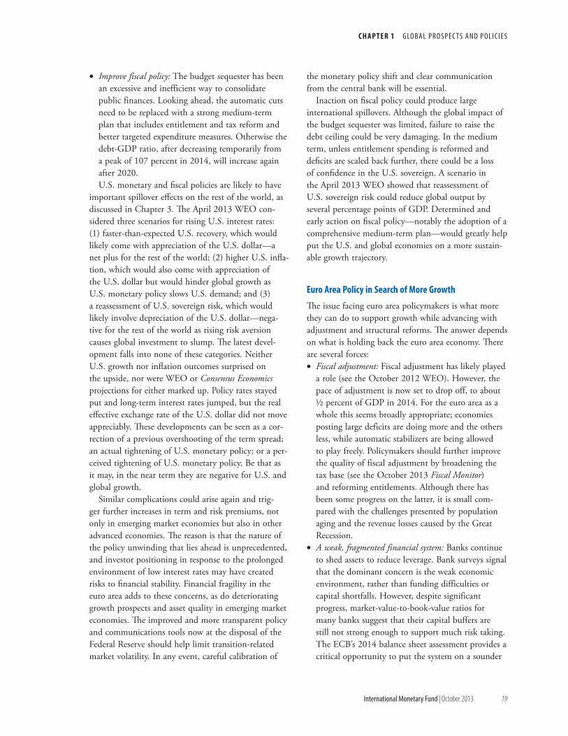
c h a p t e r 1 G lo b a l P r o s P e c ts a n d P o l i c i e s
international monetary Fund | October 2013 19
• Improve fiscal policy: The budget sequester has been an excessive and inefficient way to consolidate public finances. Looking ahead, the automatic cuts need to be replaced with a strong medium-term plan that includes entitlement and tax reform and better targeted expenditure measures. Otherwise the debt-GDP ratio, after decreasing temporarily from a peak of 107 percent in 2014, will increase again after 2020. U.S. monetary and fiscal policies are likely to have
important spillover effects on the rest of the world, as discussed in Chapter 3. The April 2013 WEO con-sidered three scenarios for rising U.S. interest rates: (1) faster-than-expected U.S. recovery, which would likely come with appreciation of the U.S. dollar—a net plus for the rest of the world; (2) higher U.S. infla-tion, which would also come with appreciation of the U.S. dollar but would hinder global growth as U.S. monetary policy slows U.S. demand; and (3) a reassessment of U.S. sovereign risk, which would likely involve depreciation of the U.S. dollar—nega-tive for the rest of the world as rising risk aversion causes global investment to slump. The latest devel-opment falls into none of these categories. Neither U.S. growth nor inflation outcomes surprised on the upside, nor were WEO or Consensus Economics projections for either marked up. Policy rates stayed put and long-term interest rates jumped, but the real effective exchange rate of the U.S. dollar did not move appreciably. These developments can be seen as a cor-rection of a previous overshooting of the term spread; an actual tightening of U.S. monetary policy; or a per-ceived tightening of U.S. monetary policy. Be that as it may, in the near term they are negative for U.S. and global growth.
Similar complications could arise again and trig-ger further increases in term and risk premiums, not only in emerging market economies but also in other advanced economies. The reason is that the nature of the policy unwinding that lies ahead is unprecedented, and investor positioning in response to the prolonged environment of low interest rates may have created risks to financial stability. Financial fragility in the euro area adds to these concerns, as do deteriorating growth prospects and asset quality in emerging market economies. The improved and more transparent policy and communications tools now at the disposal of the Federal Reserve should help limit transition-related market volatility. In any event, careful calibration of
the monetary policy shift and clear communication from the central bank will be essential.
Inaction on fiscal policy could produce large international spillovers. Although the global impact of the budget sequester was limited, failure to raise the debt ceiling could be very damaging. In the medium term, unless entitlement spending is reformed and deficits are scaled back further, there could be a loss of confidence in the U.S. sovereign. A scenario in the April 2013 WEO showed that reassessment of U.S. sovereign risk could reduce global output by several percentage points of GDP. Determined and early action on fiscal policy—notably the adoption of a comprehensive medium-term plan—would greatly help put the U.S. and global economies on a more sustain-able growth trajectory.
euro area policy in Search of More Growth
The issue facing euro area policymakers is what more they can do to support growth while advancing with adjustment and structural reforms. The answer depends on what is holding back the euro area economy. There are several forces: • Fiscal adjustment: Fiscal adjustment has likely played
a role (see the October 2012 WEO). However, the pace of adjustment is now set to drop off, to about ½ percent of GDP in 2014. For the euro area as a whole this seems broadly appropriate; economies posting large deficits are doing more and the others less, while automatic stabilizers are being allowed to play freely. Policymakers should further improve the quality of fiscal adjustment by broadening the tax base (see the October 2013 Fiscal Monitor) and reforming entitlements. Although there has been some progress on the latter, it is small com-pared with the challenges presented by population aging and the revenue losses caused by the Great Recession.
• A weak, fragmented financial system: Banks continue to shed assets to reduce leverage. Bank surveys signal that the dominant concern is the weak economic environment, rather than funding difficulties or capital shortfalls. However, despite significant progress, market-value-to-book-value ratios for many banks suggest that their capital buffers are still not strong enough to support much risk taking. The ECB’s 2014 balance sheet assessment provides a critical opportunity to put the system on a sounder
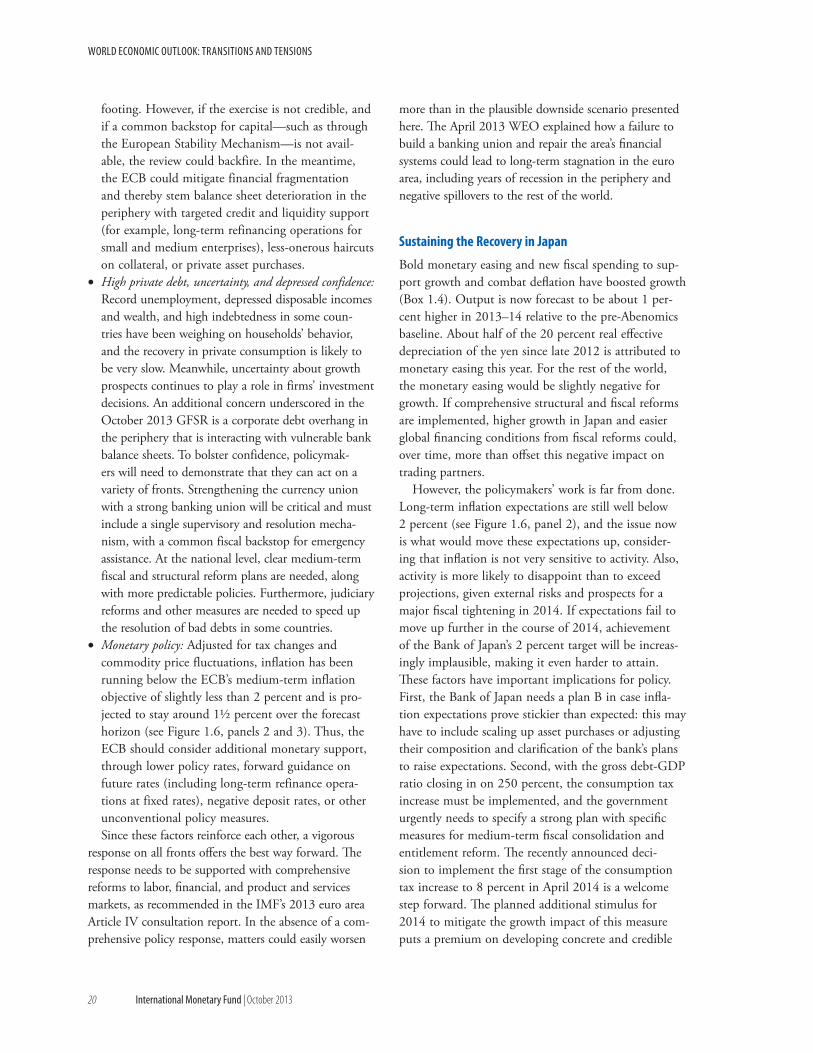
world economic outlook: transitions and tensions
20 international monetary Fund | October 2013
footing. However, if the exercise is not credible, and if a common backstop for capital—such as through the European Stability Mechanism—is not avail-able, the review could backfire. In the meantime, the ECB could mitigate financial fragmentation and thereby stem balance sheet deterioration in the periphery with targeted credit and liquidity support (for example, long-term refinancing operations for small and medium enterprises), less-onerous haircuts on collateral, or private asset purchases.
• High private debt, uncertainty, and depressed confidence: Record unemployment, depressed disposable incomes and wealth, and high indebtedness in some coun-tries have been weighing on households’ behavior, and the recovery in private consumption is likely to be very slow. Meanwhile, uncertainty about growth prospects continues to play a role in firms’ investment decisions. An additional concern underscored in the October 2013 GFSR is a corporate debt overhang in the periphery that is interacting with vulnerable bank balance sheets. To bolster confidence, policymak-ers will need to demonstrate that they can act on a variety of fronts. Strengthening the currency union with a strong banking union will be critical and must include a single supervisory and resolution mecha-nism, with a common fiscal backstop for emergency assistance. At the national level, clear medium-term fiscal and structural reform plans are needed, along with more predictable policies. Furthermore, judiciary reforms and other measures are needed to speed up the resolution of bad debts in some countries.
• Monetary policy: Adjusted for tax changes and commodity price fluctuations, inflation has been running below the ECB’s medium-term inflation objective of slightly less than 2 percent and is pro-jected to stay around 1½ percent over the forecast horizon (see Figure 1.6, panels 2 and 3). Thus, the ECB should consider additional monetary support, through lower policy rates, forward guidance on future rates (including long-term refinance opera-tions at fixed rates), negative deposit rates, or other unconventional policy measures. Since these factors reinforce each other, a vigorous
response on all fronts offers the best way forward. The response needs to be supported with comprehensive reforms to labor, financial, and product and services markets, as recommended in the IMF’s 2013 euro area Article IV consultation report. In the absence of a com-prehensive policy response, matters could easily worsen
more than in the plausible downside scenario presented here. The April 2013 WEO explained how a failure to build a banking union and repair the area’s financial systems could lead to long-term stagnation in the euro area, including years of recession in the periphery and negative spillovers to the rest of the world.
Sustaining the recovery in Japan
Bold monetary easing and new fiscal spending to sup-port growth and combat deflation have boosted growth (Box 1.4). Output is now forecast to be about 1 per-cent higher in 2013–14 relative to the pre-Abenomics baseline. About half of the 20 percent real effective depreciation of the yen since late 2012 is attributed to monetary easing this year. For the rest of the world, the monetary easing would be slightly negative for growth. If comprehensive structural and fiscal reforms are implemented, higher growth in Japan and easier global financing conditions from fiscal reforms could, over time, more than offset this negative impact on trading partners.
However, the policymakers’ work is far from done. Long-term inflation expectations are still well below 2 percent (see Figure 1.6, panel 2), and the issue now is what would move these expectations up, consider-ing that inflation is not very sensitive to activity. Also, activity is more likely to disappoint than to exceed projections, given external risks and prospects for a major fiscal tightening in 2014. If expectations fail to move up further in the course of 2014, achievement of the Bank of Japan’s 2 percent target will be increas-ingly implausible, making it even harder to attain. These factors have important implications for policy. First, the Bank of Japan needs a plan B in case infla-tion expectations prove stickier than expected: this may have to include scaling up asset purchases or adjusting their composition and clarification of the bank’s plans to raise expectations. Second, with the gross debt-GDP ratio closing in on 250 percent, the consumption tax increase must be implemented, and the government urgently needs to specify a strong plan with specific measures for medium-term fiscal consolidation and entitlement reform. The recently announced deci-sion to implement the first stage of the consumption tax increase to 8 percent in April 2014 is a welcome step forward. The planned additional stimulus for 2014 to mitigate the growth impact of this measure puts a premium on developing concrete and credible
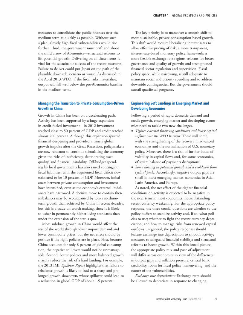
c h a p t e r 1 G lo b a l P r o s P e c ts a n d P o l i c i e s
international monetary Fund | October 2013 21
measures to consolidate the public finances over the medium term as quickly as possible. Without such a plan, already high fiscal vulnerabilities would rise further. Third, the government must craft and shoot the third arrow of Abenomics—structural reforms to lift potential growth. Delivering on all these fronts is vital for the sustainable success of the recent measures. Failure to deliver could put Japan on the path of the plausible downside scenario or worse. As discussed in the April 2013 WEO, if the fiscal risks materialize, output will fall well below the pre-Abenomics baseline in the medium term.
Managing the transition to private-consumption-Driven Growth in china
Growth in China has been on a decelerating path. Activity has been supported by a huge expansion in credit-fueled investment—in 2012 investment reached close to 50 percent of GDP and credit reached almost 200 percent. Although this expansion spurred financial deepening and provided a timely global growth impulse after the Great Recession, policymakers are now reluctant to continue stimulating the economy given the risks of inefficiency, deteriorating asset quality, and financial instability. Off-budget spend-ing by local governments has also raised contingent fiscal liabilities, with the augmented fiscal deficit now estimated to be 10 percent of GDP. Moreover, imbal-ances between private consumption and investment have intensified, even as the economy’s external imbal-ances have narrowed. A decisive move to contain these imbalances may be accompanied by lower medium-term growth than achieved by China in recent decades, but this is a trade-off worth making, since it is likely to usher in permanently higher living standards than under the extension of the status quo.
More subdued growth in China would affect the rest of the world through lower import demand and lower commodity prices, but the net effect should be positive if the right policies are in place. First, because China accounts for only 8 percent of global consump-tion, the negative spillovers would not be unmanage-able. Second, better policies and more balanced growth sharply reduce the risk of a hard landing. For example, the 2013 IMF Spillover Report highlights that failure to rebalance growth is likely to lead to a sharp and pro-longed growth slowdown, whose spillover could lead to a reduction in global GDP of about 1.5 percent.
The key priority is to maneuver a smooth shift to more sustainable, private-consumption-based growth. This shift would require liberalizing interest rates to allow effective pricing of risk; a more transparent, interest-rate-based monetary policy framework; a more flexible exchange rate regime; reforms for better governance and quality of growth; and strengthened financial sector regulation and supervision. Fiscal policy space, while narrowing, is still adequate to maintain social and priority spending and to address downside contingencies. But the government should curtail quasifiscal programs.
engineering Soft Landings in emerging Market and Developing economies
Following a period of rapid domestic demand and credit growth, emerging market and developing econo-mies need to tackle two new challenges. • Tighter external financing conditions and lower capital
inflows over the WEO horizon: These will come with the strengthening of the recovery in advanced economies and the normalization of U.S. monetary policy. Moreover, there is a risk of further bouts of volatility in capital flows and, for some economies, of severe balance of payments disruptions.
• Some slowing in potential growth and a cooldown from cyclical peaks: Accordingly, negative output gaps are small in most emerging market economies in Asia, Latin America, and Europe.As noted, the net effect of the tighter financial
conditions on activity is expected to be negative in the near term in most economies, notwithstanding recent currency weakening. For the appropriate policy response, the three crucial questions are whether to use policy buffers to stabilize activity and, if so, what poli-cies to use; whether to fight the recent currency depre-ciation; and how to manage risks from renewed capital outflows. In general, the policy responses should feature exchange rate depreciation to smooth activity; measures to safeguard financial stability; and structural reforms to boost growth. Within this broad picture, the appropriate policy mix and pace of adjustment will differ across economies in view of the differences in output gaps and inflation pressure, central bank credibility, room for fiscal policy maneuvering, and the nature of the vulnerabilities.
Exchange rate depreciation: Exchange rates should be allowed to depreciate in response to changing
world economic outlook: transitions and tensions
22 international monetary Fund | October 2013
fundamentals but policymakers need to guard against disorderly adjustment. Both structural and cyclical slowdowns in activity call for a depreciation of the real exchange rate, all else equal. Such a move would also help redress current account deficits in a few major emerging market economies whose deficits are larger than warranted by fundamentals and desired policies (Brazil, Indonesia, Turkey, South Africa).
Liquidity provision and exchange market interven-tion: This may be needed to maintain orderly condi-tions when very rapid flows lead to financial market disruption. Risks of disorderly conditions in currency markets are likely to be less acute for those economies that have strong policy frameworks, deeper financial markets, sound balance sheets, and limited non-resi-dent portfolio investment. While some intervention to smooth current market volatility may be appropriate in countries with adequate reserves, it should not forestall underlying external adjustment for those economies where external deficits exceed levels warranted by fundamentals and desired policies. In economies with pegged currencies, running down reserves is the natural response. However, even in those cases it should serve to ease but not postpone needed adjustments.
Monetary policy: Cyclical weakening of activity, in principle, calls for easing of monetary policies or, in economies where real interest rates are still low, less tightening than earlier planned. But, responses will need to consider inflationary pressures and policy credibility. In a number of economies, including Brazil, India, and Indonesia, more tightening may well be needed to address continued inflation pressure from capacity constraints, which will likely be reinforced by recent currency depreciation.
Prudential policies: Hefty exchange rate depreciation could lead to some increased solvency risk, especially for firms in the nontradables sectors, which do not enjoy a natural currency hedge in the form of export sales. Strong regulatory and supervisory policy efforts are needed to ensure that banks address credit quality and profitability problems, whether from legacy effects as a result of recent rapid credit growth in an envi-ronment with lower potential growth or from lower capital flows.
Fiscal policy: Policymakers should generally allow automatic stabilizers to respond freely but eschew stimulus, except when a major slowdown threatens. In many emerging market economies, growth is expected to remain fairly strong by historical standards. At the
same time, room for fiscal policy maneuvering has gen-erally declined. Fiscal deficits remain appreciably above precrisis levels (see Figure 1.5, panel 2). Moreover, while public debt ratios have mostly stabilized at rela-tively low levels, the debt dynamics are now projected to turn less favorable, given that real government bond yields are already some 100 basis points higher than expected at the time of the April WEO. Against this backdrop, there now is a broad need for policymakers to rebuild fiscal space in emerging market economies. As discussed in the October 2013 Fiscal Monitor, the urgency for action varies across economies: early, decisive steps are desirable in a few economies where public debt is already elevated (Brazil, Egypt, Hungary, India, Jordan, Poland, Malaysia). In some economies, increased contingent risks to budgets and public debt from substantial increases in quasifiscal activity and deficits reinforce the need to rebuild fiscal space (Bra-zil, China, Venezuela).
Structural reforms: Structural reforms to enhance productivity growth are a general priority, given the diagnostics of the growth slowdown. The lat-ter is in part a reflection of recent achievements in many emerging market economies. First, unlike the large advanced economies, many of these econo-mies have been operating near full capacity. Second, their incomes have been converging toward those in advanced economies, and as this income gap closes, growth in the emerging market economies is eventu-ally bound to decline. Even so, there is simultane-ously a need for even more catching up in incomes (“convergence”) and a risk that some of the capacity bottlenecks could create a middle-income trap, wherein relative wage increases end up reducing the com-petitiveness of these economies and thereby stalling growth. Many emerging market economies must focus on strengthening productivity in domestic services and other nontradables sectors, where there has been less progress than in tradables sectors, and on improving their investment regimes.
Many low-income economies have succeeded in maintaining strong growth during the weak global recovery. Structural policies fostering favorable business and investment regimes have been major contribu-tors to this outcome, as have better macroeconomic policies. With the decline in commodity prices and the increased costs of external financing, the external envi-ronment for these countries has become less favorable (see the Special Feature). Given these adverse changes,
c h a p t e r 1 G lo b a l P r o s P e c ts a n d P o l i c i e s
international monetary Fund | October 2013 23
timely adjustments to fiscal policies will be important; otherwise, external debt could build up again, as in past episodes.
rebalancing Global DemandWhat are the potential benefits from stronger policies? Policy simulations suggest that over the WEO horizon, the main benefit will be growth that is more balanced and sustained but not necessarily higher. An upside scenario examines the effects of stronger policies. The scenario is essentially the same scenario as in the 2013 Spillover Report, except that it also considers stron-ger policies in other emerging market economies, as follows: • In the near term, temporary measures in the United
Kingdom (fiscal and monetary) and the United States (fiscal) help support demand. In addition, the European authorities adopt measures to reduce financial fragmentation and implement a banking union. These actions reduce the cost of funding for the private and public sectors and stimulate investment.
• In the medium term, fiscal policy changes raise pub-lic saving in India, Japan, Russia, South Africa, and the United States. Tax reforms in India increase the incentives to work and invest. In addition, increased
public investment in infrastructure in South Africa stimulates private investment, increased efficiency in public spending in Russia allows for increased infrastructure investment, and pension reforms in Brazil and Russia support saving and invest-ment. Fiscal and financial reforms in China reduce both public and private saving and help rebalance demand toward private consumption and away from investment. Finally, structural reforms are under-taken in Brazil, the euro area, India, Japan, Russia, South Africa, and the United Kingdom that boost productivity and the labor supply. At the global level, these reforms have little impact
on growth because above-baseline growth in advanced economies and in Latin America in the near term is roughly offset by lower growth in emerging Asia, primarily China, because of the rebalancing. In the medium term, growth in China and emerging Asia returns to baseline, but the effects are offset by below-baseline growth in the United States and Japan owing to fiscal adjustment (Figure 1.18).
Although these policy measures have a negligible impact on global growth over the WEO horizon, they do reduce external imbalances. This, in turn, would make for a safer global economic environment, and help set the stage for more sustained and stronger growth in the long term.
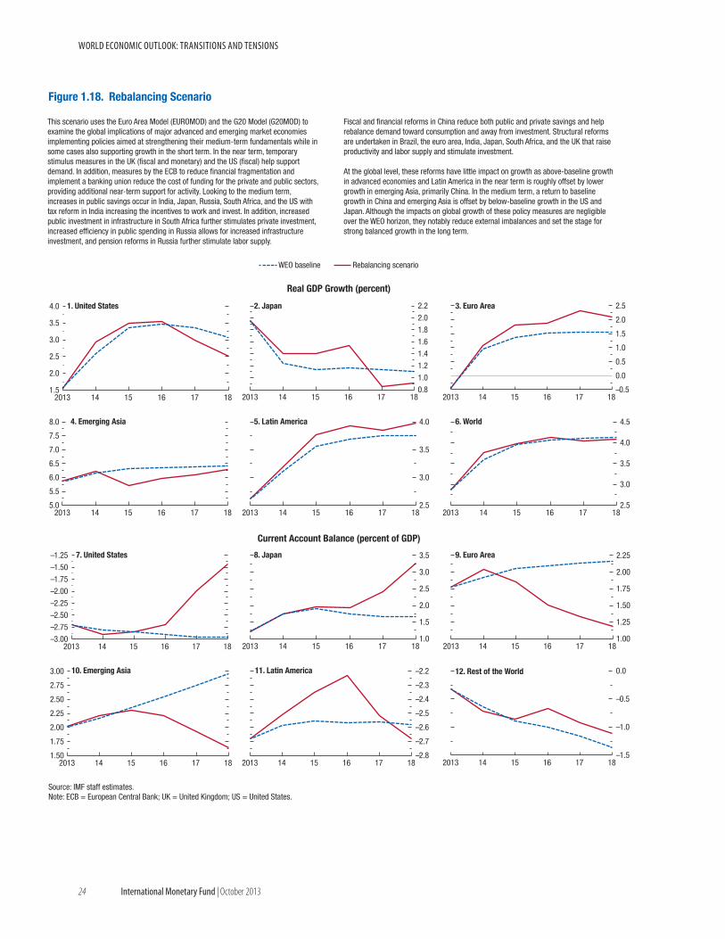
world economic outlook: transitions and tensions
24 international monetary Fund | October 2013
0.81.01.21.41.61.82.02.2
2013 14 15 16 17 18
Real GDP Growth (percent)
–0.5
0.0
0.5
1.0
1.5
2.0
2.5
2013 14 15 16 17 18
2.5
3.0
3.5
4.0
2013 14 15 16 17 18
1.0
1.5
2.0
2.5
3.0
3.5
2013 14 15 16 17 18
1.5
2.0
2.5
3.0
3.5
4.0
2013 14 15 16 17 18
Figure 1.18. Rebalancing Scenario
1. United States 2. Japan 3. Euro Area
Source: IMF staff estimates.Note: ECB = European Central Bank; UK = United Kingdom; US = United States.
5.0
5.5
6.0
6.5
7.0
7.5
8.0
2013 14 15 16 17 182.5
3.0
3.5
4.0
4.5
2013 14 15 16 17 18
–3.00–2.75–2.50–2.25–2.00–1.75–1.50–1.25
2013 14 15 16 17 181.00
1.25
1.50
1.75
2.00
2.25
2013 14 15 16 17 18
4. Emerging Asia 5. Latin America 6. World
–2.8
–2.7
–2.6
–2.5
–2.4
–2.3
–2.2
2013 14 15 16 17 181.50
1.75
2.00
2.25
2.50
2.75
3.00
2013 14 15 16 17 18–1.5
–1.0
–0.5
0.0
2013 14 15 16 17 18
Current Account Balance (percent of GDP)
WEO baseline Rebalancing scenario
7. United States 8. Japan 9. Euro Area
10. Emerging Asia 11. Latin America 12. Rest of the World
This scenario uses the Euro Area Model (EUROMOD) and the G20 Model (G20MOD) to examine the global implications of major advanced and emerging market economies implementing policies aimed at strengthening their medium-term fundamentals while in some cases also supporting growth in the short term. In the near term, temporary stimulus measures in the UK (fiscal and monetary) and the US (fiscal) help support demand. In addition, measures by the ECB to reduce financial fragmentation and implement a banking union reduce the cost of funding for the private and public sectors, providing additional near-term support for activity. Looking to the medium term, increases in public savings occur in India, Japan, Russia, South Africa, and the US with tax reform in India increasing the incentives to work and invest. In addition, increased public investment in infrastructure in South Africa further stimulates private investment, increased efficiency in public spending in Russia allows for increased infrastructure investment, and pension reforms in Russia further stimulate labor supply.
Fiscal and financial reforms in China reduce both public and private savings and help rebalance demand toward consumption and away from investment. Structural reforms are undertaken in Brazil, the euro area, India, Japan, South Africa, and the UK that raise productivity and labor supply and stimulate investment.
At the global level, these reforms have little impact on growth as above-baseline growth in advanced economies and Latin America in the near term is roughly offset by lower growth in emerging Asia, primarily China. In the medium term, a return to baseline growth in China and emerging Asia is offset by below-baseline growth in the US and Japan. Although the impacts on global growth of these policy measures are negligible over the WEO horizon, they notably reduce external imbalances and set the stage for strong balanced growth in the long term.
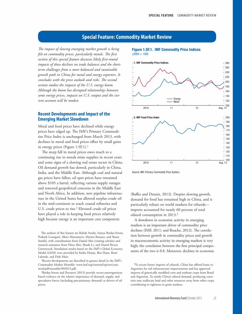
S p e c I a L F e at U r e co m m o d i t y ma r k e t r e v i e w
international monetary Fund | October 2013 25
The impact of slowing emerging market growth is being felt on commodity prices, particularly metals. The first section of this special feature discusses likely first-round impacts of these declines on trade balances and the short-term challenges from a more balanced and sustainable growth path in China for metal and energy exporters. It concludes with the price outlook and risks. The second section studies the impacts of the U.S. energy boom. Although the boom has disrupted relationships between some energy prices, impacts on U.S. output and the cur-rent account will be modest.
recent Developments and Impact of the emerging Market SlowdownMetal and food prices have declined while energy prices have edged up. The IMF’s Primary Commodi-ties Price Index is unchanged from March 2013, with declines in metal and food prices offset by small gains in energy prices (Figure 1.SF.1).1
The steep fall in metal prices owes much to a continuing rise in metals mine supplies in recent years and some signs of a slowing real estate sector in China. Oil demand growth has slowed, particularly in China, India, and the Middle East. Although coal and natural gas prices have fallen, oil spot prices have remained above $105 a barrel, reflecting various supply outages and renewed geopolitical concerns in the Middle East and North Africa. In addition, new pipeline infrastruc-ture in the United States has allowed surplus crude oil in the mid-continent to reach coastal refineries and U.S. crude prices to rise.2 Elevated crude oil prices have played a role in keeping food prices relatively high because energy is an important cost component
The authors of this feature are Rabah Arezki, Samya Beidas-Strom, Prakash Loungani, Akito Matsumoto, Marina Rousset, and Shane Streifel, with contributions from Daniel Ahn (visiting scholar) and research assistance from Hites Ahir, Shuda Li, and Daniel Rivera Greenwood. Simulation results based on the IMF’s Global Economy Model (GEM) were provided by Keiko Honjo, Ben Hunt, René Lalonde, and Dirk Muir.
1Recent developments are described in greater detail in the IMF’s Commodity Market Monthly: www.imf.org/external/np/res/com-mod/pdf/monthly/092013.pdf.
2Beidas-Strom and Pescatori (2013) provide vector-autoregression-based evidence on the relative importance of demand, supply, and speculative forces (including precautionary demand) as drivers of oil prices.
(Baffes and Dennis, 2013). Despite slowing growth, demand for food has remained high in China, and is particularly reliant on world markets for oilseeds—imports accounted for nearly 60 percent of total oilseed consumption in 2013.3
A slowdown in economic activity in emerging markets is an important driver of commodity price declines (IMF, 2011; and Roache, 2012). The correla-tion between growth in commodity prices and growth in macroeconomic activity in emerging markets is very high; the correlation between the first principal compo-nents of the two is 0.8. Moreover, declines in economic
3To secure future imports of oilseeds, China has offered loans to Argentina for rail infrastructure improvements and has approved imports of genetically modified corn and soybean crops from Brazil and Argentina. To satisfy China’s oilseed demand, producing coun-tries may reallocate land and other resources away from other crops, contributing to tightness in grain markets.
Special Feature: commodity Market review
100
120
140
160
180
200
220
240
260
280
2010 11 12 Aug. 13
Source: IMF, Primary Commodity Price System.
Figure 1.SF.1. IMF Commodity Price Indices(2005 = 100)
EnergyMetal
100
110
120
130
140
150
160
170
180
190
200
2010 11 12 Aug. 13
1. IMF Commodity Price Indices
2. IMF Food Price Index
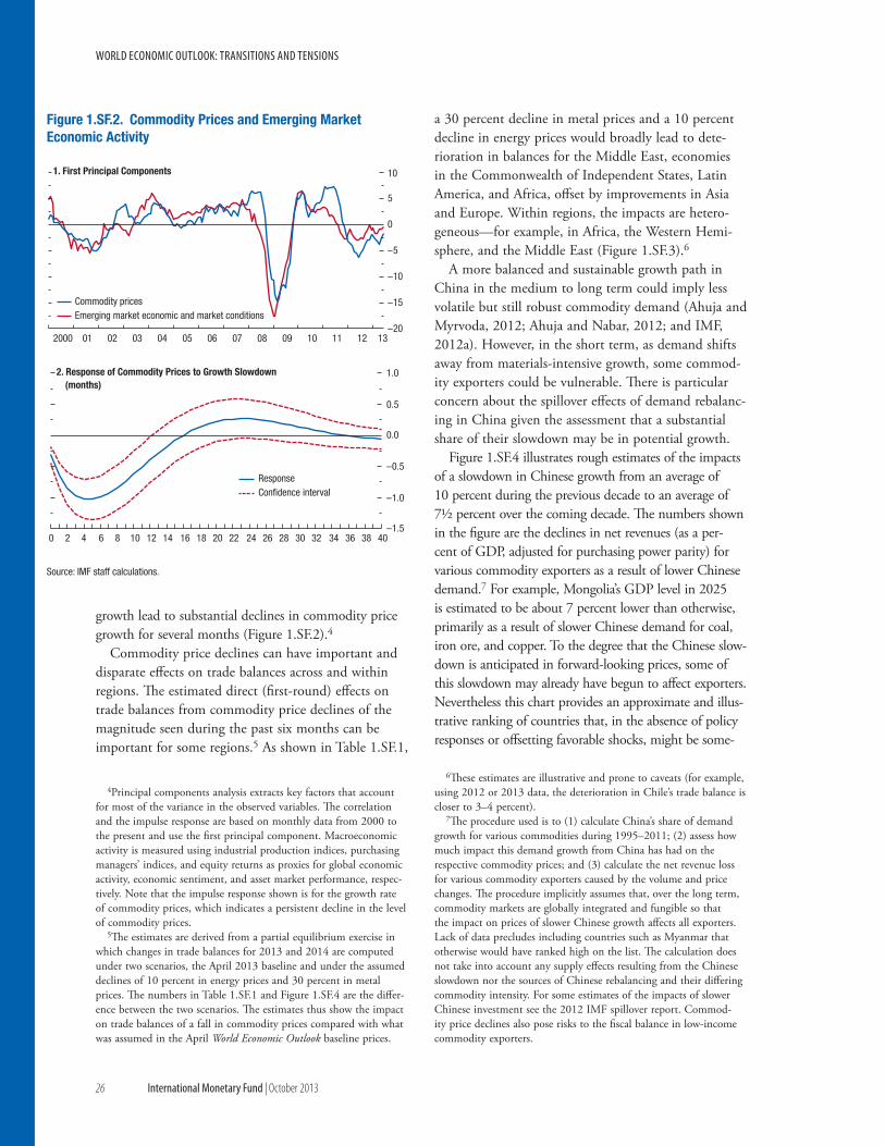
world economic outlook: transitions and tensions
26 international monetary Fund | October 2013
growth lead to substantial declines in commodity price growth for several months (Figure 1.SF.2).4
Commodity price declines can have important and disparate effects on trade balances across and within regions. The estimated direct (first-round) effects on trade balances from commodity price declines of the magnitude seen during the past six months can be important for some regions.5 As shown in Table 1.SF.1,
4Principal components analysis extracts key factors that account for most of the variance in the observed variables. The correlation and the impulse response are based on monthly data from 2000 to the present and use the first principal component. Macroeconomic activity is measured using industrial production indices, purchasing managers’ indices, and equity returns as proxies for global economic activity, economic sentiment, and asset market performance, respec-tively. Note that the impulse response shown is for the growth rate of commodity prices, which indicates a persistent decline in the level of commodity prices.
5The estimates are derived from a partial equilibrium exercise in which changes in trade balances for 2013 and 2014 are computed under two scenarios, the April 2013 baseline and under the assumed declines of 10 percent in energy prices and 30 percent in metal prices. The numbers in Table 1.SF.1 and Figure 1.SF.4 are the differ-ence between the two scenarios. The estimates thus show the impact on trade balances of a fall in commodity prices compared with what was assumed in the April World Economic Outlook baseline prices.
a 30 percent decline in metal prices and a 10 percent decline in energy prices would broadly lead to dete-rioration in balances for the Middle East, economies in the Commonwealth of Independent States, Latin America, and Africa, offset by improvements in Asia and Europe. Within regions, the impacts are hetero-geneous—for example, in Africa, the Western Hemi-sphere, and the Middle East (Figure 1.SF.3).6
A more balanced and sustainable growth path in China in the medium to long term could imply less volatile but still robust commodity demand (Ahuja and Myrvoda, 2012; Ahuja and Nabar, 2012; and IMF, 2012a). However, in the short term, as demand shifts away from materials-intensive growth, some commod-ity exporters could be vulnerable. There is particular concern about the spillover effects of demand rebalanc-ing in China given the assessment that a substantial share of their slowdown may be in potential growth.
Figure 1.SF.4 illustrates rough estimates of the impacts of a slowdown in Chinese growth from an average of 10 percent during the previous decade to an average of 7½ percent over the coming decade. The numbers shown in the figure are the declines in net revenues (as a per-cent of GDP, adjusted for purchasing power parity) for various commodity exporters as a result of lower Chinese demand.7 For example, Mongolia’s GDP level in 2025 is estimated to be about 7 percent lower than otherwise, primarily as a result of slower Chinese demand for coal, iron ore, and copper. To the degree that the Chinese slow-down is anticipated in forward-looking prices, some of this slowdown may already have begun to affect exporters. Nevertheless this chart provides an approximate and illus-trative ranking of countries that, in the absence of policy responses or offsetting favorable shocks, might be some-
6These estimates are illustrative and prone to caveats (for example, using 2012 or 2013 data, the deterioration in Chile’s trade balance is closer to 3–4 percent).
7The procedure used is to (1) calculate China’s share of demand growth for various commodities during 1995–2011; (2) assess how much impact this demand growth from China has had on the respective commodity prices; and (3) calculate the net revenue loss for various commodity exporters caused by the volume and price changes. The procedure implicitly assumes that, over the long term, commodity markets are globally integrated and fungible so that the impact on prices of slower Chinese growth affects all exporters. Lack of data precludes including countries such as Myanmar that otherwise would have ranked high on the list. The calculation does not take into account any supply effects resulting from the Chinese slowdown nor the sources of Chinese rebalancing and their differing commodity intensity. For some estimates of the impacts of slower Chinese investment see the 2012 IMF spillover report. Commod-ity price declines also pose risks to the fiscal balance in low-income commodity exporters.
–20
–15
–10
–5
0
5
10
2000 01 02 03 04 05 06 07 08 09 10 11 12 13
Source: IMF staff calculations.
Figure 1.SF.2. Commodity Prices and Emerging MarketEconomic Activity
Commodity pricesEmerging market economic and market conditions
–1.5
–1.0
–0.5
0.0
0.5
1.0
0 2 4 6 8 10 12 14 16 18 20 22 24 26 28 30 32 34 36 38 40
1. First Principal Components
2. Response of Commodity Prices to Growth Slowdown(months)
ResponseConfidence interval
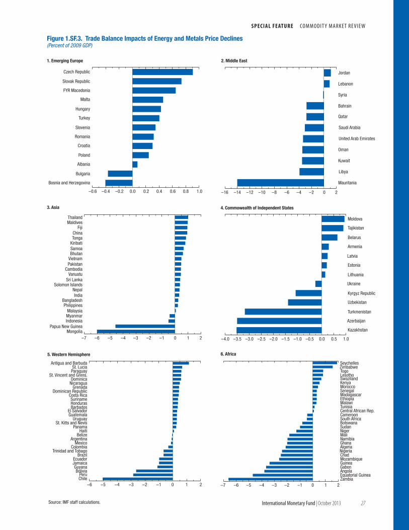
S p e c I a L F e at U r e co m m o d i t y ma r k e t r e v i e w
international monetary Fund | October 2013 27
–0.6 –0.4 –0.2 0.0 0.2 0.4 0.6 0.8 1.0
Bosnia and Herzegovina
Bulgaria
Albania
Poland
Croatia
Romania
Slovenia
Turkey
Hungary
Malta
FYR Macedonia
Slovak Republic
Czech Republic
–7 –6 –5 –4 –3 –2 –1 0 1 2Mongolia
Papua New GuineaIndonesiaMyanmarMalaysia
PhilippinesBangladesh
IndiaNepal
Solomon IslandsSri Lanka
VanuatuCambodia
PakistanVietnamBhutanSamoaKiribatiTongaChina
FijiMaldivesThailand
–6 –5 –4 –3 –2 –1 0 1 2ChilePeru
BoliviaGuyana
JamaicaEcuador
BrazilTrinidad and Tobago
ColombiaMexico
ArgentinaBelize
HaitiPanama
St. Kitts and NevisUruguay
GuatemalaEl Salvador
BarbadosHondurasSuriname
Costa RicaDominican Republic
GrenadaNicaraguaDominica
St. Vincent and Grens.ParaguaySt. Lucia
Antigua and Barbuda
Figure 1.SF.3. Trade Balance Impacts of Energy and Metals Price Declines(Percent of 2009 GDP)
1. Emerging Europe
Source: IMF staff calculations.
2. Middle East
–16 –14 –12 –10 –8 –6 –4 –2 0 2
Mauritania
Libya
Kuwait
Oman
United Arab Emirates
Saudi Arabia
Qatar
Bahrain
Syria
Lebanon
Jordan
3. Asia 4. Commowealth of Independent States
–4.0 –3.5 –3.0 –2.5 –2.0 –1.5 –1.0 –0.5 0.0 0.5 1.0
Kazakhstan
Azerbaijan
Turkmenistan
Uzbekistan
Kyrgyz Republic
Ukraine
Lithuania
Estonia
Latvia
Armenia
Belarus
Tajikistan
Moldova
5. Western Hemisphere 6. Africa
–7 –6 –5 –4 –3 –2 –1 0 1 2ZambiaEquatorial GuineaAngolaGabonGuineaMozambiqueChadNigeriaAlgeriaGhanaNamibiaMaliNigerSudanBotswanaSouth AfricaCameroonCentral African Rep.TunisiaMalawiEthiopiaMadagascarSenegalMoroccoKenyaSwazilandLesothoTogoZimbabweSeychelles
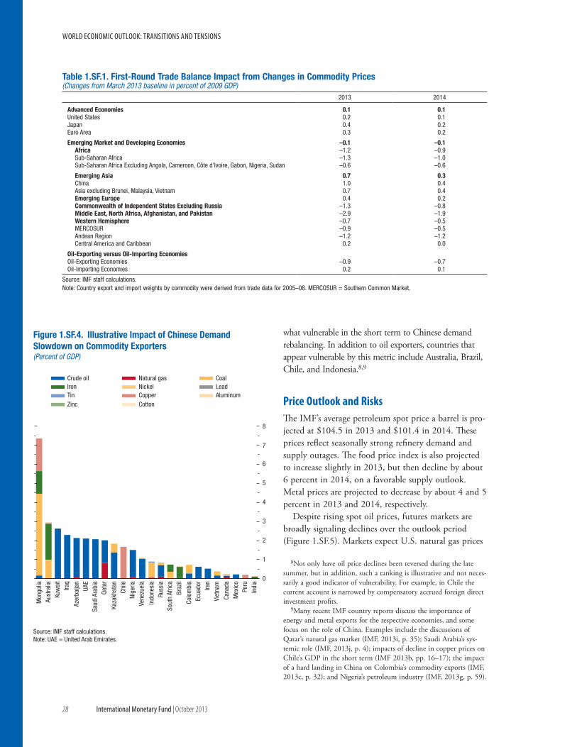
world economic outlook: transitions and tensions
28 international monetary Fund | October 2013
what vulnerable in the short term to Chinese demand rebalancing. In addition to oil exporters, countries that appear vulnerable by this metric include Australia, Brazil, Chile, and Indonesia.8,9
price Outlook and risksThe IMF’s average petroleum spot price a barrel is pro-jected at $104.5 in 2013 and $101.4 in 2014. These prices reflect seasonally strong refinery demand and supply outages. The food price index is also projected to increase slightly in 2013, but then decline by about 6 percent in 2014, on a favorable supply outlook. Metal prices are projected to decrease by about 4 and 5 percent in 2013 and 2014, respectively.
Despite rising spot oil prices, futures markets are broadly signaling declines over the outlook period (Figure 1.SF.5). Markets expect U.S. natural gas prices
8Not only have oil price declines been reversed during the late summer, but in addition, such a ranking is illustrative and not neces-sarily a good indicator of vulnerability. For example, in Chile the current account is narrowed by compensatory accrued foreign direct investment profits.
9Many recent IMF country reports discuss the importance of energy and metal exports for the respective economies, and some focus on the role of China. Examples include the discussions of Qatar’s natural gas market (IMF, 2013i, p. 35); Saudi Arabia’s sys-temic role (IMF, 2013j, p. 4); impacts of decline in copper prices on Chile’s GDP in the short term (IMF 2013b, pp. 16–17); the impact of a hard landing in China on Colombia’s commodity exports (IMF, 2013c, p. 32); and Nigeria’s petroleum industry (IMF, 2013g, p. 59).
0
1
2
3
4
5
6
7
8
Mon
golia
Aust
ralia
Kuw
ait
Iraq
Azer
baija
nUA
ESa
udi A
rabi
aQa
tar
Kaza
khst
anCh
ileNi
geria
Vene
zuel
a
Indo
nesi
aRu
ssia
Sout
h Af
rica
Braz
il
Colo
mbi
aEc
uado
r
Source: IMF staff calculations. Note: UAE = United Arab Emirates.
Figure 1.SF.4. Illustrative Impact of Chinese DemandSlowdown on Commodity Exporters(Percent of GDP)
Crude oil Natural gas CoalIron Nickel LeadTin Copper AluminumZinc Cotton
Viet
nam
Iran
Mex
ico
Cana
da
Indi
aPe
ru
Table 1.SF.1. First-Round Trade Balance Impact from Changes in Commodity Prices(Changes from March 2013 baseline in percent of 2009 GDP)
2013 2014
Advanced Economies 0.1 0.1United States 0.2 0.1Japan 0.4 0.2Euro Area 0.3 0.2
Emerging Market and Developing Economies –0.1 –0.1Africa –1.2 –0.9Sub-Saharan Africa –1.3 –1.0Sub-Saharan Africa Excluding Angola, Cameroon, Côte d’Ivoire, Gabon, Nigeria, Sudan –0.6 –0.6
Emerging Asia 0.7 0.3China 1.0 0.4Asia excluding Brunei, Malaysia, Vietnam 0.7 0.4Emerging Europe 0.4 0.2Commonwealth of Independent States Excluding Russia –1.3 –0.8Middle East, North Africa, Afghanistan, and Pakistan –2.9 –1.9Western Hemisphere –0.7 –0.5MERCOSUR –0.9 –0.5Andean Region –1.2 –1.2Central America and Caribbean 0.2 0.0
Oil-Exporting versus Oil-Importing EconomiesOil-Exporting Economies –0.9 –0.7Oil-Importing Economies 0.2 0.1
Source: IMF staff calculations.Note: Country export and import weights by commodity were derived from trade data for 2005–08. MERCOSUR = Southern Common Market.
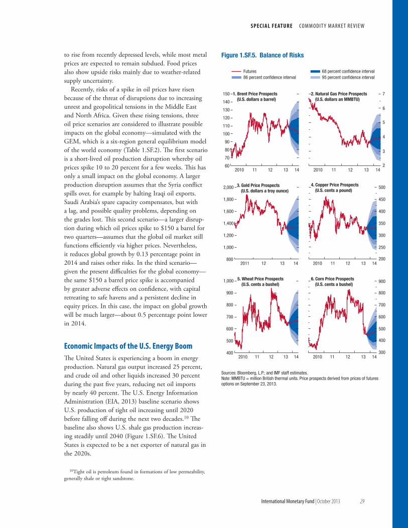
S p e c I a L F e at U r e co m m o d i t y ma r k e t r e v i e w
international monetary Fund | October 2013 29
to rise from recently depressed levels, while most metal prices are expected to remain subdued. Food prices also show upside risks mainly due to weather-related supply uncertainty.
Recently, risks of a spike in oil prices have risen because of the threat of disruptions due to increasing unrest and geopolitical tensions in the Middle East and North Africa. Given these rising tensions, three oil price scenarios are considered to illustrate possible impacts on the global economy—simulated with the GEM, which is a six-region general equilibrium model of the world economy (Table 1.SF.2). The first scenario is a short-lived oil production disruption whereby oil prices spike 10 to 20 percent for a few weeks. This has only a small impact on the global economy. A larger production disruption assumes that the Syria conflict spills over, for example by halting Iraqi oil exports. Saudi Arabia’s spare capacity compensates, but with a lag, and possible quality problems, depending on the grades lost. This second scenario—a larger disrup-tion during which oil prices spike to $150 a barrel for two quarters—assumes that the global oil market still functions efficiently via higher prices. Nevertheless, it reduces global growth by 0.13 percentage point in 2014 and raises other risks. In the third scenario—given the present difficulties for the global economy—the same $150 a barrel price spike is accompanied by greater adverse effects on confidence, with capital retreating to safe havens and a persistent decline in equity prices. In this case, the impact on global growth will be much larger—about 0.5 percentage point lower in 2014.
economic Impacts of the U.S. energy BoomThe United States is experiencing a boom in energy production. Natural gas output increased 25 percent, and crude oil and other liquids increased 30 percent during the past five years, reducing net oil imports by nearly 40 percent. The U.S. Energy Information Administration (EIA, 2013) baseline scenario shows U.S. production of tight oil increasing until 2020 before falling off during the next two decades.10 The baseline also shows U.S. shale gas production increas-ing steadily until 2040 (Figure 1.SF.6). The United States is expected to be a net exporter of natural gas in the 2020s.
10Tight oil is petroleum found in formations of low permeability, generally shale or tight sandstone.
200
250
300
350
400
450
500
2010 11 12 13 14
2
3
4
5
6
7
2010 11 12 13 14
Figure 1.SF.5. Balance of Risks
1. Brent Price Prospects(U.S. dollars a barrel)
Sources: Bloomberg, L.P.; and IMF staff estimates.Note: MMBTU = million British thermal units. Price prospects derived from prices of futures options on September 23, 2013.
Futures 68 percent confidence interval86 percent confidence interval 95 percent confidence interval
4. Copper Price Prospects(U.S. cents a pound)
3. Gold Price Prospects(U.S. dollars a troy ounce)
2. Natural Gas Price Prospects(U.S. dollars an MMBTU)
60
70
80
90
100
110
120
130
140
150
2010 11 12 13 14
5. Wheat Price Prospects(U.S. cents a bushel)
6. Corn Price Prospects(U.S. cents a bushel)
800
1,000
1,200
1,400
1,600
1,800
2,000
2011 12 13 14
400
500
600
700
800
900
1,000
2010 11 12 13 14300
400
500
600
700
800
900
2010 11 12 13 14
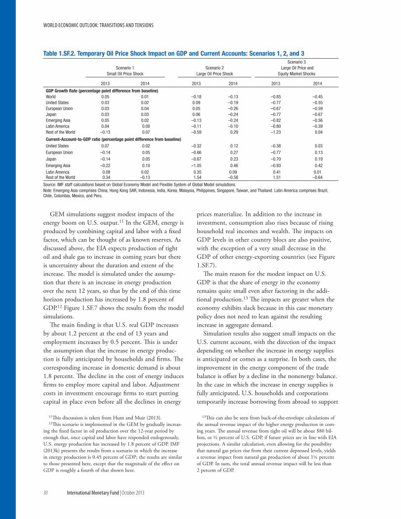
world economic outlook: transitions and tensions
30 international monetary Fund | October 2013
GEM simulations suggest modest impacts of the energy boom on U.S. output.11 In the GEM, energy is produced by combining capital and labor with a fixed factor, which can be thought of as known reserves. As discussed above, the EIA expects production of tight oil and shale gas to increase in coming years but there is uncertainty about the duration and extent of the increase. The model is simulated under the assump-tion that there is an increase in energy production over the next 12 years, so that by the end of this time horizon production has increased by 1.8 percent of GDP.12 Figure 1.SF.7 shows the results from the model simulations.
The main finding is that U.S. real GDP increases by about 1.2 percent at the end of 13 years and employment increases by 0.5 percent. This is under the assumption that the increase in energy produc-tion is fully anticipated by households and firms. The corresponding increase in domestic demand is about 1.8 percent. The decline in the cost of energy induces firms to employ more capital and labor. Adjustment costs in investment encourage firms to start putting capital in place even before all the declines in energy
11This discussion is taken from Hunt and Muir (2013).12This scenario is implemented in the GEM by gradually increas-
ing the fixed factor in oil production over the 12-year period by enough that, once capital and labor have responded endogenously, U.S. energy production has increased by 1.8 percent of GDP. IMF (2013k) presents the results from a scenario in which the increase in energy production is 0.45 percent of GDP; the results are similar to those presented here, except that the magnitude of the effect on GDP is roughly a fourth of that shown here.
prices materialize. In addition to the increase in investment, consumption also rises because of rising household real incomes and wealth. The impacts on GDP levels in other country blocs are also positive, with the exception of a very small decrease in the GDP of other energy-exporting countries (see Figure 1.SF.7).
The main reason for the modest impact on U.S. GDP is that the share of energy in the economy remains quite small even after factoring in the addi-tional production.13 The impacts are greater when the economy exhibits slack because in this case monetary policy does not need to lean against the resulting increase in aggregate demand.
Simulation results also suggest small impacts on the U.S. current account, with the direction of the impact depending on whether the increase in energy supplies is anticipated or comes as a surprise. In both cases, the improvement in the energy component of the trade balance is offset by a decline in the nonenergy balance. In the case in which the increase in energy supplies is fully anticipated, U.S. households and corporations temporarily increase borrowing from abroad to support
13This can also be seen from back-of-the-envelope calculations of the annual revenue impact of the higher energy production in com-ing years. The annual revenue from tight oil will be about $80 bil-lion, or ½ percent of U.S. GDP, if future prices are in line with EIA projections. A similar calculation, even allowing for the possibility that natural gas prices rise from their current depressed levels, yields a revenue impact from natural gas production of about 1¼ percent of GDP. In sum, the total annual revenue impact will be less than 2 percent of GDP.
Table 1.SF.2. Temporary Oil Price Shock Impact on GDP and Current Accounts: Scenarios 1, 2, and 3
Scenario 1Small Oil Price Shock
Scenario 2Large Oil Price Shock
Scenario 3 Large Oil Price and
Equity Market Shocks
2013 2014 2013 2014 2013 2014
GDP Growth Rate (percentage point difference from baseline)World 0.05 0.01 –0.18 –0.13 –0.85 –0.45United States 0.03 0.02 0.09 –0.19 –0.77 –0.55European Union 0.03 0.04 0.05 –0.26 –0.67 –0.59Japan 0.03 0.03 0.06 –0.24 –0.77 –0.67Emerging Asia 0.05 0.02 –0.13 –0.24 –0.82 –0.56Latin America 0.04 0.00 –0.11 –0.10 –0.80 –0.39Rest of the World –0.13 0.07 –0.59 0.29 –1.23 0.04
Current-Account-to-GDP ratio (percentage point difference from baseline)United States 0.07 0.02 –0.32 0.12 –0.38 0.03European Union –0.14 0.05 –0.66 0.27 –0.77 0.13Japan –0.14 0.05 –0.67 0.23 –0.70 0.19Emerging Asia –0.22 0.10 –1.05 0.46 –0.93 0.42Latin America 0.08 0.02 0.35 0.09 0.41 0.01Rest of the World 0.34 –0.13 1.54 –0.58 1.51 –0.64
Source: IMF staff calculations based on Global Economy Model and Flexible System of Global Model simulations.Note: Emerging Asia comprises China, Hong Kong SAR, Indonesia, India, Korea, Malaysia, Philippines, Singapore, Taiwan, and Thailand. Latin America comprises Brazil, Chile, Colombia, Mexico, and Peru.
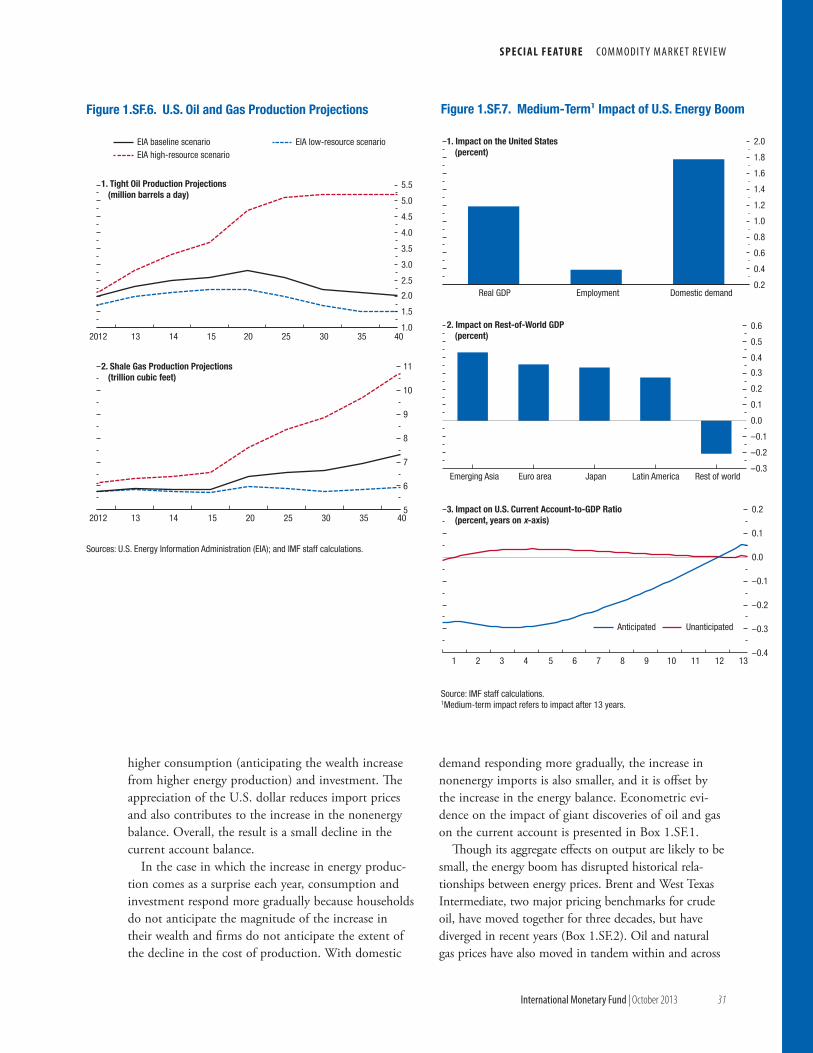
S p e c I a L F e at U r e co m m o d i t y ma r k e t r e v i e w
international monetary Fund | October 2013 31
higher consumption (anticipating the wealth increase from higher energy production) and investment. The appreciation of the U.S. dollar reduces import prices and also contributes to the increase in the nonenergy balance. Overall, the result is a small decline in the current account balance.
In the case in which the increase in energy produc-tion comes as a surprise each year, consumption and investment respond more gradually because households do not anticipate the magnitude of the increase in their wealth and firms do not anticipate the extent of the decline in the cost of production. With domestic
demand responding more gradually, the increase in nonenergy imports is also smaller, and it is offset by the increase in the energy balance. Econometric evi-dence on the impact of giant discoveries of oil and gas on the current account is presented in Box 1.SF.1.
Though its aggregate effects on output are likely to be small, the energy boom has disrupted historical rela-tionships between energy prices. Brent and West Texas Intermediate, two major pricing benchmarks for crude oil, have moved together for three decades, but have diverged in recent years (Box 1.SF.2). Oil and natural gas prices have also moved in tandem within and across
5
6
7
8
9
10
11
2012 13 14 15 20 25 30 35 40
1.0
1.5
2.0
2.5
3.0
3.5
4.0
4.5
5.0
5.5
2012 13 14 15 20 25 30 35 40
Sources: U.S. Energy Information Administration (EIA); and IMF staff calculations.
Figure 1.SF.6. U.S. Oil and Gas Production Projections
EIA baseline scenario EIA low-resource scenarioEIA high-resource scenario
1. Tight Oil Production Projections(million barrels a day)
2. Shale Gas Production Projections(trillion cubic feet)
0.2
0.4
0.6
0.8
1.0
1.2
1.4
1.6
1.8
2.0
Real GDP Employment Domestic demand
Source: IMF staff calculations. 1Medium-term impact refers to impact after 13 years.
Figure 1.SF.7. Medium-Term1 Impact of U.S. Energy Boom
–0.3
–0.2
–0.1
0.0
0.1
0.2
0.3
0.4
0.5
0.6
Emerging Asia Euro area Japan Latin America Rest of world
1. Impact on the United States (percent)
2. Impact on Rest-of-World GDP (percent)
–0.4
–0.3
–0.2
–0.1
0.0
0.1
0.2
1 2 3 4 5 6 7 8 9 10 11 12 13
3. Impact on U.S. Current Account-to-GDP Ratio (percent, years on x-axis)
Anticipated Unanticipated
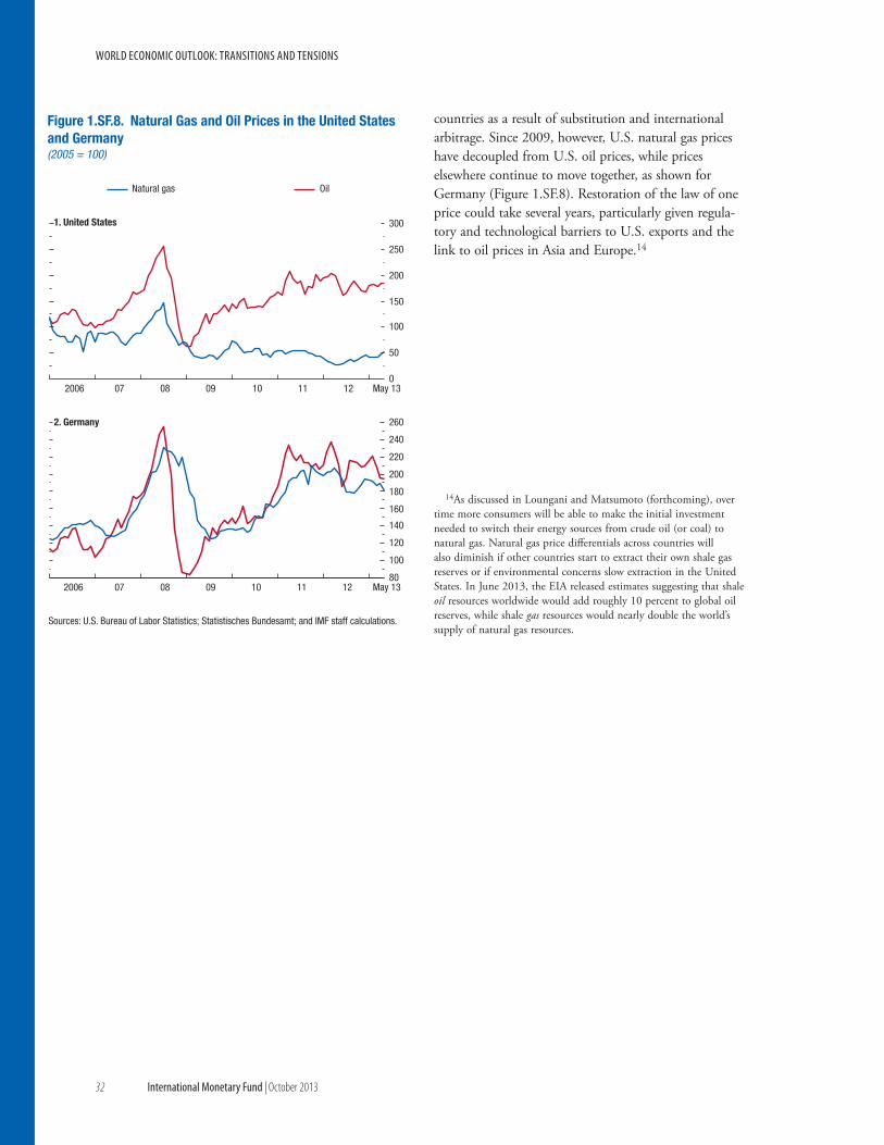
world economic outlook: transitions and tensions
32 international monetary Fund | October 2013
countries as a result of substitution and international arbitrage. Since 2009, however, U.S. natural gas prices have decoupled from U.S. oil prices, while prices elsewhere continue to move together, as shown for Germany (Figure 1.SF.8). Restoration of the law of one price could take several years, particularly given regula-tory and technological barriers to U.S. exports and the link to oil prices in Asia and Europe.14
14As discussed in Loungani and Matsumoto (forthcoming), over time more consumers will be able to make the initial investment needed to switch their energy sources from crude oil (or coal) to natural gas. Natural gas price differentials across countries will also diminish if other countries start to extract their own shale gas reserves or if environmental concerns slow extraction in the United States. In June 2013, the EIA released estimates suggesting that shale oil resources worldwide would add roughly 10 percent to global oil reserves, while shale gas resources would nearly double the world’s supply of natural gas resources.
0
50
100
150
200
250
300
2006 07 08 09 10 11 12 May 13
Sources: U.S. Bureau of Labor Statistics; Statistisches Bundesamt; and IMF staff calculations.
Figure 1.SF.8. Natural Gas and Oil Prices in the United Statesand Germany(2005 = 100)
Natural gas Oil
80
100
120
140
160
180
200
220
240
260
2006 07 08 09 10 11 12 May 13
1. United States
2. Germany

S p e c I a L F e at U r e co m m o d i t y ma r k e t r e v i e w
international monetary Fund | October 2013 33
Discoveries of giant oil and gas fields—fields contain-ing ultimate recoverable reserves equivalent to at least 500 million barrels—have been relatively widespread across countries since the 1970s. These discoveries constitute a unique source of exogenous future income shocks. Regression results, using a panel of 178 countries over the period 1970 to 2012, show that the effect of these discoveries was first to decrease the cur-rent account balance and then to increase it before the effect leveled off (Figure 1.SF.1.1).1 Hence, the pattern of the effect is similar to the case of the unanticipated increase in energy production shown in IMF Global Economic Model (GEM) simulations. The regression estimates imply that a discovery equal to the size of proven reserves in U.S. unconventional energy in the United States would lead at its peak to about a 0.1 percent of GDP increase in the U.S. current account balance.
The effect thus is small, as also suggested by the GEM simulations. There are cases in which oil and gas discoveries have had larger effects on the cur-rent account, but the size of those discoveries was larger than the expected increase in the case of the United States. For instance, the share of North Sea oil discoveries in U.K. GDP was about 6 to 7 percent at its peak. After initially moving in line with the sharp increase and decline in oil revenues, the U.K. current account decoupled from oil revenues, which have remained low and stable at about 1½ percent of GDP since 1990. The impact on the current account was larger in Norway because of the much larger share of the gas and oil extraction sector in the economy—nearly 25 percent—and the country’s fiscal policy of keeping most of the oil revenues in a special fund.
The author of this box is Rabah Arezki.1Details are given in Arezki and Sheng (forthcoming).
Box 1.SF.1. energy Booms and the current account: cross-country experience
Figure 1.SF.1.1. Giant Oil and GasDiscoveries and the Current Account
Source: IMF staff calculations.
10
20
30
40
50
60
70
80
90
1970s 1980s 1990s 2000s 2010–12
1. Discoveries(oil and gas field discoveries, by year)
2. Oil Discoveries and Current Account(years after discovery, regression coefficient)
–0.06
–0.04
–0.02
0.00
0.02
0.04
0.06
0.08
–2 0 2 4 6 8 10 12 14 16 18 20
Coefficient Confidence interval
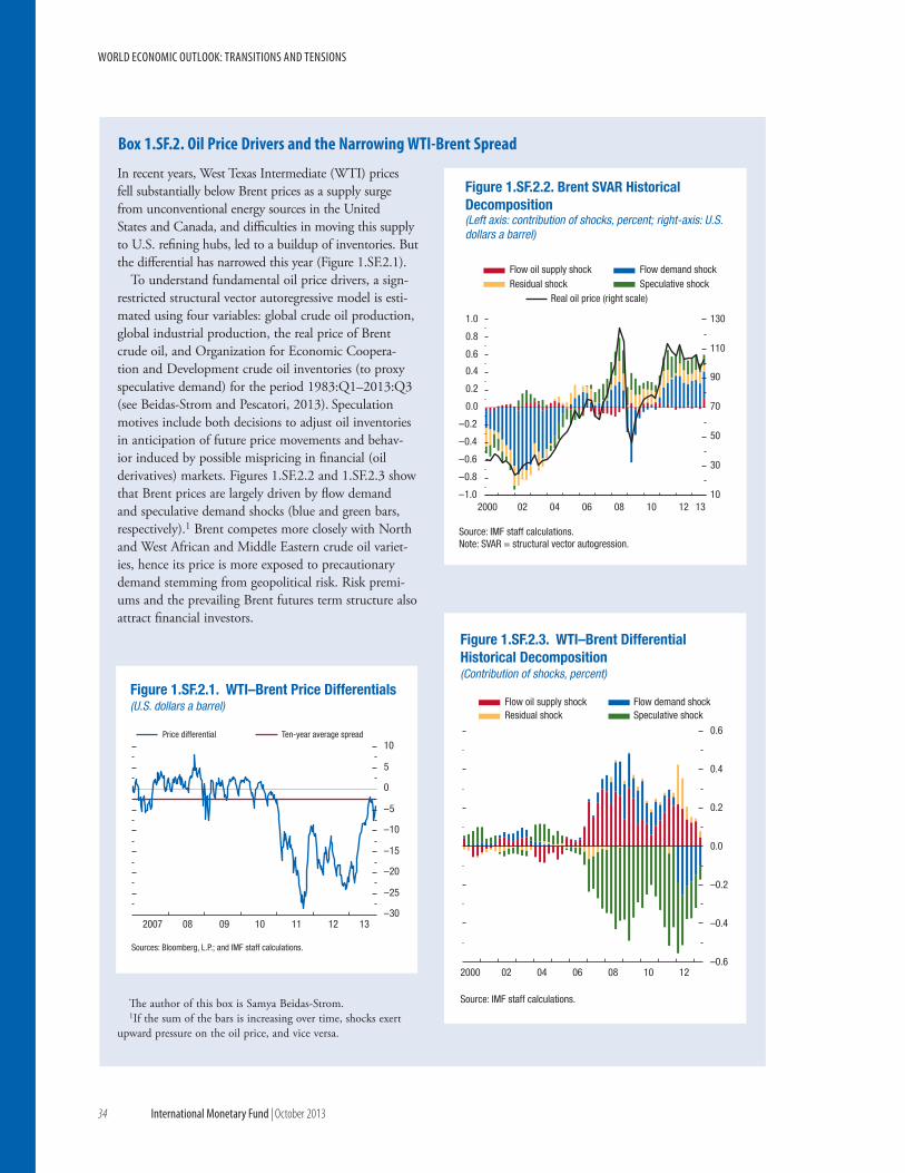
world economic outlook: transitions and tensions
34 international monetary Fund | October 2013
In recent years, West Texas Intermediate (WTI) prices fell substantially below Brent prices as a supply surge from unconventional energy sources in the United States and Canada, and difficulties in moving this supply to U.S. refining hubs, led to a buildup of inventories. But the differential has narrowed this year (Figure 1.SF.2.1).
To understand fundamental oil price drivers, a sign-restricted structural vector autoregressive model is esti-mated using four variables: global crude oil production, global industrial production, the real price of Brent crude oil, and Organization for Economic Coopera-tion and Development crude oil inventories (to proxy speculative demand) for the period 1983:Q1–2013:Q3 (see Beidas-Strom and Pescatori, 2013). Speculation motives include both decisions to adjust oil inventories in anticipation of future price movements and behav-ior induced by possible mispricing in financial (oil derivatives) markets. Figures 1.SF.2.2 and 1.SF.2.3 show that Brent prices are largely driven by flow demand and speculative demand shocks (blue and green bars, respectively).1 Brent competes more closely with North and West African and Middle Eastern crude oil variet-ies, hence its price is more exposed to precautionary demand stemming from geopolitical risk. Risk premi-ums and the prevailing Brent futures term structure also attract financial investors.
The author of this box is Samya Beidas-Strom.1If the sum of the bars is increasing over time, shocks exert
upward pressure on the oil price, and vice versa.
Box 1.SF.2. Oil price Drivers and the Narrowing WtI-Brent Spread
Figure 1.SF.2.1. WTI–Brent Price Differentials(U.S. dollars a barrel)
–30
–25
–20
–15
–10
–5
0
5
10
2007 08 09 10 11 12 13
Sources: Bloomberg, L.P.; and IMF staff calculations.
Price differential Ten-year average spread
Figure 1.SF.2.3. WTI–Brent Differential Historical Decomposition(Contribution of shocks, percent)
–0.6
–0.4
–0.2
0.0
0.2
0.4
0.6
2000 02 04 06 08 10 12
Source: IMF staff calculations.
Flow oil supply shock Flow demand shockResidual shock Speculative shock
Figure 1.SF.2.2. Brent SVAR HistoricalDecomposition(Left axis: contribution of shocks, percent; right-axis: U.S.dollars a barrel)
–1.0
–0.8
–0.6
–0.4
–0.2
0.0
0.2
0.4
0.6
0.8
1.0
10
30
50
70
90
110
130
2000 02 04 06 08 10 12 13
Source: IMF staff calculations. Note: SVAR = structural vector autogression.
Real oil price (right scale)
Flow oil supply shock Flow demand shockResidual shock Speculative shock
S p e c I a L F e at U r e co m m o d i t y ma r k e t r e v i e w
international monetary Fund | October 2013 35
Box 1.SF.2 (continued)
Replacing Brent with WTI prices, the model sug-gests that before 2007 the drivers of the two leading benchmark prices are almost identical. However, since 2007, WTI prices have been influenced more by global supply conditions (burgundy bars)—particu-larly the boom in North American supply and crude oil transportation constraints since 2009—and less by speculative demand. More recently, infrastructure bottlenecks have eased (yellow bars) and speculative
and seasonal demand increased, raising WTI and nar-rowing the spread. But this narrowing may not prove durable. Seasonal U.S. demand will dissipate in the third quarter, and sufficient crude oil infrastructure to carry oil from the middle of the United States to the Gulf coast will not be reconfigured and completed until late next year. Therefore, downward pressure on WTI could continue, altering the WTI futures term structure and lowering recent investor interest.
world economic outlook: transitions and tensions
36 international monetary Fund | October 2013
The U.S. Federal Reserve’s communication in late May about a future tapering of asset purchases appears to have been a wake-up call to markets that the excep-tionally accommodative U.S. monetary policy could soon reach a turning point. By August, U.S. 10-year yields had risen by more than 80 basis points, and many emerging markets experienced capital outflows, higher bond yields, and lower equity prices, which were partly offset by some exchange rate deprecia-tion (see the main text of the chapter). Bond yields declined modestly after the Federal Reserve recently communicated its decision not yet to begin tapering of asset purchases, but they still remain above pre-taper-talk levels.
A key question is how markets will respond when U.S. monetary stimulus is eventually withdrawn. This box sheds light on the question by drawing on previ-ous turning points in U.S. monetary policy since 1990 and assessing whether the consequences for emerging markets may be different this time.1
The analysis indicates that no broad-based dete-rioration in global economic and financial health occurred at the onset of previous episodes of U.S. monetary policy tightening since 1990. Each of the three previous episodes of sustained U.S. federal funds rate hikes—starting in February 1994, June 1999, and June 2004—was motivated by strong economic growth. The international consequences were limited in 1999 and 2004, and global growth continued to be strong. However, the 1994 episode was followed by deteriorating financial conditions in emerging market economies—reflecting some ongoing crises and preexisting imbalances that widened further in the context of fixed exchange rates after interest rates rose globally—and some crises and recessions afterward.
The analysis also suggests that the recent tighten-ing in global financial markets was not exceptional by historical standards. Even in previous episodes, long-term U.S. bond yields rose before policy rates were raised, in anticipation of stronger economic
The authors of this box are Michal Andrle and Rupa Duttagupta, with support from Shan Chen, Serhat Solmaz, and Bennet Voorhees.
1The stylized facts presented here are associations between various indicators and a tight U.S. monetary policy stance and should not be interpreted as the causal effect of the latter on the former. For an identification of the causal effects of a rise in U.S. interest rates, see Chapter 3 of this World Economic Outlook (WEO) and Chapter 4 of the April 2011 WEO.
conditions and tighter monetary policy. Still, some similarities between the current and the 1994 episode are a concern. Both involved large capital inflows to emerging market economies prior to the event, cyclical divergences between the U.S. and emerging market economies, and marked declines in equity prices and increases in long-term bonds yields at the onset of the event. However, policy frameworks in emerging market economies are stronger today, with greater exchange rate flexibility and higher foreign exchange reserve buffers. They should, thus, be better prepared to weather a tightening in external financing.
Historical turning points in U.S. monetary policy
This box focuses on the post-1990s period, when U.S. inflation was relatively low and stable, and identifies three distinct phases of U.S. monetary policy tighten-ing (Figure 1.1.1):2 • February 1994 to July 1995: The federal funds rate,
which had been held constant for more than a year, was raised on February 4, 1994, motivated partly by a stronger-than-expected pace of growth of the U.S. economy.3 Rates were raised by a cumulative 300 basis points within 12 months, to 6 percent from 3 percent. Long-term yields (on 10-year Treasuries) rose sharply until late 1994 but declined thereafter, given stabilized inflation expectations.
• June 1999 to December 2000: After continuous rate cuts since the second half of 1998, the first rate hike in the next tightening phase occurred on June 30, 1999. The policy rate was raised by 175 basis points during the next 19 months, to 6.5 percent from 4.75 percent. Long-term yields rose at a slower pace than in 1994 and began declining after six months.
• June 2004 to August 2007: The policy rate was raised on June 30, 2004, after rate cuts throughout the previous three years, and gradually increased during the next three years, to 5.25 percent from
2The following criteria are used to identify a tightening phase in U.S. monetary policy: the federal funds target rate is raised after at least six months of unchanged or declining rates, fol-lowed by increases for at least six months. Figures 1.1.1, 1.1.2, and 1.1.3 trace the evolution of alternative indicators in the months (quarters) before and after the month (quarter) of the monetary policy turning point.
3Inflation was maintained at below 3 percent during this period, and the move to announce the intended federal funds rate established greater credibility and transparency in the policy framework (see Goodfriend, 2003).
Box 1.1. taper talks: What to expect when the United States Is tightening
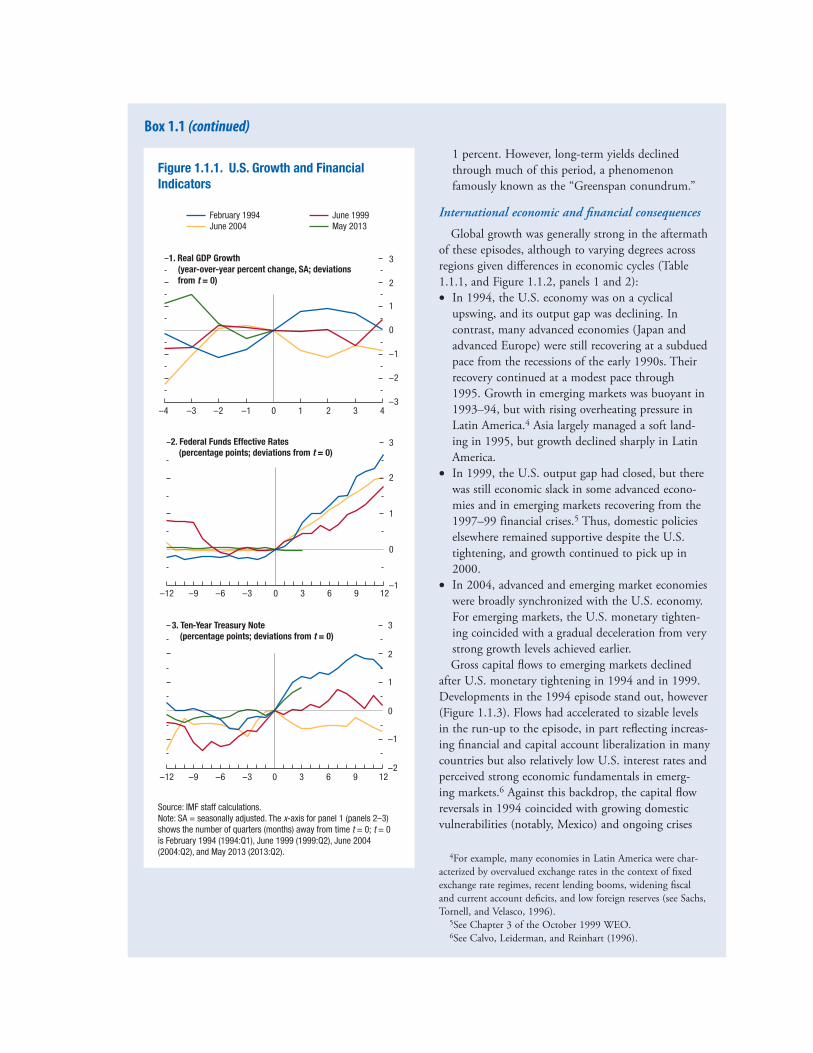
1 percent. However, long-term yields declined through much of this period, a phenomenon famously known as the “Greenspan conundrum.”
International economic and financial consequences
Global growth was generally strong in the aftermath of these episodes, although to varying degrees across regions given differences in economic cycles (Table 1.1.1, and Figure 1.1.2, panels 1 and 2): • In 1994, the U.S. economy was on a cyclical
upswing, and its output gap was declining. In contrast, many advanced economies (Japan and advanced Europe) were still recovering at a subdued pace from the recessions of the early 1990s. Their recovery continued at a modest pace through 1995. Growth in emerging markets was buoyant in 1993–94, but with rising overheating pressure in Latin America.4 Asia largely managed a soft land-ing in 1995, but growth declined sharply in Latin America.
• In 1999, the U.S. output gap had closed, but there was still economic slack in some advanced econo-mies and in emerging markets recovering from the 1997–99 financial crises.5 Thus, domestic policies elsewhere remained supportive despite the U.S. tightening, and growth continued to pick up in 2000.
• In 2004, advanced and emerging market economies were broadly synchronized with the U.S. economy. For emerging markets, the U.S. monetary tighten-ing coincided with a gradual deceleration from very strong growth levels achieved earlier.Gross capital flows to emerging markets declined
after U.S. monetary tightening in 1994 and in 1999. Developments in the 1994 episode stand out, however (Figure 1.1.3). Flows had accelerated to sizable levels in the run-up to the episode, in part reflecting increas-ing financial and capital account liberalization in many countries but also relatively low U.S. interest rates and perceived strong economic fundamentals in emerg-ing markets.6 Against this backdrop, the capital flow reversals in 1994 coincided with growing domestic vulnerabilities (notably, Mexico) and ongoing crises
4For example, many economies in Latin America were char-acterized by overvalued exchange rates in the context of fixed exchange rate regimes, recent lending booms, widening fiscal and current account deficits, and low foreign reserves (see Sachs, Tornell, and Velasco, 1996).
5See Chapter 3 of the October 1999 WEO.6See Calvo, Leiderman, and Reinhart (1996).
Box 1.1 (continued)
Figure 1.1.1. U.S. Growth and FinancialIndicators
–3
–2
–1
0
1
2
3
–4 –3 –2 –1 0 1 2 3 4
1. Real GDP Growth (year-over-year percent change, SA; deviations from t = 0)
February 1994 June 1999June 2004 May 2013
–1
0
1
2
3
–12 –9 –6 –3 0 3 6 9 12
2. Federal Funds Effective Rates(percentage points; deviations from t = 0)
–2
–1
0
1
2
3
–12 –9 –6 –3 0 3 6 9 12
3. Ten-Year Treasury Note (percentage points; deviations from t = 0)
Source: IMF staff calculations.Note: SA = seasonally adjusted. The x-axis for panel 1 (panels 2–3) shows the number of quarters (months) away from time t = 0; t = 0 is February 1994 (1994:Q1), June 1999 (1999:Q2), June 2004 (2004:Q2), and May 2013 (2013:Q2).
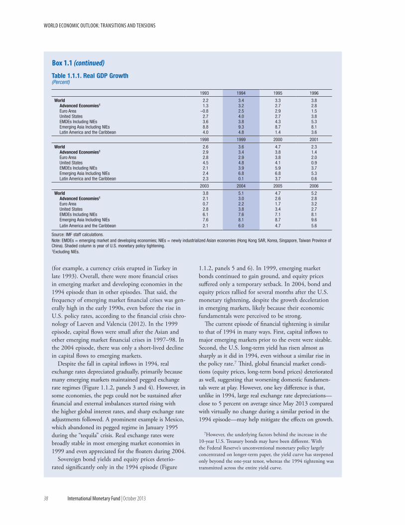
world economic outlook: transitions and tensions
38 international monetary Fund | October 2013
(for example, a currency crisis erupted in Turkey in late 1993). Overall, there were more financial crises in emerging market and developing economies in the 1994 episode than in other episodes. That said, the frequency of emerging market financial crises was gen-erally high in the early 1990s, even before the rise in U.S. policy rates, according to the financial crisis chro-nology of Laeven and Valencia (2012). In the 1999 episode, capital flows were small after the Asian and other emerging market financial crises in 1997–98. In the 2004 episode, there was only a short-lived decline in capital flows to emerging markets.
Despite the fall in capital inflows in 1994, real exchange rates depreciated gradually, primarily because many emerging markets maintained pegged exchange rate regimes (Figure 1.1.2, panels 3 and 4). However, in some economies, the pegs could not be sustained after financial and external imbalances started rising with the higher global interest rates, and sharp exchange rate adjustments followed. A prominent example is Mexico, which abandoned its pegged regime in January 1995 during the “tequila” crisis. Real exchange rates were broadly stable in most emerging market economies in 1999 and even appreciated for the floaters during 2004.
Sovereign bond yields and equity prices deterio-rated significantly only in the 1994 episode (Figure
1.1.2, panels 5 and 6). In 1999, emerging market bonds continued to gain ground, and equity prices suffered only a temporary setback. In 2004, bond and equity prices rallied for several months after the U.S. monetary tightening, despite the growth deceleration in emerging markets, likely because their economic fundamentals were perceived to be strong.
The current episode of financial tightening is similar to that of 1994 in many ways. First, capital inflows to major emerging markets prior to the event were sizable. Second, the U.S. long-term yield has risen almost as sharply as it did in 1994, even without a similar rise in the policy rate.7 Third, global financial market condi-tions (equity prices, long-term bond prices) deteriorated as well, suggesting that worsening domestic fundamen-tals were at play. However, one key difference is that, unlike in 1994, large real exchange rate depreciations—close to 5 percent on average since May 2013 compared with virtually no change during a similar period in the 1994 episode—may help mitigate the effects on growth.
7However, the underlying factors behind the increase in the 10-year U.S. Treasury bonds may have been different. With the Federal Reserve’s unconventional monetary policy largely concentrated on longer-term paper, the yield curve has steepened only beyond the one-year tenor, whereas the 1994 tightening was transmitted across the entire yield curve.
Box 1.1 (continued)
Table 1.1.1. Real GDP Growth(Percent)
1993 1994 1995 1996
World 2.2 3.4 3.3 3.8Advanced Economies1 1.3 3.2 2.7 2.8Euro Area –0.8 2.5 2.9 1.5United States 2.7 4.0 2.7 3.8EMDEs Including NIEs 3.6 3.8 4.3 5.3Emerging Asia Including NIEs 8.8 9.3 8.7 8.1Latin America and the Caribbean 4.0 4.8 1.4 3.6
1998 1999 2000 2001
World 2.6 3.6 4.7 2.3Advanced Economies1 2.9 3.4 3.8 1.4Euro Area 2.8 2.9 3.8 2.0United States 4.5 4.8 4.1 0.9EMDEs Including NIEs 2.1 3.9 5.9 3.7Emerging Asia Including NIEs 2.4 6.8 6.8 5.3Latin America and the Caribbean 2.3 0.1 3.7 0.6
2003 2004 2005 2006
World 3.8 5.1 4.7 5.2Advanced Economies1 2.1 3.0 2.6 2.8Euro Area 0.7 2.2 1.7 3.2United States 2.8 3.8 3.4 2.7EMDEs Including NIEs 6.1 7.6 7.1 8.1Emerging Asia Including NIEs 7.6 8.1 8.7 9.6Latin America and the Caribbean 2.1 6.0 4.7 5.6
Source: IMF staff calculations.Note: EMDEs = emerging market and developing economies; NIEs = newly industrialized Asian economies (Hong Kong SAR, Korea, Singapore, Taiwan Province of China). Shaded column is year of U.S. monetary policy tightening.1Excluding NIEs.
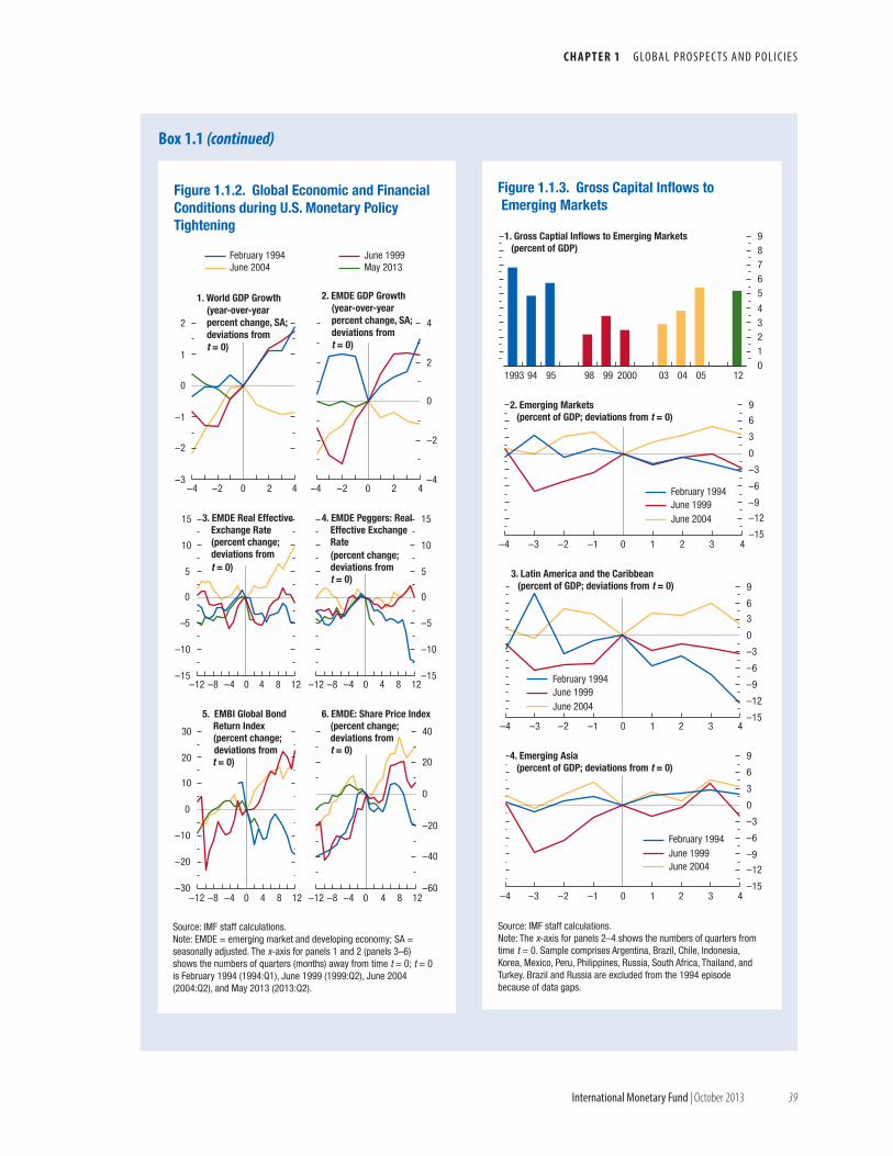
c h a p t e r 1 G lo b a l P r o s P e c ts a n d P o l i c i e s
international monetary Fund | October 2013 39
Box 1.1 (continued)
–15
–12
–9
–6
–3
0
3
6
9
–4 –3 –2 –1 0 1 2 3 4
Figure 1.1.3. Gross Capital Inflows to Emerging Markets
–15
–12
–9
–6
–3
0
3
6
9
–4 –3 –2 –1 0 1 2 3 4
2. Emerging Markets(percent of GDP; deviations from t = 0)
February 1994June 1999June 2004
–15
–12
–9
–6
–3
0
3
6
9
–4 –3 –2 –1 0 1 2 3 4
3. Latin America and the Caribbean(percent of GDP; deviations from t = 0)
4. Emerging Asia(percent of GDP; deviations from t = 0)
February 1994June 1999June 2004
February 1994June 1999June 2004
01234
56789
1993 94 95 98 99 2000 03 04 05 12
1. Gross Captial Inflows to Emerging Markets(percent of GDP)
Source: IMF staff calculations.Note: The x-axis for panels 2–4 shows the numbers of quarters from time t = 0. Sample comprises Argentina, Brazil, Chile, Indonesia, Korea, Mexico, Peru, Philippines, Russia, South Africa, Thailand, and Turkey. Brazil and Russia are excluded from the 1994 episode because of data gaps.
Figure 1.1.2. Global Economic and FinancialConditions during U.S. Monetary PolicyTightening
–3
–2
–1
0
1
2
–4 –2 0 2 4
1. World GDP Growth (year-over-year percent change, SA; deviations from t = 0)
February 1994 June 1999June 2004 May 2013
–4
–2
0
2
4
–4 –2 0 2 4
2. EMDE GDP Growth (year-over-year percent change, SA; deviations from t = 0)
–15
–10
–5
0
5
10
15
–12 –8 –4 0 4 8 12
3. EMDE Real EffectiveExchange Rate(percent change;deviations from t = 0)
–15
–10
–5
0
5
10
15
–12 –8 –4 0 4 8 12
4. EMDE Peggers: Real Effective Exchange Rate(percent change;deviations from t = 0)
–30
–20
–10
0
10
20
30
–12 –8 –4 0 4 8 12
5. EMBI Global BondReturn Index (percent change;deviations fromt = 0)
–60
–40
–20
0
20
40
–12 –8 –4 0 4 8 12
6. EMDE: Share Price Index(percent change;deviations fromt = 0)
Source: IMF staff calculations.Note: EMDE = emerging market and developing economy; SA = seasonally adjusted. The x-axis for panels 1 and 2 (panels 3–6) shows the numbers of quarters (months) away from time t = 0; t = 0 is February 1994 (1994:Q1), June 1999 (1999:Q2), June 2004 (2004:Q2), and May 2013 (2013:Q2).
world economic outlook: transitions and tensions
40 international monetary Fund | October 2013
Lessons from history
• History suggests that the world economy did not fall apart in previous U.S. monetary tightening episodes. Other than for a few economies, the cross-border consequences were largely benign, and global growth continued to be strong.
• When difficulties arose, as during the 1994 episode, they typically reflected prevailing vulnerabilities that proved to be unsustainable in a changing global environment.
• The potential consequences of the eventual tight-ening of U.S. monetary policy will depend on its magnitude and pace and on how broadly the tightening affects financial conditions. For instance, although historical trends suggest that the U.S. 10-year sovereign rate would rise by more than 200 basis points to reach close to 5 percent over the medium term, the increase could be smaller if
medium-term growth and inflation in the United States do not return to historical averages. With many emerging market economies slow-
ing after a cyclical peak in 2010–11, they will need to achieve a soft landing as the external financing environment tightens. Many of them have adopted stronger policies during the past decade, have higher reserves, and flexible exchange rate regimes, although in some countries fiscal imbalances have widened in recent years (see the October 2013 Fiscal Monitor), and the share of nonresident holdings of locally issued debt has increased (see the October 2013 Global Financial Stability Report). If these economies rebuild their policy buffers while times are still good, and use their exchange rates as shock absorbers while contain-ing inflation and financial stability risks, they should be better able to endure a tightening in financial conditions than in 1994.
Box 1.1 (continued)
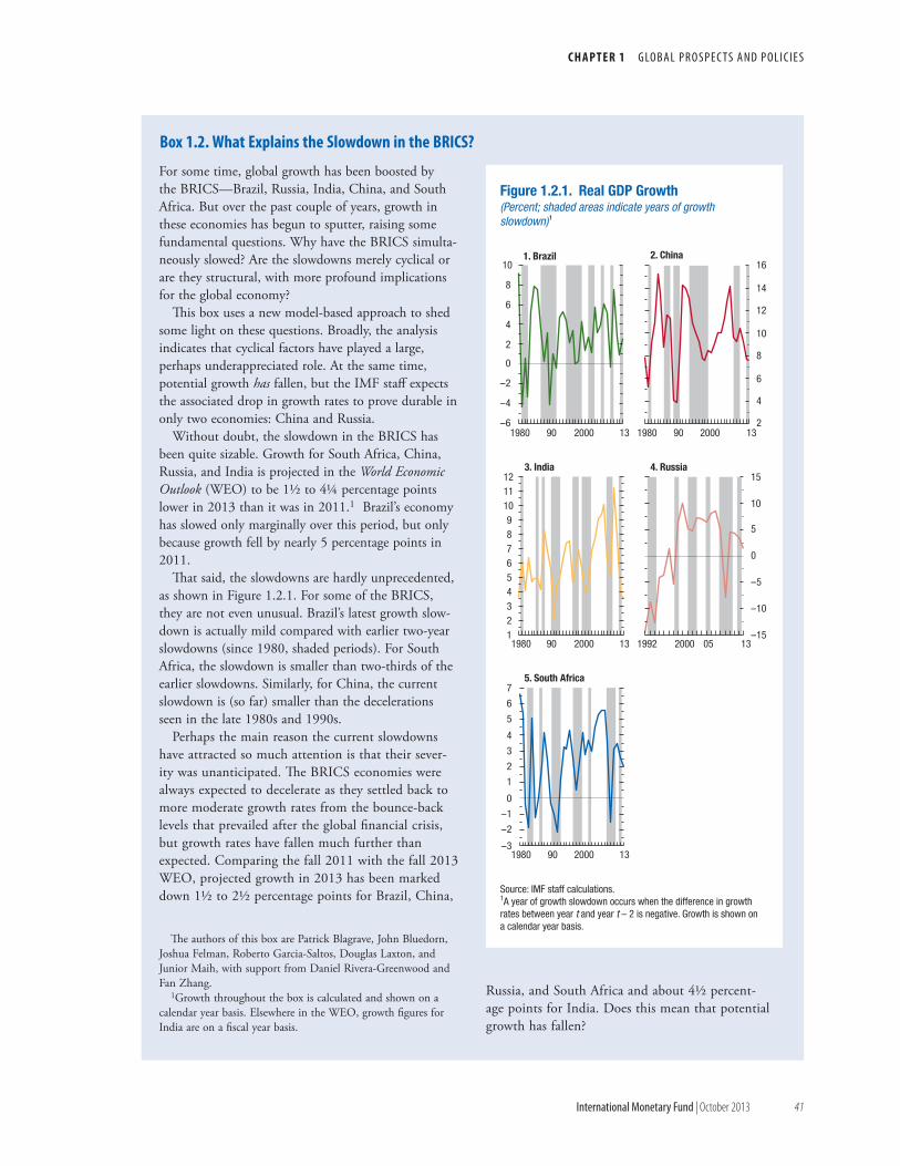
c h a p t e r 1 G lo b a l P r o s P e c ts a n d P o l i c i e s
international monetary Fund | October 2013 41
For some time, global growth has been boosted by the BRICS—Brazil, Russia, India, China, and South Africa. But over the past couple of years, growth in these economies has begun to sputter, raising some fundamental questions. Why have the BRICS simulta-neously slowed? Are the slowdowns merely cyclical or are they structural, with more profound implications for the global economy?
This box uses a new model-based approach to shed some light on these questions. Broadly, the analysis indicates that cyclical factors have played a large, perhaps underappreciated role. At the same time, potential growth has fallen, but the IMF staff expects the associated drop in growth rates to prove durable in only two economies: China and Russia.
Without doubt, the slowdown in the BRICS has been quite sizable. Growth for South Africa, China, Russia, and India is projected in the World Economic Outlook (WEO) to be 1½ to 4¼ percentage points lower in 2013 than it was in 2011.1 Brazil’s economy has slowed only marginally over this period, but only because growth fell by nearly 5 percentage points in 2011.
That said, the slowdowns are hardly unprecedented, as shown in Figure 1.2.1. For some of the BRICS, they are not even unusual. Brazil’s latest growth slow-down is actually mild compared with earlier two-year slowdowns (since 1980, shaded periods). For South Africa, the slowdown is smaller than two-thirds of the earlier slowdowns. Similarly, for China, the current slowdown is (so far) smaller than the decelerations seen in the late 1980s and 1990s.
Perhaps the main reason the current slowdowns have attracted so much attention is that their sever-ity was unanticipated. The BRICS economies were always expected to decelerate as they settled back to more moderate growth rates from the bounce-back levels that prevailed after the global financial crisis, but growth rates have fallen much further than expected. Comparing the fall 2011 with the fall 2013 WEO, projected growth in 2013 has been marked down 1½ to 2½ percentage points for Brazil, China,
The authors of this box are Patrick Blagrave, John Bluedorn, Joshua Felman, Roberto Garcia-Saltos, Douglas Laxton, and Junior Maih, with support from Daniel Rivera-Greenwood and Fan Zhang.
1Growth throughout the box is calculated and shown on a calendar year basis. Elsewhere in the WEO, growth figures for India are on a fiscal year basis.
Russia, and South Africa and about 4½ percent-age points for India. Does this mean that potential growth has fallen?
Box 1.2. What explains the Slowdown in the BrIcS?
Figure 1.2.1. Real GDP Growth(Percent; shaded areas indicate years of growthslowdown)1
–6
–4
–2
0
2
4
6
8
10
1980 90 2000 13
1. Brazil
2
4
6
8
10
12
14
16
1980 90 2000 13
2. China
123456789
101112
1980 90 2000 13
3. India
–15
–10
–5
0
5
10
15
1992 2000 05 13
4. Russia
–3
–2
–1
0
1
2
3
4
5
6
7
1980 90 2000 13
5. South Africa
Source: IMF staff calculations.1A year of growth slowdown occurs when the difference in growth rates between year t and year t – 2 is negative. Growth is shown on a calendar year basis.
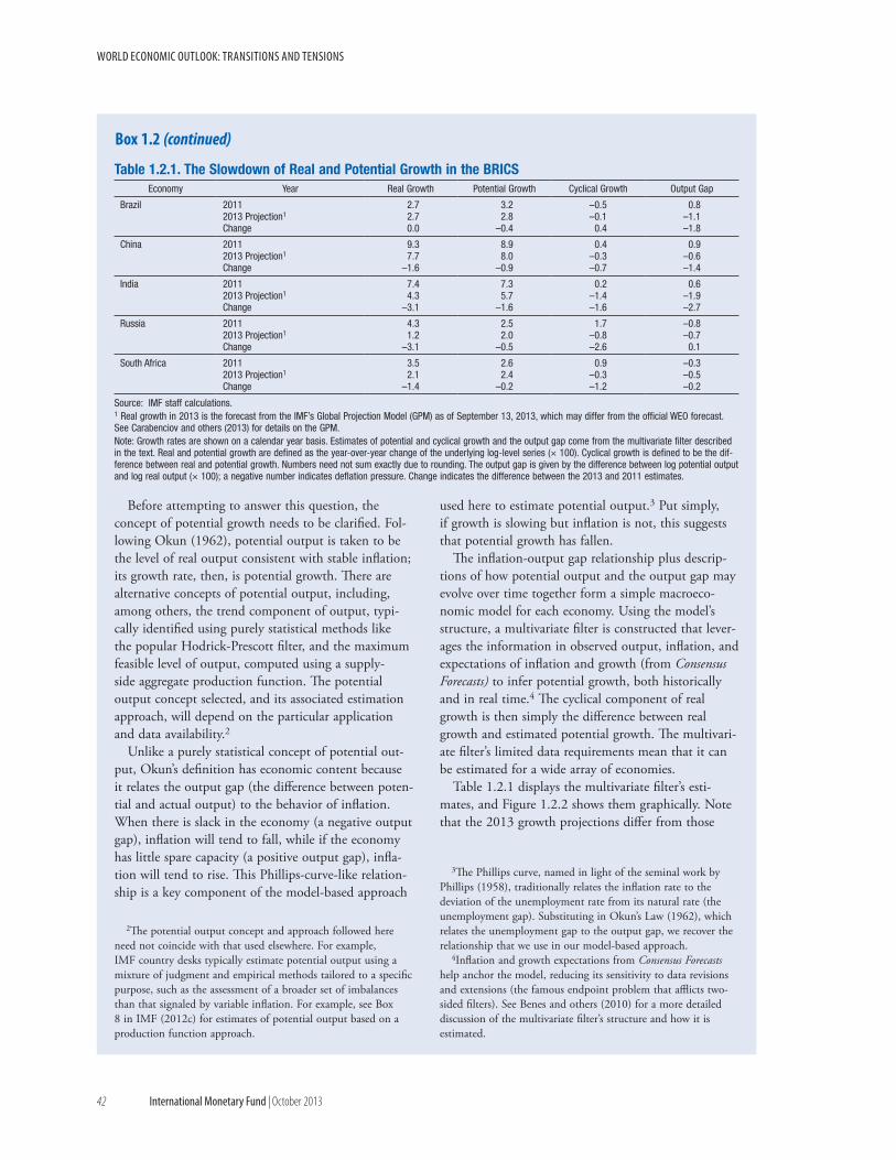
world economic outlook: transitions and tensions
42 international monetary Fund | October 2013
Before attempting to answer this question, the concept of potential growth needs to be clarified. Fol-lowing Okun (1962), potential output is taken to be the level of real output consistent with stable inflation; its growth rate, then, is potential growth. There are alternative concepts of potential output, including, among others, the trend component of output, typi-cally identified using purely statistical methods like the popular Hodrick-Prescott filter, and the maximum feasible level of output, computed using a supply-side aggregate production function. The potential output concept selected, and its associated estimation approach, will depend on the particular application and data availability.2
Unlike a purely statistical concept of potential out-put, Okun’s definition has economic content because it relates the output gap (the difference between poten-tial and actual output) to the behavior of inflation. When there is slack in the economy (a negative output gap), inflation will tend to fall, while if the economy has little spare capacity (a positive output gap), infla-tion will tend to rise. This Phillips-curve-like relation-ship is a key component of the model-based approach
2The potential output concept and approach followed here need not coincide with that used elsewhere. For example, IMF country desks typically estimate potential output using a mixture of judgment and empirical methods tailored to a specific purpose, such as the assessment of a broader set of imbalances than that signaled by variable inflation. For example, see Box 8 in IMF (2012c) for estimates of potential output based on a production function approach.
used here to estimate potential output.3 Put simply, if growth is slowing but inflation is not, this suggests that potential growth has fallen.
The inflation-output gap relationship plus descrip-tions of how potential output and the output gap may evolve over time together form a simple macroeco-nomic model for each economy. Using the model’s structure, a multivariate filter is constructed that lever-ages the information in observed output, inflation, and expectations of inflation and growth (from Consensus Forecasts) to infer potential growth, both historically and in real time.4 The cyclical component of real growth is then simply the difference between real growth and estimated potential growth. The multivari-ate filter’s limited data requirements mean that it can be estimated for a wide array of economies.
Table 1.2.1 displays the multivariate filter’s esti-mates, and Figure 1.2.2 shows them graphically. Note that the 2013 growth projections differ from those
3The Phillips curve, named in light of the seminal work by Phillips (1958), traditionally relates the inflation rate to the deviation of the unemployment rate from its natural rate (the unemployment gap). Substituting in Okun’s Law (1962), which relates the unemployment gap to the output gap, we recover the relationship that we use in our model-based approach.
4Inflation and growth expectations from Consensus Forecasts help anchor the model, reducing its sensitivity to data revisions and extensions (the famous endpoint problem that afflicts two-sided filters). See Benes and others (2010) for a more detailed discussion of the multivariate filter’s structure and how it is estimated.
Box 1.2 (continued)
Table 1.2.1. The Slowdown of Real and Potential Growth in the BRICSEconomy Year Real Growth Potential Growth Cyclical Growth Output Gap
Brazil 2011 2.7 3.2 –0.5 0.82013 Projection1 2.7 2.8 –0.1 –1.1Change 0.0 –0.4 0.4 –1.8
China 2011 9.3 8.9 0.4 0.92013 Projection1 7.7 8.0 –0.3 –0.6Change –1.6 –0.9 –0.7 –1.4
India 2011 7.4 7.3 0.2 0.62013 Projection1 4.3 5.7 –1.4 –1.9Change –3.1 –1.6 –1.6 –2.7
Russia 2011 4.3 2.5 1.7 –0.82013 Projection1 1.2 2.0 –0.8 –0.7Change –3.1 –0.5 –2.6 0.1
South Africa 2011 3.5 2.6 0.9 –0.32013 Projection1 2.1 2.4 –0.3 –0.5Change –1.4 –0.2 –1.2 –0.2
Source: IMF staff calculations.1 Real growth in 2013 is the forecast from the IMF’s Global Projection Model (GPM) as of September 13, 2013, which may differ from the official WEO forecast. See Carabenciov and others (2013) for details on the GPM.Note: Growth rates are shown on a calendar year basis. Estimates of potential and cyclical growth and the output gap come from the multivariate filter described in the text. Real and potential growth are defined as the year-over-year change of the underlying log-level series (× 100). Cyclical growth is defined to be the dif-ference between real and potential growth. Numbers need not sum exactly due to rounding. The output gap is given by the difference between log potential output and log real output (× 100); a negative number indicates deflation pressure. Change indicates the difference between the 2013 and 2011 estimates.
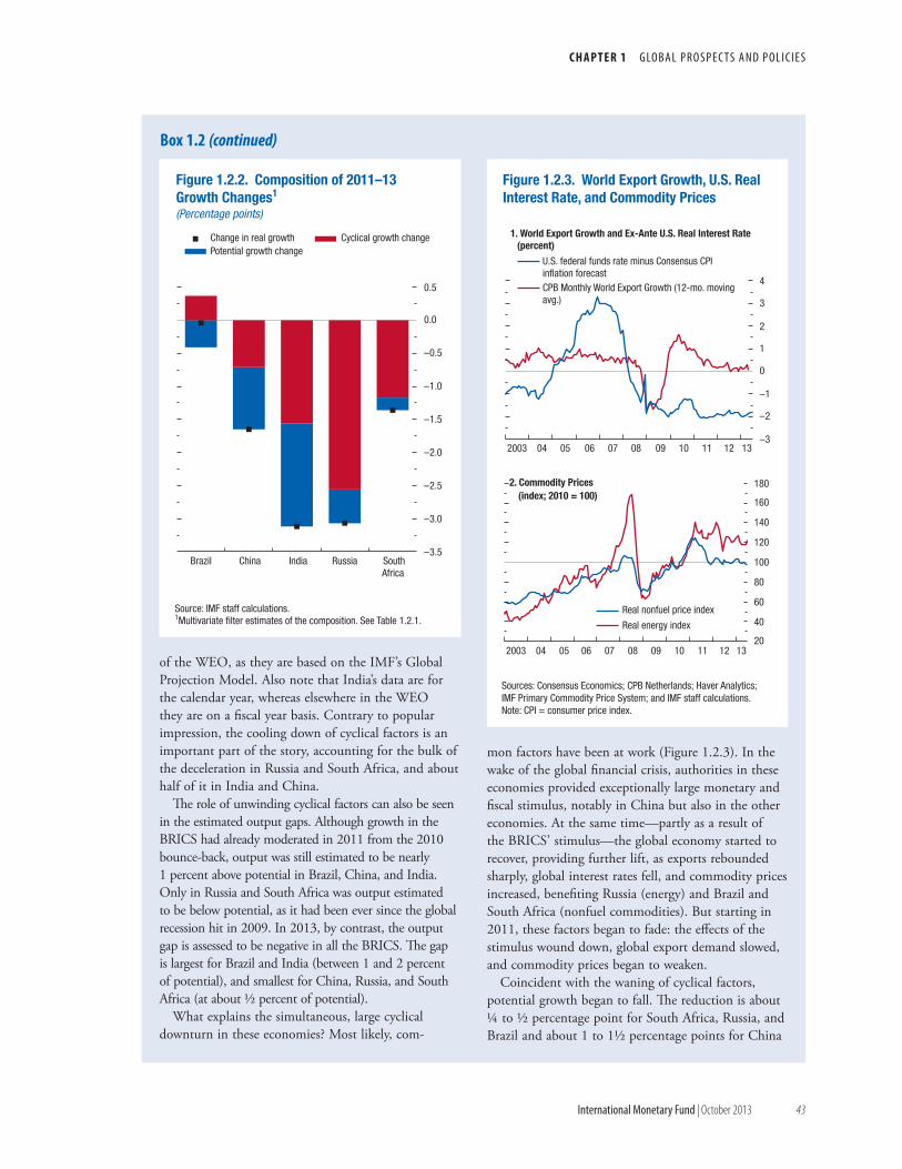
c h a p t e r 1 G lo b a l P r o s P e c ts a n d P o l i c i e s
international monetary Fund | October 2013 43
of the WEO, as they are based on the IMF’s Global Projection Model. Also note that India’s data are for the calendar year, whereas elsewhere in the WEO they are on a fiscal year basis. Contrary to popular impression, the cooling down of cyclical factors is an important part of the story, accounting for the bulk of the deceleration in Russia and South Africa, and about half of it in India and China.
The role of unwinding cyclical factors can also be seen in the estimated output gaps. Although growth in the BRICS had already moderated in 2011 from the 2010 bounce-back, output was still estimated to be nearly 1 percent above potential in Brazil, China, and India. Only in Russia and South Africa was output estimated to be below potential, as it had been ever since the global recession hit in 2009. In 2013, by contrast, the output gap is assessed to be negative in all the BRICS. The gap is largest for Brazil and India (between 1 and 2 percent of potential), and smallest for China, Russia, and South Africa (at about ½ percent of potential).
What explains the simultaneous, large cyclical downturn in these economies? Most likely, com-
mon factors have been at work (Figure 1.2.3). In the wake of the global financial crisis, authorities in these economies provided exceptionally large monetary and fiscal stimulus, notably in China but also in the other economies. At the same time—partly as a result of the BRICS’ stimulus—the global economy started to recover, providing further lift, as exports rebounded sharply, global interest rates fell, and commodity prices increased, benefiting Russia (energy) and Brazil and South Africa (nonfuel commodities). But starting in 2011, these factors began to fade: the effects of the stimulus wound down, global export demand slowed, and commodity prices began to weaken.
Coincident with the waning of cyclical factors, potential growth began to fall. The reduction is about ¼ to ½ percentage point for South Africa, Russia, and Brazil and about 1 to 1½ percentage points for China
Box 1.2 (continued)
Figure 1.2.2. Composition of 2011–13Growth Changes1
(Percentage points)
Source: IMF staff calculations.1Multivariate filter estimates of the composition. See Table 1.2.1.
–3.5
–3.0
–2.5
–2.0
–1.5
–1.0
–0.5
0.0
0.5
Brazil China India Russia South Africa
Change in real growth Cyclical growth changePotential growth change
Figure 1.2.3. World Export Growth, U.S. RealInterest Rate, and Commodity Prices
–3
–2
–1
0
1
2
3
4
2003 04 05 06 07 08 09 10 11 12 13
1. World Export Growth and Ex-Ante U.S. Real Interest Rate(percent)
2. Commodity Prices(index; 2010 = 100)
20
40
60
80
100
120
140
160
180
2003 04 05 06 07 08 09 10 11 12 13
U.S. federal funds rate minus Consensus CPI inflation forecastCPB Monthly World Export Growth (12-mo. moving avg.)
Real nonfuel price index
Real energy index
Sources: Consensus Economics; CPB Netherlands; Haver Analytics; IMF Primary Commodity Price System; and IMF staff calculations. Note: CPI = consumer price index.
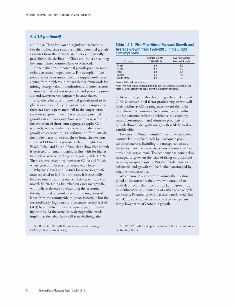
world economic outlook: transitions and tensions
44 international monetary Fund | October 2013
and India. These last two are significant reductions. For the limited time span over which potential growth estimates from the multivariate filter exist (basically, post-2000), the declines in China and India are among the largest these countries have experienced.
These reductions in potential growth point to some serious structural impediments. For example, India’s potential has been undermined by supply bottlenecks arising from problems in the regulatory framework for mining, energy, telecommunications and other sectors; a consequent slowdown in permits and project approv-als; and overstretched corporate balance sheets.
Still, the reductions in potential growth need to be placed in context. They do not necessarily imply that there has been a permanent fall in the longer-term, steady-state growth rate. That is because potential growth can and does vary from year to year, reflecting the evolution of short-term aggregate supply. Con-sequently, to assess whether the recent reductions in growth are expected to last, information from outside the model needs to be brought to bear. The five-year-ahead WEO forecasts provide such an insight. For Brazil, India, and South Africa, these show that growth is projected to remain roughly in line with (or higher than) their average of the past 15 years (Table 1.2.2). There are two exceptions, however: China and Russia, where growth is forecast to be markedly lower.
Why are China’s and Russia’s longer-term growth rates expected to fall? In both cases, it is essentially because time is running out on their current growth model. So far, China has relied on extensive growth, with policies devoted to expanding the economy through capital accumulation and the migration of labor from the countryside to urban factories.5 But the extraordinarily high rates of investment, nearly half of GDP, have resulted in excess capacity and diminish-ing returns. At the same time, demographic trends imply that the labor force will start declining after
5See Box 5 in IMF (2013h) for an analysis of the long-term challenges that China is facing.
2014, with surplus labor becoming exhausted around 2020. Moreover, total factor productivity growth will likely decline as China progresses toward the ranks of high-income countries. As a consequence, with-out fundamental reform to rebalance the economy toward consumption and stimulate productivity growth through deregulation, growth is likely to slow considerably.
The story in Russia is similar.6 For some time, the country has been held back by inadequate physi-cal infrastructure, including the transportation and electricity networks; overreliance on commodities; and a weak business climate. The economy has nonetheless managed to grow, on the back of rising oil prices and by using up spare capacity. But this model now seems exhausted, and growth will be further constrained by negative demographics.
We are now in a position to answer the question posed at the outset: is the slowdown structural or cyclical? It seems that much of the fall in growth can be attributed to an unwinding of earlier positive cycli-cal factors. Potential growth has also deteriorated. But only China and Russia are expected to have persis-tently lower rates of economic growth.
6See IMF (2012d) for deeper discussion of the structural issues confronting Russia.
Box 1.2 (continued)
Table 1.2.2. Five-Year-Ahead Forecast Growth and Average Growth from 1998–2013 in the BRICS(Percentage points)
EconomyAverage Growth
(1998–2013)Five-Year-AheadForecast Growth
Brazil 2.9 3.5China 9.6 7.0India 6.9 6.7Russia 4.4 3.5South Africa 3.2 3.5
Source: IMF staff calculations.Note: Five-year-ahead forecast growth is from the October 2013 WEO (esti-mate for 2018 growth; for India, shown on a fiscal year basis).
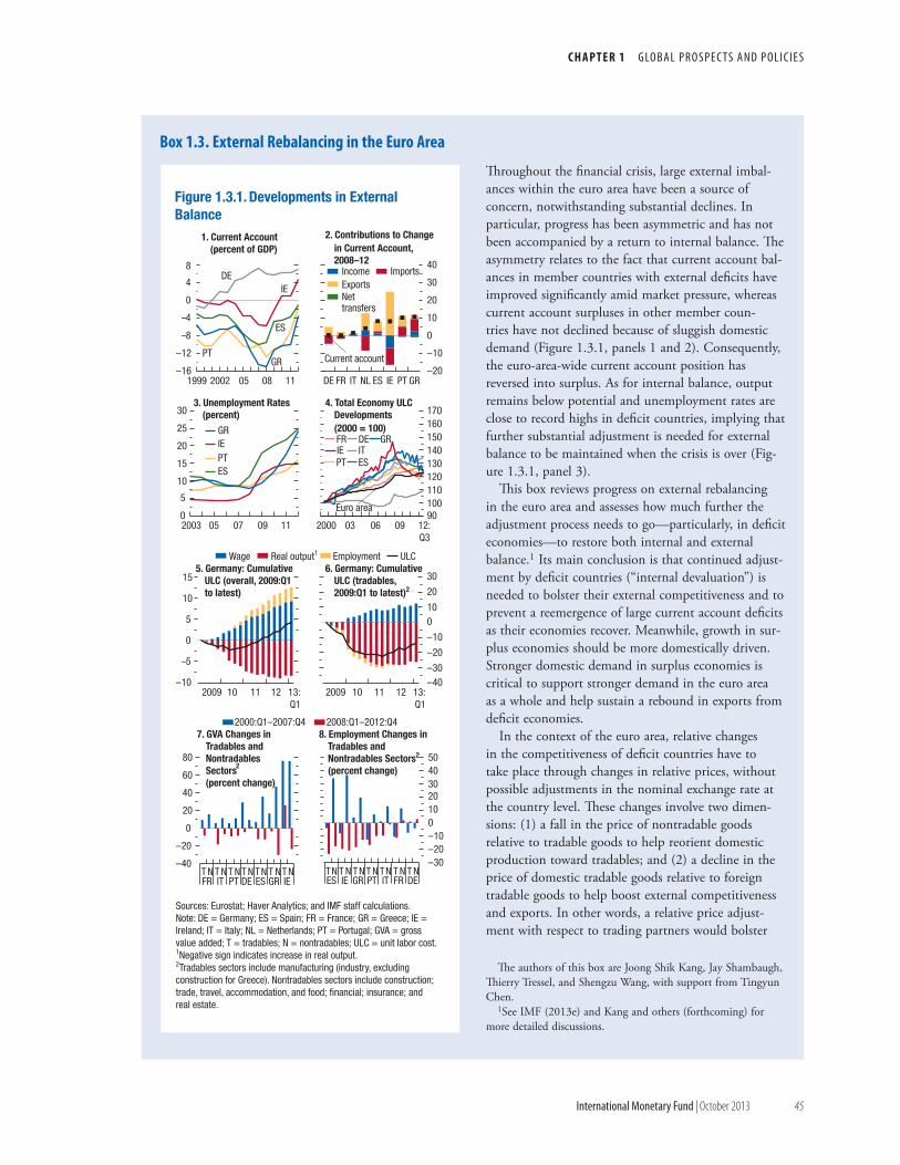
c h a p t e r 1 G lo b a l P r o s P e c ts a n d P o l i c i e s
international monetary Fund | October 2013 45
Throughout the financial crisis, large external imbal-ances within the euro area have been a source of concern, notwithstanding substantial declines. In particular, progress has been asymmetric and has not been accompanied by a return to internal balance. The asymmetry relates to the fact that current account bal-ances in member countries with external deficits have improved significantly amid market pressure, whereas current account surpluses in other member coun-tries have not declined because of sluggish domestic demand (Figure 1.3.1, panels 1 and 2). Consequently, the euro-area-wide current account position has reversed into surplus. As for internal balance, output remains below potential and unemployment rates are close to record highs in deficit countries, implying that further substantial adjustment is needed for external balance to be maintained when the crisis is over (Fig-ure 1.3.1, panel 3).
This box reviews progress on external rebalancing in the euro area and assesses how much further the adjustment process needs to go—particularly, in deficit economies—to restore both internal and external balance.1 Its main conclusion is that continued adjust-ment by deficit countries (“internal devaluation”) is needed to bolster their external competitiveness and to prevent a reemergence of large current account deficits as their economies recover. Meanwhile, growth in sur-plus economies should be more domestically driven. Stronger domestic demand in surplus economies is critical to support stronger demand in the euro area as a whole and help sustain a rebound in exports from deficit economies.
In the context of the euro area, relative changes in the competitiveness of deficit countries have to take place through changes in relative prices, without possible adjustments in the nominal exchange rate at the country level. These changes involve two dimen-sions: (1) a fall in the price of nontradable goods relative to tradable goods to help reorient domestic production toward tradables; and (2) a decline in the price of domestic tradable goods relative to foreign tradable goods to help boost external competitiveness and exports. In other words, a relative price adjust-ment with respect to trading partners would bolster
The authors of this box are Joong Shik Kang, Jay Shambaugh, Thierry Tressel, and Shengzu Wang, with support from Tingyun Chen.
1See IMF (2013e) and Kang and others (forthcoming) for more detailed discussions.
Box 1.3. external rebalancing in the euro area
PT ES
Net transfers
0
5
10
15
20
25
30
2003 05 07 09 11
–30–20–1001020304050
TN T N T N T N TN T N T N
90100110120130140150160170
2000 03 06 09 12:Q3
–16
–12
–8
–4
0
4
8
1999 2002 05 08 11
Figure 1.3.1. Developments in External Balance
2. Contributions to Changein Current Account,2008–12
4. Total Economy ULC Developments (2000 = 100)
8. Employment Changes in Tradables andNontradables Sectors2
(percent change)
1. Current Account(percent of GDP)
–40
–20
0
20
40
60
80
T N T N T NT N T N T NT N
7. GVA Changes inTradables andNontradablesSectors(percent change)
–20
–10
0
10
20
30
40
DE FR IT NL ES IE PT GR
IE
ES
PTGR
Income Imports Exports
3. Unemployment Rates(percent)
Current account
DE
GRIEPTES
FR DE GRIE IT
Euro area
FR IT PT DE ES GR IE ES IE GR PT IT FR DE
–10
–5
0
5
10
15
2009 10 11 12 13:Q1
–40–30
–20
–10
010
20
30
2009 10 11 12 13:Q1
6. Germany: CumulativeULC (tradables,2009:Q1 to latest)2
5. Germany: CumulativeULC (overall, 2009:Q1to latest)
Wage Real output1 Employment ULC
2000:Q1–2007:Q4 2008:Q1–2012:Q4
2
Sources: Eurostat; Haver Analytics; and IMF staff calculations.Note: DE = Germany; ES = Spain; FR = France; GR = Greece; IE = Ireland; IT = Italy; NL = Netherlands; PT = Portugal; GVA = gross value added; T = tradables; N = nontradables; ULC = unit labor cost.1Negative sign indicates increase in real output.2Tradables sectors include manufacturing (industry, excluding construction for Greece). Nontradables sectors include construction; trade, travel, accommodation, and food; financial; insurance; and real estate.
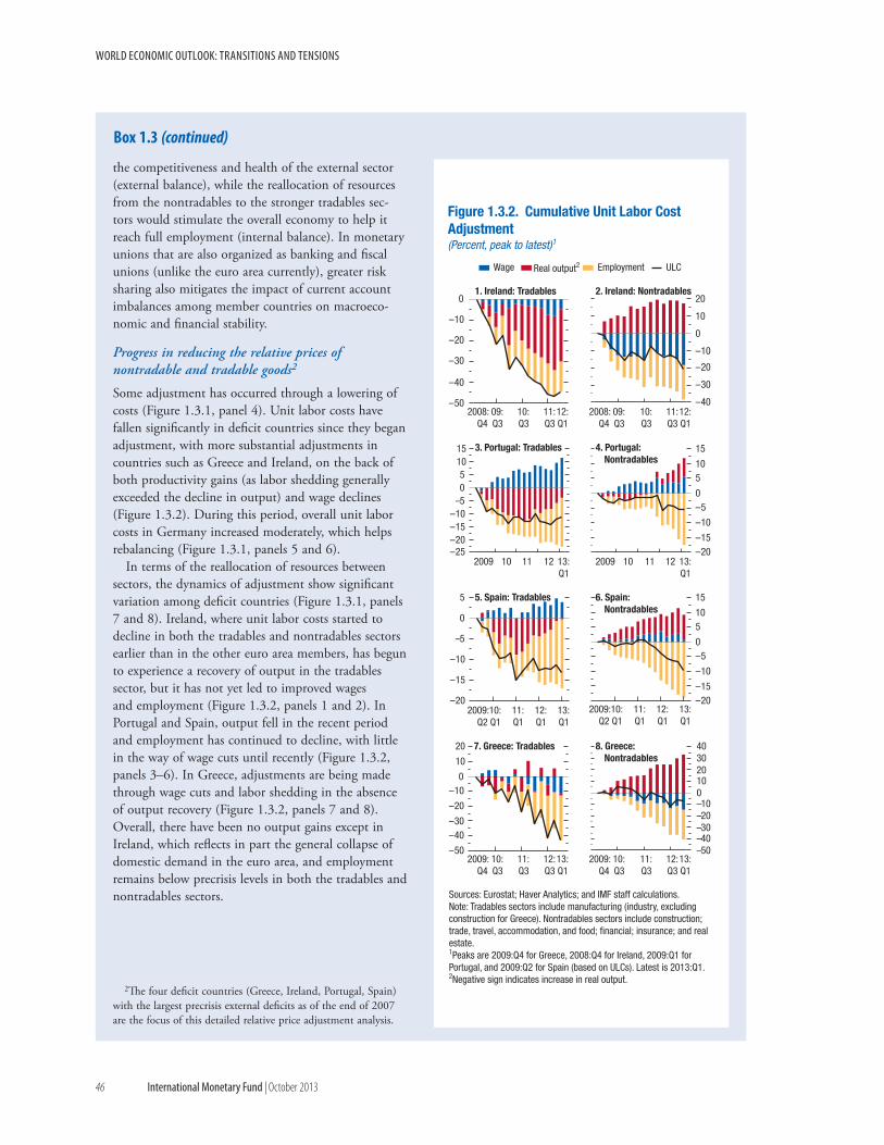
world economic outlook: transitions and tensions
46 international monetary Fund | October 2013
the competitiveness and health of the external sector (external balance), while the reallocation of resources from the nontradables to the stronger tradables sec-tors would stimulate the overall economy to help it reach full employment (internal balance). In monetary unions that are also organized as banking and fiscal unions (unlike the euro area currently), greater risk sharing also mitigates the impact of current account imbalances among member countries on macroeco-nomic and financial stability.
Progress in reducing the relative prices of nontradable and tradable goods2
Some adjustment has occurred through a lowering of costs (Figure 1.3.1, panel 4). Unit labor costs have fallen significantly in deficit countries since they began adjustment, with more substantial adjustments in countries such as Greece and Ireland, on the back of both productivity gains (as labor shedding generally exceeded the decline in output) and wage declines (Figure 1.3.2). During this period, overall unit labor costs in Germany increased moderately, which helps rebalancing (Figure 1.3.1, panels 5 and 6).
In terms of the reallocation of resources between sectors, the dynamics of adjustment show significant variation among deficit countries (Figure 1.3.1, panels 7 and 8). Ireland, where unit labor costs started to decline in both the tradables and nontradables sectors earlier than in the other euro area members, has begun to experience a recovery of output in the tradables sector, but it has not yet led to improved wages and employment (Figure 1.3.2, panels 1 and 2). In Portugal and Spain, output fell in the recent period and employment has continued to decline, with little in the way of wage cuts until recently (Figure 1.3.2, panels 3–6). In Greece, adjustments are being made through wage cuts and labor shedding in the absence of output recovery (Figure 1.3.2, panels 7 and 8). Overall, there have been no output gains except in Ireland, which reflects in part the general collapse of domestic demand in the euro area, and employment remains below precrisis levels in both the tradables and nontradables sectors.
2The four deficit countries (Greece, Ireland, Portugal, Spain) with the largest precrisis external deficits as of the end of 2007 are the focus of this detailed relative price adjustment analysis.
Box 1.3 (continued)
–50–40–30–20–10010203040
2009:Q4
10:Q3
11:Q3
12:Q3
13:Q1
–20–15
–10
–50
510
15
2009:Q2
10:Q1
11:Q1
12:Q1
13:Q1
–20–15
–10
–50
510
15
2009 10 11 12 13:Q1
–40
–30
–20
–10
0
10
20
2008:Q4
09:Q3
10:Q3
11:Q3
12:Q1
–50
–40
–30
–20
–10
0
2008:Q4
09:Q3
10:Q3
11:Q3
12:Q1
Figure 1.3.2. Cumulative Unit Labor Cost Adjustment(Percent, peak to latest)1
2. Ireland: Nontradables1. Ireland: Tradables
Wage Real output2 Employment ULC
–25–20–15–10
–505
1015
2009 10 11 12 13:Q1
3. Portugal: Tradables 4. Portugal:Nontradables
6. Spain:Nontradables
–20
–15
–10
–5
0
5
2009:Q2
10:Q1
11:Q1
12:Q1
13:Q1
8. Greece:Nontradables
–50
–40–30
–20
–100
10
20
2009:Q4
10:Q3
11:Q3
12:Q3
13:Q1
5. Spain: Tradables
7. Greece: Tradables
Sources: Eurostat; Haver Analytics; and IMF staff calculations.Note: Tradables sectors include manufacturing (industry, excluding construction for Greece). Nontradables sectors include construction; trade, travel, accommodation, and food; financial; insurance; and real estate.1Peaks are 2009:Q4 for Greece, 2008:Q4 for Ireland, 2009:Q1 for Portugal, and 2009:Q2 for Spain (based on ULCs). Latest is 2013:Q1.2Negative sign indicates increase in real output.
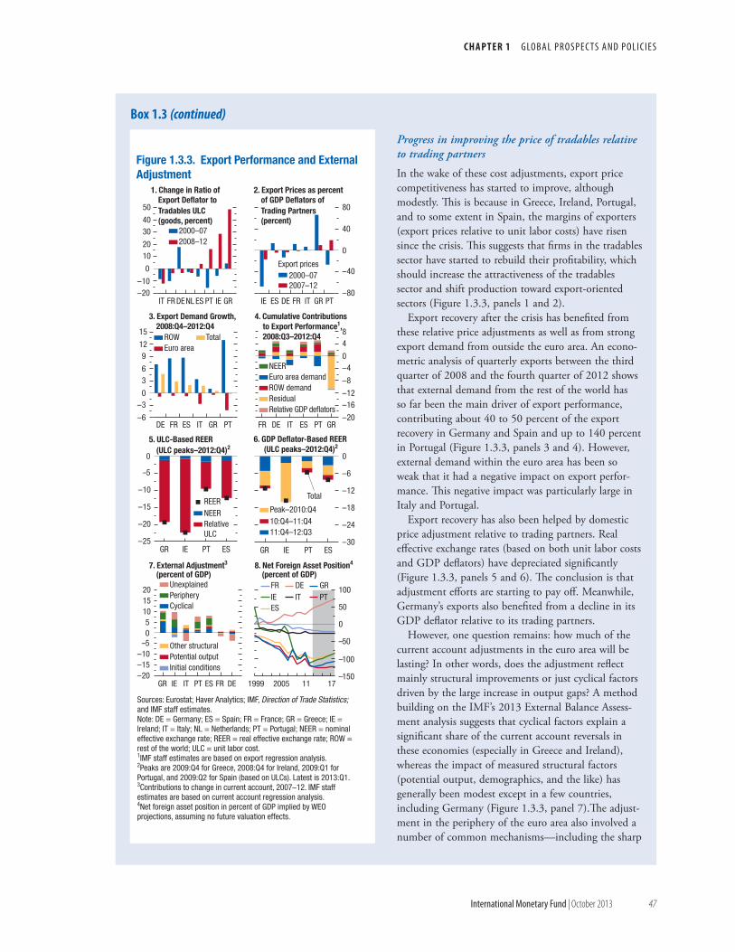
c h a p t e r 1 G lo b a l P r o s P e c ts a n d P o l i c i e s
international monetary Fund | October 2013 47
Progress in improving the price of tradables relative to trading partners
In the wake of these cost adjustments, export price competitiveness has started to improve, although modestly. This is because in Greece, Ireland, Portugal, and to some extent in Spain, the margins of exporters (export prices relative to unit labor costs) have risen since the crisis. This suggests that firms in the tradables sector have started to rebuild their profitability, which should increase the attractiveness of the tradables sector and shift production toward export-oriented sectors (Figure 1.3.3, panels 1 and 2).
Export recovery after the crisis has benefited from these relative price adjustments as well as from strong export demand from outside the euro area. An econo-metric analysis of quarterly exports between the third quarter of 2008 and the fourth quarter of 2012 shows that external demand from the rest of the world has so far been the main driver of export performance, contributing about 40 to 50 percent of the export recovery in Germany and Spain and up to 140 percent in Portugal (Figure 1.3.3, panels 3 and 4). However, external demand within the euro area has been so weak that it had a negative impact on export perfor-mance. This negative impact was particularly large in Italy and Portugal.
Export recovery has also been helped by domestic price adjustment relative to trading partners. Real effective exchange rates (based on both unit labor costs and GDP deflators) have depreciated significantly (Figure 1.3.3, panels 5 and 6). The conclusion is that adjustment efforts are starting to pay off. Meanwhile, Germany’s exports also benefited from a decline in its GDP deflator relative to its trading partners.
However, one question remains: how much of the current account adjustments in the euro area will be lasting? In other words, does the adjustment reflect mainly structural improvements or just cyclical factors driven by the large increase in output gaps? A method building on the IMF’s 2013 External Balance Assess-ment analysis suggests that cyclical factors explain a significant share of the current account reversals in these economies (especially in Greece and Ireland), whereas the impact of measured structural factors (potential output, demographics, and the like) has generally been modest except in a few countries, including Germany (Figure 1.3.3, panel 7).The adjust-ment in the periphery of the euro area also involved a number of common mechanisms—including the sharp
Box 1.3 (continued)
–25
–20
–15
–10
–5
0
GR IE PT ES
–150
–100
–50
0
50
100
1999 2005 11 17
–30
–24
–18
–12
–6
0
GR IE PT ES
–6
–30
36
912
15
DE FR ES IT GR PT
Figure 1.3.3. Export Performance and External Adjustment
4. Cumulative Contributions to Export Performance1, 2008:Q3–2012:Q4
6. GDP Deflator-Based REER (ULC peaks–2012:Q4)2
8. Net Foreign Asset Position4
(percent of GDP)
3. Export Demand Growth, 2008:Q4–2012:Q4
–20–15–10
–505
101520
GR IE IT PT ES FR DE
7. External Adjustment3
(percent of GDP)
–20
–16–12
–8
–40
48
FR DE IT ES PT GR
FR DE GRIE IT PTES
NEEREuro area demandROW demandResidualRelative GDP deflators
5. ULC-Based REER(ULC peaks–2012:Q4)2
REERNEERRelative ULC
Other structuralPotential outputInitial conditions
ROW TotalEuro area
UnexplainedPeripheryCyclical
Total
–20–10
0
1020
3040
50
IT FR DENL ES PT IE GR
2000–072008–12
–80
–40
0
40
80
IE ES DE FR IT GR PT
2. Export Prices as percentof GDP Deflators of Trading Partners(percent)
2000–072007–12
Export prices
1. Change in Ratio ofExport Deflator toTradables ULC(goods, percent)
Peak–2010:Q410:Q4–11:Q411:Q4–12:Q3
Sources: Eurostat; Haver Analytics; IMF, Direction of Trade Statistics; and IMF staff estimates.Note: DE = Germany; ES = Spain; FR = France; GR = Greece; IE = Ireland; IT = Italy; NL = Netherlands; PT = Portugal; NEER = nominal effective exchange rate; REER = real effective exchange rate; ROW = rest of the world; ULC = unit labor cost.1IMF staff estimates are based on export regression analysis.2Peaks are 2009:Q4 for Greece, 2008:Q4 for Ireland, 2009:Q1 for Portugal, and 2009:Q2 for Spain (based on ULCs). Latest is 2013:Q1.3Contributions to change in current account, 2007–12. IMF staff estimates are based on current account regression analysis.4Net foreign asset position in percent of GDP implied by WEO projections, assuming no future valuation effects.
world economic outlook: transitions and tensions
48 international monetary Fund | October 2013
reversal in capital flows following the crisis—that argu-ably reflect both structural and cyclical driving forces. The implication is that current account deficits could widen again significantly when cyclical conditions, including unemployment, improve, unless competi-tiveness improves further.
In the future, it will be very challenging to reduce external vulnerabilities by relying on net foreign assets to converge to more stable levels. Reducing net exter-nal liabilities to levels considered healthy elsewhere would likely require much larger relative price adjust-
ments than implied by the need to reverse past unit labor cost appreciation or to achieve current account surpluses. Under the baseline World Economic Outlook projections, without valuation effects, the net foreign asset positions of Greece, Ireland, Portugal, and Spain are expected to remain below minus 80 percent in 2018, implying that it will take a long time to undo the deterioraration of the net foreign asset position during 2000–12. Germany is expected to continue to accumulate external surpluses (Figure 1.3.3, panel 8).
Box 1.3 (continued)
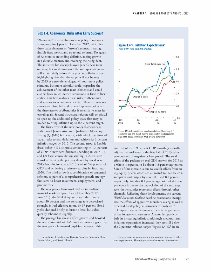
c h a p t e r 1 G lo b a l P r o s P e c ts a n d P o l i c i e s
international monetary Fund | October 2013 49
“Abenomics” is an ambitious new policy framework announced for Japan in December 2012, which has three main elements or “arrows”: monetary easing, flexible fiscal policy, and structural reforms. The goals of Abenomics are ending deflation, raising growth in a durable manner, and reversing the rising debt. The initiative has already buoyed Japan’s near-term outlook, but medium-term inflation expectations are still substantially below the 2 percent inflation target, highlighting risks that the target will not be met by 2015 as currently envisaged without more policy stimulus. But more stimulus could jeopardize the achievement of the other main elements and could also set back much-needed reductions in fiscal vulner-ability. This box analyzes these risks to Abenomics and reviews its achievements so far. There are two key takeaways. First, full and timely implementation of the three arrows of Abenomics is essential to meet its overall goals. Second, structural reforms will be critical to open up the additional policy space that may be needed to bring inflation up to the 2 percent target.
The first arrow of the new policy framework is is the new Quantitative and Qualitative Monetary Easing (QQME) framework, with which the Bank of Japan seeks to end deflation and achieve its 2 percent inflation target by 2015. The second arrow is flexible fiscal policy: (1) a stimulus amounting to 1.4 percent of GDP in new debt-financed spending in 2013–14; and (2) fiscal consolidation starting in 2014, with a goal of halving the primary deficit by fiscal year 2015 from its fiscal year 2010 level of 6.6 percent of GDP and achieving a primary surplus by fiscal year 2020. The third arrow is a combination of structural reforms, as part of a comprehensive growth strategy that aims to boost investment, employment, and productivity.
The new policy framework had an immediate financial market impact. From December 2012 to June 2013, the Nikkei equity price index rose by about 30 percent and the exchange rate depreciated strongly, in real effective terms, by 17 percent. Bond yields declined briefly to historic lows, but subse-quently rebounded slightly.
The package has already lifted growth and boosted the near-term outlook. IMF staff estimates suggest that the new policy framework explains between a third
and half of the 3.9 percent GDP growth (seasonally adjusted annual rate) in the first half of 2013, after two quarters of negative or low growth. The total effect of the package on real GDP growth for 2013 as a whole is expected to be about 1.3 percentage points. Some of this increase is due to wealth effects from ris-ing equity prices, which are estimated to increase con-sumption and output by about 0.3 and 0.2 percent, respectively. Another 0.4 percentage point of the out-put effect is due to the depreciation of the exchange rate; the remainder represents effects through other channels. Reflecting these developments, the current World Economic Outlook baseline projections incorpo-rate the effects of aggressive monetary easing as well as expected fiscal policy adjustments through 2015.
Despite these achievements, there is no guarantee of the longer-term success of Abenomics, particu-larly in increasing inflation. Although medium-term inflation expectations increased, they are still below the 2 percent inflation target (Figure 1.4.1).1 In an
1Survey-based measures show some modest increase in infla-tion expectations. The one-year-ahead measure increased to
Box 1.4. abenomics: risks after early Success?
The authors of this box are Dennis Botman, Benjamin Hunt, Zoltan Jakab, and René Lalonde.
Source: IMF staff calculations based on data from Bloomberg, L.P.1Estimated as a one-month moving average of implied consumer price index based on inflation swap bid and ask prices.
–0.5
0.0
0.5
1.0
1.5
2.0
Jan.2012
Jul.12
Jan.13
Jul. 13
Figure 1.4.1. Inflation Expectations1
(Year-over-year percent change)
Swap (8–10 years)
5-year break-even rate
Swap (3–5 years)
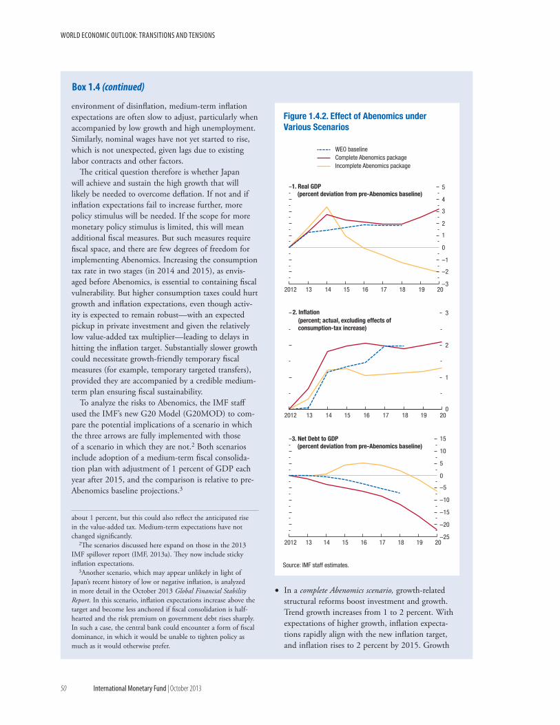
world economic outlook: transitions and tensions
50 international monetary Fund | October 2013
environment of disinflation, medium-term inflation expectations are often slow to adjust, particularly when accompanied by low growth and high unemployment. Similarly, nominal wages have not yet started to rise, which is not unexpected, given lags due to existing labor contracts and other factors.
The critical question therefore is whether Japan will achieve and sustain the high growth that will likely be needed to overcome deflation. If not and if inflation expectations fail to increase further, more policy stimulus will be needed. If the scope for more monetary policy stimulus is limited, this will mean additional fiscal measures. But such measures require fiscal space, and there are few degrees of freedom for implementing Abenomics. Increasing the consumption tax rate in two stages (in 2014 and 2015), as envis-aged before Abenomics, is essential to containing fiscal vulnerability. But higher consumption taxes could hurt growth and inflation expectations, even though activ-ity is expected to remain robust—with an expected pickup in private investment and given the relatively low value-added tax multiplier—leading to delays in hitting the inflation target. Substantially slower growth could necessitate growth-friendly temporary fiscal measures (for example, temporary targeted transfers), provided they are accompanied by a credible medium-term plan ensuring fiscal sustainability.
To analyze the risks to Abenomics, the IMF staff used the IMF’s new G20 Model (G20MOD) to com-pare the potential implications of a scenario in which the three arrows are fully implemented with those of a scenario in which they are not.2 Both scenarios include adoption of a medium-term fiscal consolida-tion plan with adjustment of 1 percent of GDP each year after 2015, and the comparison is relative to pre-Abenomics baseline projections.3
about 1 percent, but this could also reflect the anticipated rise in the value-added tax. Medium-term expectations have not changed significantly.
2The scenarios discussed here expand on those in the 2013 IMF spillover report (IMF, 2013a). They now include sticky inflation expectations.
3Another scenario, which may appear unlikely in light of Japan’s recent history of low or negative inflation, is analyzed in more detail in the October 2013 Global Financial Stability Report. In this scenario, inflation expectations increase above the target and become less anchored if fiscal consolidation is half-hearted and the risk premium on government debt rises sharply. In such a case, the central bank could encounter a form of fiscal dominance, in which it would be unable to tighten policy as much as it would otherwise prefer.
• In a complete Abenomics scenario, growth-related structural reforms boost investment and growth. Trend growth increases from 1 to 2 percent. With expectations of higher growth, inflation expecta-tions rapidly align with the new inflation target, and inflation rises to 2 percent by 2015. Growth
Box 1.4 (continued)
–25
–20
–15
–10
–5
0
5
10
15
2012 13 14 15 16 17 18 19 20
0
1
2
3
2012 13 14 15 16 17 18 19 20
–3
–2
–1
0
1
2
3
4
5
2012 13 14 15 16 17 18 19 20
Figure 1.4.2. Effect of Abenomics under Various Scenarios
Source: IMF staff estimates.
1. Real GDP(percent deviation from pre-Abenomics baseline)
2. Inflation(percent; actual, excluding effects ofconsumption-tax increase)
3. Net Debt to GDP(percent deviation from pre-Abenomics baseline)
WEO baselineComplete Abenomics packageIncomplete Abenomics package
c h a p t e r 1 G lo b a l P r o s P e c ts a n d P o l i c i e s
international monetary Fund | October 2013 51
reforms and fiscal consolidation are mutually reinforcing. Output is substantially higher than projected under the medium-term path before Abenomics, while the public-debt ratio starts to fall rather than increasing further.
• In an incomplete Abenomics scenario without growth-related structural reforms, investment and growth are lower. In addition, inflation expectations respond more sluggishly to economic conditions. In this environment, the authorities need to adopt additional fiscal stimulus to close the output gap and boost inflation in the near term. But this requires more fiscal adjustment later, partly because long-term interest rates rise by more, due to higher public financing requirements and higher risk premiums. The outcome is an eventual decline in the public-debt ratio to below the pre-Abenomics baseline. But output would remain below the pre-Abenomics baseline, and the 2 percent inflation target would be missed in the medium term. In the absence of more fiscal adjustment, debt would rise further, increasing the risk of a spike in bond yields and threatening financial stability.The simulations also suggest that negative spill-
over effects of Abenomics are likely to be mild. The depreciation in the exchange rate attributable to the QQME has a very small negative impact on short-term growth in the rest of the world. That said, the negative impacts are limited to a few countries (for example, China, Germany, Korea) and are on the order of 0.1 and 0.2 percentage point of GDP in the near term. Moreover, should the broader Abenomics package be successful, it would have clear positive net growth spillovers over the longer term if implemented completely. However, under an incomplete scenario these positive long-term benefits do not materialize.4
4See the 2013 IMF spillover report (IMF, 2013a) for more details.
In sum, the analysis highlights that the authorities need to be prepared to implement additional policy stimulus to bring inflation up to the 2 percent target. It also shows that this could increase the risks to Abe-nomics and that full and timely implementation of the three arrows will be essential to mitigate such risks.5 The analysis also underscores that the three arrows are closely connected. Structural reforms (for example, increasing the retirement age and the labor force par-ticipation of women and measures to raise productiv-ity growth) are needed for stronger long-term growth and fiscal sustainability.6 Fiscal sustainability is needed to gain fiscal space to help monetary policy bounded by the zero interest rate floor and to avoid a sharp increase in long-term real interest rates. Monetary policy easing is necessary to lower real interest rates to stimulate growth and help achieve the new inflation target, which will further enhance fiscal sustainabil-ity. The fact that fiscal consolidation may have to be delayed because of the need to maintain high growth for some time underscores the benefits of locking in longer-term fiscal gains through entitlement reform in the short term. Raising the retirement age and reforms to contain health care spending are obvious steps in this regard. Finally, the analysis suggests that in the short term, contingency plans for further unconven-tional monetary stimulus would be useful, given fiscal vulnerabilities.
5Ambitious structural reforms are also required to offset underlying deflation pressure from population aging.
6See IMF (2013e) for more details.
Box 1.4 (continued)
world economic outlook: transitions and tensions
52 international monetary Fund | October 2013
referencesAhn, Daniel P., 2012, Economic Consequences of Energy 2020,
Citi Energy 2020 Global Perspectives and Solutions Report.Ahuja, Ashvin, and Malhar Nabar, 2012, “Investment-Led
Growth in China: Global Spillovers,” IMF Working Paper No. 1267 (Washington: International Monetary Fund).
Ahuja, Ashvin, and Alla Myrvoda, 2012, “The Spillover Effects of a Downturn in China’s Real Estate Investment,” IMF Working Paper No. 12/266 (Washington: International Monetary Fund).
Arezki, Rabah, and Liugang Sheng, forthcoming, “How Do Giant Oil Discoveries Affect the Current Account?” IMF Working Paper (Washington: International Monetary Fund).
Baffes, John, and Allen Dennis, 2013, “Long Term Drivers of Food Prices,” World Bank Policy Research Working Paper No. 6455 (Washington: World Bank).
Beidas-Strom, Samya, and Andrea Pescatori, 2013, “Oil Price Volatility and the Role of Speculation” (unpublished; Wash-ington: International Monetary Fund).
Benes, Jaromir, Kevin Clinton, Roberto Garcia-Saltos, Marianne Johnson, Douglas Laxton, Peter Manchev, and Troy Mathe-son, 2010, “Estimating Potential Output with a Multivari-ate Filter,” IMF Working Paper No. 10/285 (Washington: International Monetary Fund).
Calvo, Guillermo A., Leonardo Leiderman, and Carmen M. Reinhart, 1996, “Inflows of Capital to Developing Countries in the 1990s,” The Journal of Economic Perspectives, Vol. 10, No. 2, pp. 123–39.
Carabenciov, Ioan, Charles Freedman, Roberto Garcia-Saltos, Douglas Laxton, Ondra Kamenik, and Petar Manchev, 2013, “GPM: The Global Projection Model with 6 Regions,” IMF Working Paper No. 13/87 (Washington: International Monetary Fund).
Decressin, Jörg, and Douglas Laxton, 2009, “Gauging Risks for Deflation,” IMF Staff Position Note No. 90/01 (Washington: International Monetary Fund).
Goodfriend, Marvin, 2003, “The Phases of U.S. Monetary Policy: 1987–2001,” Chapter 6 in Central Banking, Monetary Theory and Practice: Essays in Honor of Charles Goodhart, Vol. 1, ed. by Paul Mizen (Cheltenham, United Kingdom: Edward Elgar).
Hunt, Ben, and Dirk Muir, 2013, “Potential Implications of the United States Becoming Energy Self Sufficient” (unpublished).
International Monetary Fund (IMF), 2011, 2011 Spillover Report (Washington).
———, 2012a, 2012 Spillover Report (Washington).———, 2012b, “Investment-Led Growth in China: Global
Spillovers,” 2012 Spillover Report Background Papers.———, 2012c, People’s Republic of China: 2012 Article IV Con-
sultation, IMF Country Report No. 12/195 (Washington).———, 2012d, Russian Federation: 2012 Article IV Consultation,
IMF Country Report No. 12/217 (Washington).———, 2013a, 2013 Spillover Report (Washington).———, 2013b, Chile: Article IV Consultation Selected Issues,
IMF Country Report No. 13/198 (Washington).
———, 2013c, Colombia: Article IV Consultation Selected Issues, IMF Country Report No. 13/35 (Washington).
———, 2013d, Commodity Market Monthly, www.imf.org/commodities.
———, 2013e, Euro Area Policies: Selected Issues, IMF Country Report No. 13/232 (Washington).
———, 2013f, Japan: Article IV Consultation, IMF Country Report No. 13/253 (Washington).
———, 2013g, Nigeria: Article IV Consultation Selected Issues, IMF Country Report No. 13/116 (Washington).
———, 2013h, People’s Republic of China: Article IV Consulta-tion, IMF Country Report No. 13/211 (Washington).
———, 2013i, Qatar: Article IV Consultation Selected Issues, IMF Country Report No. 13/14 (Washington).
———, 2013j, Saudi Arabia: Selected Issues, IMF Country Report No. 13/230 (Washington).
———, 2013k, United States: Article IV Consultation, IMF Country Report No. 13/237 (Washington).
Kang, Joong Shik, Jay Shambaugh, Thierry Tressel, and Shengzu Wang, forthcoming, “Rebalancing and Growth in the Euro Area,” IMF Staff Discussion Note (Washington: International Monetary Fund).
Kumar, Manmohan S., 2003, Deflation: Determinants, Risks, and Policy Options, IMF Occasional Paper No. 221 (Washington: International Monetary Fund).
Laeven, Luc, and Fabian Valencia, 2012, “Systemic Banking Crises Database: An Update,” IMF Working Paper 12/63 (Washington: International Monetary Fund).
Loungani, Prakash, and Akito Matsumoto, forthcoming, Decoupling of Oil and Natural Gas Prices: Trial Separation or Permanent Split? IMF Working Paper (Washington: Interna-tional Monetary Fund).
Matheson, Troy D., 2011, “New Indicators for Tracing Growth in Real Time,” IMF Working Paper No. 11/43 (Washington: International Monetary Fund).
Okun, Arthur, 1962, “Potential GNP: Its Measurement and Sig-nificance,” Cowles Foundation Paper No. 190 (New Haven, Connecticut).
Phillips, A. W., 1958, “The Relation Between Unemployment and the Rate of Change of Money Wage Rates in the United Kingdom, 1861–1957,” Economica, Vol. 25, No. 100, pp. 283–99.
Roache, Shaun K., 2012, “China’s Impact on World Commod-ity Markets,” IMF Working Paper No. 12/115 (Washington: International Monetary Fund).
Sachs, Jeffrey D., Aaron Tornell, and Andres Velasco, 1996, “Financial Crises in Emerging Markets: The Lessons from 1995,” Brookings Papers on Economic Activity, Vol.1, pp. 147–215 (Washington: Brookings Institution).
U.S. Energy Information Administration (EIA), 2013, Techni-cally Recoverable Shale Oil and Shale Gas Resources: An Assessment of 137 Shale Formations in 41 Countries Outside the United States (Washington).