Global Positioning System (GPS) Basics: Using GPS …jontio.zapto.org/hda1/gps-basics-jonti.pdf · 2015-09-02 · is in an eﬀort to upgrade the features and performance of GPS

GPS Basics

Using GPS signals to find where you are

Jonathan Olds

[email protected]

http://jontio.zapto.org

c©Jonti 2015

http://jontio.zapto.org

Contents

1 GPS basics 1

1.1 GPS signal . . . . . . . . . . . . . . . . . . . . . . . . . . . . . . 1

1.2 What the GPS receiver does to the received WRX (t) signal . . . . 4

1.2.0.1 Obtaining the baseband signal R(t) . . . . . . . . 4

1.2.0.2 Stopping rotation . . . . . . . . . . . . . . . . . 5

1.2.0.3 C/A Code alignment . . . . . . . . . . . . . . . 5

1.3 Acquisition, tracking and NAV data extraction . . . . . . . . . . . 6

1.3.0.1 Extraction of NAV data using filtering . . . . . . 6

1.3.0.2 A metric for C/A code alignment and rotation . . 7

1.3.0.3 First-order linear approximations of unknown func-tions τ and Φ . . . . . . . . . . . . . . . . . . . 8

1.3.0.4 Further simplifications to the first-order linear ap-proximations of unknown functions τ and Φ inregard to acquisition . . . . . . . . . . . . . . . . 10

1.3.0.5 Acquisition . . . . . . . . . . . . . . . . . . . . . 11

1.3.0.6 Tracking . . . . . . . . . . . . . . . . . . . . . . 13

1.4 Observables . . . . . . . . . . . . . . . . . . . . . . . . . . . . . 14

1.4.1 The code observable . . . . . . . . . . . . . . . . . . . . . 15

i

CONTENTS

1.4.1.1 Calculating code based solutions . . . . . . . . . 16

1.4.1.2 Final code observable model . . . . . . . . . . . 19

1.4.2 The phase observable . . . . . . . . . . . . . . . . . . . . 20

1.4.2.1 Final phase observable model . . . . . . . . . . . 22

1.5 Selected proofs . . . . . . . . . . . . . . . . . . . . . . . . . . . . 25

1.5.1 Received phase using flight time approximation. . . . . . . 25

1.5.2 τ First-order linear approximation . . . . . . . . . . . . . . 25

1.5.3 Radial velocity with constant radial velocity offset ε . . . . 26

1.5.4 Maximum radial velocity and acceleration of the satellitewith respect to the receiver . . . . . . . . . . . . . . . . . 26

Nomenclature 29

Bibliography 31

ii

Chapter 1

GPS basics

Here we give a breif introduction to the basics of legacy GPS signals and how codebased position solutions can be obtained using them. This is the standard ob-servable that is used by consumers to obtain postion solutions. For compleatenesswe also mention the phase observable but do not attempt to describ how such anobservable can be used.

1.1 GPS signal

As of writing GPS is currently undergoing a modernization to improve both civilianand military use. Between 1990 and 2004 legacy satellites were launched whilefrom 2005 modernized satellites have been launched. According to the NationalCoordination Office for Space-Based Positioning, Navigation, and Timing [2] thisis in an effort to upgrade the features and performance of GPS. Currently GPStransmits on three different RF links from the satellites to end-users. The RFlinks are called L1, L2 and L5 and are named after the bands that they transmitin. Code Division Multiple Access (CDMA) is used as the channel access methodso all satellites used the same carrier frequencies. L1 has a nominal frequencyof 1575.42Mhz as seen from Earth, L2 1227.60Mhz and L5 1176.45Mhz. Thesenominal frequencies are modulated with various signals to aid navigation. Thecurrent GPS modernization consists of generally improving the hardware as wellas adding more signals that are sent over the RF links. The GPS modernizationcurrently underway will take many years and satellites producing signals such as

1

CHAPTER 1. GPS BASICS

L1C on L1 are not expected to be launched until 2016 with 24 satellites expectedby around 2026 [4]. We restrict our investigation here to that of legacy L1 signals.

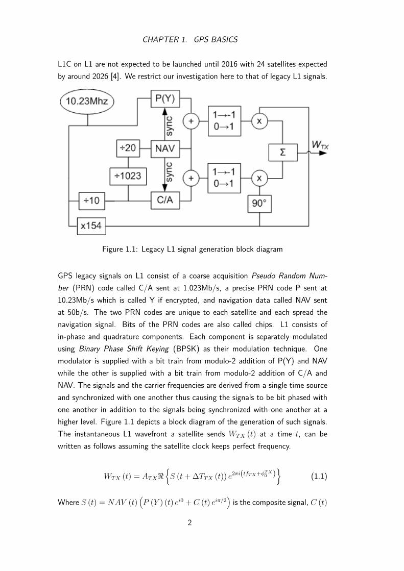
Figure 1.1: Legacy L1 signal generation block diagram

GPS legacy signals on L1 consist of a coarse acquisition Pseudo Random Num-ber (PRN) code called C/A sent at 1.023Mb/s, a precise PRN code P sent at10.23Mb/s which is called Y if encrypted, and navigation data called NAV sentat 50b/s. The two PRN codes are unique to each satellite and each spread thenavigation signal. Bits of the PRN codes are also called chips. L1 consists ofin-phase and quadrature components. Each component is separately modulatedusing Binary Phase Shift Keying (BPSK) as their modulation technique. Onemodulator is supplied with a bit train from modulo-2 addition of P(Y) and NAVwhile the other is supplied with a bit train from modulo-2 addition of C/A andNAV. The signals and the carrier frequencies are derived from a single time sourceand synchronized with one another thus causing the signals to be bit phased withone another in addition to the signals being synchronized with one another at ahigher level. Figure 1.1 depicts a block diagram of the generation of such signals.The instantaneous L1 wavefront a satellite sends WTX (t) at a time t, can bewritten as follows assuming the satellite clock keeps perfect frequency.

WTX (t) = ATX<{S (t+ ∆TTX (t)) e2πi(tfT X+φT X

0 )}

(1.1)

Where S (t) = NAV (t)(P (Y ) (t) ei0 + C (t) eiπ/2

)is the composite signal, C (t)

2


C/A code, P (Y ) (t) P(Y)-code, NAV (t) navigation data, φTX0 satellite oscillatorphase at time zero, ATX transmission amplitude, φTX0 satellite oscillator phase attime zero, fTX nominal satellite oscillator frequency as seen from Earth so as toaccount for general relativistic effects, f0 1575.42Mhz as seen from Earth, and τTX0

is the satellite composite signal offset at time zero. C,P (Y ) , NAV ∈ {−1, 1}and are functions so as to produce the correct composite signal where a mappingof 0 → 1 and 1 → −1 has been applied. At the receiver the instantaneous L1wavefront a receiver receives WRX (t) at a time t, can then be written as followsassuming no hindrance by the atmosphere.

WRX (t) = ARX<{S (t+ ∆TTX (t)−∆t (t)) e2πi((t−∆t(t))fT X+φT X

0 )}

(1.2)

Where ARX is reception amplitude and ∆t (t) is the transmission flight time fromthe satellite at transmission time to the receiver at reception time t. It’s importantto realize that ∆t (t) is not the flight time between the satellite and receiver attime t, but rather the flight time based as the receiver sees it. It is similar towhen a airplane passes by and one hears the sound of the plane lagging where theplane actually is. The flight time of the sound from the plane as determined bythe listener is different from the flight time one would get from calculating wherethe plane actually is to the user with respect to the same reception time.

3


1.2 What the GPS receiver does to the receivedWRX (t) signal

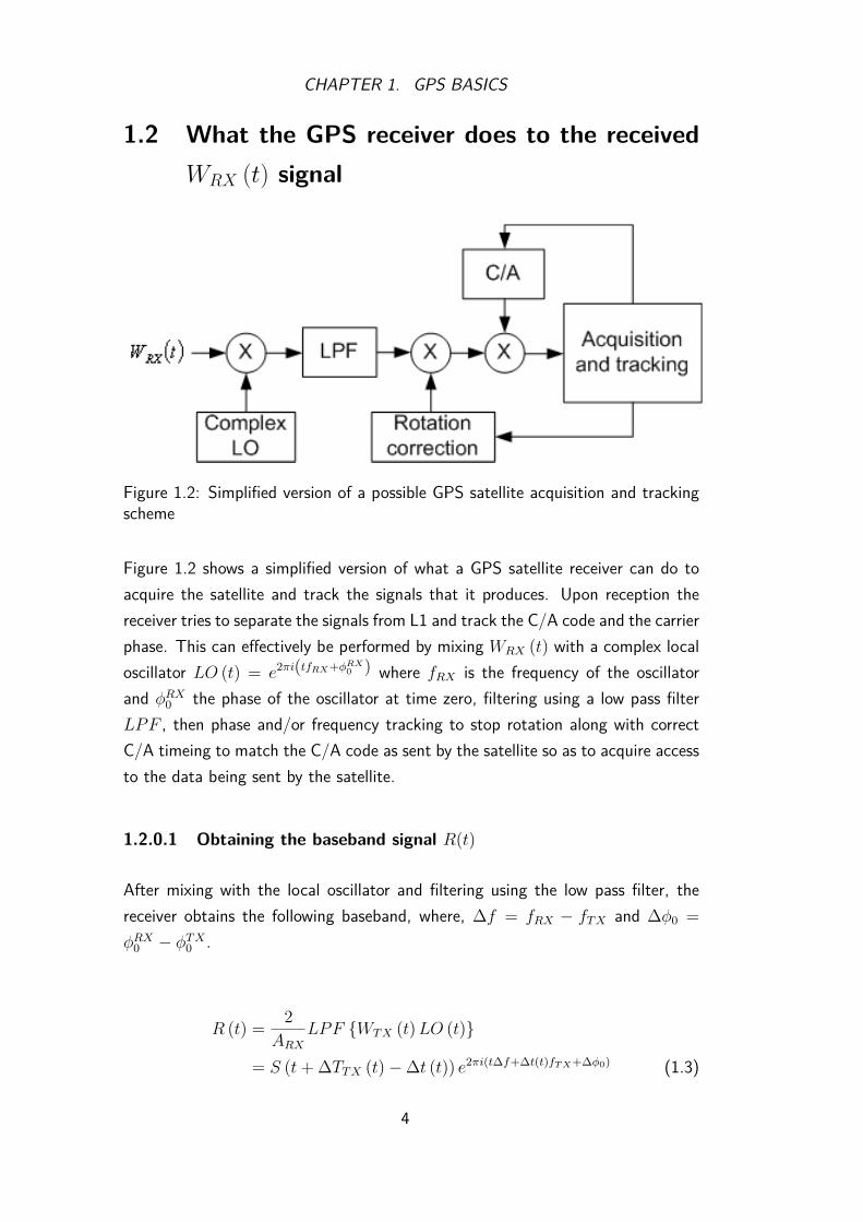
Figure 1.2: Simplified version of a possible GPS satellite acquisition and trackingscheme

Figure 1.2 shows a simplified version of what a GPS satellite receiver can do toacquire the satellite and track the signals that it produces. Upon reception thereceiver tries to separate the signals from L1 and track the C/A code and the carrierphase. This can effectively be performed by mixing WRX (t) with a complex localoscillator LO (t) = e2πi(tfRX+φRX

0 ) where fRX is the frequency of the oscillatorand φRX0 the phase of the oscillator at time zero, filtering using a low pass filterLPF , then phase and/or frequency tracking to stop rotation along with correctC/A timeing to match the C/A code as sent by the satellite so as to acquire accessto the data being sent by the satellite.

1.2.0.1 Obtaining the baseband signal R(t)

After mixing with the local oscillator and filtering using the low pass filter, thereceiver obtains the following baseband, where, ∆f = fRX − fTX and ∆φ0 =φRX0 − φTX0 .

R (t) = 2ARX

LPF {WTX (t)LO (t)}

= S (t+ ∆TTX (t)−∆t (t)) e2πi(t∆f+∆t(t)fT X+∆φ0) (1.3)

4


We define t∆f + ∆t (t) fTX + ∆φ0 as the received beat carrier phase (carrierphase).

1.2.0.2 Stopping rotation

We see that this is a constellation of four points that rotates due to the frequencydifference between the receiver’s local oscillator and the satellite’s oscillator, andalso rotates due to the radial motion of the satellite itself with respect to thereceiver.

If we let Φ (t) = t∆f + ∆t (t) fTX + ∆φ0 then we can correct for rotation bymultiplying R (t) as follows.

R (t) e−2πi(Φ(t)) = S (t+ ∆TTX (t)−∆t (t)) e2πi(Φ(t))e−2πi(Φ(t))

= S (t+ ∆TTX (t)−∆t (t)) (1.4)

This stops the constellation from rotating and removes any constant constellationrotation offset. This then resolves the composite signal. Hence we define Φ (t) asthe estimated received beat carrier phase by the receiver (estimated carrier phase).The constellation’s phase (or equivalently the constellation’s rotation offset) isdefined as the difference between the carrier phase and the estimated carrier phaset∆f +∆t (t) fTX + ∆φ0 − Φ (t). More generally as long as the estimated carrierphase is in phase with the carrier phase the constellation stops rotating and thereis no constant constellation rotation offset.

1.2.0.3 C/A Code alignment

After the constellation rotation has been stopped by letting the estimated carrierphase be in phase with the carrier phase, a local replica of the C/A code hasto be mixed with the composite signal and phase shifted in time until the localreplica of the C/A code is in phase with the one that is in the received compositesignal. We then define τ (t) as the C/A code alignment offset and is how muchthe incoming C/A is misaligned with the local replica. We define the local replica

5


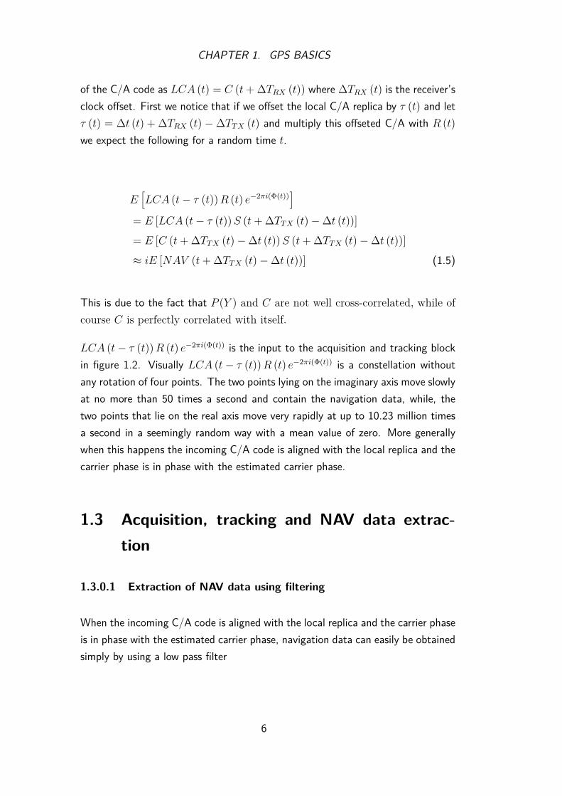
of the C/A code as LCA (t) = C (t+ ∆TRX (t)) where ∆TRX (t) is the receiver’sclock offset. First we notice that if we offset the local C/A replica by τ (t) and letτ (t) = ∆t (t) + ∆TRX (t) −∆TTX (t) and multiply this offseted C/A with R (t)we expect the following for a random time t.

E[LCA (t− τ (t))R (t) e−2πi(Φ(t))

]= E [LCA (t− τ (t))S (t+ ∆TTX (t)−∆t (t))]

= E [C (t+ ∆TTX (t)−∆t (t))S (t+ ∆TTX (t)−∆t (t))]

≈ iE [NAV (t+ ∆TTX (t)−∆t (t))] (1.5)

This is due to the fact that P (Y ) and C are not well cross-correlated, while ofcourse C is perfectly correlated with itself.

LCA (t− τ (t))R (t) e−2πi(Φ(t)) is the input to the acquisition and tracking blockin figure 1.2. Visually LCA (t− τ (t))R (t) e−2πi(Φ(t)) is a constellation withoutany rotation of four points. The two points lying on the imaginary axis move slowlyat no more than 50 times a second and contain the navigation data, while, thetwo points that lie on the real axis move very rapidly at up to 10.23 million timesa second in a seemingly random way with a mean value of zero. More generallywhen this happens the incoming C/A code is aligned with the local replica and thecarrier phase is in phase with the estimated carrier phase.

1.3 Acquisition, tracking and NAV data extrac-tion

1.3.0.1 Extraction of NAV data using filtering

When the incoming C/A code is aligned with the local replica and the carrier phaseis in phase with the estimated carrier phase, navigation data can easily be obtainedsimply by using a low pass filter

6


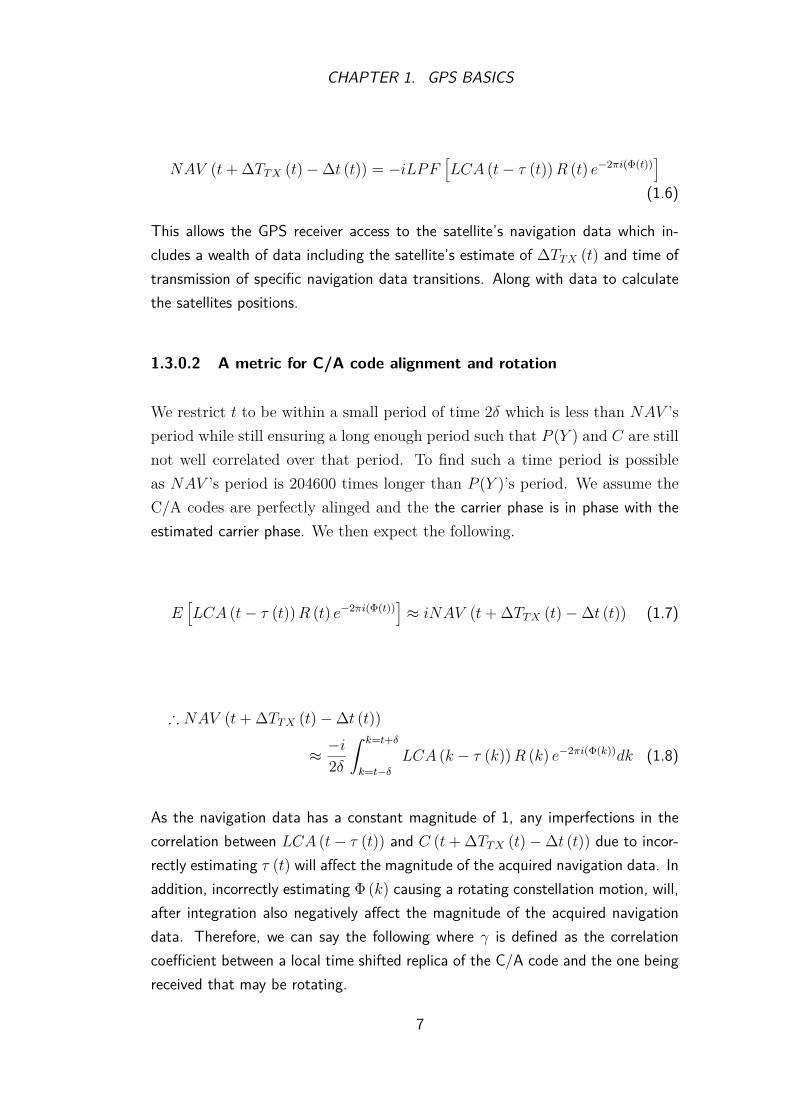
NAV (t+ ∆TTX (t)−∆t (t)) = −iLPF[LCA (t− τ (t))R (t) e−2πi(Φ(t))

](1.6)

This allows the GPS receiver access to the satellite’s navigation data which in-cludes a wealth of data including the satellite’s estimate of ∆TTX (t) and time oftransmission of specific navigation data transitions. Along with data to calculatethe satellites positions.

1.3.0.2 A metric for C/A code alignment and rotation

We restrict t to be within a small period of time 2δ which is less than NAV ’speriod while still ensuring a long enough period such that P (Y ) and C are stillnot well correlated over that period. To find such a time period is possibleas NAV ’s period is 204600 times longer than P (Y )’s period. We assume theC/A codes are perfectly alinged and the the carrier phase is in phase with theestimated carrier phase. We then expect the following.

E[LCA (t− τ (t))R (t) e−2πi(Φ(t))

]≈ iNAV (t+ ∆TTX (t)−∆t (t)) (1.7)

∴ NAV (t+ ∆TTX (t)−∆t (t))

≈ −i2δ

ˆ k=t+δ

k=t−δLCA (k − τ (k))R (k) e−2πi(Φ(k))dk (1.8)

As the navigation data has a constant magnitude of 1, any imperfections in thecorrelation between LCA (t− τ (t)) and C (t+ ∆TTX (t)−∆t (t)) due to incor-rectly estimating τ (t) will affect the magnitude of the acquired navigation data. Inaddition, incorrectly estimating Φ (k) causing a rotating constellation motion, will,after integration also negatively affect the magnitude of the acquired navigationdata. Therefore, we can say the following where γ is defined as the correlationcoefficient between a local time shifted replica of the C/A code and the one beingreceived that may be rotating.

7


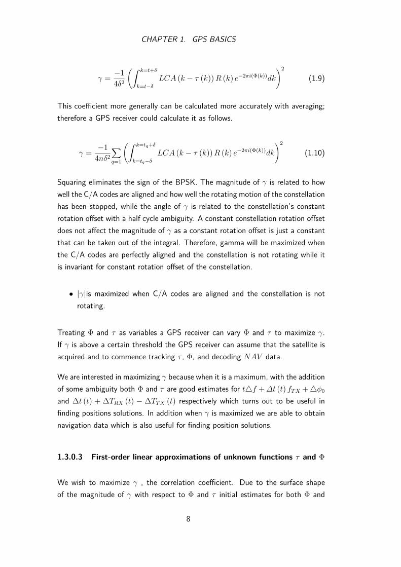
γ = −14δ2

(ˆ k=t+δ

k=t−δLCA (k − τ (k))R (k) e−2πi(Φ(k))dk

)2

(1.9)

This coefficient more generally can be calculated more accurately with averaging;therefore a GPS receiver could calculate it as follows.

γ = −14nδ2

∑q=1

(ˆ k=tq+δ

k=tq−δLCA (k − τ (k))R (k) e−2πi(Φ(k))dk

)2

(1.10)

Squaring eliminates the sign of the BPSK. The magnitude of γ is related to howwell the C/A codes are aligned and how well the rotating motion of the constellationhas been stopped, while the angle of γ is related to the constellation’s constantrotation offset with a half cycle ambiguity. A constant constellation rotation offsetdoes not affect the magnitude of γ as a constant rotation offset is just a constantthat can be taken out of the integral. Therefore, gamma will be maximized whenthe C/A codes are perfectly aligned and the constellation is not rotating while itis invariant for constant rotation offset of the constellation.

• |γ|is maximized when C/A codes are aligned and the constellation is notrotating.

Treating Φ and τ as variables a GPS receiver can vary Φ and τ to maximize γ.If γ is above a certain threshold the GPS receiver can assume that the satellite isacquired and to commence tracking τ , Φ, and decoding NAV data.

We are interested in maximizing γ because when it is a maximum, with the additionof some ambiguity both Φ and τ are good estimates for t4f +∆t (t) fTX +4φ0

and ∆t (t) + ∆TRX (t) − ∆TTX (t) respectively which turns out to be useful infinding positions solutions. In addition when γ is maximized we are able to obtainnavigation data which is also useful for finding position solutions.

1.3.0.3 First-order linear approximations of unknown functions τ and Φ

We wish to maximize γ , the correlation coefficient. Due to the surface shapeof the magnitude of γ with respect to Φ and τ initial estimates for both Φ and

8


τ are required. Without good initial estimates, γ is dominated by noise makingstandard tracking schemes such as Phase Locked Loop (PLL), Frequency LockedLoop (FLL), Delay Locked Loop (DLL) and early/late time useless. It’s like tryingto track an ant crawling in long grass; you have to find it first before you can trackit as the grass makes it difficult to see the ant from afar.

First we create a first order linear approximation model of how Φ and τ change.We have already seen that when Φ (t) = t4f + ∆t (t) fTX +4φ0 and τ (t) =∆t (t)+∆TRX (t)−∆TTX (t) we are able to stop rotation and align our local C/Acode replica with the incoming one. Therefore, these are the Φ and τ that we arelooking for. Linear approximations of these two equations are written below whereF (tm) = (∆f + ∆fTX (tm)), ∆fTX (tm) is the change of frequency of fTX dueto Doppler at time tm, where a positive value is for the satellite moving away fromthe receiver and θ (tm) and Ξ (tm) are some constants. Proofs can be found in1.5.1 and 1.5.2.

Φ (t) ≈ tF (tm) + θ (tm) (1.11)

τ (t) ≈ (t− tm)F (tm) −1f0

+ Ξ (tm) (1.12)

These approximations are only valid if F (tm) does not change to rapidly aroundtime tm. The maximum rate at which velocity will change is about 0.1178ms−2

and is when the satellite is directly overhead (1.5.4). On the L1 band this impliesthat the constellation rotation speed will change by less than about 0.9Hzs−1 ifF (tm) is left unchanged in equation 1.13 ( see 1.5.3 and 1.5.4). Now comparethis to the range of F (tm). ∆fTX (tm) can be as large as about ±5 kHz (1.5.4),and depending on the receiver clock accuracy∆f could be out by another 5 kHz ifwe assume a receiver clock accuracy of 3.5 ppm. This means the range of F (tm)is in the order of 20 kHz. If we restrict our time of interest to 1ms, then, F (tm)will change by less than 0.0009Hz which is far less than the range of the 20 kHzof F (tm). Therefore, for short periods of time this is a valid approximation.

Equations 1.11 and 1.12 form an approximate model of how Φ and τ will changein the short term.

9


1.3.0.4 Further simplifications to the first-order linear approximations ofunknown functions τ and Φ in regard to acquisition

In figure 1.2 the input of the acquisition and tracking block as we have alreadyseen is written as in equation 1.13.

LCA (t− τ (t))R (t) e−2πi(Φ(t)) (1.13)

To acquire Φ and τ initially we can make further simplifications to equations 1.11and 1.12. θ (tm) in equation 1.11 when placed in equation 1.13 has no effecton changing constellation rotation with respect to time. 1.13 will still be a non-rotating four-point constellation but just with a constant rotation offset of θ (tm)cycles. As we have already mentioned in equation 1.10, any constant rotationoffset has no effect on the magnitude of the correlation coefficient. Therefore wecan ignore θ (tm) when initially acquiring Φ.

The carrier wave frequency is 1540 times greater than the bit rate of the C/Acode. As frequency times time is phase, if F = 10, 000Hz then it takes 0.025msfor Φ to change by a quarter of the cycle, while it takes 38.5ms for the C/Acode to change by a quarter of a chip. If we then assume a digitalization of R atthe rate of 4.092Mb/s and sampling 1ms worth of R, more often than not wecouldn’t even detect the difference between F = 0 and F = 10, 000 in the C/Acode directly while it would be easy to detect in the carrier wave.

Due to these two points we make the following two approximations when consid-ering initial acquisition of Φ and τ . Here we acknowledge that the constellationwill have an arbitrary constant rotation offset, are only valid for periods of time ofa few milliseconds, and baseband sampling rate is no more than a few times perchip.

Φ (t) ≈ tF (tm) (1.14)

τ (t) ≈ Ξ (tm) (1.15)

10


1.3.0.5 Acquisition

With these two approximations 1.14 and 1.15 the receiver can do a two-dimensionalsearch, F with a frequency dimension and the other Ξ with a time dimension to findthe point that maximizes the correlation coefficient in equation 1.10. Assuminga receiver clock accuracy of 3.5 ppm, the receiver would have to search from−10 kHz to 10 kHz. As the C/A code is a periodic function with a period of 1ms, the receiver would have to search from 0 ms to 1 ms.

Estimating F and Ξ by trying to maximize the correlation between the local C/Acode replica with the incoming one turns out to be computationally demanding us-ing more energy than tracking, and is a major concern for GPS receivers. Becauseof this much research has been directed towards this problem to reduce the com-putational effort to estimate these two parameters [7]. A parallelized 2D searchby using Fast Fourier Transform (FFT) is a conventional method currently used insoftware defined receivers [7].

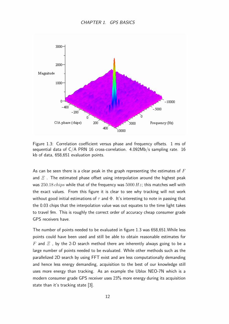
As an example we cross-correlated a local C/A code replica with an incomingone on L1. We used a sample rate of 4.092Mb/s being four times the nominalfrequency of the chip rate and searched by varying the frequency term by ±10 kHzin steps of 125Hz and then using cross correlation varying the time term by nomore than ±511.5 chips (±511.5 chips covers the entire 1ms). Navigation datawas simulated by using random data, while no P(Y) data was added. An offsetof 5000Hz was applied to the 1.57542GHz carrier frequency and a phase offsetof 250.15 chips was applied to the C/A code of the incoming signal. Using 1msworth of sequential incoming data, figure 1.3 was obtained.

11


Figure 1.3: Correlation coefficient versus phase and frequency offsets. 1 ms ofsequential data of C/A PRN 16 cross-correlation. 4.092Mb/s sampling rate. 16kb of data, 658,651 evaluation points.

As can be seen there is a clear peak in the graph representing the estimates of Fand Ξ . The estimated phase offset using interpolation around the highest peakwas 250.18 chips while that of the frequency was 5000Hz; this matches well withthe exact values. From this figure it is clear to see why tracking will not workwithout good initial estimations of τ and Φ. It’s interesting to note in passing thatthe 0.03 chips that the interpolation value was out equates to the time light takesto travel 9m. This is roughly the correct order of accuracy cheap consumer gradeGPS receivers have.

The number of points needed to be evaluated in figure 1.3 was 658,651.While lesspoints could have been used and still be able to obtain reasonable estimates forF and Ξ , by the 2-D search method there are inherently always going to be alarge number of points needed to be evaluated. While other methods such as theparallelized 2D search by using FFT exist and are less computationally demandingand hence less energy demanding, acquisition to the best of our knowledge stilluses more energy than tracking. As an example the Ublox NEO-7N which is amodern consumer grade GPS receiver uses 23% more energy during its acquisitionstate than it’s tracking state [3].

12


1.3.0.6 Tracking

Once the acquisition has been performed and the point of the maximum correlationcoefficient has been found, the receiver can then track τ and Φ using standardtechniques such as PLL, FLL, DLL and early/late tracking methods. The linearapproximations do not stop the maximum correlation coefficient point from movingbut it slows it down sufficiently that one can treat it as a stationary point until ithas been found then one can simply track it as it moves.

From acquisition, estimates for F and Ξ are obtained, which via equation 1.12gives an estimate for τ (t). To track τ (t) then early/late tracking can be used.Such a method usually consists of three locally produced C/A replicas, one slightlyahead of what is expected from the satellite, one as expected from the satellite,and one slightly behind what is expected from the satellite.

Early LCA (t− τ (t) + ξ)

Prompt LCA (t− τ (t))

Late LCA (t− τ (t)− ξ)

These three C/A replicas are then each correlated with R (t) e−2πi(Φ(t)) to producethree correlation coefficients (γE ,γP , γL) and using interpolation a new estimatefor τ (t) can be obtained to keep the code aligned. Keeping the code aligned isthe one of the two requirements for maximizing γ.

LCA (t− τ (t))R (t) has the effect of removing the C/A code from R. This re-moval is called wiping the code. Once it is removed a carrier tracking schemesuch as a PLL can be used on LCA (t− τ (t))R (t) because in one directionit appears as a standard BPSK signal. A costas PLL could be performed onLCA (t− τ (t))R (t) to estimate Φ (t) as it is invariant to the navigation transi-tions. Assume that we designed the costas loop to align on the imaginary axis.Then, the costas loop will align NAV ’s BPSK signal along the imaginary axis withan ambiguity as to which way around it is aligned. The costas loop will also stopthe constellation from rotating which is one of the two requirements for maximizingγ.

13


So, using code tracking and carrier tracking simultaneously the maximum point ofcorrelation can be continuously tracked. It is not sufficient for a receiver solely totrack only one of τ (t) or Φ (t); both need to be tracked simultaneously.

We have already seen that in 1.3.0.2 τ (t) = ∆t (t)+∆TRX (t)−∆TTX (t) impliesmaximum correlation. Due to the 1ms C/A ambiguity the converse is not true.Therefore we can say that maximum correlation implies τ (t) = ∆t (t)+∆TRX (t)−∆TTX (t) +M/1000 where M is some fixed integer.

Likewise Φ (t) = t4f + ∆t (t) fTX +4φ0 implies maximum correlation but dueto carrier phase cycle ambiguity and that gamma is maximized for any constantrotation offset the converse is not true. The costas loop removes the constantrotation offset with an ambiguity of half a cycle, and if the PLL accumulates itsphase offset rather than resetting it as it passes through an angle of zero, thenmaximum correlation implies Φ (t) = t4f + ∆t (t) fTX +4φ0 + N/2 for somefixed integer N .

τ and Φ when these ambiguities are considered become the two observables used byalmost all low end consumer grade GPS receivers for position solution calculations.

1.4 Observables

Observables are measurements taken by the GPS receiver of quantities that theGPS receiver can directly measure. Observables do not directly tell you wherethe GPS receiver is situated but with using various techniques will allow you tocalculate position solutions that do tell you where the GPS is situated. The twoobservables we consider are the code observable and the phase observable.

We have seen by tracking the maximum point of γ using early late timing and acostas PLL that we have found τ (t) = ∆t (t)+∆TRX (t)−∆TTX (t)+M/1000 forsome fixed integer M and Φ (t) = t4f +∆t (t) fTX +4φ0 +N/2 for some fixedinteger N . These are the code observable and the phase observable respectivelyso far. However, there are some added complications and the form they take candiffer.

14


1.4.1 The code observable

Once γ is tracked the receiver has access to the navigation data. The navigationdata is sent as 30 bits per word. There are 10 words in a subframe taking 6seconds to transmit. Each subframe contains a Hand Over Word (HOW) wordthat indicates the exact time when the leading-edge of the first bit of the navigationdata was transmitted from the satellite. In the satellite the first bit of every NAVdata transition is aligned to first chip of the the C/A code. This is possible as theyare derived from the same oscillator (see 1.1). Figure 1.4 shows the C/A NAVtiming relationship.

Figure 1.4: C/A NAV timing relationship

Because of this unique time stamp every 6 seconds and that the receiver is con-tinuously tracking the C/A code of the satellite, each chip of a C/A code can beuniquely identified with an exact time of transmission. Therefore, the receiver canresolve the ambiguity M in the code observable and hence can estimate τ (t) suchthat τ (t) = ∆t (t) + ∆TRX (t)−∆TTX (t).

Usually the code observable is in units of meters and is called the pseudorange.Converting τ (t) into meters by multiplying by the speed of light c results in thefollowing pseudorange equation where the variable time has been removed for

15


brevity and ρ is the range from the transmitter at transmission time to receive atreception time.

p = ρ+ c (∆TRX −∆TTX) (1.16)

1.4.1.1 Calculating code based solutions

The satellite’s current clock bias∆TTX is transmitted in the navigation data andtherefore is a known value. The unknown values are therefore the receiver’s po-sition and clock bias; together these are P = [x, y, z,∆TRX ]. This means thepseudorange is a function of these unknown variables. Obtaining one such pseu-doranges for a satellite results in the following nonlinear equation.

pn (P) = ρn + c (∆TRX −∆T nTX) (1.17)

Because of the ease of solving linear equations, linearization of this equation usinga first order Taylor expansion is sensible for deriving a generalized method ofsolving sets of pseudoranges of arbitrary sizes. We let an estimated solution beP =

[x, y, z,∆TRX

]for time of reception. Then, a first order Taylor expansion

for pn around P is as follows.

pn (P) ≈ pn(P)

+ (x− x) ∂

∂xpn

∣∣∣∣∣P

+ (y − y) ∂

∂ypn

∣∣∣∣∣P

+ (z − z) ∂

∂zpn

∣∣∣∣∣P

+(∆TRX − ˆ∆TRX

) ∂

∂∆TRXpn

∣∣∣∣∣P

(1.18)

Given a satellite’s position Sn = [xn, yn, zn] at time of transmission for a pseu-dorange pn, then, the partial derivatives can be calculated given ρn (x, y, z) =√

(x− xn)2 + (y − yn)2 + (z − zn)2. Therefore, upon evaluation, equation 1.18can be written as follows.

16


pn (P)− pn(P)≈ (x− x) (x− xn)

ρn

+ (y − y) (y − yn)ρn

+ (z − z) (z − zn)ρn

+(∆TRX − ˆ∆TRX

)c (1.19)

Given a good estimate P, this equation has four independent unknowns, henceat least four equation just like it are needed to solve the unknowns. These fourequations require the receiver’s clock bias to be the same for all equations andthe receiver’s position to be the same for all equations. Therefore, the receiverhas to obtain four pseudoranges simultaneously. A set of m such pseudoranges fordifferent satellites obtained simultaneously are given below.

p1 (P) = ρ1 + c(∆TRX −∆T 1

TX

)...

pm (P) = ρm + c (∆TRX −∆TmTX) (1.20)

Because equation 1.19 is linear this set of pseudo ranges can be written in matrixform as follows.

(x−x1)ρ1

(y−y1)ρ1

(z−z1)ρ1

c... ... ... ...

(x−xm)ρm

(y−ym)ρm

(z−zm)ρm

c

(x− x)(y − y)(z − z)(

∆TRX − ˆ∆TRX)

≈p1 (P)− p1

(P)

...pm (P)− pm

(P)

(1.21)

Using bold type notation vectors or matrices, this has the form of A(P− P

)≈ b

where A, b, and P are known. Using LS and rearranging for the unknown yieldsP ≈

(ATA

)−1ATb + P. The right-hand side of this equation when calculated

yields only an approximation of the desired solution P. Therefore(ATA

)−1ATb+

P is another solution estimate and we denote it as Pn =[xn, yn, zn,∆TRXn

]. So

17


we have seen a way of obtaining a new solution estimate from an old solutionestimate. This process can be reiterated as the following algorithm describes.

Algorithm 1.1 Iterative LS solution using code observable

1. P0 = [0, 0, 0, 0] , n = 0

2. increment n

3. estimate reception time trx = TRX − ˆ∆TRX

4. calculate Sm at time trx

5. calculate Sm at time trx − ‖Sm − [xn, yn, zn]‖ /c and reitterate a few times

6. if ��∃(ATA

)−1stop wih error

7. Pn =(ATA

)−1ATb + Pn−1

8. if ( ‖[xn, yn, zn]− [xn−1, yn−1, zn−1]‖ < less than desired error) stop

9. if (n > to big ) stop with error

10. goto 2

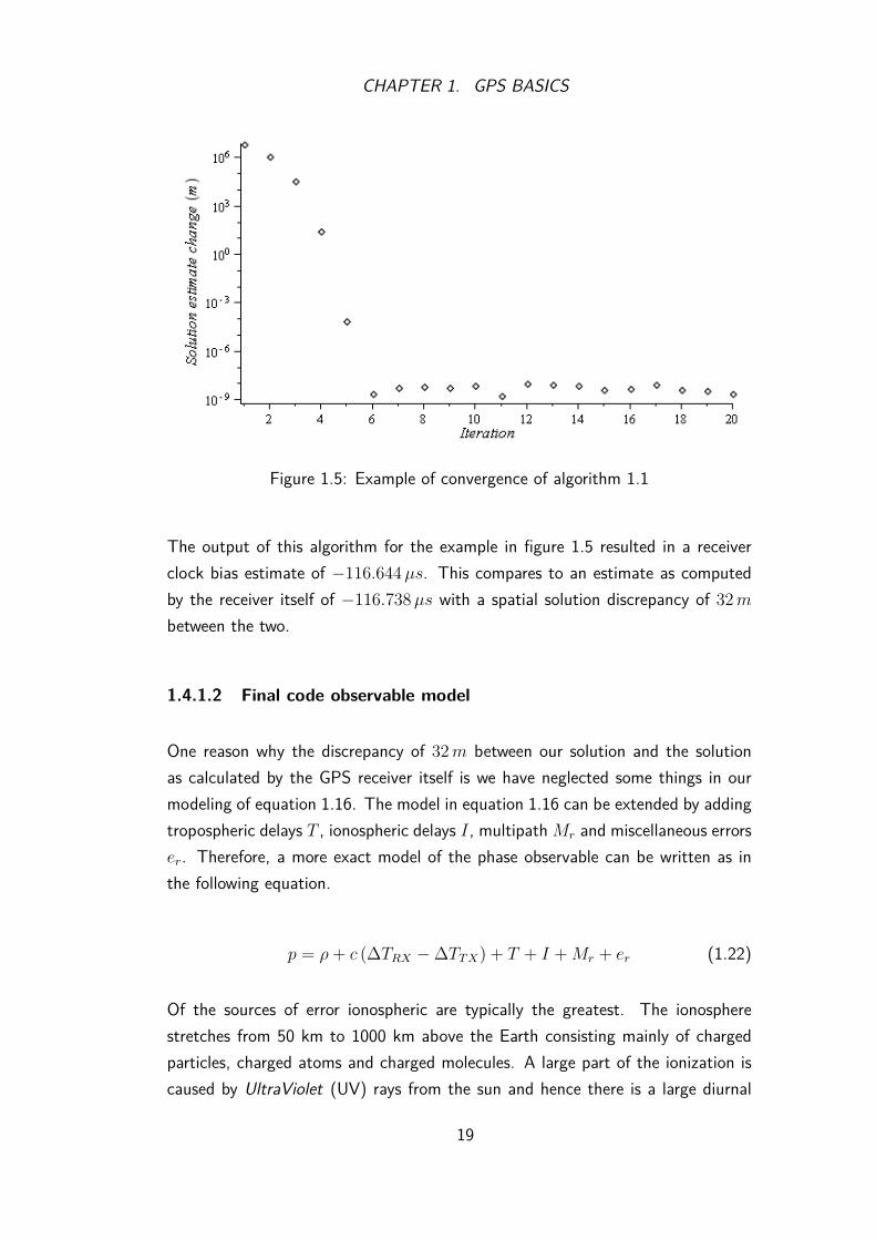
The correction made to the time of reception as believed by the receiver TRX toproduce an estimate of the reception time in step 3, for most receivers would besmall in the order of less than a millisecond and could be conceivably ignored.The correction needed for calculating an estimate of the time of transmission asperformed in step 5 is generally comparatively large, and is in the order of around60ms being the approximate flight time from the satellite to the receiver; this stepcan’t be ignored.

Figure 1.5 shows an example of algorithm 1.1 converging for a set of six satellitesand code observations taken of them. As can be seen using the center of the Earthas the initial estimate within six iterations the algorithm has converged.

18


Figure 1.5: Example of convergence of algorithm 1.1

The output of this algorithm for the example in figure 1.5 resulted in a receiverclock bias estimate of −116.644µs. This compares to an estimate as computedby the receiver itself of −116.738µs with a spatial solution discrepancy of 32mbetween the two.

1.4.1.2 Final code observable model

One reason why the discrepancy of 32m between our solution and the solutionas calculated by the GPS receiver itself is we have neglected some things in ourmodeling of equation 1.16. The model in equation 1.16 can be extended by addingtropospheric delays T , ionospheric delays I, multipathMr and miscellaneous errorser. Therefore, a more exact model of the phase observable can be written as inthe following equation.

p = ρ+ c (∆TRX −∆TTX) + T + I +Mr + er (1.22)

Of the sources of error ionospheric are typically the greatest. The ionospherestretches from 50 km to 1000 km above the Earth consisting mainly of chargedparticles, charged atoms and charged molecules. A large part of the ionization iscaused by UltraViolet (UV) rays from the sun and hence there is a large diurnal

19


change in the Total Electron Count (TEC) which in turn effects the ionosphericcorrection term I. The ionosphere can produce a satellite range error as little as1 m to as much as 100 m [1]. The ionospheric correction term is frequency de-pendent and with dual band receivers ionospheric free combinations of observablesare possible. For singleband receivers no such combination is possible, insteadKlobuchar ionospheric model is used for singleband receivers GPS. Klobuchar co-efficients are transmitted in the navigation message so that the receiver can thenestimate ionospheric correction terms. The Klobuchar algorithm corrects about50% of the ionospheric errors [5].

The important thing for us in this section is that we are able to obtain an approxi-mate solution, the spatial component with some sort of accuracy less than 100m,and a time accuracy of some sort less than a 1µs. This is all we are concernedabout regarding the code observable.

1.4.2 The phase observable

The phase observable is a measured quantity taken by the GPS receiver for a par-ticular satellite for a particular time. Phase observables allows higher accuracy GPSmeasurements to be made than compared to that of ones solely using code observ-ables. This is due to the much shorter wavelength of GPS carrier than compared tothe chip length of the code observable. The wavelength of L1 is approximately 20cm compared to approximately 300 m length for the code chip of the C/A signaland can result in a correspondingly large increase in accuracy. The measurementcomes from monitoring the phase difference between the received satellite carrierand a reference oscillator on the GPS receiver. The receiver accumulates this in-stantaneous phase difference by tracking and outputs this to the user as the phaseobservable. Figure 1.6 shows a block diagram of what the GPS receiver is doingwhen observing a satellite for the phase observable neglecting all signals sent onthe carrier such as C/A, navigation and P(Y) code.

20


Figure 1.6: Simplified block diagram of phase measurement

For GPS, phase is customary in units of cycles rather than radians or degrees forGPS work. Phase is the argument inside a trigonometric function that acceptsunits of cycles. ΦS is the phase of the carrier of the satellite while ΦU is thereceiver’s reference phase. Both ΦS and ΦU can become arbitrarily large.

Inherent in accumulation of phase is an ambiguity N that depends on when youstarted accumulating phase. In addition to the ambiguity there is the possibility ofmissing some rotations. Counting the number of times a car tire rotates dependson when you started counting its rotations and also depends on whether you missedany rotations. While GPS receivers try to continuously track the phase, this is notalways possible. Due to noise, loss of signal or turning the GPS receiver off andon again, the tracking of the phase can be lost resulting in an integer change inthe value of N . This produces what is called a “cycle slip”. So, ideally this phaseambiguity should be fixed while the satellite is being tracked but due to cycle slipsoccasionally it will change.

As we have seen satellites don’t send out continuous waves, they are modulatedwith two BPSK signals, one in the quadrature phase and the other in the in-phase.Code tracking has the effect of wiping the C/A code from one of the BPSK signalsbut still leaves the navigation adding a level of complexity when trying to trackit. When the BPSK data is not used to regenerate the original carrier wave ahalf cycle ambiguity in the carrier phase is introduced into the phase observable

21


and it is said that the phase observable has a code factor of two Cf = 2. Whenthe BPSK data is used to regenerate the original carrier wave, the original carrierwave can be fully regenerated with an ambiguity of one cycle and it is said thatthe phase observable has a code factor of two Cf = 1. Thus the ambiguity of thephase observable can be reduced when a code factor of one is used.

1.4.2.1 Final phase observable model

As we have seen tracking the carrier phase maximizes γ which in turn means theaccumulated phase while tracking is Φ = t4f + ∆tfTX +4φ0 + N/2 for somefixed integer N when using a costas PLL. When considering the code factor thiscan be written as follows.

Φ = t4f +∆tfTX +4φ0 +N/Cf (1.23)

Assuming the receiver’s clock is based around its local oscillator and its frequencykeeps perfect time, true GPS time can be converted into the time as determinedby the receiver as TRX =

(tfRX + φRX0

)/f0. By definition true time plus clock

bias is also the time as determined by the receiver TRX = t + ∆TRX . Equatingthe two and rearranging yields the clock bias in term of true GPS time. Likewisethis can be done for the satellite’s clock.

∆TRX =(tfRX + φRX0

)/f0 − t (1.24)

∆TTX =(tfTX + φTX0

)/f0 − t (1.25)

Subtracting the two and multiplying by f0 results in the following.

f0 (∆TRX −∆TTX) = t∆f + ∆φ0 (1.26)

Equating this with equation 1.23 we see that we can write equation 1.23 as follows

Φ = f0 (∆TRX −∆TTX) +∆tfTX +N/Cf

22


⇒ Φ = f0 (∆TRX −∆TTX) + 1λ0ρfTX/f0 +N/Cf (1.27)

fTX is the oscillator of the GPS transmitter and is an atomic clock being extremelyclose to f0. Therefore fTX/f0 = 1 for our purposes and we can rewrite equation1.27 as follows.

Φ = f0 (∆TRX −∆TTX) + ρ/λ0 +N/Cf (1.28)

This model in equation 1.28 can be extended by adding tropospheric delays T ,ionospheric delays I, multipath Mφ and miscellaneous errors eφ as was done withthe code observable. However, the ionospheric correction for the phase whilebeing of the same magnitude of that of the code observable is of the oppositesign. Therefore, a more exact model of the phase observable can be written as inthe following equation.

Φ = f0 (∆TRX −∆TTX) + (ρ+ T − I +Mφ + eφ) /λ0 +N/Cf (1.29)

The range term ρ in equation 1.29 is for the receiver at reception time tRX andthe satellite at transmission time of tTX . So the distance ρ is a measure of whereyou are to where the satellite was a short period of time ago because tTX is anearlier time than the current time of tRX ; the difference between these two valuesis typically around the 60 ms mark and a satellite can move a few hundred metersin this time.

The phase observable was measured at GPS time tRX , this variable itself has tobe solved for, as you are not going to know exactly what time the measurementwas performed; you know you performed a measurement now, but you don’t knowwhen now is. This can be obtained using the code observable as previously shown.

The receiver’s clock bias is at tRX while the satellite’s clock bias is at tTX , butthese aren’t so critical as these don’t change rapidly over 60 ms and can safely beassumed to be constant over the short time periods.

Equation 1.29 is our final model for the phase observable. The left-hand side iswhat the receiver gives us, while the right-hand side is what we interpret it as.

23


Multiplying it by the satellite’s nominal wavelength is still classified as the phaseobservable but rather than units of cycles, the units become meters.

24


1.5 Selected proofs

1.5.1 Received phase using flight time approximation.

Taylor expantion of flight time

∆t (t) =∞∑k=0

∆t(k)(tm)k! (t− tm)k

∆t (t) = ∆t (tm) + (t− tm) v(tm)c

+ (t− tm)2 12a(tm)c

+ · · ·

First order linear approximation

∆t (t) ≈ ∆t (tm) + (t− tm) v(tm)c

Define received phase

Φ (t) = t4f −∆t (t) fTX +4φ0

→ Φ (t) ≈ t4f −(∆t (tm) + (t− tm) v(tm)

c

)fTX +4φ0

→ Φ (t) ≈ t(4f − v(tm)

cfTX

)+ tm

v(tm)cfTX −∆t (tm) fTX +4φ0

→ Φ (t) ≈ t(4f − v(tm)

cfTX

)+ θ (tm)

→ Φ (t) ≈ t (4f −∆fTX) + θ (tm) �

1.5.2 τ First-order linear approximation

∆t (t) ≈ ∆fT X(tm)fT X

(t− tm) + constant1

∆TTX (t) ≈ fT X(tm)−f0f0


∆TRX (t) ≈ fRX(tm)−f0f0


→ τ ≈ (t− tm) (∆f −∆fTX (tm)) −1f0

+ Ξ (tm) as fTX ≈ f0

25


1.5.3 Radial velocity with constant radial velocity offset ε

What happens with constant velocity offset.

If radial velocity is out by ε at all times then

limt→tm

Φ (t) = t4f −(∆t (tm) + (t− tm) v(tm)

c

)fTX + t ε

cfTX + δ +4φ0

∴ limt→tm

Φ (t) = t (4f −∆fTX) + θ′ (tm) + t εcfTX

Where θ′ (tm) and δ are some constants

1.5.4 Maximum radial velocity and acceleration of the satel-lite with respect to the receiver

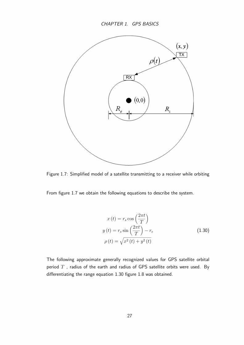
Figure 1.7 is a simplified model of satellite orbiting the Earth while transmittingto a receiver. No relativistic effects are considered and it is assumes that thesatellite’s orbit is perfectly circular with constant tangential velocity and when thesatellite is closest to the receiver the satellite is directly overhead.

26


Figure 1.7: Simplified model of a satellite transmitting to a receiver while orbiting

From figure 1.7 we obtain the following equations to describe the system.

x (t) = rs cos(2πtT

)y (t) = rs sin

(2πtT

)− re (1.30)

ρ (t) =√x2 (t) + y2 (t)

The following approximate generally recognized values for GPS satellite orbitalperiod T , radius of the earth and radius of GPS satellite orbits were used. Bydifferentiating the range equation 1.30 figure 1.8 was obtained.

27


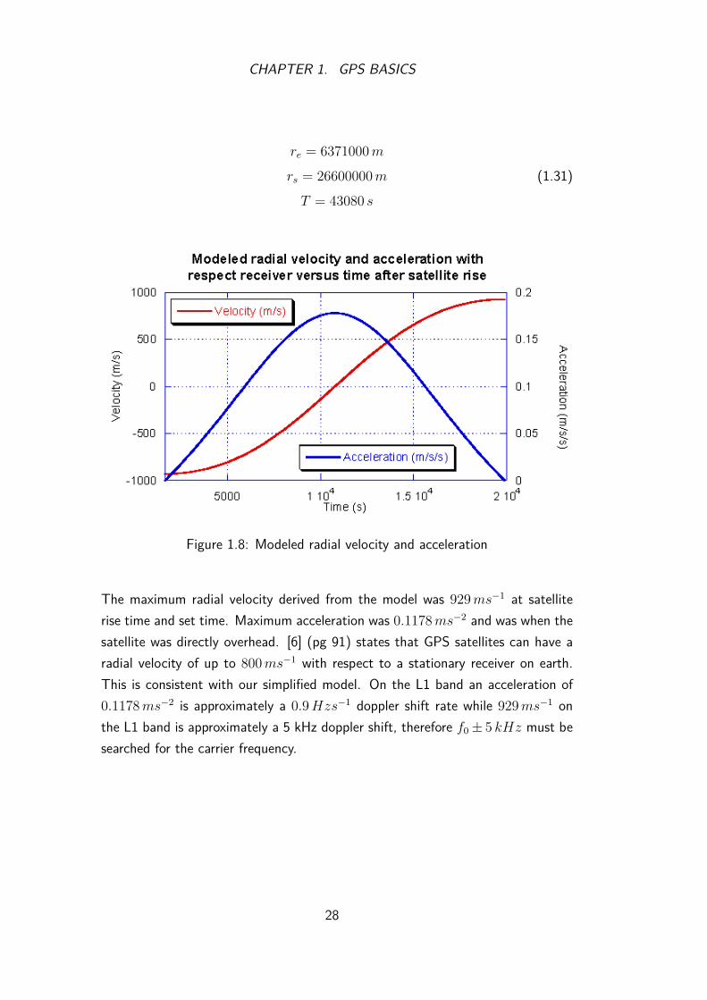
re = 6371000m

rs = 26600000m (1.31)

T = 43080 s

Figure 1.8: Modeled radial velocity and acceleration

The maximum radial velocity derived from the model was 929ms−1 at satelliterise time and set time. Maximum acceleration was 0.1178ms−2 and was when thesatellite was directly overhead. [6] (pg 91) states that GPS satellites can have aradial velocity of up to 800ms−1 with respect to a stationary receiver on earth.This is consistent with our simplified model. On the L1 band an acceleration of0.1178ms−2 is approximately a 0.9Hzs−1 doppler shift rate while 929ms−1 onthe L1 band is approximately a 5 kHz doppler shift, therefore f0± 5 kHz must besearched for the carrier frequency.

28

Nomenclature

2D two-dimensional

BPSK Binary Phase Shift Keying

C/A Coarse acquisition code

CDMA Code Division Multiple Access

Chip One bit of a PRN code

DLL Delay Locked Loop

FFT Fast Fourier Transform

FLL Frequency Locked Loop

GPS Global positioning system

HOW Hand Over Word

LS Least Squares

NAV Navigation Data

P Precise unencrypted code

PLL Phase Locked Loop

PRN Pseudo Random Number

RF Radio frequency

TEC Total Electron Count

UV UltraViolet

Y Precise encrypted code

29

Nomenclature

30

Bibliography

[1] Klobuchar, j.a. ionospheric effects on gps. gps world, April 1991. Vol. 2, No.4, pp. 48-51.

[2] Gps.gov: Gps modernization http://www.gps.gov/systems/gps/modernization/. Webpage, 2014. Modified: Monday, 15 September2014 12:53:11 p.m.

[3] Neo-7,u-blox 7, gnss modules data sheet. http://www.u-blox.com/images/downloads/Product_Docs/NEO-7_DataSheet_(GPS.G7-HW-11004).pdf,May 2014.

[4] Gruber, C. B. Gps modernization and program update. In Munich SatelliteNavigation Summit, Munich, Germany (2011).

[5] Klobuchar, J. Ionospheric time-delay algorithm for single-frequency gpsusers. Aerospace and Electronic Systems, IEEE Transactions on AES-23, 3(May 1987), 325–331.

[6] Van Diggelen, F. A-GPS: Assisted GPS, GNSS, and SBAS. Artech HouseGnss Technology and Applications Library. Artech House, 2009.

[7] Zhou, Y. Dsp in a satellite navigation receiver with a perspective of compu-tational complexity. Internet, Nov 2013.

31

http://www.gps.gov/systems/gps/modernization/

http://www.gps.gov/systems/gps/modernization/

http://www.u-blox.com/images/downloads/Product_Docs/NEO-7_DataSheet_(GPS.G7-HW-11004).pdf

http://www.u-blox.com/images/downloads/Product_Docs/NEO-7_DataSheet_(GPS.G7-HW-11004).pdf

Documents

Global Positioning System (GPS) Basics: Using GPS …jontio.zapto.org/hda1/gps-basics-jonti.pdf · 2015-09-02 · is in an eﬀort to upgrade the features and performance of GPS