Earth and Planetary Science Letters 431 (2015) 225–235

Contents lists available at ScienceDirect

Earth and Planetary Science Letters

www.elsevier.com/locate/epsl

Lithosphere–asthenosphere P-wave reflectivity across Australia

B.L.N. Kennett

Research School of Earth Sciences, The Australian National University, Canberra ACT 2601, Australia

a r t i c l e i n f o a b s t r a c t

Article history:Received 2 June 2015Received in revised form 22 September 2015Accepted 23 September 2015Available online xxxxEditor: P. Shearer

Keywords:Lithosphere–asthenosphere transitionmantle heterogeneityMoho

A direct image of P-wave reflectivity in the lithosphere and asthenosphere beneath seismic stations is extracted from stacked autocorrelograms of continuous component records. The autocorrelograms emphasise near vertically travelling waves, so that multiples are more muted than in receiver function studies and it is possible to work at higher frequencies than for receiver functions. Across a wide range of geological environments in Australia, in the 0.5–4.0 Hz frequency band, distinct reflections are seen in the crust underlain by weaker reflectivity in the lithosphere and asthenosphere. The base of crustal reflectivity fits well with Moho estimates from other classes of information. Few mantle reflectors have been seen in conventional reflection profiling at frequencies above 10 Hz; the presence of reflections in the 0.5–4.0 Hz band suggests variations on vertical scales of a few hundred metres with amplitudes of the order of 1%. There are slight indications of a change of reflection character in the lower part of the lithosphere in the transition to the asthenosphere. At a few stations there is a very clear lamination at asthenospheric depth, as well as reflections from the base of the S wave low velocity zone. Reflection bands often occur at depths where discontinuities have been inferred from S wave receiver function work at the same station, but would not by themselves be distinctive of a mid-lithosphere discontinuity.

© 2015 Elsevier B.V. All rights reserved.

1. Introduction

The complex configuration of the continental lithosphere and underlying asthenosphere has been the subject of a wide variety of studies using probes of many different types that emphasise different features. Much of the broad-scale knowledge comes from surface wave studies, with near horizontal wave propagation, at the global (e.g., Schaeffer and Lebedev, 2013) or regional scale (e.g., Yoshizawa, 2014 for Australia). In such surface-wave tomog-raphy the exploitation of large numbers of broad-band stations al-lows horizontal resolution of about 250 km with vertical resolution around 30 km. Surface wave studies can therefore map out the fast cratonic cores of continents, and indicate the depth where there is a transition to the lower wavespeed of the asthenosphere. Even were there to be a sharp discontinuity between the lithosphere and the asthenosphere, this would be imaged in surface-wave to-mography as a transition over about 30–40 km (Yoshizawa, 2014).

In contrast studies using body waves exploit arrivals at sta-tions from beneath, generally in a relatively narrow cone about the vertical. Tight horizontal resolution in tomographic work can be achieved with close station spacing, but vertical smearing and stretching of structure is inevitable because of the configuration of sampling (e.g., Rawlinson et al., 2014). Much effort has also

E-mail address: Brian.Kennett@anu.edu.au.

http://dx.doi.org/10.1016/j.epsl.2015.09.0390012-821X/© 2015 Elsevier B.V. All rights reserved.

been put into receiver function studies exploiting the conver-sions and reverberations accompanying the major seismic phases such as P or S from distant earthquakes (Langston, 1979; Vin-nik and Farra, 2000). For incident P waves, multiple crustal re-verberations tend to obscure conversions to S from contrasts at lithospheric and asthenospheric depth (Rychert et al., 2007). At-tention has therefore focused on incident S for which conver-sions to P outrun the S waves and arrive ahead of the main S phase, thereby avoiding overlap with crustal multiples. However, the lower frequencies of S mean that vertical resolution of the position and character of apparent discontinuities is limited, so that several minor changes may be conflated into a single fea-ture that is interpreted as a larger change in seismic wavespeeds (Selway et al., 2015). In particular S wave receiver function stud-ies have indicated the presence of an S wave velocity reduction at depths around 80-100 km, even in regions where other infor-mation suggests a generally fast lithosphere (e.g., Abt et al., 2010;Miller and Eaton, 2010; Ford et al., 2010). In the continents this feature is generally interpreted as a mid-lithospheric discontinuity (MLD), though there are dissenting views (e.g., Kind et al., 2012).

A further probe for investigating the lithosphere and astheno-sphere is provided by exploiting stacked autocorrelograms of the continuous traces at individual seismic stations. Building on results from Claerbout (1968), Gorbatov et al. (2013) have demonstrated that such station autocorrelograms provide a representation of the reflection sequence for near-vertical incidence waves at the station.

226 B.L.N. Kennett / Earth and Planetary Science Letters 431 (2015) 225–235

Tibuleac and von Seggern (2012) used ambient-noise autocorrelo-grams to map the depth of the very sharp Moho for the Basin and Range province in Nevada. Gorbatov et al. (2013) exploited sta-tions across Australia and showed that P-wave reflectivity could be extracted in a wide range of geological environments in the frequency range 2–4 Hz. The peak reflectivity does not always co-incide with the expected Moho mapped from the integration of a wide range of seismological information (Kennett et al., 2011). Gorbatov et al. (2013) noted a number of localities where signif-icant P wave reflections were returned from below the depth of the Moho, which were suggestive of reflectivity in the lithospheric mantle. At such frequencies the complex structures associated with the transition from crust to mantle frequently do not give any sim-ple signal associated with the Moho, unlike the distinctive pulse commonly seen in lower-frequency receiver function studies. Full-crustal reflection surveys have now been carried out across a wide range of geological regimes in Australia, from which Kennett and Saygin (2015) present a survey of the character of the reflection Moho across the continent; it is rare for the Moho at higher fre-quencies to be the most prominent crustal reflection.

In this study we exploit the station autocorrelograms across Australia, carried to later times, to look at the fine-scale struc-ture in the lithosphere and asthenosphere in a new way. In the frequency band 0.5–4.0 Hz we exploit P wavelengths of the order of 16–2 km in the uppermost mantle, so that features down to 0.25 km vertical scale could potentially be observed. The sampling is intrinsically vertical and so gives a different picture of the na-ture of the lithosphere from the studies of the detailed nature of the refracted field from Soviet peaceful-nuclear-explosions (PNE) in a similar frequency band undertaken by a number of authors (e.g., Tittgemeyer et al., 1996; Morozov et al., 1998; Nielsen et al., 2003).

Although the spatial intervals between available broadband sta-tions are quite large, the broad trends in lithosphere–asthenosphere reflectivity can be mapped across the whole Australian continent, and unprecedented details seen at a few stations.

2. Station autocorrelograms

The basic concept underlying the use of station autocorrelo-grams comes from work of Claerbout (1968) who showed that for an acoustic plane wave travelling vertically through a horizontally stratified medium the autocorrelation of the transmission response is equivalent to the reflection response, incorporating the effect of the free surface. Gorbatov et al. (2013) show how this con-cept extends to an elastic medium illuminated by distant events to give a local stacked reflection response. At the same time, for the ambient noise component, a station autocorrelogram can be viewed as the limit of cross-correlation between coincident sta-tions to give the zero-offset version of the Green’s function (cf. Poli et al., 2012). Thus two different conceptual approaches reinforce each other, and the entire continuous records can be used for au-tocorrelation. Vertical component records are used in this study, hence we will recover P-wave reflectivity beneath the stations.

Because the autocorrelograms of the noise component can be interpreted as representing the Green’s function for the case with coincident source and receiver, the resulting stack trace suffers the ambiguities inherent also in seismic reflection studies. The sig-nal is associated with a known two-way passage time, but the origin could correspond to anywhere on the isochronal surface, which will be roughly spherical in 3-D. We show below that the strong spatial coherence in stacked station autocorrelograms across closely spaced array stations provides good evidence for a dom-inant origin of the signal from vertically below the station. The conversion of transmitted P waves from earthquake signals into reflection traces via the autocorrelation process also helps to rein-force the depth component.

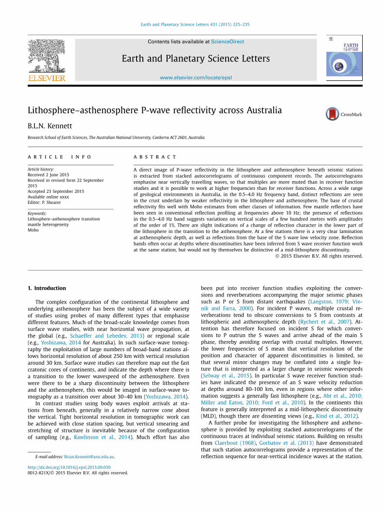
Fig. 1. Simplified representation of the main tectonic features of Australia. The out-line of the major cratons are marked by chain-dotted lines. The Tasman line in red is based on the reinterpretation by Direen and Crawford (2003). Key to marked features: AF – Albany-Fraser belt, Ar – Arunta Block, Am – Amadeus Basin, Ca – Can-ning basin, Cp – Capricorn Orogen, Cu – Curnamona Craton, Er – Eromanga basin,Eu – Eucla basin, Ga – Gawler craton, Ge – Georgetown inlier, Ha – Hamersley Basin, Ki – Kimberley block, La – Lachlan Orogen, Mc – MacArthur basin, MI – Mt Isa block, Mu – Musgrave block, NE – New England Orogen, Of – Officer basin,PC - Pine Creek Inlier, Pi - Pilbara craton, Pj - Pinjarra Orogen, T – Tennant Creek block, Yi – Yilgarn craton, NWS – Northwest Shelf, GBR – Great Barrier Reef, SD – Simpson Desert, GSD – Great Sandy Desert. Broad-band seismic stations across Aus-tralia for which station autocorrelograms have been constructed are indicated by filled diamonds. (For interpretation of the references to colour in this figure legend, the reader is referred to the web version of this article.)

Fig. 2. Broad-band seismic stations across Australia for which station autocorrel-ograms have been constructed are indicated by light-blue diamonds. Five profiles are marked for which detailed results are displayed in Figs. 6–10. Profiles A and B cross multiple age provinces, whereas profiles C, D and E lie largely within a sin-gle province. The configuration of the major Precambrian cratons (WA, NA, SA) and the Tasman Line (TL) from Fig. 1 are also indicated. (For interpretation of the ref-erences to colour in this figure legend, the reader is referred to the web version of this article.)

Stacked autocorrelogram traces have been constructed for all the broad-band stations across Australia (Figs. 1, 2) using 6 h con-tiguous windows from the vertical component. Stations with data gaps or spikes, related to instrumental problems, have been re-

B.L.N. Kennett / Earth and Planetary Science Letters 431 (2015) 225–235 227

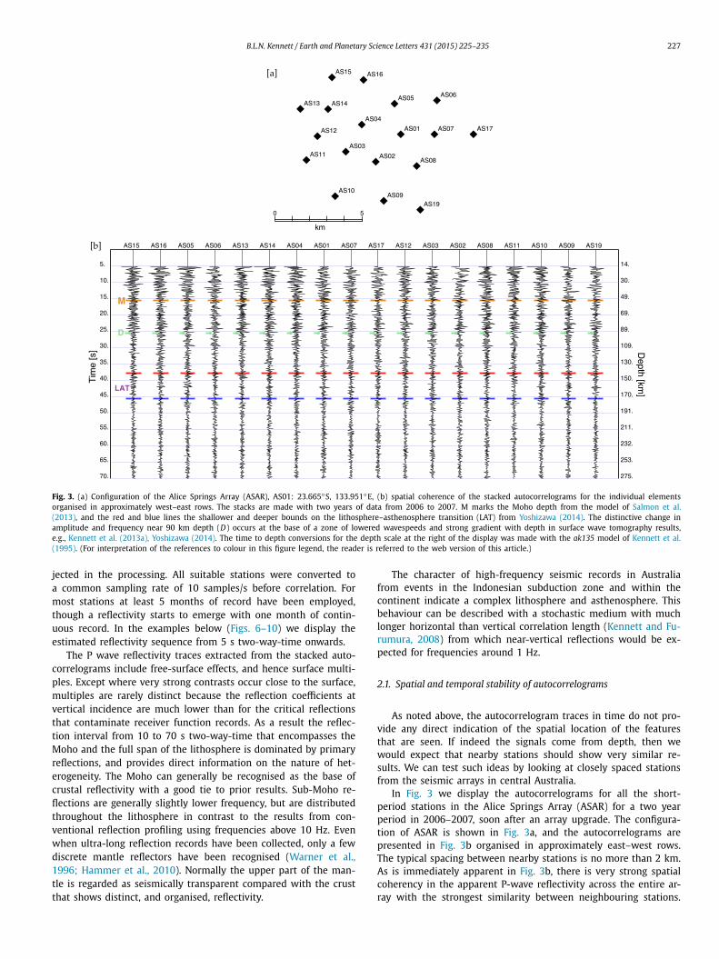
Fig. 3. (a) Configuration of the Alice Springs Array (ASAR), AS01: 23.665◦S, 133.951◦E, (b) spatial coherence of the stacked autocorrelograms for the individual elements organised in approximately west–east rows. The stacks are made with two years of data from 2006 to 2007. M marks the Moho depth from the model of Salmon et al. (2013), and the red and blue lines the shallower and deeper bounds on the lithosphere–asthenosphere transition (LAT) from Yoshizawa (2014). The distinctive change in amplitude and frequency near 90 km depth (D) occurs at the base of a zone of lowered wavespeeds and strong gradient with depth in surface wave tomography results, e.g., Kennett et al. (2013a), Yoshizawa (2014). The time to depth conversions for the depth scale at the right of the display was made with the ak135 model of Kennett et al. (1995). (For interpretation of the references to colour in this figure legend, the reader is referred to the web version of this article.)

jected in the processing. All suitable stations were converted to a common sampling rate of 10 samples/s before correlation. For most stations at least 5 months of record have been employed, though a reflectivity starts to emerge with one month of contin-uous record. In the examples below (Figs. 6–10) we display the estimated reflectivity sequence from 5 s two-way-time onwards.

The P wave reflectivity traces extracted from the stacked auto-correlograms include free-surface effects, and hence surface multi-ples. Except where very strong contrasts occur close to the surface, multiples are rarely distinct because the reflection coefficients at vertical incidence are much lower than for the critical reflections that contaminate receiver function records. As a result the reflec-tion interval from 10 to 70 s two-way-time that encompasses the Moho and the full span of the lithosphere is dominated by primary reflections, and provides direct information on the nature of het-erogeneity. The Moho can generally be recognised as the base of crustal reflectivity with a good tie to prior results. Sub-Moho re-flections are generally slightly lower frequency, but are distributed throughout the lithosphere in contrast to the results from con-ventional reflection profiling using frequencies above 10 Hz. Even when ultra-long reflection records have been collected, only a few discrete mantle reflectors have been recognised (Warner et al., 1996; Hammer et al., 2010). Normally the upper part of the man-tle is regarded as seismically transparent compared with the crust that shows distinct, and organised, reflectivity.

The character of high-frequency seismic records in Australia from events in the Indonesian subduction zone and within the continent indicate a complex lithosphere and asthenosphere. This behaviour can be described with a stochastic medium with much longer horizontal than vertical correlation length (Kennett and Fu-rumura, 2008) from which near-vertical reflections would be ex-pected for frequencies around 1 Hz.

2.1. Spatial and temporal stability of autocorrelograms

As noted above, the autocorrelogram traces in time do not pro-vide any direct indication of the spatial location of the features that are seen. If indeed the signals come from depth, then we would expect that nearby stations should show very similar re-sults. We can test such ideas by looking at closely spaced stations from the seismic arrays in central Australia.

In Fig. 3 we display the autocorrelograms for all the short-period stations in the Alice Springs Array (ASAR) for a two year period in 2006–2007, soon after an array upgrade. The configura-tion of ASAR is shown in Fig. 3a, and the autocorrelograms are presented in Fig. 3b organised in approximately east–west rows. The typical spacing between nearby stations is no more than 2 km. As is immediately apparent in Fig. 3b, there is very strong spatial coherency in the apparent P-wave reflectivity across the entire ar-ray with the strongest similarity between neighbouring stations.

228 B.L.N. Kennett / Earth and Planetary Science Letters 431 (2015) 225–235

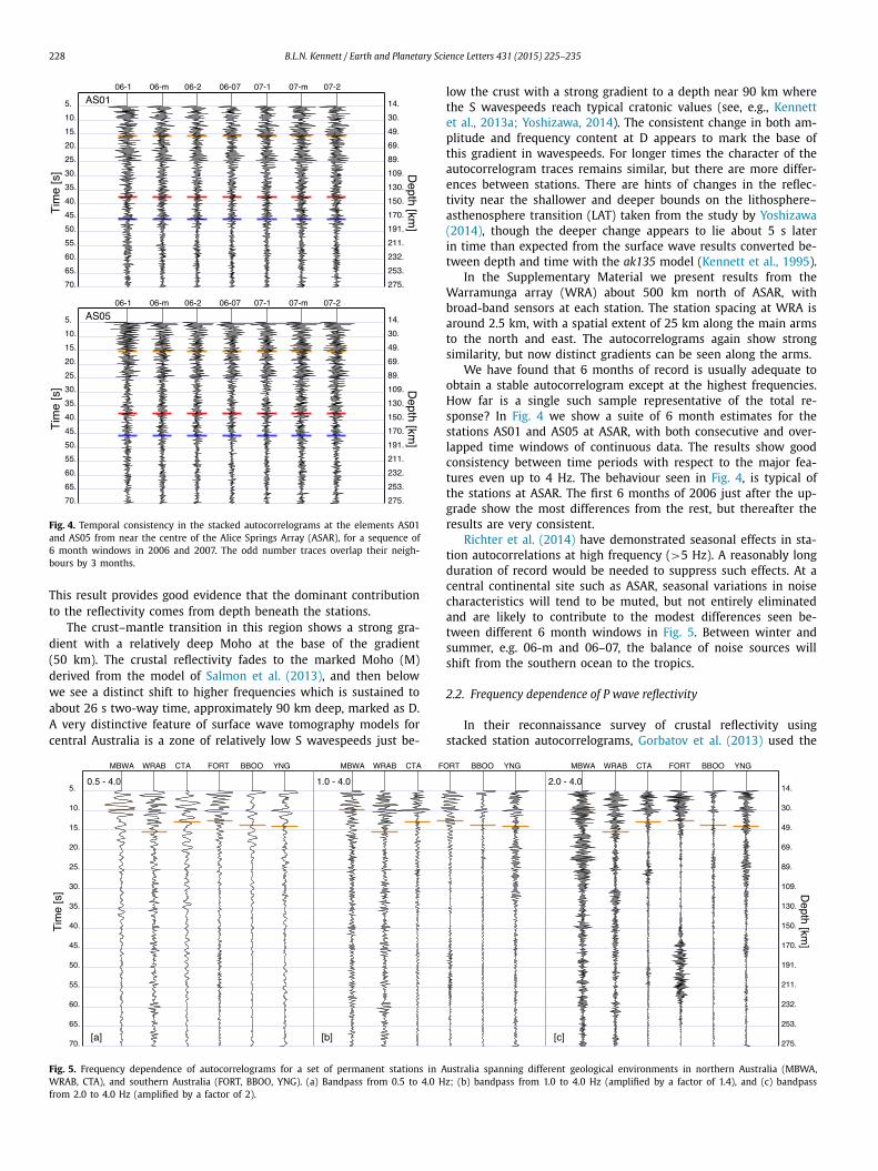
Fig. 4. Temporal consistency in the stacked autocorrelograms at the elements AS01 and AS05 from near the centre of the Alice Springs Array (ASAR), for a sequence of 6 month windows in 2006 and 2007. The odd number traces overlap their neigh-bours by 3 months.

This result provides good evidence that the dominant contribution to the reflectivity comes from depth beneath the stations.

The crust–mantle transition in this region shows a strong gra-dient with a relatively deep Moho at the base of the gradient (50 km). The crustal reflectivity fades to the marked Moho (M) derived from the model of Salmon et al. (2013), and then below we see a distinct shift to higher frequencies which is sustained to about 26 s two-way time, approximately 90 km deep, marked as D. A very distinctive feature of surface wave tomography models for central Australia is a zone of relatively low S wavespeeds just be-

low the crust with a strong gradient to a depth near 90 km where the S wavespeeds reach typical cratonic values (see, e.g., Kennett et al., 2013a; Yoshizawa, 2014). The consistent change in both am-plitude and frequency content at D appears to mark the base of this gradient in wavespeeds. For longer times the character of the autocorrelogram traces remains similar, but there are more differ-ences between stations. There are hints of changes in the reflec-tivity near the shallower and deeper bounds on the lithosphere–asthenosphere transition (LAT) taken from the study by Yoshizawa(2014), though the deeper change appears to lie about 5 s later in time than expected from the surface wave results converted be-tween depth and time with the ak135 model (Kennett et al., 1995).

In the Supplementary Material we present results from the Warramunga array (WRA) about 500 km north of ASAR, with broad-band sensors at each station. The station spacing at WRA is around 2.5 km, with a spatial extent of 25 km along the main arms to the north and east. The autocorrelograms again show strong similarity, but now distinct gradients can be seen along the arms.

We have found that 6 months of record is usually adequate to obtain a stable autocorrelogram except at the highest frequencies. How far is a single such sample representative of the total re-sponse? In Fig. 4 we show a suite of 6 month estimates for the stations AS01 and AS05 at ASAR, with both consecutive and over-lapped time windows of continuous data. The results show good consistency between time periods with respect to the major fea-tures even up to 4 Hz. The behaviour seen in Fig. 4, is typical of the stations at ASAR. The first 6 months of 2006 just after the up-grade show the most differences from the rest, but thereafter the results are very consistent.

Richter et al. (2014) have demonstrated seasonal effects in sta-tion autocorrelations at high frequency (>5 Hz). A reasonably long duration of record would be needed to suppress such effects. At a central continental site such as ASAR, seasonal variations in noise characteristics will tend to be muted, but not entirely eliminated and are likely to contribute to the modest differences seen be-tween different 6 month windows in Fig. 5. Between winter and summer, e.g. 06-m and 06–07, the balance of noise sources will shift from the southern ocean to the tropics.

2.2. Frequency dependence of P wave reflectivity

In their reconnaissance survey of crustal reflectivity using stacked station autocorrelograms, Gorbatov et al. (2013) used the

Fig. 5. Frequency dependence of autocorrelograms for a set of permanent stations in Australia spanning different geological environments in northern Australia (MBWA, WRAB, CTA), and southern Australia (FORT, BBOO, YNG). (a) Bandpass from 0.5 to 4.0 Hz; (b) bandpass from 1.0 to 4.0 Hz (amplified by a factor of 1.4), and (c) bandpass from 2.0 to 4.0 Hz (amplified by a factor of 2).

B.L.N. Kennett / Earth and Planetary Science Letters 431 (2015) 225–235 229

frequency band from 2.0 to 4.0 Hz. Such traces are quite effective for purely crustal studies (Kennett et al., in press), but the fre-quency choice may obscure the overall character at later times for which energy may be reflected from fine structure in the lithosphere and asthenosphere. The crustal response is normally clearest when the frequency threshold is 1 Hz or above.

In Fig. 5 we show results on the frequency dependence of the stacked autocorrelograms from six permanent stations distributed across Australia in different geological environments. In the north-ern group MBWA lies on the Archean Pilbara of Western Australia, WRAB in the Proterozoic of the North Australian craton, and CTA in the Phanerozoic of eastern Australia. FORT in the southern group is on presumed Proterozoic material, obscured by thick cover, BBOO on the Gawler component of the South Australian craton, most likely Archean, and YNG in the Paleozoic Lachlan Fold Belt. For each station we show the autocorrelogram traces filtered in the with frequency bands 0.5–4.0 Hz, 1.0–4.0 Hz, and 2.0–4.0 Hz. The tighter bands are amplified somewhat to allow the traces to be clearly seen.

The dominant longer period response at MBWA hides a sub-stantial contribution from higher frequencies, but there is good alignment in the times where the character of the apparent re-flectivity at later times changes The crustal transition at MBWA is most clear in the 1.0–4.0 Hz band. In contrast, at WRAB we have substantial higher frequencies in the autocorrelogram which are still evident in the broadest band. The stations FORT and CTA show distinct high frequency trains at later times that, as we shall see, tie well with other information about structure.

The results for the broadest frequency band 0.5–4.0 Hz are not too cluttered with apparent arrivals, but still allow strong changes in frequency character such as that at FORT near 40 s to be iden-tified without being overwhelmed by rapid or noisy variations. This is the preferred frequency window for all permanent sta-tion results. However, for temporary deployments – whose station names end in numbers – we have used the more restricted band 0.6-2.0 Hz. Such portable stations have highly variable emplace-ment conditions, and the shorter duration of deployment means that there is less cancellation of high frequency noise, and this tends to contaminate the traces for times corresponds to returns from below the Moho.

2.3. Autocorrelograms and other lithospheric analysis tools

Kennett et al. (in press) have demonstrated how station auto-correlograms from the dense deployments of seismic stations in southeastern Australia can be exploited to enhance spatial cover-age of the depth to Moho, including the use of older data which cannot be used for receiver function studies because only verti-cal component recordings are available. Spatial stacks of crustal P wave reflectivity derived from autocorrelograms at over 750 sta-tions, in the 2–4 Hz band, were created at 180 locations using a Gaussian with half-width 0.5◦ . In many parts of this region the transition from crust to mantle is gradational, and so there is often no distinct reflector to correspond to the Moho. Instead it is neces-sary to seek the base of the crustal reflectivity, a process that was aided by the use of the Moho model of Salmon et al. (2013) based on sparser data.

The current seismological tools which are available to interro-gate the structure of the lithospheric mantle and asthenosphere come in two classes. First, methods that exploit near-horizontal wave propagation as in the analysis of fundamental and higher mode surface waves, that have the strongest dependence on S wavespeed. Generally such waves are exploited to no higher fre-quency than 0.05 Hz so that vertical resolution is limited to 25 km at best. Even when full waveform inversion is employed in 3-D (e.g. Fichtner et al., 2009) fine-scale structure will be heavily av-

eraged and only aggregate properties can be extracted. Second, methods exploiting steeply arriving seismic waves from distant such receiver function methods. Because of the interference of crustal multiples with lithospheric signals for incident P aves, S-wave receiver functions have been extensively used to examine lithospheric discontinuities (e.g., Ford et al., 2010). Analysis is made at relatively low frequencies, typically 0.1–0.2 Hz, and the method depends on conversion from contrasts in S wavespeed structure. Arrivals associated with the mid-lithosphere discon-tinuity, and the lithosphere-boundary, are likely to arise from the interaction of many smaller structures (e.g., Selway et al., 2015).

The station autocorrelogram approach exploits transmitted waves and ambient noise, with dominant sensitivity to P wave impedance contrast. With the frequency ranges we have used, structures as small as 0.5 km in vertical extent could have an influ-ence. This is the estimated vertical correlation length in stochastic models for the cratonic lithosphere in northern Australia found from the properties of high-frequency waves from events in the Indonesian Subduction zone (Kennett and Furumura, 2008). The autocorrelogram approach thus bridges a gap between determinis-tic models using longer wavelength waves and stochastic models at high frequency. Because the wavelengths used are much shorter, we cannot expect direct correspondence with the features recog-nised using longer-period waves, but may be able to recognise changes in fine-scale structure that are linked to the macroscopic discontinuities. Large-scale variations in P wavespeed in the litho-spheric mantle across Australia are generally about one-third or less of the S wavespeed variation (Kennett et al., 2013a). We simply do not know whether such behaviour persists to finer scale, but we have to allow for the possibility that the actual P wave reflectivity is quite small and so results may be natu-rally quite noisy. Further we cannot exclude the possibility of contamination by “side-wipe” from structures which are not at depth. We therefore have to be careful not to over-interpret the results.

3. P wave reflectivity across Australia

Station autocorrelograms for up to 70 s lag have been extracted for all stations considered by Gorbatov et al. (2013), supplemented by some recently deployed portable broadband stations (Fig. 1). The stations cover the full range of geological environments in Aus-tralia, with ages from Archean to Paleozoic.

In order to tie with previous results, particularly the S wave receiver function study of Ford et al. (2010), we have extracted five profiles of stations including both permanent sites and tem-porary deployments (Fig. 2). The west–east profiles A and B cover the full span of crustal ages, whilst the north–south profiles C, D and E largely lie within a single age zone. The broad-band stations are broadly spaced across the continent and so we cannot expect to find lateral continuity of structure. Instead we can anticipate contrasts in properties between stations in different geological en-vironments. As far as possible we display the records with true relative amplitudes, but have had to make some allowance for strong site effects at the portable stations.

The relatively sparse spacing of the available stations means that we focus on the major differences between the lithosphere associated with different tectonic units, and will see that we can distinguish some age dependent properties.

3.1. Profile A

Profile A approximately follows latitude 20◦S, and so in Fig. 6we illustrate the S wavespeed from the isotropic model of Yoshiza-wa (2014) with the projection of the stations at the appropriate

230 B.L.N. Kennett / Earth and Planetary Science Letters 431 (2015) 225–235

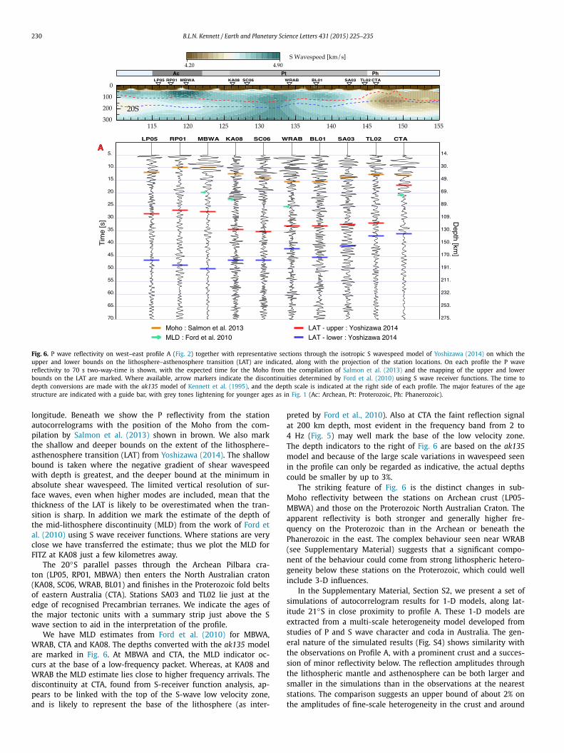
Fig. 6. P wave reflectivity on west–east profile A (Fig. 2) together with representative sections through the isotropic S wavespeed model of Yoshizawa (2014) on which the upper and lower bounds on the lithosphere–asthenosphere transition (LAT) are indicated, along with the projection of the station locations. On each profile the P wave reflectivity to 70 s two-way-time is shown, with the expected time for the Moho from the compilation of Salmon et al. (2013) and the mapping of the upper and lower bounds on the LAT are marked. Where available, arrow markers indicate the discontinuities determined by Ford et al. (2010) using S wave receiver functions. The time to depth conversions are made with the ak135 model of Kennett et al. (1995), and the depth scale is indicated at the right side of each profile. The major features of the age structure are indicated with a guide bar, with grey tones lightening for younger ages as in Fig. 1 (Ac: Archean, Pt: Proterozoic, Ph: Phanerozoic).

longitude. Beneath we show the P reflectivity from the station autocorrelograms with the position of the Moho from the com-pilation by Salmon et al. (2013) shown in brown. We also mark the shallow and deeper bounds on the extent of the lithosphere–asthenosphere transition (LAT) from Yoshizawa (2014). The shallow bound is taken where the negative gradient of shear wavespeed with depth is greatest, and the deeper bound at the minimum in absolute shear wavespeed. The limited vertical resolution of sur-face waves, even when higher modes are included, mean that the thickness of the LAT is likely to be overestimated when the tran-sition is sharp. In addition we mark the estimate of the depth of the mid-lithosphere discontinuity (MLD) from the work of Ford et al. (2010) using S wave receiver functions. Where stations are very close we have transferred the estimate; thus we plot the MLD for FITZ at KA08 just a few kilometres away.

The 20◦S parallel passes through the Archean Pilbara cra-ton (LP05, RP01, MBWA) then enters the North Australian craton (KA08, SC06, WRAB, BL01) and finishes in the Proterozoic fold belts of eastern Australia (CTA). Stations SA03 and TL02 lie just at the edge of recognised Precambrian terranes. We indicate the ages of the major tectonic units with a summary strip just above the S wave section to aid in the interpretation of the profile.

We have MLD estimates from Ford et al. (2010) for MBWA, WRAB, CTA and KA08. The depths converted with the ak135 model are marked in Fig. 6. At MBWA and CTA, the MLD indicator oc-curs at the base of a low-frequency packet. Whereas, at KA08 and WRAB the MLD estimate lies close to higher frequency arrivals. The discontinuity at CTA, found from S-receiver function analysis, ap-pears to be linked with the top of the S-wave low velocity zone, and is likely to represent the base of the lithosphere (as inter-

preted by Ford et al., 2010). Also at CTA the faint reflection signal at 200 km depth, most evident in the frequency band from 2 to 4 Hz (Fig. 5) may well mark the base of the low velocity zone. The depth indicators to the right of Fig. 6 are based on the ak135model and because of the large scale variations in wavespeed seen in the profile can only be regarded as indicative, the actual depths could be smaller by up to 3%.

The striking feature of Fig. 6 is the distinct changes in sub-Moho reflectivity between the stations on Archean crust (LP05-MBWA) and those on the Proterozoic North Australian Craton. The apparent reflectivity is both stronger and generally higher fre-quency on the Proterozoic than in the Archean or beneath the Phanerozoic in the east. The complex behaviour seen near WRAB (see Supplementary Material) suggests that a significant compo-nent of the behaviour could come from strong lithospheric hetero-geneity below these stations on the Proterozoic, which could well include 3-D influences.

In the Supplementary Material, Section S2, we present a set of simulations of autocorrelogram results for 1-D models, along lat-itude 21◦S in close proximity to profile A. These 1-D models are extracted from a multi-scale heterogeneity model developed from studies of P and S wave character and coda in Australia. The gen-eral nature of the simulated results (Fig. S4) shows similarity with the observations on Profile A, with a prominent crust and a succes-sion of minor reflectivity below. The reflection amplitudes through the lithospheric mantle and asthenosphere can be both larger and smaller in the simulations than in the observations at the nearest stations. The comparison suggests an upper bound of about 2% on the amplitudes of fine-scale heterogeneity in the crust and around

B.L.N. Kennett / Earth and Planetary Science Letters 431 (2015) 225–235 231

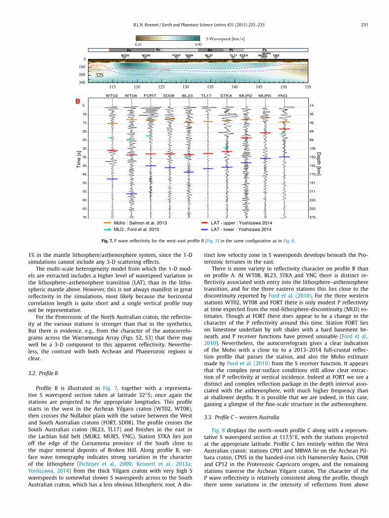
Fig. 7. P wave reflectivity for the west–east profile B (Fig. 2) in the same configuration as in Fig. 6.

1% in the mantle lithosphere/asthenosphere system, since the 1-D simulations cannot include any 3-D scattering effects.

The multi-scale heterogeneity model from which the 1-D mod-els are extracted includes a higher level of wavespeed variation in the lithosphere–asthenosphere transition (LAT), than in the litho-spheric mantle above. However, this is not always manifest in great reflectivity in the simulations, most likely because the horizontal correlation length is quite short and a single vertical profile may not be representative.

For the Proterozoic of the North Australian craton, the reflectiv-ity at the various stations is stronger than that in the synthetics, But there is evidence, e.g., from the character of the autocorrelo-grams across the Warramunga Array (Figs. S2, S3) that there may well be a 3-D component to this apparent reflectivity. Neverthe-less, the contrast with both Archean and Phanerozoic regions is clear.

3.2. Profile B

Profile B is illustrated in Fig. 7, together with a representa-tive S wavespeed section taken at latitude 32◦S; once again the stations are projected to the appropriate longitudes. This profile starts in the west in the Archean Yilgarn craton (WT02, WT08), then crosses the Nullabor plain with the suture between the West and South Australian cratons (FORT, SD08). The profile crosses the South Australian craton (BL23, TL17) and finishes in the east in the Lachlan fold belt (MUR2, MUR5, YNG). Station STKA lies just off the edge of the Curnamona province of the South close to the major mineral deposits of Broken Hill. Along profile B, sur-face wave tomography indicates strong variation in the character of the lithosphere (Fichtner et al., 2009; Kennett et al., 2013a;Yoshizawa, 2014) from the thick Yilgarn craton with very high S wavespeeds to somewhat slower S wavespeeds across to the South Australian craton, which has a less obvious lithospheric root. A dis-

tinct low velocity zone in S wavespeeds develops beneath the Pro-terozoic terranes in the east.

There is more variety in reflectivity character on profile B than on profile A. At WT08, BL23, STKA and YNG there is distinct re-flectivity associated with entry into the lithosphere–asthenosphere transition, and for the three eastern stations this lies close to the discontinuity reported by Ford et al. (2010). For the three western stations WT02, WT08 and FORT there is only modest P reflectivity at time expected from the mid-lithosphere-discontinuity (MLD) es-timates. Though at FORT there does appear to be a change in the character of the P reflectivity around this time. Station FORT lies on limestone underlain by soft shales with a hard basement be-neath, and P receiver functions have proved unusable (Ford et al., 2010). Nevertheless, the autocorrelogram gives a clear indication of the Moho with a close tie to a 2013–2014 full-crustal reflec-tion profile that passes the station, and also the Moho estimate made by Ford et al. (2010) from the S receiver function. It appears that the complex near-surface conditions still allow clear extrac-tion of P reflectivity at vertical incidence. Indeed at FORT we see a distinct and complex reflection package in the depth interval asso-ciated with the asthenosphere, with much higher frequency than at shallower depths. It is possible that we are indeed, in this case, gaining a glimpse of the fine-scale structure in the asthenosphere.

3.3. Profile C – western Australia

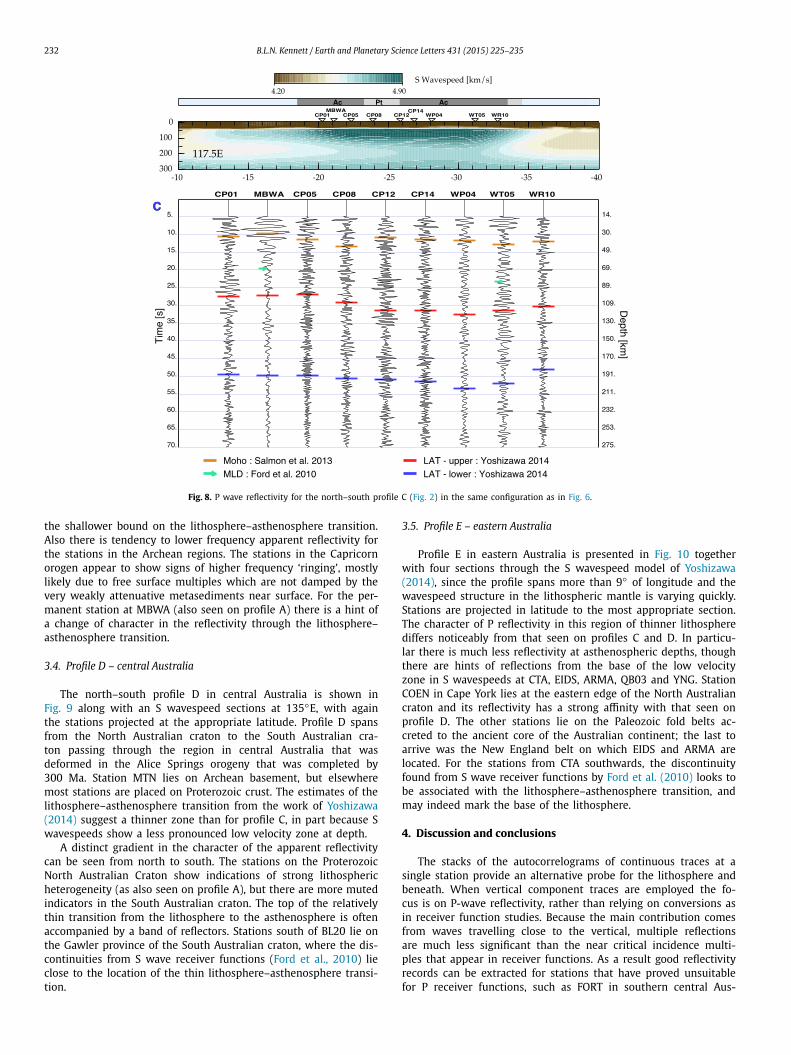
Fig. 8 displays the north–south profile C along with a represen-tative S wavespeed section at 117.5◦E, with the stations projected at the appropriate latitude. Profile C lies entirely within the West Australian craton; stations CP01 and MBWA lie on the Archean Pil-bara craton, CP05 in the banded-iron rich Hammersley Basin, CP08 and CP12 in the Proterozoic Capricorn orogen, and the remaining stations traverse the Archean Yilgarn craton. The character of the P wave reflectivity is relatively consistent along the profile, though there some variations in the intensity of reflections from above

232 B.L.N. Kennett / Earth and Planetary Science Letters 431 (2015) 225–235

Fig. 8. P wave reflectivity for the north–south profile C (Fig. 2) in the same configuration as in Fig. 6.

the shallower bound on the lithosphere–asthenosphere transition. Also there is tendency to lower frequency apparent reflectivity for the stations in the Archean regions. The stations in the Capricorn orogen appear to show signs of higher frequency ‘ringing’, mostly likely due to free surface multiples which are not damped by the very weakly attenuative metasediments near surface. For the per-manent station at MBWA (also seen on profile A) there is a hint of a change of character in the reflectivity through the lithosphere–asthenosphere transition.

3.4. Profile D – central Australia

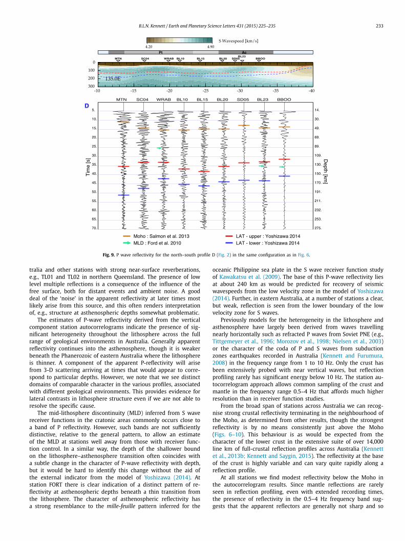
The north–south profile D in central Australia is shown in Fig. 9 along with an S wavespeed sections at 135◦E, with again the stations projected at the appropriate latitude. Profile D spans from the North Australian craton to the South Australian cra-ton passing through the region in central Australia that was deformed in the Alice Springs orogeny that was completed by 300 Ma. Station MTN lies on Archean basement, but elsewhere most stations are placed on Proterozoic crust. The estimates of the lithosphere–asthenosphere transition from the work of Yoshizawa(2014) suggest a thinner zone than for profile C, in part because S wavespeeds show a less pronounced low velocity zone at depth.

A distinct gradient in the character of the apparent reflectivity can be seen from north to south. The stations on the Proterozoic North Australian Craton show indications of strong lithospheric heterogeneity (as also seen on profile A), but there are more muted indicators in the South Australian craton. The top of the relatively thin transition from the lithosphere to the asthenosphere is often accompanied by a band of reflectors. Stations south of BL20 lie on the Gawler province of the South Australian craton, where the dis-continuities from S wave receiver functions (Ford et al., 2010) lie close to the location of the thin lithosphere–asthenosphere transi-tion.

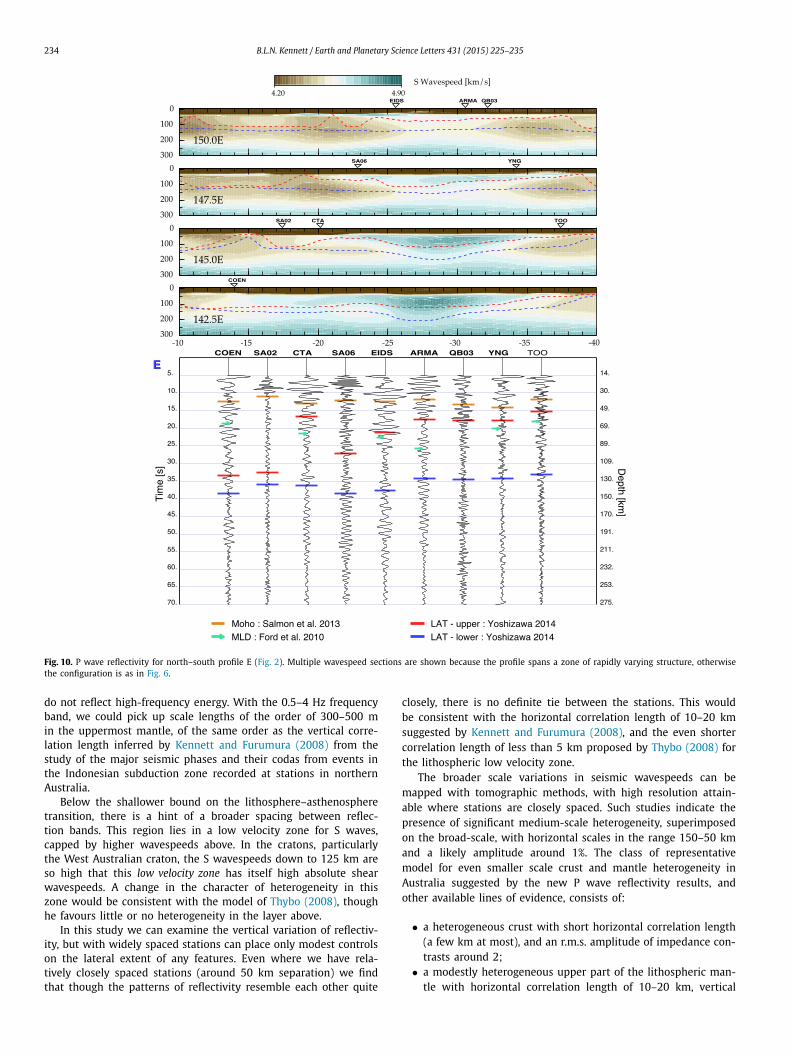
3.5. Profile E – eastern Australia

Profile E in eastern Australia is presented in Fig. 10 together with four sections through the S wavespeed model of Yoshizawa(2014), since the profile spans more than 9◦ of longitude and the wavespeed structure in the lithospheric mantle is varying quickly. Stations are projected in latitude to the most appropriate section. The character of P reflectivity in this region of thinner lithosphere differs noticeably from that seen on profiles C and D. In particu-lar there is much less reflectivity at asthenospheric depths, though there are hints of reflections from the base of the low velocity zone in S wavespeeds at CTA, EIDS, ARMA, QB03 and YNG. Station COEN in Cape York lies at the eastern edge of the North Australian craton and its reflectivity has a strong affinity with that seen on profile D. The other stations lie on the Paleozoic fold belts ac-creted to the ancient core of the Australian continent; the last to arrive was the New England belt on which EIDS and ARMA are located. For the stations from CTA southwards, the discontinuity found from S wave receiver functions by Ford et al. (2010) looks to be associated with the lithosphere–asthenosphere transition, and may indeed mark the base of the lithosphere.

4. Discussion and conclusions

The stacks of the autocorrelograms of continuous traces at a single station provide an alternative probe for the lithosphere and beneath. When vertical component traces are employed the fo-cus is on P-wave reflectivity, rather than relying on conversions as in receiver function studies. Because the main contribution comes from waves travelling close to the vertical, multiple reflections are much less significant than the near critical incidence multi-ples that appear in receiver functions. As a result good reflectivity records can be extracted for stations that have proved unsuitable for P receiver functions, such as FORT in southern central Aus-

B.L.N. Kennett / Earth and Planetary Science Letters 431 (2015) 225–235 233

Fig. 9. P wave reflectivity for the north–south profile D (Fig. 2) in the same configuration as in Fig. 6.

tralia and other stations with strong near-surface reverberations, e.g., TL01 and TL02 in northern Queensland. The presence of low level multiple reflections is a consequence of the influence of the free surface, both for distant events and ambient noise. A good deal of the ‘noise’ in the apparent reflectivity at later times most likely arise from this source, and this often renders interpretation of, e.g., structure at asthenospheric depths somewhat problematic.

The estimates of P-wave reflectivity derived from the vertical component station autocorrelograms indicate the presence of sig-nificant heterogeneity throughout the lithosphere across the full range of geological environments in Australia. Generally apparent reflectivity continues into the asthenosphere, though it is weaker beneath the Phanerozoic of eastern Australia where the lithosphere is thinner. A component of the apparent P-reflectivity will arise from 3-D scattering arriving at times that would appear to corre-spond to particular depths. However, we note that we see distinct domains of comparable character in the various profiles, associated with different geological environments. This provides evidence for lateral contrasts in lithosphere structure even if we are not able to resolve the specific cause.

The mid-lithosphere discontinuity (MLD) inferred from S wave receiver functions in the cratonic areas commonly occurs close to a band of P reflectivity. However, such bands are not sufficiently distinctive, relative to the general pattern, to allow an estimate of the MLD at stations well away from those with receiver func-tion control. In a similar way, the depth of the shallower bound on the lithosphere–asthenosphere transition often coincides with a subtle change in the character of P-wave reflectivity with depth, but it would be hard to identify this change without the aid of the external indicator from the model of Yoshizawa (2014). At station FORT there is clear indication of a distinct pattern of re-flectivity at asthenospheric depths beneath a thin transition from the lithosphere. The character of asthenospheric reflectivity has a strong resemblance to the mille-feuille pattern inferred for the

oceanic Philippine sea plate in the S wave receiver function study of Kawakatsu et al. (2009). The base of this P-wave reflectivity lies at about 240 km as would be predicted for recovery of seismic wavespeeds from the low velocity zone in the model of Yoshizawa(2014). Further, in eastern Australia, at a number of stations a clear, but weak, reflection is seen from the lower boundary of the low velocity zone for S waves.

Previously models for the heterogeneity in the lithosphere and asthenosphere have largely been derived from waves travelling nearly horizontally such as refracted P waves from Soviet PNE (e.g., Tittgemeyer et al., 1996; Morozov et al., 1998; Nielsen et al., 2003) or the character of the coda of P and S waves from subduction zones earthquakes recorded in Australia (Kennett and Furumura, 2008) in the frequency range from 1 to 10 Hz. Only the crust has been extensively probed with near vertical waves, but reflection profiling rarely has significant energy below 10 Hz. The station au-tocorrelogram approach allows common sampling of the crust and mantle in the frequency range 0.5–4 Hz that affords much higher resolution than in receiver function studies.

From the broad span of stations across Australia we can recog-nise strong crustal reflectivity terminating in the neighbourhood of the Moho, as determined from other results, though the strongest reflectivity is by no means consistently just above the Moho (Figs. 6–10). This behaviour is as would be expected from the character of the lower crust in the extensive suite of over 14,000 line km of full-crustal reflection profiles across Australia (Kennett et al., 2013b; Kennett and Saygin, 2015). The reflectivity at the base of the crust is highly variable and can vary quite rapidly along a reflection profile.

At all stations we find modest reflectivity below the Moho in the autocorrelogram results. Since mantle reflections are rarely seen in reflection profiling, even with extended recording times, the presence of reflectivity in the 0.5–4 Hz frequency band sug-gests that the apparent reflectors are generally not sharp and so

234 B.L.N. Kennett / Earth and Planetary Science Letters 431 (2015) 225–235

Fig. 10. P wave reflectivity for north–south profile E (Fig. 2). Multiple wavespeed sections are shown because the profile spans a zone of rapidly varying structure, otherwise the configuration is as in Fig. 6.

do not reflect high-frequency energy. With the 0.5–4 Hz frequency band, we could pick up scale lengths of the order of 300–500 m in the uppermost mantle, of the same order as the vertical corre-lation length inferred by Kennett and Furumura (2008) from the study of the major seismic phases and their codas from events in the Indonesian subduction zone recorded at stations in northern Australia.

Below the shallower bound on the lithosphere–asthenosphere transition, there is a hint of a broader spacing between reflec-tion bands. This region lies in a low velocity zone for S waves, capped by higher wavespeeds above. In the cratons, particularly the West Australian craton, the S wavespeeds down to 125 km are so high that this low velocity zone has itself high absolute shear wavespeeds. A change in the character of heterogeneity in this zone would be consistent with the model of Thybo (2008), though he favours little or no heterogeneity in the layer above.

In this study we can examine the vertical variation of reflectiv-ity, but with widely spaced stations can place only modest controls on the lateral extent of any features. Even where we have rela-tively closely spaced stations (around 50 km separation) we find that though the patterns of reflectivity resemble each other quite

closely, there is no definite tie between the stations. This would be consistent with the horizontal correlation length of 10–20 km suggested by Kennett and Furumura (2008), and the even shorter correlation length of less than 5 km proposed by Thybo (2008) for the lithospheric low velocity zone.

The broader scale variations in seismic wavespeeds can be mapped with tomographic methods, with high resolution attain-able where stations are closely spaced. Such studies indicate the presence of significant medium-scale heterogeneity, superimposed on the broad-scale, with horizontal scales in the range 150–50 km and a likely amplitude around 1%. The class of representative model for even smaller scale crust and mantle heterogeneity in Australia suggested by the new P wave reflectivity results, and other available lines of evidence, consists of:

• a heterogeneous crust with short horizontal correlation length (a few km at most), and an r.m.s. amplitude of impedance con-trasts around 2;

• a modestly heterogeneous upper part of the lithospheric man-tle with horizontal correlation length of 10–20 km, vertical

B.L.N. Kennett / Earth and Planetary Science Letters 431 (2015) 225–235 235

correlation length around 0.5 km and r.m.s. impedance con-trasts less than 1%;

• in the lithosphere–asthenosphere transition zone the aspect ratio of the correlations is likely to be more squat (5 km : 1 km) and the impedance contrast level a little higher than in the zone above;

• for the asthenosphere the heterogeneity most likely has a slightly longer correlation length, the level of variability is stronger beneath thick lithosphere than where flow is less im-peded.

For longer distance wave propagation, the crustal heterogeneity would contribute to a set of complex whispering gallery waves in the uppermost mantle as suggested by Nielsen et al. (2003), but these will be strongly modulated by the significant variations in lithospheric wavespeed imaged by surface wave tomography (e.g., Yoshizawa, 2014) and at smaller scales in body wave work (e.g., Rawlinson et al., 2014). Heterogeneity in the lithosphere down to 100 km will help to sustain the long P and S wave codas seen for propagation in Australia.

Acknowledgements

I would like to thank Erdinc Saygin and Alexei Gorbatov who undertook the original task of extracting the stacked autocorrelo-grams for all available Australian stations for the 100 s segments used in this study. Erdinc has subsequently provided substantial help in the manipulation of the autocorrelograms for which I am very grateful.

Data for the permanent stations and some early portable sta-tions is available from the IRIS Data Management Service in Seat-tle, the remaining data for portable stations is held in the archive at the Research School of Earth Sciences, Australian National Uni-versity.

I also thank Kazunori Yoshizawa for the provision of the in-formation on the upper and lower bounds on the lithosphere–asthenosphere transition across Australia, and Takashi Furumura for long-term collaboration on the properties of wave propaga-tion in heterogeneous media. The paper benefited from the critical comments and suggestions of the editor and two anonymous re-viewers on an earlier version.

Appendix A. Supplementary material

Supplementary material related to this article can be found on-line at http://dx.doi.org/10.1016/j.epsl.2015.09.039.

References

Abt, D.L., Fischer, K.M., French, S.W., Ford, S.W., Yuan, H., Romanowicz, B., 2010. North American lithospheric discontinuity structure imaged by Ps and Sp receiver functions. J. Geophys. Res. 115, B09301. http://dx.doi.org/10.1029/2009jb006914.

Claerbout, J., 1968. Synthesis of a layered medium from its acoustic transmission response. Geophysics 33, 264–269.

Direen, N.G., Crawford, A.J., 2003. The Tasman Line: where is it, what is it, and is it Australia’s Rodinian breakup boundary? Aust. J. Earth Sci. 50, 491–502.

Farra, V., Vinnik, L., 2000. Upper mantle stratification by P and S receiver functions. Geophys. J. Int. 141, 699–712.

Fichtner, A., Kennett, B.L.N., Igel, H., Bunge, H.-P., 2009. Full seismic waveform to-mography for upper-mantle structure in the Australasian region using adjoint methods. Geophys. J. Int. 179, 1703–1725.

Ford, H.A., Fischer, K.M., Abt, D.L., Rychert, C.A., Elkins-Tanton, L.T., 2010. The lithosphere–asthenosphere boundary and cratonic lithospheric layering beneath Australia from Sp wave imaging. Earth Planet. Sci. Lett. 300, 299–310.

Gorbatov, A., Saygin, E., Kennett, B.L.N., 2013. Crustal properties from seismic station autocorrelograms. Geophys. J. Int. 192, 861–870.

Hammer, P.T.C., Clowes, R.M., Cook, F.A., van der Velden, A.J., Vasudevan, K., 2010. The Lithoprobe trans-continental lithospheric cross sections: imaging the inter-nal structure of the North American continent. Can. J. Earth Sci. 47, 821–857.

Kawakatsu, H., Kumar, P., Takei, Y., Shinohara, M., Kanazawa, T., Araki, E., Suyehiro, K., 2009. Seismic evidence for sharp lithosphere–asthenosphere boundaries of oceanic plates. Science 324, 499–502.

Kennett, B.L.N., Engdahl, E.R., Buland, R., 1995. Constraints on seismic velocities in the Earth from travel times. Geophys. J. Int. 122, 108–124.

Kennett, B.L.N., Furumura, T., 2008. Stochastic waveguide in the lithosphere: Indone-sian subduction zone to Australian craton. Geophys. J. Int. 172, 363–382.

Kennett, B.L.N., Salmon, M., Saygin, E., AusMoho Working Group, 2011. AusMoho: the variation in Moho depth in Australia. Geophys. J. Int. 187, 946–958.

Kennett, B.L.N., Fichtner, A., Fishwick, S., Yoshizawa, K., 2013a. Australian Seismo-logical Reference Model (AuSREM): mantle component. Geophys. J. Int. 192, 871–887.

Kennett, B.L.N., Saygin, E., Fomin, T., Blewett, R.S., 2013b. Deep Crustal Seismic Re-flection Profiling Australia 1978–2011. ANU Press. pp. iii+180, http://press.anu.edu.au/titles/deep-crustal-seismic-reflection-profiling.

Kennett, B.L.N., Saygin, E., 2015. The nature of the Moho in Australia from reflection profiling: a review. GeoResJ 5, 74–91.

Kennett, B.L.N., Saygin, E., Salmon, M., in press. Stacking autocorrelograms to map Moho depth with high spatial resolution in southeastern Australia. Geophys. Res. Lett. http://dx.doi.org/10.1002//2015GL065345.

Kind, R., Yuan, X., Kumar, P., 2012. Seismic receiver functions and the lithosphere–asthenosphere boundary. Tectonophysics 536, 25–43.

Langston, C.A., 1979. Structure under Mount Rainier, Washington, inferred from tele-seismic body waves. J. Geophys. Res. 84, 4749–4762.

Miller, M.S., Eaton, E.W., 2010. Formation of cratonic mantle keels by arc ac-cretion: evidence from S receiver functions. Geophys. Res. Lett. 37, L18305. http://dx.doi.org/10.1029/2010GL044366.

Morozov, I.B., Morozova, E.A., Smithson, S.B., Solodilov, L.N., 1998. On the nature of the teleseismic Pn phase observed on the ultra-long-range profile “Quartz” Russia. Bull. Seismol. Soc. Am. 88, 62–73.

Nielsen, L., Thybo, H., Levander, A., Solodilov, L.N., 2003. Origin of upper-mantle seismic scattering — evidence from Russian peaceful nuclear explosion data. Geophys. J. Int. 154, 196–204.

Poli, P., Pedersen, H.A., Campillo, M., the POLENET/LAPNET Working Group, 2012. Emergence of body waves from cross-correlation of short period seismic noise. Geophys. J. Int. 188, 549–558.

Rawlinson, N., Salmon, M., Kennett, B.L.N., 2014. Transportable seismic array to-mography in southeast Australia: illuminating the transition from Proterozoic to Phanerozoic lithosphere. Lithos 189, 65–76.

Richter, T., Sens-Scönfelder, C., Kind, R., Asch, G., 2014. Comprehensive observation and modeling of earthquake and temperature-related seismic velocity changes in northern Chile with passive image interferometry. J. Geophys. Res. 119, 4747–4765.

Rychert, C.A., Rondenay, S., Fischer, K.M., 2007. P-to-S and S-to-P imaging of a sharp lithosphere–asthenosphere boundary beneath eastern North America. J. Geo-phys. Res., Solid Earth 112, B08314. http://dx.doi.org/10.1029/2006JB004619.

Salmon, M., Kennett, B.L.N., Stern, T., Aitken, A.R.A., 2013. The Moho in Australia and New Zealand. Tectonophysics 609, 288–298.

Schaeffer, A.J., Lebedev, S., 2013. Global shear-speed structure of the upper mantle and transition zone. Geophys. J. Int. 194, 417–449.

Selway, K., Ford, H., Kelemen, P., 2015. The seismic mid-lithosphere discontinuity. Earth Planet. Sci. Lett. 414, 45–57.

Thybo, H., 2008. The heterogeneous upper mantle low velocity zone. Tectono-physics 416, 53–79.

Tibuleac, I.M., von Seggern D, 2012. Crust–mantle boundary reflectors in Nevada from ambient seismic noise autocorrelations. Geophys. J. Int. 189, 493–500.

Tittgemeyer, M., Wenzel, F., Fuchs, K., Ryberg, T., 1996. Wave propagation in a multiple-scattering upper mantle; observations and modelling. Geophys. J. Int. 127, 492–502.

Warner, M., Morgan, J., Barton, P., Morgan, P., Price, C., Jones, K., 1996. Seismic reflec-tions from the mantle represent relict subduction zones within the continental lithosphere. Geology 24, 39–42.

Yoshizawa, K., 2014. Radially anisotropic 3-D shear wave structure of the Aus-tralian lithosphere and asthenosphere from multi-mode surface waves. Phys. Earth Planet. Inter. 235, 33–48.