Global Interpolation

Think globally. Act locally

-- L. N. Trefethen, “Spectral Methods

in Matlab” (SIAM, 2000)

Lecture 10 2

Interpolation

Interpolation is the process of fitting a smooth function to pass through smooth data points

This allows us to do various things:

• Evaluate the function between the points or anywhere – “interpolate”

• Numerically differentiate the function

• Numerically integrate the function

• Evaluate the function beyond the range of the data – “extrapolate” (can be dangerous!)

interpolate

extrapolate

Lecture 10 3

Types of Interpolation

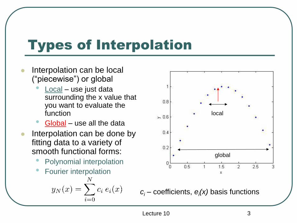
Interpolation can be local (“piecewise”) or global

• Local – use just data surrounding the x value that you want to evaluate the function

• Global – use all the data

Interpolation can be done by fitting data to a variety of smooth functional forms:

• Polynomial interpolation

• Fourier interpolation

local

global

ci – coefficients, ei(x) basis functions

Lecture 10 4

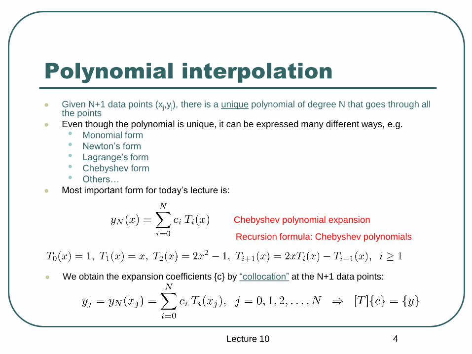
Polynomial interpolation

Given N+1 data points (xj,yj), there is a unique polynomial of degree N that goes through all the points

Even though the polynomial is unique, it can be expressed many different ways, e.g.

• Monomial form

• Newton’s form

• Lagrange’s form

• Chebyshev form

• Others…

Most important form for today’s lecture is:

Chebyshev polynomial expansion

Recursion formula: Chebyshev polynomials

We obtain the expansion coefficients {c} by “collocation” at the N+1 data points:

Lecture 10 5

Local vs. Global Polynomial

Interpolation

Fitting a low-order polynomial to a few points, N · 5, of a data

set that span a point x is a good

way to locally interpolate a

function y(x) near x

Now suppose we want to

evaluate y(x) throughout the

whole domain of x, [-1,1] – i.e.

develop a global interpolant

Can we just interpolate with a

higher-order (degree N >>1)

polynomial through all of the

N+1 points??

Interpolate at x = - 0.3

Lecture 10 6

Global Interpolation Example

Let’s try global interpolation by fitting an N=16 polynomial to a smooth function sampled at 17 equispaced points:

This is a disaster!

The error, while small in the middle, is huge near the boundaries. This is the so-called:

“Runge phenomenon”

Runge

phenomenon

Lecture 10 7

Chebyshev to the rescue

We see that global polynomial interpolation of a large data set of equispaced points can produce disastrous “Runge oscillations” near the boundaries

Remarkably, this problem can be fixed by simply choosing to collocate using unequally spaced data points – the Chebyshev points

These points are the extrema of the polynomial TN(x) over [-1,1]

-1 -0.5 0.5 1

-1

-0.5

0.5

1

Plot of T16(x)

Lecture 10 8

Let’s repeat our example and compare the use of uniformly spaced points versus Chebyshev points for N = 16

Notice that the Chebyshev points are clustered near the boundaries at x = -1, 1

See ChebyInterpL10.m

Problem solved!

We now have a global approximant that is uniformly accurate!

Our example revisited

Lecture 10 9

Errors and Other Intervals

A remarkable feature of global interpolation with Chebyshev polynomials is the rapid rate of convergence. If the function being described is suitably smooth (analytic), the error in the approximant can be shown to decay as fast as

This exponentially fast convergence with the number of data points is referred to as “spectral accuracy” and is highly desirable

To achieve these results, it is very important that the independent (x) variable of your data be scaled to the interval [-1,1] or Chebyshev interpolation will not work!

A simple change of variable will do the trick:

Lecture 10 10

Another Remarkable Fact about

Chebyshev Interpolation

Recall that we obtain the Chebyshev polynomial expansion coefficients {c} by collocation and solving a linear system (polyfit did this for us in our examples)

For large N, this looks expensive, requiring O(N3) flops

However, if we use the Chebyshev points:

Here we have used the property

Thus, {y} and {c} are related by a “Discrete Cosine Transform” (DCT): {y} = [DCT] {c}

The DCT can be performed in O(N log N) operations by a Fast Fourier Transform (FFT) algorithm: much faster! (See Lecture 16)

[DCT]ji

Lecture 10 11

Spline Interpolation

An alternative way to develop a global interpolant for a data set is to use splines

Spline interpolation involves using a different low-order polynomial (<4) in each interval between points (“knots”)

The polynomial coefficients are determined by matching the function values and low-order derivatives (<3) at the knots

Spline interpolants are thus piece-wise continuous functions that are differentiable (smooth) only to low order • Linear spline: y continuous

• Quadratic spline: y,y’ continuous

• Cubic spline: y, y’,y’’ continuous

Linear Spline Fit:

N=16

Notice discontinuous derivative

at “knots”

Lecture 10 12

Constructing a Cubic Spine

With N+1 data points, have N intervals between points. In the ith interval, the approximant is:

We thus have 4N coefficients to determine

These are fixed by the following 4N linear conditions: • The yi(x) must match the data points at each end of each interval: 2N conditions

• The first derivatives must match in adjacent intervals for each interior point (knot): N-1 conditions

• The second derivatives much match in adjacent intervals for each interior point (knot): N-1 conditions

• The second derivatives of the two end points are set to zero (free end conditions): 2 conditions

The result is a “banded” linear system of equations to solve for the 4N coefficients – efficient O(N) algorithms are available (c.f. tridiagonal case)

The banded nature of the spline matrix shows that the spline method is only weakly global – information about the approximant is only tenuously propagated from interval to interval. This is unlike Chebyshev interpolants, where the Ti(xj ) matrix is dense:

Lecture 10 13

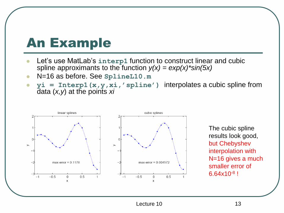
An Example

Let’s use MatLab’s interp1 function to construct linear and cubic spline approximants to the function y(x) = exp(x)*sin(5x)

N=16 as before. See SplineL10.m

yi = Interp1(x,y,xi,’spline’) interpolates a cubic spline from data (x,y) at the points xi

The cubic spline

results look good,

but Chebyshev

interpolation with

N=16 gives a much

smaller error of

6.64x10-8 !

Lecture 10 14

Global Interpolation Summary

Both Spline and Chebyshev interpolation are powerful tools for developing a global approximant to a smooth function sampled at discrete points: • Chebyshev enjoys spectral accuracy (if the function is

analytic) and can be efficiently implemented using FFT methods. The data points have to be sampled at the Chebyshev nodes or roots

• Cubic Spline interpolation converges less rapidly, with errors decaying algebraically as ~N-4, but is easily and efficiently implemented with arbitrary spaced data