Global Games in Macroeconomics

Pau Roldan

⇤

This version: November 17, 2014

Abstract

A large variety of macroeconomic phenomena, including debt crises, speculative attacks, bank

runs, investment crashes and socio-political instability, can be thought to be the outcome of strate-

gic complementarities in payo↵s and actions that foster coordination among economic agents. In

such interpretation, multiple equilibria may emerge. Multiplicity has ambiguous implications from

a positive perspective, and an important strand of the macroeconomic literature has focused on

providing theoretical refinements that can help overcome this issue. In the last two decades, a

stylized and tractable game-theoretic approach building on the global games literature first formu-

lated by Carlsson and van Damme (1993) has been proposed and explored in depth. This paper

reviews the theory of global games, with emphasis on its implications for equilibrium selection, as

well as a few of its recent and most relevant applications to macroeconomics.

⇤New York University, Department of Economics. 19 W 4th Street, O�ce 620. Contact: pau.roldan@nyu.edu.

Contents

1 Introduction 3

2 Theory summary 5

2.1 An introductory example . . . . . . . . . . . . . . . . . . . . . . . . . . . . . . . . . . . 6

2.2 Symmetric binary-action global games . . . . . . . . . . . . . . . . . . . . . . . . . . . . 8

2.2.1 Global games with uniform prior and private values . . . . . . . . . . . . . . . . 8

2.2.2 Global games with generic prior and common values . . . . . . . . . . . . . . . . 10

3 Applications of global games in macroeconomics 11

3.1 Morris and Shin (1998): The baseline game . . . . . . . . . . . . . . . . . . . . . . . . . 12

3.2 The role of market-clearing prices . . . . . . . . . . . . . . . . . . . . . . . . . . . . . . . 16

3.2.1 Angeletos and Werning (2006): Trade in financial markets . . . . . . . . . . . . . 16

3.2.2 Hellwig, Mukherji and Tsyvinski (2006): The role of interest rates . . . . . . . . 20

3.3 The role of equilibrium outcomes as signaling devices . . . . . . . . . . . . . . . . . . . . 28

3.3.1 Angeletos, Hellwig and Pavan (2006): Policy as a signal for the investors . . . . . 28

3.3.2 Goldstein, Ozdenoren and Yuan (2011): Attacks as a signal for the policy-maker 31

3.4 Dynamic models of global games . . . . . . . . . . . . . . . . . . . . . . . . . . . . . . . 34

3.4.1 Morris and Shin (1999): A repeated static global game . . . . . . . . . . . . . . . 35

3.4.2 Angeletos, Hellwig and Pavan (2007): Endogenous dynamics and timing of attacks 37

3.4.3 Steiner (2008): Coordination cycles through the role of participation . . . . . . . 43

4 Discussion 49

4.1 A dynamic partial-equilibrium model of coordination-driven growth . . . . . . . . . . . 50

4.2 A dynamic general-equilibrium model of coordination-driven growth . . . . . . . . . . . 53

5 Concluding remarks 58

2

1 Introduction

An economy is a large macro-structure that is populated by a variety of agents who interact, form

expectations over uncertain future payo↵s and take optimal decisions with respect to their information

sets. There exist many situations in which such interactions may give rise to strategic coordination

motives because individual payo↵s depend not only on an underlying economic fundamental that

shapes the aggregate state of the economy and that the agents might perceive in di↵erent ways, but

also on the actions that other players undertake. In these cases, agents must form beliefs about

what other agents believe, and di↵erent coordination schemes can be sustained and be self-fulfilling in

equilibrium. For example, with the prospect of a devaluation, a great mass of speculators may attack

on a currency if the fundamentals are (or are perceived to be) weak, which in turn would drive the

policy-maker to devaluate for a su�ciently strong attack, thereby confirming the ex-ante expectations

of the individual agents. Importantly, this may occur even when each individual agent is atomistic

and acknowledges that her action alone is insu�cient for such an attack to yield aggregate success.

However, the coordination-driven correlation in actions may push the final outcome to correspond

exactly to the overall prior market expectation.

From this point of view, many macroeconomic phenomena, ranging from debt and currency crises

to investment crashes and political instability, can be understood as the outcome of self-fulfilling

expectations, higher-order beliefs and information processing in an environment of strategic uncertainty

(i.e, uncertainty about the behavior of other agents) and payo↵ complementarities (i.e, actions that

individually deliver a higher payo↵ when also chosen by others). It is therefore natural to model

such scenarios as games in which players interact in coordination and their payo↵s depend on their

own actions, the actions of others and the economic fundamentals. If such fundamentals are common

knowledge, di↵erent agents may tacitly coordinate into choosing the same actions in equilibrium.

There exists a vast body of work in the macroeconomic field in which coordination motives are

responsible for the existence of multiple equilibrium outcomes. In currency and balance-of-payment

crises, this view has historically been split into two major currents. First generation models, starting

with Krugman (1979) and Flood and Garber (1984) and refined by Broner (2008) and others, view

crises as arising from inconsistent policies and the central bank’s inability or unwillingness to sustain

the costs of high interest rates. Second generation models, starting with Obstfeld (1986), view crises

as a coordinated run on the central bank’s reserves of foreign currency. In this latter view, multiple

outcomes can be sustained in equilibrium both because informational di↵erences between investors give

rise to coordination and because asset markets may clear at di↵erent interest rates that are consistent

with an uncovered interest rate parity condition. Chari and Kehoe (2003) show that the investors’

ability to infer other agent’s private information from their actions can account for the unpredictability

3

of crises and for herd-like capital flows. Other models in which debt crises are modeled as coordination

games featuring multiple equilibria are Calvo (1988), Obstfeld (1996) and Cole and Kehoe (2000), to

name a few relevant examples.

Other interpretations include bank runs, asset price crashes, fluctuations in search activity and

episodes of revolution and socio-political distress. For bank runs, Diamond and Dybvig (1983) show

that even stable banks may be vulnerable to self-fulfilling panics if there is a systemic mismatch of

long-maturity assets and short-maturity liabilities. In the spirit of the global games selection mecha-

nism described below, Goldstein and Pauzner (2005) resolve this equilibrium indeterminacy by adding

idiosyncratic noise into an otherwise identical economy, which allows the analysis to provide unam-

biguous statements regarding the probability of runs and the welfare of banks. Within the literature on

asset market crashes, Barlevy and Veronesi (2003) show that uninformed stock market investors who

panic may cause asset prices to plummet and precipitate financial crises because they react too strongly

against fundamentally-driven declining prices. This interpretation again emphasizes the informational

friction as being at the core of the main amplification force behind the large impact of seemingly small

shocks. For applications to search, Diamond (1982) showed that multiplicity of equilibria can arise

from a matching problem with trading frictions in which recessions, as henceforth viewed by Keyne-

sians, are associated with “coordination failures”. Based on this result, Steiner (2008) provides a brief

but enlightening example of fluctuations in search activity within the framework that we will analyze

in section 3.4.3. Finally, for socio-political crises, Edmond (2013), inspired by Atkeson’s (2000) com-

ments on Morris and Shin (1998), presents a model of revolution against a political regime in which

the information manipulation by autocratic authorities may ensure their survival.

Although diverse in style, the models briefly surveyed above all share the idea that information

heterogeneities may themselves be at the core of financial crises. While this view is appealing, two

rather technical concerns immediately arise from it. First, since coordination requires rationality

in the choice of one’s actions as a best response to those of others, it also demands the individual

forecast of others’ actions and, in turn, of others’ forecasts about such actions. Since others’ beliefs

become individual states, one may need to condition on the entire infinite hierarchy of higher-order

beliefs in order to fully describe the equilibrium set of the economy. This dimensionality problem can

become intractable if not adequately dealt with1. Second, when economic fundamentals are common

knowledge, coordination may give rise to multiplicity. This is an issue for drawing both determinate

economic predictions and unambiguous policy implications.

Global games o↵er a tractable and stylized solution to both these concerns. A global game is

said to be a game of incomplete information within an environment of strategic uncertainty in which

1This is a well-understood problem that goes back to the classic rational expectations revolution literature in macroe-conomics, including Muth (1961), Lucas (1975), Townsend (1983), and Sargent (1991), among others.

4

players receive private signals on unknown economic fundamentals. By introducing private noise, the

coordination motive is dampened: if the quality of the private signal is su�ciently high (as measured

by the precision of its noise), agents will place enough weight on information others do not share and

multiplicity will not to arise in equilibrium. If they expect other agents to behave in a similar fashion,

this behavior can aggregate up enough for the model to select a unique outcome. In the words of

Chamley (2003), “the problem of multiple equilibria disappears because a contagion process from the

agents with extreme beliefs leads all other agents either to action or to inaction”. In short, private

information eliminates the multiplicity e↵ects of common knowledge if the former is su�ciently precise:

uniqueness obtains as a perturbation away from perfect information. Moreover, under regularity

conditions on payo↵s, the model can be solved by iterated deletion of dominated strategies and reduced

into an analysis by threshold strategies, which enable the agents to make use of a more tractable belief

inference without loss of generality and reduces the dimensionality of the problem immensely as higher-

order expectations drop out of the relevant state of the economy. These insights were first shown by

Carlsson and van Damme (1993) and later on applied in macroeconomics, most notably by Morris and

Shin (1998).

In this paper, I present the basic theory of global coordination games and review a few applica-

tions in macroeconomics. To fix ideas, Section 2 o↵ers an introduction to simple global games, as

presented by Carlsson and van Damme (1993) and further developed by Morris and Shin (2003). This

section presents key technical results that rely on the payo↵ structure of the game and are key for

the equilibrium selection mechanisms provided later on to be e↵ective. In Section 3, I present several

recent applications of the literature to common macroeconomic problems. I start with Morris and Shin

(1998), who first introduced a uniqueness result in a model of currency crises. The remainder of the

section is devoted to studying di↵erent extensions of the baseline model in relevant dimensions under

which the uniqueness result breaks down. The intuition is simple: introducing public information,

either exogenously or endogenously through information aggregation in market prices, signaling in

public policy or periodical revelation of information in dynamic settings, provides a common source of

knowledge that allows agents to coordinate in their actions. In this strand of literature, I will review

a few of what I consider to be the most insightful papers. Section 4 includes a discussion and outlines

a potential line of further research on the topic. Section 5 concludes.

2 Theory summary

This section reviews the general theory behind the global game approach to economic problems that

exhibit complementarities in actions, payo↵s and, possibly, information. In the general framework,

the fundamentals of the economy are assumed to be summarized by a single state variable ✓ 2 R

5

which enters the payo↵ function of the decision maker. If this state is common knowledge, agents can

exploit their shared information and coordinate in equilibrium to give rise to a multiplicity of outcomes.

However, we additionally suppose that each agent observes a di↵erent signal that is private information

to that agent. Assuming that the noise technology is common knowledge, but the fundamental state

✓ is not, agents must form beliefs about the fundamentals, about other players’ beliefs about the

fundamentals, about other players’ beliefs about such beliefs, and so on. We next analyze how this

can be made tractable.

2.1 An introductory example

Take the following example from Carlsson and van Damme (1993). There are two players, indexed

i = 1, 2, unilaterally choosing an action a

i

2 {0, 1} in a one-shot simultaneous game. For example,

consider ai

= 1 to be investment, and a

i

= 0 no investment. Their payo↵s are summarized in Table 1.

The fundamental ✓ 2 R is drawn by nature before the game starts.

a2 = 1 a2 = 0

a1 = 1 ✓,✓ ✓ � 1,0a1 = 0 0,✓ � 1 0,0

Table 1: Payo↵ matrix for the investment game example.

Suppose first that ✓ is common knowledge among the players. The game can be solved in three

cases. If ✓ > 1, then each player has a dominant strategy to invest and (1, 1) is the unique Nash

equilibrium in pure strategies. If ✓ < 0, each player has a dominant strategy not to invest and (0, 0)

is the unique Nash equilibrium in pure strategies. Finally, for any ✓ 2 (0, 1), both agents investing

and both not investing can be sustained as pure Nash equilibria. Overall, the game exhibits multiple

equilibria.

Now, assume that ✓ is not common knowledge and there is incomplete information. Nature draws

✓ from a uniform over the real line. This can be thought of being a so-called di↵use (or uninformative)

common prior belief about ✓. Additionally, each agent i receives a signal xi

that is private information,

with

x

i

= ✓ + "

i

where "i

⇠ N (0, 1/�) and � � 0 is the so-called precision of the private signal. Endowed with this

information, agent i’s posterior belief about ✓ is

6

✓|xi

⇠ N (xi

, 1/�)

Note that, since the information technology is common knowledge, this agent believes his opponent’s

signal to be distributed according to x�i

|xi

⇠ N (0, 2/�).

A strategy for player i is a map x

i

7! {0, 1} which we call s. The solution can in principle involve

the infinite inference of beliefs between the two agents. However, a much simpler solution procedure

based on iterative deletion of dominated strategies turns out to be of use here. We will shortly analyze

conditions under which such solutions can be applied in more general settings.

Conjecture that the solution is in so-called threshold (or monotone) strategies. This is, suppose

that there exists a cut-o↵ point x⇤ 2 R such that we can write the optimal strategy by

s(xi

) = 1[xi

>x

⇤]

for either i, where 1[·] is an indicator function. This means that the agent will choose not to invest

if his signal realization conveys information about the fundamental having a bad enough realization,

given what the other player’s beliefs are and what her beliefs about the beliefs are, as represented by

a realization of the signal that is below the threshold value. This strategy is thus a switching strategy

around x

⇤, and is monotone in the sense that there is only one such switching point2.

Under this strategy, the posterior probability assigned by i to her opponent choosing to invest is

P[x�i

> x

⇤] = 1� � r

�

2(x⇤ � x)

!

where �(·) henceforth denotes the c.d.f. of the standard normal distribution. For example, if the

player has observed a signal that is equal to the cutting point of the opponent, she will always assign

probability 1/2 to her opponent choosing to invest.

The conjecture will be confirmed if we can find the value x⇤ that can sustain the proposed strategy

profile as an equilibrium outcome. To do this, we will follow an iterated deletion of strictly dominated

strategies procedure. Morris and Shin (2003) provide the following insight: let b(x⇤) be the unique

value of x solving the equation

x� � r

�

2(x⇤ � x)

!= 0

This means that if the player’s opponent is following a switching strategy with cuto↵ x

⇤, the player’s

best response is to follow a switching strategy with cuto↵ b(x⇤). It can be argued by induction that if

2The agent is indi↵erent at the switching point, so we should rigorously call this an essentially unique solution.Because this is common in all the models that we will study here, we will henceforth ignore this nomenclature.

7

a strategy s survives n 2 N rounds of iterated deletion of strictly dominated strategies, then we can

write

s

i

(xi

) =

8><

>:

1 if xi

> b

n�1(1)

0 if xi

< b

n�1(0)

If the player knew that the opponent would choose action a�i

= 0 if she had observed a signal less

than b

n�1(1), then her own best response would always be to choose action a

i

= 0 if her signal was

less than b(bn�1(1)) ⌘ b

n(1). Moreover, b(·) can be shown to be increasing and to have a unique fixed

point at 1/2, so

limn!+1

b

n(0) =1

2= lim

n!+1b

n(1)

and therefore the equilibrium is in monotone threshold strategies with x

⇤ = 12 .

2.2 Symmetric binary-action global games

The previous example illustrated two key results. First, in simultaneous one-shot two-by-two global

games in which the prior is di↵use, introducing idiosyncratic noise in the information structure reduces

the set of equilibria to a singleton. Second, the analytical convenience of solving for switching strategies

with no loss of generality allows the agents to form beliefs that are based on a single layer of rationality,

as opposed to an infinite hierarchy. Morris and Shin (2003) show that this insight extends to similar

games with more players (for instance a continuum of them), non-binary choices and asymmetric

payo↵s. Moreover, when the common prior is not di↵use and there is meaningful public information

that partially restores common knowledge, uniqueness can still arise under parametric conditions on

the relative signal precisions.

In the present paper I will only review models that make use of symmetric-payo↵ binary games and

a continuum of players3. Therefore, for later reference, the remainder of this section provides general

results for such type of games.

2.2.1 Global games with uniform prior and private values

We first consider the case of a uniform common prior on the state and each player’s signal being a

su�cient statistic for how much they care about the state (private information).

3Having a continuum of players allows us to invoke the law of large numbers in order to approximate aggregate choicesas expected outcomes. It also means that each agent is atomistic, and thus cannot unilaterally influence the aggregateoutcome and, therefore, the action of others (see Corsetti et al. (2004) for a study on large players). Moreover, in allour examples, individual actions will not be observable by others, except for the aggregate action. This means thato↵-equilibrium beliefs will not have to be specified.

8

There is a continuum of players of unit mass. Each chooses an action a 2 {0, 1} and has utility

u : {0, 1}⇥ [0, 1]⇥R ! R, where u(a,A, x) is the payo↵ of the individual when taking action a, when

A is the proportion of individuals that take action a = 1 and when the private signal is x. Define

marginal utility ⇡ : [0, 1]⇥ R ! R by

⇡(A, x) ⌘ u(1, A, x)� u(0, A, x)

Before the game starts, a state ✓ 2 R is drawn from an improper uniform density on the real line,

and individual i’s private signal is

x

i

= ✓ +"

ip�

where � > 0 denotes precision and "i

has a continuous density f(·) with support R. It can be shown

that an individual with signal xi

puts (posterior) densityp�f(

p�(x

i

� ✓)) on state the realization of

a particular state ✓.

We assume that the following properties hold:

• A1. Action monotonicity: ⇡(A, ✓) is nondecreasing in A.

• A2. State monotonicity: ⇡(A, ✓) is nondecreasing in ✓.

• A3. Strict Laplacian state monotonicity: There exists a unique ✓⇤ that solves

Z 1

0⇡(A, ✓

⇤)dA = 0 (1)

• A4. Limit dominance: There exist ✓ 2 R and ✓ 2 R such that (i) ⇡(A, x) < 0 for all A 2 [0, 1]

and x ✓; and (ii) ⇡(A, x) > 0 for all A 2 [0, 1] and x � ✓.

• A5. Continuity: The functionR 10 g(A)⇡(A, x)dA is continuous with respect to signal x and

density g(·).

Assumption A1, which states that each player’s utility function is supermodular in the action profile,

implies that there exist strategic complementarities in the game: the individual receives more payo↵

by choosing a = 1 when a larger size of the population is choosing a = 1 as well. Assumption A2 states

that each player’s utility function is supermodular in her own action and the state, too. Assumption A3

is a single-crossing property ensuring that there is at most one crossing in the optimal policy function

for a player with Laplacian beliefs4. Assumption A4 implies that action 0 (1) is a dominant strategy

for su�ciently low (high) signals. Finally, assumption A5 imposes a weak continuity condition.

4According to the definition provided by Morris and Shin (2003), an agent has so-called Laplacian beliefs if she appliesa uniform prior to unknown events from the “principle of insu�cient reason”. That is, each agent hypothesizes that

9

Refer to the game described above and endowed with assumptions A1 to A5 by G

⇤(�). Define

a strategy for a player in the incomplete information game G

⇤(�) as a function s : R ! {0, 1},

where s(x) 2 {0, 1} is the action chosen if a player observes signal x5. Then, we obtain the following

generalization of the result obtained in Section 2.1:

Proposition 1 Let ✓⇤ be defined as in equation (1). Then, the unique perfect Bayesian Nash equilib-

rium (PBE) strategy that survives iterated deletion of strictly dominated strategies in G

⇤(�) is

s(x) =

8><

>:

0 for x ✓

⇤

1 for x � ✓

⇤

Proof: In Morris and Shin (2003), page 66. ⌅

This result shows that one can focus on symmetric monotone PBE in this framework without any

loss of generality. In particular, assumptions A1 and A2 can be shown to be su�cient for equilibria

to be monotonic with respect to agent types (the latter here symbolized by the switching threshold).

Within this class of monotone equilibria, A3 then ensures symmetry and uniqueness. Although there

are ways of relaxing these assumptions (see Morris and Shin (2003), section 2.2.3), assumptions A1,

A2 and A3 are key for the uniqueness results in most static binary global games set-ups.

2.2.2 Global games with generic prior and common values

As it turns out, the insights behind Proposition 1 extend to games with an even more generic

structure. Suppose now that ✓ is instead drawn from a continuously di↵erentiable strictly positive

density p(·) on the real line. Moreover, a player’s utility depends on the realized state ✓, not his

signal x on ✓. Thus, u(a,A, ✓) is the payo↵ if the player chooses action a 2 {0, 1}, a proportion

A 2 [0, 1] of individuals choose action a = 1 and the realized state is ✓. Let, as before, ⇡(A, ✓) ⌘

u(1, A, ✓)� u(0, A, ✓).

We need the following additional assumptions:

• A4*. Uniform limit dominance: There exists ✓ 2 R, ✓ 2 R, and " 2 R++, such that (i)

⇡(A, x) �" for all A 2 [0, 1] and x ✓; and (ii) ⇡(A, x) > " for all A 2 [0, 1] and x � ✓.

• A6. Integrability: The functionR +1�1 zf(z)dz is well-defined.

the proportion of other players who will opt for each action is a uniform random variable over the unit interval. As aconsequence, agents choose an action that is a best response to a uniform belief over the proportion of her opponentschoosing each action. The agents in all the global games that I will present here are, in this sense, Laplacian players.

5Note all i subscripts have been dropped, for each individual can now be indexed by the signal she receives.

10

Assumption A4*, which will replace A4, says that the payo↵ gain to choosing action 0 (1) is

uniformly positive for su�ciently low (high) values of ✓. Assumption A6 ensures that a well-defined

distribution of the noise exists.

Let G(�) denote the incomplete information game with properties A1, A2, A3, A4*, A5 and A6.

The following extension of Proposition 1 holds:

Proposition 2 Let ✓⇤ be defined as in equation (1). For any � > 0, there exists � > 0 such that for

all � �, if strategy s survives iterated deletion of strictly dominated strategies in the game G(�),

then

s(x) =

8><

>:

0 for x ✓

⇤ � �

1 for x � ✓

⇤ + �

Proof: In Morris and Shin (2003), page 68. ⌅

This result therefore says that the uniform prior, private-values game G

⇤(�) is the limit of the

general prior, common-values game G(�) as � becomes arbitrarily large. That is, the posterior beliefs

when private noise is insignificant are almost the same as under a uniform prior.

3 Applications of global games in macroeconomics

The previous section has presented a few critical results for generic games of incomplete information.

This section puts those results into use and provides a review of the literature of global games in

macroeconomics. Many di↵erent interpretations can be provided of the global games approach. In

currency crises, Morris and Shin (1998, 1999), Chamley (2003), Corsetti, Dasgupta, Morris and Shin

(2004), Hellwig, Mukherji and Tsyvinski (2006), Angeletos, Hellwig and Pavan (2006), and Goldstein,

Ozdenoren and Yuan (2011) are some key references. Rochet and Vives (2004) and Corsetti, Guimaraes

and Roubini (2006) in debt crises and Goldstein and Pauzner (2005) in bank runs are other classical

applications. Morris and Shin (2004) apply the insights of Morris and Shin (1998) to a model of debt

pricing. Alternative possible interpretations include liquidity crises, investment crashes, adoption of

new technologies and socio-political unrest.

I start with a brief description of Morris and Shin (1998), a seminal paper showing equilibrium

uniqueness results similar to the ones discussed above within a global game of regime change. I provide

a slightly simplified version of the paper in a way that the model can, but need not, be interpreted

as a second-generation model of currency crises. Moreover, the notation is adapted in a way to

11

accommodate almost all the models that will follow, and to which the basic Morris and Shin game will

serve as a baseline.

3.1 Morris and Shin (1998): The baseline game

Consider a single-shot game in an economy populated by a measure-one continuum of agents,

i 2 [0, 1], and a policy-maker (or central bank). Each agent chooses an action a

i

2 {0, 1} which we

interpret as attacking a status quo (a = 1) or not attacking it (a = 0). There is an opportunity cost

c 2 (0, 1) of attacking. The status quo is abandoned (and therefore the attack is successful) if enough

agents individually choose to attack it relative to the level fundamental, ✓ 2 R, which represents

the strength of the status quo. In particular, there is regime change if, and only if, A > ✓, where

A ⌘R 10 a

j

dj is size of the attack. The regime outcome can thus be expressed as

R(✓) ⌘ 1[A>✓]

and the ex-post individual payo↵ can compactly be given by

U(ai

, A, ✓) = a

i

(R(✓)� c)

This payo↵ says that no attacking individually earns a payo↵ of zero. Attacking earns a payo↵ of

1� c > 0 if the status quo is abandoned, and �c < 0 otherwise.

This framework is general enough to be interpreted in di↵erent ways. In Morris and Shin’s original

description, the status quo is a fixed exchange rate regime, and action a = 1 is interpreted as attacking

the peg by exchanging domestic for foreign currency in the central bank. The fundamental ✓ can be

viewed to proxy for the policy-maker’s cost of defending the fixed regime, whereas A stands for the

amount of reserves of foreign currency that are withdrawn by the population of investors6.

Just as in our first simple example, if the fundamental ✓ were common knowledge, the model would

exhibit multiple equilibria. Again, the solution is almost trivial for ✓ < 0 (where nobody attacking is a

pure Nash equilibrium) and ✓ > 1 (where all attacking is a pure Nash equilibrium). Otherwise, there

is a nonempty set [✓, ✓] ✓ [0, 1] such that all attack if ✓ ✓ and nobody attacks if ✓ � ✓. If ✓ 2 (✓, ✓),

both attack and no attack can be sustained in equilibrium.

Suppose, however, that the fundamental ✓ is not common knowledge among the players. We assume

6More particularly, in their paper, there is a currency pegged to an exchange rate e⇤ which, if the policy-makerdecides to abandon, will float to a rate ⇣(✓) e⇤, where ⇣(·) is an increasing and continuous function. A continuumof speculators with unit measure decides whether or not to short-sell the currency, and the transaction cost of suchan operation is c. The policy-maker defends the currency if the measure of speculators attacking is lower than somelevel k(✓), where k(·) is continuous and increasing. The instantaneous payo↵ of attacking is zero, while attacking earnsa payo↵ of e⇤ � ⇣(✓) � c if k(✓) < A

t

, and �c otherwise. In the set-up we have described, therefore, we have simplyassumed that k(✓) = ✓ and e⇤ � ⇣(✓) = 1, 8✓ 2 R, in order for the model to allow a much more general interpretation.None of the key results depend on these simplifications.

12

that ✓ is observed with noise through the following information structure. At the beginning of time,

nature draws

✓ ⇠ N (z, 1/↵)

or, equivalently, ✓ = z + " with " ⇠ N (0, 1/↵) and (z,↵) common knowledge, and each agent i

receives a private signal

x

i

= ✓ + ⇠

i

where ⇠i

⇠ N (0, 1/�). Once again, we can then index each individual by the signal this individual

receives. Define again the marginal payo↵ as

⇡(A, ✓) ⌘ U(1, A, ✓)� U(0, A, ✓)

Note that assumptions A1, A2 and A3 hold, and therefore the equilibrium analysis from Section 2

can be used. In particular, we can solve for the monotone Bayesian Nash equilibrium by looking for

threshold policies without loss of generality. An informal argument is as follows: note that the c.d.f.

of the agent’s posterior about ✓ is decreasing in x, meaning that an agent believes a high signal to

convey information about a strong fundamental. Moreover, for x < x, where x solves P[✓ 0|x] = c,

attacking is strictly dominant, whereas for x > x, where x solves P[✓ � 1|x] = 1 � c, not attacking

is strictly dominant. Using the monotonicity of beliefs, there must exist a switching point x⇤ 2 [x, x]

below which an individual would choose to attack, and above which the individual would refrain from

doing so.

Therefore, conjecture once more that there is a level x⇤ 2 R such that we can write the optimal

individual strategy as s(x) = 1[x>x

⇤]. Under this conjecture, the aggregate size of the attack is

A(✓) = P[x x

⇤|✓] = �⇣p

�(x⇤ � ✓)⌘

and thus the status quo is abandoned if and only if ✓ ✓

⇤, where ✓⇤ solves ✓⇤ = A(✓⇤), that is

✓

⇤ = �⇣p

�(x⇤ � ✓

⇤)⌘

(2)

On the other hand, x⇤ is the signal that makes the marginal investor indi↵erent between attacking

and not attacking, or P[✓ ✓

⇤|x⇤] = c, that is

1� �✓p

� + ↵

✓�x

⇤ + ↵z

� + ↵

� ✓

⇤◆◆

= c (3)

13

Equations (2) and (3) jointly determine the solution for thresholds (✓⇤, x⇤), confirm the conjecture

and characterize the equilibrium.

Since the common prior is not di↵use, agents can coordinate on the information they share (whose

precision is given by ↵), and multiple equilibria may arise if the quality of private knowledge is not

high enough. Conversely, a su�ciently precise private signal ensures uniqueness. The next result

summarizes this result:

Proposition 3 The equilibrium is unique if and only if private noise is small relative to public noise,

so that

� � ↵

2

2⇡(4)

and is in monotone strategies.

Proof: In Angeletos, Hellwig and Pavan (2007), page 744. ⌅

In other words, provided that the parametric condition (4) holds, Proposition 3 tells us that unique-

ness holds as perturbation away from common knowledge. Note that a tiny amount of noise with respect

to the perfect information benchmark (the limit of which is � = +1) is su�cient to break multiplic-

ity insofar as condition (4) continues to hold. This is because private information anchors individual

behavior and limits the ability to forecast one another’s actions, and thus non-fundamental volatility

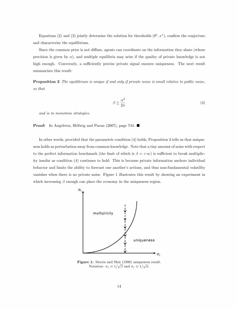
vanishes when there is no private noise. Figure 1 illustrates this result by showing an experiment in

which increasing � enough can place the economy in the uniqueness region.

Figure 1: Morris and Shin (1998) uniqueness result.

Notation: �x

⌘ 1/p� and �

z

⌘ 1/p↵.

14

What is more, for given ↵, when the noise in private information is small, then ✓

⇤ converges to

✓1 ⌘ 1 � c, and whenever ✓ is in the neighborhood of ✓1, a small variation in ✓ can trigger a large

and discrete variation in the size of the attack and in the regime outcome:

Proposition 4 For given ↵, as � ! +1, the equilibrium size of the attack is described by:

A(✓) �!

8><

>:

1 if ✓ < ✓1

0 otherwise

Proof: In Angeletos and Werning (2006), page 1732. ⌅

Proposition 4 states that there is a large and discontinuous nonfundamental volatility embedded in

the type of crises that a global game can generate: when agents are perfectly privately informed, they

are able to globally coordinate on the regime outcome, and a low enough fundamental may trigger an

economy-wide attack and a subsequently large devaluation.

The simple version of the model just outlined has the advantage of providing clear and testable

predictions. Rather than merely o↵ering a mechanism with which to select an equilibrium outcome,

in the same spirit as a sunspot variable would do, the global game changes the information structure

of the players and, by introducing information that cannot be shared between investors, eliminates all

strategic motives that may give rise to multiple coordinated outcomes.

Although unambiguous in its prediction, the model’s main results are however not robust to altering

the information structure. Indeed, introducing additional motives for coordination can show how

unstable uniqueness becomes.

A first straightforward way is to introduce exogenous public signals that are precise enough relative

to the private signal. This has been studied, for example, by Hellwig (2002) and Hellwig and Veldkamp

(2008), among others. Both these papers show that in settings in which there are complementarities

in actions, the agents’ optimal choices of information acquisition exhibit complementarities as well.

A second well-explored mechanism through which equilibrium uniqueness may break down is the

introduction of public information through endogenous equilibrium outcomes. The remainder of this

section explores this second channel. First, I will review the role of information aggregation provided

by equilibrium prices, be it asset prices (Angeletos and Werning (2006)) or interest rates (Hellwig,

Mukherji and Tsyvinski (2006)). Second, I will move on to studying public information revealed by

government policies, which act as signaling devices that may a↵ect the outcomes of the Morris and Shin

game in critical ways. The papers I will describe in this strand of literature are Angeletos, Hellwig and

Pavan (2006) and Goldstein, Ozdenoren and Yuan (2011). Finally, I will focus on public information

15

introduced endogenously through the periodical revelation embedded within past outcomes and the

role of coordination cycles within dynamic global games settings. In this literature, I will review three

papers: Morris and Shin (1999), Angeletos, Hellwig and Pavan (2007) and Steiner (2008).

3.2 The role of market-clearing prices

If a Morris and Shin (1998) game is augmented to introduce equilibrium prices that must clear the

markets, the observation of such prices prior to the coordination game may allow the agents to make

inference about the state of the economy. If this information is shared by everyone, coordination may

be reinforced, actions may feedback back and forth between market activities and speculative episodes,

and multiplicity may once again arise. Indeed, if market activities depend on the information that

is privately owned by agents, there may exist interesting interactions between public knowledge and

private precision. Angeletos and Werning (2006) provide one such example when there is the possibility

of trade.

3.2.1 Angeletos and Werning (2006): Trade in financial markets

Consider the Morris and Shin game of Section 3.1 and suppose it is augmented in the following

way. Prior to the speculative attack stage, now a second stage within the game, there exists a first

stage in which each agent i 2 [0, 1] can trade over a risky asset with dividend f(✓) at a price p. Agent i

must choose the amount k of her wealth w to allocate to the risky asset in order to maximize a CARA

objective:

v(w) = �e

��w

where � > 0 is the coe�cient of risk aversion and w is total individual wealth, given by

w = w0 � pk + f(✓)k

where w0 � 0 is an initial level of wealth. In order to prevent prices from being perfectly revealing,

the asset supply is stochastic7 and given by

K

s(") ="p�

where " ⇠ N (0, 1) is the supply noise and � > 0 is a commonly observed precision. Once trade has

ended, prices are observed and individuals play a Morris and Shin (1998) game in the second stage.

7Otherwise, the Grossman and Stiglitz (1980) paradox would emerge: if all information were reflected in the price(that is, if markets were informationally e�cient), no trader would have the incentive to spend resources in order togather information and trade on it, which would contradict that all information can be included in the price.

16

This stage is identical to the model described in Section 3.1, and therefore all details are suppressed

here.

The following describes an equilibrium of this economy:

Definition 1 An equilibrium is a price function P (✓, "), individual strategies for investment and at-

tacking, k(x, p) and a(x, p), and their corresponding aggregates, K(✓, p) and A(✓, p), such that:

k(x, p) 2 argmaxk2R

E[v(w0 + (f(✓)� p)k)|x, p]

K(✓, p) = E[k(x, p)|✓, p]

K(✓, P (✓, ")) = K

s(")

a(x, p) 2 arg maxa2{0,1}

E[U(a,A(✓, p), ✓)|x, p]

A(✓, p) = E[a(x, p)|✓, p]

This definition says that the first-stage optimal portfolio of the individual maximizes ex-ante ex-

pected utility given the budget constraint, where the expectation is taken with respect to the indi-

vidual’s information set (first equation); the aggregate demand of the asset at any price is the sum

of all the individual demands (second equation); asset prices P (✓, ") clear the asset market given the

asset supply (third equation); the second-stage choice a 2 {0, 1} of whether or not to attack maximizes

expected utility of attacking (fourth equation); and the aggregate size of the attack is the sum of all

the attacks (fifth equation). As before, we define the equilibrium regime outcome as

R(✓, ") ⌘ 1[A(✓,P (✓,"))>✓]

For simplicity, suppose that dividends are given by f(✓) = ✓. Solving for the equilibrium, we can

guess a linear price function that is not perfectly revealing. By Bayes’ rule, the price is a normally

distributed public signal with precision �p

, and the posterior fundamental is

✓|x, p ⇠ N✓�x+ �

p

p

� + �

p

,

1

� + �

p

◆

Since agents have CARA utility, their individual asset demand is the ratio of the mean excess

posterior return on volatility of posterior return (a Sharpe ratio):

k(x, p) =�(x� p)

�

Clearing the asset market, the equilibrium price can be found to be:

17

P (✓, ") = ✓ � "p�

p

where

�

p

⌘ �

2�

�

2

In sum, the price is a signal that the agents use in the second stage during the speculative attack

game. Note that this signal is endogenous and public, as it emerges from equilibrium trade. Impor-

tantly, public information now improves with private information, as �p

is an increasing function in �.

Intuitively, when agents are better privately informed about the fundamental, they are better informed

about the dividend that the asset will pay out, which makes trade become less risky and prices to be

more informative. This is because when private signals are more precise, asset demands are more sen-

sitive and equilibrium prices react more to fundamental than to non-fundamental variables, conveying

more precise information.

Crucially, whereas in the Morris and Shin (1998) game of Section 3.1 one could increase the precision

of private information and enter the uniqueness region with a fixed quality of public information (recall

Figure 1), this is no longer possible as better private information entails now better public information.

Furthermore, if private precision increases at a fast enough rate, the economy might never leave the

multiplicity region, which may therefore survive even as a negligible perturbation away from perfect

information. This last case is illustrated by Figure 2.

Figure 2: Angeletos and Werning (2006) multiplicity result.

Notation: �x

⌘ 1/p�, �

z

⌘ 1/p↵ and �

p

⌘ 1/p

�p

.

The next proposition provides the formal statement: in contrast to Proposition 3, uniqueness holds

for a su�ciently small private information precision, conditional on public information precision being

18

small too.

Proposition 5 There are multiple equilibria if either � or � (or both) are large enough. In particular,

if the following parametric condition holds:

��

p� > �

2p2⇡

Proof: In Angeletos and Werning (2006), page 1732. ⌅

Therefore, multiplicity is ensured when better private information improves public information

at a rate that is fast enough. In particular, for the argument to of through, the endogenous public

noise must fall at a rate faster than does the square root of the exogenous public noise. In this case,

uniqueness can no longer be viewed as a small perturbation away from perfect information, and crises

may arise as episodes of non-fundamental volatility (e.g., sunspots that select the equilibrium outcome)

in which informative variables are being closely monitored8.

A second result refers to the perfect information limit of this economy:

Proposition 6 As either source of noise vanishes (� ! +1 for given �, or � ! +1 for given �),

there exists a passive equilibrium in which R(✓, ") ! 0 for any ✓ 2 (✓, ✓), as well as an aggressive

equilibrium in which R(✓, ") ! 1, for any ✓ 2 (✓, ✓).

Proof: In Angeletos and Werning (2006), page 1732. ⌅

Therefore, in contrast to the statement of Proposition 4, it is no longer true that there is a

unique discontinuity in the regime outcome in the perfect information limit, as both extreme common-

knowledge outcomes can be recovered as either source of noise vanishes: the regime can be either

abandoned or maintained regardless of the fundamental ✓. In this sense, non-fundamental volatility

is non-vanishing even when either source of noise is negligibly small, and multiplicity emerges in the

limit. This result is in sharp contrast to the Morris and Shin benchmark of Section 3.1, and turns

out to be robust to making the dividend endogenous (a function of the aggregate state A) and to

introducing the possibility for agents to observe the actions of each other (see sections III and IV in

Angeletos and Werning (2006) for details).

In sum, Angeletos and Werning (2006) show that the uniqueness result highlighted in Section

3.1 is fragile to adapting the information structure to a market game that, if played prior to the

coordination stage, delivers outcomes that foster otherwise absent coordination within the strategic

8Yet another interpretation comes from using the definition of �p

and restating the parametric condition as�

pp�

>p2⇡.

Thus, multiplicity requires the precision of the price signal to be high enough.

19

uncertainty framework. This channel emphasizes the feedback e↵ects that private information exhibits

in relation to the public information that is inferred from first-stage equilibrium outcomes, and is

shown to be robust enough to survive in the perfect information limit. However, as we show next,

multiplicity need not stem from information complementarities. We next examine an example in which

multiplicity will emerge from market outcomes directly as opposed to indirectly through the e↵ect of

such outcomes on the information set of the agents.

3.2.2 Hellwig, Mukherji and Tsyvinski (2006): The role of interest rates

In the speculative attack interpretation of both Morris and Shin (1998) and Angeletos and Werning

(2006), a successful attack is viewed as a coordinated run on the central bank’s foreign reserves when

interest rates are exogenously determined and the policy-maker’s decision is mechanically driven by

the strength with which the status quo (a peg) can be maintained. Within a similar game in which

investors are heterogeneous in their information endowment, Hellwig, Mukherji and Tsyvinski (2006)

emphasize the role of market-clearing interest rates and explore the multiplicity channel that is origi-

nated in deeper market interactions than those studied by Morris and Shin. By focusing on the role of

equilibrium prices, not only they are capable of examining the feedback interactions between endoge-

nous public information and exogenous private information, as in Angeletos and Werning, but also they

can disentangle these e↵ects from those that are purely due to the market-clearing conditions in the

domestic bond market, and which manifest themselves in the form of non-monotonic demand schedules

and, therefore, multiple market-clearing prices even in the absence of informational incompleteness9.

Consider the following economy. There is a mass-one continuum of agents i 2 [0, 1] called traders.

Each trader is endowed with one unit of domestic currency and must choose only one of two possible

actions: buy the domestic bond, which returns a safe market-determined interest rate r > 0, or

exchange the endowment for foreign currency in the central bank (CB), which earns a net return of

one in case of devaluation, and nothing if the CB decides to maintain the peg. The investment returns

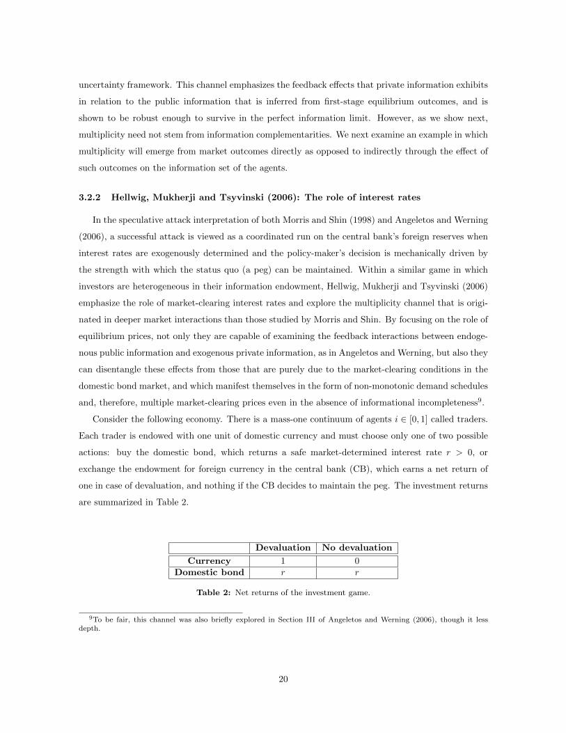
are summarized in Table 2.

Devaluation No devaluation

Currency 1 0Domestic bond r r

Table 2: Net returns of the investment game.

9To be fair, this channel was also briefly explored in Section III of Angeletos and Werning (2006), though it lessdepth.

20

The CB acts as in the standard Morris and Shin game in the sense that it mechanically compares

the costs of devaluations against the strength of the status quo. Whereas this cost was in our original

example equal to the size of the attack A (interpreted as the loss of foreign reserves, or total amount

of foreign currency withdrawn by traders), here it may potentially also depend on interest rates, r.

Denoting the cost of maintaining the status quo by C(r, A), the CB will choose to devaluate if and

only if

✓ C(r, A)

where C(·) is increasing in both arguments. In this way, the model will be able to analyze scenarios

in which devaluations are triggered by high interest rates, as in Obstfeld (1996), as well as cases in

which devaluations are the result of unsustainable reserve losses after coordinated runs on CB deposits,

as in Morris and Shin (1998) and second generation models of currency crises in the spirit of Obstfeld

(1986).

The game unfolds in three stages. In the first stage, nature draws the fundamental from a uniform

with support in the real line (an improper common prior), such that a priori any realization of ✓ 2 R

is deemed equally likely. In addition, each trader i receives an unbiased private signal:

x

i

= ✓ + ⇠

i

where ⇠i

⇠ N (0, 1/�). In the second stage, the domestic bond market and the CB open, and

traders submit contingent bid schedules

a(xi

, r) 2 [0, 1]

d(xi

, r) = 1� a(xi

, r)

on foreign currency holding and domestic bond holdings, respectively. The supply of bonds is

exogenously given by10

S(s, r) = �(s� ���1(r))

where �(·) is the c.d.f. of a standard normal, � � 0 controls the price elasticity of the bond supply

(with � = 0 meaning that the supply is inelastic), and s is a supply shock

10The functional form of S(s, r) is inessential but tractable. What is essential is that S1(·) > 0 and S2(·) � 0.

21

s ⇠ N (0, 1/�)

that prevents prices form revealing information. Finally, in the third stage, the CB decides whether

or not to maintain the peg after observing ✓, r and A, and a devaluation occurs if and only if ✓

C(r, A).

The following defines an equilibrium of the economy:

Definition 2 A symmetric Perfect Bayesian Equilibrium consists of a bidding strategy a(x, r), an in-

terest rate function R(✓, s), a reserve loss function A(✓, s) and beliefs p(x, r) on the posterior probability

of a devaluation, such that:

1. For any x, r, ✓ and s, a(x, r), A(✓, r), and R(✓, s) satisfy

a(x, r)

8>>>><

>>>>:

= 1 if p(x, r) > r

2 [0, 1] if p(x, r) = r

= 0 if p(x, r) < r

(5)

A(✓, r) =

Za(x, r)

p��(

p�(x� ✓))dx (6)

1�A(✓, R(✓, s)) = S(s,R(✓, s)) (7)

2. For all r such that {(✓, s) : r = R(✓, s)} 6= ;, p(xi

, r) satisfies Bayes’ law.

The equilibrium states, in line (5), that for any pair (x, r), the trader’s optimal bidding strategy is to

compare the expected return on domestic bonds, given by the safe net return r, to the expected return

on foreign currency, given by the subjective probability that an attack succeeds, p(x, r). Line (6) says

that the total loss of reserves from the CB must be equal to the aggregate amount of foreign currency

that is withdrawn by traders for any state ✓ and interest rate r. Line (7) states that an equilibrium

interest rate function R(✓, s) must clear the domestic bond market for any state pair (✓, s). This

naturally creates a correspondence R(✓, s), defined by r 2 R(✓, s) if and only if 1� A(✓, r) = S(s, r),

interpreted as the set of market-clearing rates for given state (✓, s). Finally, a consistency condition

is imposed: for all market-clearing interest rates, posterior beliefs about the likelihood of devaluation

must be consistent from a Bayes’ rule perspective.

Let us conjecture that the equilibrium can be constructed in monotone threshold strategies. These

are characterized by cut-o↵ rules x

⇤(r) and ✓⇤(r) for r 2 (0, 1) such that a devaluation occurs if and

only if ✓ ✓

⇤(r), and traders demand foreign currency whenever their signal satisfies x x

⇤(r), and

otherwise invest in the domestic bond. The latter implies that we can write

22

p(x, r) = P[✓ ✓

⇤(r)|x, r]

The marginal, or indi↵erent, trader is defined as the trader that receives a signal x that makes him

indi↵erent between both forms of investments, and therefore is such that x = x

⇤(r). From condition

(5), then we get

p(x⇤(r), r) = r

Since p(x⇤(r), r) is here the expected gain from exchanging currency as deemed ex-post by the in-

di↵erent trader, the last equation can be interpreted as an uncovered interest parity condition. Reserve

losses are given by A(✓, r) = �(p�(x⇤(r)� ✓)), and therefore ✓⇤(r) solves

✓

⇤(r) = C(r, A(✓⇤(r), r)) (8)

Finally, imposing bond market clearing, we need r 2 R(✓, s), which under the functional form

assumption for S(s, r) can be shown to be written as

x

⇤(r)� �p�

��1(r) = ✓ � sp�

(9)

For a given threshold x

⇤(r), an interest rate R(✓, s) = r clears the bond market if and only if the

above equation is satisfied for all (✓, s) pairs. Noting that the left-hand side is constant in ✓ and s, the

variable z ⌘ ✓ � s/

p� o↵ers a su�cient statistic for the interest rate to clear the market, and we can

compactly re-express the set R(✓, s) of market-clearing rates with the alternative correspondence

R(z) ⌘⇢r 2 [0, 1] : z = x

⇤(r)� �p�

��1(r)

�

Traders use their own private signal x as well as z to form the posterior

✓|x, z ⇠ N✓x+ �z

1 + �

,

1

�(1 + �)

◆

and if R(z) 6= ;, then Bayes’ law dictates that

p(x, r) = �

✓p�(1 + �)

✓✓

⇤(r)� x+ �x

⇤(r)

1 + �

+��p

�(1 + �)��1(r)

◆◆(10)

To confirm the conjecture, therefore, any monotone strategy equilibrium is characterized by a pair

{✓⇤(r), x⇤(r)} that solves (8) and (9), a posterior belief p(x, r) given by (10), and an interest rate

function R(z) such that R(z) 2 R(z) for every realization of z.

23

The key result is that even though there exists a unique solution {✓⇤(r), x⇤(r)} for the thresholds

that is continuous in r, there exist z realizations for which R(z) is a multi-valued correspondence.

In short, the equilibrium may exhibit multiple market-clearing rates. Intuitively, this is because the

interest rate a↵ects optimal bidding strategies not only directly through a payo↵ e↵ect, for it is the

interest rate what the investor safely obtains in net gains from investing in the bond, but also indirectly

through a devaluation e↵ect, for the interest rate a↵ects the posterior likelihood that a run on CB

reserves can be successful.

In particular, combining market clearing and the marginal trader condition, it can be shown that

r 2 R(z) for any z if

r = �

✓p�(1 + �)

✓✓

⇤(r)� z � �

��1(r)p�(1 + �)

◆◆(11)

There exist three basic components in this equation which identify at least three potential e↵ects

of interest rates in equilibrium.

• First, there is a direct payo↵ e↵ect, as seen in the left-hand side of the last equation: all else

equal, a higher interest rate makes the bond pay more, thereby making it more attractive than

the foreign currency investment.

• Second, r enters in the right-hand side through ✓⇤(r), a devaluation e↵ect : higher r a↵ects the

posterior probability of a devaluation through its e↵ects on the costs of abandoning the currency

for the CB, and therefore its direction will depend on C(r, A).

• Finally, there is a third e↵ect entering in the last term of the right-hand side which operates

through market clearing : if bond supply is not perfectly inelastic (� > 0), a higher interest rate

means a lower supply of bonds and more traders investing in dollars. By market clearing, this

must translate into the indi↵erent investor expecting a higher ✓ and thus becoming less optimistic

about the likelihood of a devaluation (a higher x⇤(r)), which renders the bond more attractive.

While the first and third e↵ects are unambiguously positive (higher r increases the incentives for

holding the bond), it will be the direction of the second e↵ect what will determine if multiple rates

can clear the market. In particular, for such a case to arise, we need the second e↵ect to be strongly

negative, that is, for a higher r to increase the probability of a devaluation through the policy-maker’s

threshold level ✓⇤(r). Clearly, only if ✓⇤(r) is locally increasing and steep enough in r the devaluation

e↵ect can be strong enough. In turn, this critically depends on how the policy-maker reacts to changes

in r and, therefore, on the functional form of the cost function C(r, A).

Proposition 7 If the devaluation threshold ✓⇤(r) is continuously di↵erentiable and such that

24

@✓

⇤(r)

@r

>

� +p1 + �p

�(1 + �)

✓1

�(��1(r))

◆

then there exist multiple market-clearing interest rate functions (that is, R(z) is a multi-valued

correspondence).

Proof: In Hellwig, Mukherji and Tsyvinski (2006), page 1777. ⌅

Two examples will clearly illustrate the point. To make sure that the critical e↵ect described above

is in action, in both the examples we assume that the supply of bonds is not perfectly inelastic (� > 0).

Moreover, suppose for now that there is common knowledge about ✓.

Example 1: Devaluation triggered by high interest rates First, suppose as in Obstfeld (1996)

that the only reason why the CB could choose to devaluate is because of high interest rates. Then,

C(r, A) = r

and devaluation occurs if and only if ✓ r. Furthermore, suppose for now that ✓ is common

knowledge. Figure 3 depicts the domestic bond market supply and demand schedules for this case.

Figure 3: Domestic bond market supply and demand schedules

when devaluation is triggered by high interest rates.

The fact that demand is backward-bending delivers multiple equilibrium interest rates in spite of

information being perfect. First, for any r 2 (0, ✓), the CB does not devaluate, all investors prefer

25

the bond and A(✓, r) = 0. For any r 2 (✓, 1), the opposite is true: an attack is successful because

interest rates are too high, and no investor chooses to hold the bond for its sure payo↵ is lower than

the expected net gain from exchanging currency. For r 2 {0, ✓, 1}, investors are indi↵erent between

the bond and attacking the currency, and demand is perfectly elastic11. Therefore, since the payo↵

of holding a bond continuously increases as the interest rate increases, but the payo↵ of attacking

the currency increases discretely only when r passes through the threshold ✓, the devaluation e↵ects

locally dominates the payo↵ e↵ect, and multiple equilibria emerge. In particular, R(z) = {0, ✓, 1}.

Importantly, note that multiplicity arises from the specific features of the market environment,

irrespective of the information structure. As it turns out, the same insights carry out to the case with

private information, and multiplicity arises when private signals are su�ciently precise:

Proposition 8 Suppose that C(r, A) = r. Then, in any monotone strategy equilibrium,

• For all r such that {z : r = R(z)} is nonempty, ✓⇤(r) and x

⇤(r) are uniquely characterized by

✓

⇤(r) = r

x

⇤(r) = r +�� �

p1 + �p

(�)(1 + �)��1(r)

• r 2 R(z) if and only if equation (11) holds.

• There are multiple equilibria wheneverp�(1 + �)/(

p1 + � + �) >

p2⇡.

Proof: In Hellwig, Mukherji and Tsyvinski (2006), page 1779. ⌅

Example 2: Devaluation triggered by reserve losses A similar phenomenon occurs when, as

in most second generation models of currency crises, the CB devaluates only if the size of the attack is

too large and the loss of reserves is too severe, regardless of the prevailing interest rates. In this case,

C(r, A) = A

and devaluation occurs if and only if ✓ A. As before, start with the assumption that ✓ is common

knowledge. Figure 4 depicts the market for domestic bonds for this scenario.

11For r = 0, even though an attack on the currency will not pay o↵ for it will be unsuccessful, holding the bond hasa zero net return. For r = 1, attacking will cause a sure devaluation and net gains of one, but this is exactly what theinvestor can obtain by investing in the bond and earning the interest rate out of it for sure. For r = ✓, the central bankwill devaluate with probability ✓, in turn equal to the expected payo↵ of attacking the currency. In all cases, the certainpayo↵ of holding the bond is equal to the expected payo↵ of exchanging the endowment in the CB, and demand is flat.

26

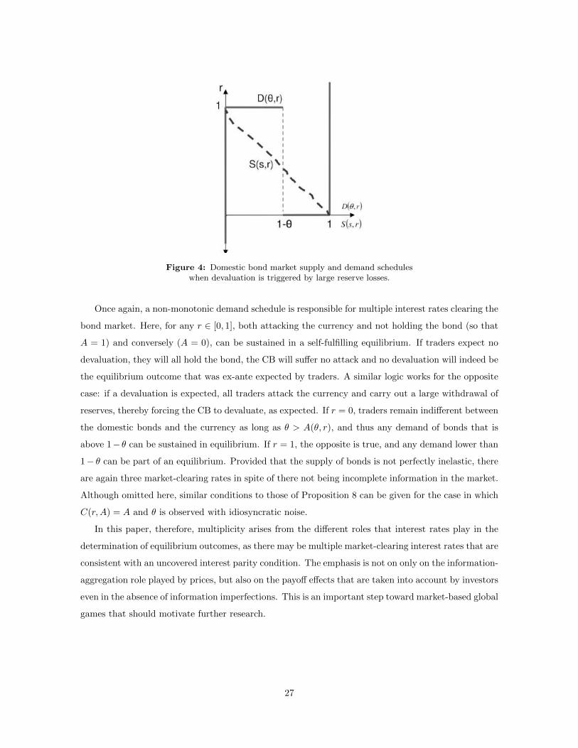
Figure 4: Domestic bond market supply and demand schedules

when devaluation is triggered by large reserve losses.

Once again, a non-monotonic demand schedule is responsible for multiple interest rates clearing the

bond market. Here, for any r 2 [0, 1], both attacking the currency and not holding the bond (so that

A = 1) and conversely (A = 0), can be sustained in a self-fulfilling equilibrium. If traders expect no

devaluation, they will all hold the bond, the CB will su↵er no attack and no devaluation will indeed be

the equilibrium outcome that was ex-ante expected by traders. A similar logic works for the opposite

case: if a devaluation is expected, all traders attack the currency and carry out a large withdrawal of

reserves, thereby forcing the CB to devaluate, as expected. If r = 0, traders remain indi↵erent between

the domestic bonds and the currency as long as ✓ > A(✓, r), and thus any demand of bonds that is

above 1� ✓ can be sustained in equilibrium. If r = 1, the opposite is true, and any demand lower than

1� ✓ can be part of an equilibrium. Provided that the supply of bonds is not perfectly inelastic, there

are again three market-clearing rates in spite of there not being incomplete information in the market.

Although omitted here, similar conditions to those of Proposition 8 can be given for the case in which

C(r, A) = A and ✓ is observed with idiosyncratic noise.

In this paper, therefore, multiplicity arises from the di↵erent roles that interest rates play in the

determination of equilibrium outcomes, as there may be multiple market-clearing interest rates that are

consistent with an uncovered interest parity condition. The emphasis is not on only on the information-

aggregation role played by prices, but also on the payo↵ e↵ects that are taken into account by investors

even in the absence of information imperfections. This is an important step toward market-based global

games that should motivate further research.

27

3.3 The role of equilibrium outcomes as signaling devices

Section 3.2 has outlined examples of global games in which the existence of a Walrasian market

provides meaningful information about economic fundamentals that help break down the uniqueness

results from Section 3.1. In this subsection we analyze a di↵erent source of endogenous public infor-

mation: the signaling role of ex-ante public policies and of equilibrium outcomes.

3.3.1 Angeletos, Hellwig and Pavan (2006): Policy as a signal for the investors

Up until this point, we have assumed the decision of the policy-maker to be straightforward: the

status quo is abandoned if the cost of the attack (be it in terms of size or interest rates) is too large

compared to the gains from maintaining the regime, given by the fundamental ✓. It is reasonable to

believe that governments design more sophisticated policies when faced with an economy-wide attack.

In the application to currency crises, a central bank can try to prevent an attack by undertaking

costly ex-ante policies such as borrowing reserves from abroad, placing taxes on capital outflows and

so forth. However, if made public before the game is played, such costly policies may in turn signal a

high probability of regime fragility, reduce investor’s strategic uncertainty and generate informational

feedbacks between public and private policies that may a↵ect equilibrium outcomes in critical ways

and, in some cases, force the very policies that were designed to defend the peg to become unwarranted.

To gain intuition, consider the following extension of our baseline game from Section 3.1. The

population of traders, their objectives and choice sets are identical to those seen above. The only

modification is on the policy-maker’s (PM) side. For simplicity, consider that nature draws ✓ from a

uniform distribution on the real line, and suppose that prior to the Morris and Shin game the PM

learns ✓ and chooses a policy, here the opportunity cost c 2 [c, c] ⇢ (0, 1) that the investors must bear

in the second stage for attacking the status quo. The payo↵ of the PM is

U

PM

(R, ✓, c, A) = (1�R)(✓ �A)� (c)

where as usual R denotes the regime outcome (with R = 1 meaning that the status quo is aban-

doned), A 2 [0, 1] is the size of the attack and (·) is a policy cost function, with

0(·) > 0 and

(c) = 0. Since choosing c = c entails no cost, so we will call this outcome an “inactive policy”. Any

choice c > c entails an “active policy”.

Once the PM has chosen its policy, c becomes common knowledge and the Morris and Shin game

starts: each agent i receives a signal xi

= ✓ + ⇠

i

with ⇠i

⇠ N (0, 1/�) and must choose a

i

2 {0, 1} to

maximize U

i

= a

i

(R� c).

Finally, the PM will observe the size of the attack A, and the regime outcome R will be realized.

In particular, the status quo will be abandoned if and only if UPM

(1, ·) � U

PM

(0, ·), which once again

28

means that

R(✓) = 1[A>✓]

and allows us to write the PM’s ex-post objective as

U

PM

(✓, c, A) = max{0, ✓ �A}� (c)

The following describes an equilibrium of this economy:

Definition 3 A symmetric Perfect Bayesian Nash equilibrium consists of a strategy for the PM, c :

R ! [c, c], a (symmetric) strategy for the agents, a : R⇥ [c, c] ! {0, 1}, and a c.d.f., µ : R⇥R⇥ [c, c] !

[0, 1], such that

c(✓) 2 arg maxc2[c,c]

U

PM

(✓, c, A(✓, c))

a(x, c) 2 arg maxa2{0,1}

a

Z +1

�11[A(✓,c)>✓]dµ(✓|x, c)� c

�

where µ(✓|x, c) is obtained from c(·) using Bayes’ rule and

A(✓, c) ⌘Z +1

�1a(x, c)

p��(

p�(x� ✓))dx

R(✓) ⌘ 1[A(✓,c(✓))>✓]

are, respectively, the equilibrium size of the attack and regime outcome, for any ✓ 2 R and c 2 [c, c].

A first point to note is that the Morris and Shin game of Section 3.1 is a particular case of the

Angeletos, Hellwig and Pavan (2006) economy in which c = c. That is, our baseline economy can

be viewed as one in which policy is not costly, uninformative and, therefore, ine↵ective. Suppose in

contrast that c < c, which means that there is a meaningful scope for informationally-relevant policy.

Then, the following result is reached:

Proposition 9 Suppose c < c. There are multiple equilibria:

1. There is an equilibrium in which c(✓) = c for all ✓, a(x, c) = 1[x<x

⇤(c)], and R(✓) = 1[✓<✓

⇤(c)],

where

x

⇤(c) = ✓

⇤(c) +��1(✓⇤(c))p

�

(12)

✓

⇤(c) = �⇣p

�(x⇤(c)� ✓

⇤(c))⌘= 1� c

29

2. For any c

⇤ 2 (c, c], there is an equilibrium in which a(x, c) = 1[x<x or (x,c)<(x̃,c⇤)], R(✓) = 1[✓<✓̃]

and

c(✓) =

8><

>:

c

⇤ if ✓ 2 [✓̃, ˜̃✓]

c otherwise

where x̃, ✓̃ and˜̃✓ are given by

✓̃ = (c⇤)

˜̃✓ = ✓̃ +

1p�

��1

✓1� c

1� c

✓̃

◆� ��1(✓̃)

�

x̃ = ˜̃✓ +

��1(✓̃)p�

Proof: In Angeletos, Hellwig and Pavan (2006), page 470. ⌅

Proposition 9 identifies two classes of equilibria. In the first class, the policy remains inactive: the

PM avoids the costs of policy by setting c(✓) = c for any ✓ and the same equilibrium outcome as in

the baseline game of Section 3.1 surfaces. In the second class of equilibria, however, the PM actively

uses the policy at a direct cost (c(✓)) > 0. When doing so, the policy choices convey information

to the agents about the economic fundamentals and there is feedback e↵ects that have been ex-ante

taken into account by both sides of the economy.

• The PM’s side: On the one hand, the PM understands from (12) that, relative to a benchmark

in which the policy remains idle (here, c = c), a higher c means that there is a smaller range of

values of ✓ for which the status quo must be abandoned. A myopic PM would use this fact to try

to reduce the size of the attack. A sophisticated PM like the one assumed by our definition of a

PBE, however, acknowledges the informational contents of such a policy. In particular, the said

policy would render e↵ective only for certain intermediate values of ✓. Indeed, if ✓ is too low (in

particular, ✓ < ✓̃), the direct cost (c) of information for deviating from the inactive benchmark

toward some c > c would exceed the indirect payo↵ gains from maintaining the status quo and

preventing an attack from being successful. If ✓ is too high (in particular, ✓ > ˜̃✓), the size of the

attack would otherwise (that is, if the policy were to remain unused) be too small to justify the

direct cost (c) of intervention. Therefore, only for intermediate values of ✓ can an active policy

survive. Formally, for any c

⇤ 2 (c, c], there is an equilibrium in which c(✓) = c

⇤ for any ✓ 2 [✓̃, ˜̃✓].

• The investors’ side: From the investors’ point of view, if they agree on a policy a(x, c) that

is insensitive to c, the PM’s policy would remain inactive. However, if they coordinate on a

30

strategy that is decreasing in c (less aggressive attacks when the cost of attacking is higher) and

✓ 2 [✓̃, ˜̃✓], then the PM can ex-ante decrease the size of the attack by raising c, as described in

the first bullet point, and less investors will indeed attack in equilibrium.

Multiplicity here is originated from the feedback e↵ects between the expectations of the PM re-

garding how sensitive the investor’s policy is to the policy, and reactions of investors to the information

embedded in those same policies. There is scope for multiplicity if agents are able to coordinate on

di↵erent interpretations of, and di↵erent reactions to, particular sets of policy choices, and if those in

turn induce di↵erent incentives to which the PM reacts optimally when choosing those policies.

3.3.2 Goldstein, Ozdenoren and Yuan (2011): Attacks as a signal for the policy-maker

In Angeletos, Hellwig and Pavan (2006), investors’ choices are a↵ected by ex-ante policy from the

policy-maker, which acts as a signal that may help reduce the size of speculative attacks in equilibrium.

It is reasonable to believe that the interaction can also go in the opposite direction, namely that

aggregate trading of speculators may reveal information to the central bank and a↵ect its policy

decision. Goldstein, Ozdenoren and Yuan (2011) study this aspect of the informational interaction

between market activities and policy decisions by allowing the central bank to learn from the very same

market complementarities that its policies generate. The fact that the central bank can learn from

market outcomes in order to perform inference about fundamentals, however, feeds right back into the

same market outcomes that may arise, for it facilitates further coordination between investors in the

same spirit as the ex-ante costly policy signaled the state of the economy in the approach followed by

Angeletos, Hellwig and Pavan. However, unlike in that paper, here the policy-maker is oblivious to

the realization of the fundamental when undertaking its policy, and observing a large attack on the

part of the investors may prove to be useful information about the underlying state of the economy.

The following is a concise description of the model. As usual, a continuum of speculators coexist

with a single policy-maker (PM). With a single exception noted below, the investors’ side is identical

to what we described in Section 3.1: they take a zero-one action, at a cost of c 2 (0, 1) for the active

action, upon the observation of unbiased signals about ✓. The PM decides whether or not to maintain

the status quo, and the economic fundamental ✓ stands for the value of maintaining it. The PM does

not observe the realization of ✓ when making a policy choice. We characterize the decision of the PM

as a variable � 2 {0, 1}, and its payo↵ as

U

PM

= �✓

Note that, unlike in all the settings discussed above, the PM is now not directly a↵ected by the size

of the attack. However, the investors’ decisions matter because they may provide information about ✓

31

to the PM.

The timing is as follows. First, both the PM and the speculators receive information about ✓. The

common prior is di↵use over the real line. The PM receives a private signal:

x

PM

= ✓ +⇠

PMp�

PM

where ⇠PM

⇠ N (0, 1). Each speculator i 2 [0, 1] receives two signals. One signal is as in the

benchmark model:

x

i

= ✓ +⇠

ip�

with ⇠i

⇠ N (0, 1). A second signal is also private but includes a noise component that is commonly

shared by all speculators:

x

pi

= ✓ +⇠

pp↵

+⌘

ip⌧

where ⇠p

⇠ N (0, 1) is the common noise component and ⌘i

⇠ N (0, 1) is the private noise component.

The terms �, �PM

, ↵ and ⌧ all denote precisions. The precision of xpi

is ⌧ 0 = ↵⌧/(↵ + ⌧). All error

terms are orthogonal to one another. The commonly shared component in the second signal implies

that this signal is correlated across speculators12. Once the agents independently gather these sources

of information, speculators simultaneously decide whether or not to attack the status quo. Finally,

after observing the size of the attack, the PM decides whether or not to abandon the regime. The

payo↵s and information structure are common knowledge, but the true realization of ✓ is not observed

at any point of the game.

Each individual speculator is not identified by a pair of signals, and as usual we drop i subscripts.

The following defines the equilibrium.

Definition 4 A symmetric Perfect Bayesian Nash equilibrium consists of a strategy for the PM,

�(A, xPM

), a symmetric strategy for the speculators, a(x, xp

), a size of the aggregate attack A(✓, ⇠p

),

and posterior probability measures ⌫(✓|A, x

PM

) for the PM and µ(✓|x, xp

) for the speculators, such

that

• Decisions are optimal given the information sets:

12One way of motivating this, as viewed by the authors, is to think of the information generating process as beingsubject to common random shocks such as market-wide rumors.

32

�(A, xPM

) 2 arg max�2{0,1}

Z +1

�1�✓d⌫(✓|A, x

PM

)

a(x, xp

) 2 arg maxa2{0,1}

a

Z +1

�1

Z +1

�11[�(A(✓,⇠

p

),✓+⇠

PM

/

p�

PM

)=0]dµ(✓|x, xp

)�(⇠PM

)d⇠PM

� c

�

A(✓, ⇠p

) = ��1

✓Z +1

�1

✓Z +1

�1a(✓ + ⇠/

p�, ✓ + ⇠

p

/

p↵+ ⌘/

p⌧)�(⌘)d⌘

◆�(⇠)d⇠

◆

• Beliefs are consistent in the sense that ⌫(✓|A, x

PM

) is obtained using Bayes’ law for any A and

x

PM

, and µ(✓|x, xp

) is also obtained using Bayes’ law for any x and x

p

.

The following proposition states that the PBE is in threshold strategies: there exist cuto↵s levels

denoted {x⇤(xp

), A⇤(xPM

)} such that a speculator attacks the status quo if x x

⇤(xp

) and the PM

in turn abandons the regime if A � A

⇤(xPM

). Moreover, these thresholds are uniquely defined.

Proposition 10 There is a unique linear threshold equilibrium in which the speculators’ optimal strat-

egy is a(x, xp

) = 1[xx

⇤(xp

)] and the PM’s optimal strategy is �(A, x

PM

) = 1[AA

⇤(xPM

)], where

x

⇤(xp

) = x

⇤(0)� kx

p

A

⇤(xPM

) =1q

1�

+ k

2

⌧

x

⇤(0) + (1 + k)�

PM

�

T

x

PM

�

k is the unique real root to the cubic equation

✓⌧k

2 � �

↵

(⌧ + ↵)k3◆�

PM

+ ↵(1 + k)2(⌧ � �k) = 0

and

�

T

⌘ ↵

✓1 +

1

k

◆2

is the precision of the attack as a signal of the fundamental.

Proof: In Goldstein, Ozdenoren and Yuan (2011), page 270. ⌅

Note that the investors’ signal is decreasing in the correlated signal xp

, which o↵ers a source of

public information. When x

p

indicates a sound fundamental, speculators attack only if their own

private and independent signal, x, o↵ers particularly pessimistic information about ✓. The weight

that the speculators put on the correlated signal is k � 0 and it spills over to the PM’s decision, who

33

anticipates the investors’ attacking rule. Indeed, the PM infers the underlying state of the economy

from observing attacks, and �T

, which represents the precision the attack as a signal of the fundamental,

is decreasing in k: when investors put more weight on the source of information that is shared by others,

an attack becomes less informative for the PM.

However, investors anticipate the information transmission e↵ects that their attacks carry over to

PM’s policies. In particular, since they internalize that the likelihood of a successful attack is increasing

in the precision of the PM’s attack-signal, which is in turn decreasing in the weight k they place on

the commonly shared piece of information, investors end up putting “too much” weight on x

p

, that

is, a higher weight than that which would be used in an economy in which the PM could not infer

information about ✓ from the size of the attack13. Intuitively, when a single speculator places more

weight on x

p

, other speculators follow because not only this signal provides more information about

the true ✓, but also because it a↵ects the likelihood of a large-scale attack being successful through

the signaling power of the size of the attack.

In this sense, the central conclusion is reminiscent of the Morris and Shin (2002) result regarding

the detrimental value of public information, with the only di↵erence that whereas in that set-up

informational complementarities emerged from payo↵ complementarities (in particular, a Keynesian

beauty-contest type of game), in the present framework such complementarities arise endogenously

through the feedback e↵ects of policy and the fact that both sides of the economy learn from one

another. Overall, the very informational complementarities that are responsible for the investors

choosing to overweight the commonly shared signal are the ones that generate large attacks that are

not justified by bad fundamentals14.

3.4 Dynamic models of global games

Section 3.2 has shown that the celebrated uniqueness result from Carlsson and van Damme (1993)

and Morris and Shin (1998) is extremely fragile to the information structure of the game. We have

outlined two examples, prices as information aggregators and equilibrium actions as signaling devices,

under which uniqueness may vanish because the possibility of exploiting additional endogenous strate-

gic complementarities fosters coordination back to multiplicity. This section proposes a third route:

while all the models analyzed above are static, one can generate public information by allowing agents

to make use of past outcomes and learn from their own actions in dynamic games of regime change.

There has been a substantial amount of work in dynamic coordination games over the past few years.

Frankel and Pauzner (2000), Burdzy, Frankel and Pauzner (2001) and related papers study coordination

13This is the statement of Proposition 2 in their paper, proved in page 273.14A number of interesting policy implications, including e↵ectiveness and transparency, can be drawn from this result

alone, but I will left these out for the sake of exposition. The interested reader is referred to sections 5 and 6 of theoriginal paper.

34

games in which players are randomly matched into two-player, two-action dynamic games where the

fundamental evolves according to a random process and players can revise their actions according

to a Poison arrival process. In Levin (2000), at each point in time payo↵s may depend on actions

chosen by past players, by future players, and on fundamentals, where the payo↵ parameter evolves

according to a random walk and is announced publicly15. Matsui (1999) and Oyama (2004) assume

complementarities between actions of successive generations in respective OLG models of coordination.

In an approach loosely related to the global games view, the herding and social learning literature (e.g.,

Banerjee (1992) and Bikhchandani, Hirschleifer and Welch (1992)) assumes that players sequentially

make discrete choices and partially learn the information of players who choose before them.

Strictly within the dynamic global games literature, Chamley (1999, 2003) considers dynamic

global games with recurrent incomplete information, Chassang (2010) studies the e↵ects of the fear of

misscoordination on the sustainability of cooperation in a dynamic game with exit and Giannitsarou

and Toxvaerd (2012) outline a recursive formulation of general dynamic global games and characterize

Markov equilibria. Dasgupta (2007) provides a model of private social learning in which the dynamics

are augmented by endowing the agents with the option to delay their decisions at a cost, and analyzes

the welfare implications of a broad class of games.

I have chosen to review three papers that I consider relevant and build up naturally on one another.

I will start with Morris and Shin (1999), an arguably straightforward dynamic extension of Morris and

Shin (1998) in which the fundamental is revealed at the end of every period. I will then move on

to Angeletos, Hellwig and Pavan (2007), who give a characterization of a similar game in which the

underlying fundamental is fixed and learned only in the limit of time. Finally, I will review Steiner

(2008), who proposes a recursive formulation of a dynamic game in which agents can influence their

own participation in future rounds. All three papers have in common that the threshold equilibrium

properties discussed above extend naturally to the dynamic setting, and in some cases the uniqueness

result from the stage game is preserved in the multi-stage set-up. Because past outcomes may become

public information, which restores common knowledge, multiplicity may resurrect and will be once

again a recurrent theme. However, because in some instances players never learn the true realization

of the state, the size and number of future possible attacks remains ambiguous and, in some cases,

entirely unpredictable.

3.4.1 Morris and Shin (1999): A repeated static global game

To set firm ground from which to start building dynamics, let us begin with a repeated-game

version of Morris and Shin (1998): a stage game played over and over with periodical disclosure of the

fundamental of the economy.

15In related work, Levin (2001) studies a similar set-up with overlapping generations of players.

35

Time is continuous and t = �, 2�, 3�, . . . denotes each instant, where � > 0 is negligibly small.

The fundamental of the economy at instant t, called ✓t

, evolves according to a Brownian motion, so

that

d✓

t

= z

p�dt

where z ⇠ N (0, 1). On each period t, the benchmark game of Section 3.2 is played: each speculator

i 2 [0, 1] receives a signal xit

= ✓

t

+ ⌘

i

, with ⌘i

⇠ N (0,�/�), and chooses an action a

it

2 {0, 1}. The

PM, who observes ✓t

noiselessly, will abandon the status quo if and only if A

t

� ✓

t

, where A

t

is

the aggregate size of the attack. The true value of the fundamental at instant t becomes common

knowledge at the end of the period, when all actions have been realized. Therefore, the information

set of the PM at the beginning of period t is {✓t

}, and the information set of the speculators at the

beginning of period t is {✓t��, x

t

i

}, where x

t

i

⌘ {xi,�, xi,2�, . . . , xit

} is the history of signals16. The

definition of equilibrium is a straightforward extension of Morris and Shin (1998), and therefore is

omitted here.

The characterization of the main equilibrium dynamics is given by the following proposition:

Proposition 11 For a su�ciently high �, there exists a stochastic process ht

⌘ h(✓t

) with the property

h

t

� h

t�� if ✓t�� ✓

t�2�

such that the equilibrium regime outcome is given by R(✓t

) = 1[✓t

h

t

].

Proof: In Morris and Shin (1999). ⌅

This proposition shows that the onset of an successful attack can be succinctly characterized by

the fundamentals “tripping over” a hurdle process that moves in the opposite direction as the first-

lagged underlying state. This implies that the prospect of a currency attack increases more than

proportionately to a decrease in the fundamentals. Intuitively, the evolution of beliefs which trigger

the change of sentiment and, in turn, precipitate the attack can be again represented by a (time-varying)

threshold policy: when � is large, private information has a higher quality and speculators put more

weight on the last fundamental they observed (call it ✓��) and more on their contemporaneous signal,

x

t

. If fundamentals are thought to deteriorate, the indi↵erent speculator believes other speculators to

be more likely to unilaterally attack, and therefore a coordinated attack to be more likely to succeed.

16Clearly, since ✓t

is commonly observed at the end of each period t, all signals that the trader has received up to thatpoint become uninformative, and are therefore discarded in the individual inference problem.

36

Indeed, the hurdle process then increases and the PM is more likely to abandon the status quo in

equilibrium, as expected ex-ante by the speculators.

3.4.2 Angeletos, Hellwig and Pavan (2007): Endogenous dynamics and timing of attacks

An extreme simplification of the approach just laid out is that ✓t

is revealed to the private agents

at the end of each period, permitting them to discard past signals and, loosely speaking, turning the

problem into an infinitely repeated static game rather than a game with dynamic inter-temporal inter-

actions. Angeletos, Hellwig and Pavan (2007) show that dropping the periodical disclosure assumption

is crucial for obtaining a much richer understanding of the equilibrium dynamics. Indeed, in this case,

since past signal realizations are informative about the fundamental (as long as the latter is somewhat

persistent or, in their example, just constant), there is scope for learning over time. Moreover, the

game continues for as long as the status quo is in place, which in turns o↵ers an additional source of

public information from which agents can learn and form future action profiles.

In this model, time is discrete and runs to infinity. Once again, consider a Morris and Shin (1998)

game played repeatedly period after period. A fundamental ✓ 2 R is drawn by nature at the beginning

of time from ✓ ⇠ N (z, 1/↵). The PM observes this fundamental, but the population of traders does

not. Instead, each trader i 2 [0, 1] receives a signal

x̃

it

= ✓ + ⇠

it

each period t, where ⇠it

⇠ N (0, 1/⌘t

). The PM abandons the status quo at time t if At

> ✓, so

R

t

= 1[At

>✓] is the period-t regime outcome. The game ends once and for all when the status quo is

first abandoned. Speculator i’s payo↵ from the entire game is

⇧i

=+1X

t=1

�

t�1(1�R

t

)⇡it

where � 2 (0, 1) is a time discount factor and ⇡it

is an instantaneous payo↵ function, given by

⇡

it

= a

it

(Rt+1 � c)

where c 2 (0, 1) is the opportunity cost of attacking and a

it

2 {0, 1} is the action chosen in period

t. Note that this specification is a natural dynamic extension of the static payo↵s defined in Section

3.1.

Conditional on the status quo being at place at the beginning of period t, let a

t

: Rt ! [0, 1] be

the strategy for period t, at

⌘ {a⌧

}t⌧=1 be the strategy profile up to period t (with a

1 ⌘ {a⌧

}+1⌧=1),

p

t

(✓; at

) be the probability that the status quo is abandoned in period t when all agents follow strategy

37

a

t

and t

(✓|x̃t; at�1) be the c.d.f. of posterior beliefs in period t, where x̃

t ⌘ {x̃⌧

}t⌧=1. The following

describes an equilibrium:

Definition 5 A strategy a

1 is part of a symmetric monotone Perfect Bayesian Nash equilibrium if

a

t

(xt) is non increasing in x

t and independent of past actions, and is such that

a1(x̃1) 2 arg maxa2[0,1]

a

Z +1

�1p1(✓; a1)d 1(✓|x̃1)� c

�

for all x̃1 2 R and, at any t � 2,

a

t

(x̃t) 2 arg maxa2[0,1]

a

Z +1

�1p

t

(✓; at

)d t

(✓|x̃t; at�1)� c

�

for all x̃t 2 Rt.

Since traders never observe the fundamental ✓ perfectly, they must keep track of their entire history

of signals. This is duly reflected in the definition of equilibrium above. However, it turns out that a

convenient recursive representation can be used in this case. To see this, define

�

t

⌘tX

⌧=1

⌘

⌧

to be the cumulative private precision. It is not di�cult to see that if �t

� ↵

2

2⇡ , the stage game

will have a unique solution17. Moreover, assume that limt!+1 �

t

= +1, meaning that the perfect

information benchmark takes place only in the limit of time, but that ✓ is uncertain for the investors

in any finite time. To formulate the problem recursively, define

x

t

=�

t�1xt�1 + ⌘

t

x̃

t

�

t

and �

t

= �

t�1 + ⌘

t

for any t � 2, with �1 = ⌘1 and x1 = x̃1. Then, posterior beliefs ✓|x̃t can be conveniently written

in terms of current-period variables as follows:

✓|x̃t ⇠ N✓�

t

x

t

+ ↵z

�

t

+ ↵

,

1

�

t

+ ↵

◆

Namely, we have found x

t

to be a single su�cient statistic for the whole history of signals x̃t with

respect to ✓ and R

t+1. All private information being summarized in a single-dimensional object reduces

the dimensionality of the problem immensely, and it is due to the Bayesian-step Gaussian updating

and the additive structure of signals.

17This is a direct extension of Proposition 3 in Section 3.1.

38

The following proposition shows that an equilibrium may still be represented by (time-varying)

thresholds of attack and devaluation:

Proposition 12 Any monotone equilibrium is characterized by a sequence {x⇤t

, ✓

⇤t

}+1t=1 with x

⇤t

2 R [

{�1}, ✓⇤t

2 (0, 1) and ✓⇤t

� ✓

⇤t�1, such that:

1. At any t, an agent attacks if and only if xt

< x

⇤t

, and otherwise the agent refrains from attacking.

2. The status quo is in place in period t if and only if ✓ > ✓

⇤t�1. Otherwise, the game ends.

Proof: In Angeletos, Hellwig and Pavan (2007), page 722. ⌅

As in the static version of the game, each period ✓⇤t

and x

⇤t

⌘ X(✓⇤t

,�

t

) solve ✓⇤t

= A

t

(✓⇤t

) = P[xt

x

⇤t

|✓⇤t

], that is,

✓

⇤t

= ��p

�

t

(x⇤t

� ✓

t

)�

and the indi↵erent condition for the marginal trader:

P[✓ ✓

⇤t

|x⇤t

, ✓ > ✓

⇤t�1] = c

Clearly, since by construction of the game the agents can choose an action only if the status quo

has never been abandoned in past periods, {✓⇤t

} is a non-decreasing sequence in time: the status quo

cannot be in place in a certain period without it also being in place in the previous period. The

evolution of x⇤t

will critically determine, however, the size of the attacks in equilibrium. Interestingly,

{x⇤t

} need not be monotonic, and therefore periods in which some agents might attack (x⇤t

> �1)

may alternate with periods in which nobody attacks (x⇤t

= �1).

To understand more deeply the dynamics of attack, the authors propose the following alternative

specification by shifting the focus of the study to the conditions of the marginal indi↵erent trader,

i.e. the agent with signal xt

= X(✓⇤t

,�

t

). Let U(✓⇤t

, ✓

⇤t�1,�t,↵, z), sometimes U

MG

t

for brevity, be

the net payo↵ from attacking in period t for this agent. To construct this function, first define

u : R⇥ [0, 1]⇥ R⇥ R2+ ⇥ R ! [�c, 1� c] and X : [0, 1]⇥ R+ ! R by

u(x, ✓⇤, ✓⇤�1,�,↵, z) ⌘

8><

>:

1� �(p�+↵( �x+↵z

�+↵

�✓

⇤))�(

p�+↵( �x+↵z

�+↵

�✓

⇤�1))

if ✓⇤ > ✓

⇤�1

�c if ✓⇤ ✓

⇤�1

X(✓⇤,�) ⌘ ✓

⇤ +��1(✓⇤)p

�

39

respectively, and so the marginal trader’s utility function U : [0, 1]⇥ R⇥ R2+ ⇥ R ! [�c, 1� c] is

U(✓⇤, ✓⇤�1,�,↵, z) ⌘

8>>>><

>>>>:

limx!�1 u(x, ✓⇤, ✓⇤�1,�,↵, z) if ✓⇤ = 0

u(X(✓⇤,�), ✓⇤, ✓⇤�1,�,↵, z) if ✓⇤ 2 (0, 1)

limx!+1 u(x, ✓⇤, ✓⇤�1,�,↵, z) if ✓⇤ = 1

Here, u(x, ✓⇤, ✓⇤�1,�,↵, z) is the net payo↵ from attacking in period t if the agent receives signal x,

when it is known that the status quo is still in place (✓ > ✓

⇤�1) and that the regime will change if and

only if ✓ ✓

⇤; X(✓⇤,�t

) is the threshold x

⇤ such that, if agents attack in period t if and only if xt

x

⇤,

then A

t

(✓) � ✓ if and only if ✓ ✓

⇤; U(✓⇤, ✓⇤�1,�t↵, z) is again the net payo↵ from attacking for the

marginal agent with signal x⇤ = X(✓⇤,�t

) when it is known that ✓ > ✓

⇤�1. Clearly, since X(✓⇤,�) is

the solution to ✓⇤ = A(✓⇤) (that is, to ✓⇤ = �(p�(x⇤ � ✓

⇤)) for x⇤ being the individual attack cuto↵

level), then (✓⇤t�1, ✓

⇤t

) belongs to the equilibrium path if and only if

U(✓⇤t

, ✓

⇤t�1,�t,↵, z) = 0

This representation allows us to draw several important results, which I summarize in the next

three central propositions. The first one, Proposition 13, presents existence of the threshold paths and

o↵ers a recursive algorithm to find them.

Proposition 13 The strategy a

1 is a monotone equilibrium if and only if there exists a sequence of

thresholds {x⇤t

, ✓

⇤t

}+1t=1 such that

1. For all t, at

(x̃t) = 1 if xt

< x

⇤t

and a

t

(x̃t) = 0 if xt

> x

⇤t

.

2. For t = 1, ✓⇤1 solves U(✓⇤1 ,�1,�1,↵, z) = 0 and x

⇤1 = X(✓⇤1 ,�1).

3. For any t � 2, either ✓⇤t

= ✓

⇤t�1 > 0 and x

⇤t

= �1, or ✓⇤t

> ✓

⇤t�1 > 0 is a solution to

U(✓⇤t

, ✓

⇤t�1,�t,↵, z) = 0 and x

⇤t

= X(✓⇤t

,�

t

).

A monotone equilibrium always exists.

Proof: In Angeletos, Hellwig and Pavan (2007), page 745. ⌅

What this proposition states is that learning takes the form of a truncation in the support of

beliefs about ✓. Upon the observation that the regime has survived past attacks, the agents acquire

the knowledge that ✓ is above a threshold ✓⇤t�1. Moreover, the results provides a recursive algorithm

to compute equilibria. Note that U(✓⇤1 ,�1,�1,↵, z) = 0 admits a solution, and there is at least one

monotone equilibrium in this economy. One way of constructing all other equilibria is to initialize the

40

algorithm at this first-period solution, ✓⇤1 , and move forward in time. At t = 2, if U(✓2, ✓⇤1 ,�2,↵, z) = 0

admits no solution for ✓2, we set ✓⇤2 = ✓

⇤1 , and if a solution ✓⇤2 exists, then ✓2 2 {✓⇤1 , ✓⇤2}. Moving forward,

one can construct potentially all the equilibrium paths {✓⇤t

}+1t=1 , together with the corresponding

thresholds {x⇤t

}+1t=1 .

Proposition 14 states more formally that there may be multiplicity of equilibria in this environment:

Proposition 14 The following are features of the equilibrium set, for any t 2 Z+:

1. U(✓⇤t

, ✓

⇤t�1,�t,↵, z) is continuous in all its arguments, non-monotonic in ✓

⇤t

when ✓

⇤t�1 2 (0, 1),

and strictly decreasing in ✓⇤t�1 and z for ✓⇤

t�1 < ✓

⇤t

.

2. Let ✓̂t

be the unique solution to U(✓̂t

,�1,�

t

↵, z) = 0. A solution to U

t

(✓⇤t

, ✓

⇤t�1,�t,↵, z) = 0

exists only if ✓⇤t�1 < ✓̂

t

, and is bounded from above by ✓̂t

.

3. If ✓⇤t�1 > 1� c, a solution to U

t

(✓⇤t

, ✓

⇤t�1,�t,↵, z) = 0 does not exist for �

t

su�ciently high.

4. If ✓⇤t�1 < 1� c, a solution to U

t

(✓⇤t

, ✓

⇤t�1,�t,↵, z) = 0 necessarily exists for �

t

su�ciently high.

5. If ✓⇤t�1 is the highest solution to U

t�1(✓⇤t�1, ✓

⇤t�2,�t�1,↵, z) = 0, there exists a � > �

t�1 such

that Ut

(✓⇤t

, ✓

⇤t�1,�t ↵, z) = 0 admits no solution for any ⌧ � t such that �

⌧

< �.

An implication of points 1 and 2 of this proposition is that UMG is flat at �c for ✓⇤t

< ✓

⇤t�1, then

increases with ✓⇤t

, and eventually decreases with ✓⇤t

by converging again to �c as ✓⇤t

goes up. Every

intersection of the function with the horizontal axis corresponds to a solution. The non-monotonicity

therefore leaves open the possibility for multiplicity of equilibria. Parts 3, 4, and 5 highlight that

agents must have accumulated precise enough private information up to a given period for further

attacks to be possible after that period. Only under such a parameter condition future attacks may

emerge in equilibrium. If this does not hold for any period, a first-period attack is the only equilibrium

of the economy.

Intuitively, on the one hand, the knowledge that the regime has survived past attacks (inferred

from the observation that the game has not ended) operates as a deterrent motive for agents to attack,

and even more so if they expect other agents not to attack, either. Whether or not future attacks can

take place also then depends in critical ways on the mean common prior, z.

• If the common prior z is low, this motive is reinforced, for the perceived probability of regime

change is low and the net payo↵ from attacking for the marginal agent is low. In that case, a

unique equilibrium of the entire game exists in which an attack occurs only in the first period.

• In contrast, if the accumulated private information is precise enough, a su�ciently high z can

o↵set said deterrent motive: a positive prior belief about the fundamental raises optimism over

41

and above adverse incentives stemming from the knowledge that past attacks failed to succeed,

and make the economy prone to further attacks.

Figure 5 illustrates a particular example in which this second case holds. The figure depicts the

utility of the marginal agent for period 1 (dashed line), period 2 (dotted line) and period 3 (solid line).

Note that the dashed line crosses the horizontal axis once, meaning that there is always an attack

in the first period. The parametrization is such that no attacks are possible in period 2, due to a

combination of a low �2 relative to z: agents have not yet acquired enough private information about

the fundamental, and z is not high enough to convince them that an attack is worthwhile even if the

first-period one failed to succeed. In period 3, however, the private signal is precise enough to make

a second attack possible. Moreover, by Proposition 14, a third attack is possible at some future date.

In terms of the evolution of thresholds ✓⇤t

, three possible sequences can be constructed by means of

the algorithm outlined in Proposition 13: either ✓⇤t

= ✓

⇤1 , 8t � 2; or ✓⇤2 = ✓

⇤1 and ✓⇤

t

= ✓

03, 8t � 3; or

✓

⇤2 = ✓

⇤1 and ✓⇤

t

= ✓

003 , 8t � 3.

Figure 5: An example of equilibria with multiple attacks. The dashed line is the payo↵

for the marginal agent in period 1, the dotted line is his payo↵ in period 2,

and the solid line is the payo↵ in period 3. Notation: ✓1 ⌘ 1� c.

The next proposition formalizes these intuitions regarding the mean prior.

Proposition 15 There exist thresholds z z z such that

1. If z < z, there is a unique monotone equilibrium and it is such that an attack occurs only in

period one.

2. If z 2 (z, z), there are at most finitely many monotone equilibria and 9t < +1 such that, in any

of these equilibria, no attack occurs after period t.

42

3. If z > z, there are infinitely many equilibria and if, in addition, z > z, for any (t,N) 2 Z2+ there

is an equilibrium in which N attacks occur after period t.

Finally, z = z = z when c 1/2, whereas z z < z when c > 1/2.

Proof: In Angeletos, Hellwig and Pavan (2007), page 728. ⌅

At least two important corollaries can be drawn from this result. First, if ✓ > 1 � c and z > z,

the status quo survives in any equilibrium. However, for any t > t and some t 2 Z+, an attack (or

any number of them, for that matter) can occur yet does not necessarily take place. An important

consequence of this is that neither the timing nor the number of attacks can be predicted.

Furthermore, after the most aggressive attack for a given period takes place, the game enters a phase

of tranquility, during which no attack is possible, and the length of which is decreasing in the speed

of arrival of private information. Hence, in equilibrium, there may exist cycles of repeated succession

of phases of tranquility, during which no attack occurs, and phases of distress, which conclude after a

strong though failed attack on the status quo. This theme will reappear in section 3.4.3.

I conclude this exposition with two final remarks. First, note that coordination cycles emerge

purely from the interaction between coordination and information, and not from any change in the

underlying fundamental. This dimension was completely ignored by Morris and Shin (1999), who

could not disentangle fundamental e↵ects from informational e↵ects. Second, observe that the source

of the dynamics is extremely sensitive to the cumulative private precision �

t

, for a small change in

this parameter from one period to another can trigger the switch from tranquility to distress. This

discontinuity in outcomes with respect to changes in information is reminiscent of nonfundamental

volatility as a source of regime instability, as for instance in Angeletos and Werning (2006) (recall our

discussion of Proposition 4).

3.4.3 Steiner (2008): Coordination cycles through the role of participation

Angeletos, Hellwig and Pavan (2007) is a stylized example of how global games settings can generate

cycles of coordination that can lead to di↵erent patterns of equilibria even in the absence of exogenous

fluctuations of economic fundamentals. In that example, the link between periods is encoded in

the ability of players to transform the knowledge that the regime has survived in past rounds into

knowledge about the soundness of the fundamental. This endogenous and inter-temporal transmission

of information explains why agents may consider worthwhile to postpone their attack decisions. But

because di↵erent agents can agree on di↵erent interpretations and di↵erent reactions to the same

equilibrium outcomes, coordination cycles of uncertain length and strength emerge eventually as new

private information arrives exogenously.

43

Steiner (2008) refines this idea18. In his example, the dynamic link between periods is that each

player influences, with the choice of her current action, not only her instantaneous payo↵ but also her

own future participation in the game. The risky action (attack) is risky not only because it pays o↵ if

and only if su�ciently many agents undertake it, but also because it can otherwise lead to bankruptcy

and prevent the agent to participate in future projects. Individual and multilateral fear of bankruptcy

introduce additional strategic risk into the problem: future coordination undermines current coordi-

nation by making attacks more risky in the present round, which incorporates an additional feedback

e↵ect between adjacent periods that can lead to chaotic cycles and no steady-state convergence.

Here is a description of the model, once again adapted to the nomenclature introduced above. Time

is discrete and finite19, t = 1, . . . , T . The fundamental is now a stochastic i.i.d. process ✓t

with twice

continuously di↵erentiable c.d.f. �(·) on the real line. The realization ✓t

is revealed at the end of every

period t, but unknown through period t. Once more, each agent i receives an unbiased private signal

x

it

= ✓

t

+⇠

ip�

where the idiosyncratic errors ⇠i

are independent across players and rounds and drawn from a

continuous p.d.f. f(·) with support in the real line20. The focus will be on the perfect information

limit, where � ! +1.

Each agent in the continuum has to choose an action a

it

2 {0, 1}. Agent i’s payo↵ of the whole

game is

⇧i

=TX

t=1

�

t�1⇡

it

where � 2 (0, 1) is a factor of time discount and, in a slight abuse of notation, ⇡it

is an instantaneous

payo↵ function given by

⇡

it

⌘ a

it

⌧

it

⇡(✓t

, A

t

)

where A

t

is the measure of players choosing to attack, the marginal payo↵ ⇡(✓t

, A

t

) satisfies prop-

erties A1, A2, A3, A4, A5 and A6 listed in section 2.2.1 above21, and, as a novelty, ⌧it

� 0 is the degree

of agent i’s involvement into the game. Note that, unlike in Angeletos, Hellwig and Pavan (2007), the

18See also related work by Mathevet and Steiner (2013).19As we will see later on, finiteness is not essential except for the equilibrium uniqueness result. See Section 3.3 of

Steiner (2008) for a more detailed discussion.20We can think of the case ✓

t

⇠ iid N (z, 1/↵), as in Section 3.4.2, though the exposition is general enough toaccommodate any twice continuously di↵erentiable c.d.f. on the real line, �(·). Similarly, the idiosyncratic errors may,but need not, be normally distributed.

21Note that the specification ⇡(✓t

, At

) = 1[At

>✓

t

] � c for c 2 (0, 1), which we have used in all the models above, is aparticular example of one such function. Later on we will specialize this framework to the Morris and Shin game thatwe have repeatedly analyzed in this paper.

44

game does not end after a successful attack, and therefore regime switches constitute a dimension the

agents can learn from.

When taking ⌧it

as a fixed parameter, Propositions 1 in section 2.2.1 above state that each one of

the T static games of which the model is composed is a global game with a unique equilibrium that

can be solved by threshold strategies: for each t = 1, 2, . . . , there exists a ✓⇤t

such that the optimal

individual strategy at stage t is a(xit

) = 1[xit

�✓

⇤t

].

The dynamic link between the di↵erent stage games is that the involvement is endogenous. In

particular, ⌧it

is defined recursively by

⌧

i,t+1 = ⌧

it

b(ait

, ✓

t

, A

t

)

with b(ait

, ✓

t

, A

t

) � 0, and ⌧i1 = 1 is a normalization. If b

it

= 0, so that ⌧i,t+1 = 0, then the player

is not involved in the play of stage t + 1. From the perspective of period t, the function b(ait

, ✓

t

, A

t

)

can thus be interpreted as a continuation probability, and ⌧i,t+1 as expected participation next period.

Note that b(·) need not be bounded above by one, a case in which the player’s participation would

wear out over time. In contrast, high involvement benefits players because it allows them to take

advantage of accessing potentially higher payo↵s by waiting (i.e, choosing a = 1) while having the

zero-payo↵ outside option still available every period. Thus, withholding embeds a double reward: a

direct payo↵ e↵ect in the case of successful attack, and an augmented payo↵ e↵ect stemming from the

benefit of not having participated in rounds in which attacks were not successful.

To complete the description of the environment, we need a few more technical assumptions. Where

we define ⇢(✓t

, A

t

) ⌘ b(1, ✓t

, A

t

) � b(0, ✓t

, A

t

), we assume that ⇢(✓t

, A

t

) is weakly increasing in both

✓

t

and A

t

, andR 10 g(A)⇢(✓

t

, A)dA is continuous with respect to ✓t

, for any t 2 [T ], and densities g(·).

Moreover, we assume that the function

⇡̃(✓t

, A

t

) ⌘ ⇡(✓t

, A

t

) + �⇢(✓t

, A

t

)Vt+1

satisfies the uniform limit dominance condition (condition A4 in section 2.2.1) for any number

V

t+1 > 0. Finally, in order to keep the measure of players constant, it is assumed that the measure of

players who disappear from play at each period t (that is, the set {i : ⌧it

= 0} ✓ [0, 1]) is replaced by

an equal measure of entrants.

Let us formalize notation and derive the solution. We denote by V

t

the value of the game conditional

on participation at stage t. Under this notation, ⇡̃(✓t

, A

t

) ⌘ ⇡(✓t

, A

t

) + �⇢(✓t

, A

t

)Vt+1 is interpreted

as the period payo↵ di↵erential between attacking and refraining22. The information set of each agent

is Iit

⌘ {xt

i

, ✓

t

, a

t

i

} as of stage t 2 [T ], where superscripts denote histories. We call a pure strategy a

22Of course, ⇡̃(✓T

, AT

) = ⇡(✓T

, AT

) as the game ends after period T , that is, VT+1 = 0.

45

sequence s = (s1, . . . , sT ) of functions that assign to each pair of information sets (Ii1, . . . , IiT ) a path

of actions (s1(Ii1), . . . , sT (IiT )).

The solution method is by backward induction. At stage T , we know by Proposition 2 in section

2.2.1 above that the unique equilibrium of the stage game can be characterized by a threshold ✓⇤T

such

that s

⇤T

(x) = 1[x�✓

⇤T

]. As seen before, the threshold ✓⇤T

is such that s

⇤T

(·) is the best response to the

belief that a measure A

T

of participating players is distributed uniformly on the unit interval. That

is, ✓⇤T

is as defined by equation (1) in condition A3 (strict Laplacian state monotonicity), i.e. it is the

unique solution of

Z 1

0⇡(✓⇤

T

, A)dA = 0

Hence, all players attack (i.e, aiT

= 1, 8i 2 [0, 1]) if and only if ✓T

� ✓

⇤T

, in which case A

T

= 1

and the period expected payo↵ is ⇡(✓T

, 1) + �b(1, ✓T

, 1)VT+1. Else, if ✓

T

< ✓

⇤T

, all players wait (i.e,

a

iT

= 0, 8i 2 [0, 1]), so A

T

= 0 and all players receive �b(0, ✓T

, 0)VT+1. Therefore, the expected profit

in the last round for individual i is ⌧iT

V

T

, where

V

T

=

Z✓

⇤T

�1�b(0, ✓, 0)V

T+1d�(✓) +

Z +1

✓

⇤T

�⇡(✓, 1) + �b(1, ✓, 1)V

T+1

�d�(✓)

Since V

T+1 ⌘ 0 as the game ends after round T , then V

T

=R +1✓

⇤T

⇡(✓, 1)d�(✓). At stage T � 1,

players anticipate the continuation payo↵ V

T

they get from waiting in addition to the direct payo↵

of immediate participation. Waiting (i.e, ai,T�1 = 0 because ✓

T�1 < ✓

⇤T�1) gives them a payo↵ of

�b(0, ✓T�1, 0)VT

, whereas attacking (i.e, a

i,T�1 = 1 because ✓T�1 � ✓

⇤T�1) gives them a payo↵ of

⇡(✓T�1, 1) + �b(1, ✓

T�1, 1)VT

, so the value of playing in period T � 1 is

V

T�1 =

Z✓

⇤T�1

�1�b(0, ✓, 0)V

T

d�(✓) +

Z +1

✓

⇤T�1

�⇡(✓, 1) + �b(1, ✓, 1)V

T

�d�(✓)

where V

T

=R +1✓

⇤T

⇡(✓, 1)d�(✓) and ✓⇤T�1 is given by the indi↵erence condition

Z 1

0⇡̃(✓⇤

T

, A)dA = 0

Following backward, we can continue finding threshold for earlier rounds and o↵er the following

recursive characterization:

Proposition 16 There is a unique symmetric monotone Perfect Bayesian Nash equilibrium described

by the following optimal strategy: s

t

(xit

) = 0 for all xit

< ✓

⇤t

and s

t

(xit

) = 1 for all xit

� ✓

⇤t

, where

✓

⇤t

= #(Vt+1) is the unique solution to

46

Z 1

0

�⇡(✓⇤

t

, A) + �⇢(✓⇤t

, A)Vt+1

�dA = 0

and the value V

t

is defined recursively by V

t

= G(Vt+1), where

G(Vt+1) ⌘

Z#(V

t+1)

�1�b(0, ✓, 0)V

t+1d�(✓) +

Z +1

#(Vt+1)

�⇡(✓, 1) + �b(1, ✓, 1)V

t+1

�d�(✓)

with the boundary condition V

T+1 = 0.

Proof: Follows from the text above and from the main results of Morris and Shin (2003) outlined in

section 2 above. ⌅

Note that, in all equilibria, the regime outcome is extreme in the sense that, as already illustrated

by Proposition 2 in section 2.2.1 and here by Proposition 16, At

2 {0, 1}. This is reflected by the fact

that the individuals’ final decision at stage t depends on a signal-independent threshold ✓⇤t

as opposed

to a common threshold, say x

⇤t

, that triggers attack only for certain realizations of the private signal.

In this sense, this model can speak nothing about partial attacks (those in which some people attack

and some others do not), as all attacks render success. Consequently, coordination cycles will emerge

solely from participation in the game (the, so to speak, extensive margin) and not from coordination

on the intensity of the aggregate attack (the intensive margin).

Since thresholds depend on the continuation values of the game, the equilibrium is fully described

by the law of motion of such value functions, given by the map G(·). The system converges to a

stable steady state if G(·) has a unique and stable fixed point V = G(V ). For many setups, however,

G(·) has a unique, unstable fixed point, in which case the system may exhibit chaotic dynamics.

Equilibrium uniqueness, however, holds for any finite T , and if the system has an unstable steady

state, the thresholds fluctuate permanently even for large, but finite, T . The existence of fluctuations

is preserved when letting T go to infinity, though uniqueness may be lost as the boundary condition

V

T+1 = 0 is absent.

To derive results that we can compare with, for instance, Angeletos, Hellwig and Pavan (2007), let

us specialize the environment to our familiar example23. Suppose

⇡(✓t

, A

t

) ⌘ 1[At

>✓

t

] � c

for some c 2 (0, 1). Moreover, assume that an unsuccessful attack results into bankruptcy with

probability p 2 [0, 1]. The continuation probabilities b(ait

, ✓

t

, A

t

) are then as in Table 3.

23Steiner (2008) and Mathevet and Steiner (2013) provide other enlightening examples, including debt crises in emerg-ing economies, fluctuations in search intensity and the e↵ects of taxes on investment reversal decisions.

47

A

t

> ✓

t

A

t

✓

t

Attack 0 1� p

Wait 0 1

Table 3: Continuation probabilities b(ait

, ✓t

, At

).

Note that the standard game is a special case with p = 1. If p < 1, some cycles may emerge

due to coordination in the extensive margin. In particular, we obtain the following specialization of

Proposition 16:

Proposition 17 Proposition 16 applies with thresholds ✓⇤t

= #(Vt+1) defined by

#(Vt+1) =

1� c

1 + �pV

t+1

The evolution of expected future payo↵s is given by V

t

= G(Vt+1), where

G(Vt+1) ⌘ (1� c)⇥ �(#(V

t+1)) + �V

t+1 ⇥ [1� �(#(Vt+1))]

Proof: Follows directly from specializing the formulas in Proposition 16 to ⇡(✓t

, A

t

) ⌘ 1[At

>✓

t

] � c

and to the continuation probabilities given in Table 3. ⌅

An illustration of this economy is given by Figure 6, which shows, for a particular simulation, the

evolution of thresholds below which the speculators attack. Periods with high thresholds correspond

to periods in which attacks are more likely because the agents correctly infer that others will attack

even if the fundamentals are quite sound. The endogenous fluctuations of beliefs create cycles of

coordination which manifest themselves in infrequent though successful large-scale attacks in which all

agents choose to attack and no agent chooses to wait.

The equilibrium dynamics are reminiscent of Angeletos, Hellwig and Pavan (2007) in the sense that

there exist periods of tranquility in which no attacks are observed. However, in the Steiner (2008)

economy, agents will not disagree in their actions: either all agents attack or none does, so that all

attacks are successful. This means that the phases of distress are short-lived and carry little information

inter-temporally, as the fundamental is revealed at the end of every period (like in Morris and Shin

(1999)). However, both Angeletos, Hellwig and Pavan (2007) and Steiner (2008) have in common

that dynamics emerge endogenously from self-fulfilling learning and coordination upon past actions.

Moreover, cycles are purely behavioral in the sense that they may flow independently of the realizations

48

Figure 6: Evolution of thresholds ✓?t

below which the speculators attack

the status quo. A successful attack occurs in the period denoted

by the symbol ⌅ for a particular realization of the fundamental.

of the economic fundamentals. This result helps bridging the theoretical gap between the insights from

the static global games literature, in which economic outcomes change only if fundamentals change, and

the inherently dynamic self-fulfilling properties of the classic macroeconomic models of coordination

listed in the introduction, such as Cole and Kehoe (2000), Obstfeld (1986, 1995) and Diamond and

Dybvig (1983).

4 Discussion

The main results derived in section 3.4 should persuade us that the dynamic global games approach

is well suited for studying how informational frictions can propagate into real fluctuations of the

business cycle. Above we have presented a few examples in which the evolution of beliefs helps

accounting for the evolution of equilibrium outcomes over and above the fundamentally-driven forces

of the economy. According to this view, an economy can grow irrespectively of the structural processes

that drive their directly payo↵-relevant outcomes, for agents can find it optimal to coordinate in actions

that may have a real aggregate impact provided that there is a su�ciently optimistic and widespread

prospect that such actions will deliver the ex-ante expected e↵ects when taken collectively.

In this framework, coordination failures may arise: agents may fail to choose those actions that

would be in their collective interest if they believe that others will fail to choose them as well. This

problem is recurrent in the literature on coordination problems in macroeconomics (see Diamond

(1982) for a seminal example), and it may operate as an amplification or multiplier mechanism in the

49

business cycle: when agents perceive economic fundamentals to be weak and believe other agents to

possess similar beliefs about the fundamentals and about the beliefs of others, they may coordinate

in those actions that pay o↵ only in those events that are most correlated with economic distress,

for instance a regime change. A coordinated attack on the status quo in turn debilitates the real

economy even further, thereby making it prone to stronger future attacks, amplifying the cycle and

turning recessions into more persistent, or even frequent, phenomena. If fundamentals themselves

have a certain degree of persistence, beliefs will adapt slowly and recessions may be long-lasting due

to repeated coordination on pessimistic outcomes. In this way, business cycles are self-reinforcing in

the sense that when aggregate activity is perceived to be low, agents take precautionary actions that

further depress the level of activity.

Arguably, this view of behavioral-driven fluctuations is suggestive of the theory of so-called sen-

timents that has been recently proposed by Angeletos and La’O (2013). This paper shows in an

otherwise standard unique-equilibrium, rational-expectations Walrasian economy that, when limiting

the communication protocols that are embedded within a neoclassical economy by allowing trading to

be random and decentralized, the business cycle may be driven by a certain type of extrinsic shocks,

akin to sunspots, that shift expectations of economic activity without shifting the underlying pref-

erences and technologies. Communication may further help propagate shocks in a similar way that

market sentiments, animal spirits and rumors do in contagion-based models and alter the amplitude

of the cycles in a mechanism similar to the one described in the last paragraph. Yet another theory in

which information-driven mechanisms can produce aggregate fluctuations even in the absence of large

shocks is the literature on so-called uncertainty shocks, initiated by Bloom (2009), on how exogenous

shocks to the volatility of productivity shocks can a↵ect aggregate economic activity. Fajgelbaum,

Schaal and Taschereau-Dumouchel (2014) propose an example of an economy in which uncertainty is

endogenous, as it is associated with the variance of firms’ beliefs about their own investment. In that

economy, times of low activity produce high uncertainty, which are in turn linked with slow learning

and low investment incentives, further depressing the economy and, in some scenarios, tying it to

uncertainty traps that lengthen the duration of recessions.

I the next section I propose a global-games-based approach that I would like to study further.

Please note that what I present is, for now, only a first example of such an economy.

4.1 A dynamic partial-equilibrium model of coordination-driven growth

Environment and payo↵s Time is discrete and infinite, indexed by t = 1, 2, . . . There is a measure-

one continuum of agents indexed by i 2 [0, 1]. Each agent is endowed with 1 unit of the single good in

each period (whose price is normalized to one).

50

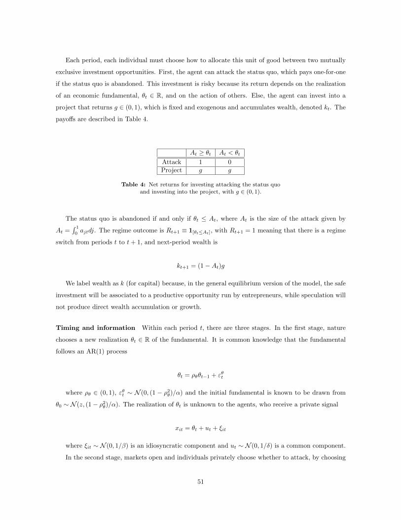
Each period, each individual must choose how to allocate this unit of good between two mutually

exclusive investment opportunities. First, the agent can attack the status quo, which pays one-for-one

if the status quo is abandoned. This investment is risky because its return depends on the realization

of an economic fundamental, ✓t

2 R, and on the action of others. Else, the agent can invest into a

project that returns g 2 (0, 1), which is fixed and exogenous and accumulates wealth, denoted k

t

. The

payo↵s are described in Table 4.

A

t

� ✓

t

A

t

< ✓

t

Attack 1 0Project g g

Table 4: Net returns for investing attacking the status quo

and investing into the project, with g 2 (0, 1).

The status quo is abandoned if and only if ✓t

A

t

, where A

t

is the size of the attack given by

A

t

=R 10 a

jt

dj. The regime outcome is Rt+1 ⌘ 1[✓

t

A

t

], with R

t+1 = 1 meaning that there is a regime

switch from periods t to t+ 1, and next-period wealth is

k

t+1 = (1�A

t

)g

We label wealth as k (for capital) because, in the general equilibrium version of the model, the safe

investment will be associated to a productive opportunity run by entrepreneurs, while speculation will

not produce direct wealth accumulation or growth.

Timing and information Within each period t, there are three stages. In the first stage, nature

chooses a new realization ✓t

2 R of the fundamental. It is common knowledge that the fundamental

follows an AR(1) process

✓

t

= ⇢

✓

✓

t�1 + "

✓

t

where ⇢✓

2 (0, 1), "✓t

⇠ N (0, (1 � ⇢

2✓

)/↵) and the initial fundamental is known to be drawn from

✓0 ⇠ N (z, (1� ⇢

2✓

)/↵). The realization of ✓t

is unknown to the agents, who receive a private signal

x

it

= ✓

t

+ u

t

+ ⇠

it

where ⇠it

⇠ N (0, 1/�) is an idiosyncratic component and u

t

⇠ N (0, 1/�) is a common component.

In the second stage, markets open and individuals privately choose whether to attack, by choosing

51

a(Iit

) 2 {0, 1}, or refrain and invest, k(Iit

) = 1� a(Iit

), where Iit

denotes agent i’s information set at

date t. In the third stage, At

is revealed publicly (although ✓t

remains unknown) and the status quo

is abandoned if and only if ✓t

A

t

. Note that the fact that A

t

is revealed at the end of the period

means that all within-period heterogeneity is wiped out and only the component yt

⌘ ✓

t

+ u

t

.

We suppose that no agent can observe the individual action of others (so that o↵-equilibrium

beliefs are not relevant). At period t, the information set of any agent i 2 [0, 1] is therefore Iit

=

{xt

i

, a

t�1i

, k

t�1i

;At�1}, where superscripts denote histories. Since all relevant information is made

public at the end of the period (in particular, agents do not use their private signals to update because

these become uninformative after the revelation of At

), the period-t individual posterior beliefs can be

summarized by common beliefs :

✓

t

|Iit

⇠ N�µ

t

, �

�1t

�

for all i 2 [0, 1]. This means that all relevant information can be summarized by the single state

vector (µt

, �

t

) at the beginning of period t+ 1.

Therefore, the law of motion for common beliefs is

µ

t+1 = ⇢

✓

�

t

µ

t

+ �y

t

�

t

+ �

�

t+1 =

✓⇢

2✓

�

t

+ �

+1� ⇢

2✓

↵

◆�1

for all t = 1, 2, . . . , with µ0 = ⇢

✓

z and �0 = ↵/(1�⇢2✓

) as the initial state vector. Note that posterior

mean and precision are common across agents (no need to keep track of the belief distribution) and

su�cient statistics for beliefs.

Equilibrium Adopting the convention that agents attack in case of indi↵erence, the optimal bidding

strategy at period t is

a(µt

, �

t

) =

8><

>:

1 if p(µt

, �

t

) � g

0 if p(µt

, �

t

) < g

where p(µt

, �

t

) is the posterior belief of a regime switch (thus also the expected payo↵ for attacking),

and the optimal investment strategy is k(µt

, �

t

) = 1� a(µt

, �

t

).

Conjecture that the model can be solved by monotone strategies. Then, there exist cuto↵ points

✓

⇤t

⌘ ✓

⇤(µt

, �

t

) and x

⇤t

⌘ x

⇤(µt

, �

t

) such that the status quo is abandoned if and only if ✓t

✓

⇤t

, and

an agent attacks if and only if her private signal satisfies xt

x

⇤t

, and otherwise invests in the project.

52

Since ✓t

|µt

, �

t

⇠ N (µt

, �

�1t

), the latter implies that we can write the posterior belief of a regime switch

as

p(µt

, �

t

) = P[✓t

✓

⇤t

|µt

, �

t

] = �⇣p

�

t

�✓

⇤t

� µ

t

�⌘

Since x

t

= ✓

t

+ u

t

+ ⇠

t

, then x

t

|✓t

⇠ N (✓t

,�

�1 + �

�1), and therefore the size of the attack is given

by

A(✓t

) = P[xt

x

⇤t

|✓t

] = �

s��

� + �

(x⇤t

� ✓

t

)

!

and �(✓t

) ⌘ 1�A(✓t

) is the fraction of agents who invest into the project at time t. The threshold

level ✓⇤t

that determines a regime switch solves ✓⇤t

= A(✓⇤t

), that is

✓

⇤t

= �

s��

� + �

(x⇤t

� ✓

⇤t

)

!(13)

Finally, the indi↵erence condition for the marginal trader says that p(µt

, �

t

) = g, or

�⇣p

�

t

�✓

⇤t

� µ

t

�⌘= g (14)

and the thresholds (x⇤t

, ✓

⇤t

) are defined as the unique joint solution to (13) and (14), given the state

(µt

, �

t

).

Figure 7 is an example of a simulated economy. The calibration is g = 0.5, ↵ = 1, � = 5, � = 20,

⇢

✓

= 0.98 and z = 0.5, for T = 100 periods. Note that, over time, At

converges toward zero and thus

k

t

does toward g. Intuitively, as time goes by, agents learn about ✓t

and coordinate into the safe and

“productive” investment. However, in the transit to this steady state, failures in coordination may

occur which may lead to sustained episodes of repeated attacks and extended economic cycles.

4.2 A dynamic general-equilibrium model of coordination-driven growth

The last subsection has proposed a preliminary example to show through simulation a simple mech-

anism that hints that episodes of sustained coordination can survive over and above fundamentally-

driven cycles of wealth. Admittedly, this point has been made with an extremely stylized partial-

equilibrium dynamic model of regime change. In this subsection I outline a general-equilibrium coun-

terpart of the same economy and present a definition for its equilibrium.

Demographics and production Time is discrete, runs forever and is indexed by t = 1, 2, . . . . There

is a measure-one continuum of infinitely-lived agents, indexed by i 2 [0, 1], and a single consumption

53

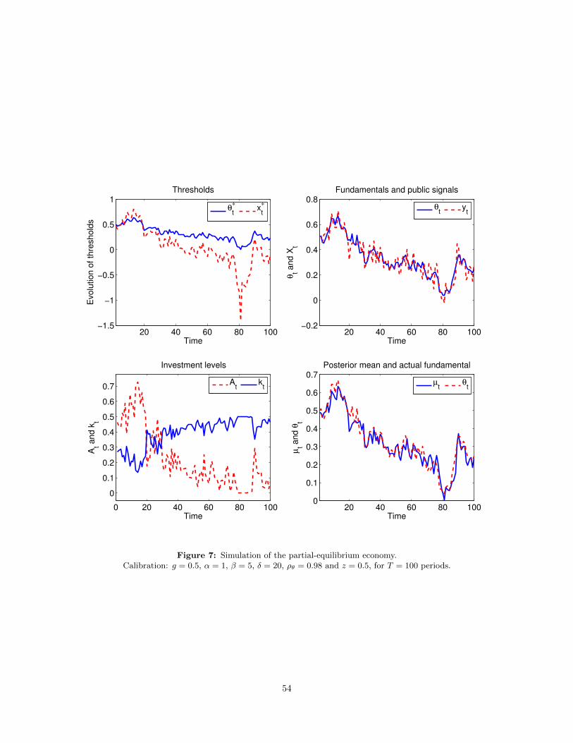
20 40 60 80 100−1.5

−1

−0.5

0

0.5

1Thresholds

Time

Evo

lutio

n o

f th

resh

old

s

θt∗ x

t∗

20 40 60 80 100−0.2

0

0.2

0.4

0.6

0.8

Time

θt a

nd

Xt

Fundamentals and public signals

θt

yt

0 20 40 60 80 100

0

0.1

0.2

0.3

0.4

0.5

0.6

0.7

Time

At a

nd k

t

Investment levels

At

kt

20 40 60 80 1000

0.1

0.2

0.3

0.4

0.5

0.6

0.7

Time

µt a

nd θ

t

Posterior mean and actual fundamental

µt

θt

Figure 7: Simulation of the partial-equilibrium economy.

Calibration: g = 0.5, ↵ = 1, � = 5, � = 20, ⇢✓

= 0.98 and z = 0.5, for T = 100 periods.

54

good (with unit price) produced with a constant-returns-to-scale production function Y

t

= F (Kt

, L

t

),

where Kt

2 R+ is the capital stock of the economy and L

t

2 [0, 1] is hours of labor, with K0 given and

nonnegative. Labor is supplied inelastically, or L

t

= 1, so that we can write production in intensive

form as Y

t

/L

t

= f(kt

), where f(kt

) ⌘ F (kt

, 1) and k

t

⌘ K

t

/L

t

. We assume that f

0(·) > 0 > f

00(·),

and the standard Inada conditions hold. Factor markets are competitive.

Investment opportunities In order to consume, each individual must allocate his wealth (i.e, wage

plus the returns on past investments) into either one of two investment technologies.

1. First, an individual can become a speculator. Turning into a speculator means choosing an

action a

it

2 {0, 1} within a Morris and Shin game, that is, investing into a project that pays o↵

one-for-one only if a su�ciently large fraction of agents undertake it. This is risky in the sense

that it pays o↵ depending on the action chosen by others, and pays more in expected terms the

more people undertake it (a payo↵ complementarity). This does not accumulate wealth for the

economy: the wage is stored at zero net return for next period.

2. Else, the individual can become an entrepreneur. Turning into an entrepreneur means investing

into a project that will turn into capital next period. This is a safe investment in the sense

that its outcome does not depend directly on the action of other entrepreneurs. The investment

technology is described by a function g(.), in the sense that investing w units of the good returns

g(w) units of capital, where g

0(·) > 0 > g

00(·). This capital is then rented out to the firm at a

rental rate of Rk.

As usual, the status quo is dropped in period t if ✓t

A

t

, and we let ⇡t+1 ⌘ 1[✓

t

A

t

] be the regime

outcome, with ⇡t+1 = 1 meaning that there is a regime switch from period t to t+1. Table 5 describes

the payo↵s.

A

t

� ✓

t

A

t

< ✓

t

Speculator 1 0Entrepreneur R

k

g(w) R

k

g(w)

Table 5: Net returns for investing attacking the status quo

and investing w into the capital-accumulation technology.

The law of motion of per-capita capital is

k

t+1 = �

t

g(wt

) + (1� �

k

)kt

(15)

55

where �k

2 [0, 1] is the depreciation rate of capital and �t

2 [0, 1] is the equilibrium mass of agents

who invest into capital (that is, the measure of speculators in the economy).

Equation (15) describes the growth pattern of the economy, and for now it is enough to note

that fluctuations in aggregate activity stem from two di↵erent sources: exogenously through capital

depreciation, and endogenously through changes in �t

(the extensive margin of investment).

Timing and information Timing and information are identical to the partial-equilibrium version

of the model. At each period t, it is common knowledge that the fundamental evolves according to an

auto-regressive process

✓

t

= ⇢

✓

✓

t�1 + "

✓

t

where ⇢✓

2 (0, 1), "✓t

⇠ N (0, (1 � ⇢

2✓

)/↵) and the initial fundamental level is known to be drawn

from ✓0 ⇠ N (z, (1 � ⇢

2✓

)/↵). The realization ✓t

is unknown throughout period t and at any point in

the future.

Within each period, there are three stages. In the first stage, nature draws ✓t

and each consumer

i observes an unbiased private signal xit

on it, given by:

x

it

= ✓

t

+ u

t

+ ⇠

it

where ⇠it

⇠ N (0, 1/�) and u

t

⇠ N (0, 1/�). In the second stage, all markets open, individuals

choose whether to become speculators or entrepreneurs, and each type of agent submits demands for

non-capital and capital investments, respectively, all of which are placed privately24. In the third

stage, At

is revealed publicly (so that y

t

⌘ ✓

t

+ u

t

serves as a public signal for the agents) and the

status quo is abandoned if At

� ✓

t

. Payments for both investment technologies are realized only at

the beginning of the next period.

Once again, posterior beliefs are common by the end of the period, such that ✓t

|xt

⇠ N (µt

, �

�1t

),

where posterior mean and precision evolve according to:

µ

t+1 ⌘ ⇢

✓

�

t

µ

t

+ �y

t

�

t

+ �

�

t+1 ⌘✓

⇢

2✓

�

t

+ �

+1� ⇢

2✓

↵

◆�1

for all t = 1, 2, . . . , with µ0 = ⇢

✓

z and �0 = ↵/(1� ⇢

2✓

). .

24Once more, the fact that individual actions are not observable by others allows us to ignore the role of o↵-equilibriumbeliefs.

56

Definition of a recursive equilibrium Each period t, an agent i with wage w

it

� 0 must decide

whether to become a speculator or an entrepreneur.

Let V

S(µ, �, k) be the value of becoming a speculator and V

E(µ, �, k) the value of becoming an

entrepreneur for an agent that starts a period with a belief system (µ, �) and the prevailing capital

stock is k. In each period, given beliefs about the fundamental, an agent can either invest in capital

or choose whether or not to attack the status quo.

The following defines a recursive equilibrium:

Definition 6 A symmetric monotone recursive PBE are value functions V (µ, �, k), V E(µ, �, k) and

V

S(µ, �, k) for the agent, the entrepreneur and the speculator, respectively; policy rules z(µ, �, k) � 0

and a(µ, �, k) 2 {0, 1}; factor prices R

k(k) and w(k) of capital and labor; measures A(k) 2 [0, 1] and

�(k) 2 [0, 1] of speculators and entrepreneurs; a perceived probability of regime switch P (✓; k) 2 [0, 1];

and a cdf (✓|µ, �, k) 2 [0, 1], such that, for any state (µ, �, k),

1. Consumers’ optimality: Given prices R

k(k) and w(k), the value function satisfies

V (µ, �, k) = max

⇢V

S(µ, �, k), V E(µ, �, k)

�

where

V

S(µ, �, k) = maxa

02{0,1}a

0✓Z +1

�1P (✓; k)d (✓|µ, �, k)

◆+ ⇢E

µ

0,�

0

V (µ0

, �

0, k

0)

����µ, �, k�

and

V

E(µ, �, k) = maxz

02�(k)R

k(k)g(z0) + ⇢Eµ

0,�

0⇥V (µ0

, �

0, k

0)��µ, �, k

⇤

�(k) ⌘�z

0 : 0 z

0 w(k) +R

k(k)g(z(µ, �, k)) + 1[A(✓,k)>✓]a(µ, �, k)

where ⇢ 2 (0, 1) is the time discount factor, and the Bellman equations have solutions at the

policy functions, namely a

0 = a(µ, �, k) and z

0 = z(µ, �, k).

2. Belief consistency: (✓|µ, �, k) is obtained by Bayes’ rule. In particular, ✓0|µ, � ⇠ N (µ, ��1),

with

µ

0 = ⇢

✓

�µ+ �y

� + �

�

0 =

✓⇢

2✓

� + �

+1� ⇢

2✓

↵

◆�1

The perceived probability of a regime switch is given by P (✓; k) = 1[A(✓,k)�✓], for each ✓ 2 R.

57

3. Equilibrium measures: The equilibrium measure of speculators is A(k) = ✓

?(k), where ✓?(k)

is the solution to the joint system for (x?(k), ✓?(k)):

✓

?(k) = �

s��

� + �

(x?(k)� ✓

?(k))

!

R

k(k)g(w(k)) = � (p�(✓?(k)� �))

The equilibrium measure of entrepreneurs is �(k) = 1�A(k).

4. Market clearing conditions: Competitive factor markets clear, so that w(k) = f(k)� kf

0(k)

and R

k(k) = f

0(k). Next-period capital is given by k

0 = �(k)g(w(k)) + (1� �

k

)k.

Note that, conditional on choosing to become a speculator, not attacking is never optimal, for a

weakly greater payo↵ could have been obtained by investing in capital as the continuation value is the

same in both cases. Therefore, all speculators attack the status quo. This is already imposed in the

definitions above, as A(✓, k) stands both for the aggregate size of the attack and the measure of agents

that become speculators.

Figure 8 is an example of a simulated economy. The calibration is f(kt

) = k

!

t

with ! = 0.3,

g(wt

) = w

#

t

with # = 0.3, ↵ = 3, � = 500, � = 50, �k

= 0.16, ⇢✓

= 0.99, k0 = 0.6 and z = R

k

0g(w0),

for T = 200 periods. Note that, over time, At

converges toward zero and thus k

t

does toward g.

Once again, in periods in which the fundamental is perceived to be low, there is coordination into

speculation, which lengthens the crisis in the real sector through a slower accumulation of capital.

My attention is now focused on the two models just outlined, which need to be made more tractable

and a little less stylized. This is very much work in progress.

5 Concluding remarks

This paper has surveyed theory and applications of the global games literature in macroeconomic

problems. The main justification for the use of this theory is in problems of coordination, in which

the commonality of certain payo↵-relevant information may lead to multiplicity of equilibria. We have

analyzed how the global games approach can select one such equilibrium within a particular class of

monotone strategy Bayesian-Nash equilibria. The main insights are not robust to the introduction of

public information, but it is still possible to derive uniqueness results for a large class of models that

allow us to draw determinate policy implications.

58

50 100 150 200

0.35

0.4

0.45

0.5

0.55

0.6

0.65

0.7Factor prices

Time

Fact

or

price

s

wt

Rtk

50 100 150 2000

0.1

0.2

0.3

0.4

0.5

Time

θt,

y t and

µt

Fundamentals, public signals and beliefs

θt

yt

µt

50 100 150 200

0

0.2

0.4

0.6

0.8

1

Time

At,

χt

Equilibrium measures

At

χt

50 100 150 2000.65

0.7

0.75

0.8

0.85

0.9

0.95

1

Time

f(k t)

and k

t

Investment and production

f(kt) k

t

Figure 8: Simulation of the general-equilibrium economy. Calibration: f(kt

) = k!

t

with ! = 0.3, g(wt

) = w#

t

with # = 0.3, ↵ = 3, � = 500, � = 50, �k

= 0.16, ⇢✓

= 0.99, k0 = 0.6 and z = Rk

0g(w0), for T = 200 periods.

59

References

[1] Angeletos, G.-M., and J. La’O (2013): “Sentiments,” Econometrica, 81(2), 739 – 779.

[2] Angeletos, G.-M., C. Hellwig, and A. Pavan (2006): “Signaling in a Global Game: Coordi-

nation and Policy Traps,” Journal of Political Economy, 114(3), 452 – 484.

[3] Angeletos, G.-M., C. Hellwig, and A. Pavan (2007): “Dynamic Global Games of Regime

Change: Learning, Multiplicity, and the Timing of Attacks,” Econometrica, 75(3), 711 – 756.

[4] Angeletos, G.-M., and I. Werning (2006): “Crises and Prices: Information Aggregation,

Multiplicity, and Volatility,” American Economic Review, 96(5), 1720 – 1736.

[5] Atkeson, A (2000): “Rethinking Multiple Equilibria in Macroeconomic Modeling: Comment,”

NBER Macroeconomics Annual, 15, 162 – 171.

[6] Banerjee, A.V. (1992): “A Simple Model of Herd Behavior,” The Quarterly Journal of Eco-

nomics, 107 (3), 797 – 817.

[7] Barlevy, G., and P. Veronesi (2003): “Rational Panics and Stock Market Crashes,” Journal

of Economic Theory, 110, 234 – 263.

[8] Bikhchandani, S., Hirshleifer, D., and I. Welch (1992): “A Theory of Fads, Fashion,

Custom, and Cultural Change as Informational Cascades,” Journal of Political Economy, 100 (5),

992 – 1026.

[9] Bloom, N. (2008): “The Impact of Uncertainty Shocks,” Econometrica, 77, 623 – 685.

[10] Broner, F. (2008): “Discrete Devaluations and Multiple Equilibria in a First Generation Model

of Currency Crises,” Journal of Monetary Economics, 55, 592 – 605.

[11] Burdzy, K., D.M. Frankel and A. Pauzner (2001): “Fast Equilibrium Selection by Rational

Players Living in a Changing World,” Econometrica, 69(1), 163 – 189.

[12] Calvo, G. A. (1988): “Servicing the Public Debt: The Role of Expectations,” American Eco-

nomic Review, 78, 647 – 661.

[13] Carlsson, H., and E. van Damme (1993): “Global Games and Equilibrium Selection,” Econo-

metrica, 61(5), 989 – 1018.

[14] Chamley, C. (1999): “Coordinating Regime Switches,” Quarterly Journal of Economics, 114,

869 – 905.

60

[15] Chamley, C. (2003): “Dynamic Speculative Attacks,” American Economic Review, 93, 603 –

621.

[16] Chari, V.V., and P. Kehoe (2003): “Hot Money,” Journal of Political Economy, 111(6), 1262

– 1292.

[17] Chassang, S. (2010): “Fear of Misscoordination and the Robustness of Cooperation in Dynamic

Global Games with Exit,” Econometrica, 78(3), 973 – 1006.

[18] Cole, H.L., and T. Kehoe (2000): “Self-Fulfilling Debt Crises,” The Review of Economic

Studies, 67(1), 91 – 116.

[19] Corsetti, G., A. Dasgupta, S. Morris, and H.S. Shin (2004): “Does One Soros Make

a Di↵erence? A Theory of Currency Crises with Large and Small Traders,” Review of Economic

Theory, 71, 87 – 113.

[20] Corsetti, G., B. Guimaraes, and N. Roubini (2006): “International Lending of Last Resort

and Moral Hazard: A Model of IMF’s Catalytic Finance,” Journal of Monetary Economics, 53 (3),

441 – 471.

[21] Dasgupta, A. (2007): “Coordination and Delay in Global Games,” Journal of Economic Theory,

134 (1), 195 – 225.

[22] Diamond, P. (1982): “Aggregate Demand Management in Search Equilibrium,” Journal of Po-

litical Economy, 90, 881 – 894.

[23] Edmond, C. (2013): “Information Manipulation, Coordination and Regime Change,” Review of

Economic Studies, 80 (4), 1422 – 1458.

[24] Diamond, D., and P. Dybvig (1983): “Bank Runs, Deposit Insurance, and Liquidity,” Journal

of Political Economy, 91, 401 – 419.

[25] Fajgelbaum, P., E. Schaal, and M. Taschereau-Dumouchel (2014): “Uncertainty Traps,”

National Bureau of Economic Research, working paper no. 19973.

[26] Frankel, D.M., and A. Pauzner (2000): “Resolving Indeterminacy in Dynamic Settings: The

Role of Shocks,” Quarterly Journal of Economics, 115(1), 285 – 304.

[27] Flood, R., and P. Garber (1984): “Collapsing Exchange-rate Regimes: Some Linear Exam-

ples,” Journal of International Economics, 17, 1 – 13.

[28] Ginnitsarou, G., and F. Toxvaerd (2012): “Recursive Global Games,” University of Cam-

bridge and CEPR, working paper.

61

[29] Goldstein, I., and A. Pauzner (2005): “Demand-Deposit Contract and the Probability of

Bank Runs,” The Journal of Finance, 60(3), 1293 – 1326.

[30] Goldstein, I., E. Ozdenoren, and K. Yuan (2011): “Learning and Complementarities in

Speculative Attacks,” Review of Economic Studies, 78, 263 – 292.

[31] Grossman, S.J., and J. Stiglitz (1980): “On the Impossibility of Informationally E�cient

Markets,” American Economic Review, 70(3), 393 – 408.

[32] Hellwig, C. (2002): “Public Information, Private Information, and the Multiplicity of Equilibria

in Coordination Games,” Journal of Economic Theory, 107, 191 – 222.

[33] Hellwig, C., and L. Veldkamp (2008): “Knowing What Others Know: Coordination Motives

in Information Acquisition,” The Review of Economic Studies, 76, 223 – 251.

[34] Hellwig, C., A. Mukherji, and A. Tsyvinski (2006): “Self-Fulfilling Currency Crises: The

Role of Interest Rates,” American Economic Review, 96(5), 1769 – 1787.

[35] Krugman, P. (1979): “A Model of Balance-of-Payments Crises,” Journal of Money, Credit, and

Banking, 11(3), 311 – 325.

[36] Levin, J. (2000): “Collective Reputation,” Stanford University, working paper.

[37] Levin, J. (2001): “A Note on Global Games with Overlapping Generations,” Stanford University,

working paper.

[38] Lucas, R. E. (1975): “An Equilibrium Model of the Business Cycle,” Journal of Political Econ-

omy, 83, 1113 – 1144.

[39] Mathevet, L., and J. Steiner (2013): “Tractable Dynamic Global Games and Applications,”

Journal of Economic Theory, 148, 2583 – 2619.

[40] Matsui, A. (1999): “Multiple Investors and Currency Crises,” University of Tokyo, working

paper.

[41] Morris, S., and H.S. Shin (1998): “Unique Equilibrium in a Model of Self-Fulfilling Currency

Attacks,” American Economic Review, 88(3), 587 – 597.

[42] Morris, S., and H.S. Shin (1999): “A Theory of the Onset of Currency Attacks,” Asian

Financial Crisis: Causes, Contagion and Consequences, ed. P.-R. Agenor, D. Vines and A. Weber,

230 – 261. Cambridge: Cambridge University Press.

62

[43] Morris, S., and H.S. Shin (2002): “Social Value of Public Information,” American Economic

Review, 92(5), 1521 – 1534.

[44] Morris, S., and H.S. Shin (2003): “Global Games: Theory and Applications,” Advances in

Economics and Econometrics: Theory and Applications, Eighth World Congress, ed. Mathias De-

watripont, Lars P. Hansen, and Stephen J. Turnovsky, 56 – 114. Cambridge: Cambridge University

Press.

[45] Morris, S., and H.S. Shin (2004): “Coordination Risk and the Price of Debt,” European

Economic Review, 48(1), 133 – 153.

[46] Muth, J. F. (1961): “Rational Expectations and the Theory of Price Movements,” Econometrica,

29, 315 – 335.

[47] Obstfeld, M. (1986): “Rational and Self-Fulfilling Balance-of-Payments Crises,” American Eco-

nomic Review, 76(1), 72 – 81.

[48] Obstfeld, M. (1996): “Models of Currency Crises with Self-Fulfilling Features,” European Eco-

nomic Review, 40(3–5), 1037 – 1047.

[49] Oyama, D. (2004): “Booms and Slumps in a Game of Sequential Investment with the Changing

Fundamentals,” Japanese Economic Review, 55, 311 – 320.

[50] Rochet, J.-C., and X. Vives (2004): “Coordination Failures and the Lender of Last Resort:

Was Bagehot Right after All?,” Journal of European Economic Association, 6, 1116 – 1147.

[51] Sargent, T. J. (1991): “Equilibrium with Signal Extraction from Endogenous Variables,” Jour-

nal of Economic Dynamics and Control, 15, 245 – 273.

[52] Steiner, J. (2008): “Coordination cycles,” Games and Economic Behavior, 63(1), 308 – 327.

[53] Townsend, R.M. (1983): “Forecasting the Forecast of Others,” Journal of Political Economy,

91(4), 546 – 588.

63