Global Dynamics in Macroeconomics:

An Overlapping Generations Example�

Pere Gomis-Porqueras

Economics Department

University of Texas at Austin

�Alex Haro

Departament de Matem�atica Aplicada

Universitat de Barcelona

Abstract

In this paper we present two techniques used in the dynamical systems literature that

let us compute the shape of the stable and unstable manifolds of a given dynamical

system. These techniques can be used to study how an economy behaves as it moves

far away from the steady state. As a result, we can quantify the di�erence between

a local and a global analysis. In order to illustrate these techniques, we present a

general equilibrium model under two di�erent policy regimes demonstrating that the

local and global dynamics of an economic system can be substantially di�erent.

1 Introduction

In the early seventies Smale raised some concerns regarding the static nature of the equi-

librium concept resulting from Debreu's Theory of Value [5]. The theory did not attempt

�The authors would like to thank David Kendrick, Wolfgang Keller, Chris Sleet and Rafael de la Llave

for their helpful comments and insightful discussions. The authors would also like to thank the partcipants

of the Working Seminar on Dynamical System Series at the University of Texas at Austin for their valu-

able comments. The source code can be obtained upon request by writing to haro@math.utexas.edu or

gomis@eco.utexas.edu.

1

to answer the question \how is equilibrium reached?" Instead, dynamic considerations

were necessary to resolve this question. As Smale said \sometimes static theories pose

paradoxes whose resolution lies in a dynamic perspective" [14]. In particular, the study of

macroeconomics can not be completely understood without the use of a dynamic process.

Many macroeconomic concepts rely on intertemporal trade o�s, thus inherently embracing

the concepts and methodology of dynamical systems. Therefore, many of the phenomena

that macroeconomists study intrinsically involve a dynamic process. As Costas Azariadis

points out, \macroeconomics is about human interactions over time" [2].

In the representative agent framework we often encounter problems where it is impos-

sible to attain closed form solutions while iterating the Bellman equation. As a result we

need to resort to numerical methods to characterize the equilibria. The approximations

used to solve these problems tend to be local, although there is an increasing interest in

nonlocal approximations. In this spirit, Gaspar and Judd (1997) address the problem of

computing equilibria of large rational expectations models that go beyond the standard

linearization method which uses perturbation and projection methods to multidimensional

dynamic models. Gaspar et al (1997) show that rational expectation models of moderate

size can be quickly solved using nonlocal approximation methods. Their research hints

that computationally speaking the dominant approach to large models with Euler equation

formulations will be �xed-point iteration solution methods combined with complete poly-

nomial bases. The authors suggest that these techniques will outperform Newton-based

methods and monotone- and contraction-operator methods [8]. As they argue, \future

work should examine the quality of the approximation in various speci�c contexts, in par-

ticular competitive equilibria". In the same spirit, Guu and Judd (1997) show the gain of

a Taylor series expansion approach while studying the global properties in an aggregate

growth model [9]. Finally, there is an increasing number of articles that address the im-

portance of complex dynamics and global analysis in non representative agent frameworks.

For example, Yokoo (2000) investigates the global dynamics using a perturbation method

identifying conditions under which homoclinic points to the golden rule are generated with

an overlapping generations model [16]. Similarly, Bischi, Gardini and Kopel (2000) analyze

global bifurcations in a marketing model of market share attraction [3].

The purpose of this paper is similar in spirit to Gaspar and Judd (1997) and Guu

and Judd (1997). In this paper we characterize the dynamic behavior of a particular

economy as it moves away from the steady state. We treat the dynamical system as given

2

as is the case in most overlapping generation models. In order to investigate the global

dynamics of an economy, we introduce some mathematical techniques used in the dynamical

systems literature. We explore global properties of a dynamical system using successive

local approximations.1

2 Importance of global dynamics in macroeconomics

The pioneering modern macroeconomic models tended to be one dimensional systems.

Nowadays, many macroeconomic models are described by multidimensional systems. In

the one dimensional world the phase diagram can describe the most important aspects of

any dynamical system.2 Once we move away from the one dimensional world the study

of global dynamics becomes more complicated. For instance, higher dimensional systems

have the possibility of both expansion and contraction of the same invariant set, which

gives rise to new nonstationary equilibria.

A �rst step towards a better understanding of the global behavior of a given macroeco-

nomic system or, in general, a dynamical system, is to identify its invariant objects, such as

�xed points, periodic orbits or their associated invariant manifolds. The steady states of an

economic system are interpreted as descriptions of the long run behavior of the economy;

i.e, the �xed points of the dynamical system or if there are uctuations, the corresponding

periodic orbits. But if one wants to study the transition dynamics of the economy, one

needs to characterize how the dynamical system evolves through time. One may classify

these steady states by studying the temporal evolution of a point that is near the steady

state; i.e, its stability. In particular, we can classify a steady state as stable if all orbits that

start near it stay near it, and asymptotically stable if all orbits that start near it converge

to the �xed point. On the other hand, we classify a steady state as unstable if all orbits

that start near it move away from it. Finally, as we move from the one dimensional world

a new type of stability arises, saddle path stability. In this situation an orbit that starts

near the steady state stays near it only for a given subset of initial conditions.3 With this

classi�cation in mind, one can then describe the short run e�ect of di�erent policy regimes.

1This methodology is similar to Judd's perturbation and projection methods.2A classic example in macroeconomics is Solow's (1956) unidimensional law of motion for capital accu-

mulation. We note that even with one dimensional systems, one can �nd very complicated dynamics. A

classic example of complex behavior is the logistic map which can give rise to cycles of any period.3This latter type of situation is the most frequent in economics.

3

Among the invariant objects, the invariant manifolds of codimension 1 are very impor-

tant because they split the phase space into non connected regions. The standard practice

in economics is to consider the linear approximations of these manifolds.4 But when we

contemplate the nonlinear properties of these manifolds their associated non connected

regions can behave quite di�erently. For example, when we consider global properties we

may �nd transport phenomena and resonances. Furthermore, these non linear manifolds of

codimension 1 can also introduce barriers to the dynamical system. In other words, they

can impose some physical obstructions to the existence of invariant curves when studying

area preserving maps. It is therefore convenient to have fast computational methods that

enable us to study these non linear manifolds which may shed some light on some economic

puzzles.

Finally, there are several reasons why being able to describe the properties of a dynam-

ical system is of paramount interest. One of the most important is the fact that once we

determine the characteristics of the dynamical system, there is the possibility of controlling

the system. If economics was like physics, with its controlled experiments, one could, in

principle, choose preferred paths for the economy by setting appropriate controls and initial

conditions. Unfortunately, economics does not have as many degrees of freedom as in the

natural sciences.5 In particular, in the physical sciences one is able to chose the initial

conditions. In economics, on the other hand, the initial conditions are always given.

The fact that we can not choose initial conditions and the fact that most economists are

interested in how exogenous shocks are transmitted through the economy strongly suggests

the study of global dynamics. Furthermore, if shocks to the economy are suÆciently large

and the change in policies substantially alters the laws of motion of our economy, then a local

analysis may be somewhat uninformative. Lastly, the advantages of considering a global

analysis is that we can determine the quality of the local approximation. Furthermore, a

global analysis can also capture new dynamical phenomena not observed when performing

linear analysis. For instance, wandering cycles which can predict cyclic patterns of di�erent

periods, and homoclinic points which can yield chaotic behavior. These new phenomena

may be able to shed some light on some economic puzzles like the changing periodicity of

4These models investigate how the economy evolves as we perturb the economy slightly away from the

steady state. This local analysis can be considered as a �rst approximation to the dynamical problem.5In a world with multiple equilibria that can be Pareto ranked initial conditions become quite relevant.

In such a world, the policy maker, in principle, could pick initial conditions to rule out inferior equilibria.

4

business cycles or the di�erent rates of convergence.

3 Global analysis

In this section we present some mathematical techniques used in the dynamical systems

literature that enable us to study the behavior of a system away from the steady state.6

In particular, we primarily focus our attention on techniques that let us learn more about

the shape of the stable and unstable manifolds of a given dynamical system.

In order to clarify ideas, consider a generic dynamical system. The dynamical system

that we consider is a discrete planar system, which is given by the following smooth map

F = (f; g) : R � R ! R � R. The motion of this dynamical system is given by a sequence

of points Xt = (xt; yt) such that

0@ xt+1

yt+1

1A =

0@ f(xt; yt)

g(xt; yt)

1A : (1)

Once the steady states are determined, we can study how the system evolves through

time as we move away from the steady state. For convenience, we choose the coordinates

so that the steady state is at the origin. If our �xed point is hyperbolic, the corresponding

Jacobian matrix of the �xed point has no eigenvalue with modulus equal to one, then local

behavior around a hyperbolic �xed point is like the linearized system in terms of continuity

(but not di�erentiability necessarily), as asserted by the Hartman-Grobman theorem. In

many instances one can get di�erential or analytic equivalence using the normal forms

theorems of Poincare, Dulac and Siegel (see [1] or [11] for a detailed description of the

theorems).

We will further assume that the �xed point has real eigenvalues. One eigenvalue, �s, is

inside the unit circle and the other one, �u, is outside of it.7 The corresponding eigenvectors

for �s and �u are vs and vu respectively.

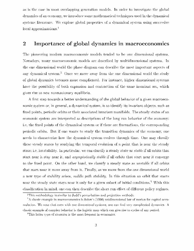
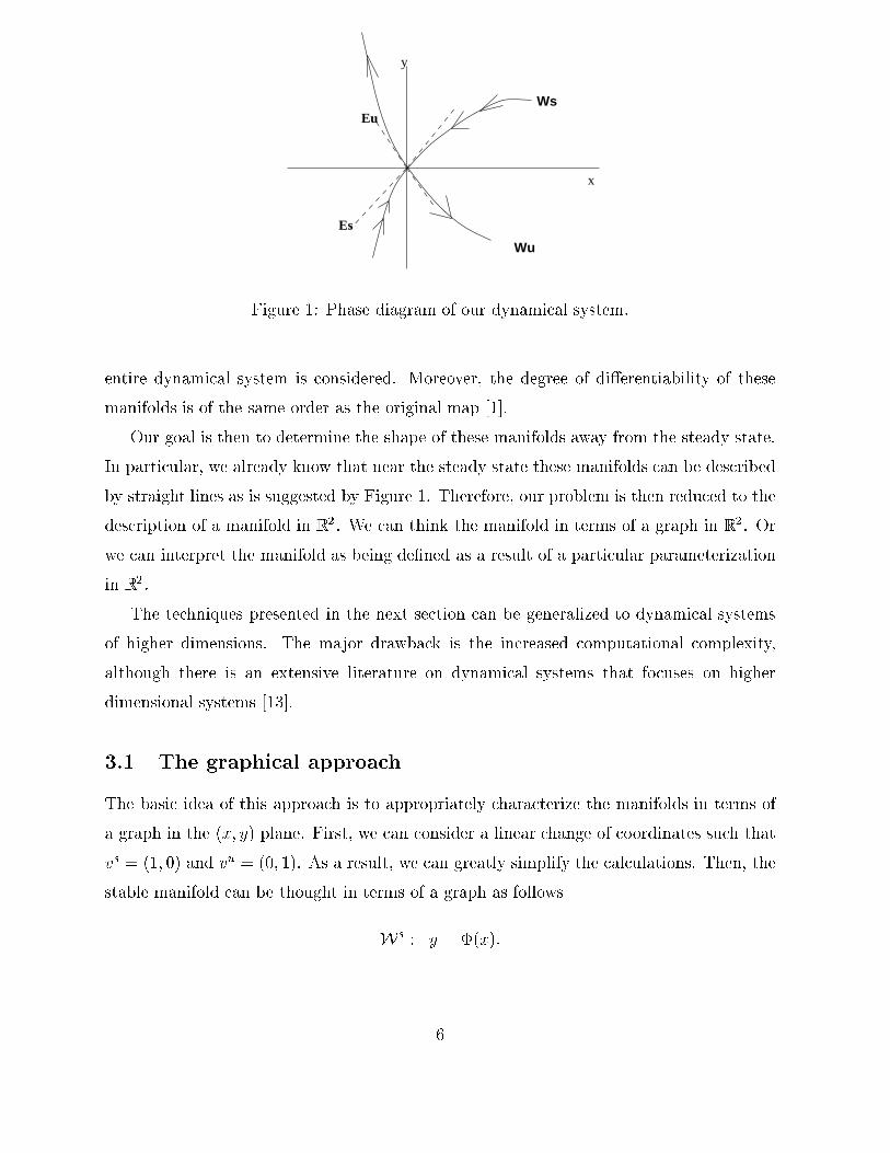
In order to clarify ideas let's assume that the phase diagram corresponding to the

dynamical system is described by Figure 1; where the linear stable and unstable subspaces

Es=<vs> and Eu=<vu> become the stable and unstable manifoldsWs andWu when the

6In the dynamical system literature, local analysis refers to a linear description of the system and global

analysis refers to a nonlinear description.7As is the case in most economic applications.

5

x

y

Ws

Wu

Eu

Es

Figure 1: Phase diagram of our dynamical system.

entire dynamical system is considered. Moreover, the degree of di�erentiability of these

manifolds is of the same order as the original map [1].

Our goal is then to determine the shape of these manifolds away from the steady state.

In particular, we already know that near the steady state these manifolds can be described

by straight lines as is suggested by Figure 1. Therefore, our problem is then reduced to the

description of a manifold in R2 . We can think the manifold in terms of a graph in R2 . Or

we can interpret the manifold as being de�ned as a result of a particular parameterization

in R2 .

The techniques presented in the next section can be generalized to dynamical systems

of higher dimensions. The major drawback is the increased computational complexity,

although there is an extensive literature on dynamical systems that focuses on higher

dimensional systems [13].

3.1 The graphical approach

The basic idea of this approach is to appropriately characterize the manifolds in terms of

a graph in the (x; y) plane. First, we can consider a linear change of coordinates such that

vs = (1; 0) and vu = (0; 1). As a result, we can greatly simplify the calculations. Then, the

stable manifold can be thought in terms of a graph as follows

Ws : y = �(x):

6

Similarly for the unstable manifold

Wu : x = (y):

Without loss of generality, we focus our attention on the construction of the stable man-

ifold. Since the stable manifold is tangent to the corresponding linear space at the steady

state, we know that the following conditions have to be veri�ed: �(0)=0 and �0(0)=0.8

Furthermore, since the stable manifold is invariant, any point on it moves to another point

on the manifold. In other words,

0@ x

y

1A =

0@ x

�(x)

1A �!

0@ f(x;�(x))

g(x;�(x))

1A : (2)

The resulting invariance equation for this dynamical system is then

g(x;�(x)) = �(f(x;�(x))): (3)

Notice that since x determines the position on the graph, the evolution of this variable

which is given by

x! f(x;�(x))

completely determines the dynamics on Ws.

In order to further characterize the global properties of the stable manifold, we Taylor

expand this unknown function, �(x), around the steady state (0; 0) which is given by

�(x) = �2x2 + �3x

3 + : : : ;

where the `: : :' represent terms of higher order.

We then perform a similar expansion for the dynamical system

f(x; y) = �sx + f2(x; y) + : : :

g(x; y) = �uy + g2(x; y) + : : : ;

where fk; gk are homogeneous polynomials of order k.9 Note that due to the initial linear

transformation the resulting Taylor expansion is greatly simpli�ed. From now on, we shall

use the notation f�k(x; y)=f2(x; y) + : : :+ fk(x; y) to denote a function up to order k.

8Note that if vs = (vsx; v

s

y) we need v

s

x6= 0 because �0(0)=

vs

y

vsx

.9A homogeneous quadratic polynomial is denoted by f2(x; y) = fxxx

2 + fxyxy + fyyy2.

7

In contrast to the known coeÆcients corresponding to the polynomials fk; gk describing

the dynamical system, we need to �nd the unknown coeÆcients �k corresponding to the

stable manifold. The main idea of this graphical approach is to �nd these unknown coef-

�cients by matching polynomials of the same order. Notice that we already know the �rst

two terms since �(0)=0 and �0(0)=0. In order to obtain the kth order term with k�2, we

impose the invariance condition up to order k. In other words, we need to compose the

di�erent functions, as suggested by equation (3), keeping track of the coeÆcients of the

same order and cutting o� the terms of order greater than k. We can then �nd closed form

solutions for these unknown coeÆcients, �k.10

Algebraically speaking, the calculation of these coeÆcients �k is as follows. Assuming

that the coeÆcients corresponding to �<k have already been computed, we describe a

recurrence method. In what follows the `: : :' represent terms of order higher that k. The

left hand side term of the invariance equation can then be written as follows:

g(x;�(x)) = �u��<k(x) + �kx

k�+ g�k(x;�<k(x)) + : : : ;

Similarly, we have the following expression for the right hand side term of the invariant

equation,

�(f(x;�(x)) = �<k(�sx + f<k(x;�<k)) + �k(�sx)k + : : : :

Thus, the kth coeÆcient that we need to solve for our invariance condition is given by the

following linear equation, the homology equation,

(�u � �ks)�kxk = (�<k(�sx + f<k(x;�<k)))�k � �u�<k(x)� (g�k(x;�<k(x)))�k

= ckxk:

Notice that the terms of order lower than k vanish because �<k satis�es the invariance

equation up to the order k-1. As a result, the only remaining term is ckxk. Therefore, we

can easily solve for �k which is given by

�k =ck

�u � �ks:

As we can see, whenever we have a saddle �xed point we can always compute all the

coeÆcients corresponding to the Taylor expansion of the manifold. Notice that this method

10This approach is similar in spirit to Judd's perturbation method [10].

8

can be generalized to other cases, although resonances may appear. Suppose, for instance,

that the two eigenvalues satisfy the following condition, 0<�f<�s< 1 where 'f' and 's' stand

for fast and slow, respectively.11 In this situation the �xed point is stable, attracting all

points in a neighbourhood around the steady state. When solving the homology equation

for the `fast' invariant manifold, �k(�s � �kf) = ck, we realize that �k is well de�ned 8k.

However, if we want to compute the `slow' invariant manifold a resonance may appear;

that is, there may exist a value of k such that �f=�ks . Under these circumstances, we can

not solve the homology equation as long as ck 6= 0. The `slow' manifold is dynamically

interesting because the dynamics around the �xed point collapses into it since the `fast'

component approaches the �xed point very rapidly. See Cabr�e et al (1999) for a detailed

description of this sort of phenomena [4].12

3.2 The parameterization approach

The basic goal of the parameterization approach is to describe the manifolds through an

appropriate parameterization in the (x; y) plane. In particular, for the stable manifold

we may chose the following parameterization W s: � ! (�) and the dynamics on the

manifold is given by � ! �s� . As we can see, this approach ensures that the iterated point

is just a \translation" on the manifold. In other words, we are �xing the dynamics on the

manifold.13

The resulting invariance equation is then given by the following expression

F ((�)) = (�s�); (4)

where we recall that F = (f; g) : R�R ! R�R with (0) = (0; 0). Now taking derivatives

on the both sides of the equation and setting � = 0, we have the following condition

DF (0; 0)D(0) = �sD(0);

where D(0) must be an eigenvector of the linearized system whose eigenvalue is �s.

In order to gather information about the global properties of the stable manifold we

proceed as in the previous case. In other words, we Taylor expand around the steady state

11Let vf and vs denote the corresponding eigenvectors.12This class of techniques has been recently used to study chemical processes and reactions [7].13This approach is similar in spirit to Judd's projection method [10].

9

(�) =

0@ x(�)

y(�)

1A =

0@ x1� + x2�

2 + : : :

y1� + y2�2 + : : : ;

1A = !1� + !2�

2 + : : : ;

keeping in mind that our goal is to �nd the unknown vectors !2, !3, : : :; where !1 = (vsx; vsy).

Let A=DF (0; 0) denote the linear part of our system. Suppose we already know

!2; : : : ; !k�1 and we want to obtain !k. The left-hand side of the invariance equation

up to order k is given by

F ((�)) = A (<k(�) + !k�k) + F�k(<k(�)) + : : :

Similarly for the right-hand side of the invariant equation,

(�s�) = <k(�s�) + !k�ks�

k + : : : :

Thus, the kth vector from the invariance condition, equation (4), can be represented by

the following linear equation

(A� �ksI)�k!k = <k(�s�)� A<k(�)� (F<=k(<k(�)))�k = zk�

k;

where zk is a known vector. We can easily solve this linear system and solve for !k, which

is given by

!k = (A� �ksI)�1zk:

As we saw earlier, if the �xed point is a saddle point we can not �nd resonances. This

technique can also be generalized to higher dimensions and other types of stability. Finally,

we may �nd resonances whenever det(A-�ksI) = 0.

3.3 Numerical considerations

In the previous sections we have examined two di�erent approaches to compute the man-

ifolds of a given dynamical system. We now explore the numerical advantages and disad-

vantages of their implementation. Since both methods rely on the invariant condition, we

can use this invariant property to �nd any possible programming errors. Note that at every

step k we can see if the computation is satisfactory because the invariance condition up to

order k-1 has to be satis�ed.14

14The kth order term gives rise to the homology equation.

10

There are some computational drawbacks that we need to consider. From a geometrical

point of view, the parametric approach seems to be more suitable. In principle, the graph-

ical approach can only be used when the underlying dynamical system yields well-behaved

manifolds, that is, they \do not bend backwards". This problem can be avoided, however,

by taking a small enough `fundamental' domain of the curve. We can then recover the

entire manifold by iterating this fundamental domain.

The Taylor expansions used in the previous sections give an approximation of the man-

ifold that is better than its linear approximation. But even in the analytic case, where

we can compute `all' the terms corresponding to a particular expansion, we may have a

�nite radius of convergence. For instance, the function y=1� 1

1+x2is well de�ned over the

real numbers, but its Taylor expansion around 0, y =x2 � x4 + x6 � : : :, is not de�ned

for jxj�1. As a result, the corresponding manifolds of the planar dynamical system may

not be de�ned 8 R2 , which should be taken into account when programming so we do not

consider these regions of our domain.

4 An example: An overlapping generations model

In this section we consider a monetary general equilibrium model under two di�erent policy

rules taken from Schreft and Smith (1997) [12]. This paper addresses the implications for

monetary policy when there is an exogenous decreasing demand for cash. The economy

consists of two identical islands with limited communication. These islands are inhabited by

an in�nite sequence of two period lived overlapping generations. Agents have an endowment

of the single nonstorable good when young and nothing when old. In addition, agents derive

utility from consumption only when old. To generate a demand for cash transactions,

the model incorporates spatial separation and limited communication along the lines of

Townsend (1987) [15]. To generate a role for banks, the model includes shocks to liquidity

needs resembling those in Diamond and Dybvig (1983) [6]. Furthermore, the underlying

assets in this economy are government-issued �at currency and government bonds. It is

assumed that �at money is dominated in the rate of return. Therefore, banks will hold

the minimum amount of cash possible so that they can meet the liquidity needs of their

depositors. These features imply a derived demand for base money that depends on the

need for currency in payments and the demand by banks for cash reserves.

With this environment in mind, we explore how the economy dynamically evolves under

11

di�erent policy rules, targeting in ation and having a constant money growth rate. Fur-

thermore, we compare the corresponding manifolds that one obtains using a local versus a

global approach.

4.1 Targeting in ation

Under this scenario the Central Bank targets the in ation rate. The dynamical system

corresponding to this policy rule is given by the following system of equations

P = (It � (It � 1) (It; �t)) (5)

�t+1 � �� = �(�t � ��) (6)

where It represents the gross nominal interest rate for bond holdings, �t denotes the fraction

of households that require cash in order to transact, �(<1) represents the speed at which

the money demand decreases, P is the targeted in ation rate and (It; �t) is the optimal

cash reserves held by banks. For this particular model, the optimal cash reserves is given

by

(It; �t) =1

1 + 1��t�t

I1��

�

t

(7)

where � is the coeÆcient of relative risk aversion.

As we can see, this dynamical system is a decoupled system; i.e, the dynamics of It

are inherited by the dynamic behavior of �t. Furthermore, since the dynamics of �t are

determined by a linear system, the local and global analysis are exactly the same. There-

fore, the local dynamics corresponding to this particular policy regime does not introduce

any approximation error nor new dynamical phenomena. As a result, the corresponding

manifold is just a straight line.

4.2 Constant money growth rate

Under this policy rule the Central Bank keeps printing �at money at a constant rate. In

other words,

Mt+1 = �Mt (8)

where Mt is the total money supply at time t and � is the constant money growth rate.

The dynamical system corresponding to this policy rule is given by the following system of

12

equations

It+1 =

��t+1

�(1� �t+1)

�1� �t

�tI

1

�

t � (� � 1)

�� �

1��

(9)

�t+1 � �� = �(�t � ��): (10)

The dynamics of the gross nominal interest rate are much more complicated than the

previuos example. The e�ect of a decreasing demand for money now in uences how the

nominal interest rate changes over time. As a result, we may �nd very di�erent local and

global dynamics.

4.2.1 A numerical example

In order to explore the di�erence between a local versus a global approach we numeri-

cally computed the shape of the manifolds. As a simpli�cation, we are going to consider

economies with �=0:5 in order to avoid rational exponents. As a result, we can compute as

many coeÆcients corresponding to the manifold as desired. The resulting economy evolves

as follows,

It+1 =�t+1

�(1� �t+1)

�1� �t

�tI2t � (� � 1)

�(11)

�t+1 � �� = �(�t � ��): (12)

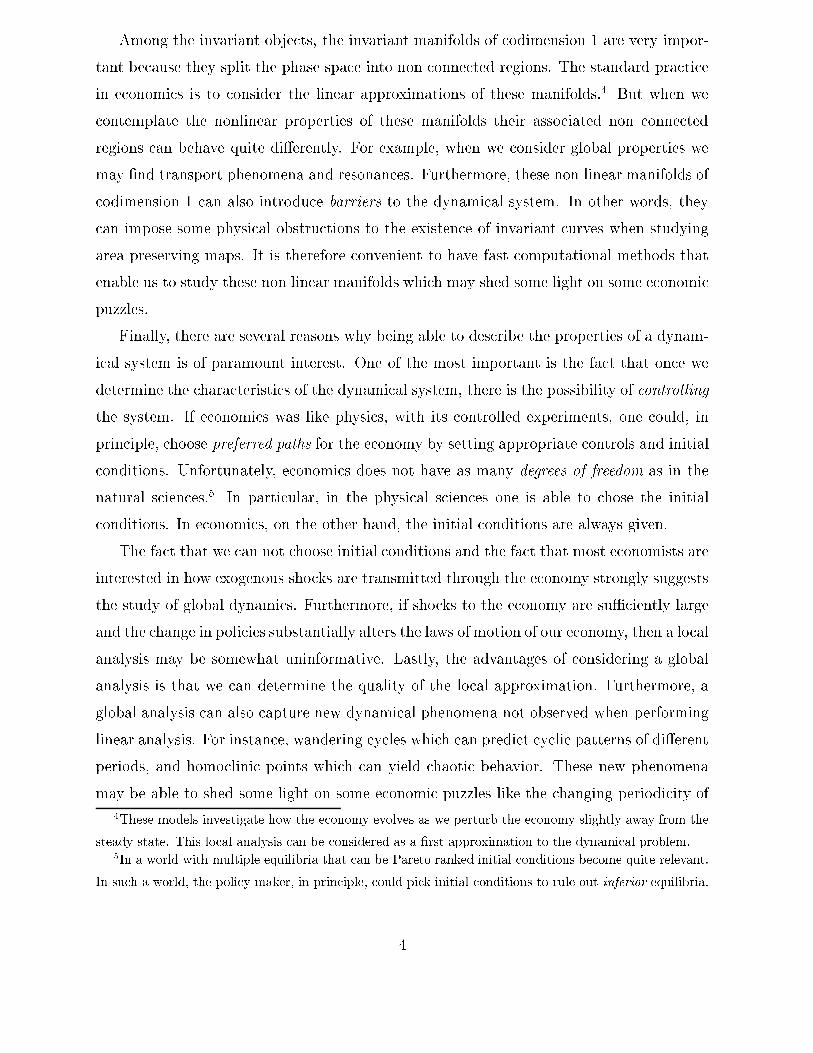
We next compute the stable and unstable manifolds corresponding to an economy with

the following properties �=0.8, �=1.1 and ��=0.2, see Figure 2.

As we can see, the stable and unstable manifolds do a better job of describing the

dynamics as we move farther away from the steady state than do their linear counterparts.

In this case, the linear unstable space coincides with the unstable manifold. On the other

hand, the linear stable space and the stable manifold are not the same. The stable manifold

is computed using the parameterization method up to order 50. The convergence radius of

the series is approximately 0:363.15

In order to emphasize the error associated with the local approximation, we have per-

formed two of numerical exercises. When studying the phase diagram of a planar system,

15Throughout our numerical exercise we used a Pentium III processor and the time required for our

program to compute all the manifolds was approximately one quarter of a second.

13

0.5 1 1.5

I

0

0.1

0.2

0.3

0.4

π

Wu

Ws

Es

Figure 2: The stable and unstable manifolds and their linear counterparts.

we divide the phase space into four regions. These regions then determine the trajectory

of a point if it were to fall into that region. In order to see how di�erent these trajectories

may be, we compute the image of the linear stable manifold. By doing so we can determine

how invariant the linear approximation really is, see Figure 3.

0.5 1 1.5

I

0

0.1

0.2

0.3

0.4

π

Wu

Ws

Es F(E

s)

Figure 3: The manifolds corresponding to �=0.5, �=0.8, �=1.1 and ��=0.2.

The trajectories corresponding to the linear manifold are di�erent from the nonlinear

manifold. As a result, we �nd that the predictions corresponding to the linear manifold can

be substantially misleading since they allow trajectories that are otherwise not possible.

We also consider how the dynamical system evolves as we increase the money growth

rate. As shown in Figure 4, the shape of the stable manifold becomes more linear near the

14

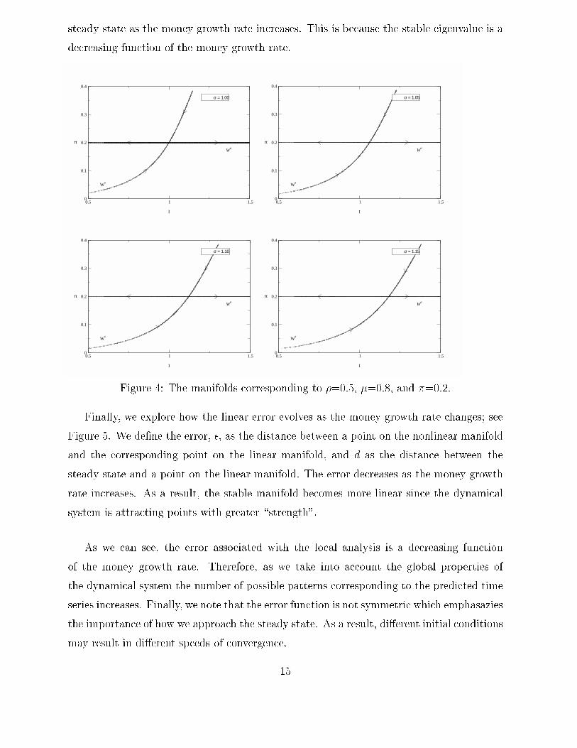
steady state as the money growth rate increases. This is because the stable eigenvalue is a

decreasing function of the money growth rate.

0.5 1 1.5

I

0

0.1

0.2

0.3

0.4

π

σ = 1.00

Wu

Ws

0.5 1 1.5

I

0

0.1

0.2

0.3

0.4

π

σ = 1.05

Wu

Ws

0.5 1 1.5

I

0

0.1

0.2

0.3

0.4

π

σ = 1.10

Wu

Ws

0.5 1 1.5

I

0

0.1

0.2

0.3

0.4

π

σ = 1.15

Wu

Ws

Figure 4: The manifolds corresponding to �=0.5, �=0.8, and ��=0.2.

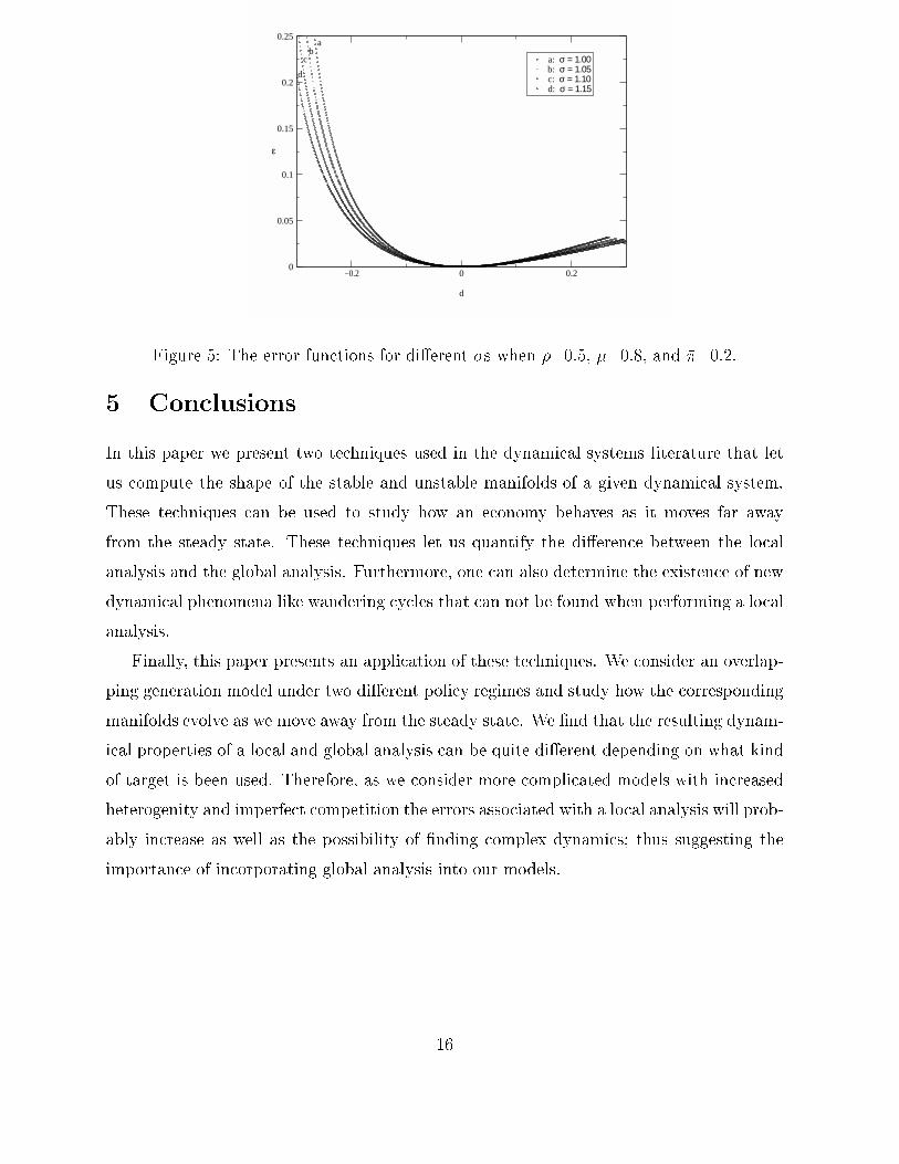
Finally, we explore how the linear error evolves as the money growth rate changes; see

Figure 5. We de�ne the error, �, as the distance between a point on the nonlinear manifold

and the corresponding point on the linear manifold, and d as the distance between the

steady state and a point on the linear manifold. The error decreases as the money growth

rate increases. As a result, the stable manifold becomes more linear since the dynamical

system is attracting points with greater \strength".

As we can see, the error associated with the local analysis is a decreasing function

of the money growth rate. Therefore, as we take into account the global properties of

the dynamical system the number of possible patterns corresponding to the predicted time

series increases. Finally, we note that the error function is not symmetric which emphasazies

the importance of how we approach the steady state. As a result, di�erent initial conditions

may result in di�erent speeds of convergence.

15

−0.2 0 0.2

d

0

0.05

0.1

0.15

0.2

0.25

ε

a: σ = 1.00b: σ = 1.05c: σ = 1.10d: σ = 1.15

ab

c

d

Figure 5: The error functions for di�erent �s when �=0.5, �=0.8, and ��=0.2.

5 Conclusions

In this paper we present two techniques used in the dynamical systems literature that let

us compute the shape of the stable and unstable manifolds of a given dynamical system.

These techniques can be used to study how an economy behaves as it moves far away

from the steady state. These techniques let us quantify the di�erence between the local

analysis and the global analysis. Furthermore, one can also determine the existence of new

dynamical phenomena like wandering cycles that can not be found when performing a local

analysis.

Finally, this paper presents an application of these techniques. We consider an overlap-

ping generation model under two di�erent policy regimes and study how the corresponding

manifolds evolve as we move away from the steady state. We �nd that the resulting dynam-

ical properties of a local and global analysis can be quite di�erent depending on what kind

of target is been used. Therefore, as we consider more complicated models with increased

heterogenity and imperfect competition the errors associated with a local analysis will prob-

ably increase as well as the possibility of �nding complex dynamics; thus suggesting the

importance of incorporating global analysis into our models.

16

References

[1] D.K. Arrowsmith and C.M. Place. An Introduction to Dynamical Systems. Cambridge

U. Press, 1990.

[2] C. Azariadis. Intertemporal Macroeconomics. Blackwell, 1995.

[3] G. Bischi, L. Gardini, and M. Kopel. Analysis of global bifurcations in a market share

attraction model. Journal of Economics Dynamics and Control, 24:855{879, 2000.

[4] X. Cabr�e, E. Fontich, and R. de la LLave. The parameterization method for invariant

manifolds: Manifolds associated to non-resonant subspaces. Manuscript, 1999.

[5] G. Debreu. Theory of Value: An Axiomatic Analysis of Economic Equilibrium. Wiley,

New York, 1959.

[6] D. Diamond and P. Dybvig. Bank runs, deposit insurance and liquidity. Journal of

Political Economy, 91:401{419, 1983.

[7] S. J. Fraser. The steady state and equilibrium approximations: A geometrical picture.

Journal of Chemical Physics, 88:4732{4738, 1998.

[8] J. Gaspar and K. Judd. Solving large-scale rational-expectation models. Macroeco-

nomic Dynamics, 1:45{75, 1997.

[9] S-M. Guu and K. Judd. Asymptotic methods for aggregate growth models. Journal

of Economic Dynamics and Control, 21:1025{42, 1997.

[10] K. Judd. Numerical Methods in Economics. Cambridge and London, MIT Press, 1998.

[11] A. Katok and B. Hasselblat. Introduction to Modern Theory of Dynamical Systems.

Cambridge U. Press, 1995.

[12] S. Schreft and B. Smith. The evolution of cash transactions: Some implications for

monetary policy. Journal of Monetary Economics, forthcoming, 2000.

[13] C. Sim�o. On the analytical and numerical approximation on invariant manifolds. Les

M�etodes Modernes de la M�ecanique C�eleste, Edited by D. Benest and C. Froeschl�e,

(Goutelas), 1989.

17

[14] S. Smale. Dynamics in general equilibrium theory. American Economic Review,

66:288{93, 1976.

[15] R. Townsend. Economic organization with limited communication. American Eco-

nomic Review, 77:954{971, 1987.

[16] M. Yokoo. Chaotic dynamics in a two dimensional overlapping generations model.

Journal of Economics Dynamics and Control, 24:909{934, 2000.

18