Quantifying the flux of CaCO3 and organic carbonfrom the surface ocean using in situ measurementsof O2, N2, pCO2, and pH

Steven Emerson,1 Christopher Sabine,2 Meghan F. Cronin,2 Richard Feely,2

Sarah E. Cullison Gray,3 and Mike DeGrandpre3

Received 22 July 2010; revised 11 March 2011; accepted 8 April 2011; published 16 July 2011.

[1] Ocean acidification from anthropogenic CO2 has focused our attention on theimportance of understanding the rates and mechanisms of CaCO3 formation so thatchanges can be monitored and feedbacks predicted. We present a method for determiningthe rate of CaCO3 production using in situ measureme nts of fCO2 and pH in surfacewaters of the eastern subarctic Pacific Ocean. These quantities were determined on asurface mooring every 3 h for a period of about 9 months in 2007 at Ocean Station Papa(50°N, 145°W). We use the data in a simple surface ocean, mass balance model ofdissolved inorganic carbon (DIC) and alkalinity (Alk) to constrain the CaCO3: organiccarbon (OC) production ratio to be approximately 0.5. A CaCO3 production rate of8 mmol CaCO3 m

−2 d−1 in the summer of 2007 (1.2 mol m−2 yr−1) is derived by combiningthe CaCO3: OC ratio with the a net organic carbon production rate (2.5 mol C m−2 yr−1)determined from in situ measurements of oxygen and nitrogen gas concentrationsmeasured on the same mooring (Emerson and Stump, 2010). Carbonate chemistry datafrom a meridional hydrographic section in this area in 2008 indicate that isopycnalsurfaces that outcrop in the winter in the subarctic Pacific and deepen southward into thesubtropics are a much stronger source for alkalinity than vertical mixing. This pathway hasa high enough Alk:DIC ratio to support the CaCO3:OC production rate implied by thefCO2 and pH data.

Citation: Emerson, S., C. Sabine, M. F. Cronin, R. Feely, S. E. Cullison Gray, and M. DeGrandpre (2011), Quantifying the fluxof CaCO3 and organic carbon from the surface ocean using in situ measurements of O2, N2, pCO2, and pH, Global Biogeochem.Cycles, 25, GB3008, doi:10.1029/2010GB003924.

1. Introduction

[2] The CaCO3: organic carbon (OC) mix of the particulateand dissolved material that exits the surface ocean stronglyinfluences the effect of the biological pump on the f CO2 ofthe atmosphere [e.g., Broecker and Peng, 1982; Sarmientoand Gruber, 2007; Emerson and Hedges, 2008]. This mix-ture also helps determine the depth at which the exportedparticulate organic matter degrades [Klaas and Archer, 2002;Armstrong et al., 2002], which greatly influences the effec-tiveness of themarine carbon pump on atmospheric f CO2 anddeep ocean oxygen concentration [Yamanaka and Tajika,1996; Kwon et al., 2009]. Thus, changes in the formationrate of CaCO3‐containing algae in response to anthropogenic

CO2 addition to the atmosphere will cause a carbon cyclefeedback that is presently difficult to predict.[3] Global estimates of the formation rate of CaCO3 in

ocean surface waters are based primarily on interpretation ofclimatological distributions of alkalinity (Alk) and dissolvedinorganic carbon (DIC) using seasonal changes in mixed‐layer alkalinity [Lee, 2001] and calculation of vertical fluxesbased on gradients in subsurface waters [Sarmiento et al.,2002; Moore et al., 2002; Jin et al., 2006]. In addition,Balch et al. [2007] have interpreted satellite measurement ofreflectance and color in terms of CaCO3 standing stocks.Global CaCO3 export rates derived from these methodsrange from 0.5 to 1.6 Gt C yr−1 (see Jin et al. [2006] andBerelson et al. [2007] for reviews). The fate of particulateCaCO3 after it leaves the upper ocean has been determinedby distinguishing the fraction of the measured water columnalkalinity that can be attributed to CaCO3 dissolution, TA*[Feely et al., 2002], by sediment trap experiments [e.g.,Honjo et al., 1995; Wong et al., 1999] and by sediment‐water dissolution and burial measurements [Hales andEmerson, 1997; Jahnke et al., 1994; Berelson et al., 2007].[4] This paper presents the results of the first successful

long‐term (9 month) autonomous in situ measurements of

1School of Oceanography, University of Washington, Seattle,Washington, USA.

2Pacific Marine Environmental Laboratory, NOAA, Seattle, Washington,USA.

3Department of Chemistry and Biochemistry, University of Montana,Missoula, Montana, USA.

Copyright 2011 by the American Geophysical Union.0886‐6236/11/2010GB003924

GLOBAL BIOGEOCHEMICAL CYCLES, VOL. 25, GB3008, doi:10.1029/2010GB003924, 2011

GB3008 1 of 12

both fCO2 and pH in open ocean surface waters, and itsinterpretation in terms of the ratio of CaCO3: OC produc-tion. We believe that this general method could be used toground truth the rates of CaCO3 production derived fromGCMs and satellites. The work presented here is the com-panion to another paper [Emerson and Stump, 2010] inwhich in situ measurements of O2 and N2 from the samemooring deployment were interpreted in terms of net com-munity production (NCP) of oxygen and organic matter. Bycombining these results with simultaneous measurementsof fCO2 and pH we constrain the CaCO3: OC formationratio to be about 0.5 and the CaCO3 production rate to be∼8 mmol m−2 d−1 in the summer of 2007 in the subarcticPacific Ocean. We show that the likely transport pathwayfor resupplying alkalinity removed from North Pacific sur-face waters is along isopycnal surfaces that plunge intodeeper waters to the south rather than by vertical processesassumed in the earlier studies.

2. Setting and Methods

2.1. Station Papa

[5] The subarctic Pacific Ocean at Ocean Station Papa(hereafter Stn. P, located at 50°N, 145°W) is a region whereprecipitation and fresh water runoff from the continentsexceeds evaporation leading to a layer of low‐salinity waterthat caps a permanent halocline. There is a strong season-ality in temperature in surface waters (Figure 1a). In winterthe Aleutian low is positioned in the Gulf of Alaska andbrings winds that average 12 m s−1 which combine withcold temperatures (<6°C) to mix the surface layer to depthsof the halocline at about 110 m. In summer the Aleutian lowmoves northward and wind speeds drop to an average of7–8 m s−1 allowing the formation of a shallower thermocline

and the mixed layer decreases to 25–30 m as the waterswarm. Geostrophically driven surface currents in the sub-arctic region north of 42°N are characterized by cycloniccirculation in which the flow west of 140°W and south of55°N is to the east [Favorite et al., 1976], with a surfaceEkman flow in the vicinity of Stn P to the southeast. In aclassic interpretation of the hydrographic data from weatherships during the period of the 1950s and 1960s, Tabata[1961] showed that the salt balance in the region con-strains upward advection across the halocline to an annuallyaveraged value of 10–20 m yr−1. This work and more recentstudies [Large et al., 1986; Archer et al., 1993; Large et al.,1994] demonstrated that a one dimensional heat and nutrientbudget is pretty well closed in summer, but in the fall andwinter horizontal fluxes become an important component ofthe transport.[6] The macronutrients dissolved inorganic nitrogen (DIN)

and dissolved inorganic phosphate (DIP) are above detectionlimits by traditional methods in surface waters of the high‐latitude North Pacific Ocean year‐round. Wong et al. [2002]demonstrated using 2 years of surface water sampling fromcontainer ships that NO3

− levels drop from values of about17 mmol kg−1 in winter to about 8 mmol kg−1 in Augustand September. These changes were interpreted alongwith Redfield stoichiometry (DC: DN = 6.6) to indicatea summertime carbon export from the mixed layer of∼19 mmol C m−2 d−1. This result is very similar to that deter-mined based on oxygen mass balance (17 mmol C m−2 d−1)using in situ O2 and N2 measurements [Emerson and Stump,2010]. The latter result was determined from a simple upperocean model and in situ measurements of the degree ofsupersaturation of oxygen and nitrogen (see Figure 1b). Netbiological oxygen production determined from these data isproportional to the difference in supersaturation betweenoxygen and nitrogen gas (DO2 − DN2), which is very largeduring summer and effectively non existent in winter. Weused these data to suggest that almost all of the net biologicalcarbon production in this area was in summer [Emerson andStump, 2010], and our interpretation of the fCO2 and pH datain this paper will also focus in the period of June‐October2007.[7] A convenient aspect of studying the carbonate chem-

istry in the northeast subarctic Pacific is that Sta P has beenthe site of intensive studies of particle fluxes [Wong et al.,1999; D. Timothy et al., The climatology and nature ofsettling particles in the subarctic northeast Pacific Ocean basedon 24 years of sediment‐trap flux, submitted to Progress inOceanography, 2011], dissolved inorganic carbon changes[Wong et al., 2002] and biological calcification [Lipsen et al.,2007]. In the DISCUSSION section we evaluate the efficacyof our in situ measurements and model by comparing ourresults of net organic carbon and CaCO3 production withthose from previous observations.

2.2. Mooring Time Series Methods

[8] We report approximately 1 year of data from a heavilyinstrumented surface mooring deployed at Stn. P that startedin June 2007 and now continues as a NOAA contribution tothe global network of OceanSITES reference stations. Thesurface meteorological suite of sensors on the mooringincluded a Gill sonic anemometer that made a 2 min averageof wind speed and direction measurements every 10 min.

Figure 1. Changes in (a) temperature and (b) the degree ofsupersaturation of oxygen and nitrogen in the surface watersat Stn P (50°N and 145°W). Notice the evolution of the dif-ference between O2 and N2 supersaturation between summerand winter. These data were used in a simple upper oceanmodel to determine the net biological O2 production in acompanion paper [Emerson and Stump, 2010].

EMERSON ET AL.: IN SITU pCO2 AND pH GB3008GB3008

2 of 12

Surface ocean temperature and salinity were measured at10 min intervals at 1 m, 5 m, 8 m, 10 m, 35 m, 45 m, (and5 more depths down to 200 m), and at hourly intervals at20 m. An hourly time series of the mixed‐layer depth wascomputed by determining the depth at which the density was0.2 kg m−3 larger than the 1 m surface value. Currents weremeasured every 20 min at 5 m and 35 m depths using Sontekacoustic Doppler current meters. Data from this project canbe found on the Web at http://www.pmel.noaa.gov/stnP/.[9] Measurements of oxygen and total gas tension at two

meters depth were used to determine the concentrations ofO2 and N2. These methods and data have been presented andinterpreted previously [Emerson and Stump, 2010]. Here wefocus on describing the utility of fCO2 and pH measure-ments in determining the contribution of CaCO3 formationto the local carbon cycle. (See Cullison Gray et al. [2011] fora more general evaluation of calculating inorganic carbonspecies from pH and fCO2 measurements.)[10] The mole fraction of carbon dioxide was measured

at a depth of about one meter and in the atmosphere every3 h using the NOAA/PMEL‐built MAPCO2 system. Thissystem uses an automated bubble equilibrator‐based gascollection system with an infrared gas analyzer (Li‐820,Li‐Cor Biogeosciences, Incorporated, Lincoln, Nebraska).The equilibrator is based on the design of Friederich et al.[1995]. Calibration is performed immediately prior to theatmospheric and surface ocean measurements using a CO2

calibration span gas that has been compared to standards fromNOAA/ESRL which are traceable to World MetrologicalOrganization (WMO) references. System accuracy is esti-mated to be 1–2 ppm based on laboratory calibrations, fieldcomparisons with underway CO2 systems, and internationalintercomparison exercises. Data and diagnostic informationare transmitted from the system to PMEL daily and posted onthe Web in near‐real time (http://www.pmel.noaa.gov/co2/moorings/papa/papa_main.htm).[11] pH measurements were made every 3 h with a

Sunburst Sensors automated pH sensor that was attached to

the mooring bridle at a depth of about 2 m. Hydrogen ionconcentrations are determined with this instrument spectro-photometrically using a sulphonephthalein indicator thatdevelops a pH‐dependent color [Martz et al., 2003; Seidelet al., 2008]. Because small samples are used and a rathershort path length is necessary, the effect of the reagentaddition on the in situ pH is determined by using a dyedilution curve and extrapolating the measured absorptionreadings to the values for zero added reagent. The methodis precise to better than ±0.001 pH unit and accurate to±0.002 pH units based on laboratory tests in which results ofthe in situ instrument were compared with those determinedby hand on a laboratory spectrophotometer. Data from theinstrument was recorded internally and downloaded when itwas retrieved during buoy replacement (once each year).

2.3. Seawater Hydrography and Carbonate Chemistry

[12] We also present carbonate chemistry and hydro-graphic data from a University of Washington StudentCruise on the R. V. Thompson between Ocean Station P andHawaii in August/September 2008 (TN224). The cruisetrack headed south from Stn P (145°W, 50°N) to 38°N, thenjogged north to 45°N and 152°W where it again turnedsouth and followed the meridional transect occupied previ-ously by CLIVAR P16 along 152°W. (See Howard et al.[2010] for more information about the cruise.) Hydrographicstations were occupied every 2 degrees with sampling todepths of 1000–2000 m. Dissolved inorganic carbon (DIC)was analyzed by coulometry [Johnson et al., 1998] and alka-linity by open‐cell potentiometric titration [Millero et al.,1998; Dickson et al., 2003]. Certified reference materials[Dickson et al., 2003] were used to validate accuracy of bothmethods. Duplicate analysis of reference materials and sam-ples indicate a precision of ±2 mmol kg−1 and ±4 meq kg−1 forDIC and Alk, respectively.

3. Results

3.1. Surface Ocean fCO2 and pH Time Series

[13] Data from June 2007 to February 2008 (Figure 2)indicate seasonal changes of ∼55 ppm for fCO2 and ∼0.04 pHunits. Scatter around the daily averaged trends presented inFigure 2 is on the order of the errors reported above. ThefCO2 values are near atmospheric equilibrium (375–390)with slight supersaturation in summer and undersaturation inwinter, which is similar to earlier seasonal fCO2 data fromthis time series location [Wong and Chan, 1991]. The pHmeasurements follow a trend opposite to that of fCO2. Dataassociated with each measurement indicated that the line-arity in the trend of pH absorbance versus volume of addedreagent during the dye dilution curves began to deteriorate(dropped below r2 = 0.99) after November 2007 (∼day 330).We do not interpret the pH data after this time because ofuncertain accuracy. There is not a third measurement of thecarbonate system from the same location and time for anindependent check on the accuracy of these measurements.We will show, however, that the formation rate of CaCO3

depends mainly on the observed changes in pH and fCO2

rather than absolute values. Thus, small inaccuracies thatcould exist will not affect our conclusions. Drift in the pHdata due to biofouling, however, could be a problem, and in

Figure 2. Surface water fCO2 (dark asterisk), pH (redcross), and atmospheric fCO2 (dark square) at Stn P fromJune 2007 till about February 2008. Daily averages are plot-ted from measurements every 3 h by in situ sensors on a sur-face mooring.

EMERSON ET AL.: IN SITU pCO2 AND pH GB3008GB3008

3 of 12

current field studies we are determining Alk and DIC at eachopportunity to empirically determine stability.

3.2. Hydrographic Data From TN224

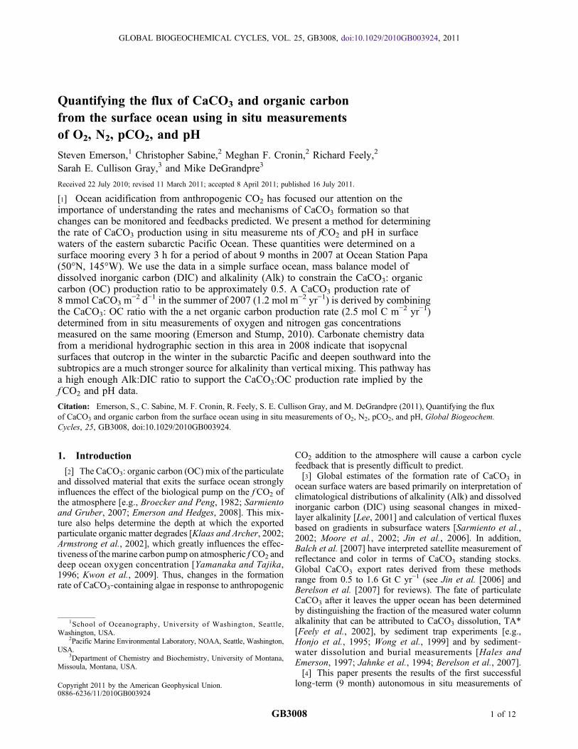
[14] A section of the hydrographic data from the StudentCruise in 2008 is presented in Figure 3. Meridional trendsalong 152°W are shown as a function of depth and density.The low‐salinity waters of the surface subarctic Pacificcontrast the high‐salinity waters in the subtropics (Figure 3a).Meridional trends in surface water alkalinity follow thoseof salinity much more closely than do DIC changes(Figures 3b and 3c) indicating the more conservativebehavior of alkalinity [Lee et al., 2006]. The carbonate ionconcentration (Figure 3d) was calculated from DIC andAlkalinity using the apparent constants for the carbonateequilibria presented by Lueker et al. [2000]. The dashed linein Figure 3d indicates the saturation horizon for aragonite(aragonite is supersaturated above and undersaturatedbelow) using the aragonite solubility product presented byMucci [1983] and assuming calcium is a conservative ion in

seawater and varies only with salinity. The saturation hori-zon follows s� ∼ 26.5 which plunges from depths just belowthe euphotic zone at 50°N to between 400 and 500 m in thesubtropics.

4. Discussion

4.1. Carbonate Equilibrium

[15] Changes in the pH and fCO2 of surface seawaterdepend on temperature, salinity and reactions that alterdissolved inorganic carbon and total alkalinity. We dem-onstrate these effects on the data by calculating the car-bonate ion concentration (Figure 4 and equation (1)) frommeasured pH and fCO2. Chemical equilibrium constantsused in the calculation are: the Henry’s Law coefficient forCO2 solubility in seawater (KH,Weiss [1974]), and the valuesreported by Lueker et al. [2000] for the hydration of CO2 toHCO3 (K1′ ) and the equilibrium between HCO3

− and CO32−

(K2′ ). Lueker et al. [2000] demonstrated that the dissociationconstants determined by Mehrbach et al. [1973] interpretedon the “total hydrogen scale” give internally consistent resultswhen combined with highly precise measurements of Alk,DIC and fCO2 values below 500 micro atmospheres.

CO2�3

� � ¼ KHK1′K2′f CO2

Hþ½ �2 ð1Þ

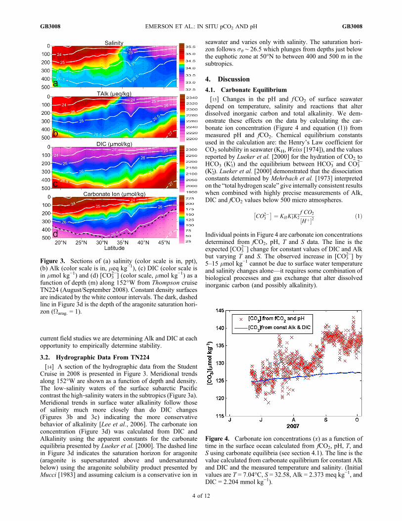
Individual points in Figure 4 are carbonate ion concentrationsdetermined from fCO2, pH, T and S data. The line is theexpected [CO3

2−] change for constant values of DIC and Alkbut varying T and S. The observed increase in [CO3

2−] by5–15 mmol kg−1 cannot be due to surface water temperatureand salinity changes alone—it requires some combination ofbiological processes and gas exchange that alter dissolvedinorganic carbon (and possibly alkalinity).

Figure 3. Sections of (a) salinity (color scale is in, ppt),(b) Alk (color scale is in, meq kg−1), (c) DIC (color scale isin mmol kg−1) and (d) [CO3

2−] (color scale, mmol kg−1) as afunction of depth (m) along 152°W from Thompson cruiseTN224 (August/September 2008). Constant density surfacesare indicated by the white contour intervals. The dark, dashedline in Figure 3d is the depth of the aragonite saturation hori-zon (Warag. = 1).

Figure 4. Carbonate ion concentrations (x) as a function oftime in the surface ocean calculated from fCO2, pH, T, andS using carbonate equilibria (see section 4.1). The line is thevalue calculated from carbonate equilibrium for constant Alkand DIC and the measured temperature and salinity. (Initialvalues are T = 7.04°C, S = 32.58, Alk = 2.373 meq kg−1, andDIC = 2.204 mmol kg−1).

EMERSON ET AL.: IN SITU pCO2 AND pH GB3008GB3008

4 of 12

[16] To a first‐order approximation the change in carbonateion concentration due to biological processes depends on thedifference in the changes of Alk and DIC:

Alk � DIC ffi HCO�3

� �þ 2 CO2�3

� �þ HBO�4

� �� �� HCO�3

� �þ CO2�3

� �� �DAlk �DDIC ffi D CO2�

3

� � ð2Þ

[17] The second relationship above is approximate pri-marily because it assumes the borate ion component of thealkalinity is constant, whereas it is a function of pH.Emerson and Hedges [2008, Table 4.8] demonstrate thatduring addition of CO2 to surface waters about 60% of thecarbonate ion change, D[CO3

2−], expected from the aboveapproximation is realized. Degassing of CO2 because of theslight fCO2 supersaturation in August and September(Figure 2) would cause a decrease in DIC and thus anincrease in [CO3

−2]. We show later, however, that gasexchange is only a small flux compared to organic carbonexport determined from the oxygen mass balance in summersuggesting that gas exchange plays a minor role in thesurface ocean carbon balance. If organic matter formationwere the only process affecting the dissolved inorganiccarbon in ocean surface waters during photosynthesis, DICwould decrease while Alk increased, increasing [CO3

−2].(During organic matter formation,DAlk ∼ −(16/106) ×DDIC,assuming Redfield Ratio changes for N and organic C.)Surface water summertime decrease in DIC in the subarcticPacific has been observed previously to be about −80mmol kg−1

[Wong et al., 2002]. If this change were due only to organiccarbon production, with the resulting increase of 12 meq kg−1

in alkalinity, it would result in an increase of the carbonate ionconcentration of 58 mmol kg−1, which is much greater thanthe observations in Figure 4.

[18] During CaCO3 formation Alk decreases at twice therate of DIC indicating that CaCO3 precipitation alone wouldcause [CO3

2−] to decrease with time in surface waters.Qualitatively, fCO2 and pH changes that result in the small,∼10 mmol kg−1, [CO3

2−] increase during summer requireformation of calcium carbonate and organic matter. In thefollowing discussion we use a simple mass balance model toconstrain the rates of CaCO3 and organic matter formation.

4.2. The Rates of Organic Carbon and CaCO3

Production

[19] Emerson and Stump [2010] determined net commu-nity organic carbon production during the summer of 2007at Stn P using oxygen and nitrogen data along with a mixed‐layer model. The model assumed a well‐mixed surface layerof water that is open to gas exchange at the air‐water interfaceand water exchange along and across isopycnals via advec-tion and mixing (Figure 5). Since a detailed description ofthe model was presented previously, we review it onlybriefly here. The time rate of change of solute concentration,[C] (mol m−3), in a mixed layer of depth h (m) is equal tothe sum of air‐water exchange, mixing and biologicalproduction.

hd C½ �.dt ¼ FA�W þ E þ Av þ Az þMz þM� þ JC ð3Þ

Terms on the right hand side are: air‐water gas exchange,FA‐W (mol m−2 d−1); entrainment due to mixed layer deep-ening, E; horizontal advection in the mixed layer, Av; ver-tical exchange, either by upwelling, Az, or mixing along andacross density surfaces, Mz and Ms, respectively; andfinally biological production, JC. Each term for the physicalprocesses is the product of a mass transfer coefficient or

Figure 5. A schematic representation of the model used to determine net biological fluxes from themixed layer at Stn P. Dashed lines represent constant density surfaces, and h is the mixed layer depth.J is the net biological production and export (equation (3)). Other symbols associated with arrows aremass transfer coefficients that appear in equations (4)–(8). They are the mass transfer coefficients for gasexchange, k (equation (4)), and bubble air injection, Vinj (equation (4)); advection velocities in both thehorizontal, v (equation (5)), and vertical, w (equation (6)), directions; and eddy diffusion coefficientsacross, Kz (equation (7)), and along, Ks (equation (8)), isopycnal surfaces.

EMERSON ET AL.: IN SITU pCO2 AND pH GB3008GB3008

5 of 12

mixing term and measured concentration or concentrationgradients. The mass transfer coefficients and mixing termsare identified in Figure 5 and in the following equations.These quantities must be either measured or estimated fromprevious studies of physical processes in this region todetermine the net biological carbon production, JC.[20] We solve equation (3) for DIC and Alk using O2 and

N2‐determined organic carbon production rates and a rangeof CaCO3: OC production ratios. The terms of equation (3)that were most influential in controlling the summertimemass balance of O2 and N2 [Emerson and Stump, 2010]were the time rate of change and air‐water gas transfer.Transport across the base of the mixed layer in summer byvertical advection and diffusion had minor influence. Localchanges and air‐water gas exchange are most important inthe O2 and N2 mass balance because residence times ofthese gases with respect to air‐sea exchange are relativelyshort: on the order of a few weeks to a month. This is not thecase for dissolved inorganic carbon because the [CO2] gas isonly a small component of the DIC in the mixed layer,and its residence time with respect to gas exchange is about10 times that for oxygen and nitrogen. Local concentrationchanges of dissolved inorganic carbon and alkalinity aremore influenced by mixing and advection than are O2 andN2, thus processes occurring in the greater subarctic northPacific have more influence in the DIC and Alk mass bal-ances. In the following paragraphs we briefly describe howeach of the terms on the right side of equation (3) and thecoefficients in Figure 5 were evaluated.[21] The air water exchange term is normally separated

into a diffusive flux, G (mol m−2 d−1) and a bubble flux, B.The first is characterized by the mass transfer coefficient forgas exchange, kC (m d−1), multiplied by the difference in

concentration of the gas in the mixed layer and that at sat-uration equilibrium with the atmosphere, [Csat].

F ¼ Gþ B ¼ kC CO2½ � � CO2sat½ �� �þ Vinj XC ð4Þ

The air injection mechanism of bubble processes is param-eterized by a mass transfer coefficient, Vinj, and the molefraction of gas C in the atmosphere, XC [e.g., Hamme andEmerson, 2006]. While bubble processes have a largeinfluence on the gas exchange of insoluble gases like O2 andN2, they are not very important for the more soluble CO2,and they are ignored here. The concentrations of dissolvedCO2 in the mixed layer and the value in equilibrium withthe atmosphere ([CO2] and [CO2

sat]) are calculated from theocean and atmosphere fCO2 data in Figure 2 using the sol-ubility of CO2 in seawater. The mass transfer coefficient, kC,is dependent on the physical properties of the gas and solutevia the Schmidt number, SC = (n/D), where n (cm2 s−1) isthe kinematic viscosity of the liquid and D (cm2 s−1) themolecular diffusion coefficient of the gas (see Emerson andHedges [2008, chap. 9] for more details). The mass transfercoefficient has been correlated with wind speed in surfaceocean purposeful tracer release experiments. We determinethe mass transfer coefficient normalized to kCO2 at 20°C andS = 35 using the relationship to wind speed presented byNightingale et al. [2000].[22] Entrainment is active only when the mixed layer

deepens in the fall and winter. Since we interpret the dataonly through September, this term is of little importance tillthe very latter part of the period of interest when con-centrations below the mixed layer are incorporated while themixed layer deepens.[23] Ekman transport is assumed to dominate the advec-

tive flow in the mixed layer, h, which is about 30 m deepduring most of the summer.

Av ¼ u d C½ ��dx

hþ v d C½ �

�dy

h ð5Þ

Here, u and v (m d−1) are the zonal and meridional com-ponents of surface currents. Ekman transport at Stn P isgreater in winter than summer because of the variability inwind speed [Roden, 1977; Ayers and Lozier, 2010]. Windsare mainly to the east resulting in a southward vector ofvelocity that reaches values of ∼0.1 m s−1 in the wintertime.(See results from the global ocean data assimilation System,http://ferret.pmel.noaa.gov/NVODS). We consider the south-ward component of the surface transport to be the mostimportant because both meridional currents and concentrationgradients are strongest. Both atmospheric wind and surfaceocean current velocities were measured on the mooring in2007 (data not presented). The southward component of thesurface currents during the period of June to October 2007was variable and small averaging essentially zero from 5 mdepth measurements and 0.01 m s−1 from Ekman transportcalculations. We use advection velocities that incorporate thisrange of measurements in the sensitivity analysis describedbelow.[24] Mixed layer concentration gradients of salinity‐

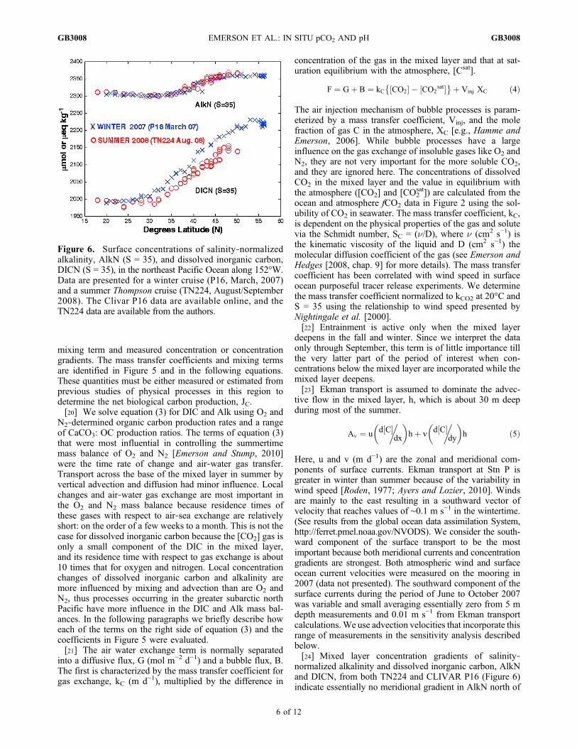
normalized alkalinity and dissolved inorganic carbon, AlkNand DICN, from both TN224 and CLIVAR P16 (Figure 6)indicate essentially no meridional gradient in AlkN north of

Figure 6. Surface concentrations of salinity‐normalizedalkalinity, AlkN (S = 35), and dissolved inorganic carbon,DICN (S = 35), in the northeast Pacific Ocean along 152°W.Data are presented for a winter cruise (P16, March, 2007)and a summer Thompson cruise (TN224, August/September2008). The Clivar P16 data are available online, and theTN224 data are available from the authors.

EMERSON ET AL.: IN SITU pCO2 AND pH GB3008GB3008

6 of 12

the subarctic‐subtropical boundary, but a strong gradient inDIC which decreases to the south. Because curvature in thehorizontal gradient is difficult to quantify from this data, weassume two extreme cases for horizontal advection of DIC.The minimum influence of meridional advection is repre-sented by no divergence of flux at 50°N: the advective fluxfrom the north equals that to the south. In the other extremewe assume no horizontal gradient north of 50°N so thatmeridional advection along the gradient south of Stn P wouldlower DICN without influencing AlkN causing a positiveDAlk − DDIC, and hence an increase in [CO3

2−].[25] Vertical advection across the base of the summer

mixed layer is described by:

Az ¼ w d C½ ��dz

Dz ð6Þ

where w (m d−1) is the upwelling velocity, and Dz repre-sents the depth scale for vertical transport which we take tobe the mixed layer depth. The high end of the range ofvertical advection velocities calculated previously for thisregion is on the order of 1 × 10−6 m s−1 (Tabata [1961] andSasai and Ikeda [2003], w ∼ 0.1 m d−1). These values aredominated by winter time upwelling and the value wedetermine from satellite wind stress curl patterns during thesummer of 2007 is 100 times smaller and negligible in thetransport balance.[26] Vertical mixing across the base of the mixed layer is

depicted as:

Mz ¼ Kzd C½ �

�dz

ð7Þ

where Kz (m2 s−1) is the vertical eddy diffusion coefficient

(see Figure 5). Diapycnal mixing processes are difficult toevaluate, but are potentially important because of the stronggradient in DIC between the surface mixed layer andthe region below. (From the data in Figure 3, the DIC dif-ference between 25 and 75 m depth in August of 2008 was∼50 mmol kg−1, whereas the gradient in Alk was negligible.)A minimum value for the vertical eddy diffusion coefficientis that estimated within the thermocline by microstructuremeasurements [Gregg, 1989] and measured by tracer releaseexperiments [e.g., Ledwell et al., 1998], 0.1–0.2 × 10−4 m2 s−1.However, Large et al. [1986] showed that during storms,diffusive mixing across the base of the mixed layer at Stn Pcan be characterized by eddy diffusion coefficients up to onehundred times this value over short periods of time. Weassume Kz = 0.1 × 10−4 m2 s−1 is a lower limit and solve forvalues that are three times and ten times greater to determinethe sensitivity to diapycnal mixing.[27] Transport along density surfaces in the subarctic

Pacific is also a vertical exchange because the depth of thedensity horizons representing the base of the winter mixedlayer at Stn P (50°N) (s� ∼ 26.2) plunges to ∼200 m at 40°Nand ∼400 m at 30°N. Mixing along isopycnal surfaces isdescribed by the diffusion equation:

M� ¼ K�d C½ �

�dl

ð8Þ

where l is the distance along the isopycnal surface and Ks(m2 s−1) is the isopycnal eddy diffusion coefficient. This

process connects the mixed layer in winter and water belowthe mixed layer in summer with deeper thermocline watersto the south. Isopycnal mixing does not play a role in thesummertime mass balance of the mixed layer because it isisolated by thermal stratification. However, as we shall see,it is an important process balancing biological removal ofCaCO3 on an annual basis.[28] We calculate the change in Alk and DIC in the mixed

layer at Stn P using the same mass transfer coefficientsemployed to constrain the O2 and N2 mass balance[Emerson and Stump, 2010]. The value of the net biologicaloxygen production was transformed to net organic carbonproduction and DIC decrease using a DC/DO2 ratio of−1/1.45 [Hedges et al., 2002]. Initial alkalinity and DIC inthe mixed layer are given values near those measured at152°N (Figure 3) but adjusted to exactly match the fCO2

and pH measured at Stn P in June 2007. Equation (3) isstepped forward in time and the f CO2 and pH are recalculatedby the chemical equilibrium equations after each time step.The process is completed for ratios of calcium carbonate toorganic carbon export rates of, CaCO3: OC = 0.0, 0.5 and 1.0,and for the range of advection and diapycnal eddy diffusiondiscussed above. Net biological organic carbon productionrates determined from O2 and N2 mass balance are relativelyinsensitive (±20%) to this range of mixing parameters.[29] Results of the calculations are presented in Figure 7

and Table 1. The top three panels of Figure 7 are solutionsfor a diapycnal eddy diffusion coefficient of 0.1 × 10−4 m2 s−1.The bottom three solutions are the changes derived for aneddy diffusion coefficient three times this value. In order tomatch the observed fCO2 and pH with low Kz (Figure 7,Case I), it is necessary to have a CaCO3: OC ratio of at least0.5. No production of CaCO3 results in fCO2 and pH trendsless than those observed and a value of CaCO3: OC = 1.0creates trends in the correct sense but too extreme.Increasing the vertical eddy diffusion coefficient (Figure 7,Case II) makes it possible to match the f CO2 and pH datausing a CaCO3: OC = 0.0, but we show in the followingparagraph describing the results in Table 1 that this caseviolates other constraints.[30] The sensitivity analysis in Table 1 compares results

from different model runs with observed changes in sum-mertime f CO2 and pH (as in Figure 7) and also withexpected changes in Alk and DIC. Expected alkalinitychanges are determined from carbonate equilibrium withf CO2 and pH. Because calculated alkalinity is susceptible tosmall errors in these measurements, we assume a wide rangeof acceptable alkalinity change in the row labeled “MeasuredValues” of Table 1. The constraint for summertime change inDIC is taken from previous measurements during the sum-mertime in the eastern subarctic Pacific of ∼−80 mmol kg−1

over a period of 2 years (1995–1997 [Wong et al., 2002])from container ship crossings from Asia to Western NorthAmerica. Because these data are from an earlier time, weassume an acceptable value for 2007 to be somewhere in therange of DDIC = −(50–100) mmol kg−1.[31] The sensitivity analysis was carried out for a south-

ward component of advection in the surface layer of 0 and0.01 m s−1; however, only the results for v = 0.01 m s−1 arepresented in Figure 7 and Table 1 because horizontaladvection of this magnitude made little difference in thepredicted changes. Bold values of the “Model Results” in

EMERSON ET AL.: IN SITU pCO2 AND pH GB3008GB3008

7 of 12

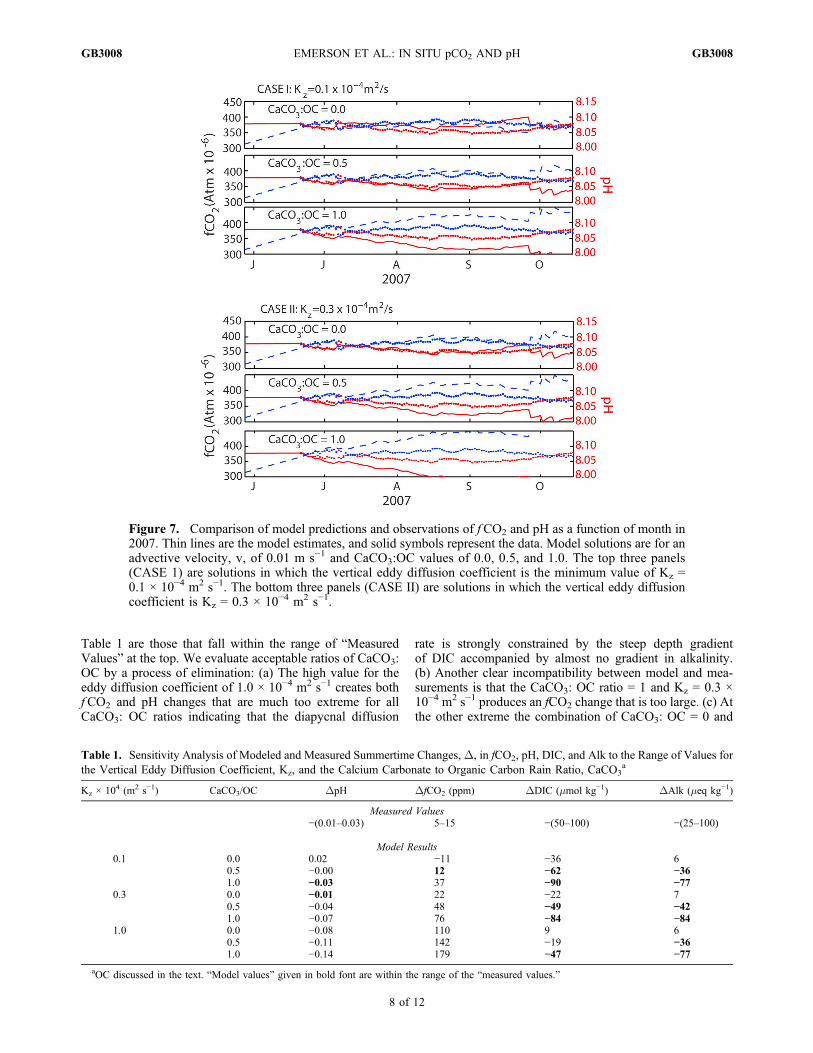
Table 1 are those that fall within the range of “MeasuredValues” at the top. We evaluate acceptable ratios of CaCO3:OC by a process of elimination: (a) The high value for theeddy diffusion coefficient of 1.0 × 10−4 m2 s−1 creates bothfCO2 and pH changes that are much too extreme for allCaCO3: OC ratios indicating that the diapycnal diffusion

rate is strongly constrained by the steep depth gradientof DIC accompanied by almost no gradient in alkalinity.(b) Another clear incompatibility between model and mea-surements is that the CaCO3: OC ratio = 1 and Kz = 0.3 ×10−4 m2 s−1 produces an fCO2 change that is too large. (c) Atthe other extreme the combination of CaCO3: OC = 0 and

Figure 7. Comparison of model predictions and observations of f CO2 and pH as a function of month in2007. Thin lines are the model estimates, and solid symbols represent the data. Model solutions are for anadvective velocity, v, of 0.01 m s−1 and CaCO3:OC values of 0.0, 0.5, and 1.0. The top three panels(CASE 1) are solutions in which the vertical eddy diffusion coefficient is the minimum value of Kz =0.1 × 10−4 m2 s−1. The bottom three panels (CASE II) are solutions in which the vertical eddy diffusioncoefficient is Kz = 0.3 × 10−4 m2 s−1.

Table 1. Sensitivity Analysis of Modeled and Measured Summertime Changes,D, in fCO2, pH, DIC, and Alk to the Range of Values forthe Vertical Eddy Diffusion Coefficient, Kz, and the Calcium Carbonate to Organic Carbon Rain Ratio, CaCO3

a

Kz × 104 (m2 s−1) CaCO3/OC DpH DfCO2 (ppm) DDIC (mmol kg−1) DAlk (meq kg−1)

Measured Values−(0.01–0.03) 5–15 −(50–100) −(25–100)

Model Results0.1 0.0 0.02 −11 −36 6

0.5 −0.00 12 −62 −361.0 −0.03 37 −90 −77

0.3 0.0 −0.01 22 −22 70.5 −0.04 48 −49 −421.0 −0.07 76 −84 −84

1.0 0.0 −0.08 110 9 60.5 −0.11 142 −19 −361.0 −0.14 179 −47 −77

aOC discussed in the text. “Model values” given in bold font are within the range of the “measured values.”

EMERSON ET AL.: IN SITU pCO2 AND pH GB3008GB3008

8 of 12

Kz = 0.1 × 10−4 creates fCO2 and pH changes in the oppositesense to those measured.[32] We have now eliminated all but the 2–5th rows in

Table 1. All these scenarios are within or close to theacceptable range of fCO2 and pH change. Only the case forCaCO3: OC = 0 and Kz = 0.3 × 10−4 m2 s−1 clearly violatesacceptable trends in DIC and Alk. The predicted alkalinitychange for this scenario is positive, which is in dramaticcontrast to the change required for chemical equilibriumwith f CO2 and pH (−25 to −100 meq kg−1). Also, thecalculated DDIC of −23 mmol kg−1 is much smaller forthis case than previously measured summertime changes of−(50–100) mmol kg−1.[33] In order to meet the constraints of the temporal

changes of the carbonate system as determined by timeseries measurements of fCO2, pH and previous measure-ments of DIC change in summer our model suggests that theCaCO3: OC ratio must be on the order of 0.5. Acceptablevalues are between 0.5 and 1.0 for Kz = 0.1 × 10−4 m2 s−1

and <0.5 for Kz = 0.3 × 10−4 m2 s−1. Combining the CaCO3:OC ratio with the organic carbon production rate of17 mmol m−2 d−1 results in a flux of CaCO3 from the surfaceocean in this region of ∼8 mmol m−2 d−1.

4.3. Alkalinity Mass Balance for the Upper Oceanin the Subtropical Pacific

[34] If the CaCO3 is being produced at a rate that is abouthalf of that of organic carbon in the subarctic Pacific insummer, what are the processes that supply alkalinity to thesurface waters? Horizontal fluxes via surface water transportare negligible in this area of the subarctic Pacific because ofsmall gradients both meridionally (Figure 6) and zonally(data not shown). Vertical transport of DIC and Alkalinityhave been used to estimate the CaCO3: Organic C produc-tion rate ratio of 0.05–0.1 for the world’s ocean with theNortheast Pacific near Stn P in this range [Sarmiento et al.,2002; Jin et al., 2006]. These values are much smaller than

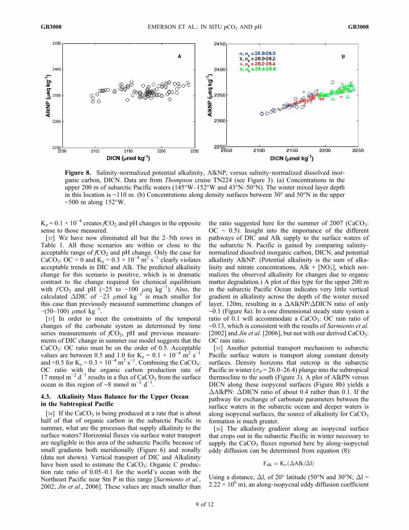
the ratio suggested here for the summer of 2007 (CaCO3:OC ∼ 0.5). Insight into the importance of the differentpathways of DIC and Alk supply to the surface waters ofthe subarctic N. Pacific is gained by comparing salinity‐normalized dissolved inorganic carbon, DICN, and potentialalkalinity AlkNP. (Potential alkalinity is the sum of alka-linity and nitrate concentrations, Alk + [NO3

−], which nor-malizes the observed alkalinity for changes due to organicmatter degradation.) A plot of this type for the upper 200 min the subarctic Pacific Ocean indicates very little verticalgradient in alkalinity across the depth of the winter mixedlayer, 120m, resulting in a DAlkNP/DDICN ratio of only∼0.1 (Figure 8a). In a one dimensional steady state system aratio of 0.1 will accommodate a CaCO3: OC rain ratio of∼0.13, which is consistent with the results of Sarmiento et al.[2002] and Jin et al. [2006], but not with our derived CaCO3:OC rain ratio.[35] Another potential transport mechanism to subarctic

Pacific surface waters is transport along constant densitysurfaces. Density horizons that outcrop in the subarcticPacific in winter (s� = 26.0–26.4) plunge into the subtropicalthermocline to the south (Figure 3). A plot of AlkPN versusDICN along these isopycnal surfaces (Figure 8b) yields aDAlkPN: DDICN ratio of about 0.4 rather than 0.1. If thepathway for exchange of carbonate parameters between thesurface waters in the subarctic ocean and deeper waters isalong isopycnal surfaces, the source of alkalinity for CaCO3

formation is much greater.[36] The alkalinity gradient along an isopycnal surface

that crops out in the subarctic Pacific in winter necessary tosupply the CaCO3 fluxes reported here by along‐isopycnaleddy diffusion can be determined from equation (8):

Falk ¼ K� DAlk=Dlð Þ

Using a distance, Dl, of 20° latitude (50°N and 30°N; Dl =2.22 × 106 m), an along‐isopycnal eddy diffusion coefficient

Figure 8. Salinity‐normalized potential alkalinity, AlkNP, versus salinity‐normalized dissolved inor-ganic carbon, DICN. Data are from Thompson cruise TN224 (see Figure 3). (a) Concentrations in theupper 200 m of subarctic Pacific waters (145°W–152°W and 43°N–50°N). The winter mixed layer depthin this location is ∼110 m. (b) Concentrations along density surfaces between 30° and 50°N in the upper∼500 m along 152°W.

EMERSON ET AL.: IN SITU pCO2 AND pH GB3008GB3008

9 of 12

Ks = 1000 m2 s−1 [Ledwell et al., 1998; Gananadesikanet al., 2002] and an alkalinity flux necessary to maintain aCaCO3 flux of 8 mmol m−2 d−1 (Falk = 16 meq m2 d−1)results in an alkalinity increase of only about one micro-equivalent over a distance of 20 degrees latitude. Measuredchanges (Figure 3) are many times this value indicating thepotential of this source, even if it operates only for a verybrief time each year when the isopycnals crop out in thewinter mixed layer.

5. Conclusions

[37] Organic carbon export from surface waters inthe eastern subarctic Pacific at Stn P is estimated to be17 mmol C m−2 d−1 in the summer of 2007 based on in situ,time series measurements of oxygen and nitrogen gas massbalance (2.5 mol C m−2 yr−1 assuming 150 days of pro-ductivity [Emerson and Stump, 2010]). Here we use in situfCO2 and pH data from the same period to constrain theCaCO3: OC production ratio to be about 0.5. Together theseresults suggest a CaCO3 production of ∼8 mmol m−2 d−1 insummer with very little production in winter, which resultsin an annual flux of 1.2 mol CaCO3 m

−2 yr−1. The CaCO3

production rate is rate is similar to that determined usingestimates of seasonal change of DIC and Alk from regres-sions to T and NO3

− [Lee, 2001] for the four grid pointssurrounding Stn P (0.9 ± 0.1 mol C m−2 yr−1, Kitack Lee,personal communication, 2009). It is also within the rangeof values determined in this area during the summer usingin vitro methods [Lipsen et al., 2007].[38] Sediment trap collections at 200 m at Sta P have a

CaCO3: OC molar ratio of between 0.25 and 0.5 in summer[Wong et al., 1999; Timothy et al., submitted manuscript,

2011]; however, the sediment trap absolute fluxes of both OCandCaCO3 are far less than those predicted here.Mean valuesfor summertime sediment trap fluxes at 200 m over manyyears of observations were ∼2.5 and ∼0.8 mmol m2 d−1

compared to our estimates of 17 and 8 mmol C m−2 d−1. Partof this difference can be attributed to the rapid decrease inparticle flux between the mixed layer and 200 m. Three short‐term deployments of free‐floating sediment traps in 1987,88 and 93 [Wong et al., 1999] resulted in decreases between50 and 200 m in organic and inorganic carbon fluxes of∼3 times and 1.5 times, respectively. Thus, extrapolating theclimatological sediment trap fluxes at 200 m to shallowerdepths approaches organic carbon fluxes that are about halfof the values determined here, but the 50 m CaCO3 flux isstill ∼7 times lower than our suggested value. It is not unusualfor sediment trap fluxes to under estimate particle fluxes par-ticularly during high flux events [Benitez‐Nelson et al., 2001],which would be associated with CaCO3 formation. It is alsopossible that we cannot assume the earlier trap fluxes arerepresentative of the conditions of our observations, particu-larly since CaCO3 production appears to be much more of anirregular process than net organic carbon export. Wong et al.[2002] observed that DIC summertime drawdown in thenorth Pacific was a regular and repeatable while alkalinitychanges show no consistent seasonal change.[39] A CaCO3: OC production ratio of 0.5 suggested here

is about 5 times the value determined for this area bySarmiento et al. [2002] and Jin et al. [2006] based on ver-tical gradients of Alk and DIC. Part of this difference maybe that our measurements span a period of only one seasonand are local while estimates derived from climatologicaldata are annual averages and more basin‐wide in scale. Wealso demonstrate that transport along isopycnal surfaces that

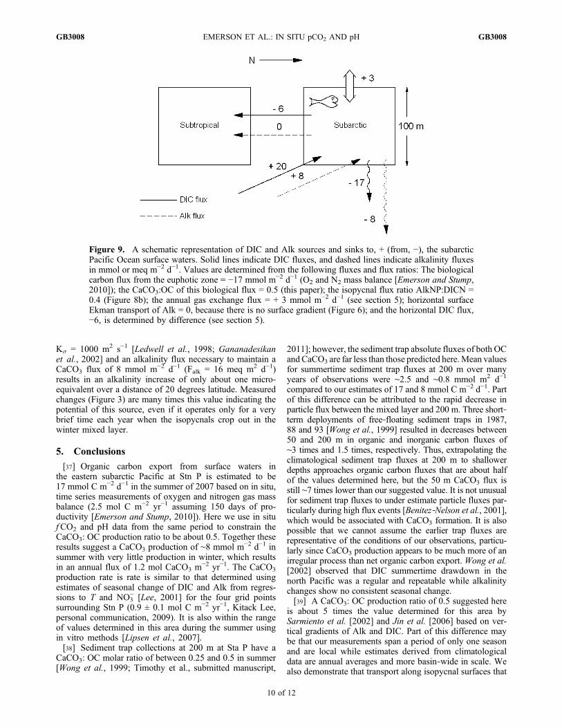
Figure 9. A schematic representation of DIC and Alk sources and sinks to, + (from, −), the subarcticPacific Ocean surface waters. Solid lines indicate DIC fluxes, and dashed lines indicate alkalinity fluxesin mmol or meq m−2 d−1. Values are determined from the following fluxes and flux ratios: The biologicalcarbon flux from the euphotic zone = −17 mmol m−2 d−1 (O2 and N2 mass balance [Emerson and Stump,2010]); the CaCO3:OC of this biological flux = 0.5 (this paper); the isopycnal flux ratio AlkNP:DICN =0.4 (Figure 8b); the annual gas exchange flux = + 3 mmol m−2 d−1 (see section 5); horizontal surfaceEkman transport of Alk = 0, because there is no surface gradient (Figure 6); and the horizontal DIC flux,−6, is determined by difference (see section 5).

EMERSON ET AL.: IN SITU pCO2 AND pH GB3008GB3008

10 of 12

outcrop in the north Pacific is the most important fluxpathway supplying alkalinity to the euphotic zone toaccommodate CaCO3 export determined from our in situmeasurements. Interpreting vertical gradients of Alk andDIC can give misleading results about the importance ofCaCO3 export locally.[40] Using the fluxes reported here we construct a regional

carbon flux balance (Figure 9) that assumes a steady state overa period of at least several years. The net biological organicmatter production of 17 mol m−2 d−1 (2.5 mol C m−2 yr−1)determined from the in situ O2 and N2 measurementscombined with a CaCO3: OC ratio of 0.5 require an alka-linity export of ∼8 meq m−2 d−1 (1.2 mol CaCO3 m

−2 yr−1).The alkalinity that leaves the euphotic zone by biologicalprocesses must be balanced by an isopycnal flux because ofthe very small gradients in normalized potential alkalinity inboth surface waters (Figure 6) and vertically (Figure 8a). Aflux of 8 meq m−2 d−1 of alkalinity to the upper oceanalong isopycnal surfaces with an AlkNP: DICN ratio of0.4 implies an additional source of DIC of ∼20 mmol m−2d−1.The DIC mass balance is closed by a net export of3 mmol m−2 d−1 out of the subarctic upper ocean via thecombined fluxes across the air‐water interface and surfacewater transport to the subtropical ocean.[41] The importance of gas exchange in the carbon cycle

in the northeast subarctic Pacific is determined usingequation (4) and the fCO2 data (Figure 2). To a firstapproximation surface waters were slightly supersaturated inthe summer of 2007, and undersaturated by an average of15 ppm in winter. Using mean gas exchange mass transfercoefficients for CO2 in summer and winter of 3 and 6 m d−1,respectively [see Emerson and Stump, 2010] along withthe f CO2 data results in a mean annual flux from theatmosphere to the ocean of ∼3 mmol m−2 d−1. This addi-tional source to the subarctic mixed layer means that the fluxof DIC to the south via surface ocean advection must beabout 6 mmol C m−2 d−1. Sasai and Ikeda [2003] modeledthe observed DIC distribution in the North Pacific Oceanusing an ocean GCM and climatological distributions ofDIC. Their biological organic carbon export values wereabout half those suggested here and the Ekman transport tothe subtropics was less, but the same fluxes dominated thebalance.[42] The source of alkalinity to the subarctic Pacific

Ocean is from depths of 300–500 m in the subtropicalocean. The carbonate ion concentration necessary for ther-modynamic saturation with respect to aragonite in thesewaters is about 80 mmol kg−1 (Figure 3). Density contoursthat surface above 100 m in the subarctic Pacific in winter(s� = 26.0–26.4, Figure 3) are supersaturated and the degreeof supersaturation actually increases as the isopycnal sur-faces deepen to the south. At steady state there must be asource of alkalinity from CaCO3 dissolution to balance theflux of particulate CaCO3 from the surface waters. From athermodynamic point of view, there is no reason to expectCaCO3 dissolution on density surfaces that supply alkalinityto the subarctic surface waters. The alkalinity source mustcome from either dissolution within undersaturated micro-environments of supersaturated water primarily in the sub-tropical ocean or via mixing of waters containingdissolution‐derived alkalinity from depth [Friis et al., 2006].

[43] Acknowledgments. Ship time for the mooring operations wasprovided by the P‐Line Program of the Institute of Ocean Sciences(IOS), Sidney, B. C., Canada. The authors thank Marie Robert, the Captainand crew of the CCGS Tully, and the IOS administration for collaborationand maintaining an excellent time series program. Charles Stump, PatrickA’Hearn, and David Zimmerman provided outstanding technical help duringthe deployment and recovery of the mooring. We would like to thank DavidTimothy of IOS for showing us a preliminary version of the sediment trappaper compilation and for helpful discussions about the comparison of theirdata with our observations. The research was funded by NSF grants OCE‐0628663 (S.E. and M.C.) and OCE‐0836807 (M.D. and S.C.).

ReferencesArcher, D., S. Emerson, T. Powell, and C. S. Wong (1993), Numericalhindcasting of sea surface pCO2 at Weathership Station Papa, Prog.Oceanogr., 32, 319–351, doi:10.1016/0079-6611(93)90019-A.

Armstrong, R. A., C. Lee, J. I. Hedges, S. Honjo, and S. Wakeham (2002),A new, mechanistic model for organic carbon fluxes in the ocean basedon the quantitative association of POC with ballast minerals, Deep SeaRes., Part II, 49, 210–236.

Ayers, J.M., andM. S. Lozier (2010), Physical controls on the seasonal migra-tion of the North Pacific transition zone chlorophyll front, J. Geophys. Res.,115, C05001, doi:10.1029/2009JC005596.

Balch, W., D. Drapeau, B. Bowler, and E. Booth (2007), Prediction ofpelagic calcification rates using satellite measurements, Deep Sea Res.,Part II, 54, 478–495, doi:10.1016/j.dsr2.2006.12.006.

Benitez‐Nelson, C., K. O. Buesseler, D. M. Karl, and J. Andrews(2001), A time‐series of particulate matter export in the North Pacificsubtropical gyre based on 234Th:238U disequilibrium, Deep Sea Res.,48, 2595–2611, doi:10.1016/S0967-0637(01)00032-2.

Berelson, W. M., W. M. Balch, R. Najjar, R. A. Feely, C. Sabine, and K. Lee(2007), Relating estimates of CaCO3 production, export, and dissolutionin the water column to measurements of CaCO3 rain into sediment trapsand dissolution on the sea floor: A revised global carbonate budget,Global Biogeochem. Cycles, 21, GB1024, doi:10.1029/2006GB002803.

Broecker, W. S., and T. H. Peng (1982), Tracers in the Sea, Eldigio Press,Palisades, N. Y.

Cullison Gray, S. E., M. D. DeGrandpre, T. M. Moore, T. R. Martz,G. E. Friederich, andK. S. Johnson (2011), Applications of in situ pHmea-surements for inorganic carbon calculations, Mar. Chem., 124, 82–90,doi:10.1016/j.marchem.2011.2.005.

Dickson, A. G., J. D. Afghan, and G. C. Anderson (2003), Referencesmaterials for oceanic CO2 analysis: 2. A method for the certification oftotal alkalinity, Mar. Chem., 80, 185–197, doi:10.1016/S0304-4203(02)00133-0.

Emerson, S., and J. H. Hedges (2008), Chemical Oceanography and theCarbon Cycle, Cambridge Univ. Press, Cambridge, U. K., doi:10.1017/CBO9780511793202.

Emerson, S., and C. Stump (2010), Net biological oxygen production in theocean: II. Remote in situ measurements of O2 and N2 in subarctic Pacificsurface waters, Deep Sea Res., Part I, doi:10.1016/j.dsr.2010.06.001.

Favorite, F., J. Dodimead, and K. Nash (1976), Oceanography of the sub-arctic Pacific region, 1960–1971, Int. North Pac. Fish Comm. Bull., 33,187 pp.

Feely, R. A., et al. (2002), In situ calcium carbonate dissolution in thePacific Ocean, Global Biogeochem. Cycles, 16(4), 1144, doi:10.1029/2002GB001866.

Friederich, G. E., P. G. Brewer, R. Herlein, and F. P. Chavez (1995), Mea-surement of sea surface partial pressure of CO2 from a moored buoy,DeepSea Res., Part I, 42, 1175–1186, doi:10.1016/0967-0637(95)00044-7.

Friis, K., R. G. Najjar, M. J. Follows and S. Dutkiewicz (2006), Possibleoverestimation of shallow‐depth calcium carbonate dissolution in theocean, Global Biogeochem. Cycles, 20, GB4019, doi:10.1029/2006GB002727.

Gananadesikan, A., R. D. Slater, N. Gruber, and J. L. Sarmiento (2002),Oceanic vertical exchange and new production: A comparison betweenmodels and observations, Deep Sea Res., Part II, 49, 363–401.

Gregg, M. C. (1989), Scaling turbulent dissipation in the thermocline,J. Geophys. Res., 94, 9686–9698, doi:10.1029/JC094iC07p09686.

Hales, B., and S. Emerson (1997), Calcite dissolution in sediments of theCeara Rise: In situ measurements of porewater O2, pH and CO2,Geochim.Cosmochim. Acta, 61, 501–514, doi:10.1016/S0016-7037(96)00366-3.

Hamme, R. C., and S. R. Emerson (2006), Constraining bubble dynamicsand mixing with dissolved gases: Implications for productivity measure-ments and oxygen mass balance, J. Mar. Res., 64, 73–95, doi:10.1357/002224006776412322.

Hedges, J. I., J. A. Baldock, Y. Gelinas, C. Lee, M. L. Peterson, andS. G. Wakeham (2002), The biochemical and elemental compositions

EMERSON ET AL.: IN SITU pCO2 AND pH GB3008GB3008

11 of 12

of marine plankton: An NMR perspective, Mar. Chem., 78, 47–63,doi:10.1016/S0304-4203(02)00009-9.

Honjo, S., J. Dymond, R. Collier, and S. J. Manganini (1995), Exportproduction of particles to the interior of the equatorial Pacific Ocean during1992 EqPac experiment,Deep Sea Res., Part II, 42, 831–870, doi:10.1016/0967-0645(95)00034-N.

Howard, E., S. Emerson, S. Bushinsky, and C. Stump (2010), The role ofnet community biological production in air‐sea carbon fluxes at theNorth Pacific subarctic‐subtropical transition region, Limnol. Oceanogr.,55, 2585–2596, doi:10.4319/lo.2010.55.6.2585.

Jahnke, R. A., D. B. Craven, and J.‐F. Gaillard (1994), The influence oforganic matter diagenesis on CaCO3 dissolution at the deep‐sea floor,Geochim. Cosmochim. Acta, 58, 2799–2809, doi:10.1016/0016-7037(94)90115-5.

Jin, X., N. Gruber, J. P. Dunne, J. L. Sarmiento, and R. A. Armstrong(2006), Diagnosing the contribution of phytoplankton functional groupsto the production and export of particulate organic carbon, CaCO3, andopal from global nutrient alkalinity distributions, Global Biogeochem.Cycles, 20, GB2015, doi:10.1029/2005GB002532.

Johnson, K. M., et al. (1998), Coulometric total carbon dioxide analysis formarine studies: Assessment of the quality of total inorganic carbon mea-surements made during the U.S. Indian Ocean CO2 survey 1994–1996,Mar. Chem., 63, 21–37, doi:10.1016/S0304-4203(98)00048-6.

Klaas, C. and D. E. Archer (2002), Association of sinking organic matterwith various types of mineral ballast in the deep sea: Implications forthe rain ratio, Global Biogeochem. Cycles, 16(4), 1116, doi:10.1029/2001GB001765.

Kwon, E. Y., F. Primeau, and J. L. Sarmiento (2009), The impact ofremineralization depth on the air‐sea carbon balance, Nat. Geosci., 2,630–635, doi:10.1038/ngeo612.

Large, W. G., J. C. McWilliams, and P. P. Niller (1986), Upper oceanthermal response to strong autumnal forcing of the northeast Pacific,J. Phys. Oceanogr., 16, 1524–1550, doi:10.1175/1520-0485(1986)016<1524:UOTRTS>2.0.CO;2.

Large, W. G., J. C. McWilliams, and S. C. Doney (1994), Oceanic verticalmixing: A review and a model with a nonlocal boundary layer parame-terization, Rev. Geophys., 32, 363–403, doi:10.1029/94RG01872.

Ledwell, J. R., A. J. Wilson, and C. S. Law (1998), Mixing of a tracer in thepycnocline, J. Geophys. Res., 103, 21,499–21,529, doi:10.1029/98JC01738.

Lee, K. (2001), Global net community production estimated from theannual cycle of surface water total dissolved inorganic carbon, Limnol.Oceanogr., 46, 1287–1297, doi:10.4319/lo.2001.46.6.1287.

Lee, K., L. T. Tong, F. J. Millero, C. L. Sabine, A. G. Dickson, C. Goyet,G‐H. Park, R. Wanninkhof, R. A. Feely and R. M. Key (2006), Globalrelationships of total alkalinity with salinity and temperature in surfacewaters of the world’s oceans, Geophys. Res. Lett., 33, L19605,doi:10.1029/2006GL027207.

Lipsen, M. S., D. W. Crawford, J. Gower, and P. J. Harrison (2007), Spatialand temporal variability in coccolithophore abundance in the productionof PIC and POC in the NE subarctic Pacific during El Niño 1998, La Niña1999 and 2000, Prog. Oceanogr., 75, 304–325, doi:10.1016/j.pocean.2007.08.004.

Lueker, T. J., A. G. Dickson, and C.D. Keeling (2000), Ocean pCO2calculated from dissolved inorganic carbon, alkalinity and the equationsfor K1 and K2: Validation based on laboratory measurements of CO2 ingas and seawater at equilibrium, Mar. Chem., 70, 105–119, doi:10.1016/S0304-4203(00)00022-0.

Martz, T. R., J. J. Carr, C. R. French, and M. D. DeGrandpre (2003), Asubmersible autonomous sensor for spectrophotometric pH measure-ments of natural waters, Anal. Chem., 75, 1844–1850, doi:10.1021/ac020568l.

Mehrbach, C., H. Culberson, J. E. Hawley, and R. M. Pytkowicz (1973),Measurement of the apparent dissociation constants of carbonic acid in

seawater at atmospheric pressure, Limnol. Oceanogr., 18, 897–907,doi:10.4319/lo.1973.18.6.0897.

Millero, F. J., et al. (1998), Total alkalinity measurements in the in IndianOcean during the WOCE Hydrographic Program CO2 survey cruises1994–1996,Mar. Chem., 63, 9–20, doi:10.1016/S0304-4203(98)00043-7.

Moore, J. K., S. C. Doney, J. A. Kleypas, D. M. Glover, and I. Y. Fung(2002), An intermediate complexity marine ecosystem model for theglobal domain, Deep Sea Res., Part II, 49(1–3), 403–462.

Mucci, A. (1983), The solubility of calcite and aragonite in seawater atvarious salinities, temperatures, and one atmosphere total pressure,Am. J. Sci., 283, 780–799, doi:10.2475/ajs.283.7.780.

Nightingale, P. D., G. Malin, C. S. Law, A. J. Watson, P. S. Liss,M. I. Liddicoat, J. Boutin, and R. C. Upstill‐Goddard (2000), In situevaluation of air‐sea gas exchange parameterizations using novel conser-vative and volatile tracers, Global Biogeochem. Cycles, 14, 373–387,doi:10.1029/1999GB900091.

Roden, G. (1977), Ocean subarctic fronts of the central Pacific: Structure ofthe response to atmospheric forcing, J. Phys. Oceanogr., 7, 761–778,doi:10.1175/1520-0485(1977)007<0761:OSFOTC>2.0.CO;2.

Sarmiento, J. L., and N. Gruber (2007), Ocean Biogeochemical Dynamics,Princeton Univ. Press, Princeton, N. J.

Sarmiento, R. L., J. Dunne, A. Gnanadesikan, R. M. Key, K. Matsumotoand R. Slater (2002), A new estimate of the CaCO3 to organic carbonexport ratio, Global Biogeochem. Cycles, 16(4), 1107, doi:10.1029/2002GB001919.

Sasai, Y., and M. Ikeda (2003), A model study for the carbon cycle in theupper layer of the North Pacific, Mar. Chem., 81, 71–88.

Seidel, M. P., M. D. DeGrandpre, and A. G. Dickson (2008), A sensor forin situ indicator‐based measurements of seawater pH, Mar. Chem., 109,18–28, doi:10.1016/j.marchem.2007.11.013.

Tabata, S. (1961), Temporal changes of salinity, temperature and dissolved oxy-gen content of the water at Station “P” in the northeast Pacific Ocean, andsome of their determining factors, J. Fish. Res. Bd. Can., 18, 1073–1124,doi:10.1139/f61-066.

Weiss, R. F. (1974), Carbon dioxide in water and seawater, the solubility ofan non‐ideal gas, Mar. Chem., 2, 203–215, doi:10.1016/0304-4203(74)90015-2.

Wong, C. S., and Y.‐H. Chan (1991), Temporal variations in the partialpressure and flux of CO2 at ocean station P in the subarctic northeastPacific Ocean, Tellus, Ser. B, 43, 206–223.

Wong, C. S., F. A. Whitney, D. W. Crawford, K. Iseki, R. J. Matear,W. K. Johnson, J. S. Page, and D. Timothy (1999), Seasonal and inter-annual variability in particle fluxes of carbon, nitrogen and silicon fromtime series sediment traps at Ocean Station P, 1982–1993: Relationshipto changes in subarctic primary productivity, Deep Sea Res., Part II,46, 2735–2760, doi:10.1016/S0967-0645(99)00082-X.

Wong, C. S., D. Waser, Y. Nojiri, F. A. Whitney, J. Page, and J. Zeng(2002), Seasonal cycles of nutrients and dissolved inorganic carbon athigh and mid latitudes in the North Pacific Ocean during the Skaugrancruises: Determination of new production and nutrient uptake ratios,Deep Sea Res., Part II, 49, 5317–5338, doi:10.1016/S0967-0645(02)00193-5.

Yamanaka, Y., and E. Tajika (1996), The role of the vertical fluxes ofparticulate organic matter and calcite in the oceanic carbon cycle: Studiesusing an ocean biogeochemical general circulation model, Global Biogeo-chem. Cycles, 10, 361–382, doi:10.1029/96GB00634.

M. F. Cronin, R. Feely, and C. Sabine, Pacific Marine EnvironmentalLaboratory, NOAA, Seattle, WA 98115, USA.S. E. Cullison Gray and M. DeGrandpre, Department of Chemistry and

Biochemistry, University of Montana, Missoula, MT 59812, USA.S. Emerson, School of Oceanography, University of Washington, Seattle,

WA 98195, USA. (emerson@u.washington.edu)

EMERSON ET AL.: IN SITU pCO2 AND pH GB3008GB3008

12 of 12