Embed Size (px)
Citation preview

Global Agri-Food Export Competitiveness By Štefan Bojnec
1 and Imre Fertő
2,
1University of Primorska
2Institute of Economics, Hungarian Academy of Sciences and Corvinus University of Budapest
The article investigates agri-food export competitiveness of 23 countries on global
markets using revealed comparative advantage (B) index in the 2000-2011 periods.
Results indicate that main global agri-food exporting countries have revealed
comparative advantages. The panel unit root tests suggest convergence in the
dynamics of the B indices. Mobility indices indicate relatively low mobility in the B
indices at the product level. The Kaplan-Meier survival rates of the B indices on long-
term are among the highest for the Netherlands, France, Belgium, the United States,
Argentina and New Zealand. The level of economic development, the share of
agricultural employment, subsidies to agriculture, and differentiated consumer agri-
food products increases the likelihood of failure in comparative advantage, while
agricultural land abundance and export diversification reduces.
Keywords: global agri-food export – revealed comparative advantage – panel unit root tests – intra-
distribution dynamics – duration analysis – discrete time models
JEL codes: F01, F14, C23, C41, Q17

1. Introduction
With trade liberalization on global agri-food markets, the crucial factor for long-term business
survival is export competitiveness and its long-term duration, which determines opportunities in
the business prosperity of agri-food products on global markets. On the global agri-food markets,
different countries play the role of global leaders in agri-food export competitiveness. So far,
there has been limited attention to the agri-food export competitiveness and long-term export
specialisation patterns of global agri-food leaders. On global agri-food markets, can be observed
three main stylized empirical facts, which are important for research and practice on global
businesses (European Commission, 2012, 2013; WTO, 2013; FAO, 2014). First, during the last
two decades of agri-food trade liberalization, global agri-food export has increased rapidly,
particularly due to fast growth in processed and final consumer agri-food products. Global agri-
food exports tend to increase in response to food demand increases. Some variations with a
contraction in global agri-food export have been caused by the impact of the economic crisis in
2009, exchange rate and global price fluctuations by countries and by agri-food products.
Second, the increase in global agri-food export has been both from developed and developing
countries. Among the global leading agri-food exporters are France, Germany, the Netherlands,
and Belgium in the European Union (EU), the United States (US) and Brazil. Developed
countries are substantial exporter of final products, which have become the most important in the
structure of global agri-food trade. Third, the EU is the global biggest importer of agricultural
products from developing countries, followed by China's fast growth in imports, and Japan as the
third largest importer. The US, Russia, and China (including Hong Kong) are the top EU's
biggest agri-food markets (FAO, 2014).
The aim of the paper is to examine the pattern, stability and determinants of global agri-food
export competitiveness of major agri-food exporter and importer countries at the global markets.
Considering the global stylized empirical facts, the objective of this paper is to provide empirical
evidence and derives explanation on the following four research questions. First, the most recent
structures and dynamics of agri-food exports and the magnitude and dynamics of revealed
comparative advantage (B) index by major global competitors. Second, the analysis of stability

of the B indices using panel unit root tests of the null hypothesis on the existence of the panel
unit root (divergence) or the alternative hypothesis of the stationarity of panel datasets
(convergence to their equilibrium state) using a variety of panel unit root tests. Third, long-term
export specialization patterns, duration analysis and intra-distribution dynamics of B indices
using Markov transition probability matrices and nonparametric Kaplan-Meier product limit
estimator. Fourth, main driving forces of global agri-food export competiveness using discrete
time models. The econometric models test the set hypotheses and explain the determinants of the
B index considering structural nature and dynamic aspects of an economy, factor endowments in
agriculture and policy support to agriculture.
2. Background
Agri-food export-oriented growth is largely based on processed agri-food products from
developed countries and less from non-traditional agricultural exports from developing countries
(Patel-Campillo, 2010). Our sample contains 23 countries including the four major agri-food
exporting countries in the EU (France, Germany, the Netherlands, and Belgium) (e.g. Bojnec and
Fertő, 2015), BRICS-5 countries (Brazil, Russia, India, China and South Africa) as an
association of five major emerging fast-growing economies, the North American Free Trade
Agreement (NAFTA-3) countries (Canada, Mexico, and the US), the MIST-4 countries (Mexico,
Indonesia, South Korea, and Turkey), Tiger Cup-4 countries (Indonesia, Malaysia, the
Philippines, and Thailand) as the four newly industrialized countries, and selected global major
agri-food trading countries such as Argentina, Australia and New Zealand in global agri-food
exports and Japan and Switzerland in global agri-food imports (European Commission, 2013).
The BRICS-5 represents the world largest size of territory and population. They represent one of
largest world economies in terms of agri-food production and consumption. The NAFTA-3 is
one of the world largest trade blocs according to the economic size or by the size of gross
domestic product (GDP). The Tiger Cub-4 countries follow the export-driven model of rapid
growth and economic development with a bamboo network of overseas Chinese businesses
operating that share common family and cultural ties. When focusing on major global trading
groups of countries, there are some overlaps and double counting issues as some countries are

members of more than a single trading group of countries such as Mexico in NAFTA-3 and
MIST-4, and Indonesia in MIST-4 and Tiger Cup-4. This is the reason that the focus of the
analysis and the presentation of the results is on the levels and trends in the B indices as a
measure of export specialization by the individual countries and less by main trading groups.
The stylized empirical facts indicate that the EU experienced the largest agricultural trade
surplus being the second largest agricultural exporter immediately behind the US in the ranking
of global top agricultural exporters (European Commission, 2013). Exports markets particularly
in developing economies such as in China and Saudi Arabia are crucial for the growth in demand
for EU agri-food exports.
3. Methodology
The country’s i agri-food export share in total global agri-food exports is calculated as:
where Xi% is in the share (in per cent) of the value of agri-food export Xi of the county’s i in total
global value of agri-food exports , where n is the number of countries in the world.
The country’s i agri-food import share in total global agri-food imports is calculated as:
where Mi% is in the share (in per cent) of the value of agri-food import Mi of the county’s i in
total global value of agri-food imports , where n is the number of countries in the world.
The paper employees the concept of ‘revealed’ comparative advantage introduced by Liesner
(1958) and later redefined and popularized by Balassa (1965). Therefore, it is known as the
‘Balassa index’ to empirically identify a country’s weak and strong export sectors. The Revealed
Comparative Advantage (B) index is defined (Balassa, 1965) as follows:
B = (Xij / Xit) / (Xnj / Xnt) ,

where X represents exports, i is a country, j is a commodity, t is a set of commodities, and n is a
set of countries, which are used as the benchmark export markets for comparisons. B is based on
observed export patterns. In this paper, the B index is calculated at the 6-digit level of the World
Customs Organization’s Harmonized System (HS-6). It measures a country’s exports of a
commodity relative to its total exports and to the corresponding export performance of a set of
countries, e.g., the global agri-food exports. If B > 1, then a country’s agri-food comparative
export advantage on the global market is revealed. In a spite of some critics of the B index as
export specialisation index, such as the asymmetric value problem and problem with logarithmic
transformation (De Benedictis and Tamberi, 2004) and the importance of simultaneous
consideration of the import side (Vollrath, 1991), it can provide useful evidence on the country’s
agri-food export competitiveness on global markets.
In addition, we focus on the stability of the B indices over time. The first type of stability of the
distribution of the B indices is capturing convergence/divergence in revealed comparative export
advantage. Time series investigation of the convergence hypothesis in economic literature often
relies on unit root tests. The rejection of the null hypothesis is commonly interpreted as evidence
that the time series have converged to their equilibrium state, since any shock that causes
deviations from equilibrium eventually drops out. To check convergences or divergence in the B
indices, three panel unit root tests with and without trend specifications, respectively, as a
deterministic component are used: Im et al. (2003) method (assuming individual unit root
processes), ADF–Fisher Chi–square, and PP–Fisher Chi–square (Maddala and Wu, 1999; Choi,
2001). In addition, the lag length of explanatory variables has been chosen according to the
Modified Akaike Information Criterion (MAIC) proposed by Ng and Perron (2001).
The second type of stability of the value of the B indices for particular agri-food product groups
is investigated in two steps. First, we employ Markov transition probability matrices to identify
the persistence and mobility of B indices. We classify agri-food products into two categories:
agri-food products with revealed comparative export disadvantage (B<1) and agri-food products
with revealed comparative export advantage (B>1). Second, the degree of mobility in patterns of
revealed comparative export advantage can be summarised using an index of mobility. This

formally evaluates the degree of mobility throughout the entire distribution of B indices and
facilitates direct cross-country comparisons. The mobility index M1, following Shorrocks (1978)
evaluates the trace (tr) of the Markov transition probability matrix. This M1 index thus directly
captures the relative magnitude of diagonal and off-diagonal terms, and can be shown to equal
the inverse of the harmonic mean of the expected duration of remaining in a given cell:
1K
)P(trK
1M
,
where K is the number of groups, and P is the Markov transition probability matrix. A higher
value of M1 index indicates greater mobility (the upper limit is two in our case), with a value of
zero indicating perfect immobility.
Duration analysis of revealed comparative export advantage (B>1) is estimated by the survival
function, S(t), using the nonparametric Kaplan-Meier product limit estimator (Cleves et al.,
2004). We assume that a sample contains n independent observations denoted (ti; ci), where i = 1,
2,…, n, ti is the survival time, and ci is the censoring indicator variable C taking a value of 1 if
failure occurred, and 0 otherwise of observation i. It is assumed that there are m < n recorded
times of failure. The rank-ordered survival times are denoted as t(1) < t(2) < … < t(m), while nj
denotes the number of subjects at risk of failing at t(j), and dj denotes the number of observed
failures. The Kaplan-Meier estimator of the survival function is then:
j
jj
tit n
dntS
)(
)(ˆ ,
with the convention that 1)(ˆ tS if t < t(1). Given that many observations are censored, it is then
noted that the Kaplan-Meier estimator is robust to censoring and uses information from both
censored and non-censored observations.
Beyond to descriptive analysis of duration of revealed comparative advantage we are interesting
for the factors explaining the survival. Recent literature on the determinants of trade and
comparative advantage duration uses Cox proportional hazards models (e.g. Besedeš and Prusa,
2006b; Nitsch, 2009; Brenton et al., 2010; Obashi, 2010; Bojnec and Fertő, 2012b; Cadot et al.,
2013). However, recent papers point out three relevant problems inherent in the Cox model that

reduce the efficiency of estimators (Brenton et al., 2010; Hess and Persson, 2011, 2012). First,
continuous-time models (such as the Cox model) may result in biased coefficients when the
database refers to discrete-time intervals (years in our case) and especially in samples with a high
number of ties (numerous short spell lengths). Second, Cox models do not control for
unobserved heterogeneity (or frailty). Thus, results might not only be biased, but also spurious.
The third issue based on the proportional hazards assumption that implies similar effects at
different moments of the duration spell. Following Hess and Persson (2011) we estimate
different discrete-time models including probit and logit specifications, where product-exporter
country random effects are incorporated to control for unobservable heterogeneity.
The challenging issues for firms and countries are to strengthen determinants of the duration of
comparative advantages as well as transform disadvantages into advantages in international trade
(e.g. Contractor et al., 2007; Cuervo-Cazurra and Genc, 2008). Following the previous research
on trade and comparative advantage duration we test the following hypotheses.
Exports can be positively sensitive to level of economic development, which is proxied by per
capita gross domestic product (GDP) of exporting countries. Therefore, the duration of
comparative advantage is positively associated to the level of economic development. A positive
relation between product differentiation and per-capita GDP sensitivity is consistent with
hypothesis on preferences of consumers for quality and demand for varieties with higher level of
economic development (e.g. Philippidis and Hubbard, 2003; Hallak, 2006; Choi et al. 2009).
H1: Duration of comparative advantage is positively associated with the level of economic
development.
The size of the economy can be measured by the size of GDP and/or by the size of population
(e.g. Helpman, 1998). The size of the economy is traditional gravity trade model variable with
expected positive association between bilateral exports and the size of economy (e.g. Anderson
and van Vincoop, 2003). We expect that larger countries tend to have comparative advantage for
longer period than smaller ones. The population differential increases between the regions
increases exports.

H2: Larger countries tend to have comparative advantage of longer duration than smaller ones.
A large part of agricultural production depends on natural agricultural factor endowments.
Among them a crucial role can play availability and quality of land soil potentials and natural
climatic conditions. Better endowment in agricultural resources can through more competitive
agricultural production also increase competitiveness of food processing industry and thus of
agri-food comparative advantages.
H3: Better endowment in agricultural resources increase the probability of survival of
comparative advantage.
When modelling export duration for final products within a sector, the assumption of product
homogeneity is often quite unrealistic due to different varieties of the product and its
considerable heterogeneity (e.g. Helpman and Krugman, 1985). Countries with a generally
diversified export structure will have a more chance to have comparative advantage in a given
product for long periods of time (Nitsch, 2009; Hess and Persson, 2011). For agri-food products,
we assume that more product heterogeneity exists in value chain according to the degree of
product processing. Heterogeneity between vertical stages in value chain is related to the
processing of primary agricultural products either for further processing or for final human
consumption. In addition, the duration of comparative advantage is expected to be of longer
duration for differentiated agri-food products than homogeneous ones (Rauch and Watson, 2003;
Besedeš and Prusa, 2006).
H4: Export diversification has positive impact on duration of comparative advantage in a given
agri-food product and the duration of comparative advantage is longer for differentiated agri-
food products than homogeneous ones.
The literature on political economy of agricultural policy and government transfers emphasise
the negative relationships between agricultural subsidies and comparative advantage (e.g.
Anderson et al., 2013).
H5: Agricultural support has negative impact on survival of comparative advantage.

4. Data
The United Nations (UN) International Trade Statistics UN Comtrade database (UNSD, 2013) at
the six-digit harmonized commodity description and coding systems (HS6-1996) level is used for
agri-food exports by the leading agri-food exporting and trading groups of countries on global
agri-food markets. Agri-food trade defined by the World Trade Organization contains 789 HS-6
level product groups. The UN Comtrade database with the World Integrated Trade Solution
(WITS) software developed by the World Bank, in close collaboration and consultation with
various international organizations including United Nations Conference on Trade and
Development (UNCTAD), International Trade Center (ITC), United Nations Statistical Division
(UNSD) and WTO is used. The value of trade is expressed in US dollars.
The proxy for economic development is the log of GDP per capita at purchasing power parity
(PPP) at constant 2005 international US dollars based on the World Bank (2013b). The logarithm
of the populations of exporter country is used as a proxy for the market size. Population data are
also from the World Bank (2013b).
We use two proxies for agricultural factor endowments: first, the share of agricultural land in
total land, and second, the share of active agricultural employment in total active employment.
Land data is based on the World Bank (2013b), while agricultural employment data taken from
the FAO (2014) database.
The agri-food export diversification is measured by natural logarithm of the number of agri-food
exported products per year. We define a dummy for the differentiated agri-food products as
consumption or final agri-food products based on the UN classification by Broad Economic
Categories (BEC). For agri-food items final goods are described by two BEC categories: BEC
112 – primary agricultural products mainly for household consumption and BEC 122 –
processed agri-food products mainly for household consumption. The primary source of data for
export diversification (the number of exported agri-food products) and consumer (differentiated)
agri-food products is UNSD (2013).

We use the Nominal Rate of Assistance (NRA) to measure the agricultural supports based on the
World Bank (2013a). Positive values of the NRA indicate protection to agricultural sectors,
whilst negative values mean its taxation.
Dependent and all explanatory variables in the panel are capturing each of the EU-27 member
states in the twelve year analyzed (2000-2011).
5. Empirical results
5.1. Countries Shares in Global Agri-Food Exports and Imports
According to the agri-food export and import shares in the global markets, the analyzed countries
have been net exporters, because their overall share in global agri-food exports was higher than
their overall import share in global agri-food imports (Figure 1). The import share has declined
from more to less than 60 per cent during the analysed period, while export share has remained
close to 70 per cent. The share of gross trade is ranging around 65 per cent.
Figure 2 compares the global market agri-food export and import shares of individual analyzed
countries in the years 2000 and 2011. In 2011, the major agri-food exporters are the United
States (US), the Netherlands, Germany, Brazil and France. Comparisons between 2000 and 2011
show a rapid increase in agri-food export share for Brazil, and deterioration for France and
Belgium. In 2011, the major agri-food importers are the United States, Germany, China, Japan,
the Netherlands and France. Comparisons between 2000 and 2011 show a rapid increase in agri-
food import share for China. This is consistent with the previous findings in the literature (e.g.
Bojnec et al., 2014).
5.2. Changes in Revealed Comparative Advantage (B) Indices
According to the distribution of the mean and median values of the B indices and for the
percentage of agri-food products with the B>1, the agri-food B indices suggest that export
competitive countries on the global markets are: Argentina, Australia, Belgium, France, the
Netherlands, New Zealand, and the US (Figure 3). They experienced: the B mean values greater

than 1 (B>1), the higher B median values, and the increasing or stable percentage of agri-food
products with the B>1, which is greater than 30%. With lower share of the B>1 are close to this
group also Turkey and Canada. The Netherlands has further improved export competitiveness,
while it has deteriorated a slightly for Australia and Turkey.
The second group according to the B indices are mostly the BRICS and MIST countries with the
revealed comparative advantage or the B mean value greater than 1 (B>1), but with rather
diversified median values and the lower percentage of agri-food products with the B>1: Brazil,
India, South Africa, Indonesia, Malaysia, Philippines, Thailand, and to a lesser extent China,
which experienced deterioration of revealed comparative advantage from advantage B>1 in 2000
to disadvantage B<1 in 2011. Some deterioration in export competitiveness is also for India,
while improvements for Philippines.
The third group with revealed comparative disadvantage (B<1) consists of the four countries
with the lowest B mean value less than one (B<1), the lowest B median value, and the share with
the B>1 less than 10%; these are: Russia, Japan, South Korea, and Switzerland.
Finally, the fourth group consists of Germany and Mexico with revealed comparative
disadvantage (B<1), with lower (Mexico) to medium (Germany) value of the B median value,
and the share with the B>1 close or more than 19%. Germany has slightly improved export
competitiveness.
Except for Russia and China with annual variation, the BRICS countries have experienced the
B>1 for agri-food exports on the global markets. Among the NAFTA countries, only the USA is
clearly performed with revealed comparative advantage (B>1) for agri-food products. The MIST
countries in general experienced revealed comparative advantage (B>1). Among the Tiger Cup
countries, Philippines have the highest values for the B>1 indices.
Except for the Netherlands, France, Belgium, the US and to a lesser extent for Argentina, the
median values are lower suggesting the greater number of agri-food products with revealed

comparative disadvantages (B<1) vis-à-vis revealed comparative advantages (B>1) on the global
markets. This implies that the global agri-food exports by competitiveness are clearly dispersed
among different countries’ players by different agri-food products, which can be explained by
different sources of revealed comparative advantages and export specialisation patterns from
natural factor endowments and climatic conditions to development of agri-food processing
industries and international agri-food marketing as well as some other countries specific factors.
5.3. Dynamics of the B Indices
To investigate convergence vis-à-vis divergence in the dynamics of the B indices, panel unit root
tests with time-trend and without time-trend specifications, respectively, as a deterministic
component are used (Table 1). The empirical results of the three different panel unit root tests
without time-trend clearly reject the existence of the panel unit root hypothesis for all countries.
This implies that the B indices are stationary confirming the hypothesis of convergence in the
dynamics of the B indices.
5.4. Mobility of the Revealed Comparative Advantage
The degree of mobility in patterns throughout the entire distribution of the B indices is estimated
using the mobility index, M1, based on the Markov transition probability matrices using a one
year lag. The empirical results in Figure 4 indicate relatively low mobility in the B indices at the
HS-6 product level by the analysed countries. Except for India, Russia, and South Africa, the M1
indices on average for agri-food products by the analysed countries are less than 0.2 indicating
rather high stability with relatively low mobility in patterns of the B indices for agri-food
products. Except for Malaysia and to a lesser extent for Mexico, the degree of mobility in the B
indices is a slightly higher for non-consumer agri-food products than for consumer agri-food
products. This finding indicates a relatively low degree of mobility and thus relatively high
stability in patterns throughout the entire distribution of the B indices at the HS-6 agri-food
product level by the analyzed countries.

5.5. Duration of the Revealed Comparative Advantage (B>1) Indices
The duration of the B>1 indices is investigated in two steps: first, the duration of B>1 in the
years during the analyzed period, and second, the description of the periods of time as a
continuous process (or ‘spells’) of B>1. The former indicates for how many years B>1 at the HS-
6 agri-food product levels, ranging from 1 to 12 years during the 12-years analyzed period. The
latter indicates whether the B>1 is a continuous process during the analysed period as a whole
with a single spell or with multiple spells up to six with switches year-to-year ins and outs from
B>1 to B<1 during the 12-years analyzed period.
Figure 5 presents the results of the duration analysis of the B>1 indices for the HS-6 number of
agri-food products. The highest average number of years with the B>1 duration are for France,
New Zealand, Japan, the US, Australia and Argentina. The number of the HS-6 agri-food
products with B>1 over the 12-years duration is the largest for the Netherlands, whilst the mean
and median values of the B>1 duration are the highest for France. In general, the average number
of years with the B>1 duration is greater for the consumer HS-6 agri-food products than for the
non-consumer HS-6 agri-food products, which is consistent with the set H 4.
A single agri-food product can change its B>1 position to B<1 year-to-year, e.g. six times within
the 12-years analyzed period. Six is the maximum possible number of spells when an agri-food
product has changed its B>1 status year-to-year. The analyzed number of spells for the HS-6
agri-food products B>1 indices by the analysed spell length years show the number of
relationships that are characterized by the single and multiple spells for the HS-6 agri-food
products B>1 indices by the analysed countries on the global markets. Around three-quarters of
the spells are concentrated in the single spell (Figure 6). This finding indicates that most of the
HS-6 agri-food products export competitiveness failed after the first or shorter number of years.
The distribution of the number of spells for the HS-6 agri-food products with B>1 indices that
survived continuously at least a single year up to twelve years vary from one single spell up to
five multiple spells. Japan has the greatest percentage of agri-food products with B>1 as the
single spell and India has the lowest percentage.
5.6. Survival of the Revealed Comparative Advantage (B>1) Indices
The duration of the mean values of the B>1 indices for agri-food exports by the analysed
countries on the global market is tested by examining nonparametric Kaplan-Meier estimates of
a survival function over the 12-year analyzed periods. The mean values for countries with higher
B>1 indices for the HS-6 agri-food products exports are expected to be of longer duration. The
Kaplan-Meier survival rates for the mean values of the B>1 indices by each of the analysed
country have declined over time (Figure 7).
The duration of the mean values of the B>1 indices over the 12-year periods differs between the
analyzed countries and can be divided in three groups. First, the highest survival rates are found
for the Netherlands, France, Belgium, Argentina, the US, and New Zealand. The higher survival
rates over time imply their relatively higher ability to maintain the B>1 indices with revealed
comparative advantages on long-term.
Second, the modest Kaplan-Meier survival rates around 5% over the 12-year period are found for
the following countries: Germany, Turkey, Canada, and Australia. In addition, in this group of
countries to a lesser extent can be included the following analyzed countries with the Kaplan-
Meier survival rates more than 3% over the 12-year period: India, Brazil, South Africa,
Indonesia, Philippines, and Thailand.
Third, the Kaplan-Meier survival rates are relatively low (less than 3% after 12 years analysed
period) for the following countries: China, Russia, Mexico, Japan, South Korea, Switzerland, and
Malaysia. The results for this group of the analysed countries imply that the duration of their
agri-food exports on the global markets is shorter and their probability of survival is lower.
These countries can have some specific agri-food products, which can have higher B>1 indices
with longer duration and higher survival rate such as for some niche agri-food products.
However, they are less likely to maintain competitive their agri-food exports for a larger number
of agri-food products on the global markets on long-term.

The results of the duration of the mean values of the B>indices over the 12-year periods are
mixed between consumer and non-consumer agri-food products. First, no substantial differences
in the Kaplan-Meier survival rates can be seen for Japan, South Korea, Switzerland, China,
South Africa, and Thailand. Most of these countries belong to a group of countries with
relatively low survival rates. Second, the Kaplan-Meier survival rates are higher for consumer
agri-food products than non-consumer agri-food products: the Netherlands, France, Bulgaria,
New Zealand, Turkey, and Mexico. This finding is consistent with the set H4. Third, the Kaplan-
Meier survival rates are higher for non-consumer agri-food products than consumer agri-food
products: Argentina, the US, Germany, Canada, Australia, India, Brazil, Indonesia, Philippines,
Malaysia, and Russia. These mixed findings suggest specificities of determinants explaining the
duration of export competitiveness in different global agri-food net exporting/importing
countries.
5.7. Explanation of the Duration of Revealed Comparative Advantage (B>1) Indices
We estimate the baseline specification using discrete-time probit and logit models, which are
then additionally specified with consumer agri-food products dummy variable (Table 2). All
models include random effects for every exporter-product combination.
In general, the sign of coefficients are similar for the various estimation procedures. We find the
larger log-likelihood value for the logit models comparing to probit models. The values of rho
mean that random effect explains around 95 per cent of unobserved heterogeneity in all
specifications. The likelihood-ratio tests strongly reject the null hypothesis of no latent
heterogeneity for all model specifications, confirming that unobserved heterogeneity plays a
significant role in all model specifications.
The GDP per capita has a positive and significant coefficients, suggesting that comparative
advantage involving economically developed economy increases the likelihood of failure in the
B>1 indices. The market size in terms of the size population has no significant impacts on the
likelihood of failure in the B>1 indices. The two factor endowment variables have opposite
effects on the likelihood of failure in the B>1 indices. The B>1 indices in land abundant

countries have more chance to survive as this decreases the probability of failure in the B>1
indices, whilst more agricultural employment increases the likelihood of failure in the B>1
indices. The significant negative regression coefficients on the number of agri-food exported
products indicate that exporting many products decreases the likelihood of failure in the B>1
indices. We find that agricultural supports increases the probability of failure in the B>1 indices.
Contrary to the theoretical predictions by Rauch and Watson (2003), we find that the B>1 indices
in differentiated consumer agri-food products will have a larger likelihood of failure.
To sum up the findings regarding the set hypotheses on the likelihood of failure in the B>1
indices, we reject the H1, because the higher level of economic development is not confirmed to
reduces the probability of failure in the B>1 indices. The results for the set H2 are not found
statistically significant. The results for the set H3 are mixed: we cannot reject the association
with the land abundant variable, while the association with agricultural population is rejected.
The results for the set H4 are also mixed: we cannot reject the association with the export
diversification, while the association with the differentiated consumer agri-food products is
rejected. Finally, we cannot reject the set H5 as agricultural support increases the likelihood of
failure in the B>1 indices.
6. Conclusions
The article investigates agri-food export competitiveness on global markets for 23 major
countries accounting more than 60 percent of global agri-food trade. Most of the analyzed
countries have been competitive in agri-food exports with revealed comparative advantage (B>1)
on global markets. Export specialisation by countries is on a smaller number of the HS-6 agri-
food products with revealed comparative advantage (B>1).
The convergences in the dynamics of the B indices further reinforced findings on similar global
competitive pressures on long-term specialisation patterns and survival rates of competitive agri-
food products. The switches in revealed comparative advantages between agri-food products
over time are found relatively low, which implies that the focus in agri-food export specialisation

patterns is on existing established or niche agri-food products, which are able to survive global
competition on long-term.
The number of the HS-6 agri-food products with revealed comparative advantages (B>1) and
their survival rates make the major differences between the global players in agri-food export
competitiveness. Higher B>1 indices, larger number of the HS-6 agri-food products with B>1
with the longer duration and higher survival rates are found for the Netherlands, France, Belgium
and some overseas countries from different parts of the world, particularly Argentina, the US,
and New Zealand.
The regression results of probit and logit models are mixed. As expected, agricultural land
abundance and export diversification reduces the likelihood of failure in the B>1 indices, while
agricultural subsidies increases. Unlike to our expectation, the level of economic development,
the share of agricultural employment, and differentiated consumer agri-food products increases
and not reduces the likelihood of failure in the B>1 indices. Yet, the regression coefficient for the
population size is not found statistically significant. These results suggest substantial
heterogeneity between agri-food competitors on global markets. Finally, the empirical findings
suggest that there are also numerous other non-analyzed countries, particularly developing ones,
which can have greater difficulties in agri-food export competitiveness, particularly for non-
primary raw agricultural and low processed food products. These are issues for future research in
order to widen and deepen our knowledge and better understanding of global agri-food export
competitiveness by different products and countries on global agri-food markets.
References
Anderson, J. E., van Wincoop, E., 2003. Gravity with gravitas: A solution to the border problem.
Am. Econ. Rev. 93(1), 170–192.
Anderson, K., Rausser, G., Swinnen, J., 2013. Political economy of public policies: insights from
distortions to agricultural and food markets. Journal of Economic Literature 51(2), 423–477.
Balassa, B., 1965. Trade liberalization and revealed comparative advantage. Manchester School
of Economic and Social Studies 33(2), 99–123.
Besedeš, T., Prusa, T. J., 2006. Ins, outs and the duration of trade. Canadian Journal of
Economics 39(1), 266–295.

Bojnec, Š., Fertő, I., 2012. Does EU enlargement increase agro-food export duration? The World
Economy 35(5), 609–631.
Bojnec, Š., Fertő, I., Fogarasi, J., 2014. Quality of institutions and the BRIC countries’ agro-food
exports. China Agricultural Economics Review 6(3), 379–394.
Bojnec, Š., Fertő, I., 2015. Agri-food export competitiveness in European Union countries.
JCMS: Journal of Common Market Studies 53(3), 476–492.
Brenton, P., Saborowski, C., von Uexkull, E., 2010. What explains the low survival ratings in
developing countries export flows? World Bank Economic Review 24(3), 474–499.
Choi, I., 2001. Unit root tests for panel data. Journal of International Money and Finance 20(2),
249–272.
Choi, Y. C., Hummels, D., Xiang, C., 2009. Explaining import quality: the role of the income
distribution. J. Int. Econ. 77(2), 265–275.
Cleves, M. A., Gould, W. W., Gutierrez, R. G., 2004. An Introduction to Survival Analysis Using
STATA. Stata Press, College Station, Texas.
Contractor, F. J., Kumar, V., Kundu, S. K., 2007. Nature of the relationship between
international expansion and performance: The case of emerging market firms. Journal of World
Business 42(4), 401–417.
Cuervo-Cazurra, A., Genc, M., 2008. Transforming disadvantages into advantages: Developing-
country MNEs in the least developed countries. Journal of International Business Studies 39(6),
957–979.
De Benedictis, L., Tamberi, M., 2004. Overall specialization empirics: techniques and
applications. Open Economies Review 15(4), 323–346.
European Commission, 2012. Agricultural Trade in 2011: The EU and the World. Monitoring
Agri-trade Policy. European Communities, Brussels. Available at the website:
http://ec.europa.eu/agriculture/trade-analysis/map/2012-1_en.pdf.
European Commission, 2013. Agricultural Trade in 2012: A Good Story to Tell in a Difficult
Year? Monitoring Agri-trade Policy. European Communities, Brussels. Available at the website:
http://ec.europa.eu/agriculture/trade-analysis/map/2013-1_en.pdf.
FAO, 2014. FAOSTAT Database. Food and Agriculture Organization of the United Nations,
Rome. Available at the website: http://faostat.fao.org/site/342/default.aspx.
Hallak, J. C., 2006. A product-quality view of the Linder hypothesis. NBER working paper
series, No. 12712.
Helpman, E., Krugman, P. R., 1985. Market Structure and Foreign Trade. MIT Press,
Cambridge.
Helpman, E., 1998. The size of regions. In: Pines, D., Sadka, E., Zilcha, I., (eds.) Topics in
public economics: theoretical and applied analysis. Cambridge University Press, Cambridge, pp
33–54.

Hess, W., Persson, M., 2011. Exploring the duration of EU imports. Rev. World Econ. 147, 665–
692.
Hess, W., Persson, M., 2012. The duration of trade revisited. Continuous-time versus discrete-
time hazards. Empir. Econ. 43, 1083–1107.
Im, K., Pesaran, H., Shin, Y., 2003. Testing for unit roots in heterogeneous panels. Journal of
Econometrics 115(1), 53–74.
Liesner, H. H., 1958. The European Common Market and British industry. Economic Journal
68(270), 302–316.
Maddala, G. S., Wu, S., 1999. A comparative study of unit root tests with panel data and a new
simple test. Oxford Bulletin of Economics and Statistics 61(S1), 631–652.
Ng, S., Perron, P., 2001. Lag length selection and the construction of unit root tests with good
size and power. Econometrica 69(6), 1519–1554.
Nitsch, V., 2009. Die another day: duration in German import trade. Rev. World Econ. 145(1),
133–154.
Patel-Campillo, A., 2010. Agro-export specialization and food security in a sub-national context:
The case of Colombian cut flowers. Cambridge Journal of Regions, Economy and Society 3(2),
279–294.
Philippidis, G., Hubbard, L. J., 2003. Modeling hierarchical consumer preferences: an
application to global food markets. Appl. Econ. 35, 1679–1687.
Rauch, J. E., Watson, J., 2003. Starting small and unfamiliar environment. International Journal
of Industrial Organization 21(7), 1021–1042.
Shorrocks, A., 1978. The measurement of mobility. Econometrica 46(5), 1013–1024.
World Bank, 2013a. Estimates of Distortions to Agricultural Incentives, 1955-2011. The World Bank, Washington, D.C. Available at: http://www.worldbank.org/agdistortions.
The World Bank., 2013b. World Development Indicators. http://data.worldbank.org/indicator.
The World Bank, Washington DC.
United Nations Statistical Division (UNSD)., 2013. Commodity Trade Database (COMTRADE),
available through World Bank’s World Integrated Trade Solution (WITS):
www.wits.worldbank.org.
Vollrath, T. L., 1991. A theoretical evaluation of alternative trade intensity measures of revealed
comparative advantage. Weltwirtschaftliches Archiv 130(2), 263–279.
WTO, 2013. International Trade Statistics 2012. World Trade Organisation, Geneva. Available
at http://www.wto.org/english/res_e/statis_e/its_e.htm.
Alston, J. M., Norton, G. W., Pardey, P. G., 1995. Science under Scarcity: Principles and
Practice for Agricultural Research and Priority Setting. Cornell University Press, Ithaca, NY.

Tables and Figures
Table 1. Panel Unit Root Tests for the B Indices, 2000-2011 (p-values)
without trend with trend
IPS ADF PP IPS ADF PP
Argentina 0.0000 0.0000 0.0000 0.0000 0.0000 0.0000
Australia 0.0000 0.0000 0.0000 0.0000 0.0000 0.0000
Belgium 0.0000 0.0000 0.0000 0.0000 0.0000 0.0000
Brazil 0.0000 0.0000 0.0000 0.0000 0.0000 0.0000
Canada 0.0000 0.0000 0.0000 0.0000 0.0000 0.0000
China 0.0000 0.0000 0.0000 0.0000 0.0000 0.0000
France 0.0000 0.0000 0.0000 0.0000 0.0000 0.0000
Germany 0.0000 0.0000 0.0000 0.0000 0.0000 0.0000
India 0.0000 0.0000 0.0000 0.0000 0.0000 0.0000
Indonesia 0.0000 0.0000 0.0000 0.0000 0.0000 0.0000
Japan 0.0000 0.0000 0.0000 0.0000 0.0000 0.0000
Malaysia 0.0000 0.0000 0.0000 0.0476 0.0000 0.0000
Mexico 0.0000 0.0000 0.0000 0.0000 0.0000 0.0000
Netherlands 0.0000 0.0000 0.0000 0.0000 0.0000 0.0000
New Zealand 0.0000 0.0000 0.0000 0.0001 0.0000 0.0000
Philippines 0.0000 0.0000 0.0000 0.0001 0.0001 0.0000
Russia 0.0000 0.0000 0.0000 0.0000 0.0000 0.0000
South Africa 0.0000 0.0000 0.0000 0.0000 0.0000 0.0000
South Korea 0.0000 0.0000 0.0000 0.0000 0.0000 0.0000
Switzerland 0.0000 0.0000 0.0000 0.0000 0.0000 0.0000
Thailand 0.0000 0.0000 0.0000 0.0000 0.0000 0.0000
Turkey 0.0000 0.0000 0.0000 0.0000 0.0000 0.0000
United States 0.0000 0.0000 0.0000 0.0000 0.0000 0.0000
Note: IPS (Im, Pesaran and Shin W-stat), ADF (ADF - Fisher Chi-square), PP (PP - Fisher Chi-
square).
Source: Own calculations based on Comtrade database (UNSD 2013) with WITS (World Trade
Integration Solution) software.

Table 2. Regression Results of Determinants of the Revealed Comparative Advantage (B>1)
Indices
Dependent variable: B>1 probit logit probit logit
lnGDP/capita 0.102*** 0.160*** 0.102*** 0.160***
lnPopulation 0.025 0.066 0.022 0.064
lnAgricultural land -0.880*** -2.028*** -0.855*** -2.027***
lnAgricultural employment 0.387*** 0.727*** 0.378*** 0.726***
ln number of products -1.556*** -3.362*** -1.529*** -3.360***
NRA 0.443*** 0.894*** 0.439*** 0.898***
Consumer goods 0.216*** 0.384***
Constant 14.347*** 30.533*** 14.250*** 30.366***
Wald chi2 954.799 995.602 853.786 1012.601
N 150158 150158 150158 150158
Log likelihood -33600.771 -33600.861 -33623.985 -33596.482
rho 0.948 0.947 0.952 0.947
LR test of rho=0 0.000 0.000 0.000 0.000
Source: Own calculations. Note: * p<0.1, ** p<0.05, *** p<0.01.
Figure 1. Agri-Food Export and Import Shares for the Sample of Countries in the Global Agri-
Food Exports and Imports, respectively, in the 2000-2011 period
Source: Own calculations based on Comtrade database (UNSD 2013) with WITS (World Trade
Integration Solution) software.
0
20
40
60
80
per cent
2000 2001 2002 2003 2004 2005 2006 2007 2008 2009 2010 2011
export import

Figure 2. Agri-Food Export and Import Shares by Countries in the Global Agri-Food Exports
and Imports in the Years 2000 and 2011
Source: Own calculations based on Comtrade database (UNSD 2013) with WITS (World Trade
Integration Solution) software.
0 5 10 15per cent
United States
France
Netherlands
Germany
Belgium
Canada
Australia
Brazil
China
Argentina
Mexico
New Zealand
Thailand
Malaysia
India
Indonesia
Turkey
South Africa
Switzerland
Japan
Korea, Rep.
Philippines
Russian Federation
2000
export import
0 2 4 6 8 10per cent
United States
Netherlands
Germany
Brazil
France
Argentina
Belgium
China
Canada
Australia
Malaysia
Indonesia
India
Thailand
Mexico
New Zealand
Turkey
Switzerland
Russian Federation
South Africa
Korea, Rep.
Philippines
Japan
2011
export import

Figure 3. Changes in B Indices between 2000 and 2011
Source: Own calculations based on Comtrade database (UNSD 2013) with WITS (World Trade
Integration Solution) software.
0 5 10 151
New Zealand
Argentina
Turkey
India
Australia
Brazil
Indonesia
Thailand
Philippines
Netherlands
South Africa
Belgium
France
China
Malaysia
United States
Canada
Mexico
Germany
Switzerland
Russia
South Korea
Japan
Mean of B indices
2000 2011
0 .5 1 1.5
Netherlands
France
United States
Belgium
Argentina
Australia
Germany
New Zealand
South Africa
Canada
Turkey
India
China
Brazil
Thailand
Mexico
Malaysia
Indonesia
Philippines
Switzerland
South Korea
Russia
Japan
Median of B indices
2000 2011
0 20 40 60
Netherlands
France
Argentina
Belgium
United States
Australia
India
New Zealand
Turkey
China
Canada
South Africa
Brazil
Thailand
Indonesia
Germany
Mexico
Philippines
Malaysia
Switzerland
South Korea
Russia
Japan
Share of B>1 (%)
2000 2011

Figure 4. Mobility of B Indices, 2000-2011
Note: M1 can take values: 0<M1<2.
Source: Own calculations based on Comtrade database (UNSD 2013) with WITS (World Trade
Integration Solution) software.
0 .05 .1 .15 .2 .25
South AfricaIndia
Russia
IndonesiaNetherlandsPhilippines
MalaysiaThailand
USABrazil
Argentina
KoreaTurkeyCanada
GermanyBelgiumAustralia
Mexico
New ZealandChina
FranceSwitzerland
Japan
total consumer goods non consumer goods

Figure 5. Mean Duration of the B>1 Indices by Countries
Note: The average number of years that survived the HS-6 agri-food products during the twelve
years analyzed.
Source: Own calculations based on Comtrade database (UNSD 2013) with WITS (World Trade
Integration Solution) software.
0 2 4 6 8
FranceNew Zealand
JapanUSA
AustraliaArgentina
CanadaBrazil
MexicoSwitzerland
BelgiumNetherlands
TurkeyChina
GermanyThailand
PhilippinesMalaysia
IndonesiaKoreaIndia
South AfricaRussia
total consumer goods non consumer goods
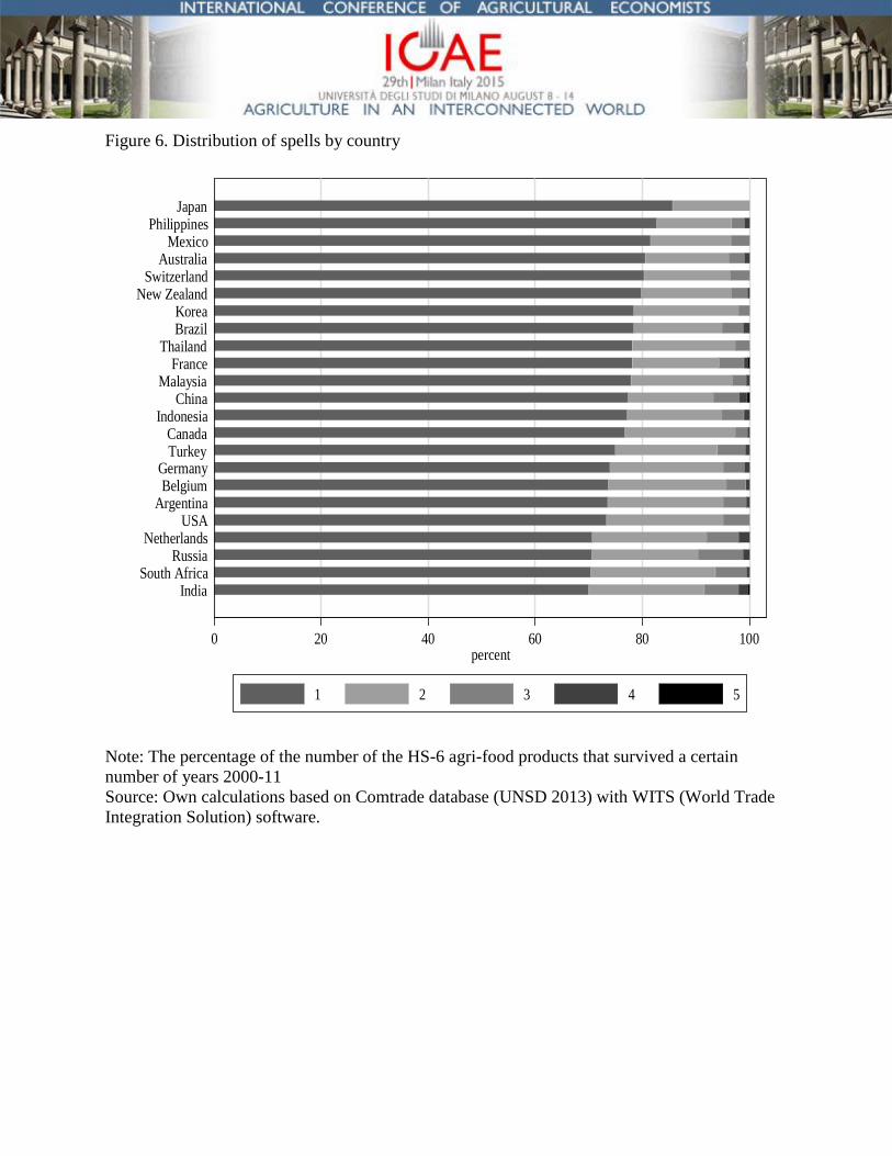
Figure 6. Distribution of spells by country
Note: The percentage of the number of the HS-6 agri-food products that survived a certain
number of years 2000-11
Source: Own calculations based on Comtrade database (UNSD 2013) with WITS (World Trade
Integration Solution) software.
0 20 40 60 80 100percent
IndiaSouth Africa
RussiaNetherlands
USAArgentina
BelgiumGermany
TurkeyCanada
IndonesiaChina
MalaysiaFrance
ThailandBrazilKorea
New ZealandSwitzerland
AustraliaMexico
PhilippinesJapan
1 2 3 4 5
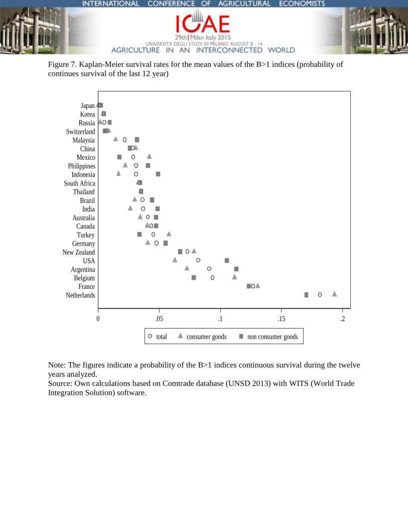
Figure 7. Kaplan-Meier survival rates for the mean values of the B>1 indices (probability of
continues survival of the last 12 year)
Note: The figures indicate a probability of the B>1 indices continuous survival during the twelve
years analyzed.
Source: Own calculations based on Comtrade database (UNSD 2013) with WITS (World Trade
Integration Solution) software.
0 .05 .1 .15 .2
Netherlands
FranceBelgium
Argentina
USANew Zealand
GermanyTurkey
CanadaAustralia
IndiaBrazil
ThailandSouth Africa
IndonesiaPhilippines
MexicoChina
MalaysiaSwitzerland
RussiaKorea
Japan
total consumer goods non consumer goods