1

Global Adaptive Dynamic Programming forContinuous-Time Nonlinear Systems

Yu Jiang, Member, IEEE, Zhong-Ping Jiang, Fellow, IEEE

Abstract—This paper presents a novel method of globaladaptive dynamic programming (ADP) for the adaptive optimalcontrol of nonlinear polynomial systems. The strategy consistsof relaxing the problem of solving the Hamilton-Jacobi-Bellman(HJB) equation to an optimization problem, which is solved via anew policy iteration method. The proposed method distinguishesfrom previously known nonlinear ADP methods in that the neuralnetwork approximation is avoided, giving rise to significantcomputational improvement. Instead of semiglobally or locallystabilizing, the resultant control policy is globally stabilizing fora general class of nonlinear polynomial systems. Furthermore, inthe absence of the a priori knowledge of the system dynamics,an online learning method is devised to implement the proposedpolicy iteration technique by generalizing the current ADPtheory. Finally, three numerical examples are provided to validatethe effectiveness of the proposed method.

Index Terms—Adaptive dynamic programming, nonlinear sys-tems, optimal control, global stabilization.

I. INTRODUCTION

Dynamic programming [4] offers a theoretical way to solveoptimal control problems. However, it suffers from the in-herent computational complexity, also known as the curse ofdimensionality. Therefore, the need for approximative methodshas been recognized as early as in the late 1950s [5]. Within allthese methods, adaptive/approximate dynamic programming(ADP) [6], [7], [38], [46], [58], [60] is a class of heuristictechniques that solves for the cost function by searchingfor a suitable approximation. In particular, adaptive dynamicprogramming [58], [59] employs the idea from reinforcementlearning [49] to achieve online approximation of the costfunction, without using the knowledge of the system dynam-ics. ADP has been extensively studied for Markov decisionprocesses (see, for example, [7] and [38]), as well as dynamicsystems (see the review papers [29] and [55]). Stability issuesin ADP-based control systems design are addressed in [2],[31], [54]. A robustification of ADP, known as Robust-ADP orRADP, is recently developed by taking into account dynamicuncertainties [24].

To achieve online approximation of the cost function andthe control policy, neural networks are widely used in theprevious ADP architecture. Although neural networks can be

This work has been supported in part by the National Science Foundationunder Grants ECCS-1101401 and ECCS-1230040. The work was done whenY. Jiang was a PhD student in the Control and Networks Lab at New YorkUniversity Polytechnic School of Engineering.

Y. Jiang is with The MathWorks, 3 Apple Hill Dr, Natick, MA 01760,E-mail: yu.jiang@mathworks.com

Z. P. Jiang is with the Department of Electrical and Computer Engineering,Polytechnic School of Engineering, New York University, Five MetrotechCenter, Brooklyn, NY 11201 USA. zjiang@nyu.edu

used as universal approximators [18], [36], there are at leasttwo major limitations for ADP-based online implementations.First, in order to approximate unknown functions with highaccuracy, a large number of basis functions comprising theneural network are usually required. Hence, it may incur ahuge computational burden for the learning system. Besides,it is not trivial to specify the type of basis functions, whenthe target function to be approximated is unknown. Second,neural network approximations generally are effective only onsome compact sets, but not in the entire state space. Therefore,the resultant control policy may not provide global asymptoticstability for the closed-loop system. In addition, the compactset, on which the uncertain functions of interest are to beapproximated, has to be carefully quantified before one appliesthe online learning method, such that stability can be assuredduring the learning process [22].

The main purpose of this paper is to develop a novelADP methodology to achieve global and adaptive suboptimalstabilization of uncertain continuous-time nonlinear polyno-mial systems via online learning. As the first contribution ofthis paper, an optimization problem, of which the solutionscan be easily parameterized, is proposed to relax the prob-lem of solving the Hamilton-Jacobi-Bellman (HJB) equation.This approach is inspired from the relaxation method usedin approximate dynamic programming for Markov decisionprocesses (MDPs) with finite state space [13], and moregeneralized discrete-time systems [32], [56], [57], [43], [44],[48]. However, methods developed in these papers cannot betrivially extended to the continuous-time setting, or achieveglobal asymptotic stability of general nonlinear systems. Theidea of relaxation was also used in nonlinear H∞ control,where Hamilton-Jacobi inequalities are used for nonadaptivesystems [16], [51], [42].

The second contribution of the paper is to propose a relaxedpolicy iteration method. Each iteration step is formulated as asum of squares (SOS) program [37], [10], which is equivalentto a semidefinite program (SDP). It is worth pointing out that,different from the inverse optimal control design [27], theproposed method finds directly a suboptimal solution to theoriginal optimal control problem.

The third contribution is an online learning method thatimplements the proposed iterative schemes using only the real-time online measurements, when the perfect system knowledgeis not available. This method can be regarded as a nonlinearvariant of our recent work for continuous-time linear systemswith completely unknown system dynamics [23]. This methoddistinguishes from previously known nonlinear ADP methodsin that the neural network approximation is avoided for com-

arX

iv:1

401.

0020

v4 [

mat

h.D

S] 1

0 Ja

n 20

17

2

putational benefits and that the resultant suboptimal controlpolicy achieves global asymptotic stabilization, instead of onlysemi-global or local stabilization.

The remainder of this paper is organized as follows. Section2 formulates the problem and introduces some basic resultsregarding nonlinear optimal control. Section 3 relaxes theproblem of solving an HJB equation to an optimization prob-lem. Section 4 develops a relaxed policy iteration techniquefor polynomial systems using sum of squares (SOS) programs[10]. Section 5 develops an online learning method for apply-ing the proposed policy iteration, when the system dynamicsare not known exactly. Section 6 examines three numericalexamples to validate the efficiency and effectiveness of theproposed method. Section 7 gives concluding remarks.

Notations: Throughout this paper, we use C1 to denote theset of all continuously differentiable functions. P denotes theset of all functions in C1 that are also positive definite andproper. R+ indicates the set of all non-negative real numbers.For any vector u ∈ Rm and any symmetric matrix R ∈ Rm×m,we define |u|2R as uTRu. A feedback control policy u is calledglobally stabilizing, if under this control policy, the closed-loop system is globally asymptotically stable at the origin[26]. Given a vector of polynomials f(x), deg(f) denotes thehighest polynomial degree of all the entries in f(x). For anypositive integers d1, d2 satisfying d2 ≥ d1, ~md1,d2(x) is thevector of all (n+d2

d2)− (n+d1−1

d1−1 ) distinct monic monomials inx ∈ Rn with degree at least d1 and at most d2, and arrangedin lexicographic order [12]. Also, R[x]d1,d2 denotes the set ofall polynomials in x ∈ Rn with degree no less than d1 andno greater than d2. ∇V refers to the gradient of a functionV : Rn → R.

II. PROBLEM FORMULATION AND PRELIMINARIES

A. Problem formulation

Consider the nonlinear system

x = f(x) + g(x)u (1)

where x ∈ Rn is the system state, u ∈ Rm is the control input,f : Rn → Rn and g : Rn → Rn×m are polynomial mappingswith f(0) = 0.

In conventional optimal control theory [30], the commonobjective is to find a control policy u that minimizes certainperformance index. In this paper, it is specified as follows.

J(x0, u) =

∫ ∞0

r(x(t), u(t))dt, x(0) = x0 (2)

where r(x, u) = q(x)+uTR(x)u, with q(x) a positive definitepolynomial function, and R(x) is a symmetric positive definitematrix of polynomials. Notice that, the purpose of specifyingr(x, u) in this form is to guarantee that an optimal controlpolicy can be explicitly determined, if it exists.

Assumption 2.1: Consider system (1). There exist a func-tion V0 ∈ P and a feedback control policy u1, such that

L(V0(x), u1(x)) ≥ 0, ∀x ∈ Rn (3)

where, for any V ∈ C1 and u ∈ Rm,

L(V, u) = −∇V T (x)(f(x) + g(x)u)− r(x, u). (4)

Under Assumption 2.1, the closed-loop system composedof (1) and u = u1(x) is globally asymptotically stable at theorigin, with a well-defined Lyapunov function V0. With thisproperty, u1 is also known as an admissible control policy[3], implying that the cost J(x0, u1) is finite, ∀x0 ∈ Rn.Indeed, integrating both sides of (3) along the trajectories ofthe closed-loop system composed of (1) and u = u1(x) onthe interval [0,+∞), it is easy to show that

J(x0, u1) ≤ V0(x0), ∀x0 ∈ Rn. (5)

B. Optimality and stability

Here, we recall a basic result connecting optimality andglobal asymptotic stability in nonlinear systems [45].

To begin with, let us give the following assumption.Assumption 2.2: There exists V o ∈ P , such that the

Hamilton-Jacobi-Bellman (HJB) equation holds

H(V o) = 0 (6)

where

H(V ) = ∇V T (x)f(x) + q(x)

−1

4∇V T (x)g(x)R−1(x)gT (x)∇V (x).

Under Assumption 2.2, it is easy to see that V o is awell-defined Lyapunov function for the closed-loop systemcomprised of (1) and

uo(x) = −1

2R−1(x)gT (x)∇V o(x). (7)

Hence, this closed-loop system is globally asymptoticallystable at x = 0 [26]. Then, according to [45, Theorem 3.19],uo is the optimal control policy, and the value function V o(x0)gives the optimal cost at the initial condition x(0) = x0, i.e.,

V o(x0) = minuJ(x0, u) = J(x0, u

o), ∀x0 ∈ Rn. (8)

It can also be shown that V o is the unique solution to theHJB equation (6) with V o ∈ P . Indeed, let V ∈ P be anothersolution to (6). Then, by Theorem 3.19 in [45], along thesolutions of the closed-loop system composed of (1) and u =u = − 1

2R−1gT∇V , it follows that

V (x0) = V o(x0)−∫ ∞

0

|uo − u|2Rdt, ∀x0 ∈ Rn. (9)

Finally, by comparing (8) and (9), we conclude that

V o = V .

C. Conventional policy iteration

The above-mentioned result implies that, if there existsa class-P function which solves the HJB equation (6), anoptimal control policy can be obtained. However, the nonlinearHJB equation (6) is very difficult to be solved analyticallyin general. As a result, numerical methods are developed toapproximate the solution. In particular, the following policyiteration method is widely used [41].

3

1) Policy evaluation: For i = 1, 2, · · · , solve for the costfunction Vi(x) ∈ C1, with Vi(0) = 0, from the followingpartial differential equation.

L(Vi(x), ui(x)) = 0. (10)

2) Policy improvement: Update the control policy by

ui+1(x) = −1

2R−1(x)gT (x)∇Vi(x). (11)

The convergence property of the conventional policy itera-tion algorithm is given in the following theorem, which is anextension of [41, Theorem 4]. For the readers’ convenience,its proof is given in Appendix B.

Theorem 2.3: Suppose Assumptions 2.1 and 2.2 hold, andthe solution Vi(x) ∈ C1 satisfying (10) exists, for i = 1, 2, · · · .Let Vi(x) and ui+1(x) be the functions generated from (10)and (11). Then, the following properties hold, ∀i = 0, 1, · · · .

1) V o(x) ≤ Vi+1(x) ≤ Vi(x), ∀x ∈ Rn;2) ui+1 is globally stabilizing;3) suppose there exist V ∗ ∈ C1 and u∗, such that ∀x0 ∈

Rn, we have limi→∞

Vi(x0) = V ∗(x0) and limi→∞

ui(x0) =

u∗(x0). Then, V ∗ = V o and u∗ = uo.Notice that finding the analytical solution to (10) is still

non-trivial. Hence, in practice, the solution is approximatedusing, for example, neural networks or Galerkin’s method[3]. Also, ADP-based online approximation method can beapplied to compute numerically the cost functions via onlinedata [53], [22], when the precise knowledge of f or g is notavailable. However, although approximation methods can giveacceptable results on some compact set in the state space, theycannot be used to achieve global stabilization. In addition, inorder to reduce the approximation error, huge computationalcomplexity is almost inevitable.

III. SUBOPTIMAL CONTROL WITH RELAXED HJBEQUATION

In this section, we consider an auxiliary optimization prob-lem, which allows us to obtain a suboptimal solution to theminimization problem (2) subject to (1). For simplicity, wewill omit the arguments of functions whenever there is noconfusion in the context.

Problem 3.1 (Relaxed optimal control problem):

minV

∫ΩV (x)dx (12)

s.t. H(V ) ≤ 0 (13)V ∈ P (14)

where Ω ⊂ Rn is an arbitrary compact set containing theorigin as an interior point. As a subset of the state space, Ωdescribes the area in which the system performance is expectedto be improved the most.

Remark 3.2: Notice that Problem 3.1 is called a relaxedproblem of (6). Indeed, if we restrict this problem by replacingthe inequality constraint (13) with the equality constraint (6),there will be only one feasible solution left and the objectivefunction can thus be neglected. As a result, Problem 3.1reduces to the problem of solving (6).

Some useful facts about Problem 3.1 are given as follows.Theorem 3.3: Under Assumptions 2.1 and 2.2, the follow-

ing hold.1) Problem 3.1 has a nonempty feasible set.2) Let V be a feasible solution to Problem 3.1. Then, the

control policy

u(x) = −1

2R−1gT∇V (15)

is globally stabilizing.3) For any x0 ∈ Rn, an upper bound of the cost of the

closed-loop system comprised of (1) and (15) is givenby V (x0), i.e.,

J(x0, u) ≤ V (x0). (16)

4) Along the trajectories of the closed-loop system (1) and(7), the following inequalities hold for any x0 ∈ Rn:

V (x0) +

∫ ∞0

H(V (x(t)))dt ≤ V o(x0) ≤ V (x0). (17)

5) V o as defined in (8) is a global optimal solution toProblem 3.1.

Proof:

1) Define u0 = −1

2R−1gT∇V0. Then,

H(V0) = ∇V T0 (f + gu0) + r(x, u0)

= ∇V T0 (f + gu1) + r(x, u1)

+∇V T0 g(u0 − u1) + |u0|2R − |u1|2R= ∇V T0 (f + gu1) + r(x, u1)

−2|u0|2R − 2uT0 Ru1 + |u0|2R − |u1|2R= ∇V T0 (f + gu1) + r(x, u1)− |u0 − u1|2R≤ 0

Hence, V0 is a feasible solution to Problem 3.1.2) To show global asymptotic stability, we only need to

prove that V is a well-defined Lyapunov function for theclosed-loop system composed of (1) and (15). Indeed, alongthe solutions of the closed-loop system, it follows that

V = ∇V T (f + gu)

= H(V )− r(x, u)

≤ −q(x)

Therefore, the system is globally asymptotically stable at theorigin [26].

3) Along the solutions of the closed-loop system comprisedof (1) and (15), we have

V (x0) = −∫ T

0

∇V T (f + gu)dt+ V (x(T ))

=

∫ T

0

[r(x, u)−H(V )] dt+ V (x(T ))

≥∫ T

0

r(x, u)dt+ V (x(T )) (18)

By 2), limT→+∞

V (x(T )) = 0. Therefore, letting T → +∞,

by (18) and (2), we have

V (x0) ≥ J(x0, u). (19)

4

4) By 3), we have

V (x0) ≥ J(x0, u) ≥ minuJ(x0, u) = V o(x0). (20)

Hence, the second inequality in (17) is proved.On the other hand,

H(V ) = H(V )−H(V o)

= (∇V −∇V o)T (f + gu) + r(x, u)

−(∇V o)T g(uo − u)− r(x, uo)

= (∇V −∇V o)T (f + guo)− |u− uo|2R≤ (∇V −∇V o)T (f + guo)

Integrating the above equation along the solutions of theclosed-loop system (1) and (7) on the interval [0,+∞), wehave

V (x0)− V o(x0) ≤ −∫ ∞

0

H(V (x))dt. (21)

5) By 3), for any feasible solution V to Problem 3.1, wehave V o(x) ≤ V (x). Hence,∫

Ω

V o(x)dx ≤∫

Ω

V (x)dx (22)

which implies that V o is a global optimal solution.The proof is therefore complete.Remark 3.4: A feasible solution V to Problem 3.1 may

not necessarily be the true cost function associated with thecontrol policy u defined in (15). However, by Theorem 3.3,we see V can be viewed as an upper bound or an overestimateof the actual cost, inspired by the concept of underestimator in[56]. Further, V serves as a Lyapunov function for the closed-loop system and can be more easily parameterized than theactual cost function. For simplicity, V is still called the costfunction, in the remainder of the paper.

IV. SOS-BASED POLICY ITERATION FOR POLYNOMIALSYSTEMS

The inequality constraint (13) contained in Problem 3.1provides us the freedom of specifying desired analytical formsof the cost function. However, solving (13) is non-trivial ingeneral, even for polynomial systems (see, for example, [11],[14], [34], [47], [61]). Indeed, for any polynomial with degreeno less than four, deciding its non-negativity is an NP-hardproblem [37]. Thanks to the developments in sum of squares(SOS) programs [10], [37], the computational burden can besignificantly reduced, if inequality constraints can be restrictedto SOS constraints. The purpose of this section is to developa novel policy iteration method for polynomial systems usingSOS-based methods [10], [37].

A. Polynomial parametrization

Let us first assume R(x) is a constant, real symmetricmatrix. Notice that L(Vi, ui) is a polynomial in x, if ui is apolynomial control policy and Vi is a polynomial cost function.Then, the following implication holds

L(Vi, ui) is SOS⇒ L(Vi, ui) ≥ 0. (23)

In addition, for computational simplicity, we would like tofind some positive integer r, such that Vi ∈ R[x]2,2r. Then,the new control policy ui+1 obtained from (27) is a vector ofpolynomials.

Based on the above discussion, the following Assumptionis given to replace Assumption 2.1.

Assumption 4.1: There exist smooth mappings V0 : Rn →R and u1 : Rn → Rm, such that V0 ∈ R[x]2,2r ∩ P andL(V0, u1) is SOS.

B. SOS-programming-based policy iteration

Now, we are ready to propose a relaxed policy iterationscheme. Similar as in other policy-iteration-based iterativeschemes, an initial globally stabilizing (and admissible) controlpolicy has been assumed in Assumption 4.1.

1) Policy evaluation: For i = 1, 2, · · · , solve for an optimalsolution pi to the following optimization program:

minp

∫Ω

V (x)dx (24)

s.t. L(V, ui) is SOS (25)Vi−1 − V is SOS (26)

where V = pT ~m2,2r(x). Then, denote Vi =pTi ~m2,2r(x).

2) Policy improvement: Update the control policy by

ui+1 = −1

2R−1gT∇Vi. (27)

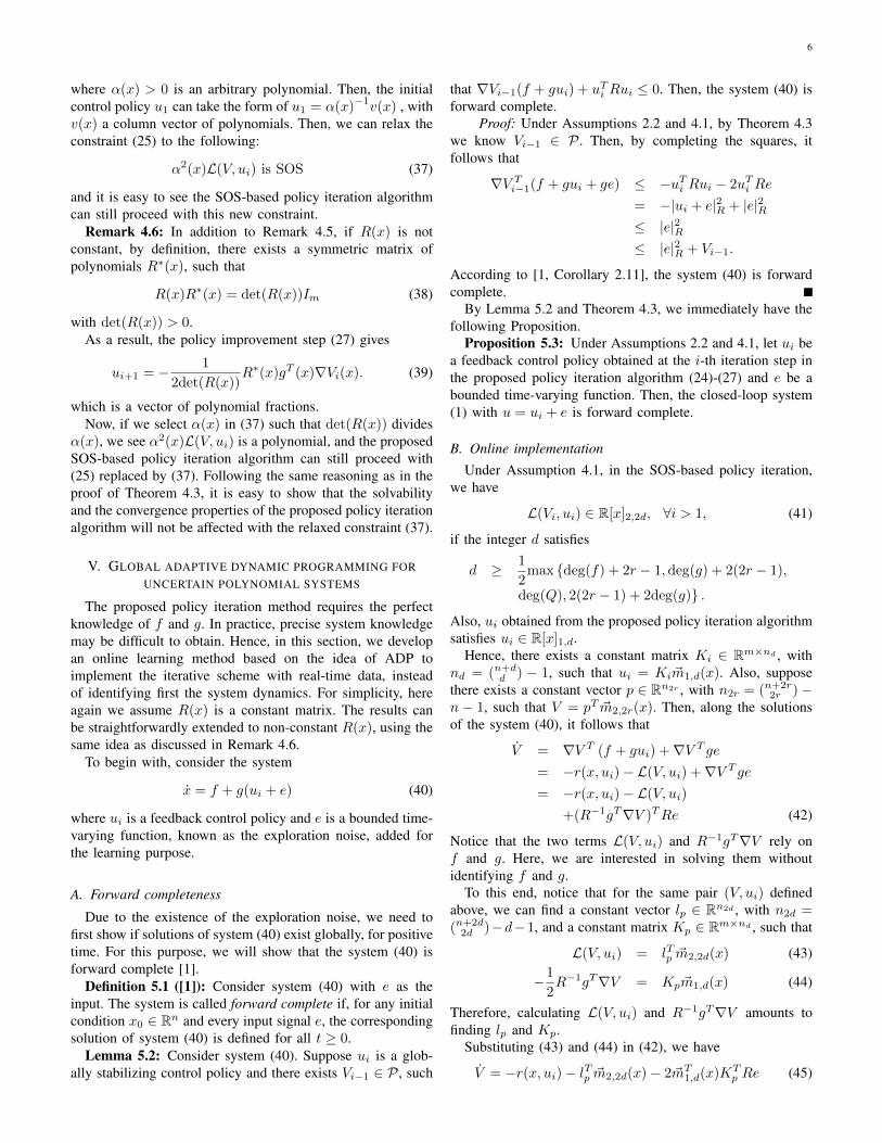
Then, go to Step 1) with i replaced by i+ 1.A flowchart of the practical implementation is given in

Figure 1, where ε > 0 is a predefined threshold to balancethe exploration/exploitation trade-off. In practice, a larger εmay lead to shorter exploration time and therefore will allowthe system to implement the control policy and terminate theexploration noise sooner. On the other hand, using a smaller εallows the learning system to better improve the control policybut needs longer learning time.

StartInitialization: Find (V0, u1) thatsatisfy Assumption 4.1. i← 1.

Policy Evaluation: Solve Vi =pTi ~mr,2r(x) from (24)-(26).

Policy Improvement: Update thecontrol policy to ui+1 by (27).

|pi − pi−1| ≤ ε

Use u = ui as thecontrol input. Stop

i← i+ 1

Yes

No

Fig. 1. Flowchart of the SOS-programming-based policy iteration.

5

Remark 4.2: The optimization problem (24)-(26) is a well-defined SOS program [10]. Indeed, the objective function (24)is linear in p, since for any V = pT ~m2,2r(x), we have∫

ΩV (x)dx = cT p, with c =

∫Ω~m2,2r(x)dx.

Theorem 4.3: Under Assumptions 2.2 and 4.1, the follow-ing are true, for i = 1, 2, · · · .

1) The SOS program (24)-(26) has a nonempty feasible set.2) The closed-loop system comprised of (1) and u = ui is

globally asymptotically stable at the origin.3) Vi ∈ P . In particular, the following inequalities hold:

V o(x0) ≤ Vi(x0) ≤ Vi−1(x0), ∀x0 ∈ Rn. (28)

4) There exists V ∗(x) satisfying V ∗(x) ∈ R[x]2,2r ∩ P ,such that, for any x0 ∈ Rn, lim

i→∞Vi(x0) = V ∗(x0).

5) Along the solutions of the system comprised of (1) and(7), the following inequalities hold:

0 ≤ V ∗(x0)− V o(x0) ≤ −∫ ∞

0

H(V ∗(x(t)))dt. (29)

Proof: 1) We prove by mathematical induction.i) Suppose i = 1, under Assumption 4.1, we know

L(V0, u1) is SOS. Hence, V = V0 is a feasible solution tothe problem (24)-(26).

ii) Let V = Vj−1 be an optimal solution to the problem(24)-(26) with i = j − 1 > 1. We show that V = Vj−1 is afeasible solution to the same problem with i = j.

Indeed, by definition,

uj = −1

2R−1gT∇Vj−1,

and

L(Vj−1, uj) = −∇V Tj−1(f + guj)− r(x, uj)= L(Vj−1, uj−1)−∇V Tj−1g(uj − uj−1)

+uTj−1Ruj−1 − uTj Ruj= L(Vj−1, uj−1) + |uj − uj−1|2R.

Under the induction assumption, we know Vj−1 ∈ R[x]2,2rand L(Vj−1, uj−1) is SOS. Hence, L(Vj−1, uj) is SOS. As aresult, Vj−1 is a feasible solution to the SOS program (24)-(26) with i = j.

2) Again, we prove by induction.i) Suppose i = 1, under Assumption 4.1, u1 is globally

stabilizing. Also, we can show that V1 ∈ P . Indeed, for eachx0 ∈ Rn with x0 6= 0, we have

V1(x0) ≥∫ ∞

0

r(x, u1)dt > 0. (30)

By (30) and the constraint (26), under Assumption 2.2 itfollows that

V o ≤ V1 ≤ V0. (31)

Since both V o and V0 are assumed to belong to P , weconclude that V1 ∈ P .

ii) Suppose ui−1 is globally stabilizing, and Vi−1 ∈ P fori > 1. Let us show that ui is globally stabilizing, and Vi ∈ P .

Indeed, along the solutions of the closed-loop system com-posed of (1) and u = ui, it follows that

Vi−1 = ∇V Ti−1(f + gui)

= −L(Vi−1, ui)− r(x, ui)≤ −q(x).

Therefore, ui is globally stabilizing, since Vi−1 is a well-defined Lyapunov function for the system. In addition, wehave

Vi(x0) ≥∫ ∞

0

r(x, ui)dt > 0, ∀x0 6= 0. (32)

Similarly as in (31), we can show

V o(x0) ≤ Vi(x0) ≤ Vi−1(x0), ∀x0 ∈ Rn, (33)

and conclude that Vi ∈ P .3) The two inequalities have been proved in (33).4) By 3), for each x ∈ Rn, the sequence Vi(x)∞i=0 is

monotonically decreasing with 0 as its lower bound. There-fore, the limit exists, i.e., there exists V ∗(x), such thatlimi→∞

Vi(x) = V ∗(x). Let pi∞i=1 be the sequence such that

Vi = pTi ~m2,2r(x). Then, we know limi→∞

pi = p∗ ∈ Rn2r ,

and therefore V ∗ = p∗T ~m2,2r(x). Also, it is easy to showV o ≤ V ∗ ≤ V0. Hence, V ∗ ∈ R[x]2,2r ∩ P .

5) Let

u∗ = −1

2R−1gT∇V ∗, (34)

Then, by 4) we know

H(V ∗) = −L(V ∗, u∗) ≤ 0, (35)

which implies that V ∗ is a feasible solution to Problem 3.1.The inequalities in 5) can thus be obtained by the fourthproperty in Theorem 3.3.

The proof is thus complete.Remark 4.4: Notice that Assumption 4.1 holds for any

controllable linear systems. For general nonlinear systems,such a pair (V0, u1) satisfying Assumption 4.1 may not alwaysexist, and in this paper we focus on polynomial systems thatsatisfy Assumption 4.1. For this class of systems, we assumethat both V0 and u1 have to be determined before executingthe proposed algorithm. The search of (V0, u1) is not trivial,because it amounts to solving some bilinear matrix inequalities(BMI) [40]. However, this problem has been actively studiedin recent years, and several applicable approaches have beendeveloped. For example, a Lyapunov based approach utilizingstate-dependent linear matrix inequalities has been studied in[40]. This method has been generalized to uncertain nonlinearpolynomial systems in [61] and [20]. In [19] and [28], theauthors proposed a solution for a stochastic HJB. It is shownthat this method gives a control Lyapunov function for thedeterministic system.

Remark 4.5: Notice that the control policies consideredin the proposed algorithm can be extended to polynomialfractions. Indeed, instead of requiring L(V0, u1) to be SOSin Assumption 4.1, let us assume

α2(x)L(V0, u1) is SOS (36)

6

where α(x) > 0 is an arbitrary polynomial. Then, the initialcontrol policy u1 can take the form of u1 = α(x)

−1v(x) , with

v(x) a column vector of polynomials. Then, we can relax theconstraint (25) to the following:

α2(x)L(V, ui) is SOS (37)

and it is easy to see the SOS-based policy iteration algorithmcan still proceed with this new constraint.

Remark 4.6: In addition to Remark 4.5, if R(x) is notconstant, by definition, there exists a symmetric matrix ofpolynomials R∗(x), such that

R(x)R∗(x) = det(R(x))Im (38)

with det(R(x)) > 0.As a result, the policy improvement step (27) gives

ui+1 = − 1

2det(R(x))R∗(x)gT (x)∇Vi(x). (39)

which is a vector of polynomial fractions.Now, if we select α(x) in (37) such that det(R(x)) divides

α(x), we see α2(x)L(V, ui) is a polynomial, and the proposedSOS-based policy iteration algorithm can still proceed with(25) replaced by (37). Following the same reasoning as in theproof of Theorem 4.3, it is easy to show that the solvabilityand the convergence properties of the proposed policy iterationalgorithm will not be affected with the relaxed constraint (37).

V. GLOBAL ADAPTIVE DYNAMIC PROGRAMMING FORUNCERTAIN POLYNOMIAL SYSTEMS

The proposed policy iteration method requires the perfectknowledge of f and g. In practice, precise system knowledgemay be difficult to obtain. Hence, in this section, we developan online learning method based on the idea of ADP toimplement the iterative scheme with real-time data, insteadof identifying first the system dynamics. For simplicity, hereagain we assume R(x) is a constant matrix. The results canbe straightforwardly extended to non-constant R(x), using thesame idea as discussed in Remark 4.6.

To begin with, consider the system

x = f + g(ui + e) (40)

where ui is a feedback control policy and e is a bounded time-varying function, known as the exploration noise, added forthe learning purpose.

A. Forward completeness

Due to the existence of the exploration noise, we need tofirst show if solutions of system (40) exist globally, for positivetime. For this purpose, we will show that the system (40) isforward complete [1].

Definition 5.1 ([1]): Consider system (40) with e as theinput. The system is called forward complete if, for any initialcondition x0 ∈ Rn and every input signal e, the correspondingsolution of system (40) is defined for all t ≥ 0.

Lemma 5.2: Consider system (40). Suppose ui is a glob-ally stabilizing control policy and there exists Vi−1 ∈ P , such

that ∇Vi−1(f + gui) + uTi Rui ≤ 0. Then, the system (40) isforward complete.

Proof: Under Assumptions 2.2 and 4.1, by Theorem 4.3we know Vi−1 ∈ P . Then, by completing the squares, itfollows that

∇V Ti−1(f + gui + ge) ≤ −uTi Rui − 2uTi Re

= −|ui + e|2R + |e|2R≤ |e|2R≤ |e|2R + Vi−1.

According to [1, Corollary 2.11], the system (40) is forwardcomplete.

By Lemma 5.2 and Theorem 4.3, we immediately have thefollowing Proposition.

Proposition 5.3: Under Assumptions 2.2 and 4.1, let ui bea feedback control policy obtained at the i-th iteration step inthe proposed policy iteration algorithm (24)-(27) and e be abounded time-varying function. Then, the closed-loop system(1) with u = ui + e is forward complete.

B. Online implementation

Under Assumption 4.1, in the SOS-based policy iteration,we have

L(Vi, ui) ∈ R[x]2,2d, ∀i > 1, (41)

if the integer d satisfies

d ≥ 1

2max deg(f) + 2r − 1,deg(g) + 2(2r − 1),

deg(Q), 2(2r − 1) + 2deg(g) .

Also, ui obtained from the proposed policy iteration algorithmsatisfies ui ∈ R[x]1,d.

Hence, there exists a constant matrix Ki ∈ Rm×nd , withnd = (n+d

d ) − 1, such that ui = Ki ~m1,d(x). Also, supposethere exists a constant vector p ∈ Rn2r , with n2r = (n+2r

2r )−n − 1, such that V = pT ~m2,2r(x). Then, along the solutionsof the system (40), it follows that

V = ∇V T (f + gui) +∇V T ge= −r(x, ui)− L(V, ui) +∇V T ge= −r(x, ui)− L(V, ui)

+(R−1gT∇V )TRe (42)

Notice that the two terms L(V, ui) and R−1gT∇V rely onf and g. Here, we are interested in solving them withoutidentifying f and g.

To this end, notice that for the same pair (V, ui) definedabove, we can find a constant vector lp ∈ Rn2d , with n2d =(n+2d

2d )−d−1, and a constant matrix Kp ∈ Rm×nd , such that

L(V, ui) = lTp ~m2,2d(x) (43)

−1

2R−1gT∇V = Kp ~m1,d(x) (44)

Therefore, calculating L(V, ui) and R−1gT∇V amounts tofinding lp and Kp.

Substituting (43) and (44) in (42), we have

V = −r(x, ui)− lTp ~m2,2d(x)− 2~mT1,d(x)KT

p Re (45)

7

Now, integrating the terms in (45) over the interval [t, t+δt],we have

pT [~m2,2r(x(t))− ~m2,2r(x(t+ δt))]

=

∫ t+δt

t

(r(x, ui) + lTp ~m2,2d(x)

+2~mT1,d(x)KT

p Re)dt (46)

Eq. (46) implies that, lp and Kp can be directly calculatedby using real-time online data, without knowing the preciseknowledge of f and g.

To see how it works, let us define the following matrices:σe ∈ Rn2d+mnd , Φi ∈ Rqi×(n2d+mnd), Ξi ∈ Rqi , Θi ∈Rqi×n2r , such that

σe = −[~mT

2,2d 2~mT1,d ⊗ eTR

]T,

Φi =[ ∫ t1,i

t0,iσedt

∫ t2,it1,i

σedt · · ·∫ tqi,itqi−1,i

σedt]T,

Ξi =[ ∫ t1,i

t0,ir(x, ui)dt

∫ t2,it1,i

r(x, ui)dt · · ·∫ tqi,itqi−1,i

r(x, ui)dt]T,

Θi =[~m2,2r|

t1,it0,i ~m2,2r|

t2,it1,i · · · ~m2,2r|

tqi,itqi−1,i

]T.

Then, (46) implies

Φi

[lp

vec(Kp)

]= Ξi + Θip. (47)

Notice that any pair of (lp,Kp) satisfying (47) will satisfythe constraint between lp and Kp as implicitly indicated in(45) and (46).

Assumption 5.4: For each i = 1, 2, · · · , there exists aninteger qi0, such that the following rank condition holds,

rank(Φi) = n2d +mnd, (48)

if qi ≥ qi0.Remark 5.5: This rank condition (48) is in the spirit of

persistency of excitation (PE) in adaptive control (e.g. [21],[50]) and is a necessary condition for parameter convergence.

Given p ∈ Rn2r and Ki ∈ Rm×nd , suppose Assumption 5.4is satisfied and qi ≥ qi0 for all i = 1, 2, · · · . Then, it is easy tosee that the values of lp and Kp can be uniquely determinedfrom (46). Indeed,[

lpvec(Kp)

]=(ΦTi Φi

)−1ΦTi (Ξi + Θip) (49)

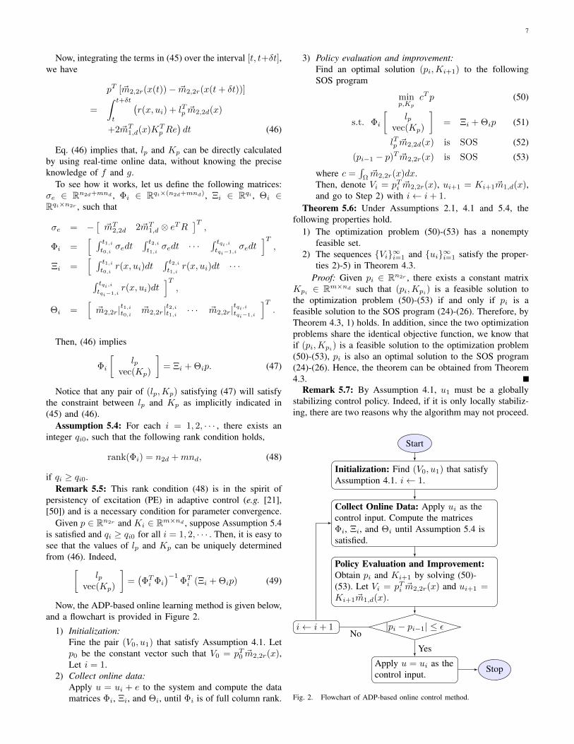
Now, the ADP-based online learning method is given below,and a flowchart is provided in Figure 2.

1) Initialization:Fine the pair (V0, u1) that satisfy Assumption 4.1. Letp0 be the constant vector such that V0 = pT0 ~m2,2r(x),Let i = 1.

2) Collect online data:Apply u = ui + e to the system and compute the datamatrices Φi, Ξi, and Θi, until Φi is of full column rank.

3) Policy evaluation and improvement:Find an optimal solution (pi,Ki+1) to the followingSOS program

minp,Kp

cT p (50)

s.t. Φi

[lp

vec(Kp)

]= Ξi + Θip (51)

lTp ~m2,2d(x) is SOS (52)

(pi−1 − p)T ~m2,2r(x) is SOS (53)

where c =∫

Ω~m2,2r(x)dx.

Then, denote Vi = pTi ~m2,2r(x), ui+1 = Ki+1 ~m1,d(x),and go to Step 2) with i← i+ 1.

Theorem 5.6: Under Assumptions 2.1, 4.1 and 5.4, thefollowing properties hold.

1) The optimization problem (50)-(53) has a nonemptyfeasible set.

2) The sequences Vi∞i=1 and ui∞i=1 satisfy the proper-ties 2)-5) in Theorem 4.3.

Proof: Given pi ∈ Rn2r , there exists a constant matrixKpi ∈ Rm×nd such that (pi,Kpi) is a feasible solution tothe optimization problem (50)-(53) if and only if pi is afeasible solution to the SOS program (24)-(26). Therefore, byTheorem 4.3, 1) holds. In addition, since the two optimizationproblems share the identical objective function, we know thatif (pi,Kpi) is a feasible solution to the optimization problem(50)-(53), pi is also an optimal solution to the SOS program(24)-(26). Hence, the theorem can be obtained from Theorem4.3.

Remark 5.7: By Assumption 4.1, u1 must be a globallystabilizing control policy. Indeed, if it is only locally stabiliz-ing, there are two reasons why the algorithm may not proceed.

Start

Initialization: Find (V0, u1) that satisfyAssumption 4.1. i← 1.

Collect Online Data: Apply ui as thecontrol input. Compute the matricesΦi, Ξi, and Θi until Assumption 5.4 issatisfied.

Policy Evaluation and Improvement:Obtain pi and Ki+1 by solving (50)-(53). Let Vi = pTi ~m2,2r(x) and ui+1 =Ki+1 ~m1,d(x).

|pi − pi−1| ≤ ε

Apply u = ui as thecontrol input. Stop

i← i+ 1

Yes

No

Fig. 2. Flowchart of ADP-based online control method.

8

First, with a locally stabilizing control law, there is no wayto guarantee the forward completeness of solutions, or avoidfinite escape, during the learning phase. Second, the regionof attraction associated with the new control policy is notguaranteed to be global. Such a counterexample is x = θx3+uwith unknown positive θ, for which the choice of a locallystabilizing controller u1 = −x does not lead to a globallystabilizing suboptimal controller.

VI. APPLICATIONS

A. A scalar nonlinear polynomial system

Consider the following polynomial system

x = ax2 + bu (54)

where x ∈ R is the system state, u ∈ R is the controlinput, a and b, satisfying a ∈ [0, 0.05] and b ∈ [0.5, 1], areuncertain constants. The cost to be minimized is defined asJ(x0, u) =

∫∞0

(0.01x2+0.01x4+u2)dt. An initial stabilizingcontrol policy can be selected as u1 = −0.1x− 0.1x3, whichglobally asymptotically stabilizes system (54), for any a andb satisfying the given range. Further, it is easy to see thatV0 = 10(x2 + x4) and u1 satisfy Assumption 4.1 with r = 2.In addition, we set d = 3.

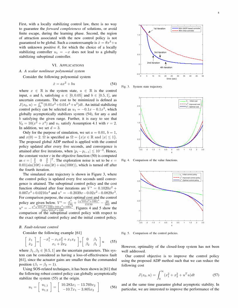
Only for the purpose of simulation, we set a = 0.01, b = 1,and x(0) = 2. Ω is specified as Ω = x|x ∈ R and |x| ≤ 1.The proposed global ADP method is applied with the controlpolicy updated after every five seconds, and convergence isattained after five iterations, when |pi−pi−1| ≤ 10−3. Hence,the constant vector c in the objective function (50) is computedas c = [ 2

3 0 25 ]T . The exploration noise is set to be e =

0.01(sin(10t) + sin(3t) + sin(100t)), which is turned off afterthe fourth iteration.

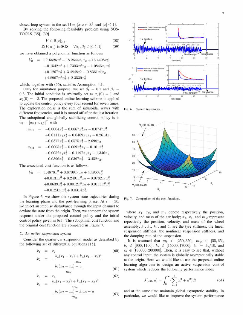
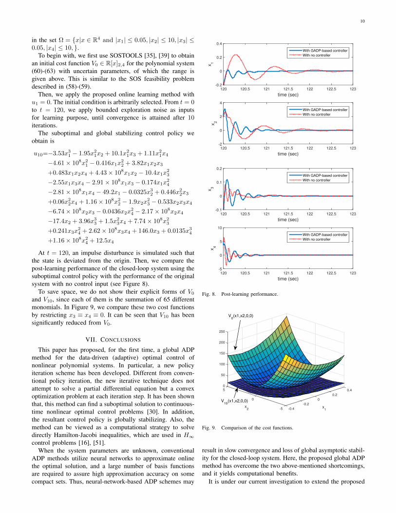
The simulated state trajectory is shown in Figure 3, wherethe control policy is updated every five seconds until conver-gence is attained. The suboptimal control policy and the costfunction obtained after four iterations are V ∗ = 0.1020x2 +0.007x3+0.0210x4 and u∗ = −0.2039x−0.02x2−0.0829x3.For comparison purpose, the exact optimal cost and the controlpolicy are given below. V o = x3

150 + (√

101x2+100)3

15150 − 20303 and

uo = −x2√

101x2+100+101x4+100x2

100√

101x2+100. Figures 4 and 5 show the

comparison of the suboptimal control policy with respect tothe exact optimal control policy and the initial control policy.

B. Fault-tolerant control

Consider the following example [61][x1

x2

]=

[−x3

1 − x1x22 + x1x2

x1 + 2x2

]+

[0 β1

β2 β1

]u (55)

where β1, β2 ∈ [0.5, 1] are the uncertain parameters. This sys-tem can be considered as having a loss-of-effectiveness fault[61], since the actuator gains are smaller than the commandedposition (β1 = β2 = 1).

Using SOS-related techniques, it has been shown in [61] thatthe following robust control policy can globally asymptoticallystabilize the system (55) at the origin.

u1 =

[u1,1

u1,2

]=

[10.283x1 − 13.769x2

−10.7x1 − 3.805x2

](56)

time (sec)

0 5 10 15 20 25 30 35 40 45 50-0.5

0

0.5

1

1.5

2

With GADP-based controller

With initial controller1st iteration

4th iteration

3rd iteration

2nd iteration

Fig. 3. System state trajectory.

x

-2.5 -2 -1.5 -1 -0.5 0 0.5 1 1.5 2 2.50

0.5

1

1.5

2

2.5

3

V1 : Initial cost

V4: Improved cost

Vo: Optimal cost

Fig. 4. Comparison of the value functions.

x

-2.5 -2 -1.5 -1 -0.5 0 0.5 1 1.5 2 2.5-1.5

-1

-0.5

0

0.5

1

u1: Initial control policy

u4: Improved control policy

uo: Optimal control policy

Fig. 5. Comparison of the control policies.

However, optimality of the closed-loop system has not beenwell addressed.

Our control objective is to improve the control policyusing the proposed ADP method such that we can reduce thefollowing cost

J(x0, u) =

∫ ∞0

(x21 + x2

2 + uTu)dt (57)

and at the same time guarantee global asymptotic stability. Inparticular, we are interested to improve the performance of the

9

closed-loop system in the set Ω = x|x ∈ R2 and |x| ≤ 1.By solving the following feasibility problem using SOS-

TOOLS [35], [39]

V ∈ R[x]2,4 (58)L(V, u1) is SOS, ∀β1, β2 ∈ [0.5, 1] (59)

we have obtained a polynomial function as follows

V0 = 17.6626x21 − 18.2644x1x2 + 16.4498x2

2

−0.1542x31 + 1.7303x2

1x2 − 1.0845x1x22

+0.1267x32 + 3.4848x4

1 − 0.8361x31x2

+4.8967x21x

22 + 2.3539x4

2

which, together with (56), satisfies Assumption 4.1.Only for simulation purpose, we set β1 = 0.7 and β2 =

0.6. The initial condition is arbitrarily set as x1(0) = 1 andx2(0) = −2. The proposed online learning scheme is appliedto update the control policy every four second for seven times.The exploration noise is the sum of sinusoidal waves withdifferent frequencies, and it is turned off after the last iteration.The suboptimal and globally stabilizing control policy is isu8 = [u8,1, u8,2]T with

u8,1 = −0.0004x31 − 0.0067x2

1x2 − 0.0747x21

+0.0111x1x22 + 0.0469x1x2 − 0.2613x1

−0.0377x32 − 0.0575x2

2 − 2.698x2

u8,2 = −0.0005x31 − 0.009x2

1x2 − 0.101x21

+0.0052x1x22 − 0.1197x1x2 − 1.346x1

−0.0396x32 − 0.0397x2

2 − 3.452x2.

The associated cost function is as follows:

V8 = 1.4878x21 + 0.8709x1x2 + 4.4963x2

2

+0.0131x31 + 0.2491x2

1x2 − 0.0782x1x22

+0.0639x32 + 0.0012x3

1x2 + 0.0111x21x

22

−0.0123x1x32 + 0.0314x4

2.

In Figure 6, we show the system state trajectories duringthe learning phase and the post-learning phase. At t = 30,we inject an impulse disturbance through the input channel todeviate the state from the origin. Then, we compare the systemresponse under the proposed control policy and the initialcontrol policy given in [61]. The suboptimal cost function andthe original cost function are compared in Figure 7.

C. An active suspension systemConsider the quarter-car suspension model as described by

the following set of differential equations [15].

x1 = x2 (60)

x2 = −ks(x1 − x3) + kn(x1 − x3)3

mb

−bs(x2 − x4)− umb

(61)

x3 = x4 (62)

x4 =ks(x1 − x3) + kn(x1 − x3)3

mw

+bs(x2 − x4) + ktx3 − u

mw(63)

time (sec)

0 5 10 15 20 25 30 35

x1

-2

0

2

4

6

8

10

12

29.8 29.9 30 30.1 30.2 30.3 30.4

-2

0

2

4

6With GADP-based controller

With initial controller

time (sec)

0 5 10 15 20 25 30 35

x2

0

5

10

15

29.8 29.9 30 30.1 30.2 30.3 30.4

0

5

10

15

With GADP-based controller

With initial controller

Final iteration

1st iteration

1st iteration

Final iteration Disturbance

Disturbance

Fig. 6. System trajectories.

10

x1

0

-10-10-5

0

x2

510

20

30

40

50

60

0

10

V0(x1,x2,0)

V7(x1,x2,0)

Fig. 7. Comparison of the cost functions.

where x1, x2, and mb denote respectively the position,velocity, and mass of the car body; x3, x4, and mw representrepectively the position, velocity, and mass of the wheelassembly; kt, ks, kn, and bs are the tyre stiffness, the linearsuspension stiffness, the nonlinear suspension stiffness, andthe damping rate of the suspension.

It is assumed that mb ∈ [250, 350], mw ∈ [55, 65],bs ∈ [900, 1100], ks ∈ [15000, 17000], kn = ks/10, andkt ∈ [180000, 200000]. Then, it is easy to see that, withoutany control input, the system is globally asymptotically stableat the origin. Here we would like to use the proposed onlinelearning algorithm to design an active suspension controlsystem which reduces the following performance index

J(x0, u) =

∫ ∞0

(

4∑i=1

x2i + u2)dt (64)

and at the same time maintain global asymptotic stability. Inparticular, we would like to improve the system performance

10

in the set Ω = x|x ∈ R4 and |x1| ≤ 0.05, |x2| ≤ 10, |x3| ≤0.05, |x4| ≤ 10, .

To begin with, we first use SOSTOOLS [35], [39] to obtainan initial cost function V0 ∈ R[x]2,4 for the polynomial system(60)-(63) with uncertain parameters, of which the range isgiven above. This is similar to the SOS feasibility problemdescribed in (58)-(59).

Then, we apply the proposed online learning method withu1 = 0. The initial condition is arbitrarily selected. From t = 0to t = 120, we apply bounded exploration noise as inputsfor learning purpose, until convergence is attained after 10iterations.

The suboptimal and global stabilizing control policy weobtain is

u10=−3.53x31 − 1.95x2

1x2 + 10.1x21x3 + 1.11x2

1x4

−4.61× 108x21 − 0.416x1x

22 + 3.82x1x2x3

+0.483x1x2x4 + 4.43× 108x1x2 − 10.4x1x23

−2.55x1x3x4 − 2.91× 108x1x3 − 0.174x1x24

−2.81× 108x1x4 − 49.2x1 − 0.0325x32 + 0.446x2

2x3

+0.06x22x4 + 1.16× 108x2

2 − 1.9x2x23 − 0.533x2x3x4

−6.74× 108x2x3 − 0.0436x2x24 − 2.17× 108x2x4

−17.4x2 + 3.96x33 + 1.5x2

3x4 + 7.74× 108x23

+0.241x3x24 + 2.62× 108x3x4 + 146.0x3 + 0.0135x3

4

+1.16× 108x24 + 12.5x4

At t = 120, an impulse disturbance is simulated such thatthe state is deviated from the origin. Then, we compare thepost-learning performance of the closed-loop system using thesuboptimal control policy with the performance of the originalsystem with no control input (see Figure 8).

To save space, we do not show their explicit forms of V0

and V10, since each of them is the summation of 65 differentmonomials. In Figure 9, we compare these two cost functionsby restricting x3 ≡ x4 ≡ 0. It can be seen that V10 has beensignificantly reduced from V0.

VII. CONCLUSIONS

This paper has proposed, for the first time, a global ADPmethod for the data-driven (adaptive) optimal control ofnonlinear polynomial systems. In particular, a new policyiteration scheme has been developed. Different from conven-tional policy iteration, the new iterative technique does notattempt to solve a partial differential equation but a convexoptimization problem at each iteration step. It has been shownthat, this method can find a suboptimal solution to continuous-time nonlinear optimal control problems [30]. In addition,the resultant control policy is globally stabilizing. Also, themethod can be viewed as a computational strategy to solvedirectly Hamilton-Jacobi inequalities, which are used in H∞control problems [16], [51].

When the system parameters are unknown, conventionalADP methods utilize neural networks to approximate onlinethe optimal solution, and a large number of basis functionsare required to assure high approximation accuracy on somecompact sets. Thus, neural-network-based ADP schemes may

time (sec)

120 120.5 121 121.5 122 122.5 123

x1

-0.2

0

0.2

0.4

With GADP-based controller

With no controller

time (sec)

120 120.5 121 121.5 122 122.5 123

x2

-2

0

2

4

With GADP-based controller

With no controller

time (sec)

120 120.5 121 121.5 122 122.5 123x

3-0.1

0

0.1

0.2

With GADP-based controller

With no controller

time (sec)

120 120.5 121 121.5 122 122.5 123

x4

-5

0

5

10

With GADP-based controller

With no controller

Fig. 8. Post-learning performance.

0.4

0.2

x1

0

-0.2

-0.4-5

0

x2

250

0

50

100

150

200

5

V0(x1,x2,0,0)

V10

(x1,x2,0,0)

Fig. 9. Comparison of the cost functions.

result in slow convergence and loss of global asymptotic stabil-ity for the closed-loop system. Here, the proposed global ADPmethod has overcome the two above-mentioned shortcomings,and it yields computational benefits.

It is under our current investigation to extend the proposed

11

methodology for more general (deterministic or stochastic)nonlinear systems [8], [19], and [28], as well as systems withparametric and dynamic uncertainties [25], [22], [24], [9].

ACKNOWLEDGEMENT

The first author would like to thank Dr. Yebin Wang,De Meng, Niao He, and Zhiyuan Weng for many helpfuldiscussions on semidefinite programming, in the summer of2013.

APPENDIX ASUM-OF-SQUARES (SOS) PROGRAM

An SOS program is a convex optimization problem of thefollowing form

Problem A.1 (SOS programming [10]):

miny

bT y (65)

s.t. pi(x; y) are SOS, i = 1, 2, · · · , k0 (66)

where pi(x; y) = ai0(x) +∑n0

j=1 aij(x)yj , and aij(x) aregiven polynomials in R[x]0,2d.

In [10, p.74], it has been pointed out that SOS programsare in fact equivalent to semidefinite programs (SDP) [52],[10]. SDP is a broad generalization of linear programming. Itconcerns with the optimization of a linear function subject tolinear matrix inequality constraints, and is of great theoreticand practical interest [10]. The conversion from an SOS toan SDP can be performed either manually, or automaticallyusing, for example, the MATLAB toolbox SOSTOOLS [35],[39], YALMIP [33], and Gloptipoly [17].

APPENDIX BPROOF OF THEOREM 2.3

Before proving Theorem 2.3, let us first give the followinglemma.

Lemma B.1: Consider the conventional policy iterationalgorithm described in (10) and (11). Suppose ui(x) is aglobally stabilizing control policy and there exists Vi(x) ∈ C1

with V (0) = 0, such that (10) holds. Let ui+1 be defined asin (11). Then, Under Assumption 2.2, the followings are true.

1) Vi(x) ≥ V o(x);2) for any Vi−1 ∈ P , such that L(Vi−1, ui) ≥ 0, we have

Vi ≤ Vi−1;3) L(Vi, ui+1) ≥ 0.

Proof: 1) Under Assumption 2.2, we have

0 = L(V o, uo)− L(Vi, ui)

= (∇Vi −∇V o)T (f + gui) + r(x, ui)

−(∇V o)T g(uo − ui)− r(x, uo)

= (∇Vi −∇V o)T (f + gui) + |ui − uo|2RTherefore, for any x0 ∈ Rn, along the trajectories of system

(1) with u = ui and x(0) = x0, we have

Vi(x0)− V o(x0) =

∫ T

0

|ui − uo|2Rdt

+Vi(x(T ))− V o(x(T )) (67)

Since ui is globally stabilizing, we knowlim

T→+∞Vi(x(T )) = 0 and lim

T→+∞V o(x(T )) = 0. Hence,

letting T → +∞, from (67) it follows that Vi(x0) ≥ V o(x0).Since x0 is arbitrarily selected, we have Vi(x) ≥ V o(x),∀x ∈ Rn.

2) Let qi(x) be a positive semidefinite function, such that

L(Vi−1(x), ui(x)) = qi(x), ∀x ∈ Rn. (68)

Therefore,

(∇Vi−1 −∇Vi)T (f + gui) + qi(x) = 0. (69)

Similar as in 1), along the trajectories of system (1) withu = ui and x(0) = x0, we can show

Vi−1(x0)− Vi(x0) =

∫ ∞0

qi(x)dt (70)

Hence, Vi−1(x) ≤ Vi(x), ∀x ∈ Rn.3) By definition,

L(Vi, ui+1)

= −∇V Ti (f + gui+1)− q − |ui+1|2R= −∇V Ti (f + gui)− q − |ui|2R−∇V Ti g (ui+1 − ui)− |ui+1|2R + |ui|2R

= 2uTi+1R (ui+1 − ui)− |ui+1|2R + |ui|2R= −2uTi+1Rui + |ui+1|2R + |ui|2R≥ 0 (71)

The proof is complete.

Proof of Theorem 2.3We first prove 1) and 2) by induction. To be more specific,

we will show that 1) and 2) are true and Vi ∈ P , for alli = 0, 1, · · · .

i) If i = 1, by Assumption 2.1 and Lemma B.1 1), weimmediately know 1) and 2) hold. In addition, by Assumptions2.1 and 2.2, we have V o ∈ P and V0 ∈ P . Therefore, Vi ∈ P .

ii) Suppose 1) and 2) hold for i = j > 1, and Vj ∈ P . Weshow 1) and 2) also hold for i = j + 1, and Vj+1 ∈ P .

Indeed, since V o ∈ P and Vj ∈ P . By the inductionassumption, we know Vj+1 ∈ P .

Next, by Lemma B.1 3), we have L(Vj+1, uj+2) ≥ 0. Asa result, along the solutions of system (1) with u = uj+2, wehave

Vj+1(x) ≤ −q(x). (72)

Notice that, since Vj+1 ∈ P , it is a well-defined Lyapunovfunction for the closed-loop system (1) with u = uj+2.Therefore, uj+2 is globally stabilizing, i.e., 2) holds fori = j + 1.

Then, by Lemma B.1 2), we have Vj+2 ≤ Vj+1. Togetherwith the induction Assumption, it follows that V o ≤ Vj+2 ≤Vj+1. Hence, 1) holds for i = j + 1.

Now, let us prove 3). If such a pair (V ∗, u∗) exists, weimmediately know u∗ = − 1

2R−1gT∇V ∗. Hence,

H(V ∗) = L(V ∗, u∗) = 0. (73)

12

Also, since V o ≤ V ∗ ≤ V0, V ∗ ∈ P . However, as discussed inSection II-B, solution to the HJB equation (6) must be unique.Hence, V ∗ = V o and u∗ = uo.

The proof is complete.

REFERENCES

[1] D. Angeli and E. D. Sontag, “Forward completeness, unboundednessobservability, and their Lyapunov characterizations,” Systems & ControlLetters, vol. 38, no. 4, pp. 209–217, 1999.

[2] S. N. Balakrishnan, J. Ding, and F. L. Lewis, “Issues on stability ofADP feedback controllers for dynamical systems,” IEEE Transactionson Systems, Man, and Cybernetics, Part B: Cybernetics, vol. 38, no. 4,pp. 913–917, 2008.

[3] R. W. Beard, G. N. Saridis, and J. T. Wen, “Galerkin approximationsof the generalized Hamilton-Jacobi-Bellman equation,” Automatica,vol. 33, no. 12, pp. 2159–2177, 1997.

[4] R. Bellman, Dynamic programming. Princeton, NJ: Princeton Univer-sity Press, 1957.

[5] R. Bellman and S. Dreyfus, “Functional approximations and dynamicprogramming,” Mathematical Tables and Other Aids to Computation,vol. 13, no. 68, pp. 247–251, 1959.

[6] D. P. Bertsekas, Dynamic Programming and Optimal Control, 4th ed.Belmonth, MA: Athena Scientific Belmont, 2007.

[7] D. P. Bertsekas and J. N. Tsitsiklis, Neuro-Dynamic Programming.Nashua, NH: Athena Scientific, 1996.

[8] T. Bian, Y. Jiang, and Z. P. Jiang, “Adaptive dynamic programmingand optimal control of nonlinear nonaffine systems,” Automatica, 2014,available online, DOI:10.1016/j.automatica.2014.08.023.

[9] ——, “Decentralized and adaptive optimal control of large-scale systemswith application to power systems,” IEEE Transactions on IndustrialElectronics, 2014, available online, DOI:10.1109/TIE.2014.2345343.

[10] G. Blekherman, P. A. Parrilo, and R. R. Thomas, Eds., SemidefiniteOptimization and Convex Algebraic Geometry. Philadelphia, PA:SIAM, 2013.

[11] Z. Chen and J. Huang, “Global robust stabilization of cascaded polyno-mial systems,” Systems & Control Letters, vol. 47, no. 5, pp. 445–453,2002.

[12] D. Cox, J. Little, and D. O’Shea, Ideals, Varieties, and Algorithms: AnIntroduction to Computational Algebraic Geometry and CommutativeAlgebra, 3rd ed. New York, NY: Springer, 2007.

[13] D. P. de Farias and B. Van Roy, “The linear programming approachto approximate dynamic programming,” Operations Research, vol. 51,no. 6, pp. 850–865, 2003.

[14] G. Franze, D. Famularo, and A. Casavola, “Constrained nonlinearpolynomial time-delay systems: A sum-of-squares approach to estimatethe domain of attraction,” IEEE Transactions Automatic Control, vol. 57,no. 10, pp. 2673–2679, 2012.

[15] P. Gaspar, I. Szaszi, and J. Bokor, “Active suspension design using linearparameter varying control,” International Journal of Vehicle AutonomousSystems, vol. 1, no. 2, pp. 206–221, 2003.

[16] J. W. Helton and M. R. James, Extending H∞ Control to Nonlinear Sys-tems: Control of Nonlinear Systems to Achieve Performance Objectives.SIAM, 1999.

[17] D. Henrion and J.-B. Lasserre, “Gloptipoly: Global optimization overpolynomials with Matlab and SeDuMi,” ACM Transactions on Mathe-matical Software, vol. 29, no. 2, pp. 165–194, 2003.

[18] K. Hornik, M. Stinchcombe, and H. White, “Multilayer feedforwardnetworks are universal approximators,” Neural Networks, vol. 2, no. 5,pp. 359–366, 1989.

[19] M. B. Horowitz and J. W. Burdick, “Semidefinite relaxations forstochastic optimal control policies,” in Proceedings of the 2014 AmericalControl Conference, June 1994, pp. 3006–3012.

[20] W.-C. Huang, H.-F. Sun, and J.-P. Zeng, “Robust control synthesis ofpolynomial nonlinear systems using sum of squares technique,” ActaAutomatica Sinica, vol. 39, no. 6, pp. 799–805, 2013.

[21] P. A. Ioannou and J. Sun, Robust Adaptive Control. Upper SaddleRiver, NJ: Prentice-Hall, 1996.

[22] Y. Jiang and Z. P. Jiang, “Robust adaptive dynamic programming andfeedback stabilization of nonlinear systems,” IEEE Transactions onNeural Networks and Learning Systems, vol. 25, no. 5, pp. 882–893,2014.

[23] ——, “Computational adaptive optimal control for continuous-time lin-ear systems with completely unknown dynamics,” Automatica, vol. 48,no. 10, pp. 2699–2704, 2012.

[24] Z. P. Jiang and Y. Jiang, “Robust adaptive dynamic programmingfor linear and nonlinear systems: An overview,” European Journal ofControl, vol. 19, no. 5, pp. 417–425, 2013.

[25] Z. P. Jiang and L. Praly, “Design of robust adaptive controllers fornonlinear systems with dynamic uncertainties,” Automatica, vol. 34,no. 7, pp. 825–840, 1998.

[26] H. K. Khalil, Nonlinear Systems, 3rd Edition. Upper Saddle River, NJ:Prentice Hall, 2002.

[27] M. Krstic and Z.-H. Li, “Inverse optimal design of input-to-state stabi-lizing nonlinear controllers,” IEEE Transactions on Automatic Control,vol. 43, no. 3, pp. 336–350, 1998.

[28] Y. P. Leong, M. B. Horowitz, and J. W. Burdick, “Optimal con-troller synthesis for nonlinear dynamical systems,” arXiv preprintarXiv:1410.0405, 2014.

[29] F. L. Lewis and D. Vrabie, “Reinforcement learning and adaptivedynamic programming for feedback control,” IEEE Circuits and SystemsMagazine, vol. 9, no. 3, pp. 32–50, 2009.

[30] F. L. Lewis, D. Vrabie, and V. L. Syrmos, Optimal Control, 3rd ed.New York: Wiley, 2012.

[31] F. L. Lewis and D. Liu, Eds., Reinforcement Learning and ApproximateDynamic Programming for Feedback Control. Hoboken, NJ: Wiley,2013.

[32] B. Lincoln and A. Rantzer, “Relaxing dynamic programming,” IEEETransactions on Automatic Control, vol. 51, no. 8, pp. 1249–1260, 2006.

[33] J. Lofberg, “YALMIP: A toolbox for modeling and optimization inMatlab,” in Proceedings of 2004 IEEE International Symposium onComputer Aided Control Systems Design, 2004, pp. 284–289.

[34] E. Moulay and W. Perruquetti, “Stabilization of nonaffine systems: Aconstructive method for polynomial systems,” IEEE Transactions onAutomatic Control, vol. 50, no. 4, pp. 520–526, 2005.

[35] A. Papachristodoulou, J. Anderson, G. Valmorbida, S. Prajna, P. Seiler,and P. A. Parrilo, “SOSTOOLS: Sum of squares optimization toolboxfor MATLAB,” 2013. [Online]. Available: http://arxiv.org/abs/1310.4716

[36] J. Park and I. W. Sandberg, “Universal approximation using radial-basis-function networks,” Neural Computation, vol. 3, no. 2, pp. 246–257,1991.

[37] P. A. Parrilo, “Structured semidefinite programs and semialgebraicgeometry methods in robustness and optimization,” Ph.D. dissertation,California Institute of Technology, Pasadena, California, 2000.

[38] W. B. Powell, Approximate Dynamic Programming: Solving the cursesof dimensionality. New York: John Wiley & Sons, 2007.

[39] S. Prajna, A. Papachristodoulou, P. Seiler, and P. A. Parrilo, “SOS-TOOLS and its control applications,” in Positive polynomials in control.Springer, 2005, pp. 273–292.

[40] S. Prajna, A. Papachristodoulou, and F. Wu, “Nonlinear control synthesisby sum of squares optimization: A Lyapunov-based approach,” inProceedings of the Asian Control Conference, 2004, pp. 157–165.

[41] G. N. Saridis and C.-S. G. Lee, “An approximation theory of optimalcontrol for trainable manipulators,” IEEE Transactions on Systems, Manand Cybernetics, vol. 9, no. 3, pp. 152–159, 1979.

[42] M. Sassano and A. Astolfi, “Dynamic approximate solutions of the HJinequality and of the HJB equation for input-affine nonlinear systems,”IEEE Transactions on Automatic Control, vol. 57, no. 10, pp. 2490–2503, Oct 2012.

[43] C. Savorgnan, J. B. Lasserre, and M. Diehl, “Discrete-time stochasticoptimal control via occupation measures and moment relaxations,” inProceedings of the Joint 48th IEEE Conference on Decison and Controland the 28th Chinese Control Conference, Shanghai, P. R. China, 2009,pp. 519–524.

[44] P. J. Schweitzer and A. Seidmann, “Generalized polynomial approx-imations in Markovian decision processes,” Journal of MathematicalAnalysis and Applications, vol. 110, no. 2, pp. 568–582, 1985.

[45] R. Sepulchre, M. Jankovic, and P. Kokotovic, Constructive NonlinearControl. New York: Springer Verlag, 1997.

[46] J. Si, A. G. Barto, W. B. Powell, D. C. Wunsch et al., Eds., Handbookof learning and approximate dynamic programming. Hoboken, NJ:Wiley, Inc., 2004.

[47] E. D. Sontag, “On the observability of polynomial systems, I: Finite-time problems,” SIAM Journal on Control and Optimization, vol. 17,no. 1, pp. 139–151, 1979.

[48] T. H. Summers, K. Kunz, N. Kariotoglou, M. Kamgarpour, S. Summers,and J. Lygeros, “Approximate dynamic programming via sum of squaresprogramming,” arXiv preprint arXiv:1212.1269, 2012.

[49] R. S. Sutton and A. G. Barto, Reinforcement Learning: An Introduction.Cambridge Univ Press, 1998.

[50] G. Tao, Adaptive Control Design and Analysis. Wiley, 2003.

13

[51] A. J. van der Schaft, L2-Gain and Passivity in Nonlinear Control.Berlin: Springer, 1999.

[52] L. Vandenberghe and S. Boyd, “Semidefinite programming,” SIAMReview, vol. 38, no. 1, pp. 49–95, 1996.

[53] D. Vrabie and F. L. Lewis, “Neural network approach to continuous-time direct adaptive optimal control for partially unknown nonlinearsystems,” Neural Networks, vol. 22, no. 3, pp. 237–246, 2009.

[54] D. Vrabie, K. G. Vamvoudakis, and F. L. Lewis, Optimal AdaptiveControl and Differential Games by Reinforcement Learning Principles.London, UK: The Institution of Engineering and Technology, 2013.

[55] F.-Y. Wang, H. Zhang, and D. Liu, “Adaptive dynamic programming: anintroduction,” IEEE Computational Intelligence Magazine, vol. 4, no. 2,pp. 39–47, 2009.

[56] Y. Wang and S. Boyd, “Approximate dynamic programming via iteratedBellman inequalities,” Manuscript preprint, 2010.

[57] ——, “Performance bounds and suboptimal policies for linear stochasticcontrol via LMIs,” International Journal of Robust and NonlinearControl, vol. 21, no. 14, pp. 1710–1728, 2011.

[58] P. Werbos, “Beyond regression: New tools for prediction and analysisin the behavioral sciences,” Ph.D. dissertation, Harvard Univ. Comm.Appl. Math., 1974.

[59] ——, “Advanced forecasting methods for global crisis warning andmodels of intelligence,” General Systems Yearbook, vol. 22, pp. 25–38,1977.

[60] ——, “Reinforcement learning and approximate dynamic programming(RLADP) – Foundations, common misceonceptsions and the challengesahead,” in Reinforcement Learning and Approximate Dynamic Program-ming for Feedback Control, F. L. Lewis and D. Liu, Eds. Hoboken,NJ: Wiley, 2013, pp. 3–30.

[61] J. Xu, L. Xie, and Y. Wang, “Simultaneous stabilization and robustcontrol of polynomial nonlinear systems using SOS techniques,” IEEETransactions on Automatic Control, vol. 54, no. 8, pp. 1892–1897, 2009.